Investor Sentiment in Japanese and U.S. Daily Mutual Fund Flows

Stephen J. Brown, New York University William N. Goetzmann, Yale School of Management

Takato Hiraki, Kwansei Gakuin University Noriyoshi Shiraishi, Rikkyo University Masahiro Watanabe, Rice University

*

March 20, 2005

Abstract

We find evidence that is consistent with the hypothesis that daily mutual fund flows may be instruments for investor sentiment about the stock market. We use this finding to construct a new index of investor sentiment, and validate this index using data from both the United States and Japan. In both markets exposure to this factor is priced, and in the Japanese case, we document evidence of negative correlations between flows of “Bull” and “Bear” domestic funds. The flows to bear foreign funds in Japan display some evidence of negative correlation to foreign bull and equity funds. They appear to be independent of domestic bull and bear fund flows, suggesting that there is a foreign vs. domestic sentiment factor in Japan that does not appear in the contemporaneous U.S. data. By contrast, U.S. mutual fund investors appear to regard domestic and foreign equity mutual funds as economic complements. We also present supporting evidence using monthly data and conduct a cross-country analysis.

JEL classification: G15

* The authors thank Trimtabs, QUICK Corporation and Kinyu Data Services for providing data for analysis. We also thank Gordon Bodnar, Bruce Grundy, David Hirshleifer, Andrew Metrick, Andrei Shleifer (AFA discussant) and his Harvard class participants, Marno Verbeek (EFA discussant), Katsunari Yamaguchi, Ning Zhu, Eric Zitzewitz, and two anonymous referees for helpful comments, Jeffrey Busse for making his factor return series available, and especially Geert Rouwenhorst for numerous helpful discussions. We also benefited from the comments of seminar participants at Melbourne, Monash, New South Wales, Oak Hill Platinum Partners, Ohio State, Rutgers, and Yale, and session participants at the AFA 2003, the EFA 2002, and the APFA/PACAP/FMA 2002 meetings and the Wharton Conference on Distribution and Pricing of Delegated Portfolio Management. Please address all correspondence to Masahiro Watanabe, Jones Graduate School of Management, Rice University–MS531, 6100 Main St., Houston, TX 77005. Phone: 713-348-4168, Fax: 713-348-6296, E-mail: watanabe@rice.edu.

1

Investor Sentiment in Japanese and U.S. Daily Mutual Fund Flows

Abstract

We find evidence that is consistent with the hypothesis that daily mutual fund flows may be instruments for investor sentiment about the stock market. We use this finding to construct a new index of investor sentiment, and validate this index using data from both the United States and Japan. In both markets exposure to this factor is priced, and in the Japanese case, we document evidence of negative correlations between flows of “Bull” and “Bear” domestic funds. The flows to bear foreign funds in Japan display some evidence of negative correlation to foreign bull and equity funds. They appear to be independent of domestic bull and bear fund flows, suggesting that there is a foreign vs. domestic sentiment factor in Japan that does not appear in the contemporaneous U.S. data. By contrast, U.S. mutual fund investors appear to regard domestic and foreign equity mutual funds as economic complements. We also present supporting evidence using monthly data and conduct a cross-country analysis.

2

1 Introduction

Ever since the theoretical work of De Long, Shleifer, Summers, and Waldmann (1990) [DSSW]

researchers have sought empirical evidence of a sentiment factor that reflects fluctuations in the

opinions of traders regarding the future prospects for the stock market. It is potentially valuable to

find an empirical measure of sentiment because of the suggestion that it may be priced. In

particular, it could be source of non-diversifiable risk generated by the very existence of an asset

market that simultaneously serves as a mechanism for impounding expectations and beliefs about

the future, and provides liquidity to savers. Finding an empirical instrument for the sentiment factor

would allow a test of the DSSW model and its implications, including the possibility that market

prices temporarily deviate from true economic values as a function of investor sentiment.1

Shiller, Kon-Ya and Tsutsui (1996) take a direct approach to capturing market sentiment by

sending a semi-annual mail survey to institutional investors, asking their opinion about the market

in the U.S. and Japan. Lee, Shleifer and Thaler (1991) argue that the closed-end fund discount

measures small investor sentiment, although Elton, Gruber and Busse (1998) find that exposure to

this variable is not priced. Barber (1999) considers odd-lot trading as a measure of investor

sentiment and finds a relation to the small-firm effect. Froot and Dabora (1999) interpret the

shifting differential between prices of Royal Dutch and Shell as a potential sentiment factor.

Goetzmann, Massa and Rouwenhorst (1999) find evidence of a negative correlation between the

daily flows to equity mutual funds, money market funds and precious metals funds. These flows

explain part of the covariance structure of mutual fund returns. Froot, O’Connell and Seasholes

(2001) find evidence that cross-border flows reflect shifting investor sentiment regarding foreign

markets, and that this in turn affects asset prices. Using a Finish dataset, Grinblatt and Keloharju

(2000) find, among other things, that foreign investor flows have some impact on share prices.

Iihara, Kato and Tokunaga (2001) document herding behavior in various investor classes on the

Tokyo Stock Exchange. The money-flow instruments we study in this paper are particularly

valuable in the context of past research, because they allow the separation of the measurement of

sentiment from measurement of asset returns. This separation is important because if DSSW—and

1 The empirical instrument for investor sentiment need not necessarily have a low frequency, as the overlapping generations structure of the DSSW model apparently implies. As they note (pp.712-713), their main results can obtain in the absence of overlapping generations, as long as (i) returns to holding risky assets are uncertain (for example, dividends are stochastic), and (ii) the horizon of the sophisticated investors is no longer than that of the noise traders.

3

more recently Barberis and Shleifer (2003) —are valid models of investor behavior, then we would

expect the sentiment-based flows to affect asset returns. Consequently, a measure distinct from

returns is useful.

One drawback to most empirical attempts to capture sentiment thus far is that few papers

save Shiller, Kon-Ya and Tsutsui (1996) have access to explicit sentiment measures. They are

based instead on the presumption that flows, or purchases of odd-lots, or fund discounts can be

logically interpreted as a proxy for investor sentiment. Money flows typically are not labeled as

“optimistic” or “pessimistic” as such. They can be alternatively interpreted as reflecting correlated

liquidity trades or even groups of traders following dynamic portfolio insurance strategies. It would

be nice to actually have a variable explicitly tied to expectations about the market trajectory—a

way for investors to “vote” if you will on whether they foresee a bull or a bear market.

In this paper, we use a daily panel dataset of United States and Japanese mutual fund flows.

The Japanese dataset is particularly interesting in this context, as it contains a number of funds

explicitly named “Bull” and “Bear,” reflecting investor opportunities to effectively bet on the rise

or fall of the Japanese stock market. In a sense, we are the beneficiaries of poor market

performance in Japan. The last decade has made pessimists out of many Japanese equity investors,

and the mutual fund industry has responded to growing demand for speculative instruments that

profit on continued market decline. In our analysis, we find that the daily flows to bull and bear

funds in Japan are strongly negatively correlated. This pattern is consistent with a strong, common

sentiment factor among Japanese mutual fund investors. Our evidence suggests that this sentiment

factor is priced. These results further suggest that the structure of correlation in daily mutual fund

flows both in the U.S. and Japan is a useful measure of attitudes beyond the simple domestic equity

markets. For example, Barberis and Shleifer (2003) argue that herding may take place in sub-

sectors of the equity universe, not simply with respect to the stock market as a whole. Our Japanese

flow data is consistent with the existence of a foreign-domestic sentiment factor as well as a

domestic equity factor. We find flows into and out of foreign mutual funds are negatively

correlated with flows to domestic equity funds.

The paper is organized as follows. The next section reviews the Japanese mutual fund industry

and provides a brief introduction to derivative funds. Section 3 describes our data and methodology

used. A first quantitative look at Japanese bull and bear funds will also be given here. In Section 4,

we identify the flow factor that we argue captures investor sentiment. We then examine its

4

explanatory power over individual fund returns and present some robustness tests. Alternative

stories such as information and liquidity are also considered here. Section 5 extends the analysis to

the cross section of stocks using long monthly data and examines cross-country effects. The final

section concludes with a discussion of future research agenda.

2 The Japanese Mutual Fund Industry and Derivative Funds

Since the Japanese equity market has evolved along a path that sharply contrasts the U.S.

experience, and since it offers distinctive products that are not marketed in the U.S., namely

derivative funds, in this section we briefly review the Japanese mutual fund industry and

investment opportunities it provides. While mutual funds have grown to become a dominant

vehicle for savings in the United States over the past decade, its Japanese counterpart, the

investment trust sector—a term that includes both closed-end and open-end funds—has grown

more modestly. That said, it is one of the most well-developed investment fund sectors in the

world, with hundreds of billions of dollars in savings and several thousand investment products. At

the end of April, 1999, the entire Japanese investment trust industry was 48.2 trillion yen or 403

billion dollars at the prevailing exchange rate, with 4,296 trusts.2 Equity investment trusts held 11.8

trillion yen or 98.5 billion dollars in total net assets.3 By comparison, U.S. equity mutual funds held

approximately $4 trillion in net assets at the end of 1999—an order of magnitude difference. The

strong contrast in the growth of the U.S. and Japanese mutual fund industries over the last ten years

may in part be due to the bursting Japanese stock market bubble in the early 1990’s, and the

extended bear market that followed.

Japanese fund classification differs from its U.S. counterpart. The main differences are the

existence of derivative funds and the lack of a standard fixed-income category. Table 1 shows the

classification by the Investment Trust Association of Japan (ITAJ), an intra-industry association for

fund management firms. It officially classifies every open-end equity fund into one of the seven

2 Source for the industry total net assets and number of funds: the Investment Trust Association of Japan, http://www.toushin.or.jp/result/getuji/2000/4/g1-1.htm, with English translation. The yen-dollar exchange rate at the end of April 1999 is 119.59 and is taken from the Bank of Japan, http://www2.boj.or.jp/en/dlong/stat/data/cdab1690.txt, with English translation. U.S. figures are from the Investment Company Institute Mutual Fund Fact Book 2000. http://www.ici.org .

5

broadly defined and 31 narrowly defined categories during our sample period. A distinctive

category in the table is the “derivatives” funds, which aggressively make use of derivative contracts

for non-hedging purposes. This is a relatively new category. Until the end of 1994, Japanese

mutual funds could not trade derivatives except for hedging purposes. This regulation was relaxed

in 1995, when Yamaichi Asset Management created the first derivative fund “Power Active Open.”

Since then, the number of derivative funds has increased from zero to 191 in 2000. Defined as one

of the broad ITAJ categories, derivative funds complete the product line of every major fund

family, serving the speculative needs of investors. A typical fund family now includes bear, bull

and bull-bear derivative funds that bet on the rise or fall of domestic and foreign equity indices, and

sometimes even bet on bonds and currencies. These derivative funds have primarily attracted retail

investors who may switch at low cost among funds in the same family.4 They are two-tiered,

comprised of those serving small investors and others geared towards wealthier individuals. The

former type is sold in very small lots with one-yen increments, while the latter usually requires a

purchase of at least 10 million yen with one-million-yen increments. Both types can be

conveniently bought or sold at branch offices of banks as well as security firms. Of course,

targeting retail investors does not mean that trading on derivative funds has no pricing implication.

In fact, it is said that the significant increase in the net asset values per share of mutual funds in the

bearish 1998 market was related to the deregulation that allowed banks to sell mutual funds which

consequently promoted retail investor sales. It is exactly this possibility that we wish to examine in

this paper—the possibility that small investor sentiment might be priced, as DSSW’s theory

implies.

The second distinctive feature of Japanese fund classification is the lack of a bond category.

Strictly speaking, there do exist pure bond funds (ko-sha-sai trusts) in the Japanese market, but they

are neither in the ITAJ classification system nor are included in our dataset that will be discussed in

the next section. Japanese open-end investment trusts correspond to open-end mutual funds in the

U.S., and are further classified into equity and bond (ko-sha-sai) trusts. Because of data

availability, researchers, like us, often focus on equity trusts, for which the ITAJ classification is

3 Open-end equity investment trusts. The 48.2-trillion-yen industry consists of these and open-end bond trusts as well as their closed-end counterparts. Open-end equity and bond investment trusts together correspond to U.S. mutual funds. We will use the words “investment trust” and “fund” interchangeably when there is no confusion. 4 Our dataset indicates that both derivative and other funds charge a front-end commission ranging between 0.0% and 3.5% and an annual management fee of 0.5% to 2.0%. Churning among sister funds in the same family costs less, with only a one-time reserve fee of between 0.20% and 1.0% and no discrimination against derivative funds.

6

available.5 However, some equity investment trusts are free to hold fixed-income securities, and

thus are effectively bond funds. These funds belong to the “balanced” category in Table 1. It

includes not only funds that invest up to 70% of their total net assets in domestic and/or foreign

equities, but also those that hold up to 100% in fixed-income securities. This mingling of equity

and effective bond funds is not a problem per se, as long as we can identify the factors driving

returns and flows. Nonetheless, we are interested in extracting pure bond funds from the balanced

category, for the sake of consistency with the U.S. data. We address this bond-isolation problem in

the next section.

3 Data and Methodology

This section describes the data used and discusses our fund classification method. The data for the

two countries come from independent sources and require proper screening before use. Exactly this

independence, however, allows us to infer that a model captures some general pricing rule when it

is indeed found working.

3.1 U.S. Data and Classification

The U.S. data is obtained from TrimTabs, which contains the net asset value per share (NAV), the

total net assets (TNA), and investment objectives for 999 U.S. funds over the period February 2,

1998 through June 28, 1999. The average fund sizes sum up to 839 billion dollars.6 Since some

authors report discrepancies in the TNAs recorded in this dataset and those filed at the Security and

Exchange Commission (SEC), we check for this possibility.7 Obviously, it is important for us to

address this potential problem as our results hinge on the accuracy of daily flows. The

discrepancies arise when funds record TNAs that do not reflect the day’s transactions. Greene and

Hodges (2002) discuss a simple way to correct the TNAs of such “pre-flow” funds. Following

them, we compare the TrimTabs figures and their corrections with SEC filings, and identify

whether a fund is pre-flow, post-flow, or indeterminate. The exact procedure is described in

5 For example, Brown, Goetzmann, Hiraki, Otsuki and Shiraishi (2001) and Cai, Chan and Yamada (1997) both concentrate on equity investment trusts in their historical performance studies. 6 More details about the Trimtabs data can be found in Edelen and Warner (2001) and Greene and Hodges (2002). 7 See Greene and Hodges (2002), Zitzewitz (2002), and Edelen and Warner (2001).

7

Appendix A. We only save funds that are identified as pre- or post-flow for the subsequent

analyses, with TNAs of pre-flow funds corrected. We do this examination for those funds for which

the machine-readable N-SAR filings can be found on the SEC’s EDGAR database. We also collect

N-30D filings manually for additional funds to ensure that each asset class contains an adequate

number of funds. Table 2 shows the number of funds used and the breakdown of pre- and post-flow

funds by asset class. In summary, we use 188 funds whose timing is identified, and apply the pre-

flow TNA correction to 69.7% of them (131 funds). This ratio is comparable to Greene and Hodges

(2002), who classify 68.5% of funds as pre-flow (556 out of 812 funds).

We use the eight categories in Table 2 to aggregate fund returns and flows at the category

level. The eight categories are U.S. equity, foreign equity, precious metals, U.S. sector, U.S. bonds,

cash, foreign bonds, and municipal bonds, which correspond to the TrimTabs investment objectives

in a fairly straightforward manner. Goetzmann, Massa, and Rouwenhorst (1999) also use the same

categories. Since the category names are self explanatory, a further discussion is omitted.

3.2 Japanese Data

The primary Japanese dataset is compiled and provided by QUICK Corporation, a financial

information vender of the Nikkei Group. The dataset contains the daily NAVs, TNAs and the ITAJ

classifications for virtually all 2,241 equity investment trusts during the period January 19, 1998

through January 18, 2000. The average total net assets represented are 11.6 trillion yen or 97.0

billion dollars.8 Thus, our dataset covers about half of funds in the whole Japanese mutual fund

industry (including bond investment trusts), and about a quarter of the total net assets. QUICK also

separately provided information about invested assets for 1,935 funds or 86% of the above sample

at the beginning, at the midpoint, and at the end of the sample period. This enables us to extract

effective bond funds from the ITAJ balanced category. We use the common trading days for the

two countries, resulting in 329 trading days between February 2, 1998 and June 28, 1999. Finally,

Kinyu Data Services (KDS) provided a third Japanese dataset, which contains fund attributes,

investment policies, and strategies for most of funds in our sample.9 This is used in interpreting the

8 The cross-sectional sum of the average total net assets during the sample period. The dollar number is computed by the exchange rate at the end of April 1999. 9 The KDS dataset does not contain fund codes. Therefore, the QUICK and KDS files are matched by names of both the funds and managing firms. The matching result was satisfactory; for example, of the 188 derivative funds in the first QUICK file, we could find 170 funds in the KDS file.

8

Generalized Style Classification (GSC) categories discussed in the next subsection and confirming

the trading strategies of bull and bear derivative funds in a later section.

We wish to form Japanese fund classes similar to the U.S., but this task is not so easy due to

the lack of a fixed-income category. We address this problem by two alternative classifications, the

GSC and the augmented Investment Trust Association (ITA) classification, which are described in

the next two subsections.

3.3 Japanese GSC Classification

The first Japanese classification is the Generalized Style Classification (GSC) proposed by Brown

and Goetzmann (1997). This algorithm classifies funds with similar return characteristics into a

pre-specified number of groups, by minimizing the sum of squared deviations between individual

fund returns and the group mean. A virtue of this methodology is that it can classify funds based

solely on ex-post performance. Thus, it can potentially pick up factors driving returns that might be

independent of ex-ante characteristics such as invested assets. Previous research has applied the

GSC algorithm to both U.S. mutual funds (Brown and Goetzmann, 1997) and Japanese funds

(Brown, Goetzmann, Hiraki, Otsuki and Shiraishi, 2001) in the analysis of fund styles. Since the

GSC algorithm classifies funds based solely on the return variability and assigns no objective

characteristics a priori, we shall interpret each GSC category by known characteristics of the

component funds. Table 3 tabulates the GSC categories against the original ITAJ classification and

summarizes their interpretation. GSC1 is heavily loaded on Japanese domestic equity funds and

hence is considered a domestic equity category. Both the GSC2 and GSC3 categories include

international equity funds. However, GSC2 is tilted toward Asian funds while GSC3 is geared

toward North American and European funds. This classifies them as Asian and Western equity

categories, respectively.10 GSC4 is loaded on domestic equity funds. We interpret this category as

focused equity in the sense that the component funds are dominantly managed by non-big three

firms (non-Nomura, Daiwa or Nikko, not shown in the table). These funds follow non-standard

strategies as indicated by their fund titles and policy statements in the KDS file. GSC5 can be

regarded as the balanced or cash category, because it is comprised mainly of the ITAJ balanced

10 Although not indicated in the table, it is interesting to note that more funds in the GSC3 category are managed by foreign firms than are those in the GSC2 category.

9

funds and domestic money pools. GSC6 shares a similar composition to GSC5, but a notable

difference is that it contains 22 out of the 37 convertible bond funds. This is a balanced-

convertibles category. GSC7 and GSC8 clearly represent index-fund and cash categories,

respectively.

3.4 Japanese ITA Classification and Bull-Bear Funds

The second Japanese classification relies on the ITAJ categories and assigns funds to approximate

asset classes, delineating the “balanced” category funds as either Japanese bond funds, foreign

bond funds or “not applicable” using the invested asset information in the second QUICK dataset.

Specifically, we use the second QUICK dataset and pick only those balanced category funds that

invest no less than 70% of their TNAs in either Japanese or foreign bonds. This resulted in 26

Japanese and 75 foreign “pure” bond funds out of the 415 ITAJ balanced category funds. Other 314

balanced funds are unclassified. We form the following twelve asset classes: Japanese equity,

index, cash, Japanese bull, Japanese bear, foreign bull, foreign bear, foreign equity, Japanese

sector, Japanese bond, foreign bond, and other derivatives. Table 4 shows the cross tabulation

between them and the ITAJ categories. We call this the “ITA” classification.

We form the above five derivative categories by dividing the ITAJ derivative funds into

Japanese and foreign, and then each into bull and bear funds (and others) as follows. We first

classify each ITAJ equity derivative fund into either bull, bear, or other type using its fund name. In

order to be classified as an equity derivative fund, a fund must not have the word “bond,” “yen,” or

“dollar” in its name. No other words that imply non-equity assets were found in the sample fund

names. Then we construct the potential set of bull funds by taking those whose names contain the

words “bull” and/or “double” and not “bear” or “reverse.”11 The bear funds are those whose names

contain the word “bear” or “reverse.” In our sample, no fund has the words “bull” and “bear”

simultaneously in its name. Then, we further divide the bull and bear funds into domestic and

foreign. Specifically, if a fund contains any one of the following words in its name, it is classified

as a foreign bull or bear fund: U.S., Hong Kong, U.K., France, Italy, Germany, Global, World, and

11 The words “bull” and “double” are synonyms because when a fund is of double-bull type, the word “bull” is often omitted from its name. In order to reject double-bear funds, we exclude funds whose names contain the words “bear” or ”reverse.” One fund has the word “triple” implying triple-bull/bear type, but it invests in bond futures with the word “bond” in its name, and therefore is correctly classified as other derivative type.

10

their equivalents and literal derivatives. Otherwise, it is classified as a domestic fund. No other

word that implies a country or region was found in the sample fund names.

Next, in order to ensure that our bull and bear funds are indeed bets on the rise and fall,

respectively, of the stock market, we check the fund characteristics in the KDS dataset. The specific

column in the dataset often describes how a fund operates, like “This fund aims to realize

approximately twice the reverse movement of the domestic stock market by shorting about twice as

much Nikkei index futures as its total net assets.” This, for example, confirms that the fund is a

domestic double bear fund. In addition, we also check performance reports found on the

management firms’ web sites. These reports typically carry the positions of futures contracts.

Whenever possible, we take reports issued in the sample period or as close as possible to it. After

this process, we still have five funds that we cannot confirm to be bets on the stock market. For

completeness, we discard these five funds and determine the final sets of domestic and foreign bull

and bear funds. 54 out of 89 finalists or 61% of them are explicitly stated or known to trade in

equity index futures.

Table 5 shows the characteristics of the bull and bear derivative funds. We see that bull

funds are relatively large sized, while bear funds are generally small. Japanese bull funds account

for 40.9% in TNA of all derivative funds, while Japanese bear funds merely 3.8%, although the

number of funds is almost equal at 27 and 28, respectively. The average TNA of Japanese bull

funds is more than ten times that of Japanese bear funds. Similarly, we see that foreign bull funds

are in general bigger in size than foreign bear funds.

The rightmost column of Table 5 shows that, in the above screening process, performance

reports are found on the Internet for 10, 9, 6, and 8 funds in the Japanese bull, bear, and foreign

bull, bear categories, respectively. The mean leverages of these funds, measured as the position of

index futures in percentage of TNA, are 178.8%, -162.8%, 200.7% and -99.2%, respectively.

Figure 1 confirms the trading activity of bull and bear funds in index futures. In Panel (a), the

Japanese bull category return (the equally-weighted average of component fund returns) is plotted

during the first-half sample period, along with the ITA index category return for a comparison

purpose.12 The bull category return almost always fluctuates in exactly the same direction as the

index category return, and slightly less than twice in magnitude, in line with the estimated futures

position of 178.8%. In contrast, in Panel (b), the Japanese bear and index category returns fluctuate

12 The plots for the second-half sample period are similar and hence omitted.

11

exactly in the opposite ways. Panel (b) of Table 9, discussed in a later section, indicates that the

bull and bear returns are strongly positively and negatively correlated with the index return,

respectively, with the absolute values of correlations exceeding 0.95.

Finally, we confirm our bull and bear designations by applying the GSC procedure to the

189 ITAJ derivative funds. Table 6 reports the results. 19 out of 27 Japanese bull funds are

clustered in the GSC I category. This GSC category thus represents funds that bet on the rise of the

Japanese stock market. Similarly, the GSC II, III and IV categories represent Japan bear, foreign

bull, and foreign bear categories, respectively. Foreign bull and bear funds that fall in GSC I and II

might be bets on Asian indices that are strongly correlated to Japanese ones. GSC V will be a non-

equity derivative category, such as bond or currency derivatives.13 This confirms that the labeling

of our domestic and foreign bull and bear funds corresponds to differences in the return-generating

processes.

3.5 Measurement of Flows and Returns

We compute the return for category g on day t, RETg,t, as the equally weighted average of returns

on component funds:

,1

,

,

, ∑∈

=gn

tn

tg

tg RN

RET

where Rn,t ≡ NAVn,t / NAVn,t-1 – 1 and NAVn,t are the return and net asset value per share,

respectively, of fund n on day t, and Ng,t is the number of funds in category g on day t. Following

standard practice in the literature, we compute the flow to fund n on day t by14

Fn,t = TNAn,t – TNAn,t-1(1 + Rn,t),

13 The fact that a nontrivial number of “other derivatives” funds fall in GSC I and III suggests that our classification method based on fund names is not picking up all of the Japanese and foreign bull funds. 14 The Japanese dataset includes dividend information. We also computed the fund flows with dividends using the

formula Fn,t = TNAn,t – TNAn,t-1⋅(NAVn,t + DIVn,t) / NAVn,t-1 for Japan, where DIVn,t is the dividends for fund n on day t. Since the results are qualitatively similar, we omit them.

12

where TNAn,t is the total net assets of fund n on day t. Since net purchases and sales are recognized

at the end of the day, the issue of the potential timing effects of intra-day flows is not material for

this study, although for analysis of longer-horizon fund flows it can be a worry. The total net flow

(TNF) for category g, TNFg,t, is the sum of component fund flows:

∑∈

=gn

tntg FTNF .,,

The average percentage flow (APF) for category g on day t, APFg,t, is the equally weighted average

of normalized flows over component funds, where the normalization is by each fund’s total net

assets on the previous day:15

.1

1,

,

,

, ∑∈ −

=gn tn

tn

tg

tgTNA

F

NAPF

With these aggregate measures in hand, we are now ready to address the asset pricing problem.

4 Constructing a Sentiment Factor from Mutual Fund Flows

We start our search for a priced sentiment factor by first examining the correlation structure of fund

flows. We look at flows since a sentiment factor should be based on investor behavior, and if

sentiment affects prices, it should appear in demand changes of investors. We thus estimate a

sentiment factor as a linear combination of category flows. Next we document evidence that it is

priced, using a version of Fama-MacBeth (1973) framework. It is then confirmed that the flow

15 The accounting practice of international funds managed in Japan is worth mentioning. Because of the time lag, the total net assets and the net asset values per share of international funds are not determined within day t. At 10a.m. on day t+1, they are calculated by the day-t local closing stock prices in the foreign markets (which are known) and the prevailing exchange rates (i.e., those prevailing at 10a.m. on day t+1). These are customarily called the total net assets and the net asset values on day t+1 and are recorded as such in our datasets. Consequently, a purchase or sales order of international fund n submitted on day t is not executed at NAVn,t, but at NAVn,t+1. We correct for this by using the one-day lead TNA and NAV in computing flows and returns of international funds in Japan.

13

factor is highly correlated to logical instruments for sentiment. The section proceeds to present

some robustness tests.

4.1 U.S. Flow Correlations

Table 7 shows correlations between U.S. category flows (measured by APFs) and returns. Panel (a)

indicates that flows into and out of domestic equity funds are strongly positively correlated with

flows to foreign equity funds at 0.45. This is consistent with the hypothesis that U.S. investors

regard domestic and foreign equity funds as economic complements. A similar positive correlation

obtains for flows to U.S. sector funds, which represent nontrivial equity investments. They are

significantly negatively correlated with cash and precious metal funds at -0.18 and -0.15,

respectively.

Goetzmann, Massa and Rouwenhorst (1999) consider three possible explanations for

negative correlations between equity and cash/bond fund flows. First, they may simply be the result

of investors using cash funds as checking accounts, preliminary to investing in other assets.

Second, investors may be following common portfolio insurance strategies. Finally, the negative

correlations may be caused by negative investor sentiment about future equity returns. Using U.S.

data, they find evidence supporting the last explanation; a negative correlation between flows to

equity funds vs. precious metal funds. Since precious metals have been traditionally considered a

hedge during times of uncertainty, the negative correlation is consistent with negative investor

sentiment causing money to shift from equity to precious metals during such periods. However, like

the negative correlations we find, this is only suggestive and certainly not conclusive. This is

exactly why we turn to Japanese data in the next subsection.

Panel (b) shows cross-correlations between flows and returns. We see a much stronger

correlation structure here. A clear message is that money tends to flow into equity funds on days

when returns are positive, both domestically and internationally. Flows to domestic and foreign

equity funds are correlated with contemporaneous U.S. equity fund returns at 0.53 and 0.57, and

with foreign equity returns at 0.24 and 0.40, respectively. Other findings relate to cash and metal

funds. First, flows to metal funds are strongly positively correlated with returns on themselves at

0.60. Second, flows to cash and metal funds tend to decrease when equity and sector returns are

14

positive, as indicated by negative correlations. Overall, the strong association with returns suggests

that it is worthwhile looking for a priced factor in flows.

4.2 Japanese Derivative Funds and Sentiment

Panel (a) of Table 8 shows the correlations between Japanese GSC category flows. Japanese equity

fund flows are positively correlated with flows to index funds and Asian equity funds, and are

negatively correlated with flows to Western equity funds. A notable difference from the U.S. result

is the strongly negative correlations between index fund flows and cash (-0.71) or balanced/cash (-

0.48) categories. These two cash related categories also stand out prominently in Panel (b), where

their returns exhibit extreme negative correlations to equity and index returns. In particular, the

cash category returns are negatively correlated to equity and index returns at startling -0.90 and -

0.96, respectively. Thus, the Japanese market seems to contain instruments that are fundamentally

different from, or opposite to, equity investment in terms of payoff. Moreover, they appear to be

perceived by investors as such, as the negative flow correlations imply. The likely driver of these

extreme negative correlations is bear funds. In a sense, the two GSC categories may be mislabeled:

they contain not only cash funds, but very likely derivative funds that bet on the fall of equity

indices. Table 3 indeed shows that a nontrivial number of ITAJ derivative funds fall in these

categories.

We can confirm the above hypothesis by examining the ITA category correlations in Table

9. Since the correlation matrix is already voluminous, only selected columns are shown. Panel (a)

demonstrates that the bear fund flows are negatively correlated with equity, index, and bull fund

flows at -0.22, -0.38, and -0.69, respectively. Flows to cash funds are similarly negatively

correlated with flows to equity, index, bull, and sector funds at -0.25, -0.31, -0.65, and -0.26,

respectively. In Panel (b), returns on bear funds are negatively correlated with returns on equity,

index, and bull funds at -0.90, -0.96, and -0.99, respectively. In contrast, returns on the mirror

instruments, bull funds, are extremely positively correlated with returns on equity and index funds

at 0.90 and 0.96.

The magnitudes of negative flow correlations are impressive. In fact, there is no a priori

reason to anticipate that the bull and bear flows should be correlated at all in either direction. If

Japanese retail investors had diverse opinions about future market trends, some might be optimistic

15

and others pessimistic on the same day. Goetzmann and Massa (2000a, 2000b), for example, find

evidence of index fund purchases and sales by investors on the same day, and further that these

events are correlated with other measures of the dispersion of opinions among investors. The above

negative flow correlations are more consistent with the sentiment story than the other two

explanations that Goetzmann, Massa and Rouwenhorst (1999) offer; it is unlikely that bear funds

are used as either a checking account or a device to provide portfolio insurance.

There is some evidence that the sentiment of Japanese investors extends to foreign markets,

albeit in a different fashion. In Panel (a) of Table 9, we find that flows to foreign bull and bear

funds are negatively correlated at -0.20. They are also positive and negative correlates,

respectively, to flows to foreign equity funds at 0.25 and -0.14. However, they appear to be

generally independent of Japanese bull and bear fund flows. This is consistent with the hypothesis

that Japanese investors might have separate sentiments about domestic versus foreign markets. In

summary, so far we have argued that mutual fund flows may be a useful proxy for investor

sentiment. We are now ready to address our main problem, whether or not they are priced, and if

so, by how much.

4.3 Estimating a Sentiment Flow Factor

In this subsection, we construct what we call a sentiment flow factor and examine how well it

explains the cross-section of fund returns. If flows are a sufficient statistic for priced investor

sentiment, there should be a unified flow-based approach for both countries, even though they

experienced sharply contrasting markets over our sample period. In addition, it will validate the

inconclusive U.S. evidence that precious metal fund flows may represent investor sentiment.

For each country, we first find the linear combination of category flows that is maximally

correlated to a linear combination of category returns. This procedure is known as canonical

correlation analysis. Mathematically,

,1 s.t.

),(argmax),(,

**

==

=

γα

γαγαγα

''

RFCorr gg

11

16

where Fg and Rg are the T×G matrices of category flows (APFs) and returns (RETs), respectively, α

and γ are the G×1 vectors of weights on them, and 1 is the vector of ones. T and G denote the

number of days and categories, respectively. The weights are constrained to add up to 1. We call

the optimal combination of flows, f* ≡ Fgα*, the sentiment flow factor for a reason that will

become clear shortly. The optimal linear combination of returns, r* ≡ Rgγ*, in turn can be

interpreted as the return on a sentiment-flow-factor mimicking portfolio. We use the eight asset

classes for the U.S. and the twelve ITA categories for Japan.16

Table 10 shows the correlations of f* with category flows and returns. It is positively

correlated to equity fund flows in both countries. This correlation is 0.698 for U.S. (with equity

funds) and 0.658 for Japan (with index funds). The key features are the strong (negative)

correlations with the suspects of investor sentiment, which justifies its labeling as a sentiment flow

factor;17 the U.S. sentiment flow factor is negatively correlated to flows of precious metal and cash

funds at -0.577 and -0.112, respectively. The Japanese counterpart is correlated to bull, bear, and

cash fund flows at 0.658, -0.839, and -0.349, respectively. Qualitatively similar statements hold for

TNFs, so these correlations are not driven by either a few big or small funds.

The correlation between the sentiment flow factor and the factor mimicking portfolio return

(the maximum canonical correlation) is a measure of how well our sentiment factor would explain

the individual fund returns. This correlation is strong for the U.S. at 0.702. This is because there is

a rich correlation structure between U.S. flows and returns, as we saw in Panel (b) of Table 7. In

fact, the third column of Table 10 shows that the U.S. sentiment flow factor is correlated

significantly to key category returns, equity (0.572) and metal funds (-0.272). The maximal

correlation is a decent 0.461 for Japan, despite the lack of strong contemporaneous flow-return

correlations.18 One might wonder whether this is coming from the relatively active correlations to

foreign bull or bear fund returns, and consequently whether this has implications for explaining the

domestic fund returns. We now turn to this question.

16 In constructing the U.S. sentiment flow factor, the cash and foreign bond categories are excluded because none of their component funds existed in the first 40 days of the sample period. Alternatively, we tried throwing away the period and constructed the sentiment factor using all eight categories. The results were qualitatively unchanged, which are available upon request. 17 A more detailed discussion of this point is provided in the robustness section. 18 Although not shown, we do find a strong cross-autocorrelation between flows and lagged returns. Bull fund flows are strongly negatively correlated to lagged equity and index returns. Similarly, a strong positive correlation is observed between bear fund flows and lagged equity returns. The magnitudes of these correlations exceed 0.50. It is possible to extend our analysis to incorporate these lead-lag patterns. We will return to this point in the final section.

17

4.4 Estimation of Factor Risk Premia

This subsection presents our main pricing results. The estimation of factor premia is based on a

version of the Fama-MacBeth (1973) framework. Before starting, we orthogonalize the sentiment

flow factor against all the category returns and their one-day lags. That is, for a given country, we

run

f* = Qb + e,

where Q ≡ [1 Rg Rg-1] is the T×(2G+1) matrix of a constant, category returns, and their one-day

lags and b is the (2G+1)×1 vector of coefficients. We call the residuals from this regression, ,ˆ fe ≡

the orthogonalized sentiment flow factor, and use them in the subsequent analyses. This ensures

that the explanatory power of our sentiment flow factor is purely incremental to return factors.

Regressing on the previous-day returns is meant to negate any explanatory power due to trading

strategies known as positive or negative feedback trading at the daily frequency.

In the first step, we estimate factor loadings by regressing each fund return on a constant,

category returns, and the orthogonalized sentiment flow factor using even days:

Rn = Zβn + ηn,

where Rn is the T1×1 vector of returns on fund n, Z = [1 Rg f] is the T1×(G+2) matrix of factors, βn

is the (G+2)×1 vector of factor loadings for fund n, and T1 is the number of even days. In the

second step, using odd days, we regress the cross-section of fund returns on the factor loadings with

the constraint that coefficients are constant over time:

R•,t = Xλ + εt, ∀t, (1)

where R•,t = [R1,t R2,t … RN,t]’ is the N×1 vector of cross-sectional returns on day t,

]'ˆˆˆ[ **

2

*

1 NX βββ ⋯= is the N×(G+2) matrix of estimated factor loadings, *ˆnβ is the (G+2)×1 vector

18

of estimated factor loadings of fund n from the previous step with its constant term replaced by one,

and λ is the (G+2)×1 vector of factor risk premia. Use of alternate days for factor-loading and

factor-risk-premium estimations is meant to alleviate the errors-in-variables problem.19 Roll and

Ross (1980) also use different observation days between the two phases, in developing a Fama-

MacBeth (1973) framework suitably modified for factor models.

Jones (2001) shows that failure to correct for temporal changes in residual variance can lead

to significant reduction in the power of asset pricing tests. We control for the documented shifts in

residual variance that occurred over the time period of our study. We implement this as a

groupwise heteroskedastic model and estimate it by two-step feasible generalized least squares that

account for both intertemporal and cross-sectional heteroskedasticity. The details are provided in

Appendix B.20

Table 11 summarizes the estimation results. The estimated (orthogonalized) sentiment flow

factor risk premium is significantly positive and economically large for both countries. The U.S.

estimate implies that a unit increase in the factor loading rewards an investor by 7.74 basis points

daily or 21.5% annual, which is comparable to the estimate of annual domestic equity risk premium

at 27.0%. These numbers are reasonable given the bullish U.S. market during our sample period.

For example, Ibbotson Associates (2001) estimates the annual returns on large company stocks at

28.58% for 1998 and 21.04% for 1999.

The estimated Japanese sentiment factor risk premium is 23.6 basis points daily or 81.3%

annual. While the premium might look huge at a first glance, it may be justified if one considers the

fact that the sentiment factor is highly loaded on the bull and bear fund flows (see Table 10, Panel

(b)). These derivative fund flows have high premiums, which are estimated at 45.1% and -26.5%

annual for the bull and bear funds, respectively. These premiums in turn result from the high

leverage of derivative funds on index futures (see Table 5). However, the estimated equity return

premium of 29.8% may be admittedly high, given the bearish Japanese market during our sample

period. We also observe that the foreign bull and bear return premia are significant with expected

signs. The premium on foreign bull category return is 63.8%, which is higher than the domestic

bull return premium even after adjusting for the leverage. This is consistent with the fact that major

foreign markets outperformed the Japanese equity market during the sample period, and with the

19 Rolling beta regression is not appropriate for short data like ours. 20 When returns are conditionally heteroskedastic, the original Fama-MacBeth procedure does not necessarily overstate the t-statistics of the estimated factor risk premia. See Jagannathan and Wang (1998) on this.

19

hypothesis that pessimistic Japanese investors might have been expecting more from the foreign

markets.

Before leaving this subsection, it is interesting to examine whether our sentiment flow

factors for the two countries are correlated, because evidence in Froot, O’Connell and Seasholes

(2001) implies potential existence of structural relationships in cross-border equity flows. However,

we do not find a significant correlation between the two sentiment flow factors; the correlation is

virtually zero after the return orthogonalization (not reported).21 Nor do we find evidence of

structural cross-border relations in category flows. This is consistent with the results of Lin and Ito

(1994), who find no volume spillovers between the U.S. and Japan. This suggests that our flow

factor may represent autonomous country-specific sentiment in each of the two countries.

4.5 Robustness Tests

This subsection presents two robustness tests. The first test examines the generality of our flow-

based approach. If flows to cash funds as well as U.S. metal and Japanese bull and bear funds

indeed capture investor sentiment as we argue, the sentiment flow factor may be readily

constructed from them without optimization. The second test investigates the qualitative nature of

our factor, whether it represents indeed investor sentiment or something correlated to known priced

factors, in particular size, book-to-market, and momentum. Alternative explanations such as

information and liquidity will also be discussed.

4.5.1 Does a Simple Construction Work?

The canonical correlation approach revealed that a valid sentiment factor may load positively on

equity and bull derivative funds and negatively on cash, bear, and metal funds. Based on this

heuristic, we construct a “simple” sentiment factor from average percentage flows to these

categories by

U.S.: Equity – 0.5 × (Cash + Metal),

21 Since Japanese Standard Time is 14 hours ahead of the U.S. Eastern Standard Time (13 hours ahead in summer time), a contemporaneous correlation may suggest a spillover from Japan to the U.S. The opposite direction may be examined by using a lag for the U.S.

20

Japan: Index – 0.5 × (Cash + Bear),

The category weights add up to zero, so these are flows of zero-investment portfolios, although in

practice mutual funds may not be shorted. The use of the index category in Japan, instead of the

domestic equity category, is due to the higher correlation to the sentiment flow factor. It has an

additional advantage of capturing bull derivative fund flows, whose underlying assets are indices,

rather than individual stocks. Indeed, Panel (a) of Table 9 demonstrates that bull fund flows are

correlated more to index fund flows than to equity fund flows. We repeat the same procedure as in

the previous section, including the orthogonalization against category returns, with these simple

sentiment flow factors.

The results are summarized in Table 12. The simple sentiment flow factors carry premia of

similar magnitude as before, 35.4% for the U.S. and 99.6% for Japan. However, t-statistics for

these estimates have decreased. Although the U.S. premium is still significant by any standard, the

Japanese premium is now significant only at the 10% level. The magnitudes and significance of

return factor premia are almost unchanged for all categories in both countries. Thus, this heuristic

method seems to capture investor sentiment to some extent. However, the decreased statistical

significance suggests that it is missing some important component that was present in the canonical

correlation factor. This might be foreign funds, since the correlation analysis suggested that foreign

fund flows were related to foreign fund returns.

4.5.2 Is It Subsumed in Known Factors?

It is important that our sentiment flow factor be orthogonal to known priced factors, in particular

size, value/growth and momentum factors in the U.S. market, because other work in the literature

has clearly shown that mutual fund styles orient to them. If our flow factor really captures investor

sentiment that is not driven by these styles, it should survive their inclusion.

We repeat the Fama-MacBeth procedure using the Fama-French three factors, the momentum

factor, and our sentiment flow factor (from the original canonical correlation method,

orthogonalized). The excess market factor (EXMKT) is the return on the CRSP

NYSE/AMEX/NASDAQ value-weighted return less the 30-day T-bill return. The size factor

(SMB) is the return on a zero investment portfolio in which small and large capitalization firms are

21

held long and short, respectively. Similarly, the book-to-market (B/M) factor (HML) is the returns

on high B/M stocks less low B/M stocks. The momentum factor (UMD) is the returns on past

winners less losers.22 The test assets are again individual mutual fund returns. Effectively, we are

adding our sentiment flow factor to an asset pricing model including Fama-French (1993) three

factors and the Jegadeesh-Titman (1993, 2001) momentum factor (Carhart (1997)).

Table 13 presents the results. Because of data availability, this exercise is possible only for

the U.S. Our sentiment flow factor is robust to the inclusion of the Fama-French three and the

momentum factors. The estimated premium is significant at the 1% level and is as significant as the

momentum factor, albeit its magnitude is halved at 11.6% annual. The excess market factor has a

24.1% premium, which is close to the 27.0% equity fund premium less the virtually zero premium

of cash or bond funds in Panel (a) of Table 11. The size factor has a positive but small and

insignificant premium, consistent with the well-known fact that 1998 was a year of disaster for

small stocks. Ibbotson Associates (2001) reports that the return on the NYSE/AMEX/NASDAQ

smallest decile portfolio was -11.32% for 1998, while the largest decile earned 35.31%.23 The B/M

factor has a significantly negative premium. This is in line with the fact that it is the blue-chip firms

with large market capitalization that performed well in our sample period. Again, according to

Ibbotson Associates, returns on value stocks were 12.07% and 5.40% in 1998 and 1999,

respectively, while growth stocks marked 33.11% and 29.81%. Finally, the momentum factor is

strong, as expected in a bullish market. Overall, our sentiment flow factor survives the inclusion of

factors which themselves may reflect behavioral biases. This suggests that our flow factor may

capture something new and priced, and perhaps most importantly, it is based entirely on investors’

trading behavior.24

22 All these daily return factors are downloaded from Jeffrey Busse’s web site for our sample period, http://www.bus.emory.edu/jbusse/daily.htm. The construction specifically is EXMKT = Busse’s VWRETD - T30RETDY. Our SMB, HML, and UMD factors are simply Busse’s SMBDAY, HMLDAY, and UMDDAY series, respectively. 23 The 1999 figures were 28.36% and 24.82% for the smallest and largest decile portfolios, respectively. 24 Although we are unable to test the robustness of a Japanese sentiment factor, we believe that it is not driven by a momentum or contrarian strategy for two reasons. First, our sentiment flow factor is orthogonalized against one-day lagged category returns. This will preclude daily return predictability from affecting our results. Indeed, although not shown, we find significant daily autocorrelations for U.S. equity fund returns, but not for Japan. Second, at longer horizons, it is known that the momentum effect does not obtain in Japan (Chui, Titman and Wei [2000]). This contrasts sharply with the evidence in the U.S. and Europe (Jegadeesh and Titman [1993, 2001], Rouwenhorst [1998]). This might be due to differences in investor composition. In the U.S., equity has been a very popular investment vehicle for decades, attracting rather unsophisticated investors. In contrast, less than ten percent of Japanese household savings are invested in stocks, even in recent years. According to the Ministry of Public Management, Home Affairs, Posts and Telecommunications, the fraction is only 9.8% (1.68/17.16 million yen) as of the end of March 2002, even including

22

4.5.3 Discussions: Sentiment versus Information, Liquidity, and Others

This subsection discusses alternative interpretations to sentiment. Edelen and Warner (2001) and

Warther (1995, 1998) consider several reasons why flows and returns might be positively

correlated. The most traditional account is perhaps information about future payoffs. In fact, the

models of Brennan and Cao (1996, 1997) imply that, when investors have differential information

precision, less-informed investors behave like trend-followers. That is, trade flows of the less

informed are positively correlated with returns. Their trade motives are rational—the less informed

investors increase their demands upon good public price signals, because they update their beliefs

more than the better informed do. By way of market clearing, better-informed investors follow a

contrarian strategy. If mutual fund investors are relatively less-informed than the market average,

then it is possible that we are capturing their information-based trades.

Liquidity needs can also drive trading. Some investors might simply need to liquidate their

portfolios in a timely manner independently of price movement. Liquidity trading has important

pricing implications, because it must be absorbed by those whose marginal valuation affects prices.

In contrast to such “mechanical” traders, liquidity traders in practice may have “wills,” in that they

might minimize trading costs by allocating trades over time or over securities. This will further

complicate the pricing implication of flows.

Finally, there are other factors that are studied relatively less well and that nonetheless may

affect investor demands and hence prices; for example, common changes in risk aversion,

demographic changes, and employment changes. In fact, Jagannathan and Wang (1996) find that

return on human capital adds significant explanatory power over the static Capital Asset Pricing

Model. Some of these may even be subject to daily fluctuations. These are maintained as

reasonable alternative hypotheses to the sentiment story.

investments in bond equity trusts (http://www.stat.go.jp/data/sav/2002qn/zuhyou/a801.xls, in Japanese). This suggests that households actively participating in equity markets may be relatively sophisticated, if gathering information about the future stock market is costly for unsophisticated investors. If this is indeed the case, investors’ under- or over-reaction may be limited in Japan. Although out of the scope of the current paper, this is potentially an interesting hypothesis to test that is related to investor sentiment.

23

5 Extensions

The previous sections have identified daily flows as possible proxy for investor sentiment. In this

section, we extend the analysis in two important ways: cross-country analysis and asset pricing

tests using longer monthly data. We do these in a standard framework using cross sections of stocks

rather than mutual funds as in the preceding section.

5.1 Cross-country Analysis

The analysis so far has tested domestic asset pricing models separately for the U.S. and Japan. If

these two markets are integrated, flows of one country may reflect a priced risk in the other. Is there

any such evidence? This is the question we first turn to.

For the purpose of this subsection and the next, we focus on the U.S. for which well-known

asset pricing models are available. We incorporate flow factors into a daily version of the Fama-

French (1993) three factor model. The excess market return (MKT), size (SMB), and book-to-

market (HML) factors are downloaded from Kenneth French’s web site. Our primary interest is on

the flow factors, which are constructed from an updated Trimtabs dataset covering a period

February 2, 1998 through October 6, 2003.25 Flows are therefore available from February 3, 1998.

We construct FLOW, the canonical-correlation flow factor, as described in the previous section.

That is, FLOW is the linear combination of the eight category flows that is maximally correlated

with a linear combination of the eight category returns. We also examine the equally weighted

average percentage flow (APF) for the domestic equity funds (APF_US_Equity) as an alternative

flow factor. This is for consistency with the monthly analysis in the next subsection; at a monthly

frequency, the only category that has flow series long enough is the domestic equity category.

Therefore, the monthly canonical-correlation flow factor coincides with the equity fund flows.

Added to these are the flows of the sector funds (APF_US_Sector) and foreign equity funds

(APF_US_ForEq). The former serves as another alternative equity flow and the latter a control for

the possibility that the Japanese flows merely proxy for the foreign trade of U.S. investors.26

25 This section is written as an update and extensions of the initial analyses in the previous sections. 26Unlike the previous section, this section applies the pre-flow timing correction to all funds to avoid loss of funds due to the unavailability of N-SAR filings. Zitzewitz (2003) demonstrates that the total net assets in the Trimtabs dataset very likely do not reflect the day’s transactions and apply the pre-flow timing correction to all funds. We also repeated the analysis without the timing correction. The results are qualitatively similar and therefore are omitted.

24

The stock returns to be explained are those of 25 portfolios formed as the cross section of

five size and five book-to-market (B/M) quintiles. We use all the common shares on NYSE,

AMEX, and NASDAQ in the CRSP-Compustat merged dataset to form these portfolios.

Calculation of size and the book-to-market ratio closely follows Fama and French (1993). Size is

defined as the price times the number of shares outstanding. Each month, size is calculated for all

stocks and five quintiles are formed. B/M is calculated quarterly as the Compustat book value

divided by the market capitalization with a two-quarter lag.27 We use the NYSE breakpoints to

classify all the stocks into size and B/M quintiles independently.28 The 25 portfolios are formed

monthly and their value weighted returns are calculated daily. The estimation is by the Fama-

MacBeth (1973) two-pass procedure. We use all the available observations in the first-pass time-

series regressions to estimate factor betas.29 In the second pass, the cross section of returns are

regressed on a constant and estimated betas from the first pass each day to obtain time-series

estimates of factor premiums.

Table 14 shows the estimated daily premiums (multiplied by 100) with p-values in

parentheses, based on the standard errors corrected for the errors-in-variable problem as in Shanken

(1992). Column 1 shows that FLOW has a positive premium that is significant almost at the 1%

level. Note that FLOW in this section is normalized so that it has a mean zero and a standard

deviation of 1, and therefore it is not appropriate to compare the apparent large premium to those of

return factors.30 The Fama-French three factors are insignificant, implying that trading activity

rather than characteristic risks may have a significant bearing on the pricing at a daily frequency. A

large intercept is partly due to the fact that the returns on the left hand side are raw rather than

excess returns; therefore, it partly represents an estimate of the risk free rate. However, it may also

be suggesting an omission of some risk factors. Column (2) demonstrates that an alternative flow

factor, APF_US_Equity, also has a positive premium that is significant at 1%. The premium is

economically large at 6bp daily, which implies that buying an equally weighted portfolio of

domestic equity funds (and therefore increasing the flow loading from 0 to 1) increases annual

27 We calculate the book value of a firm as the Compustat balance-sheet stockholders’ equity plus deferred taxes and investment tax credit less preferred stock. For preferred stock, we use the first available of the redeemable, liquidating, or carrying value. Negative-book-value firms are excluded from the analysis. Lag of two quarters is meant to allow enough time for the accounting information to disseminate among investors. 28 It is confirmed that our size and B/M breakpoints closely replicate those posted on Kenneth French’s web site. 29 Again, rolling beta regression is inappropriate for short data like ours. 30 In the future, we plan to normalize the weights rather than moments so as to allow an economic interpretation of canonical flow premiums.

25

return by approximately 15%. Column (3) indicates that the foreign equity flows are also priced.

Thus, it seems necessary to control for this factor when we incorporate Japanese flow factors in the

cross-country analysis. Column (4) shows that another flow factor, sector fund flows, has twice as

large a premium as the domestic equity flows. Overall, domestic flow factors appear to be strongly

priced, and so are the foreign equity fund flows.

We next explore the possibility of cross-country pricing. We retain one of the domestic flow

factors (either FLOW or APF_US_Equity) and the foreign equity fund flow (APF_US_ForEq) as

well as the Fama-French factors while incorporating one of the Japanese flow factors into the

model. Based on the results from previous sections, we examine the followings as premier suspect

of priced Japanese flow factors: the canonical-correlation flow factor (FLOW_JP), the Japanese

domestic equity fund flows (APF_JP_Equity), the index fund flows (APF_JP_Index), and the bull

and bear derivative fund flows (APF_JP_Bull, APF_JP_Bear). These flow factors are also

constructed from an updated Japanese daily mutual fund dataset obtained from QUICK

Corporation. The sample period is from January 19, 1998 through December 28, 2001. We

construct the same 12 categories as in the previous section, and FLOW_JP is the linear combination

of the 12 category flows that is maximally correlated with a linear combination of the 12 category

returns. Average percentage flows are computed the same way as in Section 3.5.

Table 15 shows the result of the cross-country analysis. Column (1) of Panel (a) employs

FLOW and FLOW_JP as the U.S and Japanese flow factors, respectively. We find that FLOW_JP

has a positive premium that is marginally significant at the 10% level.31 As is found earlier, the

U.S. canonical flow factor (FLOW) and the U.S. foreign equity fund flows (APF_US_ForEq) are

also significant. Columns (2) and (3) replace the Japanese canonical-correlation flow factor with

the Japanese equity and index fund flows, respectively. The results indicate that the former is

insignificant while the latter has a significant positive premium.32 More of our interest are the bull

and bear derivative fund flows, whose estimates are shown in Columns (4) and (5). Both

APF_JP_Bull and APF_JP_Bear have significant premiums with expected signs; the former

positive and the latter negative. The estimated premiums might appear a little too large, but may be

31 Again, the canonical variables are standardized in terms of moments and not of weights, so a direct economic interpretation is not appropriate. 32 One possibility for this difference is that novice traders tend to invest in index funds and therefore flows of such funds may represent the noise trader risk better than those of the equity funds. It is also noted that index funds track the underlying assets (such as the Nikkei Index) of bull and bear derivative funds. However, we will see that at the monthly frequency equity fund flows are priced more strongly than index fund flows.

26

justified given (1) their leverage that is almost plus or minus 170% (see Table 5) and (2) their

standard deviations that are higher than, for example, the equity fund flows by a factor of 10.33

Panel (b) repeats the analysis with APF_US_Equity substituted for FLOW. The premiums of the

Japanese index, bull, and bear fund flows remain significant at 1% to 2%. Notably, this happens

while APF_US_Equity becomes insignificant. Note also that at a daily frequency the Japanese flow

factors have some predictive power due to the time lag; the U.S. market opens after the Japanese

market closed on the same day. This paves the way to constructing a profitable trading strategy if

the net asset values (NAV) and the total net assets (TNA) of the Japanese derivative funds are

available to U.S. investors in a timely manner. Overall, Japanese flow factors, in particular the bull

and bear fund flows, have significant premiums in the U.S. stock market controlling for the US

domestic and foreign equity fund flows. It is surprising given that the priced flows are trades of

investors across the Pacific Ocean. This suggests the possibility for the existence of an international

flow factor, which is pursued in a future research.

5.2 Asset Pricing Tests Using Monthly Series

While pricing results from short daily data are suggestive, standard asset pricing tests typically

employ monthly data that span over several decades. We now extend the analysis to monthly data

and examine if the daily pricing results still hold. The primary datasets for the monthly analysis are

the CRSP Survivor-bias Free US Mutual Fund Database for the U.S. and a monthly mutual fund

dataset from QUICK for Japan. We classify all funds in the CRSP mutual fund database by the

Strategic Insight’s Fund Objective Code into the same eight asset classes as in the previous

sections. Since this information is available only from 1992, we back-fill the code for each fund in

earlier years.34 We construct flows starting in 1963, which is the starting period that standard asset

pricing tests typically adopt. Our full sample period is from January 1963 through September 2004.

One limitation with the monthly data is the availability of flows; while returns and net asset values

(NAV) for many funds appear monthly in the CRSP dataset, the total net assets (TNA) for a

majority of them are recorded only on a quarterly basis before December 1990.35 Before 1980, only

33 The daily standard deviations of APF_JP_Bull and APF_JP_Bear are 0.012 and 0.064, respectively. In contrast, the standard deviation for APF_JP_Equity is only 0.0015. 34 The exact classification of funds is omitted for brevity but is available from the authors upon request. 35 The number of funds in each category typically fluctuates by a factor of ten or more between end-of-quarter months and others before 1991. For example, the number of funds in the domestic equity category, the largest category, is 671

27

the domestic equity fund category has flows of three or more individual funds available on a

monthly basis. Flows of other categories are either non-existent or include only one or two funds.

Even for the domestic equity category, there are only three funds as of January 1963 for which

monthly flows are calculated, which is a caveat in interpreting the results in this subsection.36 For

this reason, the only available category flows in the canonical correlation analysis is the domestic

equity fund flow (APF_US_Equity) and therefore the canonical-correlation flow factor coincides

with it.

The Japanese funds in the QUICK dataset are classified into the same 12 categories. The

sample period for the Japanese data is from January 1981 through June 1999. We again focus on

the flows of the Japanese domestic equity, index, and foreign equity funds (APF_JP_Equity,

APF_JP_Index, APF_JP_ForEq). These are also the only existing Japanese categories before 1984.

Therefore, we construct the Japanese canonical-correlation flow factor as the linear combination of

these three category flows that is maximally correlated with a linear combination of their category

returns. Unfortunately, the bull and bear derivative funds came into existence in 1995 and hence are

not included in the monthly pricing test.

Table 16 reports the estimation results. Column (1) indicates that the U.S. domestic equity

fund flows have a significant positive monthly premium of 1.15%, which corresponds to an annual

premium of 13.8%. As expected, both HML and UMD kick in significantly at the monthly

frequency. However, once FLOW_JP is included as in Column (2), which limits the sample period

to approximately the second half of the whole sample, APF_US_Equity becomes insignificant.

FLOW_JP is marginally significant at 11%. Columns (3) and (5) show that APF_JP_Equity and

APF_JP_ForEq are also significant at approximately 10% and 9%, respectively. In sum, despite a

limited number of observations, the Japanese flow factors appear to have some explanatory power

over the cross section of U.S. stock returns (except for APF_JP_Index in Column (4)).

6 Conclusion

in September 1990, but it drops to 45 and 45 in October and November, respectively, and then reverts back to 686 in December. 36 We also constructed flows and returns at a quarterly frequency, which allows including flows of 140 funds in the equity fund category. The significance of the U.S. equity flow factor premium is stronger at a quarterly frequency. The cross-country analysis, however, is inappropriate since there are less than 60 quarterly observations for Japanese funds.

28

This paper finds evidence that is consistent with the hypothesis that daily mutual fund flows may be

instruments for investor sentiment about the stock market. Specifically, using data from both the

United States and Japan, we document that equity fund flows are negatively correlated with flows

to funds that allow investors to bet on their pessimistic views about the stock market—the precious

metal funds in the U.S. and the bear derivative funds in Japan. In addition, equity fund flows are

positively correlated with flows to bull derivative funds in Japan. Based on this finding, we

construct a flow factor by maximizing correlation between linear combinations of category flows

and category returns. We argue that this flow factor represents investor sentiment because it is

positively loaded on flows to equity and bull funds (Japan), while negatively on precious metal

(U.S.) and bear funds (Japan). We show that the sentiment flow factor is priced both in the U.S. and

Japan. It survives a number of robustness tests, such as inclusion of size, value/growth, and

momentum factors, and an alternative construction method that does not rely on optimization.

Moreover, the Japanese flows are priced significantly in the U.S. at a daily frequency. The analysis

of long monthly data also supports these findings.

There are several directions to explore in future research. First, examining the

characteristics of stocks that are unduly sensitive to our sentiment factor will be of interest to both

academics and practitioners—for example, are such stocks value or growth stocks?

Second, sentiment may have lagged pricing implications. In fact, we find that flows to bull

and bear funds are strongly negatively and positively correlated, respectively, to lagged equity

returns. This suggests that there may be a close relationship between investor sentiment and

positive/negative feedback trading behavior. The current framework allows addressing this

question easily by including lagged returns in the canonical correlation analysis.

Finally, although we did not find evidence of correlated sentiment between the two

countries, this investigation could be extended to the second moments of returns and flows.

Consistent with Hamao, Masulis, and Ng (1990), we find asymmetric return volatility spillover

from the U.S. to Japan, but not in the other direction (not reported).37 While their interpretation of

volatility spillover is information generation, one might add a sentiment story if flow volatility

37 Following Hamao, Masulis, and Ng (1990), we conducted a two-step test of return volatility spillover. In the first step, a GARCH(1,1)-MA(1)-in-mean model is estimated for each country. In the second step, as a measure of information generation, the square of the previous foreign market’s residuals from the first step is added in the conditional variance equation of each country’s GARCH(1,1)-MA(1)-in-mean model. The coefficient on the squared foreign residuals is significant for Japan, but not for the U.S. Interestingly, for Japan, the coefficient on the lagged domestic squared residual becomes insignificant upon inclusion of the U.S. squared residuals.

29

spillover is in fact found. Needless to say, it would be useful to quantify the “variability” of

sentiment.

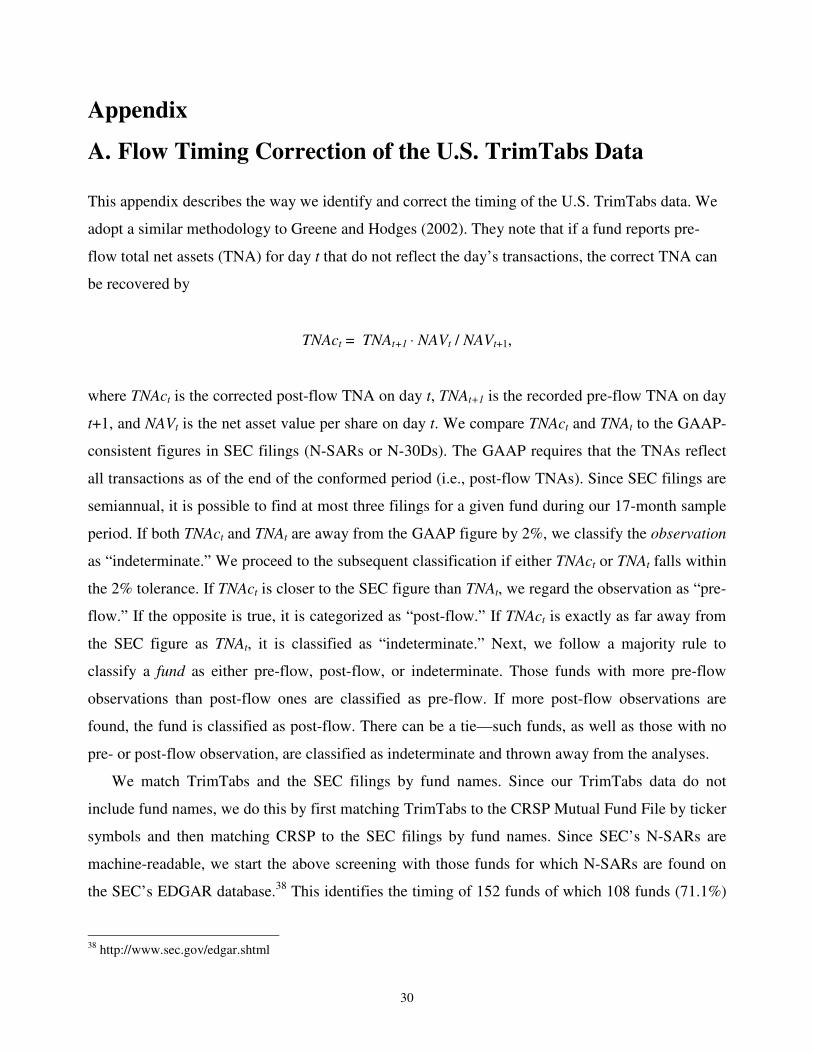
30

Appendix

A. Flow Timing Correction of the U.S. TrimTabs Data

This appendix describes the way we identify and correct the timing of the U.S. TrimTabs data. We

adopt a similar methodology to Greene and Hodges (2002). They note that if a fund reports pre-

flow total net assets (TNA) for day t that do not reflect the day’s transactions, the correct TNA can

be recovered by

TNAct = TNAt+1 ⋅ NAVt / NAVt+1,

where TNAct is the corrected post-flow TNA on day t, TNAt+1 is the recorded pre-flow TNA on day

t+1, and NAVt is the net asset value per share on day t. We compare TNAct and TNAt to the GAAP-

consistent figures in SEC filings (N-SARs or N-30Ds). The GAAP requires that the TNAs reflect

all transactions as of the end of the conformed period (i.e., post-flow TNAs). Since SEC filings are

semiannual, it is possible to find at most three filings for a given fund during our 17-month sample

period. If both TNAct and TNAt are away from the GAAP figure by 2%, we classify the observation

as “indeterminate.” We proceed to the subsequent classification if either TNAct or TNAt falls within

the 2% tolerance. If TNAct is closer to the SEC figure than TNAt, we regard the observation as “pre-

flow.” If the opposite is true, it is categorized as “post-flow.” If TNAct is exactly as far away from

the SEC figure as TNAt, it is classified as “indeterminate.” Next, we follow a majority rule to

classify a fund as either pre-flow, post-flow, or indeterminate. Those funds with more pre-flow

observations than post-flow ones are classified as pre-flow. If more post-flow observations are

found, the fund is classified as post-flow. There can be a tie—such funds, as well as those with no

pre- or post-flow observation, are classified as indeterminate and thrown away from the analyses.

We match TrimTabs and the SEC filings by fund names. Since our TrimTabs data do not

include fund names, we do this by first matching TrimTabs to the CRSP Mutual Fund File by ticker

symbols and then matching CRSP to the SEC filings by fund names. Since SEC’s N-SARs are

machine-readable, we start the above screening with those funds for which N-SARs are found on

the SEC’s EDGAR database.38 This identifies the timing of 152 funds of which 108 funds (71.1%)

38 http://www.sec.gov/edgar.shtml

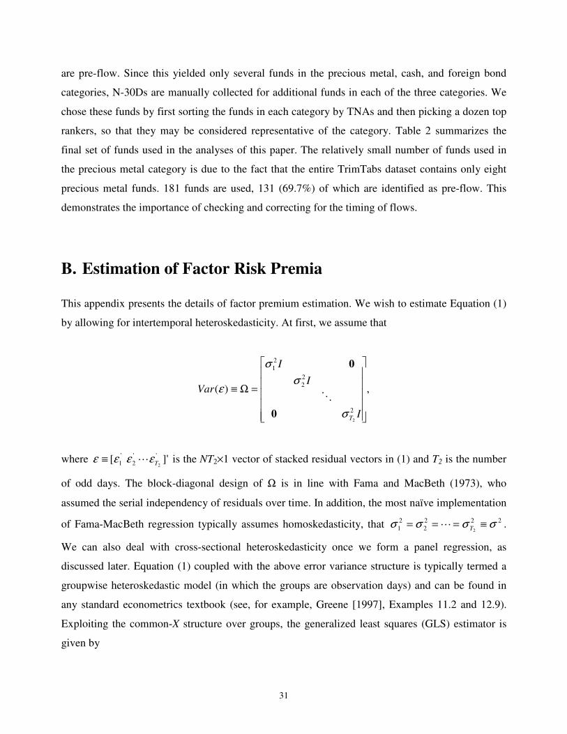
31

are pre-flow. Since this yielded only several funds in the precious metal, cash, and foreign bond

categories, N-30Ds are manually collected for additional funds in each of the three categories. We

chose these funds by first sorting the funds in each category by TNAs and then picking a dozen top

rankers, so that they may be considered representative of the category. Table 2 summarizes the

final set of funds used in the analyses of this paper. The relatively small number of funds used in

the precious metal category is due to the fact that the entire TrimTabs dataset contains only eight

precious metal funds. 181 funds are used, 131 (69.7%) of which are identified as pre-flow. This

demonstrates the importance of checking and correcting for the timing of flows.

B. Estimation of Factor Risk Premia

This appendix presents the details of factor premium estimation. We wish to estimate Equation (1)

by allowing for intertemporal heteroskedasticity. At first, we assume that

,)(

2

2

2

2

1

2

=Ω≡

I

I

I

Var

Tσ

σ

σ

ε

0

0

⋱

where ]'[ ''

2

'

1 2Tεεεε ⋯≡ is the NT2×1 vector of stacked residual vectors in (1) and T2 is the number

of odd days. The block-diagonal design of Ω is in line with Fama and MacBeth (1973), who

assumed the serial independency of residuals over time. In addition, the most naïve implementation

of Fama-MacBeth regression typically assumes homoskedasticity, that 222

2

2

1 2σσσσ ≡=== T⋯ .

We can also deal with cross-sectional heteroskedasticity once we form a panel regression, as

discussed later. Equation (1) coupled with the above error variance structure is typically termed a

groupwise heteroskedastic model (in which the groups are observation days) and can be found in

any standard econometrics textbook (see, for example, Greene [1997], Examples 11.2 and 12.9).

Exploiting the common-X structure over groups, the generalized least squares (GLS) estimator is

given by

32

,

'1

'1ˆ

,2

1

2

∑

∑∑

=

= •

−

t

tt

t

t

tt t

bw

RXXXσσ

λ

where ∑

≡

t

t

t

tw2

2

/1

/1

σ

σ and bt ≡ (X’X)-1

X’R•,t is the ordinary least squares (OLS) estimator for day

(group) t. Thus, the GLS estimator in this model is simply the weighted average of OLS estimators

over days. Following the common practice, we implement this as a two-step feasible GLS. In the

first step, the OLS is used to obtain a consistent estimate of Ω. That is, set 22 σσ ≡t or wt = 1/T2 to

obtain the OLS estimator .1

2

∑=t

tbT

λ The OLS residuals, λε XR tt −= •,ˆ , are used to estimate

Nttt /ˆˆˆ '2 εεσ = for every t. In the second step, the estimates of residual variances are fed back into

the above equation for λ . It can be shown that this is equivalent with a panel regression. t-statistics

for estimates of factor risk premia in Tables 11-13 are based on White’s (1980) heteroskedasticity-

consistent standard errors from the panel regression and are corrected also for cross-sectional

heteroskedasticity in this sense.

33

References Barber, Brad, 1999, “Noise Trader Risk, Odd-Lot Trading, and Security Returns,” Working Paper,

University of California at Davis. Barberis, Nicholas and Andrei Shleifer, 2003, “Style Investing,” Journal of Financial Economics,

68 (2), 161-199. Brennan, Michael J. and H. Henry Cao, 1996, “Information, Trade, and Derivative Securities,”

Review of Financial Studies, 9 (1), 163-208. Brennan, Michael J. and H. Henry Cao, 1997, “International Portfolio Investment Flows,” Journal

of Finance, 52 (5), 1851-1880. Brown, Stephen J. and William N. Goetzmann, 1997, “Mutual Fund Styles,” Journal of Financial

Economics, 43, 373-399. Brown, Stephen J., William N. Goetzmann, Takato Hiraki, Toshiyuki Otsuki, and Noriyoshi

Shiraishi, 2001, “The Japanese Open-End Fund Puzzle,” Journal of Business, 74 (1), 59-77. Carhart, Mark M., 1997, “On persistence in mutual fund performance,” Journal of Finance, 52 (1),

57-82. Chui, Andy, Sheridan Titman, and K. C. John Wei, 2000, “Momentum, Ownership Structure, and

Financial Crises: An Analysis of Asian Stock Markets,” Working paper, University of Texas at Austin.

De Long, J. Bradford and Andrei Shleifer, 1992, “Closed-end Fund Discounts,” Journal of

Portfolio Management, 18 (2), 46-53. De Long, J. Bradford, Andrei Shleifer, Lawrence H. Summers, and Robert J. Waldmann, 1990,

“Noise Trader Risk in Financial Markets,” Journal of Political Economy, 98 (4), 703-738. Edelen, Roger M. and Jerold B. Warner, 2001, “Aggregate Price Effects of Institutional Trading: A

Study of Mutual Fund Flow and Market Returns,” Journal of Financial Economics, 59, 195-220.

Elton, Edwin J., Martin J. Gruber, and Jeffrey A. Busse, 1998, “Do Investors Care about

Sentiment?,” Journal of Business, 71 (4), 477-500. Fama, Eugene F. and Kenneth R. French, 1993, “Common Risk Factors in The Returns on Bonds

and Stocks,” Journal of Financial Economics, 33, 3-56.

34

Fama, Eugene F. and James D. MacBeth, 1973, “Risk, Return, and Equilibrium: Empirical Tests,” Journal of Political Economy, 81 (3), 607-636.

Froot, Kenneth A. and Emil M. Dabora, 1999, “How Are Stock Prices Affected by the Location of

Trade?” Journal of Financial Economics, 53, 189-216. Froot, Kenneth A., Paul G. J. O’Connell, and Mark S. Seasholes, 2001, “The Portfolio Flows of

International Investors,” Journal of Financial Economics, 59, 151-193. Goetzmann, William N. and Massimo Massa, 2000a, “Index Funds and Stock Market Growth,”

forthcoming, The Journal of Business. Goetzmann, William N. and Massimo Massa, 2000b, “Daily Momentum and Contrarian Behavior

of Index Fund Investors” forthcoming, Journal of Financial and Quantitative Analysis. Goetzmann, William N., Massimo Massa, and K. Geert Rouwenhorst, 1999, “Behavioral Factors in

Mutual Fund Flows,” Working Paper, Yale School of Management. Greene, William H., 1997, Econometric Analysis, 3rd ed., Prentice Hall; New Jersey. Greene, Jason T. and Charles W. Hodges, 2002, “The Dilution Impact of Daily Fund Flows on

Open-end Mutual Funds,” Journal of Financial Economics, 65 (1), 131-158. Grinblatt, Mark and Matti Keloharju, 2000, “The Investment Behavior and Performance of Various

Investor Types: A Study of Finland’s Unique Data Set,” Journal of Financial Economics, 55 (1), 43-67.

Hamao, Yasushi, Ronald W. Masulis and Victor Ng, 1990, “Correlations in Price Changes and

Volatility across International Stock Markets,” Review of Financial Studies, 3 (2), 281-307. Ibbotson Associates, 2001, Stock, Bonds, Bills, and Inflation 2001 Yearbook, Ibbotson Associates;

Chicago, Illinois. Iihara, Yoshio, Hideaki Kiyoshi Kato and Toshifumi Tokunaga, 2001, “Investors’ Herding on the

Tokyo Stock Exchange,” International Review of Finance, 2:1/2, 71-98. Jagannathan, Ravi and Zhenyu Wang, 1996, “The Conditional CAPM and the Cross-Section of

Expected Returns,” Journal of Finance, 51 (1), 3-53. Jagannathan, Ravi and Zhenyu Wang, 1998, “An Asymptotic Theory for Estimating Beta-Pricing

Models Using Cross-Sectional Regression,” Journal of Finance, 53 (4), 1285-1309. Jegadeesh, Narashimhan and Sheridan Titman, 1993, “Returns to Buying Winners and Selling

Losers: Implications for Stock Market Efficiency,” Journal of Finance, 48 (1), March, 65-91.

35

Jegadeesh, Narashimhan and Sheridan Titman, 2001, “Profitability of Momentum Strategies: An Evaluation of Alternative Explanations,” Journal of Finance, 56 (2), 699-720.

Jones, Christopher S., 2001, “Extracting Factors from Heteroskedastic Asset Returns,” Journal of

Financial Economics, 62, 293-325. Kamesaka, Akiko Murase, John R. Nofsinger, and Hidetaka Kawakita, 2003, “Investment Patterns

and Performance of Investor Groups in Japan,” Pacific Basin Finance Journal, 11(1), 1-22. Lee, Charles M. C., Andrei Shleifer, and Richard H. Thaler, 1991, “Investor Sentiment and The

Closed-End Fund Puzzle,” Journal of Finance, 46 (1), 75-109. Lin, Wen-Ling, Robert F. Engle, and Takatoshi Ito, 1994, “Do Bulls and Bears Move across

Borders? International Transmission of Stock Returns and Volatility,” Review of Financial

Studies, 7 (3), 507-538. Lin, Wen-Ling and Takatoshi Ito, 1994, “Price Volatility and Volume Spillovers between the

Tokyo and New York Stock Markets,” in Frankel, Jeffrey A., ed., The Internationalization

of Equity Markets, 309-343. Roll, Richard and Stephen A. Ross, 1980, “An Empirical Investigation of the Arbitrage Pricing

Theory,” Journal of Finance, 35 (5), 1073-1103. Rouwenhorst, K. Geert, 1998, “International Momentum Strategies,” Journal of Finance, 53 (1),

267-284. Shiller, Robert J., 1999, “Measuring Bubble Expectations and Investor Confidence,” Cowles

Foundation Discussion Paper, #1212, Yale University. Shiller, Robert J., Fumiko Kon-Ya and Yoshiro Tsutsui, 1996, “Why Did the Nikkei Crash?

Expanding the Scope of Expectations Data Collection,” Review of Economics and Statistics, 78 (1), 156-64.

Warther, Vincent A., 1995, “Aggregate Mutual Fund Flows and Security Returns,” Journal of

Financial Economics, 39, 209-235. Warther, Vincent A., 1998, “Has the Rise of Mutual Funds Increased Market Instability?”

Brookings-Wharton Papers on Financial Services, 239-62. White, Halbert, 1980, “A Heteroskedasticity-Consistent Covariance Matrix Estimator and a Direct

Test for Heteroskedasticity,” Econometrica, 48 (4), 817-38. Zitzewitz, Eric, 2003, “Who Cares about Shareholders? Arbitrage-Proofing Mutual Funds,”

Journal of Law, Economics and Organization, 19 (2), 245-280.

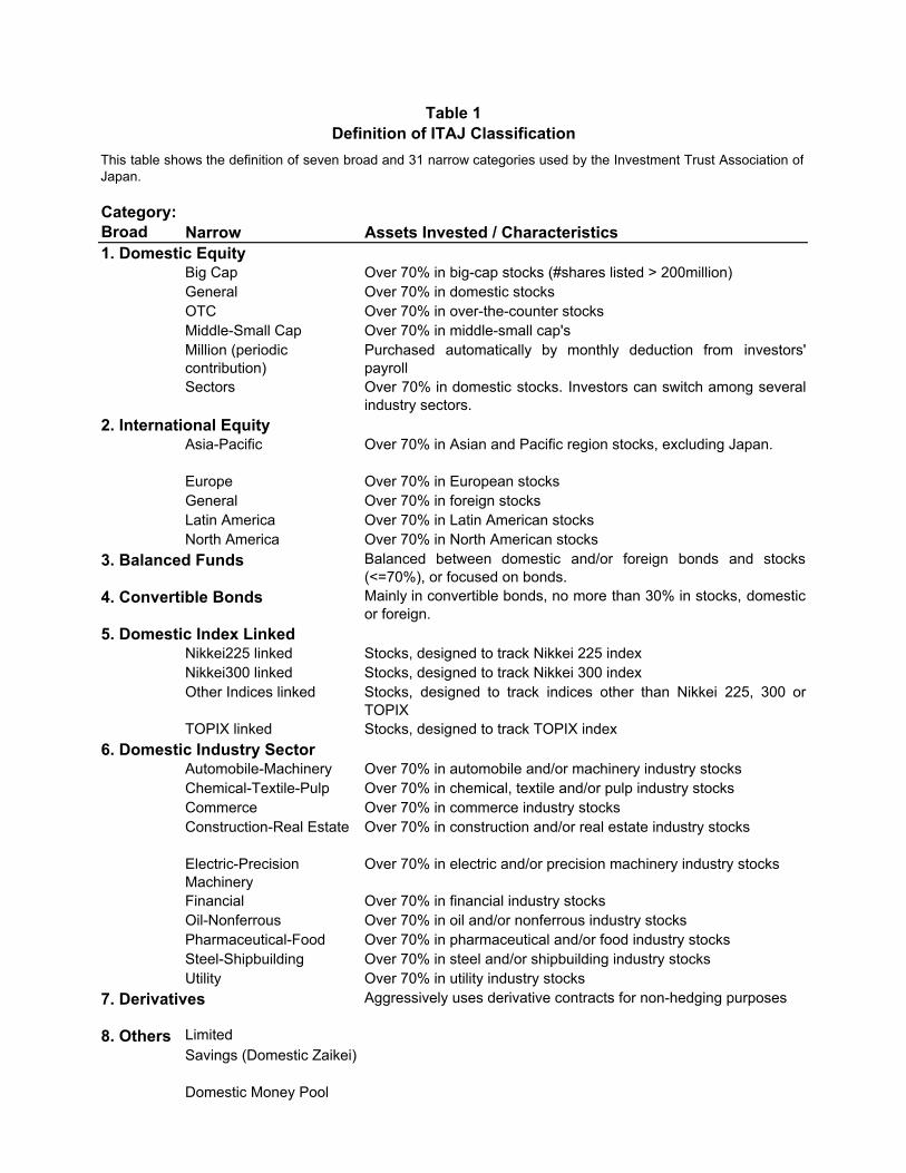
Table 1Definition of ITAJ Classification

Category:Broad Narrow Assets Invested / Characteristics1. Domestic Equity

Big Cap Over 70% in big-cap stocks (#shares listed > 200million)General Over 70% in domestic stocksOTC Over 70% in over-the-counter stocksMiddle-Small Cap Over 70% in middle-small cap'sMillion (periodic contribution)

Purchased automatically by monthly deduction from investors'payroll

Sectors Over 70% in domestic stocks. Investors can switch among severalindustry sectors.

2. International EquityAsia-Pacific Over 70% in Asian and Pacific region stocks, excluding Japan.

Europe Over 70% in European stocksGeneral Over 70% in foreign stocksLatin America Over 70% in Latin American stocksNorth America Over 70% in North American stocks

3. Balanced Funds Balanced between domestic and/or foreign bonds and stocks(<=70%), or focused on bonds.

4. Convertible Bonds Mainly in convertible bonds, no more than 30% in stocks, domesticor foreign.

5. Domestic Index LinkedNikkei225 linked Stocks, designed to track Nikkei 225 indexNikkei300 linked Stocks, designed to track Nikkei 300 indexOther Indices linked Stocks, designed to track indices other than Nikkei 225, 300 or

TOPIXTOPIX linked Stocks, designed to track TOPIX index

6. Domestic Industry SectorAutomobile-Machinery Over 70% in automobile and/or machinery industry stocksChemical-Textile-Pulp Over 70% in chemical, textile and/or pulp industry stocksCommerce Over 70% in commerce industry stocksConstruction-Real Estate Over 70% in construction and/or real estate industry stocks

Electric-Precision Machinery

Over 70% in electric and/or precision machinery industry stocks

Financial Over 70% in financial industry stocksOil-Nonferrous Over 70% in oil and/or nonferrous industry stocksPharmaceutical-Food Over 70% in pharmaceutical and/or food industry stocksSteel-Shipbuilding Over 70% in steel and/or shipbuilding industry stocksUtility Over 70% in utility industry stocks

7. Derivatives Aggressively uses derivative contracts for non-hedging purposes

8. Others LimitedSavings (Domestic Zaikei)

Domestic Money Pool

This table shows the definition of seven broad and 31 narrow categories used by the Investment Trust Association ofJapan.

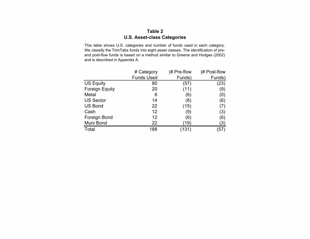
Table 2U.S. Asset-class Categories

# Category Funds Used

(# Pre-flow Funds)

(# Post-flow Funds)

US Equity 80 (57) (23)Foreign Equity 20 (11) (9)Metal 6 (6) (0)US Sector 14 (8) (6)US Bond 22 (15) (7)Cash 12 (9) (3)Foreign Bond 12 (6) (6)Muni Bond 22 (19) (3)Total 188 (131) (57)

This table shows U.S. categories and number of funds used in each category.We classify the TrimTabs funds into eight asset classes. The identification of pre-and post-flow funds is based on a method similar to Greene and Hodges (2002)and is described in Appendix A.

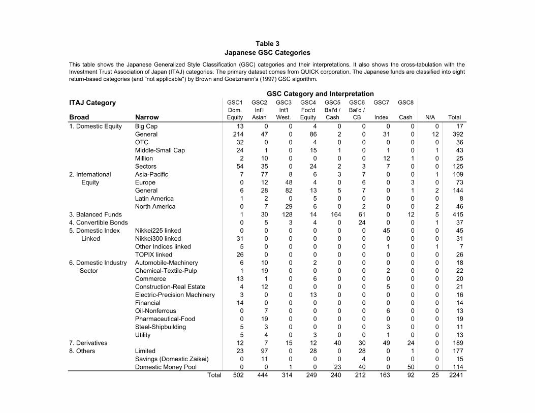
Table 3Japanese GSC Categories

GSC Category and InterpretationITAJ Category GSC1 GSC2 GSC3 GSC4 GSC5 GSC6 GSC7 GSC8

Broad NarrowDom. Equity

Int'l Asian

Int'l West.

Foc'd Equity

Bal'd / Cash

Bal'd / CB Index Cash N/A Total

1. Domestic Equity Big Cap 13 0 0 4 0 0 0 0 0 17General 214 47 0 86 2 0 31 0 12 392OTC 32 0 0 4 0 0 0 0 0 36Middle-Small Cap 24 1 0 15 1 0 1 0 1 43Million 2 10 0 0 0 0 12 1 0 25Sectors 54 35 0 24 2 3 7 0 0 125

2. International Asia-Pacific 7 77 8 6 3 7 0 0 1 109 Equity Europe 0 12 48 4 0 6 0 3 0 73

General 6 28 82 13 5 7 0 1 2 144Latin America 1 2 0 5 0 0 0 0 0 8North America 0 7 29 6 0 2 0 0 2 46

3. Balanced Funds 1 30 128 14 164 61 0 12 5 4154. Convertible Bonds 0 5 3 4 0 24 0 0 1 375. Domestic Index Nikkei225 linked 0 0 0 0 0 0 45 0 0 45 Linked Nikkei300 linked 31 0 0 0 0 0 0 0 0 31

Other Indices linked 5 0 0 0 0 0 1 0 1 7TOPIX linked 26 0 0 0 0 0 0 0 0 26

6. Domestic Industry Automobile-Machinery 6 10 0 2 0 0 0 0 0 18 Sector Chemical-Textile-Pulp 1 19 0 0 0 0 2 0 0 22

Commerce 13 1 0 6 0 0 0 0 0 20Construction-Real Estate 4 12 0 0 0 0 5 0 0 21Electric-Precision Machinery 3 0 0 13 0 0 0 0 0 16Financial 14 0 0 0 0 0 0 0 0 14Oil-Nonferrous 0 7 0 0 0 0 6 0 0 13Pharmaceutical-Food 0 19 0 0 0 0 0 0 0 19Steel-Shipbuilding 5 3 0 0 0 0 3 0 0 11Utility 5 4 0 3 0 0 1 0 0 13

7. Derivatives 12 7 15 12 40 30 49 24 0 1898. Others Limited 23 97 0 28 0 28 0 1 0 177

Savings (Domestic Zaikei) 0 11 0 0 0 4 0 0 0 15Domestic Money Pool 0 0 1 0 23 40 0 50 0 114

Total 502 444 314 249 240 212 163 92 25 2241

This table shows the Japanese Generalized Style Classification (GSC) categories and their interpretations. It also shows the cross-tabulation with theInvestment Trust Association of Japan (ITAJ) categories. The primary dataset comes from QUICK corporation. The Japanese funds are classified into eightreturn-based categories (and "not applicable") by Brown and Goetzmann's (1997) GSC algorithm.

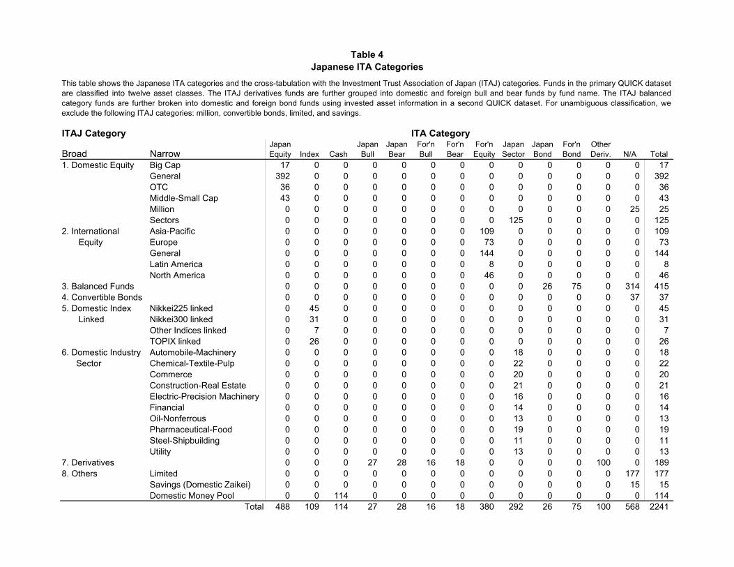
Table 4Japanese ITA Categories

ITAJ Category ITA Category

Broad NarrowJapan Equity Index Cash

Japan Bull

Japan Bear

For'n Bull

For'n Bear

For'n Equity

Japan Sector

Japan Bond

For'n Bond

Other Deriv. N/A Total

1. Domestic Equity Big Cap 17 0 0 0 0 0 0 0 0 0 0 0 0 17General 392 0 0 0 0 0 0 0 0 0 0 0 0 392OTC 36 0 0 0 0 0 0 0 0 0 0 0 0 36Middle-Small Cap 43 0 0 0 0 0 0 0 0 0 0 0 0 43Million 0 0 0 0 0 0 0 0 0 0 0 0 25 25Sectors 0 0 0 0 0 0 0 0 125 0 0 0 0 125

2. International Asia-Pacific 0 0 0 0 0 0 0 109 0 0 0 0 0 109 Equity Europe 0 0 0 0 0 0 0 73 0 0 0 0 0 73

General 0 0 0 0 0 0 0 144 0 0 0 0 0 144Latin America 0 0 0 0 0 0 0 8 0 0 0 0 0 8North America 0 0 0 0 0 0 0 46 0 0 0 0 0 46

3. Balanced Funds 0 0 0 0 0 0 0 0 0 26 75 0 314 4154. Convertible Bonds 0 0 0 0 0 0 0 0 0 0 0 0 37 375. Domestic Index Nikkei225 linked 0 45 0 0 0 0 0 0 0 0 0 0 0 45 Linked Nikkei300 linked 0 31 0 0 0 0 0 0 0 0 0 0 0 31

Other Indices linked 0 7 0 0 0 0 0 0 0 0 0 0 0 7TOPIX linked 0 26 0 0 0 0 0 0 0 0 0 0 0 26

6. Domestic Industry Automobile-Machinery 0 0 0 0 0 0 0 0 18 0 0 0 0 18 Sector Chemical-Textile-Pulp 0 0 0 0 0 0 0 0 22 0 0 0 0 22

Commerce 0 0 0 0 0 0 0 0 20 0 0 0 0 20Construction-Real Estate 0 0 0 0 0 0 0 0 21 0 0 0 0 21Electric-Precision Machinery 0 0 0 0 0 0 0 0 16 0 0 0 0 16Financial 0 0 0 0 0 0 0 0 14 0 0 0 0 14Oil-Nonferrous 0 0 0 0 0 0 0 0 13 0 0 0 0 13Pharmaceutical-Food 0 0 0 0 0 0 0 0 19 0 0 0 0 19Steel-Shipbuilding 0 0 0 0 0 0 0 0 11 0 0 0 0 11Utility 0 0 0 0 0 0 0 0 13 0 0 0 0 13

7. Derivatives 0 0 0 27 28 16 18 0 0 0 0 100 0 1898. Others Limited 0 0 0 0 0 0 0 0 0 0 0 0 177 177

Savings (Domestic Zaikei) 0 0 0 0 0 0 0 0 0 0 0 0 15 15Domestic Money Pool 0 0 114 0 0 0 0 0 0 0 0 0 0 114

Total 488 109 114 27 28 16 18 380 292 26 75 100 568 2241

This table shows the Japanese ITA categories and the cross-tabulation with the Investment Trust Association of Japan (ITAJ) categories. Funds in the primary QUICK datasetare classified into twelve asset classes. The ITAJ derivatives funds are further grouped into domestic and foreign bull and bear funds by fund name. The ITAJ balancedcategory funds are further broken into domestic and foreign bond funds using invested asset information in a second QUICK dataset. For unambiguous classification, weexclude the following ITAJ categories: million, convertible bonds, limited, and savings.

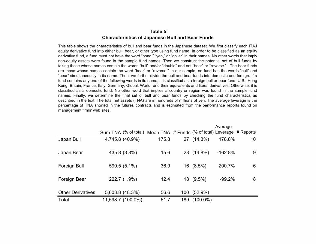
Table 5Characteristics of Japanese Bull and Bear Funds

Sum TNA (% of total) Mean TNA # Funds (% of total)Average Leverage # Reports

Japan Bull 4,745.8 (40.9%) 175.8 27 (14.3%) 178.8% 10

Japan Bear 435.8 (3.8%) 15.6 28 (14.8%) -162.8% 9

Foreign Bull 590.5 (5.1%) 36.9 16 (8.5%) 200.7% 6

Foreign Bear 222.7 (1.9%) 12.4 18 (9.5%) -99.2% 8

Other Derivatives 5,603.8 (48.3%) 56.6 100 (52.9%)Total 11,598.7 (100.0%) 61.7 189 (100.0%)

This table shows the characteristics of bull and bear funds in the Japanese dataset. We first classify each ITAJequity derivative fund into either bull, bear, or other type using fund name. In order to be classified as an equityderivative fund, a fund must not have the word “bond,” “yen,” or “dollar” in their names. No other words that implynon-equity assets were found in the sample fund names. Then we construct the potential set of bull funds bytaking those whose names contain the words “bull” and/or “double” and not “bear” or “reverse.” The bear fundsare those whose names contain the word ”bear” or “reverse.” In our sample, no fund has the words “bull” and“bear” simultaneously in its name. Then, we further divide the bull and bear funds into domestic and foreign. If afund contains any one of the following words in its name, it is classified as a foreign bull or bear fund: U.S., HongKong, Britain, France, Italy, Germany, Global, World, and their equivalents and literal derivatives. Otherwise, it isclassified as a domestic fund. No other word that implies a country or region was found in the sample fundnames. Finally, we determine the final set of bull and bear funds by checking the fund characteristics asdescribed in the text. The total net assets (TNA) are in hundreds of millions of yen. The average leverage is thepercentage of TNA shorted in the futures contracts and is estimated from the performance reports found onmanagement firms' web sites.

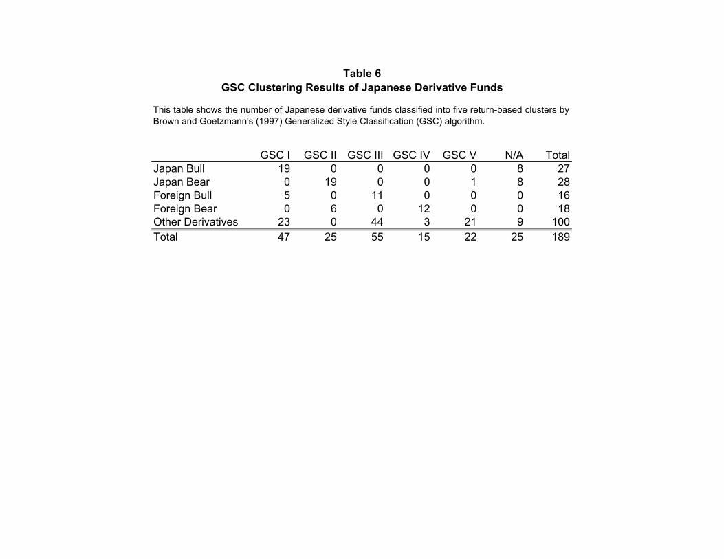
Table 6GSC Clustering Results of Japanese Derivative Funds

GSC I GSC II GSC III GSC IV GSC V N/A TotalJapan Bull 19 0 0 0 0 8 27Japan Bear 0 19 0 0 1 8 28Foreign Bull 5 0 11 0 0 0 16Foreign Bear 0 6 0 12 0 0 18Other Derivatives 23 0 44 3 21 9 100Total 47 25 55 15 22 25 189

This table shows the number of Japanese derivative funds classified into five return-based clusters byBrown and Goetzmann's (1997) Generalized Style Classification (GSC) algorithm.

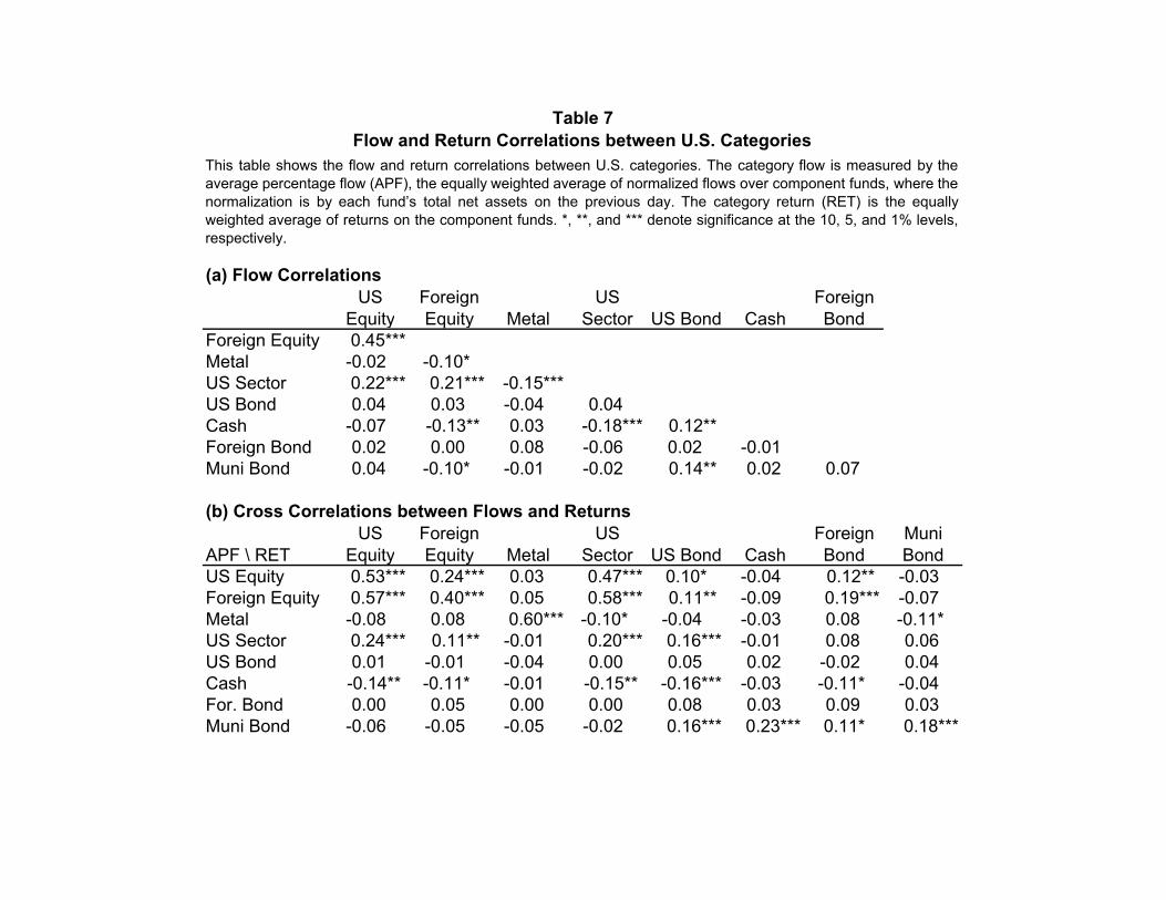
Table 7Flow and Return Correlations between U.S. Categories

(a) Flow CorrelationsUS

EquityForeign Equity Metal

US Sector US Bond Cash

Foreign Bond

Foreign Equity 0.45***Metal -0.02 -0.10* US Sector 0.22*** 0.21*** -0.15***US Bond 0.04 0.03 -0.04 0.04 Cash -0.07 -0.13** 0.03 -0.18*** 0.12** Foreign Bond 0.02 0.00 0.08 -0.06 0.02 -0.01 Muni Bond 0.04 -0.10* -0.01 -0.02 0.14** 0.02 0.07

(b) Cross Correlations between Flows and Returns

APF \ RETUS

EquityForeign Equity Metal

US Sector US Bond Cash

Foreign Bond

Muni Bond

US Equity 0.53*** 0.24*** 0.03 0.47*** 0.10* -0.04 0.12** -0.03 Foreign Equity 0.57*** 0.40*** 0.05 0.58*** 0.11** -0.09 0.19*** -0.07 Metal -0.08 0.08 0.60*** -0.10* -0.04 -0.03 0.08 -0.11* US Sector 0.24*** 0.11** -0.01 0.20*** 0.16*** -0.01 0.08 0.06 US Bond 0.01 -0.01 -0.04 0.00 0.05 0.02 -0.02 0.04 Cash -0.14** -0.11* -0.01 -0.15** -0.16*** -0.03 -0.11* -0.04 For. Bond 0.00 0.05 0.00 0.00 0.08 0.03 0.09 0.03 Muni Bond -0.06 -0.05 -0.05 -0.02 0.16*** 0.23*** 0.11* 0.18***

This table shows the flow and return correlations between U.S. categories. The category flow is measured by theaverage percentage flow (APF), the equally weighted average of normalized flows over component funds, where thenormalization is by each fund’s total net assets on the previous day. The category return (RET) is the equallyweighted average of returns on the component funds. *, **, and *** denote significance at the 10, 5, and 1% levels,respectively.

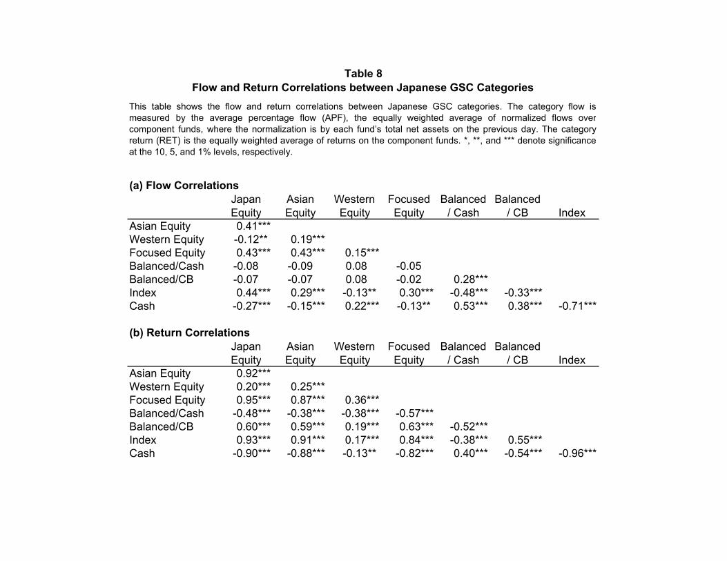
Table 8Flow and Return Correlations between Japanese GSC Categories

(a) Flow CorrelationsJapan Equity

Asian Equity

Western Equity

Focused Equity

Balanced / Cash

Balanced / CB Index

Asian Equity 0.41***Western Equity -0.12** 0.19***Focused Equity 0.43*** 0.43*** 0.15***Balanced/Cash -0.08 -0.09 0.08 -0.05 Balanced/CB -0.07 -0.07 0.08 -0.02 0.28***Index 0.44*** 0.29*** -0.13** 0.30*** -0.48*** -0.33***Cash -0.27*** -0.15*** 0.22*** -0.13** 0.53*** 0.38*** -0.71***

(b) Return CorrelationsJapan Equity

Asian Equity

Western Equity

Focused Equity

Balanced / Cash

Balanced / CB Index

Asian Equity 0.92***Western Equity 0.20*** 0.25***Focused Equity 0.95*** 0.87*** 0.36***Balanced/Cash -0.48*** -0.38*** -0.38*** -0.57***Balanced/CB 0.60*** 0.59*** 0.19*** 0.63*** -0.52***Index 0.93*** 0.91*** 0.17*** 0.84*** -0.38*** 0.55***Cash -0.90*** -0.88*** -0.13** -0.82*** 0.40*** -0.54*** -0.96***

This table shows the flow and return correlations between Japanese GSC categories. The category flow ismeasured by the average percentage flow (APF), the equally weighted average of normalized flows overcomponent funds, where the normalization is by each fund’s total net assets on the previous day. The categoryreturn (RET) is the equally weighted average of returns on the component funds. *, **, and *** denote significanceat the 10, 5, and 1% levels, respectively.

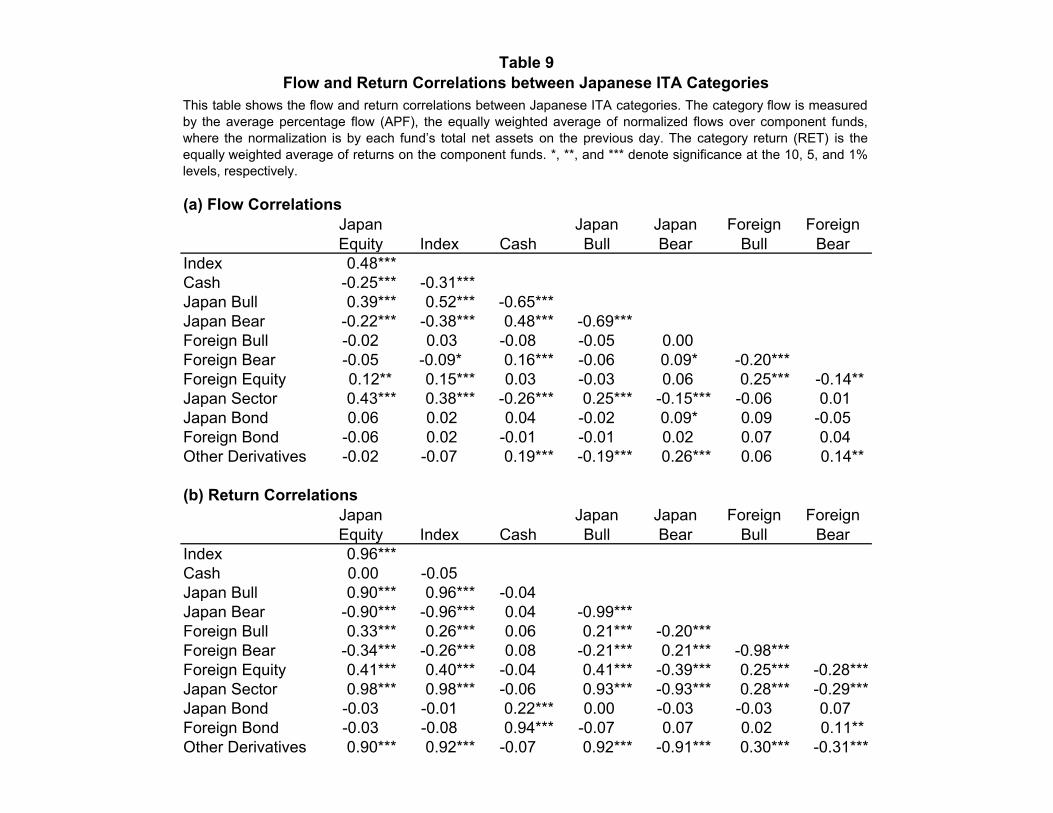
Table 9Flow and Return Correlations between Japanese ITA Categories

(a) Flow CorrelationsJapan Equity Index Cash

Japan Bull

Japan Bear

Foreign Bull

Foreign Bear

Index 0.48***Cash -0.25*** -0.31***Japan Bull 0.39*** 0.52*** -0.65***Japan Bear -0.22*** -0.38*** 0.48*** -0.69***Foreign Bull -0.02 0.03 -0.08 -0.05 0.00 Foreign Bear -0.05 -0.09* 0.16*** -0.06 0.09* -0.20***Foreign Equity 0.12** 0.15*** 0.03 -0.03 0.06 0.25*** -0.14** Japan Sector 0.43*** 0.38*** -0.26*** 0.25*** -0.15*** -0.06 0.01 Japan Bond 0.06 0.02 0.04 -0.02 0.09* 0.09 -0.05 Foreign Bond -0.06 0.02 -0.01 -0.01 0.02 0.07 0.04 Other Derivatives -0.02 -0.07 0.19*** -0.19*** 0.26*** 0.06 0.14**

(b) Return CorrelationsJapan Equity Index Cash

Japan Bull

Japan Bear

Foreign Bull

Foreign Bear

Index 0.96***Cash 0.00 -0.05 Japan Bull 0.90*** 0.96*** -0.04 Japan Bear -0.90*** -0.96*** 0.04 -0.99***Foreign Bull 0.33*** 0.26*** 0.06 0.21*** -0.20***Foreign Bear -0.34*** -0.26*** 0.08 -0.21*** 0.21*** -0.98***Foreign Equity 0.41*** 0.40*** -0.04 0.41*** -0.39*** 0.25*** -0.28***Japan Sector 0.98*** 0.98*** -0.06 0.93*** -0.93*** 0.28*** -0.29***Japan Bond -0.03 -0.01 0.22*** 0.00 -0.03 -0.03 0.07 Foreign Bond -0.03 -0.08 0.94*** -0.07 0.07 0.02 0.11** Other Derivatives 0.90*** 0.92*** -0.07 0.92*** -0.91*** 0.30*** -0.31***

This table shows the flow and return correlations between Japanese ITA categories. The category flow is measuredby the average percentage flow (APF), the equally weighted average of normalized flows over component funds,where the normalization is by each fund’s total net assets on the previous day. The category return (RET) is theequally weighted average of returns on the component funds. *, **, and *** denote significance at the 10, 5, and 1%levels, respectively.

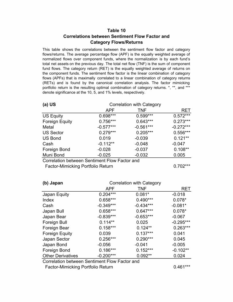
Table 10Correlations between Sentiment Flow Factor and

Category Flows/Returns

(a) US Correlation with CategoryAPF TNF RET

US Equity 0.698*** 0.599*** 0.572***Foreign Equity 0.756*** 0.643*** 0.273***Metal -0.577*** -0.561*** -0.272***US Sector 0.279*** 0.205*** 0.556***US Bond 0.019 -0.039 0.121** Cash -0.112** -0.048 -0.047 Foreign Bond -0.028 -0.037 0.108** Muni Bond -0.025 -0.032 0.005 Correlation between Sentiment Flow Factor and Factor-Mimicking Portfolio Return 0.702***

(b) Japan Correlation with CategoryAPF TNF RET

Japan Equity 0.204*** 0.081* -0.018 Index 0.658*** 0.490*** 0.078* Cash -0.349*** -0.434*** -0.081* Japan Bull 0.658*** 0.647*** 0.078* Japan Bear -0.839*** -0.653*** -0.067 Foreign Bull 0.114** 0.025 -0.295***Foreign Bear 0.158*** 0.124** 0.263***Foreign Equity 0.039 0.137*** 0.041 Japan Sector 0.256*** 0.290*** 0.045 Japan Bond -0.056 -0.041 -0.005 Foreign Bond 0.186*** 0.152*** -0.102** Other Derivatives -0.200*** 0.092** 0.024 Correlation between Sentiment Flow Factor and Factor-Mimicking Portfolio Return 0.461***

This table shows the correlations between the sentiment flow factor and categoryflows/returns. The average percentage flow (APF) is the equally weighted average ofnormalized flows over component funds, where the normalization is by each fund’stotal net assets on the previous day. The total net flow (TNF) is the sum of componentfund flows. The category return (RET) is the equally weighted average of returns onthe component funds. The sentiment flow factor is the linear combination of categoryflows (APFs) that is maximally correlated to a linear combination of category returns(RETs) and is found by the canonical correlation analysis. The factor mimickingportfolio return is the resulting optimal combination of category returns. *, **, and ***denote significance at the 10, 5, and 1% levels, respectively.

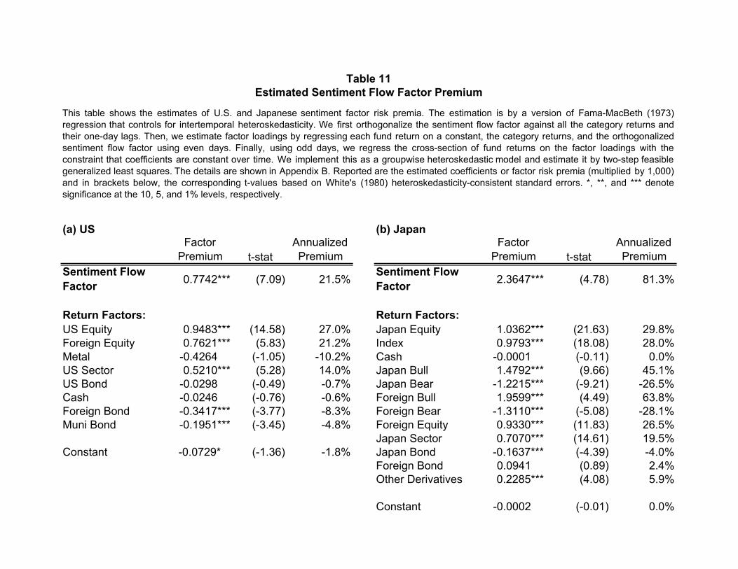
Table 11Estimated Sentiment Flow Factor Premium

(a) US (b) JapanFactor

Premium t-statAnnualized Premium

Factor Premium t-stat

Annualized Premium

Sentiment Flow Factor 0.7742*** (7.09) 21.5% Sentiment Flow

Factor 2.3647*** (4.78) 81.3%

Return Factors: Return Factors:US Equity 0.9483*** (14.58) 27.0% Japan Equity 1.0362*** (21.63) 29.8%Foreign Equity 0.7621*** (5.83) 21.2% Index 0.9793*** (18.08) 28.0%Metal -0.4264 (-1.05) -10.2% Cash -0.0001 (-0.11) 0.0%US Sector 0.5210*** (5.28) 14.0% Japan Bull 1.4792*** (9.66) 45.1%US Bond -0.0298 (-0.49) -0.7% Japan Bear -1.2215*** (-9.21) -26.5%Cash -0.0246 (-0.76) -0.6% Foreign Bull 1.9599*** (4.49) 63.8%Foreign Bond -0.3417*** (-3.77) -8.3% Foreign Bear -1.3110*** (-5.08) -28.1%Muni Bond -0.1951*** (-3.45) -4.8% Foreign Equity 0.9330*** (11.83) 26.5%

Japan Sector 0.7070*** (14.61) 19.5%Constant -0.0729* (-1.36) -1.8% Japan Bond -0.1637*** (-4.39) -4.0%

Foreign Bond 0.0941 (0.89) 2.4%Other Derivatives 0.2285*** (4.08) 5.9%

Constant -0.0002 (-0.01) 0.0%

This table shows the estimates of U.S. and Japanese sentiment factor risk premia. The estimation is by a version of Fama-MacBeth (1973)regression that controls for intertemporal heteroskedasticity. We first orthogonalize the sentiment flow factor against all the category returns andtheir one-day lags. Then, we estimate factor loadings by regressing each fund return on a constant, the category returns, and the orthogonalizedsentiment flow factor using even days. Finally, using odd days, we regress the cross-section of fund returns on the factor loadings with theconstraint that coefficients are constant over time. We implement this as a groupwise heteroskedastic model and estimate it by two-step feasiblegeneralized least squares. The details are shown in Appendix B. Reported are the estimated coefficients or factor risk premia (multiplied by 1,000)and in brackets below, the corresponding t-values based on White's (1980) heteroskedasticity-consistent standard errors. *, **, and *** denotesignificance at the 10, 5, and 1% levels, respectively.

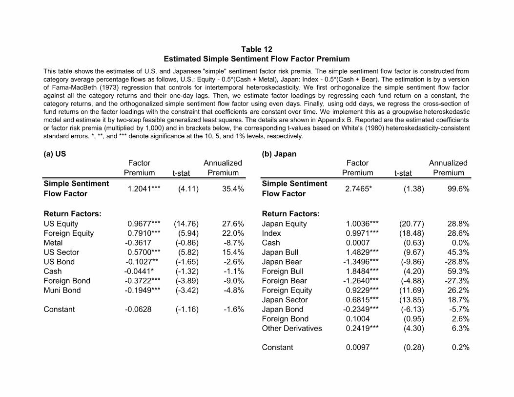
Table 12Estimated Simple Sentiment Flow Factor Premium

(a) US (b) JapanFactor

Premium t-statAnnualized Premium

Factor Premium t-stat

Annualized Premium

Simple Sentiment Flow Factor 1.2041*** (4.11) 35.4% Simple Sentiment

Flow Factor 2.7465* (1.38) 99.6%

Return Factors: Return Factors:US Equity 0.9677*** (14.76) 27.6% Japan Equity 1.0036*** (20.77) 28.8%Foreign Equity 0.7910*** (5.94) 22.0% Index 0.9971*** (18.48) 28.6%Metal -0.3617 (-0.86) -8.7% Cash 0.0007 (0.63) 0.0%US Sector 0.5700*** (5.82) 15.4% Japan Bull 1.4829*** (9.67) 45.3%US Bond -0.1027** (-1.65) -2.6% Japan Bear -1.3496*** (-9.86) -28.8%Cash -0.0441* (-1.32) -1.1% Foreign Bull 1.8484*** (4.20) 59.3%Foreign Bond -0.3722*** (-3.89) -9.0% Foreign Bear -1.2640*** (-4.88) -27.3%Muni Bond -0.1949*** (-3.42) -4.8% Foreign Equity 0.9229*** (11.69) 26.2%

Japan Sector 0.6815*** (13.85) 18.7%Constant -0.0628 (-1.16) -1.6% Japan Bond -0.2349*** (-6.13) -5.7%

Foreign Bond 0.1004 (0.95) 2.6%Other Derivatives 0.2419*** (4.30) 6.3%

Constant 0.0097 (0.28) 0.2%

This table shows the estimates of U.S. and Japanese "simple" sentiment factor risk premia. The simple sentiment flow factor is constructed fromcategory average percentage flows as follows, U.S.: Equity - 0.5*(Cash + Metal), Japan: Index - 0.5*(Cash + Bear). The estimation is by a versionof Fama-MacBeth (1973) regression that controls for intertemporal heteroskedasticity. We first orthogonalize the simple sentiment flow factoragainst all the category returns and their one-day lags. Then, we estimate factor loadings by regressing each fund return on a constant, thecategory returns, and the orthogonalized simple sentiment flow factor using even days. Finally, using odd days, we regress the cross-section offund returns on the factor loadings with the constraint that coefficients are constant over time. We implement this as a groupwise heteroskedasticmodel and estimate it by two-step feasible generalized least squares. The details are shown in Appendix B. Reported are the estimated coefficientsor factor risk premia (multiplied by 1,000) and in brackets below, the corresponding t-values based on White's (1980) heteroskedasticity-consistentstandard errors. *, **, and *** denote significance at the 10, 5, and 1% levels, respectively.

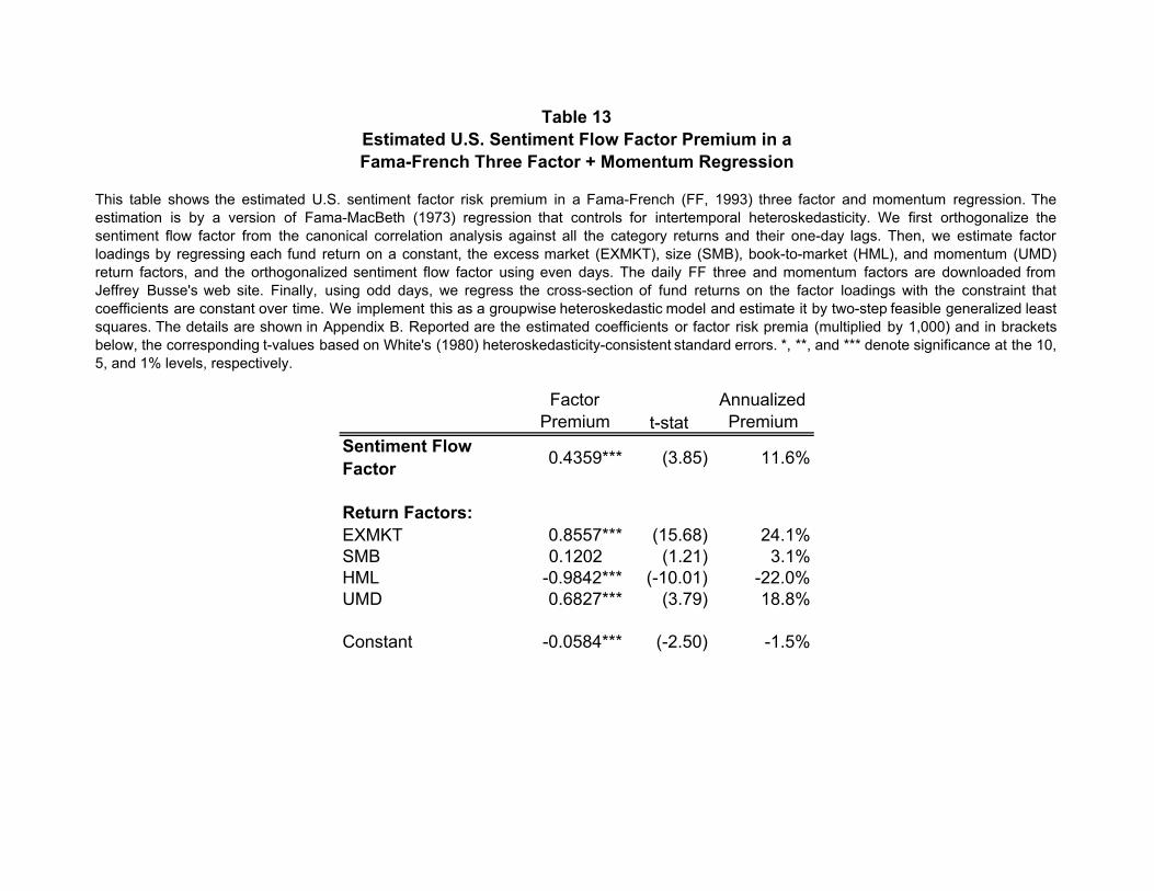
Table 13Estimated U.S. Sentiment Flow Factor Premium in aFama-French Three Factor + Momentum Regression

Factor Premium t-stat

Annualized Premium

Sentiment Flow Factor 0.4359*** (3.85) 11.6%

Return Factors:EXMKT 0.8557*** (15.68) 24.1%SMB 0.1202 (1.21) 3.1%HML -0.9842*** (-10.01) -22.0%UMD 0.6827*** (3.79) 18.8%

Constant -0.0584*** (-2.50) -1.5%

This table shows the estimated U.S. sentiment factor risk premium in a Fama-French (FF, 1993) three factor and momentum regression. Theestimation is by a version of Fama-MacBeth (1973) regression that controls for intertemporal heteroskedasticity. We first orthogonalize thesentiment flow factor from the canonical correlation analysis against all the category returns and their one-day lags. Then, we estimate factorloadings by regressing each fund return on a constant, the excess market (EXMKT), size (SMB), book-to-market (HML), and momentum (UMD)return factors, and the orthogonalized sentiment flow factor using even days. The daily FF three and momentum factors are downloaded fromJeffrey Busse's web site. Finally, using odd days, we regress the cross-section of fund returns on the factor loadings with the constraint thatcoefficients are constant over time. We implement this as a groupwise heteroskedastic model and estimate it by two-step feasible generalized leastsquares. The details are shown in Appendix B. Reported are the estimated coefficients or factor risk premia (multiplied by 1,000) and in bracketsbelow, the corresponding t-values based on White's (1980) heteroskedasticity-consistent standard errors. *, **, and *** denote significance at the 10,5, and 1% levels, respectively.

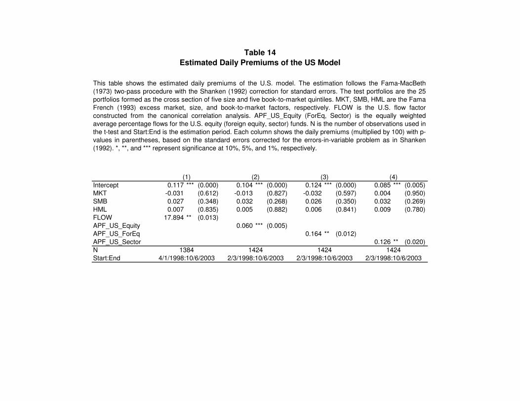
Table 14

Estimated Daily Premiums of the US Model

(1) (2) (3) (4)

Intercept 0.117 *** (0.000) 0.104 *** (0.000) 0.124 *** (0.000) 0.085 *** (0.005)

MKT -0.031 (0.612) -0.013 (0.827) -0.032 (0.597) 0.004 (0.950)

SMB 0.027 (0.348) 0.032 (0.268) 0.026 (0.350) 0.032 (0.269)

HML 0.007 (0.835) 0.005 (0.882) 0.006 (0.841) 0.009 (0.780)

FLOW 17.894 ** (0.013)

APF_US_Equity 0.060 *** (0.005)

APF_US_ForEq 0.164 ** (0.012)

APF_US_Sector 0.126 ** (0.020)

N 1384 1424 1424 1424

Start:End 4/1/1998:10/6/2003 2/3/1998:10/6/2003 2/3/1998:10/6/2003 2/3/1998:10/6/2003

This table shows the estimated daily premiums of the U.S. model. The estimation follows the Fama-MacBeth

(1973) two-pass procedure with the Shanken (1992) correction for standard errors. The test portfolios are the 25

portfolios formed as the cross section of five size and five book-to-market quintiles. MKT, SMB, HML are the Fama-

French (1993) excess market, size, and book-to-market factors, respectively. FLOW is the U.S. flow factor

constructed from the canonical correlation analysis. APF_US_Equity (ForEq, Sector) is the equally weighted

average percentage flows for the U.S. equity (foreign equity, sector) funds. N is the number of observations used in

the t-test and Start:End is the estimation period. Each column shows the daily premiums (multiplied by 100) with p-

values in parentheses, based on the standard errors corrected for the errors-in-variable problem as in Shanken

(1992). *, **, and *** represent significance at 10%, 5%, and 1%, respectively.

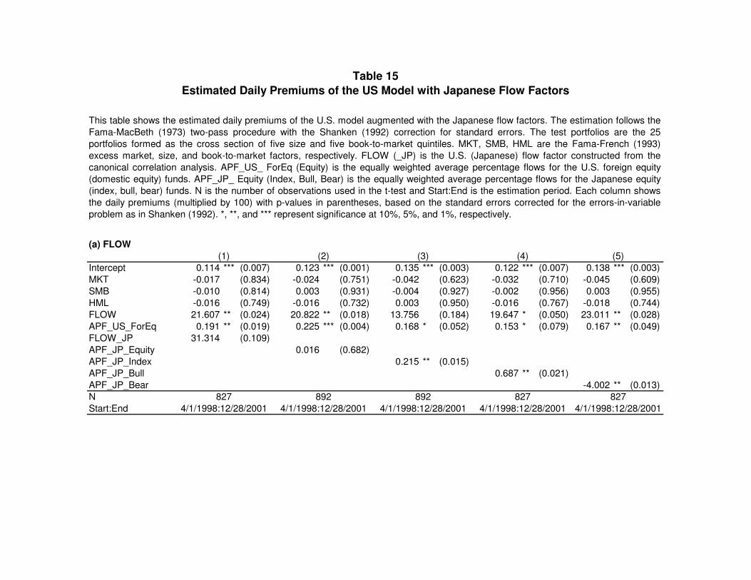
Table 15

Estimated Daily Premiums of the US Model with Japanese Flow Factors

(a) FLOW

(1) (2) (3) (4) (5)

Intercept 0.114 *** (0.007) 0.123 *** (0.001) 0.135 *** (0.003) 0.122 *** (0.007) 0.138 *** (0.003)

MKT -0.017 (0.834) -0.024 (0.751) -0.042 (0.623) -0.032 (0.710) -0.045 (0.609)

SMB -0.010 (0.814) 0.003 (0.931) -0.004 (0.927) -0.002 (0.956) 0.003 (0.955)

HML -0.016 (0.749) -0.016 (0.732) 0.003 (0.950) -0.016 (0.767) -0.018 (0.744)

FLOW 21.607 ** (0.024) 20.822 ** (0.018) 13.756 (0.184) 19.647 * (0.050) 23.011 ** (0.028)

APF_US_ForEq 0.191 ** (0.019) 0.225 *** (0.004) 0.168 * (0.052) 0.153 * (0.079) 0.167 ** (0.049)

FLOW_JP 31.314 (0.109)

APF_JP_Equity 0.016 (0.682)

APF_JP_Index 0.215 ** (0.015)

APF_JP_Bull 0.687 ** (0.021)

APF_JP_Bear -4.002 ** (0.013)

N 827 892 892 827 827

Start:End 4/1/1998:12/28/2001 4/1/1998:12/28/2001 4/1/1998:12/28/2001 4/1/1998:12/28/2001 4/1/1998:12/28/2001

This table shows the estimated daily premiums of the U.S. model augmented with the Japanese flow factors. The estimation follows the

Fama-MacBeth (1973) two-pass procedure with the Shanken (1992) correction for standard errors. The test portfolios are the 25

portfolios formed as the cross section of five size and five book-to-market quintiles. MKT, SMB, HML are the Fama-French (1993)

excess market, size, and book-to-market factors, respectively. FLOW (_JP) is the U.S. (Japanese) flow factor constructed from the

canonical correlation analysis. APF_US_ ForEq (Equity) is the equally weighted average percentage flows for the U.S. foreign equity

(domestic equity) funds. APF_JP_ Equity (Index, Bull, Bear) is the equally weighted average percentage flows for the Japanese equity

(index, bull, bear) funds. N is the number of observations used in the t-test and Start:End is the estimation period. Each column shows

the daily premiums (multiplied by 100) with p-values in parentheses, based on the standard errors corrected for the errors-in-variable

problem as in Shanken (1992). *, **, and *** represent significance at 10%, 5%, and 1%, respectively.

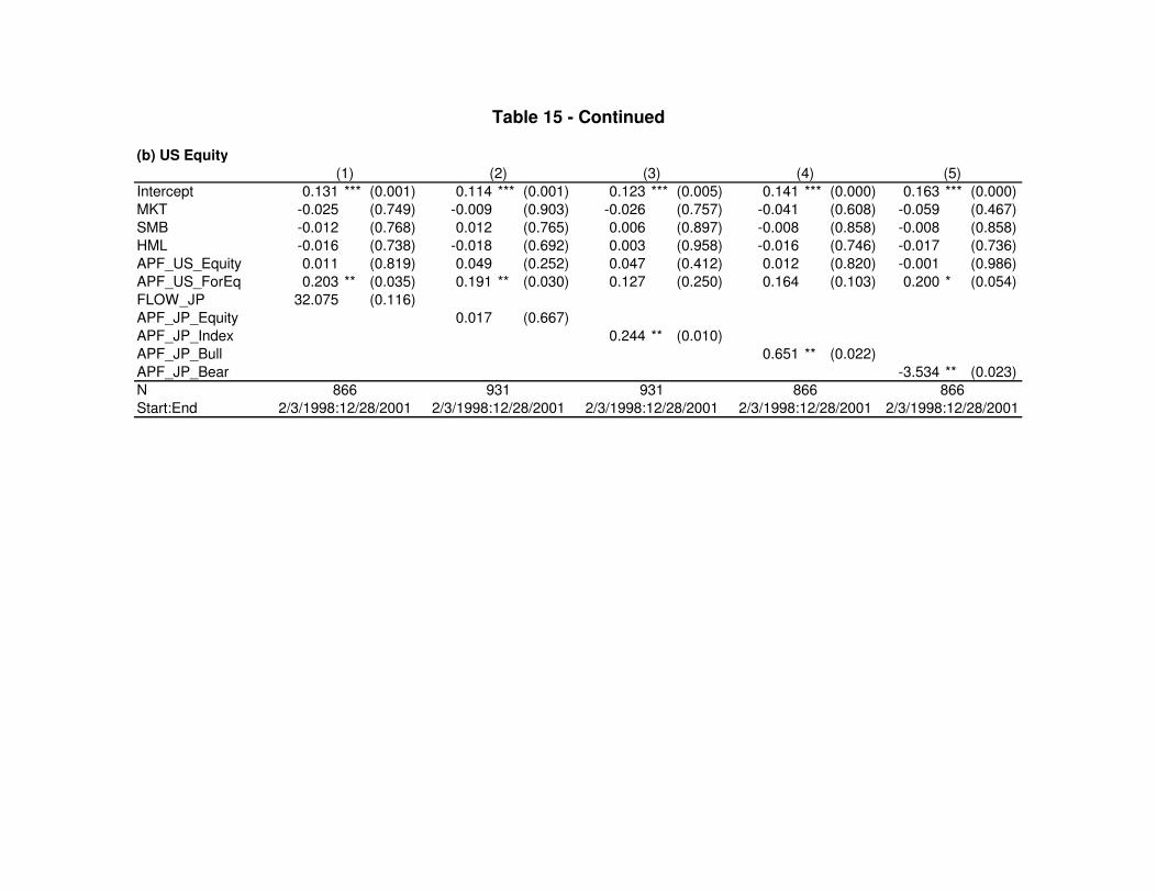
Table 15 - Continued

(b) US Equity

(1) (2) (3) (4) (5)

Intercept 0.131 *** (0.001) 0.114 *** (0.001) 0.123 *** (0.005) 0.141 *** (0.000) 0.163 *** (0.000)

MKT -0.025 (0.749) -0.009 (0.903) -0.026 (0.757) -0.041 (0.608) -0.059 (0.467)

SMB -0.012 (0.768) 0.012 (0.765) 0.006 (0.897) -0.008 (0.858) -0.008 (0.858)

HML -0.016 (0.738) -0.018 (0.692) 0.003 (0.958) -0.016 (0.746) -0.017 (0.736)

APF_US_Equity 0.011 (0.819) 0.049 (0.252) 0.047 (0.412) 0.012 (0.820) -0.001 (0.986)

APF_US_ForEq 0.203 ** (0.035) 0.191 ** (0.030) 0.127 (0.250) 0.164 (0.103) 0.200 * (0.054)

FLOW_JP 32.075 (0.116)

APF_JP_Equity 0.017 (0.667)

APF_JP_Index 0.244 ** (0.010)

APF_JP_Bull 0.651 ** (0.022)

APF_JP_Bear -3.534 ** (0.023)

N 866 931 931 866 866

Start:End 2/3/1998:12/28/2001 2/3/1998:12/28/2001 2/3/1998:12/28/2001 2/3/1998:12/28/2001 2/3/1998:12/28/2001

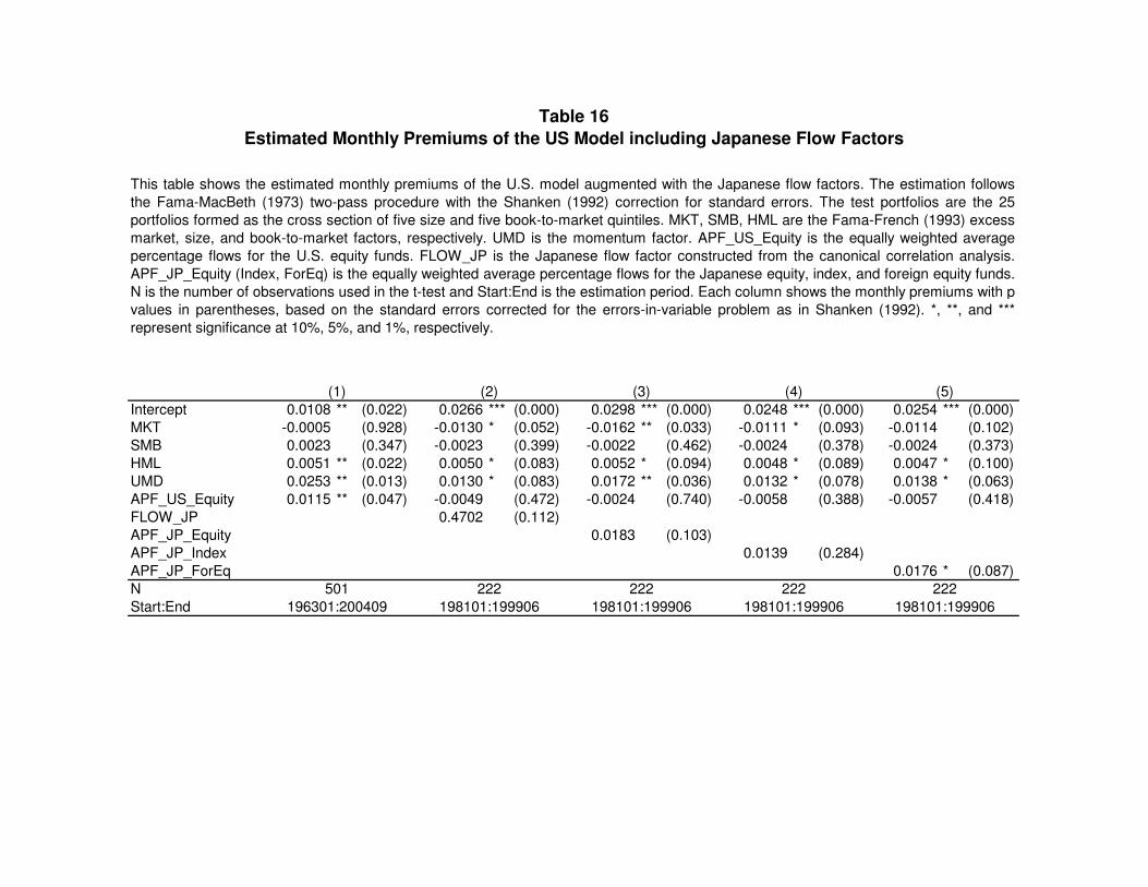
Table 16

Estimated Monthly Premiums of the US Model including Japanese Flow Factors

(1) (2) (3) (4) (5)

Intercept 0.0108 ** (0.022) 0.0266 *** (0.000) 0.0298 *** (0.000) 0.0248 *** (0.000) 0.0254 *** (0.000)

MKT -0.0005 (0.928) -0.0130 * (0.052) -0.0162 ** (0.033) -0.0111 * (0.093) -0.0114 (0.102)

SMB 0.0023 (0.347) -0.0023 (0.399) -0.0022 (0.462) -0.0024 (0.378) -0.0024 (0.373)

HML 0.0051 ** (0.022) 0.0050 * (0.083) 0.0052 * (0.094) 0.0048 * (0.089) 0.0047 * (0.100)

UMD 0.0253 ** (0.013) 0.0130 * (0.083) 0.0172 ** (0.036) 0.0132 * (0.078) 0.0138 * (0.063)

APF_US_Equity 0.0115 ** (0.047) -0.0049 (0.472) -0.0024 (0.740) -0.0058 (0.388) -0.0057 (0.418)

FLOW_JP 0.4702 (0.112)

APF_JP_Equity 0.0183 (0.103)

APF_JP_Index 0.0139 (0.284)

APF_JP_ForEq 0.0176 * (0.087)

N 501 222 222 222 222

Start:End 196301:200409 198101:199906 198101:199906 198101:199906 198101:199906

This table shows the estimated monthly premiums of the U.S. model augmented with the Japanese flow factors. The estimation follows

the Fama-MacBeth (1973) two-pass procedure with the Shanken (1992) correction for standard errors. The test portfolios are the 25

portfolios formed as the cross section of five size and five book-to-market quintiles. MKT, SMB, HML are the Fama-French (1993) excess

market, size, and book-to-market factors, respectively. UMD is the momentum factor. APF_US_Equity is the equally weighted average

percentage flows for the U.S. equity funds. FLOW_JP is the Japanese flow factor constructed from the canonical correlation analysis.

APF_JP_Equity (Index, ForEq) is the equally weighted average percentage flows for the Japanese equity, index, and foreign equity funds.

N is the number of observations used in the t-test and Start:End is the estimation period. Each column shows the monthly premiums with p-

values in parentheses, based on the standard errors corrected for the errors-in-variable problem as in Shanken (1992). *, **, and ***

represent significance at 10%, 5%, and 1%, respectively.

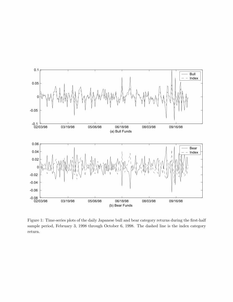
02/03/98 03/19/98 05/06/98 06/18/98 08/03/98 09/16/98-0.1

-0.05

0

0.05

0.1

(a) Bull Funds

BullIndex

02/03/98 03/19/98 05/06/98 06/18/98 08/03/98 09/16/98-0.08

-0.06

-0.04

-0.02

0

0.02

0.04

0.06

(b) Bear Funds

BearIndex

Figure 1: Time-series plots of the daily Japanese bull and bear category returns during the first-halfsample period, February 3, 1998 through October 6, 1998. The dashed line is the index categoryreturn.