Investor Sentiment, Beta, and the Cost of Equity Capital

Constantinos Antoniou, John A. Doukas, and Avanidhar Subrahmanyam

*

September 28, 2014

Abstract The security market line (SML) accords with the capital asset pricing model (CAPM) by taking on an

upward slope in pessimistic sentiment periods, but is downward sloping during optimistic periods. We

hypothesize that this finding obtains because periods of optimism attract equity investment by

unsophisticated, overconfident, traders in risky opportunities (high beta stocks), while such traders stay

along the sidelines during pessimistic periods. Thus, high beta stocks become overpriced in optimistic

periods, but during pessimistic periods, noise trading is reduced, so that traditional beta pricing prevails.

Unconditional on sentiment, these effects offset each other. While rational explanations cannot

completely be ruled out, analyses using earnings expectations, fund flows, the probability of informed

trading, and order imbalances do provide evidence that noise traders are more bullish about high beta

stocks when sentiment is optimistic, while investor behavior appears to accord more closely with

rationality during pessimistic periods, supporting our hypothesis.

* Antoniou, constantinos.antoniou@wbs.ac.uk, Warwick Business School, University of Warwick, Gibbet

Hill Road, Coventry, CV4 7AL, U.K., Tel: 44-(1392) 726256. Doukas, doukas@odu.edu, Old Dominion

University, Strome College of Business, Constant Hall, Suite 2080, Norfolk, VA 23529-0222, Tel: 1-

(757) 683-5521, and Judge Business School, University of Cambridge, U.K. Subrahmanyam

(corresponding author), subra@anderson.ucla.edu, Nanjing University School of Management and

Engineering, and the Anderson School, University of California, Los Angeles, CA 90095-1481, Tel: 1-

(310) 825-5355. We are grateful to Wei Jiang (the editor), an anonymous Associate Editor, and two

anonymous referees, for their insightful and constructive feedback. We also thank Malcolm Baker, Peter

DaDalt, Pasquale Della Corte, Arie Gozluklu, Tony Hewitt, Rustam Ibragimov, Roman Kozhan, Yul Lee,

Anthony Neuberger, Vikas Raman, Raghu Rau, Richard Taffler, Julian Xu, Pedro Saffi, James Sefton,

Katrin Tinn, Tong Yu, Paolo Zaffaroni, and seminar participants at the University of Cambridge, Center

of Planning and Economic Research (Athens, Greece), Imperial College, University of Reading,

University of Rhode Island, and the University of Warwick for useful comments and suggestions.

1

The CAPM of Sharpe (1964), Lintner (1965) and Mossin (1966) posits that if traders are rational and

sophisticated, expected returns increase linearly with asset betas, and is an integral element of capital

budgeting decisions. In a seminal study, however, Fama and French (1992) show that beta is unrelated to

returns, casting doubt on the applicability of the CAPM. Various explanations have been put forward to

explain this puzzle ranging from mispecifications of risk (Jagannathan and Wang, 1996), to inefficiency

of market proxies (Roll and Ross, 1994) to frictions (Black, 1972; Baker, Bradley and Wurgler, 2011). In

this paper, we examine the relation between beta pricing and variations in the degree of unsophisticated

trading due to the dynamics of investor sentiment.

The phrase “sentiment” refers to whether or not an agent possesses excessively positive or

negative affect, and evidence from research in decision sciences shows that positive sentiment results in

overly optimistic views, and vice versa (Bower, 1981, 1991; Arkes, Herren, and Isen, 1988; Wright and

Bower, 1992; Johnson and Tversky, 1992).1 In financial markets, optimistic or pessimistic beliefs induced

by sentiment should trigger unsophisticated (“noise”) trading, as postulated by Black (1986), and thus

affect financial asset prices. However, there are reasons to believe that such trading will not be symmetric

across optimistic and pessimistic sentiment periods, but will be more prevalent during optimistic ones.

For example, as shown by Amromin and Sharpe (2009), individual investors expect higher stock returns,

and thus participate in equities more strongly, following good periods rather than following bad ones.

Similarly Grinblatt and Keloharju (2001) and Lamont and Thaler (2003) find that unsophisticated

investors are more likely to enter the stock market during prosperous periods. Taken together, these

arguments suggest that unsophisticated trading will be more prevalent and impactful in optimistic

periods.2

We argue that the heightened noise trader activity in optimistic periods will not affect all

companies equally, but will be disproportionately concentrated among high beta stocks. The general

1 For related work in experimental economics on the effect of sentiment on financial decisions see Kuhnen and

Knutson (2011) and Andrade, Odean and Lin (2012). 2 Furthermore, pessimistic investors need to engage in short selling to express their views and empirical evidence

show that individual investors are generally reluctant to sell short (Barber and Odean, 2008). This aversion to short

selling can also contribute to decreased noise trading in pessimistic sentiment periods.

2

preference of individual investors toward high beta stocks has been documented by Barber and Odean

(2000), who show that the market beta of the aggregate retail investors’ portfolio exceeds unity. Further,

Barber and Odean (2001, Table III) show that this preference is particularly strong among unsophisticated

retail investors (i.e., those who trade the most and earn the lowest returns--young, single males). These

observations indicate that the enhanced unsophisticated trading during optimistic periods would be more

prevalent in high beta stocks. Further, if unsophisticated traders are optimistic about the aggregate stock

market but face leverage constraints or are simply averse to borrowing or shorting, high beta stocks are a

natural vehicle for them to act on this optimism.

The above arguments can have implications regarding the validity of the CAPM. Specifically, if it

is indeed the case that unsophisticated traders are active market participants during optimistic periods, and

are attracted to high beta companies, they will overprice high beta stocks. If these investors, on the other

hand, stay by the sidelines during pessimistic periods, then the behavior of financial markets may be more

in line with neoclassical asset pricing theories, and beta will be positively related to returns. On the whole

these effects can cancel out, flattening the unconditional beta-return relationship. We provide empirical

support for the above arguments, by showing that the upward sloping security market line in pessimistic

(but not optimistic) periods is also accompanied by lower levels of unsophisticated trading in high beta

stocks during such periods.

In our base analysis, we use the Baker and Wurgler (2006) index (BW) to capture sentiment,

which is orthogonalized with respect to a set of macro variables. Confirming Stambaugh, Yu, and Yuan

(2012, Tables 7 and 8),3 we find that for the period 1966 to 2010, using the Fama and French (1992)

methodology, a standard beta, while unconditionally insignificant, is positively related to returns during

pessimistic periods, while estimates of the market risk premium are reasonable and in line with intuition.

Consistent with our prediction, the nullification of the beta-return relation stems from optimistic periods,

3 Stambaugh, Yu, and Yuan (2012) test whether the explanatory power of various cross-sectional predictors, not

explained by the Fama and French (1993) three factor model, vary with sentiment, and also present some evidence

in relation to the beta-return relationship. However, they do not examine the sources of the flat beta-return relation,

which represents an empirical failure of the CAPM.

3

where beta is negatively related to returns.

Next, we conduct several tests to examine whether the negative pricing of beta in optimistic

periods reflects an overpricing due to optimistic noise traders, who are attracted to high beta stocks. First,

since mutual fund flows reflect active reallocation decisions of individual investors, we examine whether

optimistic periods are associated with higher capital flows into equity mutual funds. Our results confirm

this prediction.

We then examine whether unsophisticated (noise) trading rises disproportionately for higher beta

stocks in optimistic periods, using different firm-level proxies for noise trading. Our first measure is the

signed forecast error in sell-side analyst earnings forecasts. Since sell-side analysts exert a powerful

impact on retail investor earnings expectations (Malmendier and Shanthikumar, 2007), their relative

optimism about high beta stocks can be used to capture the bullishness of noise traders. Secondly, we use

the Frazzini and Lamont (2008) flow-based measure that captures whether a specific stock is in

abnormally high demand by mutual fund investors. Lastly, we use the probability of informed trading (the

PIN measure of Easley, Hvidkjaer, and O’Hara 2002), as calculated in Brown and Hillegeist (2007),

which indicates whether the trading for a specific stock in a given month is likely to be driven by

fundamental information. Our results across all three measures consistently show that noise traders are

indeed relatively more bullish and active for high beta stocks when sentiment is optimistic, in line with

our hypothesis.

Several studies show that small trades are likely to reflect the trading decisions of noise traders

(Hvidkjaer, 2006; 2008; Malmendier and Shanthikumar, 2007). Along these lines, we use intra-day

transactions data to estimate stock-by-stock small trader order imbalances (SOIB), and test whether they

indicate more bullishness about high beta stocks in periods of optimism. We find that in optimistic

periods small investors are net buyers (sellers) of high (low) beta stocks, whereas no pattern is observed

in pessimistic periods. Moreover, when examining SOIB around earnings announcements and analyst

forecasts, we find that small investors are relatively more bullish (or less bearish) about high beta stocks

when sentiment is optimistic. The SOIB’s from pessimistic periods in response to these events show little

4

variation across beta portfolios, which suggests that in these periods rational investors largely anticipate

these announcements. Overall these results provide further support to our hypothesis.

Since our argument is that increased noise trading in optimistic sentiment periods leads to the

underperformance of high beta stocks, by augmenting the BW sentiment index to include information

from our proxies of noise trading, we should be better able to capture periods in which high beta stocks

are overpriced. To test this notion we perform principal component analysis using the BW sentiment

index and our proxies for noise trading, and define sentiment using the first principal component from this

procedure. We find that the augmented index is a more powerful predictor of the underperformance of

high beta stocks in optimistic periods compared to the original BW index, whereas both indices perform

similarly in pessimistic periods. This finding supports our hypothesis that heightened noise trading

activity leads to negative beta pricing in optimistic sentiment periods.

Finally, we conduct several double portfolio sorts, to examine whether the beta-return relation we

document reflects (or relates to) broader facets of firm risk. Specifically, we consider institutional

ownership (higher institutional ownership implies lower agency risk, viz. Gillian and Starks, 2000),

analyst coverage (high coverage stocks have lower information quality risk in the sense of Arbel and

Strebel, 1983), and short ratio (stocks with a higher proportion of shares held short in relation to total

shares outstanding are most likely cheaper to short sell and thus involve less noise trader risk, viz.

Shleifer and Summers, 1990). Our results indicate that positive beta pricing in pessimistic periods is

preserved in all tables, which suggests that it reflects pricing of covariance risk. Conversely, the negative

pricing of beta in optimistic periods, is stronger among stocks with lower analyst coverage and stocks

which are more expensive to sell short, which, suggests that the negative pricing of beta in optimistic

periods arises from investors’ behavioral biases and limits to arbitrage.

Our results hold when we account for the predictability of market returns from sentiment, if we

measure sentiment using the Consumer Confidence Index compiled by the University of Michigan, to

different beta specifications, to controls for additional variables and to previous determinants of a time-

varying security market line (SML). We discuss these robustness tests in later sections of the paper.

5

Of course, there is always the possibility that the Baker and Wurgler (2006) measure of sentiment

captures a state variable related to macroeconomic risk, and that beta and its pricing dynamically vary

with this state variable. While this possibility cannot completely be ruled out, Lewellen and Nagel

(2006) argue that variation in conditional betas would need to be implausibly large to explain asset

pricing anomalies.4 Further, in our context, a rational argument would also need to explain why a

traditional beta is negatively priced during optimistic periods, which seems like a daunting task. Finally,

as we mention in Section 7 to follow, we find that our results continue to hold when we use betas

conditional on sentiment. Thus, we believe that, if rational channels play a role in our findings, it is likely

that they do so in conjunction with behavioral channels.

In other related work, Yu and Yuan (2011) report that the positive relationship between aggregate

market volatility and market returns only exists in pessimistic periods. In independent work, Shen and Yu

(2012) argue that stocks with high exposure to macroeconomic shocks carry a positive premium in

pessimistic periods (see also Jouini and Napp (2011)). Investor sentiment has been linked to various cross

sectional predictors of stock returns (Livnat and Petrovic, 2008; Antoniou, Doukas, and Subrahmanyam,

2013; Cen, Lu and Yang, 2013; Stambaugh, et al., 2012). Thus, existing literature has linked sentiment to

both the rational risk-return tradeoff and anomalies left unexplained by rational pricing models.

Our results add to the growing literature on how sentiment affects equity prices and influences

thinking on the behavioral versus neoclassical finance debate. Since the seminal result of Fama and

French (1992) that the empirical return-beta relation is flat,5 various explanations have been put forward

for why beta is not priced, such as the inefficiency of market proxies (Roll and Ross, 1994), the inability

of standard unconditional tests to properly measure systematic risk (Jagannathan and Wang, 1996; Lettau

and Ludvigson, 2001), delegated portfolio management (Karceski, 2002; Brennan, Cheng, and Li, 2012),

4 Specifically, Lewellen and Nagel (2006) show that if a conditional CAPM holds, a stock’s alpha depends primarily

on the covariance between beta and the market risk premium, which is bounded above by the product of the standard

deviations of beta and the premium. The empirical standard deviations are not nearly high enough to explain the

alphas achieved from predictor variables corresponding to common asset pricing anomalies. 5 Early investigations of the relation between average returns and covariance risk met with mixed results; see, for

example, Douglas (1969), Black, Jensen, and Scholes (1972), Fama and MacBeth (1973), and Haugen and Heins

(1975).

6

market frictions (Black, 1972; Baker, Bradley and Wurgler, 2011; Frazzini and Pedersen, 2014) and the

omission of state variables (Acharya and Pedersen 2005; Campbell et al., 2012).

Other literature has also produced evidence that the slope of the SML is time varying. Cohen,

Polk, and Vuolteenaho (2005) advance an argument based on money illusion, and show that riskier stocks

earn higher returns when expected inflation is low. Similarly, Hong and Sraer (2012) propose that the

underperformance of risky stocks relates to aggregate disagreement about the market factor and limits to

arbitrage, and Frazzini and Pedersen (2014) show that in periods of tighter borrowing constraints the

security market line is flatter. In our analysis we find that, whilst controlling for these predictors of the

SML’s slope, investor sentiment influences the beta-return relation, in line with the notion of noise

trading, as advanced by Black (1986).

1. Hypotheses

Our hypotheses are based on the dual premises that pessimistic periods consist of rational investors and

optimistic periods attract unsophisticated investors. We thus propose that capital market equilibria are

different across optimistic and pessimistic periods.

The studies cited in the introduction (Amromin and Sharpe, 2009; Grinblatt and Keloharju, 2001;

Lamont and Thaler, 2003) all suggest that individual investors may be more prone to investing in risky

assets during optimistic periods. We thus propose that unsophisticated investors stay by the sidelines

during pessimistic periods, so that these periods consist of utility-maximizing risk averse agents. This

implies that a standard CAPM holds during these periods.

We propose periods of optimism attract unsophisticated agents who hold unduly optimistic

beliefs about market returns. We argue that these agents exploit their signal only in high beta stocks. We

motivate this assumption as follows. Barber and Odean (2000) show that the typical retail investor’s

portfolio is tilted toward higher beta stocks (they document a loading of 1.1 of the aggregate retail

investor portfolio on the market factor). Further, Barber and Odean (2001) show that the most

unsophisticated investors (young, single males, who lose the most from investing, and are the most

susceptible to overconfidence), also prefer to be long on riskier (higher beta) stocks. We note that if

7

optimistic investors are averse to shorting or borrowing, they would prefer to buy stocks with high

exposure to the market, as these promise higher perceived benefits from trading.

Under the condition that the optimism of unsophisticated traders is expressed primarily in high

beta stocks, such stocks will become overvalued during optimistic periods.6 All of the above arguments

lead to the following hypotheses:

H1. Under optimistic periods, stocks with high betas are overpriced. Specifically, the expected return

difference between high- and low-beta stocks is negative.

H2. During pessmistic periods, a standard CAPM obtains, so that beta is positively priced.

Hypotheses H1 and H2 above form the bases for our empirical analyses. First, we investigate

whether high beta stocks have lower returns in optimistic periods, and higher returns in pessimistic

periods. Second, we examine whether noise traders are more bullish for high beta stocks in optimistic

periods.

2. Data and Methodology

2.1 Sentiment Index

We measure sentiment using the annual index provided by Baker and Wurgler (2006). This index is

constructed using six proxies of investors’ propensity to invest in stocks: trading volume (total NYSE

turnover), the premium for dividend paying stocks, the closed-end fund discount, the number and first-

day returns of IPOs, and the equity share in new issues. To remove the effect of economic fundamentals

from these variables, Baker and Wurgler (2006) regress each of them on growth in industrial production,

real growth in durable consumption, non-durable consumption, services consumption, growth in

employment, and an NBER recession indicator, and use the first principal component of the residuals

from the regressions as the Sentiment Index. 7, 8

We define all observations in year t as optimistic

6 Simple analytical frameworks demonstrating these points are available upon request. We thank the Associate

Editor for suggesting another mechanism: Unsophisticated investors may be overconfident about a (valid) positive

market signal during optimistic periods, and overinvest in high beta stocks, as leverage constraints might preclude a

large investment in the market index. This phenomenon would also lead to overvaluation of high beta stocks. 7 We thank Malcolm Baker and Jeffrey Wurgler for making the Sentiment Index publicly available.

8

(pessimistic) if the Sentiment Index is positive (negative) in year t-1 (Yu and Yuan, 2011). The index is

available from 1965 to 2010, so our sample covers the period 1966-2010.

2.2 Asset pricing regressions

In our empirical tests we use all common stocks (share codes 10 and 11) listed on the NYSE, AMEX, and

NASDAQ for which we have available data for each of the ensuing tests. Prices, returns, and shares

outstanding are from the CRSP monthly files, while book values of equity are obtained from Compustat

(as in Fama and French, 1992).

We start by estimating beta following the methodology of Fama and French (1992). Specifically,

in June of year t, all NYSE firms are sorted by size (price x shares outstanding) to determine decile

breakpoints. Using these breakpoints, we assign all firms in the sample in year t to 10 size portfolios. To

allow for variation in beta that is unrelated to size, we further subdivide each size decile into 10 portfolios

sorted on pre-ranking betas for individual stocks. These pre-ranking betas are calculated using 24 to 60

monthly returns (as available) ending in June of year t. We set beta breakpoints for each size decile using

only NYSE stocks. This procedure yields 100 size-beta portfolios.

After assigning firms into size-beta portfolios in June, we obtain the equally-weighted returns of

these portfolios from July of year t until June of year t+1. This yields 100 time series of returns, one for

each size-beta portfolio, spanning our entire sample period. We estimate post-formation betas using the

returns of these portfolios and the CRSP value-weighted return as a proxy for the market portfolio. As in

Fama and French (1992), pre- and post-ranking betas are calculated as the sum of the slopes in the

regression of returns on the current and lagged market return. These betas are then assigned back to

individual stocks, depending on their size-beta classification. To make sure that all the information used

to explain returns is known ex ante, we mainly focus on rolling betas using five years of data prior to the

holding period in month t. However, we present results using the full sample betas in Section 6.2 to

8 In recent and independent work, Sibley, Xing, and Zhang (2012) show that the Baker and Wurgler index correlates

with contemporaneous business cycle variables, but they do not rule out the possibility that these variables may also

capture sentiment. They also show that including the sentiment variable reduces pricing errors for 25 size and

book/market-sorted portfolios relative to the Fama and French (1992) three-factor model. Unlike us, they do not

focus on cross-sectional beta pricing across individual stocks.

9

follow.

Our main analysis employs the Fama and MacBeth (1973) methodology. Thus, in each month t

we run a cross-sectional regression of returns on post-formation betas and control variables. The time

series average of the regression coefficients and its standard error provide standard tests of whether these

variables are on average priced in the cross-section of stock returns. In the cross-sectional regressions, we

control for firm size (Banz, 1981), the book/market ratio of equity (Statman, 1980), the return of stock i in

month t-1 (Jegadeesh, 1990), the cumulative return of stock i in the six months prior to month t-1

(Jegadeesh and Titman, 1993), and the cumulative return of stock i in the six months prior to month t-7

(Novy-Marx, 2012).

2.3 Summary statistics

Table 1 shows the time series averages of the post-formation rolling betas for each size-beta portfolio,

with three important findings emerging. First, post-ranking betas precisely reproduce the ranking of pre-

ranking betas, second, there is sizable variation in betas that is unrelated to firm size, and third, betas are

generally larger for smaller companies.

Table 2 shows some key characteristics of the beta-sorted portfolios. High-beta stocks tend to be

smaller stocks with lower B/M ratios and return on assets, as well as higher total volatility and dispersion

in analysts’ earnings forecasts (i.e., analyst disagreement). These results are consistent with the notion

that high-beta stocks tend to be riskier companies with more speculative cash flows.

Table 3 provides descriptive statistics and pooled time series, cross-sectional, correlation

coefficients for betas (rolling and full sample) and the control variables in Panels A and B, respectively. It

can be seen that the summary statistics of the rolling and full sample betas are fairly similar. The mean

and median values of the logarithm of firm size and the book-to-market ratio are close to each other,

suggesting little skewness. Panel B of Table 3 indicates that the correlation between the rolling and full

sample betas exceeds 80%. Overall, the correlations are quite modest suggesting that multicollinearity is

not likely a material issue in our statistical tests.

3. Portfolio Results

10

We begin with a simple portfolio test. We rank stocks based on their pre-formation betas in deciles (using

NYSE breakpoints) in June of year t and hold these portfolios for 12 months. We calculate their returns in

each month t on a value-weighted basis. The time series averages of the monthly value-weighted returns

for the beta portfolios are presented in Table 4. To label periods as optimistic or pessimistic, we follow

the procedure outlined in the previous section, and average these monthly returns separately for optimistic

and pessimistic months.

The first row of Table 4 presents unconditional results for our entire sample period. The results

corroborate the findings of Fama and French (1992), who report that the relationship between beta and

returns is flat. The difference in average monthly returns between the extreme beta deciles is a trivial -

0.01% and is not statistically significant. The second row of Table 4 presents the average monthly return

of these portfolios in pessimistic sentiment months and indicates that stock returns increase with beta, as

predicted by the CAPM. The average monthly return of the low-beta portfolio is 0.79% and is 1.88% in

the high-beta portfolio. This is a return spread of more than 12% per year. A t-test for whether the return

of the high-beta portfolio is greater than that of the low-beta portfolio, as predicted by theory, produces a

p-value smaller than 5%. Figure 1 shows a graphical illustration of this result by demonstrating the

upward-sloping nature of the empirical SML during pessimistic periods.9

The third row in Table 4 shows the average monthly returns of the beta portfolios in optimistic

sentiment periods. In these periods low-beta stocks outperform high-beta stocks. According to our

hypothesis this occurs because noise traders overprice high beta stocks when they are optimistic. We

conduct several tests to directly test this proposition in Section 5.

4. Regression Analysis

The results in the previous section are indicative of a positive relationship between beta and stock returns

in pessimistic periods. In this section, we provide more direct evidence using the regression approach of

Fama and MacBeth (1973). As discussed earlier, we also control for various other characteristics that

9 We have verified that our results continue to hold if we terminate the analysis in 2006, and thus eliminate the

financial crisis of 2007 and beyond. These results are available upon request.

11

have been shown to affect returns.

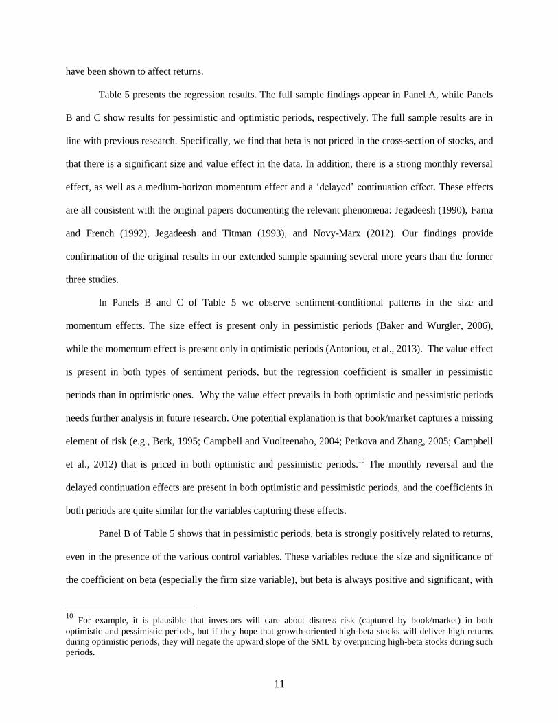
Table 5 presents the regression results. The full sample findings appear in Panel A, while Panels

B and C show results for pessimistic and optimistic periods, respectively. The full sample results are in

line with previous research. Specifically, we find that beta is not priced in the cross-section of stocks, and

that there is a significant size and value effect in the data. In addition, there is a strong monthly reversal

effect, as well as a medium-horizon momentum effect and a ‘delayed’ continuation effect. These effects

are all consistent with the original papers documenting the relevant phenomena: Jegadeesh (1990), Fama

and French (1992), Jegadeesh and Titman (1993), and Novy-Marx (2012). Our findings provide

confirmation of the original results in our extended sample spanning several more years than the former

three studies.

In Panels B and C of Table 5 we observe sentiment-conditional patterns in the size and

momentum effects. The size effect is present only in pessimistic periods (Baker and Wurgler, 2006),

while the momentum effect is present only in optimistic periods (Antoniou, et al., 2013). The value effect

is present in both types of sentiment periods, but the regression coefficient is smaller in pessimistic

periods than in optimistic ones. Why the value effect prevails in both optimistic and pessimistic periods

needs further analysis in future research. One potential explanation is that book/market captures a missing

element of risk (e.g., Berk, 1995; Campbell and Vuolteenaho, 2004; Petkova and Zhang, 2005; Campbell

et al., 2012) that is priced in both optimistic and pessimistic periods.10

The monthly reversal and the

delayed continuation effects are present in both optimistic and pessimistic periods, and the coefficients in

both periods are quite similar for the variables capturing these effects.

Panel B of Table 5 shows that in pessimistic periods, beta is strongly positively related to returns,

even in the presence of the various control variables. These variables reduce the size and significance of

the coefficient on beta (especially the firm size variable), but beta is always positive and significant, with

10

For example, it is plausible that investors will care about distress risk (captured by book/market) in both

optimistic and pessimistic periods, but if they hope that growth-oriented high-beta stocks will deliver high returns

during optimistic periods, they will negate the upward slope of the SML by overpricing high-beta stocks during such

periods.

12

a t-statistic of at least 2.42.11

Although the implied market premium is quite high when beta is the only

variable, it is brought down to 0.8%-0.9% per month when control variables are included in the cross-

sectional regression. While still higher than the 8.0%-8.5% annual premium documented in various

sources (e.g., Allen, Brealey, and Myers, 2010), this premium nonetheless is reasonable in terms of its

magnitude.12

In untabulated analysis we regress the time series coefficients on beta on a constant and the level

of sentiment in the previous year. We obtain a coefficient on sentiment equal to -0.52 with a Newey and

West (1987)-corrected t-statistic equal to -2.42, which shows that our result continues to hold when we

define sentiment as a continuous variable.

Panel C of Table 5 indicates that beta is negatively related to returns during optimistic periods.

We argue using formal tests in Section 5 that this is because during optimistic periods risky stocks

become overpriced and subsequently underperform.13

A t-test for the difference between the two

coefficients on beta across Panels B and C safely rejects the hypothesis that they are equal.14, 15

We

conduct several additional tests to establish the significance of this differential, which are available from

the authors upon request.

We would like to stress, however, an issue that is common to papers that use the sentiment index

of Baker and Wurgler (2006). Specifically, the sentiment index is a principal component extracted from

11

In additional analysis, we replicate the above regressions controlling for liquidity using the Amihud (2002)

measure [calculated using Equation (1) in Brennan, Huh, and Subrahmanyam (2013)]. To address issues arising

from different calculations of NYSE/AMEX and NASDAQ volume, we add two Amihud measures in the

regressions, IlliqNYAM (IlliqNas), which takes the value implied by this equation if the company is listed on NYSE

or AMEX (NASDAQ), and 0 otherwise. Because NASDAQ volume is not available prior to 1982, these tests are

based on a smaller sample; however, the results are virtually unchanged. 12

A risk premium of 8.5% is well within the one standard deviation band of our pessimistic period coefficient

including all controls. Note that the standard deviation of the risk premium we obtain is comparable to those

reported in Fama and MacBeth (1973) and Fama and French (1992). 13

Preliminary results are supportive, however, as we find that stocks in the optimistic period high-beta portfolio

outperform stocks in the low-beta portfolio in the period t-13 to t-36 by 62% (t-statistic = 5.77), where t is the

portfolio formation month (recall that optimism is defined based on the sentiment index in the past year). The

corresponding figure in pessimistic periods is 10% (t-statistic = 1.29). 14

The medians of the betas in optimistic and pessimistic periods are also significantly different. 15

Fama and MacBeth (1973) find evidence that support the CAPM for the pre-1970 period. In unreported analysis

we use the sentiment index provided by Baker and Wurgler that is available from 1934 (SENT^(old)), and perform

the tests in Table 5 conditional on sentiment for the period 1934-1965. Qualitatively we obtain similar findings in

relation to the pricing of beta as those in Table 5.

13

several time series, and as such, requires full sample information for construction. This implies that our

approach is not amenable to estimation in real time. It would be valuable for researchers and practitioners

if future research were to identify an alternative sentiment proxy based only on historical information.

5. Sentiment, Beta, and Noise Trading

While our baseline results show that high-beta stocks earn higher average returns than low-beta stocks in

pessimistic periods, the reverse happens in optimistic periods. According to our arguments, this occurs

because in optimistic periods noise traders are more bullish for high-beta stocks. This leads to an

overpricing of these stocks in optimistic periods, and therefore lower subsequent returns. In this section

we test this conjecture using several proxies that capture noise trader activity.

Our starting point is the notion that for (presumably unsophisticated) retail investors, the principal

avenue for broad-based stock market participation is through mutual funds.16

This implies that fund flows

can be used as a proxy for retail investor optimism, a point also made by earlier studies (Teo and Woo,

2004; Baker and Wurgler, 2007; Frazzini and Lamont, 2008). In untabulated analysis, we estimate

aggregate monthly fund flows (AFLOW) using the CRSP Mutual Fund Database and following the

procedure in Akbas et al. (2014, Eq. (3), p. 11).17

The results indicate that AFLOW is 0.61% in optimistic

months versus 0.39% in pessimistic months, and that the difference is statistically significant at the 5%

level. In dollar terms, mutual funds experience an average increase in inflows of $22 billion during

optimistic months relative to pessimistic ones. This analysis corroborates the view that there is increased

noise trader activity in optimistic periods.

We continue with tests that examine more directly whether noise traders are particularly bullish

about high beta stocks in periods of optimistic sentiment. Our first, and relatively direct, indicator, is a

measure of optimism in earnings expectations, measured by analysts’ signed earnings forecast errors.

16

The Investment Company Institute estimates that 44% of U.S. households owned mutual funds in 2011, and that

as a group households owned 89% of the mutual fund industry (2012 Investment Company Fact Book).

17 The equation is , where TNA is the total net assets of

fund i in month t and MRET is the return of fund i in month t.

, , 1 ,1,

, 11

( *(1 ))N

i t i t i tii t N

i ti

TNA TNA MRETMFFLOW

TNA

14

Hribar and McInnis (2012) show that analysts are susceptible to sentiment and produce more optimistic

earnings forecasts for uncertain stocks when sentiment is high. Given that analyst forecasts likely impact

retail investor expectations, “sentimental” analysts may also contribute to increased noise trading among

high-beta stocks in optimistic periods.18

Using the IBES summary files for one-year ahead forecasts we

calculate average forecast error (FE) for every firm in June of year t (defined as (mean forecast –

actual)/abs(actual)) and then take the average in the high- and low-beta portfolios conditional on

sentiment. Higher FE values indicate increased noise trading.

The results are shown in Panel A of Table 6. FE is generally higher for high beta stocks. This is

expected, since analyst bias is likely to be stronger in situations when uncertainty is higher. However, and

consistent with the analysis of Hribar and McInnis (2012), we find that the relative increase in FE is much

more pronounced in optimistic sentiment periods (0.11: t-stat 4.46). Moreover, we find that in optimistic

periods FE reduces for low beta stocks and increases for high beta stocks, and that these differentials are

statistically significant. This indicates higher relative noise trading among high beta stocks when

sentiment is optimistic.

Our next set of proxies capture the bullishness of noise traders toward high beta stocks through

their trading decisions. Frazzini and Lamont (2008) argue that stocks that are held by funds with a high

positive difference between actual and hypothetical flows can be thought of as being in demand among

noise traders, and are therefore overpriced. We thus compare actual with hypothetical flows into fund i in

quarter t, where hypothetical flows are recursively proportional to fund i’s TNA relative to the entire

mutual fund industry from three years ago. Stocks that are held by funds with a high positive difference

between actual and hypothetical flows (we label this difference FLOW) can be thought to be in demand

among noise traders, and are therefore overpriced.19

Using Equations (1)-(8) in Frazzini and Lamont

(2008), we calculate FLOW for each company every June of year t, and then take the average in the high

18

Note that excessively pessimistic forecasts are not likely to trigger noise trading because they are likely to be

uncommon, given the career concerns faced by sell-side analysts, viz. Hong and Kubik 2003). 19

To make these calculations, we use both the CRSP Mutual Funds Database and the CDA/Spectrum database

provided by Thomson Financial. For more details about this methodology, see Frazzini and Lamont (2008).

15

and low beta portfolios conditional on sentiment. In this table observations are divided into optimistic

(pessimistic) depending on whether the BW sentiment index is positive (negative) in year t. Higher

FLOW values indicate increased noise trading.

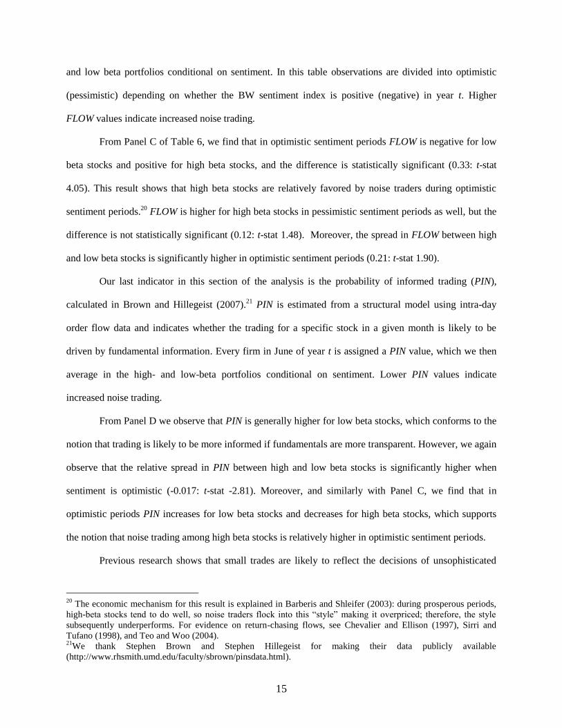
From Panel C of Table 6, we find that in optimistic sentiment periods FLOW is negative for low

beta stocks and positive for high beta stocks, and the difference is statistically significant (0.33: t-stat

4.05). This result shows that high beta stocks are relatively favored by noise traders during optimistic

sentiment periods.20

FLOW is higher for high beta stocks in pessimistic sentiment periods as well, but the

difference is not statistically significant (0.12: t-stat 1.48). Moreover, the spread in FLOW between high

and low beta stocks is significantly higher in optimistic sentiment periods (0.21: t-stat 1.90).

Our last indicator in this section of the analysis is the probability of informed trading (PIN),

calculated in Brown and Hillegeist (2007).21

PIN is estimated from a structural model using intra-day

order flow data and indicates whether the trading for a specific stock in a given month is likely to be

driven by fundamental information. Every firm in June of year t is assigned a PIN value, which we then

average in the high- and low-beta portfolios conditional on sentiment. Lower PIN values indicate

increased noise trading.

From Panel D we observe that PIN is generally higher for low beta stocks, which conforms to the

notion that trading is likely to be more informed if fundamentals are more transparent. However, we again

observe that the relative spread in PIN between high and low beta stocks is significantly higher when

sentiment is optimistic (-0.017: t-stat -2.81). Moreover, and similarly with Panel C, we find that in

optimistic periods PIN increases for low beta stocks and decreases for high beta stocks, which supports

the notion that noise trading among high beta stocks is relatively higher in optimistic sentiment periods.

Previous research shows that small trades are likely to reflect the decisions of unsophisticated

20

The economic mechanism for this result is explained in Barberis and Shleifer (2003): during prosperous periods,

high-beta stocks tend to do well, so noise traders flock into this “style” making it overpriced; therefore, the style

subsequently underperforms. For evidence on return-chasing flows, see Chevalier and Ellison (1997), Sirri and

Tufano (1998), and Teo and Woo (2004). 21

We thank Stephen Brown and Stephen Hillegeist for making their data publicly available

(http://www.rhsmith.umd.edu/faculty/sbrown/pinsdata.html).

16

traders (see for example, Hvidkjaer, 2006, 2008; and Malmendier and Shanthikumar, 2007). In this

section, we use intra-day transaction level data from the transaction and quotes database (TAQ) to

calculate small investor net order imbalance (SOIB), expecting to observe more bullishness for high beta

stocks in periods of optimism. To calculate order flow proxies for small investors we follow the

procedure in Hvidkjaer (2006).22

The results are shown in Table 7. In Panel A we calculate average daily SOIB for each firm-

month, and then report the rolling monthly average of high and low beta stocks ending in June of year t.

Observations are divided into optimistic (pessimistic) depending on whether the BW sentiment index is

positive (negative) in that year [this procedure is used for all analyses in Table 7]. We find that, in periods

of optimism, small investors are net buyers of high beta stocks and net sellers of low beta stocks (0.009

vs. -0.005, with the spread significant at the 10% level). No spread is observed between high and low beta

stocks in pessimistic periods. Moreover, when comparing the response of small investors toward high

beta stocks across sentiment periods, we find that small investors become net sellers in pessimistic

periods (-0.021), with the spread being statistically significant (0.03: t-stat -4.77). These results support

the notion that noise traders are attracted to high beta stocks in periods of optimism.

In Panels B-D we examine the response of small investors to earnings announcements, revisions

to analyst recommendations, and earnings forecasts. For earnings announcements we follow Livnat and

Mendenhall (2006) and calculate quarterly surprises using the seasonal random walk model. We assign

each event-firm in a beta portfolio using the beta classifications obtained in June of year t and rank firms

within each beta group in 4 standardized unexpected earnings (SUE) groups in each fiscal period. We

average daily small investor SOIB in the window [-1,0], where 0 is the announcement date, reporting

results for the low (SUE=1) and high (SUE=4) earnings surprise group. In Panels C and D we use annual

analyst earnings forecast revisions and revisions to analyst recommendations, which we classify into

22

The method involves using stocks size-based quintiles and computing the 99th stock price percentile. Small trades

are trades whose dollar values are less than defined as one hundred times this percentile, and large trades are defined

as those exceeding 200 times the percentile. Imbalances are market-adjusted by subtracting the market-wide

aggregate imbalance for each trade category.

17

upward and downward, repeating the analysis of Panel B.

From Panel B1 (SUE=4) we observe that small investors are significantly more bullish about high

beta stocks when sentiment is optimistic (-0.005 vs. 0.054). There is a similar, but weaker, effect in

pessimistic periods also (-0.047 vs. -0.007), and this effect is not statistically significant. Moreover, small

investors are net buyers of high beta stocks in optimistic periods, but net sellers in pessimistic periods

(0.054 vs. -0.023). Responses to negative surprises do not produce any significant results. In Panel C1, we

again observe that small investors are net buyers of high beta stocks, but net sellers for low beta stocks

during optimistic periods; but their behavior does not materially differ across high and low beta stocks

during pessimistic periods. From Panel C2 we also see that they are significantly less bearish about high

beta stocks after bad news (SUE=1) (-0.032 vs.-0.072). Finally, in Panel D1 we find that small investors

are net sellers for both high and low beta stocks, but less so for the former than the latter. The spreads in

SOIB between high and low beta stocks across sentiment periods are not significant in this table, but the

point estimates are generally consistent with our hypothesis. Collectively these results show that small

investors respond more favorably to information about high beta stocks than low beta stocks when they

are optimistic. On the contrary SOIB’s from pessimistic periods show little variation across beta

portfolios, which suggests rational investors largely anticipate the announcements or revisions.

Our next test examines whether noise traders are attracted to high beta stocks because they

allow market bets or because they are more speculative. To examine this we add into our Fama-MacBeth

regressions two additional variables that relate to firm uncertainty, namely disagreement, measured by

dispersion in analyst forecasts (Disp), and idiosyncratic volatility (IVOL). Diether, Malloy, and Scherbina

(DMS) (2002) show that stocks with high disagreement earn lower returns and argue that this reflects an

overpricing in the spirit of Miller (1977). Ang, Hodrick, Xing and Zhang (2006) (AHXZ) show that

stocks with high idiosyncratic volatility earn significantly lower returns. Gao, Yu, and Yuan (2012) show

this effect to be concentrated in optimistic sentiment periods, and suggest that it reflects an overpricing

due to noise trading activity.

The regression results with disagreement (Disp) and idiosyncratic volatility (IVOL) are shown in

18

Table 8. Note that analyst coverage data are only available from 1976 onwards, so the regressions that

include the two additional variables span a shorter sample period relative to Table 5 (ten less years than

the main sample, which begins in 1966). As in Table 5, we average the coefficients on the different

variables for the whole sample (Panel A), and separately for the Pessimistic (Panel B) and Optimistic

(Panel C) sentiment periods. Model 1 refers to a regression that includes the variables used in Table 5 for

this slightly shorter sample and Model 2 is the expanded version for this same sample, which also

includes disagreement and idiosyncratic volatility.

In Model 2 in Panel A of Table 8, we confirm DMS and AHXZ in that both Disp and IVOL are

unconditionally negatively related to returns. In addition, once we partition on sentiment, this effect is

concentrated in optimistic sentiment periods, consistent with the findings of Gao, Yu, and Yuan (2012).

Comparing Models 1 and 2 in Panel C, the inclusion of these variables reduces the coefficient on beta in

optimistic periods from -0.66% to -0.53% and its t-statistic from -2.03 to -1.68, which suggests that both

the aforementioned channels contribute to the negative pricing of beta in optimistic periods. As shown by

Panel B the beta-return relationship in pessimistic periods, is not affected, which suggests that in those

periods prices are set according to fundamentals.

Next, we test the notion that an augmented sentiment index using information from noise trading

proxies can better predict the underperformance of high beta stocks in optimistic periods. We use the

monthly sentiment index of Baker and Wurgler (2007) orthogonalized to macroeconomic variables in

month t, and the average Stock Specific Flow, FE and SOIB for high beta stocks (defined as in Tables 6

and 7b respectively) in the same month, perform principal component analysis, and retain the first

principal component as an augmented sentiment index.23

We average this augmented index for the months

t-1 to t-7, and if this rolling average is positive (negative) we define sentiment in month t as optimistic

(pessimistic). Using this index we repeat our baseline analysis in Tables 4 and 5. The time period for this

test is shorter, due to the fact that the noise trading proxies are not available for the earlier part of the

sample.

23

The correlation between this first principal component and the original sentiment index is 79%.

19

The results are shown in Table 9. Indeed we find that the augmented sentiment index is better

able to predict the negative pricing of beta in optimistic sentiment periods. From Panel A, in a portfolio

setting, we observe that the return spread between high and low beta stocks is -2.27% per month,

considerably larger than the -1.16% shown in Table 4. However, the spread in pessimistic periods is not

materially altered. In Panel B, in a Fama-MacBeth setting, we observe that the coefficient of beta in

optimistic sentiment periods with the augmented sentiment index is -1.27 (t-stat -3.04). When we repeat

this analysis for the same time period using the original Baker and Wurgler (2007) index we find that the

coefficient of beta is -0.70 (t-stat -2.02) (unreported result). Therefore, controlling for other variables, the

underperformance of high beta stocks reduces by 0.57% per month when the augmented index is used. In

pessimistic sentiment periods the coefficient on beta under the original sentiment index is 0.99 [t-stat

2.16], not very different from the coefficient of 0.87 [t-stat 2.38] shown in Table 9 Panel B. This finding

confirms that expanding the sentiment index to include information from the noise trading proxies

improves the capacity of the index to identify optimistic sentiment, and therefore predict the negative

pricing of beta in optimistic periods. The fact that the noise trading proxies do little to the predictability of

returns from beta in pessimistic sentiment periods suggests that in those periods noise trading is less

impactful and prices are set according to fundamentals.24

6. Beta-sorted Portfolios Cut Different Ways

In this section, we examine whether our central result is robust to firm characteristics that potentially

capture dimensions of risk other than beta. Our aim is to ascertain if beta pricing might be proxying for

some other risk source. Specifically, we consider institutional ownership (higher institutional ownership

firms can be thought to involve lower agency risk as institutions effectively monitor the CEO—viz.

Gillian and Starks, 2000), analyst coverage (high coverage stocks have lower information quality risk in

the sense of Arbel and Strebel, 1983), and short ratio (stocks with a higher proportion of shares held short

in relation to total shares outstanding are most likely cheaper to short sell and thus involve less noise

24

In unreported analysis we use the augmented sentiment index to replicate the analysis of Table 8 and Table 11,

and obtain very similar results as those in Table 9. These results are available from the authors on request.

20

trader risk-viz. Shleifer and Summers, 1990). We subdivide our sample into two groups using these

variables (High vs. Low, cutting at the median within each beta portfolio every June of year t), and

perform the portfolio analysis shown in Table 4 separately for each group. If beta pricing is proxying for a

missing risk characteristic, it should be less evident across high- and low-beta stocks within the high-risk

group (i.e., the low ownership, low coverage, and low short ratio groups).

The results of the portfolio analysis are shown in Table 10. Our main result of positive beta

pricing in pessimistic periods is preserved in all tables. Conversely, the result in optimistic periods, that

lower beta stocks outperform higher beta stocks, is much less stable and seems to be stronger among

higher uncertainty stocks, and stocks which are generally costlier to arbitrage. For example, as seen in

Panels B2 and C2, the underperformance of high-beta stocks is only observed among stocks with low

analyst coverage and those with low short ratio.25

7. Other Robustness Checks

In this section, we conduct a final set of tests to ascertain robustness of our results. First, we conduct the

Fama-MacBeth regressions from Table 8 (model 2) while controlling for additional variables shown in

Baker and Wurgler (2006) to affect stock returns conditional on sentiment. Specifically we include firm

age (AGE), external finance (EF), growth in sales (GS), and profitability and dividend paying dummies

(PrD, DivD, respectively). We define these variables following Baker and Wurgler (2006).

The results are shown in Table 11. For brevity we only report findings for pessimistic (Panel A)

and optimistic (Panel B) sentiment periods. We find that in pessimistic periods beta continues to be

positive and significant (0.67: t-stat 2.34), whereas in optimistic periods it is negative but insignificant (-

0.53; -1.49). In terms of the additional variables included in the regressions the results show that some

have explanatory power, in line with the results in Baker and Wurgler (2006), i.e., returns in optimistic

periods reduce with firm age and external finance, and returns in pessimistic periods are lower for

dividend paying stocks. Overall the results confirm that our findings are robust when controlling for a

25

We obtain similar results if, for each of the three partitioning variables, we perform a Fama-MacBeth style

regression with controls as in Table 5, using dummy variables to indicate the effect of beta on returns in the high and

low sub-groups.

21

comprehensive set of thirteen variables.

One issue is whether our differential results for beta pricing during optimistic and pessimistic

periods obtain because of variation in beta conditional on sentiment. To address this, we estimate

conditional betas using the technique of Jagannathan and Wang (1996), using the BW sentiment index as

the conditioning variable. The analysis indicates that these conditional betas are also positively priced in

pessimistic periods and negatively priced during optimistic periods. The results are not reported here for

brevity but are available upon request.

A concern with the rolling beta approach used in the main tests is that, due to the cyclicality of

sentiment, returns from past optimist periods are used to estimate betas, which are then related to returns

in pessimistic periods. It is possible, therefore, that betas may in fact encapsulate to some extent the

effects of past noise trading, and may not reflect pure systematic variation. In this section we perform two

tests to alleviate this concern. First, we use the methodology of Fama and French (1992) and calculate full

sample betas, which we assign to individual stocks. Arguably, the full sample betas will be less affected

by the noise trading since they are estimated in the full sample from both optimistic and pessimistic

sentiment periods. Second, we use the same rolling beta approach but in the regressions to estimate pre

and post-formation betas we include aggregate fund flows (as per Footnote 17). Since, as argued earlier,

fund flows likely reflect the decisions of noise traders, this will reduce the effect of noise trading on the

measurement of beta.26

The results are shown in Table 12. Both the full sample (Panel 1) and aggregate fund flow

method (Panel 2) produce results consistent with those in the previous section. Beta is insignificant in the

full sample but positive and significant in pessimistic periods. This suggests that our baseline result in

pessimistic periods does not reflect the effect of past noise trading on beta.

We now consider whether our findings are robust to different specifications of investor sentiment.

Specifically we replicate the Fama-MacBeth regressions of Table 5, while measuring sentiment with the

Consumer Confidence Index compiled by the University of Michigan, which we orthogonalize with

26

Note that the time period for this test is shorter since aggregate flows are used after 1990.

22

respect to the macroeconomic variables used by Baker and Wurgler (2006). To compile this survey, the

University of Michigan randomly contacts 500 households asking questions related to their current

financial situation and their outlook for the economy. Their responses are then amalgamated to an overall

numerical index of consumer confidence.27

Previous studies have argued that such survey-based indexes

can be used to measure market sentiment (e.g., Brown and Cliff, 2005; Lemmon and Portniaguina, 2006).

The time period for this test is 1978 to 2010, when monthly observations for the Index are available. As

before, in the second step of the Fama and MacBeth procedure, we average the coefficients separately

depending on whether month t was classified as optimistic or pessimistic (if the average of the

orthogonalized index from month t-1 to t-7 is positive (negative), month t is classified as optimistic

(pessimistic)).

As shown by Table 12 Panel 3, our main findings are robust to this alternative sentiment

specification. When we average the coefficients of beta for the entire sample period, the relationship

between beta and returns is flat. Once we partition on sentiment, however, we continue to observe that

beta is positive and significant in pessimistic sentiment months and that the flat beta-return relationship

(Panel A) is driven by investor sentiment in optimistic periods.

Because residual sentiment is estimated in a first stage regression, the analysis may contain a

generated regressors problem. To control for this possibility we repeat the analysis using the raw

Michigan index. We calculate the rolling average of the index from t-1 to t-7 and define the observation at

time t as optimistic (pessimistic) if this rolling average is above (below) the sample median. The results

are shown in Panel 4, and are in line with our baseline findings.28

We next examine whether sentiment predicts the beta-return relationship once we control for

other factors that predict the slope of the security market line identified by other work, namely inflation

(Cohen et al., 2005), funding constraints (Frazzini and Pedersen, 2014) and aggregate disagreement

27

For more information about the index, visit http://www.sca.isr.umich.edu/main.php. 28

In unreported analysis we conduct an additional test to control for the generated regressors problem: we define

sentiment using a 10 year rolling average, using the annual Baker-Wurgler index that is unadjusted with respect to

macroeconomic variables, and repeat the analysis in Table 5. We obtain similar results as those in the paper. These

results are available from the authors on request.

23

(Hong and Sraer, 2012). For this test we define sentiment using the monthly BW sentiment29

index

orthogonal to macroeconomic variables, which we further orthogonalize with respect to the inflation rate,

two variables that capture leverage constraints (the TED spread, defined as the 3-month rate difference

between LIBOR and the T-Bill rate and the BAB factor from Frazzini and Pedersen, 2014),30

and two

variables that capture aggregate disagreement (beta-weighted disagreement from analyst earnings

forecasts as in Hong and Sraer, 2012, and disagreement about market returns calculated using data from

the Survey of Professional Forecasters (SPF) as in Anderson, Ghysels and Juergens, 2009).31

We use the

two different measures of disagreement to capture the potential influence of disagreement more robustly.

Also, it is well known that sell-side analysts have incentives to promote the firms they follow (Jackson,

2005), and our SPF-based measure, since it is generated from forecasts about the aggregate economy, is

arguably less contaminated by such incentives.

When we regress sentiment on these variables we find that the coefficient on inflation is negative

and insignificant, the coefficients on TED and BAB are positive and significant, the coefficient on

disagreement from sell-side analysts is positive and significant and the coefficient on disagreement from

SPF data is negative and significant.32

We define optimistic and pessimistic sentiment averaging the

residuals from this regression, as in Panels 3 and 4 of Table 12. Panel 5 presents the results, which are

consistent with those in our baseline sentiment specification, and show that our finding is incremental in

relation to these studies.33

29

We use the monthly index to get more variability in sentiment and perform a more robust orthogonalization with

respect to TED, inflation and disagreement. 30

Data on the BAB factor are available from Andrea Frazzini’s website (http://www.econ.yale.edu/~af227/). We

thank him for making the data publicly available. 31

The data on the TED spread and inflation are from the Federal Reserve Bank of St Louis available at

http://research.stlouisfed.org/fred2/. To calculate aggregate disagreement as in Hong and Sraer (2012) we obtain

data from the IBES summary files on the standard deviation of long term growth earnings forecasts for individual

stocks, taking a beta weighted sum at time t as the measure of aggregate disagreement. To calculate disagreement

from SPF data we use forecasts on corporate profits and inflation, which we combine according to the procedure

explained in Anderson et al (2009) to derive forecasts for aggregate market returns. See Anderson et al (2009) for

details about this procedure. 32

The opposing coefficients are interesting and deserve attention in future research. We do not try to investigate this

further here since it is beyond the scope of our paper. 33

In unreported analysis, which is available on request, we orthogonalize the monthly sentiment index of Baker and

Wurgler (2007) with respect to the first and second principal component derived from the full set of variables used

24

Finally we examine whether our results are driven by the predictability of aggregate market

returns from sentiment. To do this we perform two tests: Firstly, in a time series framework, we regress

the spread between the high and low beta portfolios from Table 4 on excess market returns, separately in

the two sentiment periods. If our hypothesis is correct we should observe that the intercept in this

regression is insignificant in pessimistic periods, indicating that the CAPM holds, and negative and

significant in optimistic periods, indicating that the CAPM does not hold.

Secondly, in a cross sectional framework, we regress returns on an intercept and an interaction

between beta and market returns, and report the time series averages of the coefficients on this term. Let

rt+k denote the expected return at time t over a k period horizon, with the superscript m denoting the

market. Further, let βt denote the beta vector at time t. With this specification, the slope obtained from

the Fama-MacBeth procedure is:

=

Therefore, if the CAPM holds and returns are only proportional to betas ( ), the intercept

should equal to 0 and the slope, which is now unrelated to sentiment, should equal 1. We expect this

pattern to emerge in pessimistic periods but not optimistic ones.

The results from these tests are shown in Table 13 and support our hypothesis. In the time series

test in Panel A we find that alpha is insignificant in pessimistic periods whereas it is negative and highly

significant in optimistic periods. Similarly, in the cross sectional test in Panel B, we find that in

pessimistic periods the intercept is 0 and the slope is indistinguishable from 1, whereas this is not the case

in optimistic periods. Overall these results suggest that the evidence of stronger CAPM pricing in

pessimistic periods are not driven by the predictability of market returns from sentiment.

8. Conclusion

Beta pricing varies with investor sentiment; the security market line is upward sloping only during

pessimistic periods. To explain this phenomenon, we argue that unsophisticated traders will participate

by Sibley et al (2013) to capture the business cycle, and repeat the analysis in Panel 5 of Table 11. Our baseline

results continue to hold.

25

strongly in risky equities during optimistic periods, obscuring the positive pricing of covariance risk.

However, in pessimistic periods these traders will stay along the sidelines, therefore prices will be closer

to fundamentals.

Several empirical tests lend support to our hypothesis. We find that earnings expectations for high

beta stocks are significantly more bullish in optimistic periods. Moreover, using the Frazzini and

Lamont’s (2008) fund-flow-based measure of noise trading, we show strong inflows of funds into high-

beta stocks during optimistic periods, but no variation in flows across and high- and low-beta stocks

during pessimistic periods. Lastly, using the probability of informed trading to measure noise trading, we

find that noise traders are more active in high beta stocks during optimistic periods. Further confirming

results obtain from analyzing the order imbalance for small investors as calculated from intra-day data.

Small investors are net buyers (sellers) of high (low) beta stocks when sentiment is optimistic, but no

variation is observed in order imbalance for pessimistic periods.

Although we cannot rule out the possibility that our sentiment measure captures variations in a

macroeconomic state variable, and that beta and its pricing covary with this variable, such an explanation

should also accord with negative beta pricing during optimistic periods, which is challenging.

Collectively, the evidence presented thus supports the view that overly positive views on high beta stocks

obscure the positive beta pricing posited by the CAPM.

These results have important implications for organizations, indicating that CFOs can use the

CAPM for capital budgeting decisions in pessimistic periods, but not optimistic ones, assuming such

periods can be identified in real time. Thus, for real investments undertaken during periods of optimism, it

may be more appropriate to derive valuations from model-free methods, using, for example, comparables,

and price multiples such as the P/E ratio.

26

References

Acharya V., and L. Pedersen, 2005, Asset pricing with liquidity risk, Journal of Financial Economics

77, 375-410.

Andrade, E., T. Odean, and S. Lin, 2012, Bubbling with excitement: An experiment, working paper,

University of California, Berkeley.

Akbas, F., W. Armstrong, S. Sorescu, and A. Subrahmanyam, 2014, Capital market efficiency and

arbitrage efficacy, forthcoming, Journal of Financial and Quantitative Analysis.

Allen, F., R. Brealey, and S. Myers, Principles of Corporate Finance, 10th edition (2010), McGraw

Hill/Irwin, New York, NY.

Amihud, Y., 2002, Illiquidity and stock returns: cross-section and time-series, Journal of Financial

Markets 5, 31-56.

Amromin, G., and S. Sharpe, 2009, Expectations of risk and return among household investors: Are their

Sharpe ratios countercyclical?, working paper, Federal Reserve Bank, Chicago.

Anderson, E. W., E. Ghysels, and J.L. Juergens, 2009, The impact of risk and uncertainty on expected

returns, Journal of Financial Economics, 94, 233-263.

Ang, A., R. Hodrick, Y. Xing, and X. Zhang, 2006, The cross-section of volatility and expected returns,

Journal of Finance 61, 259-299.

Antoniou, C., J. Doukas, and A. Subrahmanyam, 2013, Cognitive dissonance, sentiment and momentum,

Journal of Financial and Quantitative Analysis, 48, 245-275.

Arbel, A., and P. Strebel, 1983, Pay attention to neglected firms, Journal of Portfolio Management 9, 37-

42.

Arkes, H., L. Herren, and A. Isen, 1988, The role of potential loss in the influence of affect on risk

taking behavior, Organizational Behavior and Human Decision Processes 35, 124-140.

Baker, M., B. Bradley, and J. Wurgler, 2011, Benchmarks as limits to arbitrage: Understanding the low

volatility anomaly, Financial Analysts Journal, 67, 40-54.

271-299.

27

Baker, M., and J. Wurgler, 2006, Investor sentiment and the cross-section of stock returns, Journal of

Finance 61, 1645–1680.

Baker, M., and J. Wurgler, 2007, Investor sentiment in the stock market, Journal of Economic

Perspectives, 21, 129–152.

Banz, R., 1981, The relationship between return and market value of common stocks, Journal of

Financial Economics 9, 3-18.

Barber, B., and T. Odean, 2000, Trading is hazardous to your wealth: The common stock investment

performance of individual investors, Journal of Finance 55, 773-806.

Barber, B., and T. Odean, 2001, Boys will be boys: Gender, overconfidence, and common stock

investment, Quarterly Journal of Economics 116, 261-292.

Barber, B., and T. Odean, 2008, All that glitters: The effect of attention and news on the buying behavior

of individual and institutional investors, Review of Financial Studies, 21, 785-818

Barberis, N., and A. Shleifer, 2003, Style investing, Journal of Financial Economics, 68, 161-199.

Berk, J., 1995, A critique of size related anomalies, Review of Financial Studies, 8, 275-286.

Black, F., 1972, Capital market equilibrium with restricted borrowing, Journal of Business, 45, 444-455.

Black, F., 1986, Noise, Journal of Finance, 41, 529-543.

Black, F., M., Jensen, and M., Scholes, 1972, The capital asset pricing model: Some empirical results, in

Studies in the Theory of Capital Markets, Michael Jensen (ed.), New York: Praeger, 1972.

Bower, G., 1981, Mood and memory, American Psychologist 36, 129-148.

Bower, G., 1991, Mood congruity of social judgment, in Emotion and Social Judgment, J. Forgas, ed.

Oxford, England: Pergamon Press.

Brennan, M., X. Cheng, and F. Li, 2012, Agency and institutional investment, European Financial

Management 18, 1-27

Brennan, M., S. Huh, and A. Subrahmanyam, 2013, An analysis of the Amihud illiquidity premium,

Review of Asset Pricing Studies 3, 133-176

Brown, W., and M. Cliff, 2005, Investor sentiment and asset valuation, Journal of Business 78, 405-439.

28

Brown, S., and S. A. Hillegeist, 2007, How disclosure quality affects the level of information

asymmetry, Review of Accounting Studies, 12, 443-477.

Campbell, J., S. Giglio, C. Polk, and R. Turley, 2012, An intertemporal CAPM with stochastic volatility,

working paper, Harvard University.

Campbell, J., and T. Vuolteenaho, 2004, Bad beta, good beta, American Economic Review 94, 1249-

1275.

Cen, L., H. Lu, and L. Yang, 2013, Investor sentiment, disagreement, and the breadth-return relationship,

Management Science, 59, 1076-1091.

Chevalier, J., and G. Ellison, 1997, Risk taking by mutual funds as a response to incentives, Journal of

Political Economy 105, 1167-1200.

Cohen, R.B., C. Polk and T. Vuolteenaho, 2005, Money illusion in the stock market: The Modigliani-

Cohn Hypothesis, Quarterly Journal of Economics, 120, 639-668.

Diether, K., C. Malloy, and A. Scherbina, 2002, Differences of opinion and the cross section of stock

returns, Journal of Finance 57, 2113-2141.

Douglas, G., 1969, Risk in the equity markets: An empirical appraisal of market efficiency, Yale

Economic Essays 9, 3-45.

Easley, D., S. Hvidkjaer, and M. O’Hara, 2002, Is information risk a determinant of asset returns?,

Journal of Finance 57, 2185-2221.

Fama, E., and K. French, 1992, The cross section of expected stock returns, Journal of Finance 47, 427-

465.

Fama, E. and K. French, 1993, Common risk factors in the returns of stocks and bonds, Journal of

Financial Economics, 33, 3-56.

Fama, E., and J. MacBeth, 1973, Risk, return, and equilibrium: Empirical tests, Journal of Political

Economy 81, 607-636.

Frazzini, A., and O. Lamont, 2008, Dumb money: Mutual fund flows and the cross-section of stock

returns, Journal of Financial Economics 88, 299-322.

29

Frazzini, A., and L. Pedersen, 2014, Betting against beta, Journal of Financial Economics.111, 1-25.

Gao X., J. Yu, and Y. Yuan, 2012, Investor sentiment and the idiosyncratic volatility puzzle, working

paper, University of Pennsylvania.

Gillian, S., and L. Starks, 2000, Corporate governance proposals and shareholder activism: The role of

institutional investors, Journal of Financial Economics 57, 275-305.

Grinblatt, M., and M. Keloharju, 2001, Sensation seeking, overconfidence, and trading acticvity, Journal

of Finance 64, 549-578.

Haugen, R., and J. Heins, 1975, Risk and the rate of return on financial assets: Some old wine in new

bottles, Journal of Financial and Quantitative Analysis 10, 775-784.

Hong, H., and J. Kubik, 2003, Analyzing the analysts: Career concerns and biased earnings forecasts,

Journal of Finance 58, 313-351.

Hong, H., and D. Sraer, 2012, Speculative betas, working paper, Princeton University.

Hribar, P., and J. McInnis, 2012, Investor sentiment and analysts’ earnings forecast errors, Management

Science 58, 293-307.

Hvidkjaer, S., 2006, A trade-based analysis of momentum, Review of Financial Studies, 19, 457-491.

Hvidkjaer, S., 2008, Small trades and the cross-section of stock returns, Review of Financial Studies, 21,

1123-1151.

Jagannathan, R., and Z. Wang, 1996, The conditional CAPM and the cross-section of expected returns,

Journal of Finance 51, 3-53.

Jackson, A. R., 2005, Trade generation, reputation, and sell‐side analysts. Journal of Finance 60, 673-

717.

Jegadeesh, N., 1990, Evidence of predictable behavior of security returns, Journal of Finance 45, 881-

898.

Jegadeesh, N., and S. Titman, 1993, Returns to buying winners and selling losers: Implications for stock

market efficiency, Journal of Finance 48, 65-91.

Johnson, E., and A. Tversky, 1983, Affect, generalization, and the perception of risk, Journal of

30

Personality and Social Psychology 45, 20-31.

Jouini, E., and C. Napp, 2011, Unbiased disagreement in financial markets, waves of pessimism and the

risk-return trade-off, Review of Finance 15, 575-601.

Karceski, J., 2002, Returns-chasing behavior, mutual funds and beta’s death, Journal of Financial and

Quantitative Analysis 37, 559-594.

Kuhnen, C., and B. Knutson, 2011, The influence of affect on beliefs, preferences, and financial

decisions, Journal of Financial and Quantitative Analysis 46, 605-626.

Lamont, O., and R. Thaler, 2003, Can the market add and subtract? Mispricing in tech stock carve-outs,

Journal of Political Economy 111, 227-268.

Lemmon, M., and E. Portniaguina, 2006, Consumer confidence and asset prices: Some empirical

evidence, Review of Financial Studies 19, 1499–1529.

Lettau, M., and S. Ludvigson, 2001, Resurrecting the (C)CAPM: A cross-sectional test when risk premia

are time-varying, Journal of Political Economy 109, 1238-1287.

Lewellen, J., and S. Nagel, 2006, The conditional CAPM does not explain asset-pricing anomalies,

Journal of Financial Economics, 82, 289-314.

Lintner, J., 1965, The valuation of risk assets and the selection of risky investments in stock portfolios

and capital budgets, Review of Economics and Statistics 47, 13-37.

Livnat, J., and R. Mendenhall, 2006, Comparing the post-earnings announcement drift for surprises

calculated from analyst and time series forecasts, Journal of Accounting Research, 44, 177-205.

Livnat, J., and C. Petrovits, 2008, Investor sentiment, post-earnings announcement drift and accruals,

working paper, New York University.

Malmendier, U., and D. Shanthikumar, 2007, Are small investors naïve about incentives?, Journal of

Financial Economics, 85, 457-489.

Miller, E. M., 1977, Risk, uncertainty, and divergence of opinion, Journal of Finance, 32, 1151-1168.

Mossin, J., 1966, Equilibrium in a capital asset market, Econometrica 34, 768-783.

Newey, W., and K. West, 1987, A simple positive semi-definite heteroscedasticity and autocorrelation

31

consistent covariance matrix, Econometrica 55, 703-708.

Novy-Marx, R., 2012, Is momentum really momentum?, Journal of Financial Economics 103, 429-453.

Petkova, R., and L. Zhang, 2005, Is value riskier than growth?, Journal of Financial Economics 78, 187-

202.

Roll, R., and S. Ross, 1994, On the cross sectional relation between expected returns and betas, Journal

of Finance, 49, 101-121.

Sharpe, W., 1964, Capital asset prices: A theory of market equilibrium under conditions of risk, Journal

of Finance 19, 425-442.

Shen, J., and J. Yu, 2012, Investor sentiment and economic forces, working paper, University of

Minnesota.

Shleifer, A., and L. Summers, 1990, The noise trader approach to finance, Journal of Economic

Perspectives 4, 19-33.

Sibley, S., Y. Xing, and X. Zhang, 2012, Is “sentiment” sentimental?, working paper, Purdue University.

Sirri, E., and P. Tufano, 1998, Costly search and mutual fund flows, Journal of Finance 53, 1589-1622.

Stambaugh, R., J. Yu, and Y. Yuan, 2012, The short of it: Investor sentiment and anomalies, Journal of

Financial Economics 104, 288-302.

Statman, D., 1980, Book values and stock returns, The Chicago MBA: A Journal of Selected Papers 4,

25-45.

Teo, M., and S. Woo, 2004, Style effects in the cross-section of stock returns, Journal of Financial

Economics 74, 367-398.

Wright, F., and H. Bower, 1992, Mood effects on subjective probability assessment, Organizational

Behavior and Human Decision Processes 52, 276-291.

Yu, J., and Y. Yuan, 2011, Investor sentiment and the mean-variance relation, Journal of Fnancial

Economics 100, 367-381.

32

Table 1: Post-formation rolling betas

This table reports the time series averages of post-formation betas that are assigned to individual stocks. In June of year t, all NYSE firms

are sorted by size (price x shares outstanding) to determine decile breakpoints. Using these breakpoints, we assign all firms in the sample in

year t into 10 size portfolios. We further subdivide each size decile into 10 portfolios of pre-ranking betas for individual stocks. These pre-

ranking betas are calculated using 24 to 60 monthly returns (as available) ending in June of year t. We set beta breakpoints for each size

decile using only NYSE stocks. This procedure yields 100 size-beta portfolios. We obtain the equally-weighted returns of these portfolios

from July of year t until June of year t+1. We estimate post-formation betas using the returns of these portfolios and the CRSP value-

weighted portfolio as a proxy for the market. Pre- and post-ranking betas in all the tables are calculated as the sum of the slopes in the

regression of returns on the current and lagged market return. In this table, the post-formation betas are calculated in a rolling fashion by

performing the regression each month using five years of past data, which produces an estimate of beta in each month for each size-beta

portfolio. This table presents the time series average of these estimates. Our sample covers the period 1966-2010.

Low β 2 3 4 5 6 7 8 9 High β

Small ME 0.98 1.01 1.18 1.23 1.39 1.44 1.56 1.64 1.82 2.01

2 0.90 1.03 1.10 1.23 1.31 1.41 1.51 1.59 1.72 1.98

3 0.86 0.96 1.05 1.12 1.18 1.27 1.40 1.53 1.56 1.95

4 0.82 0.93 0.98 1.12 1.19 1.29 1.37 1.48 1.72 1.94

5 0.77 0.87 1.00 1.09 1.12 1.20 1.36 1.44 1.49 1.83

6 0.64 0.74 0.95 1.02 1.11 1.18 1.22 1.32 1.47 1.78

7 0.66 0.74 0.95 1.04 1.12 1.21 1.27 1.29 1.37 1.73

8 0.58 0.75 0.95 0.99 1.09 1.09 1.18 1.21 1.38 1.64

9 0.60 0.71 0.84 0.88 0.98 1.02 1.06 1.14 1.25 1.59

Large ME 0.55 0.63 0.73 0.85 0.88 0.93 0.99 1.10 1.22 1.48

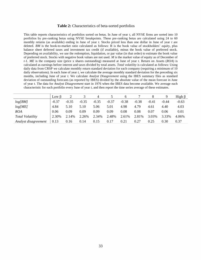
33

Table 2: Characteristics of beta-sorted portfolios

This table reports characteristics of portfolios sorted on betas. In June of year t, all NYSE firms are sorted into 10

portfolios by pre-ranking betas using NYSE breakpoints. These pre-ranking betas are calculated using 24 to 60

monthly returns (as available) ending in June of year t. Stocks priced less than one dollar in June of year t are

deleted. BM is the book-to-market ratio calculated as follows: B is the book value of stockholders’ equity, plus

balance sheet deferred taxes and investment tax credit (if available), minus the book value of preferred stock.

Depending on availability, we use the redemption, liquidation, or par value (in that order) to estimate the book value

of preferred stock. Stocks with negative book values are not used. M is the market value of equity as of December of

t-1. ME is the company size (price x shares outstanding) measured at June of year t. Return on Assets (ROA) is

calculated as earnings before interest and taxes divided by total assets. Total volatility is calculated as follows: Using

daily data from CRSP we calculate monthly return standard deviation for each company (requiring a minimum of 10

daily observations). In each June of year t, we calculate the average monthly standard deviation for the preceding six

months, including June of year t. We calculate Analyst Disagreement using the IBES summary files as standard

deviation of outstanding forecasts (as reported by IBES) divided by the absolute value of the mean forecast in June

of year t. The data for Analyst Disagreement start in 1976 when the IBES data become available. We average each

characteristic for each portfolio every June of year t, and then report the time series average of these estimates.

Low β 2 3 4 5 6 7 8 9 High β

log[BM] -0.37 -0.35 -0.35 -0.35 -0.37 -0.38 -0.38 -0.41 -0.44 -0.63

log[ME[ 4.84 5.10 5.10 5.06 5.01 4.98 4.79 4.61 4.40 4.03

ROA 0.06 0.09 0.09 0.09 0.09 0.08 0.08 0.07 0.06 0.01

Total Volatility 2.30% 2.14% 2.26% 2.34% 2.48% 2.61% 2.81% 3.03% 3.33% 4.06%

Analyst disagreement 0.13 0.16 0.14 0.15 0.17 0.21 0.27 0.25 0.30 0.37

34

Table 3: Descriptive statistics and correlation coefficients

This table reports descriptive statistics (Panel A) and Pearson correlation coefficients (Panel B). Post-formation

betas (Rolling betas) are calculated using the returns of the size-beta sorted portfolios and the CRSP value-

weighted portfolio as a proxy for the market. They are calculated as the sum of the slopes in the regression of

returns on the current and lagged market return. Rolling beta is obtained by performing the regression each

month using five years of past data. The full sample beta [FF beta – as used by Fama and French (1992)] is

calculated by running one regression only for each size-beta portfolio using the data from the entire sample

period. ME is the company size (price x shares outstanding) measured at June of year t. BM is the book-to-

market ratio calculated as follows: B is the book value of stockholders’ equity, plus balance sheet deferred taxes

and investment tax credit (if available), minus the book value of preferred stock. Depending on availability, we

use the redemption, liquidation, or par value (in that order) to estimate the book value of preferred stock. Stocks

with negative book values are not used. M is the market value of equity as of December of t-1. ME is the

company size (price x shares outstanding) measured at June of year t. In the Fama-MacBeth regressions these

variables are matched with CRSP returns for the months of July of year t to June of year t+1. Ret1 is the return

of stock i in month t-1. Ret6 is cumulative return of stock i in the six months prior to month t-1, and Ret12 is the

cumulative return from of stock i in the six months prior to month t-7. Our sample covers the period 1966-2010.

Panel A: Descriptive Statistics

Mean Std. Dev. Median Q1 Q3

Rolling beta 1.31 0.46 1.24 0.98 1.57

FF beta 1.30 0.34 1.24 1.03 1.51

log[ME] 4.80 2.08 4.64 3.28 6.18

log[BM] -0.44 0.90 -0.37 -0.94 0.13

Panel B: Correlation Coefficients

Rolling beta FF beta log[ME] log[BM] Ret1 Ret6 Ret12

Rolling beta 1 0.81 -0.24 -0.05 0.008 0.036 0.04

[<.0001] [<.0001] [<.0001] [<.0001] [<.0001] [<.0001]

FF beta 1 -0.29 -0.07 0.01 0.03 0.05

[<.0001] [<.0001] [<.0001] [<.0001] [<.0001]

log[ME] 1 -0.37 -0.04 -0.04 0.03

[<.0001] [<.0001] [<.0001] [<.0001]

log[BM] 1 0.03 0.08 -0.04

[<.0001] [<.0001] [<.0001]

Ret1 1 -0.02 0.003

[<.0001] [<.0001]

Ret6 1 -0.01

[<.0001]

Ret12 1

35

Table 4: Returns of Beta-Sorted Portfolios

This table reports the average return of beta-sorted portfolios. In June of year t, all firms are sorted into 10 portfolios

by pre-ranking betas using NYSE breakpoints. These pre-ranking betas are calculated using 24 to 60 monthly

returns (as available) ending in June of year t. Stocks priced less than one dollar in June of year t are deleted. We

obtain value-weighted monthly returns for these portfolios from July of year t to June of year t+1, where size is

measured at the end of June of year t. We measure sentiment using the annual index provided by Baker and Wurgler

(2006), orthogonalized with respect to macroeconomic variables. We define all observations in year t as optimistic

(pessimistic) if the sentiment index is positive (negative) in year t-1. We then average portfolio returns and spreads

separately for optimistic and pessimistic months. Our sample covers the period 1966-2010. ** and * denote

significance at the 5% and 10% levels, respectively.

Low β 2 3 4 5 6 7 8 9 High β H-L

All (n=540) 0.90 0.86 0.94 1.04 0.93 1.01 0.89 0.98 1.04 0.89 -0.01

Pess. (n=276) 0.79 0.77 0.87 1.12 1.25 1.12 1.35 1.39 1.67 1.88 1.09**

Opt.(n=264) 1.01 0.95 1.00 0.96 0.59 0.90 0.41 0.55 0.38 -0.15 -1.16**

36

Table 5: Fama-MacBeth regressions

This table reports the average slopes of each variable from the monthly regressions for the period 1966-2010. The t-statistic is the average slope divided by its time series standard

error. We use Newey-West correction on the standard errors to control for heteroscedasticity and autocorrelation. Stocks priced less than one dollar in month t-1 are not included in the

regressions. In Panel A we average the slopes for our entire sample period. In panels B and C we define each month t as pessimistic or optimistic, respectively, and average the slopes

separately for each group. We measure sentiment using the annual index provided by Baker and Wurgler (2006) orthogonalized with respect to macroeconomic variables. We define all

observations in year t as optimistic (pessimistic) if the sentiment index is positive (negative) in year t-1. Stocks are assigned into size-beta portfolios in June of year t and remain in that

classification for 12 months. Stocks are assigned post formation rolling beta (β) in month t, which are obtained from the regression of size-beta portfolio returns on market returns using

five years of data ending in month t-1. ME is the company size (price x shares outstanding) measured at June of year t. BM is the book-to-market ratio calculated as follows: B is the

book value of stockholders’ equity, plus balance sheet deferred taxes and investment tax credit (if available), minus the book value of preferred stock. Depending on availability, we

use the redemption, liquidation, or par value (in that order) to estimate the book value of preferred stock. Stocks with negative book values are not used. M is the market value of equity

as of December of t-1. These variables are matched with CRSP returns for the months of July of year t to June of year t+1. Ret1 is the return of stock i in month t-1. Ret6 is cumulative

return of stock i in the six months prior to month t-1, and Ret12 is the cumulative return from of stock i in the six months prior to month t-7. In Panel A, the average number of

companies in each cross sectional regression is 3,037, 2,894 in Panel B, and 3,186 in Panel C.

Panel A: All (n=540) Panel B: Pessimistic (n=276) Panel C: Optimistic (n=264)

β ln[ME] ln[B/M] Ret1 Ret6 Ret12 β ln[ME] ln[B/M] Ret1 Ret6 Ret12 β ln[ME] ln[B/M] Ret1 Ret6 Ret12

0.31 1.46 -0.88

[1.04] [3.50] [-2.64]

0.04 -0.11 0.97 -0.21 -0.93 -0.02

[0.16] [-3.14] [2.48] [-3.99] [-2.83] [-0.34]

0.18 -0.07 0.28 0.97 -0.17 0.20 -0.65 0.04 0.37

[0.69] [-1.81] [4.26] [2.59] [-3.26] [2.26] [-2.23] [0.86] [4.15]

0.16 -0.07 0.30 -0.05 0.97 -0.17 0.22 -0.06 -0.68 0.04 0.38 -0.04

[0.63] [-1.79] [4.41] [-11.11] [2.54] [-3.13] [2.46] [-8.13] [-2.26] [0.85] [4.17] [-8.03]

0.10 -0.07 0.29 -0.05 0.005 0.84 -0.17 0.21 -0.06 0.001 -0.69 0.03 0.37 -0.04 0.009

[0.40] [-1.95] [4.31] [-11.23] [2.31] [2.42] [-3.24] [2.35] [-8.24] [0.21] [-2.37] [0.69] [4.13] [-8.10] [4.30]

0.11 -0.08 0.30 -0.05 0.004 0.006 0.85 -0.17 0.25 -0.06 0.000 0.005 -0.65 0.02 0.37 -0.04 0.009 0.007

[0.48] [-2.17] [4.76] [-11.53] [2.21] [4.12] [2.53] [-3.37] [2.79] [-8.50] [0.16] [2.04] [-2.31] [0.50] [4.40] [-8.27] [4.15] [4.25]

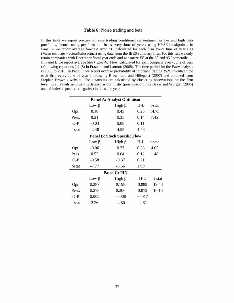
37

Table 6: Noise trading and beta

In this table we report proxies of noise trading conditional on sentiment in low and high beta

portfolios, formed using pre-formation betas every June of year t using NYSE breakpoints. In

Panel A we report average forecast error FE, calculated for each firm every June of year t as

(Mean estimate – actual)/abs(actual) using data from the IBES summary files. For this test we only

retain companies with December fiscal year ends and winsorize FE at the 5th

and 95th

percentile.

In Panel B we report average Stock Specific Flow, calculated for each company every June of year

t following equations (1)-(8) in Frazzini and Lamont (2008). The time period for the Flow analysis

is 1983 to 2010. In Panel C we report average probability of informed trading PIN, calculated for

each firm every June of year t following Brown and and Hillegeist (2007) and obtained from

Stephen Brown’s website. The t-statistics are calculated by clustering observations on the firm

level. In all Panels sentiment is defined as optimistic (pessimistic) if the Baker and Wurgler (2006)

annual index is positive (negative) in the same year.

Panel A: Analyst Optimism

Low β High β H-L t-stat

Opt. 0.18 0.43 0.25 14.73

Pess. 0.21 0.35 0.14 7.42

O-P -0.03 0.08 0.11

t-stat -2.48 4.55 4.46

Panel B: Stock Specific Flow

Low β High β H-L t-stat

Opt. -0.06 0.27 0.33 4.05

Pess. 0.52 0.64 0.12 1.48

O-P -0.58 -0.37 0.21

t-stat -7.77 -5.56 1.90

Panel C: PIN

Low β High β H-L t-stat

Opt. 0.287 0.198 0.089 19.43

Pess. 0.278 0.206 0.072 16.13

O-P 0.009 -0.008 -0.017

t-stat 2.26 -4.80 -2.81

38

Table 7: Small Investor Order Imbalance

The table presents order imbalance (SOIB) for small investors calculated from TAQ data for the low and high beta

portfolios. For this test we use NYSE and AMEX stocks for the period 1980-2010.We follow Hvidkjaer (2006, 2008) to

match trades to quotes, and to identify small and large investor trades. From the daily small investor SOIB for each

company we subtract the market-wide imbalance for small investors on that day. We delete top 1% of daily SOIB

observations according to small trader turnover and large trader turnover (buy volume +sell volume)/market value)). In

Panel A we average daily SOIB for each company and month, and then report the average monthly SOIB for the 6

month period ending in June of year t. In Panel B we calculate earnings surprises using the seasonal random walk

model. We assign a beta classification to each event-firm, and rank all event-firms in a given fiscal period and beta

group in 4 standardized unexpected earnings groups (SUE). In panel B we report average SOIB for the days [-1,0],

where 0 is the earnings announcement date, for SUE groups 1 (negative surprise) and 4 (positive surprise). In Panel C

(D) we follow the same procedure but the event analyzed is analyst recommendations (analyst earnings forecasts),

which we split to upward and downward. In Panel D all revisions that exceed 100% in absolute value are deleted. T-

statistics are calculated by clustering observations on the firm level. In all Panels sentiment is defined as optimistic

(pessimistic) if the Baker and Wurgler (2006) annual index is positive (negative) in the same year.

Panel A: Beta Portfolios

Beta portfolio Opt. Pess. Opt.-Pess. t-stat Opt. Pess. Opt.-Pess. t-stat

1 -0.005 -0.008 0.003 0.33

10 0.009 -0.021 0.030 4.77

10-1 0.014 -0.013 0.027 2.38

t-stat 1.80 -1.58

Panel B : Earnings announcements

B1:SUE=4

B2:SUE=1

1 -0.023 -0.045 0.022 1.09 -0.077 -0.056 -0.021 -1.01

10 0.054 -0.005 0.059 2.51 -0.101 -0.072 -0.029 -1.24

10-1 0.077 0.040 0.037 1.17 -0.024 -0.016 -0.008 -0.26

t-stat 3.39 1.79 -1.06 -0.76

Panel C: Analyst recommendations

C1: Upward

C2: Downward

1 -0.039 -0.032 -0.007 -0.44 -0.070 -0.052 -0.018 -1.20

10 0.017 -0.013 0.030 2.03 -0.032 -0.042 0.010 0.65

10-1 0.056 0.019 0.037 1.61 0.038 0.010 0.028 1.22

t-stat 3.36 1.21 2.10 0.66

Panel D: Analyst earnings forecasts

D1: Upward

D2: Downward

1 -0.047 -0.062 0.015 1.39 -0.019 -0.043 0.024 2.10

10 -0.025 -0.05 0.025 2.46 -0.026 -0.041 0.015 1.47

10-1 0.022 0.012 0.01 0.51 -0.007 0.002 -0.009 -0.57

t-stat 1.63 0.97 -0.64 0.17

39

Table 8: Expanded Fama-MacBeth regressions

This table reports the average slopes of each variable from the monthly Fama-MacBeth regressions for

Models 1 and 2 for the period 2/1976-12/2010 for which disp is available from the IBES summary files. The

t-statistic is the average slope divided by its time series standard error. We use Newey-West correction on the

standard errors to control for heteroscedasticity and autocorrelation. Stocks priced less than one dollar in

month t-1 are not included in the regressions. In Panel A, we average the slopes for our entire sample period.

In Panels B and C, we define each month t as pessimistic or optimistic, respectively, and average the slopes

separately for each group. We measure sentiment using the annual index provided by Baker and Wurgler

(2006) orthogonalized with respect to macroeconomic variables. We define all observations in year t as

optimistic (pessimistic) if the sentiment index is positive (negative) in year t-1. Stocks are assigned into size-

beta portfolios in June of year t and remain in that classification for 12 months. Stocks are assigned post

formation rolling beta (β) in month t, which are obtained from the regression of size-beta portfolio returns on

market returns using five years of data ending in month t-1. ME is the company size (price x shares

outstanding) measured at June of year t. BM is the book-to-market ratio calculated as follows: B is the book

value of stockholders’ equity, plus balance sheet deferred taxes and investment tax credit (if available),

minus the book value of preferred stock. Depending on availability, we use the redemption, liquidation, or

par value (in that order) to estimate the book value of preferred stock. Stocks with negative book values are

not used. M is the market value of equity as of December of t-1. These variables are matched with CRSP

returns for the months of July of year t to June of year t+1. Ret1 is the return of stock i in month t-1. Ret6 is

cumulative return of stock i in the 6 months prior to month t-1, and Ret12 is the cumulative return from of

stock i in the six months prior to month t-7. We calculate analyst disagreement (Disp) using the IBES

summary files. Disp is standard deviation of outstanding forecasts (as reported by IBES) divided by the

absolute value of the mean forecast in June in month t-1. IVOL is idiosyncratic volatility in t-1 calculated as

follows: Using daily data we run a monthly regression for each company of returns on MKT (value-weighted

returns of the market from CRSP), HML (High minus Low) and SMB (Small minis Big) and save the

residuals. IVOL is the monthly sum of the squared residuals for each company. The average number of

firms per month in the regressions below is 1,888.

β ln[ME] ln[B/M] Ret1 Ret6 Ret12 Disp IVOL

Panel A: All (n=419)

Model 1 0.01 -0.09 0.18 -0.04 0.01 0.01

[0.05] [-2.41] [2.28] [-8.66] [2.07] [3.68]

Model 2 0.09 -0.12 0.17 -0.04 0.005 0.006 -0.08 -13.64

[0.36] [-3.44] [2.10] [-8.69] [1.85] [3.40] [-2.07] [-5.69]

Panel B: Pessimistic (n=191)

Model 1 0.81 -0.16 0.11 -0.04 0.00 0.002

[2.32] [-2.84] [1.00] [-6.08] [0.12] [0.83]

Model 2 0.83 -0.16 0.11 -0.04 0.00 0.002 -0.04 -4.82

[2.42] [-3.17] [0.98] [-6.26] [0.20] [0.82] [-0.46] [-1.30]

Panel C: Optimistic (n=228)

Model 1 -0.66 -0.03 0.24 -0.04 0.01 0.01

[-2.03] [-0.72] [2.26] [-6.26] [3.27] [4.99]

Model 2 -0.53 -0.09 0.21 -0.04 0.008 0.01 -0.12 -21.03

[-1.68] [-1.83] [2.02] [-6.10] [2.83] [4.47] [-4.05] [-7.63]

40

Table 9: Augmented Sentiment Index

In this table we use the monthly Baker and Wurgler (2007) sentiment index in month t, and the average Stock

Specific Flow, FE and SOIB for high beta in the same month (defined as in Tables 6 and 7, respectively), perform

principal component analysis, and retain the first principal component as an augmented sentiment index. To define

sentiment in month t we average the augmented sentiment index from t-1 to t-7 and define sentiment as optimistic

(pessimistic) if this average is positive (negative). Using this index in Panel A we repeat the analysis conducted in

Table 4 and, in Panel B the analysis of Table 5, using the same methodology as in those tables. The time period for

this test is 1984-2010. ** and * denote significance at the 5% and 10% levels, respectively.

Panel A: Returns on beta-sorted portfolios

Low β High β H-L

Pess. (n=212) 0.91 1.97 1.06**

Opt.(n=113) 1.11 -1.16 -2.27**

Panel B: Fama-MacBeth Regressions

β ln[ME] ln[B/M] Ret1 Ret6 Ret12

B1: Pessimistic (n=212)

0.87 -0.04 0.14 -0.03 0.002 0.001

[2.38] [-0.76] [1.29] [-5.47] [0.68] [0.50]

B2: Optimistic (n=113)

-1.27 0.08 0.53 -0.04 0.008 0.01

[-3.04] [-1.34] [5.00] [-6.37] [2.88] [3.69]

41

Table 10: Beta-sorted Portfolios Cut Different Ways

This table reports the average returns of double-sorted portfolios. Following the procedure of Table 4 we form beta portfolios across sentiment periods and

classify them in groups based on institutional ownership, short ratio and analyst coverage. In panel A we calculate institutional ownership as of June of year t

for each stock. We partition our sample in two groups based on institutional ownership (above and below median within each beta portfolio in each June of

year t), and run the analysis separately for each group. The data for institutional ownership are from Thomson Reuters on WRDS. The time period for this test

is 1981-2010. In Panel B we calculate for each stock monthly short ratio as follows: shares held short/shares outstanding, and then average the short ratio for

each company in the 12 months ending in June of year t. We partition our sample in two groups based on short ratio (above and below median within each beta

portfolio in each June of year t), and run the analysis separately for each group. The time period for this test is 1974-2010. Short sale data are from Compustat.

In Panel C we calculate residual analyst coverage as follows: Each month t we run a cross sectional regression of Log(1+number of analysts)= a +

b*log(Market Value) + e, where number of analysts is provided by the IBES summary files and MV is end of previous year end market value. The residual

from this regression is our measure of analyst coverage in June of year t. We partition our sample in two groups based on residual analyst coverage (above and

below median within each beta portfolio in each June of year t), and run the analysis separately for each group. The time period for this test is 1980-2010. In

all Panels we obtain value-weighted monthly returns for these portfolios from July of year t to June of year t+1, where size is measured at the end of June of

year t. ** and * denote significance at the 5% and 10% levels, respectively.

Low β 2 3 4 5 6 7 8 9 High β H-L

Panel A1:Low Institutional Ownership

Optimistic (n=210) 1.01 0.95 1.32 1.23 0.79 0.77 0.57 0.33 0.11 -0.85 -1.86**

Pessimistic (n=144) 1.01 1.14 1.26 1.41 1.22 1.85 1.97 2.43 2.00 2.28 1.27*

Panel A2: High Institutional Ownership

Optimistic (n=210) 1.07 0.94 1.00 1.01 0.57 0.89 0.32 0.52 0.29 -0.23 -1.30**

Pessimistic (n=144) 0.98 0.94 1.32 1.65 1.71 1.45 1.89 1.76 2.31 2.59 1.61**

Panel B1: Low Short Ratio

Optimistic (n=228) 1.07 1.01 0.96 0.92 0.67 0.71 0.70 0.59 0.43 -0.38 -1.45**

Pessimistic (n=210) 0.82 0.90 0.94 0.77 1.29 1.15 1.09 1.39 1.78 2.08 1.26**

Panel B2: High Short Ratio

Optimistic (n=228) 1.19 1.06 1.18 1.04 0.77 1.02 0.50 0.91 0.65 0.45 -0.74

Pessimistic (n=210) 0.98 0.85 1.15 1.59 1.61 1.63 1.78 1.71 2.09 2.40 1.42**

Panel C1: Low Analyst Coverage

Optimistic (n=222) 1.03 0.89 0.99 0.92 0.41 0.95 0.50 0.57 0.36 -0.40 -1.43**

Pessimistic (n=144) 1.02 0.77 1.39 1.66 1.51 1.54 2.04 1.60 2.37 2.50 1.48**

Panel C2: High Analyst Coverage

Optimistic (n=222) 1.07 1.09 1.18 1.13 0.94 0.93 0.62 0.64 0.83 0.14 -0.93

Pessimistic (n=144) 1.01 1.12 1.43 1.56 1.70 1.59 1.87 2.21 2.40 2.73 1.72**

42

Table 11: Controlling for additional variables

This table reports the average slopes of each variable from the monthly Fama-MacBeth regressions for Models 1 and 2 for the

period 2/1976-12/2010 in optimistic and pessimistic sentiment periods. We measure sentiment using the annual index provided

by Baker and Wurgler (2006) orthogonalized with respect to macroeconomic variables. We define all observations in year t as

optimistic (pessimistic) if the sentiment index is positive (negative) in year t-1. The t-statistic is the average slope divided by its

time series standard error. We use Newey-West correction on the standard errors to control for heteroscedasticity and

autocorrelation. Stocks priced less than one dollar in month t-1 are not included in the regressions. We augment model 2 from

Table 8 with the following variables: Age (the log of the number of years between the first date the firm appears in the CRSP

files and month t), EF (external finance defined as change in assets minus change in retained earnings divided by assets), GS

(change in net sales divided by prior year sales), PrD (dummy variable which takes the value of 1 for firms with positive

earnings (income before extraordinary items+ plus deferred taxes minus preferred dividends, as available) and 0 otherwise), and

DivD (dummy variable which takes the value of 1 for firms with positive dividends per share at the ex-date and 0 otherwise.

β ln[ME] ln[B/M] Ret1 Ret6 Ret12 Disp IVOL Age EF GS PrD DivD

Panel A: Pessimistic (n=191)

0.67 -0.13 0.14 -0.04 0.00 0.00 -0.01 -5.41 -0.01 -0.11 0.09 -0.18 -0.37

[2.34] [-2.46] [1.35] [-6.22] [0.19] [0.77] [-0.08] [-1.44] [-0.14] [-0.62] [1.20] [-0.90] [-2.69]

Panel B: Optimistic (n=228)

-0.53 -0.13 0.21 -0.04 0.01 0.01 -0.11 -19.68 0.11 -0.29 0.04 0.18 0.08

[-1.49] [-2.59] [1.67] [-6.04] [3.03] [4.08] [-3.81] [-6.47] [2.49] [-2.69] [1.32] [0.96] [0.61]

43

Table 12: Alternative beta and sentiment specifications

This table reports the average slopes of each variable from the monthly Fama-MacBeth regressions. The t-statistic is the average slope divided by its time series standard error. We

use the Newey-West correction to the standard errors. Stocks priced less than one dollar in month t-1 are not included in the regressions. In the columns labeled “All,” we average the

slopes for our entire sample period. In the columns labeled “Pessimistic and “Optimistic,” we define each month t as pessimistic or optimistic, respectively, and average the slopes

separately for each group. In Panels 1 and 2 we measure sentiment using the Baker and Wurgler (2006) index as in Table 5. In Panel 1 post formation betas are calculated using the

full sample methodology, as in Fama and French (1992). In Panel 2 we calculate post formation betas using the rolling methodology explained in Table 5, but in the regressions

where we estimate both pre and post formation betas we also include contemporaneous aggregate equity fund flows (calculated as per footnote 24) in addition to the market variables.

The time period for this test is June 1998 to December 2010. In Panels 3 and 4 all the variables are defined as in Table 5 except that we measure sentiment differently. In Panel 3 we

use the consumer confidence index published by the University of Michigan orthogonalized with respect to the macroeconomic variables used by Baker and Wurgler (2006). To

define sentiment in month t we average the residuals from t-1 to t-7 and define sentiment as optimistic (pessimistic) if this average is positive (negative). In panel 4 we use the raw

Michigan index which we average from t-1 to t-7. If the rolling average ending at t-1 is above (below) the sample median rolling sentiment the observation in month t is defined as

optimistic (pessimistic). The time period in Panels 3 and 4 is 1978-2010, when the Michigan index is available on a monthly basis. In Panel 5 we use the monthly Baker and Wurgler

sentiment index orthogonalized with respect to macroeconomic variables, which we further orthogonalize with respect to the TED spread, inflation, aggregate disagreement

calculated from analyst earnings forecasts (as in Hong and Sraer (2012), and disagreement about market returns using data from the Survey of Professional Forecasters (as in

Anderson et al 2009). Because the latter measure of disagreement is available on quarterly basis we use linear interpolation to obtain monthly observations. To define sentiment in

month t we average the residuals from t-1 to t-7 and define sentiment as optimistic (pessimistic) if this average is positive (negative). The time period for this test is 1986-2010, for

which LIBOR data are available.

All Pessimistic Optimistic

β ln[ME] ln[B/M] Ret1 Ret6 Ret12 β ln[ME] ln[B/M] Ret1 Ret6 Ret12 β ln[ME] ln[B/M] Ret1 Ret6 Ret12

Panel 1: Full sample betas

n=540

n=276

n=264

0.07 -0.07 0.30 -0.05 0.04 0.006 0.82 -0.15 0.25 -0.06 0.00 0.005 -0.71 0.02 0.36 -0.04 0.009 0.007

[0.29] [-1.89] [4.76] [-11.54] [2.21] [4.32] [2.38] [-2.84] [2.84] [-8.49] [0.15] [2.17] [-2.38] [0.39] [4.35] [-8.30] [4.18] [4.39]

Panel 2: Controlling for fund flows

n=151

n=72

n=79

0.52 -0.06 0.12 -0.02 0.00 0.00 2.10 -0.18 0.04 -0.02 -0.01 -0.01 -0.91 0.05 0.19 -0.01 0.008 0.004

[1.01] [-0.87] [0.89] [-1.77] [-0.07] [-0.59] [3.41] [-2.22] [0.21] [-3.67] [-1.01] [-1.95] [-1.36] [0.46] [1.07] [-0.73] [1.65] [1.83]

44

Table 12: Continued

All Pessimistic Optimistic

β ln[ME] ln[B/M] Ret1 Ret6 Ret12 β ln[ME] ln[B/M] Ret1 Ret6 Ret12 β ln[ME] ln[B/M] Ret1 Ret6 Ret12

Panel 3: Michigan consumer confidence index┴

n=391

n=165

n=220

0.12 -0.03 0.27 -0.04 0.005 0.005 0.85 -0.10 0.19 -0.04 0.001 0.003 -0.4 0.02 0.33 -0.03 0.008 0.006

[0.43] [-0.81] [3.72] [-9.59] [2.26] [3.52] [2.19] [-1.90] [1.76] [-7.00] [0.16] [1.16] [-1.11] [0.41] [3.42] [-6.95] [4.83] [4.46]

Panel 4: Michigan consumer confidence index

n=391

n=195

n=196

0.12 -0.03 0.27 -0.04 0.005 0.005 0.81 -0.09 0.21 -0.04 0.001 0.003 -0.56 0.03 0.34 -0.03 0.009 0.006

[0.43] [-0.81] [3.72] [-9.59] [2.26] [3.52] [2.10] [-1.80] [2.16] [-7.07] [0.21] [1.54] [-1.47] [0.53] [3.15] [-6.72] [5.14] [4.14]

Panel 5: Controlling for Inflation, Leverage Constraints and Disagreement

n=295

n=181

n=114

0.24 -0.01 0.25 -0.03 0.003 0.003 1.17 -0.06 0.06 -0.02 0.002 0.002 -1.10 0.06 0.52 -0.04 0.005 0.005

[0.72] [-0.24] [2.87] [-7.20] [1.19] [1.73] [2.56] [-0.97] [0.52] [-4.20] [0.42] [0.72] [-2.71] [1.04] [5.08] [-6.18] [2.43] [2.44]

45

Table 13: Controls for Market Returns

This table reports the average return of beta-sorted portfolios. In June of year t, all firms

are sorted into 10 portfolios by pre-ranking betas using NYSE breakpoints. These pre-

ranking betas are calculated using 24 to 60 monthly returns (as available) ending in June of

year t. Stocks priced less than one dollar in June of year t are deleted. We obtain value-

weighted monthly returns for these portfolios from July of year t to June of year t+1,

where size is measured at the end of June of year t. In Panel A we regress the spread

between the high and the low beta portfolio at time t on a constant and the excess market

return at time t separately in optimistic and pessimistic sentiment periods. In Panel B we

run a Fama-MacBeth cross sectional regression of returns on a constant and beta (defined

as in Table 5) interacted with market returns and report the time series averages of these

parameters. We measure sentiment using the annual index provided by Baker and Wurgler

(2006), orthogonalized with respect to macroeconomic variables. We define all

observations in year t as optimistic (pessimistic) if the sentiment index is positive

(negative) in year t-1. In both Panels the t-statistics are calculated by correcting for

autocorrelation and heteroscedasticity using the Newey-West (1987) estimator.

Panel A: Time series Panel B: Fama-MacBeth

Parameter Estimate t-stat Parameter Estimate t-stat

Pessimistic Pessimistic

a 0.004 1.15 a -0.08 -0.24

b 0.96 8.03 b 0.78 1.87

Optimistic Optimistic

a -0.01 -4.50 a 1.74 6.05

b 1.03 11.63 b 3.26 1.03

46

Figure 1: Beta, sentiment and returns

This figure depicts the relationships between beta and returns. The x-axis shows portfolio average returns and the y-

axis average portfolio beta. To obtain beta portfolios in June of year t, all firms are sorted into 20 portfolios by pre-

ranking betas using NYSE breakpoints. These pre-ranking betas are calculated using 24 to 60 monthly returns (as

available) ending in June of year t. Stocks priced less than one dollar in June of year t are deleted. We obtain value-

weighted monthly returns for these portfolios from July of year t to June of year t+1, where size is measured at the

end of June of year t. We measure sentiment using the annual index provided by Baker and Wurgler (2006)

orthogonalized with respect to macroeconomic variables. We define all observations in year t as optimistic

(pessimistic) if the sentiment index is positive (negative) in year t-1. We then average portfolio returns separately for

optimistic and pessimistic months. The left panel shows the relationship between beta and returns for the entire

sample period and the right Panel only in pessimistic sentiment periods.