WP-2018-008

Investment Choice with Managerial Incentive Schemes

Shubhro Sarkar and Suchismita Tarafdar

Indira Gandhi Institute of Development Research, MumbaiMarch 2018

Investment Choice with Managerial Incentive Schemes

Shubhro Sarkar and Suchismita Tarafdar

Email(corresponding author): suchismita.tarafdar@snu.edu.in

AbstractIn this paper we show that firms might get an additional strategic benefit from using

marginal-cost-reducing investments in conjunction with a managerial incentive scheme. While both

these instruments allow firms to \aggressively" participate in product market competition, we show that

they act as strategic substitutes or complements depending on whether they are chosen simultaneously

or sequentially under complete information. Given that the use of such instruments is inseparably linked

with a Prisoner's Dilemma kind of situation, our analysis shows a way to mitigate such effects, through

their simultaneous use.

Keywords: Strategic delegation, Cost-Reducing Investment, Strategic Substitutes, StrategicComplements, Subgame Perfection.

JEL Code: C72, L13, D43.

Investment Choice with Managerial IncentiveSchemes

Shubhro Sarkar∗ Suchismita Tarafdar†

December 21, 2017

Abstract

In this paper we show that firms might get an additional strategicbenefit from using marginal-cost-reducing investments in conjunctionwith a managerial incentive scheme. While both these instrumentsallow firms to “aggressively”participate in product market competi-tion, we show that they act as strategic substitutes or complementsdepending on whether they are chosen simultaneously or sequentiallyunder complete information. Given that the use of such instrumentsis inseparably linked with a Prisoner’s Dilemma kind of situation, ouranalysis shows a way to mitigate such effects, through their simulta-neous use.

∗Indira Gandhi Institute of Development Research.†Corresponding author: Department of Economics, Shiv Nadar University. Email:

suchismita.tarafdar@snu.edu.in

1

1 Introduction

In the strategic delegation literature there are several studies which showthat the R&D incentives of managerial firms are different from those of en-trepreneurial ones. However, these models consider direct strategic effects ofinvestments only. We show, inter alia, that investments made by firms couldhave an (additional) indirect strategic benefit, which has so far, not beenstudied. To avail of such benefits, the owners of these firms need to use anadditional instrument, which is known to fetch a strategic advantage. Weuse managerial incentives as the second instrument, which has been shownto lead to stronger (weaker) product market competition if the goods arestrategic substitutes (complements) (Fershtman and Judd (FJ, 1987))1.

Since investment choices made by a firm serve multiple purposes, weassume that such decisions are made by the owners rather than by theiragents. Our assumption is backed by a general perception in the literaturethat though business-unit managers take day-to-day tactical decisions, majordecisions such as capacity increases, major capital investments, performanceappraisal and selection of managerial incentive schemes are taken by ownersand directors (Sengul et. al. (2012), Collis and Montgomery (2005), Holm-strom and Costa (1986)). Using a quantity competition model with demanduncertainty, we then pose the following research questions:

1. is the level of investment higher or lower in a setup in which two in-struments are used rather than one?

2. does the answer to the above question depend of the timing of thesechoices?

3. how does the choice of the managerial incentive scheme vary as thelevel of investment changes?

4. what is the optimal sequencing of these instruments from the perspec-tive of the owners?

5. does the answer to the above question change when the focus shifts towelfare maximization?

1The use of such a second instrument is in fact a dominant strategy for the incumbentfirms.

2

Given that both these instruments are known to effectuate stronger productmarket competition in a quantity-competition setting, it is not immediatelyobvious whether they would behave as complements or substitutes.

Our paper follows the literature which shows that firms use a variety ofmeans to compete more aggressively in the product market. These strate-gies are referred to as “top-dog strategies”by Fudenberg and Tirole (1984)and include inter alia, R&D (Brander and Spencer (1983)), debt obligation(Brander and Lewis (1986)), sticky prices (Fershtman and Kamien (1987)),franchise systems (Esther Gal-Or (1995)) and capacity constraints (Spence(1977, 1979) and Dixit (1980)). However, as all players attempt to push theiropponents into a less aggressive position, it results in a situation similar toa Prisoner’s Dilemma in which, equilibrium payoffs are Pareto-dominated byan outcome in which such strategies are not used.

The genesis of the literature on strategic delegation is credited to FJ(1987), Sklivas (1987) and Vickers (1985). (footnote: For an exhaustivereview of the literature on strategic delegation, please refer to Sengul et.al. (2012)). Vickers (1985) and FJ (1987) show how oligopolistic ownerscan increase profits by offering managers an incentive scheme which is basedon profits as well as sales. In the case of Bertrand-price competition withdifferentiated products, FJ (1987) shows that owners incentivize managers toset high prices. They do so by overcompensating the agents and set negativeweights on sales. The literature on investments made to reduce marginalcosts is older and shows that these investments allow firms to compete morevigorously and leads rivals either to compete less vigorously or to exit theindustry altogether (Spence (1979), Dixit (1980), Eaton and Lipsey (1981)).Papers which focus on the strategic incentives of investment build on theseminar work of Fudenberg and Tirole (1984) and Bulow et. al. (1985). Theyargue that players make their long-term decisions while considering theirimpact on the investment decisions of their rivals. Depending on whethersuch investments are “soft”or “aggressive”and the nature of product marketcompetition, firms invest more or less than they would have in the absenceof such strategic effects.

We are not the first to analyze a setup in which firms use two instruments.Clayton (2009) for instance, studies a model in which firms use both leverageand investment in a quantity competition game, and shows that debt withlimited liability lowers the incentive to invest. To construct our argument, wefirst solve an extensive form game in which two owners simultaneously chooseinvestments in the first period and compete in quantities, in the second. We

3

show that the investments made in this setting have two components, onepart which reduces costs and another which provides a strategic benefit.We then show that the equilibrium collapses once firms have the option tostrategically delegate the output decision to a manager (in an interveningperiod). This leads to a setup in which the duopolists choose investmentsand managerial incentives.

We first consider the setup where investment and managerial incentivesare chosen sequentially. In this case, each firm’s owner is aware of the invest-ment level of both the firms when she decides the managerial incentive. Thisleads to an added strategic advantage of signalling to be tough by choosinga higher level of investment, as it reduces (increases) the weight assigned tosales by the rival firm (itself) in the second period. The investment made inthe first period therefore has an (additional) effect on the managerial incen-tives chosen in period 2, which in turn affect output in the last period. Thisis apart from the direct impact of investment on the corresponding outputs.Thus, in the three-stage game, there is an additional strategic advantagewhich is brought in through such sequential play.

In an alternative setting, the investment choices made by the firms in thefirst period are not made public in the second. This essentially reduces thegame into one with two-periods. In the first period incentives and investmentare simultaneously chosen by the owner and output decisions are made bythe manager in the second. Since investment choices are no longer “visible”tothe players when they choose managerial incentives, the former can no longerbe indirectly used to push an opponent into a disadvantageous position. Forthis reason, investment in the simultaneous setup is lower than that in thesequential one. The workings of our model are therefore different from thatof previous studies2 as it allows the investment choices made by the ownerto indirectly impact product market competition through the managerial in-centive scheme. This mechanism was hitherto unavailable in prior studies asinvestment choices were made after the selection of the managerial incentivescheme.

We find that investment in the sequential choice setting is higher thanthat of the benchmark model (I0), it is lower than I0 in the simultaneouscase (Propositions 1 and 2). Hence it is not the case that managerial firmsunambiguously invest more (or less) than their entrepreneurial counterparts.

2See Zhang and Zhang (1997), Kopel and Reigler (2006, 2008), and Mitrokostas andPetrakis (2014).

4

Following this result we show that while the weights assigned to sales in eitherthe simultaneous or sequential setup is higher than that of the FJ model, theowner stresses sales to a larger extent in the sequential case (Proposition 3).The instruments therefore, act as substitutes when they are chosen togetherbut are complements in the sequential setup. Our results indicate that netprofits earned when the instruments are chosen simultaneously dominatethose when they are decided sequentially (Proposition 4). Hence, it is inthe interest of both firms not to divulge their investment decisions to theirrivals. This result is however reversed when we compare welfare across thetwo scenarios (Proposition 7).

2 The Model

We assume that there are two firms, each of which has two players: an owner,who maximizes the firm’s profit, and a manager, who executes the decisionof the owner and makes the output decision. We consider two settings, inone of which the instruments are chosen sequentially, and in the other one,simultaneously. In the sequential setup, the owners simultaneously choose aninvestment level to reduce marginal cost of production in the first period. Inthe second period they simultaneously choose a managerial incentive schemesuch that the individual rationality constraint of the manager is satisfied. Theinvestment levels chosen in the first period, therefore, affect the choices ofmanagerial incentives. In the simultaneous setup, investment and managerialincentives are chosen at the same time in period one. Finally, in the third(second) period the managers choose quantities a la Cournot in the sequential(simultaneous) choice model.

We assume both the managers are risk neutral. We restrict ourselves withthe linear incentive structure as in Fershtman and Judd [8]. The incentivestructure is a linear combination of the profit (gross profit) and total revenuegiven by

Oi = (1− αi)Πi + αiTRi

where 0 ≤ αi < 1. The manager’s remuneration is given by

Ai +BiOi

The constants Ai ≥ 0, Bi > 0 are chosen such that in equilibrium the manager

5

get’s at least her outside option, W i in expectation,

Ai +Bi

∫a

Oif(a)d(a) ≥ W i.

Since Bi is strictly positive, the risk neutral manager seeks to maximize Oi.Emphasizing partly on total revenue is fairly standard, as firms do writecontract with employees to maximize sales (also perhaps the bonus is givenas a function of sales and profit). Other incentive contracts can be writtenbut this is a tractable form to influence output in period 3, to maximizeprofit. The focus of this paper is to show that investment levels change whenoptimal output of the third stage can be influenced by other instruments.Therefore, we assume a tractable incentive structure.

The firms face a linear inverse demand function given by

a− b(qi + qj).

The intercept a, is a random variable with distribution function F (.) overthe range [β, β]. For our purpose, we will be interested in the expectedvalue of a, denoted by a. The uncertainty in demand is resolved before thethird period, following which rival managers choose their corresponding levelsof output. Thus, one justification for having managers can be that ownersmaximize profit but do not get involved in the day to day working of the firm.The manager takes into account the actual demand realized and chooses theoptimal quantities. In the absence of uncertainty, the owners can write acontract explicitly stating the quantity to be chosen to the managers. Thiswould take away the strategic advantage, as the rival manager’s choice wouldno longer be a function of the third period quantity, i.e., each manager’schoice would have no effect on the choice of the other.

In this case, each firm has two types of fixed costs and one variable cost.The fixed costs are wages paid to the manager and investments made toreduce the marginal cost, while the variable cost component is representedby the marginal cost, c(I). We maintain the following basic assumptions.Assumption 1: The marginal cost c(I), is a mapping c : IR+ → IR++ andsatisfies c′ < 0, c′′ > 0. Further, we assume that β > c(0).Assumption 2: We define µ : IR+ → IR as µ(I) = (a− c(Ii)) c′(Ii), andassume µ(I) is an increasing function.Assumption 1 ensures that in all states, the variable profit for both firms ispositive, while assumption 2 ensures that the necessary second order condi-

6

tions hold while solving for the optimal investment with or without manage-rial incentives.

Using these assumptions we solve for the subgame perfect Nash equilibrium(SPNE). We proceed to the third stage and compute the Nash equilibriumgiven the investment levels, the managerial incentives of both firms, and therealized demand. The manager maximizes her incentive as follows:

maxqi

V i = maxqi

(a− b(qi + qj)− (1− αi)c(Ii))qi

The first order condition is given as:

V ii = a− 2bq∗i − bqj − (1− αi)c(Ii) = 0

The second order condition holds as

V iii = −2b < 0; V i

ij = −b < 0

Since, V iii < V i

ij < 0 the best response functions are downward slopping,with slope greater than −1, for both i, j = 1, 2. as in a standard model.

The optimal quantity for i, j = 1, 2, i 6= j, is given by,

q∗i =a− 2(1− αi)c(Ii) + (1− αj)c(Ij)

3b.

Any increase in own managerial incentives and investment affects the optimalquantity choices of the third stage. Both these have similar effect on the thirdperiod, reducing the effective marginal cost for the manager. Lower effectivemarginal cost translates to an aggressive behavior of the firm, which in turnwould reduce the equilibrium quantity of the rival firm since best responsesare downward slopping. Thus we get the following comparative static formanagerial incentives and investment levels.

∂q∗i∂αi

=2c(Ii)

3b;∂q∗i∂αj

= −c(Ij)3b

∂q∗i∂Ii

= −2(1− αi)c′(Ii)3b

> 0;∂q∗i∂Ij

=(1− αj)c′(Ij)

3b< 0.

For any increase in investment level or managerial incentives, the increasein own output outweighs the decrease in rival’s output, since, the best re-sponse functions are downward slopping with slope greater than −1. There-fore the total output increases with any increase in managerial incentives orinvestment levels for either firm. We now analyze the optimal investmentswithout any managerial incentives.

7

2.1 The Benchmark Case: No Managerial Incentives

The benchmark case is the optimal investment under no managerial incen-tives, that is, αi is set to zero. We thus, consider a two period model, withquantity competition in the second stage and investment choice in the firststage. We denote the optimal quantities of the second stage with no man-agerial incentives as q0i , and q0j . The second stage optimization exercise ofthe manager remains the same. Without managerial incentives, wages are afunction of just profits in each state. In the first stage the owner maximizesthe expected profit net of investment and wages paid to the manager.

maxIi

Y i = maxIi

∫(a− b(q0i + q0j )− c(Ii))q0i f(a)da− Ii

−Ai −Bi

∫a

(a− b(q0i + q0j )− c(Ii)q0i )f(a)d(a)i

subject to

Ai +Bi

∫a

(a− b(q0i + q0j )− c(Ii)q0i )f(a)d(a) ≥ W i

with

q0i =a− 2c(Ii) + c(Ij)

3bi, j = 1, 2, i 6= j. From the principle of optimality, the inequality constraintwill be binding. Thus, the objective function simplifies to:

maxIi

Y i = maxIi

{∫(a− b(q0i + q0j )− c(Ii))q0i f(a)da− Ii −W i

}.

The manager is paid exactly her outside option.The first order condition is

Y iIi

= (a− 2bq0i − bq0j − c(Ii))dq0idI i− bq0i

∂q0j∂I i− c′(Ii))q0i − 1 (1)

while the second order condition is given by

Y iIiIi

=8c′(I0i )c′(I0i )

9b− 4(a− 2c(I0i ) + c(Ij))

9bc′′(I0i ) < 0

The optimal investments with no managerial incentives is given by equation1, where the first term is zero from the equilibrium condition of the product

8

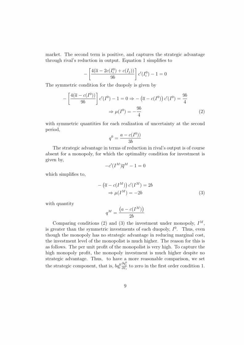
market. The second term is positive, and captures the strategic advantagethrough rival’s reduction in output. Equation 1 simplifies to

−[

4(a− 2c(I0i ) + c(Ij))

9b

]c′(I0i )− 1 = 0

The symmetric condition for the duopoly is given by

−[

4(a− c(I0))9b

]c′(I0)− 1 = 0⇒ −

(a− c(I0)

)c′(I0) =

9b

4

⇒ µ(I0) = −9b

4(2)

with symmetric quantities for each realization of uncertainty at the secondperiod,

q0 =a− c(I0))

3b

The strategic advantage in terms of reduction in rival’s output is of courseabsent for a monopoly, for which the optimality condition for investment isgiven by,

−c′(IM)qM − 1 = 0

which simplifies to,

−(a− c(IM)

)c′(IM) = 2b

⇒ µ(IM) = −2b (3)

with quantity

qM =

(a− c(IM)

)2b

Comparing conditions (2) and (3) the investment under monopoly, IM ,is greater than the symmetric investments of each duopoly, I0. Thus, eventhough the monopoly has no strategic advantage in reducing marginal cost,the investment level of the monopolist is much higher. The reason for this isas follows. The per unit profit of the monopolist is very high. To capture thehigh monopoly profit, the monopoly investment is much higher despite nostrategic advantage. Thus, to have a more reasonable comparison, we set

the strategic component, that is, bq0i∂q0j∂Ii

to zero in the first order condition 1.

9

In the absence of any strategic advantage the symmetric investment level is:

−c′(I)q0 − 1 = 0

⇒ −(a− c(I)

)c′(I) = 3b

⇒ µ(I) = −3b (4)

Comparing (4) with (3) and (2) we find

I < I0 < IM

Thus the symmetric optimal investment can be decomposed into twoparts: an I amount is to increase the profit margin per unit of output. Anyinvestment above this, is for strategic advantage. Now a natural question isif the strategic advantage can be gained through another instrument, wouldthe optimal investment fall to the level of I? In the next section we intro-duce managerial incentives in the intermediary step to capture this strategicadvantage. A discussion on whether the optimal investment made in thebenchmark model is efficient, is included in the appendix. The symmetricequilibrium price and expected gross profits in the benchmark case are,

p0 =a+ 2c(I0)

3; Π0 =

(a− c(I0))2 + σ2

9b−W.

where σ2 denotes the variance of the random variable a.We now show that a firm can do better by strategically delegating the

output decision to a manager using an incentive scheme which is identical tothe one described above. This implies that it will always be in the interestof firm i to deviate and choose an αi > 0, provided such an option opensup in the intervening period. The third-period product market competitiontherefore involves manager of firm i maximizing V i = (a− b(qi + qj)− (1−αi)c(Ii))qi, while the rival manager maximizes Πj = (a− b(qi + qj)− c(Ij))qj.The reaction functions for the two firms are given by

qi =1

3b(a+ c(Ij)− 2(1− αi)c(Ii)); qj =

1

3b(a+ c(Ii)(1− αi)− 2c(Ij)).

The maximization problem for firm i therefore is given by

maxαi

∫(a− b(qi(αi, Ii, Ij) + qj(αi, Ii, Ij))− c(Ii))qi(αi, Ii, Ij)f(a)da

10

The associated first order condition is∫((a− 2bqi(αi, Ii, Ij)− bqj(αi, Ii, Ij)− c(Ii)

dqidαi− bqi(αi, Ii, Ij)

dqjdαi

)f(a)da = 0

=⇒ αi =1

4c(Ii)(a+ c(Ij)− 2c(Ii)).

Since these calculations are done off the equilibrium path, following thechoices made in period 1, we can assume that Ii = Ij such that c(Ii) =

c(Ij). Hence, αi = 14c(Ii)

(a − c(Ii)). Assuming c(Ii) = k −√bI we get

αi = 14c(Ii)

97(a − k) > 0. This is turn implies that the reaction curve for

firm i will lie above the reaction curve for the same firm without such del-egation, while the reaction curve for firm j stays unchanged. This ensuresthat there is an incentive for both firms to use the additional instrument ofstrategic delegation.

2.2 Three-period Model (Sequential Case)

In this section we analyze how the optimal investment level changes in thepresence of managerial incentives. Managerial incentives, like investment,reduces the effective marginal cost in the product competition stage. Wheneffective marginal cost is lowered, the optimal quantity of period three in-creases, thereby reducing rival’s optimal quantity. Reduction in rival outputincreases prices ceteris paribus, which is gainful for the firm. This strategicadvantage of signalling to be aggressive, is identical for both investments andmanagerial incentives. Hence, the owner views these two as instruments toinfluence product market behavior in the same way. However, even thoughthese two instruments affect the product market competition in the sameway, to the owners these two instruments might be strategic complements orsubstitutes depending on whether the instruments are chosen simultaneouslyor sequentially.

We first consider the case where the two instruments are chosen sequen-tially. Thus, before choosing the managerial incentive both the owners knowthe rival’s firm investment level. Consequently, investment has an additionalrole: a higher investment not only signals an aggressive behavior directlyby reducing marginal cost in the product market, but also affects the man-agerial incentives of the second period. As shown next, a higher investmentincreases own managerial incentives while reducing the rival’s. A high in-vestment signifies an aggressive managerial incentive choice, which reduces

11

rival’s managerial incentives as the best responses of managerial incentivesare also negatively slopped.

In the second period given the investment levels, Ii, and Ij, and the rival’sincentive αj, the owner of firm i maximizes gross profit less managerial wagesto choose the optimal incentive scheme. The second period optimizationproblem is given by3:

maxαi

W i = maxαi

{∫ ((a− b(q∗i + q∗j − c(Ii)

)q∗i)f(a)da−W i

}where

q∗i =a− 2(1− αi)c(Ii) + (1− αj)c(Ij)

3b

i, j = 1, 2, i 6= j. The first order condition for i = 1, 2 is given as

W iαi

=

∫ ((a− 2bq∗i − bq∗j − c(Ii))

dqidαi− bqi

∂qj∂αi

)f(a)da = 0 (5)

Simplifying,

a+ 4(1− αi)c(Ii) + (1− αj)c(Ij)− 6c(Ii) = 0

The second order condition is given by W iαiαi

= −4c(Ii) < 0. At α = 0the first term of the expression 5 is zero from the equilibrium condition ofthe third stage. The second term captures the strategic benefit of a highermanagerial incentives and is positive. Consequently since the second ordercondition is satisfied, the optimal investment scheme is positive. Particularly,the optimal incentive is given by

α∗i =a− 3c(Ii) + 2c(Ij)

5c(Ii)

The comparative statics of the optimal managerial incentives with respect toown and rival investment is given by:

dαidI i

=− (a+ 2c(Ij)) c

′(Ii)

5c(Ii)c(Ii)> 0,

dαidIj

=2c′(Ij)

5c(Ii)< 0.

3Like in the benchmark case, the expected managerial wages are set at the outsideoption of the manager.

12

Since a − 2c(Ii) > 0, the own effect dominates the cross effect for any real-ization of rival’s investment.

Now in the first period the owners choose the optimal level of investmentto maximize net profit:

maxIi

Y i = maxIi

∫ ((a− b(q∗i + q∗j )− c(Ii))q∗i − Ii

)f(a)da

where

q∗i =a− 2(1− α∗i )c(Ii) + (1− α∗j )c(Ij)

3b

α∗i =a− 3c(Ii) + 2c(Ij)

5c(Ii)

given investments Ii, and Ij, i 6= j. The first order condition is

Y iIi

=

[dq∗idαi

dα∗idI i

+dq∗idαj

dα∗jdI i

+dq∗idI i

] ∫ (a− 2bq∗i − bq∗j − c(Ii)

)f(a)da(a)

−[dq∗jdαi

dα∗idI i

+dq∗jdαj

dα∗jdI i

+dq∗jdI i

] ∫bq∗i f(a)da(a)− c′(Ii)

∫q∗i f(a)da(a)− 1 = 0

⇒ −α∗i c(Ii)[dq∗idαi

dα∗idI i

+dq∗idαj

dα∗jdI i

+dq∗idI i

]−[dq∗jdαi

dα∗idI i

+dq∗jdαj

dα∗jdI i

+dq∗jdI i

] ∫bq∗i f(a)da(a)

−c′(Ii)∫q∗i f(a)da(a)− 1 = 0

Further simplifying from the equilibrium conditions of the first two stages,the first order condition collapses to,

Y iIi

=

[−αic(Ii)

dq∗idαj−∫bq∗i f(a)da(a)

dq∗jdαj

]dα∗jdI i−c′(Ii)

∫q∗i f(a)da(a)−1 = 0

(6)which gives us

Y iIi

= − 12

25b

[a− 3c(I∗i ) + 2c(I∗j )

]c′(I∗i )− 1.

The second order condition is given by

Y iIiIi

=36

25bc′(I∗i )c′(I∗i )− 12

25b

(a− 3c(I∗i ) + 2c(I∗j )

)c′′(I∗i ).

13

In the sequential setup, the investment made by firm i, Ii has an addi-tional effect on αi,αj, which in turn affects qi, qj. This is apart from thedirect impact of the investment Ii on qi, qj. The indirect strategic impact iscaptured by the first term in equation (6), which shows that Ii first reducesαj, which then leads to an increase in own output, qi. The direct strategicbenefit captured through aggressive behavior of the manager leading to areduction in rival’s quantity is captured by

dq∗idI i

∫ (a− 2bq∗i − bq∗j − c(Ii)

)f(a)da(a)−

dq∗jdI i

∫bq∗i f(a)da(a)

−c′(Ii)∫q∗i f(a)da(a)− 1 = 0

which is similar to equation (1) of the benchmark model. The crucial partof the indirect effect is that firms can use investment made in period 1 tosignal to it’s rivals that it is a strong type. In the next proposition we showthat the optimal investment in the sequential setting, I∗, will be higher thanin the benchmark case.

Proposition 1 When managerial incentives and investments are chosen se-quentially, under assumptions 1 and 2, the symmetric optimal investment,I∗ > I0.

Proof. With I∗1 = I∗2 = I∗, the symmetric managerial incentives and quan-tities of second and third period is given by

α∗ =a− c(I)

5c(I); q∗ =

2(a− c(Ii))5b

Thus, the optimal investment satisfies,

− (a− c(I∗)) c′(I∗) =25b

12

⇒ µ(I∗) = −25b

12(7)

Comparing with (2), (3) and (4), it follows that, I < I0 < I∗ < IM .Therefore, investment and managerial incentives act as strategic comple-

ments when investment can influence the rival’s managerial incentive choice.

14

The market price for each state a, and symmetric expected gross and netprofits are

p∗ =a+ 4c(I∗)

5, Π∗ =

2[(a− c(I∗))2 + σ2

]25b

−W,

Π∗N =2[(a− c(I∗))2 + σ2

]25b

−W − I∗.

2.3 Two-period Model (Simultaneous Case)

Next, we consider the case where the owners choose the managerial incen-tives and investment levels simultaneously. Since both the instruments havesimilar effects on the product market competition, the two are strategic sub-stitutes. The first period problem is

maxIi,αi

Y i = maxIi,αi

∫ ((a− b(q∗∗i + q∗∗j )− c(Ii))q∗∗i − Ii

)f(a)da

where ex-post realization of the random variable,

q∗∗i =a− 2(1− α∗∗i )c(Ii) + (1− α∗∗j )c(Ij)

3b.

The first order conditions are

Y iIi

=dq∗∗idI i

∫ (a− 2bq∗∗i − bq∗∗j − c(Ii)

)f(a)d(a)−

dq∗∗jdI i

∫bq∗∗i f(a)d(a)

− c′(Ii)∫q∗∗i f(a)d(a)− 1 = 0

Y iαi

=dq∗∗idαi

∫ (a− 2bq∗∗i − bq∗∗j − c(Ii)

)f(a)d(a)−

dq∗∗jdαi

∫bq∗∗i f(a)d(a) = 0

Further simplifying the first order conditions we get

Y iIi

= (1− αi)c′(Ii)∫ ((

a− 2bq∗∗i − bq∗∗j − c(Ii)) 2

3b− bq∗∗i

1

b

)f(a)d(a)

−c′(Ii)∫q∗∗i f(a)d(a)− 1 = 0 (8)

Y iαi

= c(Ii)

∫ ((a− 2bq∗∗i − bq∗∗j − c(Ii)

) 2

3b− bq∗∗i

1

b

)f(a)d(a) = 0 (9)

15

Since (1 − αi)c′(Ii), c(Ii) > 0, at α∗i , i = 1, 2, the first order condition (8)collapses to,

Y iIi

= c′(I∗∗i )

∫q∗∗i f(a)d(a)− 1 = 0

Since, the optimal managerial incentives are

α∗∗i =a− 3c(Ii) + 2c(Ij)

5c(Ii)

consequently for each realization of a,

q∗∗i =2(a− 3c(Ii) + 2c(Ij))

5b

the first order condition further simplifies to

Y iIi

=2(a− 3c(I∗∗i ) + 2c(I∗∗j ))

5bc′(I∗∗i )− 1 = 0

In this case, the firm benefits from investment through a lower marginal costonly. However, the investment doesn’t fall to the benchmark case withoutstrategic advantage (I), but is lower than the investment without managerialincentives.

Proposition 2 Under assumptions 1 and 2, I < I∗∗ < I0.

Proof. With I∗∗1 = I∗∗2 = I∗∗, the symmetric managerial incentives andquantities of second and third period is given by

α∗∗ =a− c(I∗∗)

5c(I∗∗); q∗∗ =

2(a− c(I∗∗))5b

Thus, the optimal investment satisfies,

− (a− c(I∗∗)) c′(I∗∗) =5b

2

⇒ µ(I∗∗) = −5b

2(10)

Comparing (10) with (2), (3) and (4), we get, I < I∗∗ < I0 < IM .We now compare optimal investment levels in the simultaneous and se-

quential settings.

16

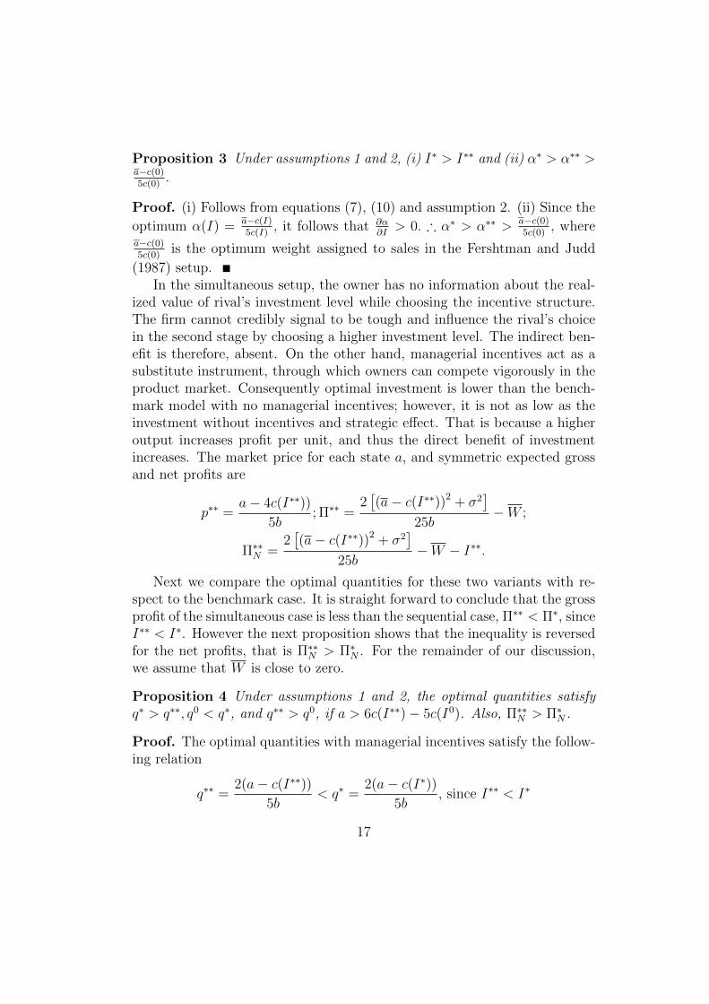
Proposition 3 Under assumptions 1 and 2, (i) I∗ > I∗∗ and (ii) α∗ > α∗∗ >a−c(0)5c(0)

.

Proof. (i) Follows from equations (7), (10) and assumption 2. (ii) Since the

optimum α(I) = a−c(I)5c(I)

, it follows that ∂α∂I> 0. ∴ α∗ > α∗∗ > a−c(0)

5c(0), where

a−c(0)5c(0)

is the optimum weight assigned to sales in the Fershtman and Judd

(1987) setup.In the simultaneous setup, the owner has no information about the real-

ized value of rival’s investment level while choosing the incentive structure.The firm cannot credibly signal to be tough and influence the rival’s choicein the second stage by choosing a higher investment level. The indirect ben-efit is therefore, absent. On the other hand, managerial incentives act as asubstitute instrument, through which owners can compete vigorously in theproduct market. Consequently optimal investment is lower than the bench-mark model with no managerial incentives; however, it is not as low as theinvestment without incentives and strategic effect. That is because a higheroutput increases profit per unit, and thus the direct benefit of investmentincreases. The market price for each state a, and symmetric expected grossand net profits are

p∗∗ =a− 4c(I∗∗))

5b; Π∗∗ =

2[(a− c(I∗∗))2 + σ2

]25b

−W ;

Π∗∗N =2[(a− c(I∗∗))2 + σ2

]25b

−W − I∗∗.

Next we compare the optimal quantities for these two variants with re-spect to the benchmark case. It is straight forward to conclude that the grossprofit of the simultaneous case is less than the sequential case, Π∗∗ < Π∗, sinceI∗∗ < I∗. However the next proposition shows that the inequality is reversedfor the net profits, that is Π∗∗N > Π∗N . For the remainder of our discussion,we assume that W is close to zero.

Proposition 4 Under assumptions 1 and 2, the optimal quantities satisfyq∗ > q∗∗, q0 < q∗, and q∗∗ > q0, if a > 6c(I∗∗)− 5c(I0). Also, Π∗∗N > Π∗N .

Proof. The optimal quantities with managerial incentives satisfy the follow-ing relation

q∗∗ =2(a− c(I∗∗))

5b< q∗ =

2(a− c(I∗))5b

, since I∗∗ < I∗

17

The optimal quantity without managerial incentives, q0 < q∗. To compareq0 with q∗∗, if a > 6c(I∗∗)− 5c(I0) then

q0 =(a− c(I0))

3b< q∗∗ =

2(a− c(I∗∗))5b

.

For the second part, we define a function g : IR+ → IR as

g(I) =2 (a− c(I))2

25b− I

where

g′(I) = −4 (a− c(I)) c′(I)

25b− 1 = 0⇒ µ(I) = −25b

4Since µ is an increasing function, it follows that g achieves a unique maximaat

µ(Imax) = −25b

4.

Using assumption 2 we get Imax < I∗∗ < I∗, implying g′(I) is decreasing inthe range (Imax, I∗], which gives us the result.

Thus, when the owners of each firm have full information of the rival’sinvestment before choosing the managerial incentive structure, their profitfalls. Consequently, both owners would choose not to divulge or seek infor-mation about the other’s investment levels. The following proposition ranksthe expected net profit from the sequential setup with the one earned fromthe benchmark model.

Proposition 5 Under assumptions 1 and 2, Π0N(I0) > Π∗N(I∗).

Proof. Expected net profit in the benchmark model is given by

ΠON =

(a− c(I0))2 + σ2

9b− I0

The expected net profit of the simultaneous or sequential model is given by

ΠN =2(a− c(I))2 + 2σ2

25b− I, where I = I∗, I∗∗.

Since σ2

9b> 2σ2

25bit is enough to show that Π0(I0) = (a−c(I0))2

9b−I0 > 2(a−c(I∗))2

25b−

I∗ = Π(I∗). Since both expressions are functions of I, we write

Π0(I)− Π(I) = (a− c(I))2(1

9b− 2

25b) > 0.

18

Therefore for each value of I, Π0 lies above Π. We now check for the optimuminvestment which maximizes Π0(I0), IB

dΠ0

dI= − 2

9b(a− c(I))c′(I)− 1 = 0

which gives us the first order condition

−(a− c(I))c′(I) =9b

2. (11)

The second order condition is given by

d2Π0

dI2=

2

9b

[(c′(I))2 − (a− c(I))c′′(I)

]< 0

which follows from assumption 2. Similarly the optimum investment levelwhich maximizes Π(I), I is determined from the following first order condi-tion

−(a− c(I))c′(I) =25b

4(12)

Comparing equations (2), (7), (10), (11) and (12), we can show that I∗ >

I0 > I∗∗ > IB > I. Also, since Π(I0) and Π(I) are strictly concave, Π′(I0) <

0 and Π′(I∗), Π′(I∗∗) < 0.

Now assume that Π0(I0) < Π(I∗) < Π(I∗∗). Since I∗ > I0 > I∗∗ we have

Π(I∗) < Π0(I0) < Π(I∗∗), which combined with Π0(I0) < Π(I∗) gives us

Π(I0) > Π0(I0), a contradiction. Hence Π0(I0) > Π(I∗).

In order to compare the expected net profit from the simultaneous setting(Π∗∗N ) with Π0

N , we derive the following sufficient condition.

Proposition 6 Π0N > Π∗∗N if 9b

16(c′(I0))2− I0 > b

2(c′(I∗∗))2− I∗∗.

Proof. Since σ2

9b> 2σ2

25bit is enough to show that Π0

N > Π∗∗N if

(a− c(I0))2

9b− I0 > 2(a− c(I∗∗))2

25b− I∗∗

Using equations (2) and (10) we can show that the above condition simplifiesto 9b

16(c′(I0))2− I0 > b

2(c′(I∗∗))2− I∗∗.

While the expected net profit from the simultaneous setup is higher than thatfrom the sequential setup, we now show that the (ex-ante) social welfare fromthe former (TW ∗) is lower than that of the latter (TW ∗∗).

19

Proposition 7 TW ∗ > TW ∗∗.

Proof. Ex-ante consumer surplus for the sequential case is given as follows

CS∗ =1

2(a− p∗)(q∗1 + q∗2) =

8(a− c(I∗))2

25b.

Total welfare is given by,

TW ∗ = CS∗ + Π∗N =2(a− c(I∗))2 + 2σ2

5b−W − I∗.

Similarly ex-ante total welfare for the simultaneous case is given by

TW ∗∗ =2(a− c(I∗∗))2 + 2σ2

5b−W − I∗∗

The expression

TW (I) =2(a− c(I))2 + 2σ2

5b−W − I

is concave and is maximized at

TW ′(Imax) = −4(a− c(I))c′(Imax)

5b− 1 = 0

Given assumption 2,I∗∗ < I∗ < Imax

which implies that TW ∗∗ < TW ∗.An Example. To illustrate the results obtained so far, we solve the

following example. We use the marginal cost function

c(I) = k −√bI

with k < α which gives us c′(I) = −12

√bI< 0 and c′′(I) = 1

4

√b(I)−3/2 > 0.

Therefore assumption 1 is satisfied. We then assume h(I) = (a−c(I))c′(I) =

(a − k +√bI)(−1

2

√bI). Since h′(I) = (a − k)(1

4

√b(I)−3/2) > 0, therefore,

assumption 2 is satisfied. Using this function, we get

IM =(a− k)2

9b, Io =

4(a− k)2

49b, I =

(a− k)2

25b, I∗ =

36(a− k)2

361b, I∗∗ =

(a− k)2

16b.

20

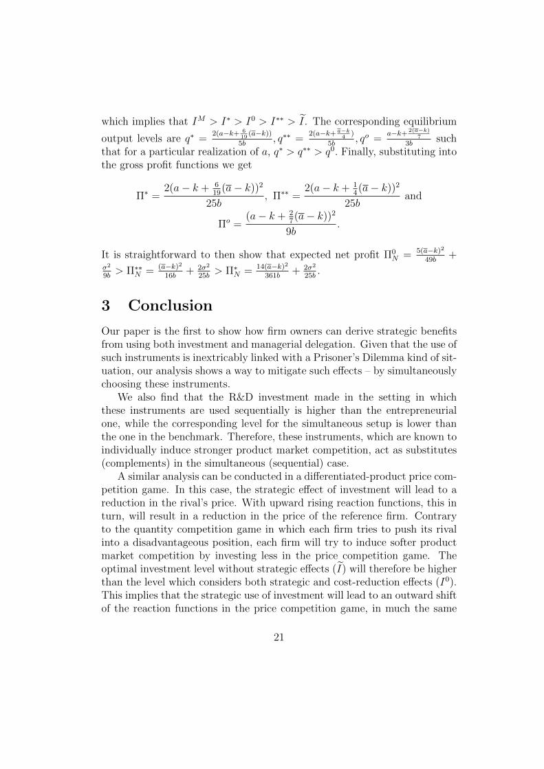
which implies that IM > I∗ > I0 > I∗∗ > I. The corresponding equilibrium

output levels are q∗ =2(a−k+ 6

19(a−k))

5b, q∗∗ =

2(a−k+a−k4

)

5b, qo =

a−k+ 2(a−k)7

3bsuch

that for a particular realization of a, q∗ > q∗∗ > q0. Finally, substituting intothe gross profit functions we get

Π∗ =2(a− k + 6

19(a− k))2

25b, Π∗∗ =

2(a− k + 14(a− k))2

25band

Πo =(a− k + 2

7(a− k))2

9b.

It is straightforward to then show that expected net profit Π0N = 5(a−k)2

49b+

σ2

9b> Π∗∗N = (a−k)2

16b+ 2σ2

25b> Π∗N = 14(a−k)2

361b+ 2σ2

25b.

3 Conclusion

Our paper is the first to show how firm owners can derive strategic benefitsfrom using both investment and managerial delegation. Given that the use ofsuch instruments is inextricably linked with a Prisoner’s Dilemma kind of sit-uation, our analysis shows a way to mitigate such effects – by simultaneouslychoosing these instruments.

We also find that the R&D investment made in the setting in whichthese instruments are used sequentially is higher than the entrepreneurialone, while the corresponding level for the simultaneous setup is lower thanthe one in the benchmark. Therefore, these instruments, which are known toindividually induce stronger product market competition, act as substitutes(complements) in the simultaneous (sequential) case.

A similar analysis can be conducted in a differentiated-product price com-petition game. In this case, the strategic effect of investment will lead to areduction in the rival’s price. With upward rising reaction functions, this inturn, will result in a reduction in the price of the reference firm. Contraryto the quantity competition game in which each firm tries to push its rivalinto a disadvantageous position, each firm will try to induce softer productmarket competition by investing less in the price competition game. Theoptimal investment level without strategic effects (I) will therefore be higherthan the level which considers both strategic and cost-reduction effects (I0).This implies that the strategic use of investment will lead to an outward shiftof the reaction functions in the price competition game, in much the same

21

way as the use of managerial delegation as shown by Fershtman and Judd(1987). Both the instruments will therefore work in the same direction byincreasing prices. We posit that investment levels will be lower in the casewhere the instruments are chosen sequentially rather than simultaneously.However, this will be difficult to validate empirically, as the weight assignedto profit in the price competition game is negative (FJ, 1987).

References

[1] Brander, J. A. and T. R. Lewis, (1986), “Oligopoly and Financial Struc-ture: The Limited Liability Effect”, American Economic Review, 76(5),956-970.

[2] Brander, J. and Spencer, D., (1983), “Strategic Commitment with R&D:The Symmetric Case”, Bell Journal of Economics, 14, 225-235.

[3] Bulow, J. I., Geanakoplos, J. D., & Klemperer, P. D., (1985), “Multi-market oligopoly: Strategic substitutes and complements”, Journal ofPolitical Economy, 93: 488-511.

[4] Clayton, M. J., (2009), “Debt, Investment, and Product Market Com-petition: A Note on the Limited Liability Effect”, Journal of Bankingand Finance, 33, 694-700.

[5] Collis, D., and Montgomery, C. A., (2005), “Corporate strategy: Aresource-based approach”, (2nd ed.). New York: McGraw-Hill.

[6] Dixit, A., (1980), “The role of investment in entry-deterrence”, Eco-nomic Journal, 90: 95-106.

[7] Eaton, B.C. and Lipsey, R. G., (1981), ”Capital, Commitment, andEntry Equilibrium,” Bell Journal of Economics, 12(2), 593-604.

[8] Fershtman, C. and K. L. Judd, (1987), “Equilibrium Incentives inOligopoly”, American Economic Review, 77(5), 927-940.

[9] Fershtman, C. and Kamien, M.I., (1987), “Dynamic Duopolistic Com-petition with Sticky Prices”, Econometrica, 55, 1151-64.

22

[10] Fudenberg, D. and Tirole, J., (1984), “The Fat-Cat Effect, the Puppy-Dog Ploy, and the Lean and Hungry Look”, American Economic Review,74(2), 361-366.

[11] Gal-Or, E., (1995), “Correlated Contracts in Oligopoly”, InternationalEconomic Review, 36 (1), 75-100.

[12] Holmstrom, B., and Costa, J. R., (1986), “Managerial incentives andcapital management”, Quarterly Journal of Economics, 101: 835-860.

[13] Kopel, M. and C. Riegler, (2006), “R&D in a Strategic Delegation GameRevisited: A Note”, Managerial and Decision Economics, 27, 605-612.

[14] Mitrokostas, E. and E. Petrakis, (2014), “Organizational Structure,Strategic Delegation and Innovation in Oligopolistic Industries”, Eco-nomics of Innovation and New Technology, 23 (1), 1-24.

[15] Sengul, M., Gimeno, J. and J. Dial, (2012), “Strategic Delegation: AReview, Theoretical Integration and Research Agenda”, Journal of Man-agement, 38 (1), 375-414.

[16] Sklivas, S. D., (1987), “The Strategic Choice of Managerial Incentives”,RAND Journal of Economics, 18(3), 452-458.

[17] Spence, A.M., (1977), “Entry, Investment and Oligopolistic Pricing”,Bell Journal of Economics, 8(2), 534-544.

[18] Spence, A.M., (1979), “Investment Strategy and Growth in a New Mar-ket”, Bell Journal of Economics, 10(1), 1-19.

[19] Vickers, J., (1985), “Delegation and the Theory of the Firm”, EconomicJournal, 95, 138-147.

[20] Zhang, J. and Z. Zhang, (1997), “R&D in a Strategic Delegation Game”,Managerial and Decision Economics, 18, 391-398.

23

A Appendix

In this appendix we compare the investment made in the benchmark casewith the corresponding investment level that maximizes welfare. We findthat investment made in the benchmark case, I0, is socially efficient if thesocial planner is unable to merge the two firms and announce a single levelof investment.

Proposition 8 I0 = Ie.

Proof. From the product market competition stage we get

q0i =a− 2c(Ii) + c(Ij)

3b, i = 1, 2, i 6= j.

such that Q0 =2a−c(Ii)−c(Ij)

3band p0 =

a+c(Ii)+c(Ij)

3. This gives us consumer

surplus

CS =1

2(a− p0)Q0 =

1

2

(2a− c(Ii)− c(Ij))2

9b> 0.

In order to maximize social welfare, the social planner solves

maxIi,Ij

[∫((a− b(q0i + q0j )− c(Ii))q0i f(a)da− Ii

+

∫((a− b(q0i + q0j )− c(Ij))q0j f(a)da− Ij +

1

2

∫(2a− c(Ii)− c(Ij))2

9bf(a)da.

]Payments made to the two managers add up to 2W and are omitted fromthis expression. The corresponding FOCs are

(a− 2bq0i − bq0j − c(Ii))dq0idIi− bq0i

dq0jdIi− c′(Ii)q0i

+(a− 2bq0j − bq0i − c(Ij))dq0jdIi− bq0j

dq0idIi

+(c(Ii) + c(Ij))1

9bc′(Ii)−

2a

9bc′(Ii)− 1 = 0. (13)

(a− 2bq0j − bq0i − c(Ij))dq0jdIj− bq0j

dq0idIj− c′(Ij)q0j

+(a− 2bq0i − bq0j − c(Ii))dq0idIj− bq0i

dq0jdIj

+(c(Ii) + c(Ij))1

9bc′(Ij)−

2a

9bc′(Ij)− 1 = 0. (14)

24

These first order conditions simplify to

−c′(Ii)[

4(a− 2c(Ii) + c(Ij))

9b+−2a+ 4c(Ij)− 2c(Ii)

9b

]+

(c(Ii) + c(Ij))

9bc′(Ii)−

2a

9bc′(Ii)− 1 = 0

−c′(Ij)[

4(a− 2c(Ij) + c(Ii))

9b+−2a+ 4c(Ii)− 2c(Ij)

9b

]+

(c(Ii) + c(Ij))

9bc′(Ij)−

2a

9bc′(Ij)− 1 = 0.

Which gives us

−c′(Ii)1

9b[4a− 11c(Ii) + 7c(Ij)] = 1

−c′(Ij)1

9b[4a− 11c(Ij) + 7c(Ii)] = 1

Since these conditions are symmetric, we will have Iei = Iej = Ie which solves

−c′(Ie) 1

9b[4a− 4c(Ie)] = 1

=⇒ −(a− c(Ie))c′(Ie) =9b

4. (15)

Therefore, Ie = I0.In case the social planner is able to merge the firms, we get, qM =

a−c(I)2b

, pM = a+c(I)2

and CS = 12(a − pM)qM = (a−c(I))2

8b. The social planner

therefore solves

maxI

[∫((a− bqM − c(I))qMf(a)da+

∫(a− c(I))2

8bf(a)da− I

]The corresponding first order condition is

[a− 2bqM − c(I)

] dqMdI− qMc′(I) +

1

4bc′(I)c(I)− 1

4bac′(I)− 1 = 0 (16)

which simplifies to −qMc′(I)+ 14bc′(I)(c(I)−a) = 1 =⇒ −(a−c(Ie))c′(Ie) =

4b3. This implies Ie > I0.

25