Investment Analysis Methods - nvlpubs.nist.gov · The scope of this guide is to provide assistance...

NIST Advanced Manufacturing Series 200-5

Investment Analysis Methods A practitioner’s guide to understanding the basic principles for investment

decisions in manufacturing

Douglas S. Thomas

This publication is available free of charge from: https://doi.org/10.6028/NIST.AMS.200-5

NIST Advanced Manufacturing Series 200-5

Investment Analysis Methods A practitioner’s guide to understanding the basic

principles for investment decisions in manufacturing

Douglas S. Thomas Applied Economics Office

Engineering Laboratory

This publication is available free of charge from: https://doi.org/10.6028/NIST.AMS.200-5

October 2017

U.S. Department of Commerce Wilbur L. Ross, Jr., Secretary

National Institute of Standards and Technology

Walter Copan, NIST Director and Undersecretary of Commerce for Standards and Technology

Certain commercial entities, equipment, or materials may be identified in this document in order to describe an experimental procedure or concept adequately.

Such identification is not intended to imply recommendation or endorsement by the National Institute of Standards and Technology, nor is it intended to imply that the entities, materials, or equipment are necessarily the best available for the purpose.

Cover Photographs Credits Chrysler: Robotic welding stations at Windsor Assembly Plant. This image was used in accordance with Fiat

Chrysler Automobile’s editorial use policy. http://media.fcanorthamerica.com

Acknowledgements The authors wish to thank all those who contributed so many excellent ideas and suggestions for this report. Special appreciation is extended to Simon Frechette, Katherine Morris, and Vijay Srinivasan of the Engineering Laboratory’s Systems Integration Division for their technical guidance, suggestions, and support. Special appreciation is also extended to Anand Kandaswamy and David Butry of the Engineering Laboratory’s Applied Economics Office for their thorough reviews and many insights. The authors also wish to thank Nicos Martys, of the Materials and Structural Systems Division, and Jose Colucci, of the Manufacturing Extension Partnership, for their review.

i

This publication is available free of charge from: https://doi.org/10.6028/N

IST.AM

S.200-5

Contents Acknowledgements ................................................................................................................. 4

Introduction ..................................................................................................................... 1

1.1. Background ................................................................................................................. 1

1.2. Purpose ........................................................................................................................ 1

1.3. Scope ........................................................................................................................... 1

Prominent Methods for Economic Evaluation ............................................................. 3

2.1. Discount Rate .............................................................................................................. 4

2.2. Adjusting for Inflation ................................................................................................. 6

2.3. Present Value ............................................................................................................... 7

2.4. Net Present Value ........................................................................................................ 8

2.5. Internal Rate of Return ................................................................................................ 9

Common Supplements for Economic Decision Making ............................................. 11

3.1. Sensitivity Analysis with Monte Carlo Techniques .................................................. 11

3.2. Modified Internal Rate of Return .............................................................................. 13

3.3. Payback Period and Discounted Payback Period ...................................................... 13

3.4. Real Options and Decision Trees .............................................................................. 14

3.5. Adjusted Present Value ............................................................................................. 16

3.6. Profitability Index ...................................................................................................... 17

Unanticipated Investment Costs................................................................................... 18

4.1. Capabilities of a Firm ................................................................................................ 18

4.2. Organizational Change .............................................................................................. 21

Summary ........................................................................................................................ 24

Works Cited ........................................................................................................................... 25

APPENDIX A ........................................................................................................................ 28

A.1 Cost Categorization ...................................................................................................... 28

A.2 Categorization of Services and Commodities .............................................................. 28

A.3 Labor Categorization .................................................................................................... 28

A.3 Process Categorization ................................................................................................. 29

ii


IST.AM

S.200-5

Figures

Figure 3.1: Frequency Graph of the Total Cost for Ball Bearing Example using a Triangular Distribution ............................................................................................................................. 12 Figure 3.2: Frequency Graph of the Total Cost for Ball Bearing Example using a Uniform Distribution ............................................................................................................................. 12 Figure 3.3: Example of a Decision Tree using a 7 % Discount Rate...................................... 15 Figure 4.1: Necessities of a Firm ............................................................................................ 19 Figure 4.2: Chain of Capability .............................................................................................. 19 Figure 4.3: Logistic S-Curve Model of Diffusion .................................................................. 20

Tables

Table 2-1: Survey Response to “How Frequently does your Firm use the Following Techniques when Deciding which Projects or Acquisitions to Pursue" ................................... 4 Table 2-2: Application of Methods for Investment Analysis ................................................... 5 Table 2-3: Examples of Manufacturing Industry Investment Decisions .................................. 5 Table 2-4: Limitations and Considerations of Methods for Investment Analysis .................... 6 Table A- 1: North American Industry Classification System, Two Digit Codes ................... 29 Table A- 2: Standard Occupational Classification System, Two Digit Codes ....................... 30 Table A- 3: Manufacturing Process Categories ...................................................................... 32 Table A- 4: Selection of Manufacturing Process Classifications ........................................... 33 Table A- 5: Manufacturing Process Classification (Based on Todd et al. 1994) ................... 34

1


IST.AM

S.200-5

Introduction There are numerous processes, technologies, and capital investments that manufacturers must choose from to produce their goods. New processes are developed and old ones are altered. Firms must decide whether they are going to adopt a new technology/process or maintain their current system. For instance, a manufacturer may need to assess whether a new additive manufacturing system is cost effective or which milling machine is the most cost effective. These decisions can be difficult, especially for smaller firms, as they have fewer resources to expend on researching a potential investment. 1.1. Background There are many methods that have been developed and used for economic decision making, including net present value, internal rate of return, and payback period. These methods each have their strengths and weaknesses. Some are more intuitive but do not provide sound decision making in all circumstances. Others provide more robust decision making, however, are not very intuitive. Additionally, economic evaluation methods continue to be altered and evaluated in journals such as The Engineering Economist. Further, generally accepted accounting methods (e.g., depreciation) do not coincide with good investment decision making. 1.2. Purpose This guide was assembled to aid manufacturers in evaluating potential investments. It is an overview of the primary methods used for evaluating investments in manufacturing technologies and was designed to minimize the amount of time and resources needed to understand them. 1.3. Scope The scope of this guide is to provide assistance in making investment decisions regarding investments in capital and processes in manufacturing. It is not a comprehensive review of investment decision making, but rather selects those methods that can be readily applied by non-experts. In addition to presenting methods for decision making, this guide also discusses some risk factors that firms might face when adopting a technology, process, or other investment. For instance, employee resistance to organizational change can turn a seemingly solid investment into a significant loss. A best practice for investment analysis is to use standardized cost categories. Standard categories allow producers to more readily identify common costs across their operations. It also allows one to compare their costs across firms or to national data. Additionally, there might be costs that a manufacturer cannot estimate and might need to approximate using industry wide data. These situations require standardized cost categories. An appendix discusses the common categorization of costs in the US that a manufacturer might need for an investment analysis.

2


IST.AM

S.200-5

Section 2 presents well-established methods for making investment decisions, which include net present value and the internal rate of return. These methods can be supplemented with the approaches presented in Section 3. Challenges posed by organizational change is discussed in Section 4 and standard methods for categorizing costs is presented in Appendix A.

3


IST.AM

S.200-5

Prominent Methods for Economic Evaluation An article by Graham and Harvey provides some insight into the more prominent methods for investment analysis.1 They surveyed 392 chief financial officers (CFO) about the cost of capital, capital budgeting, and capital structure. Surveys were sent to CFO’s for firms listed in the Fortune 500 rankings. Approximately 40 % of the firms were manufacturers and another 15 % were financial. Respondents were asked on a scale from 0 to 4, “how Frequently does your Firm use the Following Techniques when Deciding which Projects or Acquisitions to Pursue.” It listed 11 techniques with 0 representing “never use it” and 4 meaning “always use it.” The results are provided in Table 2-1. The first column in the table describes the method while the second column provides the percent who responded with 3 or 4. The third column is the average response. The fourth and fifth columns provide the average response of small firms and large firms. The most prominent method used in economic decision making seems to be the internal rate of return. The survey revealed that 75.61 % of respondents always or almost always use this method when making investment decision, as seen in the second column of Table 2-1. As seen in the fourth and fifth columns, small firms had lower responses for internal rate of return and net present value, which are considered by finance experts to be best practices. Although it has some limitations, internal rate of return, which, according to Table 2-1, is used the most, is a very intuitive method of analysis, as most people are familiar with estimating a rate of return. As seen in the table, the second most used is net present value and is considered the most accurate for decision making, as presented in most finance text books. Both of these approaches are discussed in this chapter. These approaches require an understanding of discount rates and adjusting for inflation; which are discussed in Section 2.1 and Section 2.2. Section 3 discusses some of the other approaches for investment analysis, which are typically considered to be supplements to net present value and the internal rate of return. Three approaches listed in Table 2-1 are not discussed in this document: value-at-risk, earnings multiple approach, and accounting rate of return. These approaches are not discussed as they tend to be less applicable to individual project decisions for the target audience of this report. Each of the methods discussed in this report are applicable to certain decision types and have some limitations. Nearly all of the methods can be used in an accept/reject decision for an investment, as seen in Table 2-2. A selection of them can be used for making decisions regarding design and size of a project while fewer can be used to prioritize or rank investments. An example of the different types of investment decisions are shown in Table 2-3. A number of limitations and considerations apply to each of the methods, as seen in Table 2-4. Many of the approaches require an examination over the same study period or assuming that assets can be expected to repeat the cost/benefits of the original investment, as these methods do not consider information about the duration of a project.

1 Graham, John and Campbell Harvey. "The Theory and Practice of Corporate Finance: Evidence from the Field." Journal of Financial Economics 60 (2001): 187-243.

4


IST.AM

S.200-5

Table 2-1: Survey Response to “How Frequently does your Firm use the Following Techniques when Deciding which Projects or Acquisitions to Pursue"

% always or almost

always Average

Response#

Average Response by Firm Size#

Small Large Internal Rate of Return 75.61 3.09 2.87 3.41*** Net Present Value 74.93 3.08 2.83 3.42*** Payback Period 56.74 2.53 2.72 2.25*** Hurdle Rate 56.94 2.48 2.13 2.95*** Sensitivity Analysis 51.54 2.31 2.13 2.56*** Earnings Multiple Approach 38.92 1.89 1.79 2.01* Discounted Payback Period 29.45 1.56 1.58 1.55 We incorporate the "real options" of a project when evaluating it 26.59 1.47 1.4 1.57 Accounting Rate of Return 20.29 1.34 1.41 1.25 Value-at-Risk or other Simulation 13.66 0.95 0.76 1.22*** Adjusted Present Value 10.78 0.85 0.93 0.72 Profitability Index 11.87 0.83 0.88 0.75 * Statistically Different at the 1 % level ** Statistically different at the 5 % level *** Statistically different at the 10 % level # Respondents were asked on a scale from 0 (never use) to 4 (always use) Source: Adapted from Graham, John and Campbell Harvey. "The Theory and Practice of Corporate Finance: Evidence from the Field." Journal of Financial Economics 60 (2001): 187-243.

2.1. Discount Rate A discount rate is sometimes referred to as a hurdle rate, interest rate, cutoff rate, benchmark, or the cost of capital.2, 3 Many firms have a fixed discount rate for all projects; however, if a project has a higher level of risk, one should use a higher discount rate commensurate with that risk. This is similar to loaning money to someone who has an elevated likelihood of not paying the loan back. Typically, this person is charged a higher interest rate. Selecting a discount rate is, for many, a challenge. It is, typically, greater than or equal to the return on other readily available investment opportunities (e.g., stocks and bonds). It is, essentially, the minimum rate of return that one would need to engage in a particular investment (e.g., 10 % annual return, 12 % annual return, or higher). One method for selecting a discount rate is the weighted-average cost of capital, which is discussed by Brealey et al.4 If there is uncertainty about selecting a rate, one might also use a range for a discount rate (e.g., 9 % to 12 %) and calculate two or more estimates for the net present value or conduct a Monte Carlo simulation as discussed in

2 Defusco, Richard, Dennis McLeavey, Jerald Pinto, and David Runkle. Quantitative Methods for Investment Analysis. Baltimore, MD: United Book Press, Inc, 2001. 2. 3 Brealey, Richard and Stewart Myers. Principles of Corporate Finance. 6th ed. New York, NY: McGraw-Hill, 2000. 17. 4 Brealey, Richard, Stewart Myers, and Franklin Allen. Principles of Corporate Finance. 11th ed. New York, NY: McGraw-Hill, 2014.

5


IST.AM

S.200-5

Table 2-2: Application of Methods for Investment Analysis

Net

Pre

sent

Val

ue

Adju

sted

Pre

sent

Val

ue

Inte

rnal

Rat

e of

Ret

urn

Mod

ified

Inte

rnal

Rat

e of

Ret

urn

Payb

ack

Perio

d an

d Di

scou

nted

Pa

ybac

k Pe

riod

Prof

itabi

lity

Inde

x

Mon

te C

arlo

Ana

lysis

Deci

sion

Tree

s

Accept/Reject X X X X X1 X

Design X X X2 X2 X2

Size X X X2 X2 X2 Priority or Ranking X X X Uncertainty and potential outcomes X X

1: Note significant limitations 2: Appropriate when incremental discounted costs and benefits are considered (i.e., the difference in costs/benefits between two investments). To decide between more than two options, pairwise comparisons are necessary.

Table 2-3: Examples of Manufacturing Industry Investment Decisions

Accept/Reject - Is an additive manufacturing system cost effective? - Is a new HVAC control system cost effective? - Is a new robotic system cost effective? Design - What robotic system is the most cost effective? - What HVAC control system is the most cost effective? - Which milling machine is the most cost effective? - Is it more cost effective to use steel or aluminum materials?

Size - How many machine tools should be replaced? - What size of lathe is most cost effective? Priority or Ranking - Is it more cost effective to invest in new machine tools or a

new HVAC control system? - We have five proposed investments but can only afford a

selection of them. Which investments do we choose? Uncertainty and potential outcomes - We are considering an investment in using aluminum in place

of steel for our product. We need to consider potential customer responses.

- We are considering the adoption of a new process; however, the response of employees will determine the cost effectiveness of the investment. We need to consider multiple outcomes.

- We are considering the installation of solar panels; however, the cost effectiveness depends on the weather. We need to consider variations in weather conditions.

6


IST.AM

S.200-5

Table 2-4: Limitations and Considerations of Methods for Investment Analysis

Method Limitation Net Present Value Alternatives must be compared over the same study period.

Adjusted Present Value Alternatives must be compared over the same study period.

Internal Rate of Return In some instances, inconsistent results may arise. This calculation does not reveal information about the size or duration of a project. Alternatives must be compared over the same study period or it must be assumed that assets can be expected to repeat the costs/benefits of the original investment.

Modified Internal Rate of Return This calculation does not reveal information about the size or duration of a project. Alternatives must be compared over the same study period or it must be assumed that assets can be expected to repeat the costs/benefits of the original investment.

Payback Period and Discounted Payback Period Cash flows beyond the payback period are ignored. Projects selected on this criterion may not be cost effective.

Profitability Index This calculation does not reveal information about the size or duration of a project. Alternatives must be compared over the same study period or it must be assumed that assets can be expected to repeat the costs/benefits of the original investment.

Section 3.1. When adopting a new technology, one might consider the barriers to adoption that lead to investment risk. Some potential barriers are discussed in Section 4. 2.2. Adjusting for Inflation Some costs increase over time. For example, household energy costs increased 7.9 % between 2006 and 2016. The change in prices is tracked by the Bureau of Labor Statistics and provided to the public in two forms: consumer price index and the producer price index. The consumer price index is a “measure of the average change over time in the prices paid by urban consumers for a market basket of consumer goods and services.”5 The BLS provides estimates for individual categories (e.g., energy) and an average for all goods. The producer price index is a “family of indexes that measures the average change over time in the selling prices received by domestic producers of goods and services.”6 Thus, the consumer price index is more appropriate for estimating the increase in the cost of goods while the producer price index is more appropriate for estimating the revenue received for a good. Both are provided as an index with a base year equaling 100 allowing one to estimate the increase in price between any two years. For example, the

5 Bureau of Labor Statistics. Consumer Price Index. https://www.bls.gov/cpi/ 6 Bureau of Labor Statistics. Producer Price Index. https://www.bls.gov/ppi/

7


IST.AM

S.200-5

consumer price index for household energy went from 189.286 in 2010 to 193.648 in 2011, which amounts to a 2.2 % increase:

2.2 % = ��193.648189.286

� − 1� ∗ 100% This value provides some estimate of the increase in prices that might be expected in the future. 2.3. Present Value A critical concept for evaluating an investment decision is the time value of money; that is, the relationship between cash flows occurring at different time periods. For example, receiving $1000 today is typically preferred to receiving $1000 one year from now. In order to compare these two cash flows occurring at different dates, the future cash flow is discounted to equate its value to cash flows received today.7, 8 This is done by dividing the future cash flow by an interest rate or discount rate: Equation 1

𝑃𝑃𝑃𝑃1 =𝐶𝐶𝐶𝐶1

1 + 𝑟𝑟

Where 𝑃𝑃𝑃𝑃1 = Present value of future cash flow after one year 𝐶𝐶𝐶𝐶1 = Cash flow after one year 𝑟𝑟 = Discount rate which is, typically, between 0 and 1 The discount rate can be illustrated by considering how much one would need to be compensated to loan $1000 to someone for one year. If that value is $100, then the interest rate is 10 %, which is the discount rate. The $1100 dollars that would be received in one year is equivalent to $1000 today when discounted using Equation 1 and the 10 % discount rate. To calculate present value for cash flows after multiple years, the numerator in Equation 1 is raised to the power of the number of years that have passed: Equation 2

𝑃𝑃𝑃𝑃𝑡𝑡 =𝐶𝐶𝐶𝐶𝑡𝑡

(1 + 𝑟𝑟)𝑡𝑡

7 Ross, Stephen, Randolph Westerfield, and Jeffrey Jaffe. Corporate Finance. New York, NY: McGraw-Hill, 2005. 61. 8 Defusco, Richard, Dennis McLeavey, Jerald Pinto, and David Runkle. Quantitative Investment Analysis. Hoboken, NJ: John Wiley and Sons, 2015. 2-3.

8


IST.AM

S.200-5

Where 𝑃𝑃𝑃𝑃𝑡𝑡 = Present value of future cash flow after number of t years 𝐶𝐶𝐶𝐶𝑡𝑡 = Cash flow in year t 𝑟𝑟 = Discount rate which is, typically, between 0 and 1 2.4. Net Present Value Net present value is the difference between the present value of all cash inflows and the present value of all cash outflows over the period of the investment.9, 10, 11 Net present value, which accounts for the time value of money, is a common metric for examining an investment, and is considered a superior method over other approaches.12, 13 Other approaches often have caveats, do not consider all cash flows, or do not consider the time value of money. Net present value is calculated by taking each monetary cost and benefit associated with an investment and adjusting it to a common time period, which we will call time zero. The adjustment is for the time value of money, as described above. In addition to the time value of money, there is also the decreased purchase power of money due to inflation. The inflows are summed together and the outflows (costs) are subtracted resulting in the net present value: Equation 3

𝑁𝑁𝑃𝑃𝑃𝑃 = −𝐶𝐶0 + 𝐼𝐼0 +−𝐶𝐶1

(1 + 𝑟𝑟) +𝐼𝐼1

(1 + 𝑟𝑟) +−𝐶𝐶2

(1 + 𝑟𝑟)2 +𝐼𝐼2

(1 + 𝑟𝑟)2 … −𝐶𝐶𝑇𝑇

(1 + 𝑟𝑟)𝑇𝑇 +𝐼𝐼𝑇𝑇

(1 + 𝑟𝑟)𝑇𝑇

Where: 𝐼𝐼𝑡𝑡 = Total cash inflow in time period 𝑡𝑡 𝐶𝐶𝑡𝑡 = Total cost in time period t 𝑟𝑟 = Discount rate 𝑡𝑡 = Time period, which is typically measured in years Or, written another way Equation 4 9 Defusco, Richard, Dennis McLeavey, Jerald Pinto, and David Runkle. Quantitative Methods for Investment Analysis. Baltimore, MD: United Book Press, Inc, 2001. 54-56 10 Budnick, Frank. Applied Mathematics for Business, Economics, and the Social Sciences. New York, NY: McGraw-Hill, 1988. 894-895. 11 Defusco, Richard, Dennis McLeavey, Jerald Pinto, and David Runkle. Quantitative Investment Analysis. Hoboken, NJ: John Wiley and Sons, 2015. 44-45. 12 Ross, Stephen, Randolph Westerfield, and Jeffrey Jaffe. Corporate Finance. New York, NY: McGraw-Hill, 2005. 223. 13 Helfert, Erich A. Financial Analysis: Tools and Techniques: A Guide for Managers. New York, NY: McGraw Hill, 2001. 235.

9


IST.AM

S.200-5

𝑁𝑁𝑃𝑃𝑃𝑃 = �(𝐼𝐼𝑡𝑡 − 𝐶𝐶𝑡𝑡)(1 + 𝑟𝑟)𝑡𝑡

𝑇𝑇

𝑡𝑡=0

The net cash inflows for each time period are divided by one plus a selected discount rate raised to the power of the time period, t. One challenge with net present value is determining a discount rate, which was discussed previously. One can select either a nominal or real discount rate, which is determined by whether it is a current or constant dollar analysis. In a current dollar analysis, the costs and benefits are not adjusted for inflation; thus, the discount rate tends to be higher. In a constant dollar analysis, the costs and benefits are adjusted to a common year for inflation; therefore, the discount rate is lower, as it does not need to account for inflation. New technologies offer different benefits, including reduced costs or increased revenue. In order to estimate the net present value, it might be necessary to forecast any increased sales to estimate additional revenue due to adopting a new technology. It is important to also include the associated additional costs of production, but only include those costs and benefits associated with the investment. Including costs that would be incurred without the investment in the new technology will negatively skew some of the other measures discussed below. Interpreting net present value is at times difficult. If net present value is positive, it means that the return on the investment is expected to exceed the discount rate. An anticipated follow-up question is what the rate of return is on the investment. Net present value does not reveal this information. The internal rate of return is more appropriate for answering this question and is discussed in Section 2.5. The net present value, however, can be used to determine whether an investment is economical and to rank investments. It is important to remember that prices of some goods can change over time at rates different than general inflation. Price escalation occurs when prices increase faster than inflation, while price de-escalation occurs when prices increase slower than inflation (or decline). If an investment has a recurring cost that escalates, then the analysis will need to account for this by having higher cost values for each subsequent time period. 2.5. Internal Rate of Return Internal rate of return is a widely-used metric for evaluating investments. It has been suggested that in some industries, it is the principal method used for such analyses. The internal rate of return is, essentially, the discount rate at which the net present value is zero. Thus, it is calculated by setting NPV in Equation 4 to equal zero and solving for r.14, 15 Due to the nature of this calculation, individuals use software or trial and error to

14 Ross, Stephen, Randolph Westerfield, and Jeffrey Jaffe. Corporate Finance. New York, NY: McGraw-Hill, 2005. 152-153. 15 Defusco, Richard, Dennis McLeavey, Jerald Pinto, and David Runkle. Quantitative Methods for Investment Analysis. Baltimore, MD: United Book Press, Inc, 2001. 44-49

10


IST.AM

S.200-5

identify the internal rate of return (i.e., select varying discount rates for Equation 4 in order to identify the value where the net present value equals zero). One of the benefits of using the internal rate of return is that there is no need to select a discount rate. Generally, if the internal rate of return is calculated to be greater than or equal to your minimum required rate of return to make an investment (e.g., discount rate or hurdle rate), then the investment is economic. Unfortunately, the internal rate of return has some deficiencies. The measure does not reveal the size of the investment. For instance, consider a $1 investment opportunity that has a return of 100 % after one year compared to a $10 000 investment that has a return of 30 % after one year. The first opportunity has a higher rate of return while the second one has a higher dollar return. Net present value reveals this difference while the internal rate of return does not. The internal rate of return also does not reveal the duration of the investment. It is often preferred to have a long-term investment rather than a short-term investment, all else equal, as it avoids the cost and risk of having to reinvest. After a short-term investment is completed, one has to identify the next investment, which may or may not have a high return. Another challenge occurs when a project generates immediate inflows.16 For instance, consider an investment that has an initial cost of $1000 and generates $1200 after the first year compared to one that immediately generates $1000 and has a cost of $1200 after the first year. Both have an internal rate of return of 20 %; however, using a 5 % discount rate, the net present value of the first case is $143 whereas the second one is $-143. In this instance, the net present value is the better choice for analysis. Another situation where the internal rate of return is not a sufficient metric can occur when net cash flows for different time periods flip signs. Consider an example provided by Ross where the initial net cash flow is $-100, $230 after the first year, and $-132 in the third year.17 There are two internal rates of return with one being 10 % and the other 20 %.18 In this instance, one must use the net present value to make a sound decision. Moreover, the internal rate of return may be an intuitive metric; however, it should be used along with net present value rather than in place of it.

16 Ross, Stephen, Randolph Westerfield, and Jeffrey Jaffe. Corporate Finance. New York, NY: McGraw-Hill, 2005. 152-153. 17 Ross, Stephen, Randolph Westerfield, and Jeffrey Jaffe. Corporate Finance. New York, NY: McGraw-Hill, 2005. 146-149. 18 Ross, Stephen, Randolph Westerfield, and Jeffrey Jaffe. Corporate Finance. New York, NY: McGraw-Hill, 2005. 152-153.

11


IST.AM

S.200-5

Common Supplements for Economic Decision Making Although net present value is considered the superior measure for economic decision making, there are several supplemental measures that are frequently used. Many of them include net present value or are variants of it. These different supplements are discussed below. 3.1. Sensitivity Analysis with Monte Carlo Techniques To account for uncertainty, a probabilistic sensitivity analysis can be conducted using Monte Carlo methods. This technique is based on works by McKay, Conover, and Beckman19 and by Harris20 that involves a method of model sampling. It can be implemented using various software packages such as the Crystal Ball software product21 or the Cost Effectiveness Tool provided by NIST. Specification involves defining which variables are to be simulated, the distribution of each of these variables, and the number of iterations performed. The software then randomly samples from the probabilities for each input variable of interest. Three common distributions that are used include triangular, normal, and uniform. To illustrate, consider a situation where a firm has to purchase 100 ball bearings at $10 each; however, the price can vary plus or minus $2. In order to address this situation, one can use a Monte Carlo analysis where the price is varied using a triangular distribution with $12 being the maximum, $8 being the minimum, and $10 being the most likely. Moreover, the anticipated results should have a low value of approximately $800 (i.e., 100 ball bearings at $8 each) and a high value of approximately $1200 (i.e., 100 ball bearings at $12 each). The triangular distribution would make it so the $8 price and $12 price have lower likelihoods. For a Monte Carlo analysis, one also must select the number of iterations that the simulation will run. Each iteration is similar to rolling a pair of dice, albeit, with the probabilities having been altered. In this case, the dice determine the price of the bearings. The number of iterations is the number of times this simulation is calculated. For this example, ten thousand iterations were selected and a simulation was ran using Oracle’s Crystal Ball software. The frequency graph shown in Figure 3.1 shows the number of times each value was created. Since a triangular distribution was selected, the far left and far right values are less likely to be selected while the most likely value is in the middle at approximately $1000 (i.e., 100 bearings at $10 each). The sum of all the bars in the graph is a probability of 1.0 with a total frequency of 10 000. Instead of a triangular distribution, a uniform distribution could have been selected where each value

19 McKay, M. C., Conover, W. H., and Beckman, R.J. “A Comparison of Three Methods for Selecting Values of Input Variables in the Analysis of Output from a Computer Code,” Technometrics 21 (1979): 239-245. 20 Harris, C. M. Issues in Sensitivity and Statistical Analysis of Large-Scale, Computer-Based Models, NBS GCR 84-466, Gaithersburg, MD: National Bureau of Standards, 1984. 21 Oracle. Crystal Ball, Crystal Ball 11.1.2.3 User Manual. Denver, CO: Decisioneering, Inc, 2013.

12


IST.AM

S.200-5

between $8 and $12 has an equal chance of being selected in each iteration. The results from such a distribution are shown in Figure 3.2. The benefit of Monte Carlo analysis is in the situation where there are many variables that can fluctuate (e.g., price of energy, materials, and labor). Instead of having just one price fluctuating, maybe a dozen prices fluctuate.

Figure 3.1: Frequency Graph of the Total Cost for Ball Bearing Example using a Triangular Distribution

Figure 3.2: Frequency Graph of the Total Cost for Ball Bearing Example using a Uniform Distribution

Triangular distribution

Uniform distribution

13


IST.AM

S.200-5

3.2. Modified Internal Rate of Return The modified internal rate of return may or may not be a prominent method used for economic decision making; however, given the prominence of the internal rate of return and the many short comings of this metric, it is prudent to discuss the modified internal rate of return. This calculation assumes that cash inflows are reinvested at the rate of return equal to the discount rate.22, 23 It can be represented as: Equation 5

𝑀𝑀𝐼𝐼𝑀𝑀𝑀𝑀 = �∑ [𝐼𝐼𝑡𝑡(1 + 𝑟𝑟)𝑇𝑇−𝑡𝑡]𝑇𝑇𝑡𝑡=0∑ [𝐶𝐶𝑡𝑡/(1 + 𝑟𝑟)𝑡𝑡]𝑇𝑇𝑡𝑡=0

𝑇𝑇− 1

Where 𝐼𝐼𝑡𝑡 = Total cash inflow in time period 𝑡𝑡 𝐶𝐶𝑡𝑡 = Total cost in time period t 𝑟𝑟 = Discount rate 𝑡𝑡 = Time period, which is typically measured in years This equation is somewhat more complex than the calculation of the internal rate of return, but it avoids many of the downfalls associated with it. As previously mentioned, it is assumed that cash inflows are reinvested, which is why cash inflow 𝐼𝐼𝑡𝑡 is multiplied by (1 + 𝑟𝑟)𝑇𝑇−𝑡𝑡. The cost 𝐶𝐶𝑡𝑡 in the denominator is discounted in a similar fashion to net present value. Moreover, it is the future value of all net incomes divided by the present value of all net costs. The T root of this value, less one, is equal to the modified internal rate of return. 3.3. Payback Period and Discounted Payback Period Payback period is the time required to recoup the investment without discounting any cash flows.24 For example, consider an investment that has an initial cost of $25 000 with a net cash inflow of $10 000 after one year, $15 000 after two years, and $12 000 after three years. The payback period is two years, as the sum of $10 000 and $15 000 equals the initial investment of $25 000. The discounted payback period makes the same estimation except the cash flows are discounted.25 Using the previously mentioned example along with a 10 % discount rate, the payback period would be 3 years or less depending on when the cash flows are received during the year.

22 Lin, Steven. “The Modified Internal Rate of Return and Investment Criterion.” The Engineering Economist. 1976. 21(4) 237-247. 23 24 Ross, Stephen, Randolph Westerfield, and Jeffrey Jaffe. Corporate Finance. New York, NY: McGraw-Hill, 2005. 146-149. 25 Ross, Stephen, Randolph Westerfield, and Jeffrey Jaffe. Corporate Finance. New York, NY: McGraw-Hill, 2005. 146-149.

14


IST.AM

S.200-5

Payback period and the discounted payback period are often used for small investment decisions. For example, replacing a conference room’s lights with energy efficient bulbs or tuning up a vehicle to save fuel. It is a quick method; however, it has a number of significant drawbacks with one being that it does not consider any future cash flows beyond the payback period. For large investments, this method should be considered a supplement to net present value. 3.4. Real Options and Decision Trees As discussed in Section 2.4, net present value is considered a superior method over other approaches; however, this method does not consider the possibility of adjusting an investment after it has been initiated. A survey presented by Block indicates that 14 % of Fortune 1000 companies used real options in their economic evaluations.26 Adjusting for decisions, known as real options, can provide additional value to a project.27 For instance, if a pilot or prototype product is successful, then there is the option to expand. There is also the option to abandon it in the case that it is not successful. Another example can be found in comparing two projects with the same net present value. Consider a project that commits to a technology that cannot be changed for many years compared to one with the same net present value, but there is no commitment to any particular technology. The second project is preferred over the first, as it allows for options. Moreover, real options suggests that the total value of a project is the net present value plus the value of options: Equation 6

𝑇𝑇𝑃𝑃𝑃𝑃 = 𝑁𝑁𝑃𝑃𝑃𝑃 + 𝑃𝑃𝑉𝑉 Where 𝑇𝑇𝑃𝑃𝑃𝑃 = Total project value 𝑁𝑁𝑃𝑃𝑃𝑃 = Net present value from Equation 3 and Equation 4 𝑃𝑃𝑉𝑉 = Value of options A great deal of the literature on real options focuses on well-defined financial options, which do not always transfer well into project investment.28 Options pricing theory is an advanced topic, which is not completely covered in this document. For more information, one might consult Copeland and Antikarov or Brealey and Meyers.29, 30

26 Block, Stanley. “Are Real Options; Actually Used in the Real World?” The Engineering Economist. 2007 52(3) 255-267. 27 Ross, Stephen, Randolph Westerfield, and Jeffrey Jaffe. Corporate Finance. New York, NY: McGraw-Hill, 2005. 223. 28 Van Putten, Alexander and Ian MacMillan. “Making Real Options Really Work.” Harvard Business Review. December 2004. https://hbr.org/2004/12/making-real-options-really-work 29 Brealey, Richard and Stewart Myers. Principles of Corporate Finance. 6th ed. New York, NY: McGraw-Hill, 2000. 583-666 30 Copeland, Tom and Vladimir Antikarov. Real Options: A Practitioner’s Guide. United Kingdom: Thompson Corporation, 2003.

15


IST.AM

S.200-5

Although real options pricing is not fully discussed here, it can be described in a decision tree. There are, typically, three types of nodes in a decision tree: Decision nodes represented by squares, Chance nodes represented by circles, and End nodes represented by triangles An example is provided in Figure 3.3, which presents an investment with an initial cost of $15 million. It has a probability of 0.8 that it results in $5 million cash inflow after one

Figure 3.3: Example of a Decision Tree using a 7 % Discount Rate year and has the option to expand at a cost of $2 million, resulting in an additional $30 million cash inflow in after two years. Alternatively, there is a 0.2 probability of a cash inflow of $1 million with the option to terminate the project at a cost of $1 million, resulting in an additional cash inflow of $6 million in year two. This investment has four possible net present values, as seen in Figure 3.3. Since an investor would choose the highest net present value, we can eliminate those options that would not be chosen (i.e., the second and fourth net present values). We can then calculate the expected net present

-$15M

$5M

$1M

Expand: -$2M

Don’t Expand

Terminate -$1M

Don’t Terminate

$30M

$13M

$6M

$3M

Total NPV

$14.0M

$1.0M

-$9.8M

$-11.4M

$23.2M*

$1.0M*

Expected NPV

Time Period (Years)

0 1 2

TOTAL $9.3M

-$15.0M

* Excludes initial investment

Initial Investment

16


IST.AM

S.200-5

value by calculating the net present value for the branch with the probability of 0.8 which is

$5 𝑚𝑚𝑚𝑚𝑚𝑚𝑚𝑚𝑚𝑚𝑚𝑚𝑚𝑚1.07

−$2 𝑚𝑚𝑚𝑚𝑚𝑚𝑚𝑚𝑚𝑚𝑚𝑚𝑚𝑚

1.072+


= $29.0 𝑚𝑚𝑚𝑚𝑚𝑚𝑚𝑚𝑚𝑚𝑚𝑚𝑚𝑚 We can then calculate the expected net present value for the branch with the probability of 0.2, which is


−$1 𝑚𝑚𝑚𝑚𝑚𝑚𝑚𝑚𝑚𝑚𝑚𝑚𝑚𝑚

1.072+


= $5.2 𝑚𝑚𝑚𝑚𝑚𝑚𝑚𝑚𝑚𝑚𝑚𝑚𝑚𝑚 Finally, we can multiply these by their respective probabilities and add the initial cost:

0.8 ∗ $29.0 𝑚𝑚𝑚𝑚𝑚𝑚𝑚𝑚𝑚𝑚𝑚𝑚𝑚𝑚 + 0.2 ∗ $5.2 𝑚𝑚𝑚𝑚𝑚𝑚𝑚𝑚𝑚𝑚𝑚𝑚𝑚𝑚 − $15 𝑚𝑚𝑚𝑚𝑚𝑚𝑚𝑚𝑚𝑚𝑚𝑚𝑚𝑚 = $9.3 𝑚𝑚𝑚𝑚𝑚𝑚𝑚𝑚𝑚𝑚𝑚𝑚𝑚𝑚 The expected value of the investment without the options (i.e., no option to expand and no option to terminate) is -$1.5 million; thus, the options add $10.7 million to the net present value of the investment (i.e., the difference between $9.3 million and -$1.5 million before rounding). Rather than calculating the expected value, one might use a Monte Carlo analysis, as described in Section 3.1. This is particularly useful in the event that there are multiple chance nodes. 3.5. Adjusted Present Value Adjusted present value is described as the net present value plus the net present value of financing and the effects of financing.31 This includes subsidies to debt, cost of issuing new securities, cost of financial distress, or other costs/benefits of financing. It is, generally, assumed that financing occurs solely through equity: Equation 7

𝐴𝐴𝑃𝑃𝑃𝑃 = 𝑁𝑁𝑃𝑃𝑃𝑃 + 𝐸𝐸𝐶𝐶 Where 𝐴𝐴𝑃𝑃𝑃𝑃 = Adjusted present value 𝑁𝑁𝑃𝑃𝑃𝑃 = Net present value from Equation 3 and Equation 4 𝐸𝐸𝐶𝐶 = Effects of financing (e.g., interest on a loan) An example of the effects of financing might include a company that, in order to invest, has to issue stock, where doing so comes with costs for underwriting, lawyers, and others involved in the transaction. 31 Brealey, Richard and Stewart Myers. Principles of Corporate Finance. 6th ed. New York, NY: McGraw-Hill, 2000. 555-557.

17


IST.AM

S.200-5

3.6. Profitability Index The profitability index provides a means for ranking competing projects. According to Graham, it is used by approximately 12 % of those surveyed (see Table 2-1).32 It is the net present value of the cash flows occurring in time periods after the investment divided by the initial net cash flows (e.g., initial investment)33: Equation 8

𝑃𝑃𝐼𝐼 = 𝑁𝑁𝑃𝑃𝑃𝑃 − (𝐼𝐼0 − 𝐶𝐶0)

(𝐼𝐼0 − 𝐶𝐶0)

Where: 𝑃𝑃𝐼𝐼 = Profitability index 𝐼𝐼𝑡𝑡 = Total cash inflow in time period 𝑡𝑡 𝐶𝐶𝑡𝑡 = Total cost in time period 𝑡𝑡 For example, consider an investment with an initial cost of $1000 with cash inflows of $750 after the first year and $850 after the second year. Using an 8 % discount rate, the profitability index is calculated by summing the discounted future cash flows (i.e., the $750 and $850) and dividing it by the initial cash flows:

($750 1.08⁄ ) + ($850 1.082⁄ )$1000

= 1.42

If the profitability index is greater than one, then, generally, the investment is considered economical. Higher values tend to be better investments. The usefulness of this method is for comparing projects in the case of capital rationing (i.e., the case where there are limited funds for project investment); however, it does not provide sound decision making in the case of capital rationing over multiple time periods. The profitability index, like the internal rate of return, also does not reveal the size of a project. These different drawbacks illustrate that caution should be exercised when using the profitability index.34 Similar to the payback method, the profitability index should be considered a supplement to net present value.

32 Graham, John and Campbell Harvey. "The Theory and Practice of Corporate Finance: Evidence from the Field." Journal of Financial Economics 60 (2001): 187-243. 33 Ross, Stephen, Randolph Westerfield, and Jeffrey Jaffe. Corporate Finance. New York, NY: McGraw-Hill, 2005. 164-166. 34 Ross, Stephen, Randolph Westerfield, and Jeffrey Jaffe. Corporate Finance. New York, NY: McGraw-Hill, 2005. 164-166.

18


IST.AM

S.200-5

Unanticipated Investment Costs When implementing some investments, there are frequently unexpected costs beyond demand and price fluctuations that can impact cash flows; therefore, it is prudent to examine some of the common areas where challenges might arise. For example, a new technology may not be compatible with a firm’s current infrastructure or a firm may find that its staff resist the adoption of a technology. The result may be costs that are higher than expected or benefits that are lower than expected. These risks might emphasize the need for a sensitivity analysis using Monte Carlo techniques or utilizing decision trees. This section is not a guide to addressing these challenges, but rather raises the point that there are often unanticipated challenges for some investments. If one is going to conduct an accurate investment analysis, then these items need to be considered. A failure to do so may result in an inaccurate investment analysis where costs are underestimated and/or benefits are overestimated. The following is a brief discussion regarding the capabilities of a firm and organizational change as they relate to an investment. 4.1. Capabilities of a Firm To create products and services, a firm needs resources, established processes, and capabilities.35 Resources include natural resources, labor, and other items needed for production. A firm must have access to resources to produce goods and services. The firm must also have processes in place that transform resources into products and services. Two firms may have the same resources and processes in place; however, their products may not be equivalent due to quality, performance, or cost of the product or service. This difference is due to the capabilities of the firm; that is, capabilities are the firm’s ability to produce a good or service effectively. Kim and Park present three entities of capabilities (see Figure 4.1): controllability, flexibility, and integration.36 Controllability is the firm’s ability to control its processes. The objective of controllability is to achieve efficiency that minimizes cost and maximizes accuracy and productivity. Flexibility is the firm’s ability to deal with internal and external uncertainties. It includes reacting to changing circumstances while sustaining few impacts in time, cost, or performance. According to Kim and Park, there is a tradeoff between controllability and flexibility; that is, in the short term, a firm chooses combinations of flexibility and controllability, sacrificing one for the other as illustrated at the bottom of Figure 4.1. Over time, a firm can integrate and increase both flexibility and controllability through technology or knowledge advancement among other things. In addition to the entities of capabilities, there are categories of capabilities or a chain of capabilities, which include basic capabilities, process-level capabilities, system-level capabilities, and performance. As seen in Figure 4.2, basic capabilities include overall

35 Kim, Bowon. 2015. Supply Chain Management: A Learning Perspective: Coursera Lecture. Korea Advanced Institute of Science and Technology. 36 Kim, Bowon and Chulsoon Park. 2013. "Firms’ Integrating Efforts to Mitigate the Tradeoff Between Controllability and Flexibility." International Journal of Production Research 51 (4):1258-1278.

19


IST.AM

S.200-5

Figure 4.1: Necessities of a Firm

Figure 4.2: Chain of Capability

Basi

c cap

abili

ty Overall knowledge and experience (e.g., work ethics, culture, safety)

Proc

ess-

leve

l cap

abili

ty Individual function and process (e.g., assembly, welding, cutting)

Syst

em-le

vel c

apab

ility Overall quality

and design (e.g., responsiveness, lead-time, final product)

Perf

orm

ance Profit

RevenuesCustomer satisfaction

Resources Processes

Capabilities

Controllability Flexibility Integration

Flex

ibili

ty

Controllability

Short-Term Tradeoff

Long run: Integration

20


IST.AM

S.200-5

knowledge and experience of a firm and its employees, including their engineering skills, safety skills, and work ethics among other things. Process-level capabilities include individual functions such as assembly, welding, and other individual activities. System-level capabilities include bringing capabilities together to transform resources into goods and services. The final item in the chain is performance, which is often measured in profit, revenue, or customer satisfaction among other things. Adopting a new technology can impact a firm’s capabilities, as it may require letting go of current knowledge and skills to adopt new ones. Processes may also change, resulting in new challenges. New technology adoption in production often affects the capabilities of a firm with the intended impact of reducing costs or increasing sales. The cost of the new technology and the certainty of the decrease in costs and/or increase in sales are significant factors in whether the new technology is adopted. The diffusion of new technologies (i.e., “the spread of an innovation throughout a social system”37) has a significant impact on the success of an industry and is studied in several disciplines: economics, communications, sociology, and marketing. Rogers proposes a logistic S-curve model of diffusion, where at the early stage of diffusion there is an increasing rate, as seen in Figure 4.3.38 Toward the end of the diffusion curve there is a decreasing rate. Early adopters of a new technology are at the left side of the curve while late adopters are at the right end. There are often great benefits for early adopters, but they are frequently accompanied with great risks.

Figure 4.3: Logistic S-Curve Model of Diffusion Modified from Rogers, E. M. 1995. Diffusion of Innovations. Fourth Edition (New York: The Free Press, 1995) 258. 37 Koebel, C. Theodore, Maria Papadakis, Ed Hudson, Marilyn Cavell. 2004. The Diffusion of Innovation in the Residential Building Industry. Upper Marlboro, MD: Center for Housing Research, Virginia Polytechnic Institute and State University and NAHB Research Center. 38 Rogers, E. M. 1995. Diffusion of Innovations. Fourth Edition (New York: The Free Press, 1995) 258.

Market Penetration

Time

Increasing Diffusion Rate

Decreasing Diffusion Rate

0 %

100 %

21


IST.AM

S.200-5

A number of factors can affect how a new technology propagates through an industry or business community. The communication structure, for example, affects how people hear about a new technology. The average size of firms in an industry affects their ability to adopt new technologies, as they might not have the resources to invest in it. Rogers proposed several variables that affect the adoption and diffusion of a new technology39:

o Perceived attributes of innovations o Relative advantage to the adopter o Compatibility with other currently used products and processes o Complexity for the adopter o Trialability of the new technology o Observability of the results of an innovation o Information dissemination o Nature of the social system (e.g. attitudes, beliefs, etc.) o Extent of change agent promotion efforts o Producer ability/profitability of adoption

The change in capabilities along with these other factors that affect the adoption of a new technology should be considered when contemplating adoption. For example, a firm needs to consider whether its staff can adapt to the new technology or if the new technology is compatible with their technology infrastructure. These issues may result in underestimating costs and/or overestimating benefits. 4.2. Organizational Change A firm must not only be able to adopt a new technology, but its leaders and staff must be willing to adopt it. Skepticism and cynical attitudes among employees can disrupt seemingly sound investments. Additionally, employee resistance and distrust have resulted in the closing of factories and the decline of companies; therefore, it is critical to consider such challenges. New technologies often require employees to adopt new activities and behaviors, which results in this type of resistance. Gordon presents some of these forces40:

• Feelings that management ignores needs • Ingrained schemas • Lack of information about the new changes • Employees fail to see a need for change • An “us-them” attitude that pits staff against each other • Perception of change being a threat • Rigid organizational structures having resulted in rigid thinking

39 Rogers, E. M. 1995. Diffusion of Innovations. Fourth Edition (New York: The Free Press, 1995) 258. 40 Gordon, Judith R. Organizational Behavior: A Diagnostic Approach. Upper Saddle River, NJ: Prentice Hall, 2002). 465.

22


IST.AM

S.200-5

A firm that seeks to adopt new technologies will, likely, need to overcome some or all of these forces. Overcoming old habits is difficult (i.e., costly) and it seems that many, including Deutschman, have found that facts, fear, and force alone do not cause real change to occur in people’s lives or in organizations.41 Even when people’s lives are at stake (e.g., exercise and eating habits for heart patients), only about 1 out of 10 are able to change when faced with facts, fear, and force alone.42 Deutschman suggests that three things are needed to facilitate change: relate, repeat, and reframe. “Relate” refers to creating a relationship with the relevant individuals or group. “Repeat” refers to repeating the change by practicing and reminding people of the changes implemented. Finally, “reframe” refers to presenting the change in a new light to provide other ways to think about the situation and explain why change is needed. Others suggest additional means for addressing resistance43, 44:

• Maintaining extensive communication with employees • Education and training • Employee involvement in decision making • Facilitation and support • Negotiation and agreement • Implicit and explicit coercion • New organizational structures (e.g., steering committees and task forces) • New policies and procedures (e.g., reward systems for supporting the new

changes) • Incremental changes rather than revolutionary changes

This is not a comprehensive list of approaches; however, it provides a starting point. Many theories of change originate from Lewin, who developed a three-stage model of planned change: unfreezing, changing, and refreezing.45 Unfreezing focuses on creating a motivation to change. The changing stage is where the organization alters some process, procedure, or other activity while freezing is the goal of maintaining the new activity. Another well-known expert in change management, Kotter, proposed eight steps for leading change46: 41 Deutschman, Alan. Change or Die: The Three Keys to Change at Work and in Life. New York, NY: Harper Business, 2007. 42 Deutschman, Alan. Change or Die: The Three Keys to Change at Work and in Life. New York, NY: Harper Business, 2007. 43 Gordon, Judith R. Organizational Behavior: A Diagnostic Approach. Upper Saddle River, NJ: Prentice Hall, 2002). 465. 44 Kreitner, Robert and Angelo Kinicki. Organizational Behavior. 10th edition. New York, NY: McGraw-Hill/Irwin, 2013. 45 Kreitner, Robert and Angelo Kinicki. Organizational Behavior. 10th edition. New York, NY: McGraw-Hill/Irwin, 2013. 46 Kreitner, Robert and Angelo Kinicki. Organizational Behavior. 10th edition. New York, NY: McGraw-Hill/Irwin, 2013.

23


IST.AM

S.200-5

1. Establish a sense of urgency 2. Create the guiding coalition 3. Develop a vision and strategy 4. Communicate the change vision 5. Empower broad-based action 6. Generate short-term wins 7. Consolidate gains and produce additional change 8. Anchor the new approach in culture

These steps are based on the errors that Kotter observed in senior management and have remnants of the Lewin model. For instance, notice that the first step is similar to unfreezing while the last step is similar to unfreezing. In addition to methodologies for implementing change, there are also methods for evaluating whether an organization is likely to be successful in adopting change. For example, Scaccia et al. present a heuristic for organizational readiness, which is described as R = MC2.47 The “R” is for readiness, while the “M” is for motivation and “C2” is for two types of capacity. Motivation includes perceived incentives and disincentives that make an innovation attractive. These include the relative advantage, compatibility, complexity, trialability, observability, and priorities. As can be seen, five of these items overlap with Rogers’ variables discussed previously. The first type of capacity in the R = MC2 model is general capacity, which includes the culture, climate, organizational innovativeness, resource utilization, leadership, structure, and staff capacity. The second type of capacity is innovation specific, which includes human, technical, and fiscal conditions that are important for a particular innovation. From this framework, an instrument to assess readiness was developed and, although it is for the healthcare industry, it provides insight for activities in other industries.48 This section is not a comprehensive overview of methods for addressing organizational change; however, it raises the question of resistance and initiates ideas on addressing it. Firms that are considering the adoption of a new technology need to consider this issue, as it can be the difference between a successful investment and a substantial loss.

47 Scaccia, Jonathan P., Brittany S. Cook, Andrea Lamont, Abraham Wandersman, Jennifer Castellow, Jason Katz, and Rinad S. Beidas. 2015. “A Practical Implementation Science Heuristic for Organizational Readiness: R=MC2. Journal of Community Psychology 43(4). 484-501. 48 Victoria, Scott C., Tara Kenworthy, Erin Godly-Reynolds, Gilberte Bastien, Jonathan Scaccia, Courtney McMickens, Sharon Rachel, Sayon Cooper, Glenda Wrenn, and Abraham Wandersman. The Readiness for Integrated Care Questionnaire (RICQ): An Instrument to Assess Readiness to Integrate Behavioral Health and Primary Care. American Journal of Orthopsychiatry. April 10, 2017.

24


IST.AM

S.200-5

Summary This document serves as a concise guide to investment decision making for new technologies in manufacturing. It is not a comprehensive review of investment decision making, but rather selects those methods that can be readily applied by non-experts. In addition to presenting methods for decision making, it discusses some non-financial challenges that firms might face when adopting a new technology. For further assistance, one might consult the various finance books cited in the text or refer to a consultant. Decision makers can select methods according to the type of decision being made (see Table 2-2). The most prominent methods used by practitioners, which include net present value and the internal rate of return, are presented in Section 2. This section also discusses some of the shortcomings of these approaches. These methods can be supplemented with the methods presented in Section 3. When considering the adoption of a new technology, decision makers should consider the potential to underestimate costs and/or overestimate benefits due to the challenges of organizational change, which is discussed in Section 4. Standard methods for categorizing costs is presented in Appendix A.

25


IST.AM

S.200-5

Works Cited Block, Stanley. “Are ‘Real Options; Actually Used in the Real World?” The Engineering Economist. 2007 52(3) 255-267.

Brealey, Richard and Stewart Myers. Principles of Corporate Finance. 6th ed. New York, NY: McGraw-Hill, 2000. 583-666

Brealey, Richard, Stewart Myers, and Franklin Allen. Principles of Corporate Finance. 11th ed. New York, NY: McGraw-Hill, 2014.

Budnick, Frank. Applied Mathematics for Business, Economics, and the Social Sciences. New York, NY: McGraw-Hill, 1988. 894-895.

Bureau of Labor Statistics. Consumer Price Index. https://www.bls.gov/cpi/

Bureau of Labor Statistics. Producer Price Index. https://www.bls.gov/ppi/

Copeland, Tom and Vladimir Antikarov. Real Options: A Practitioner’s Guide. United Kingdom: Thompson Corporation, 2003.

Defusco, Richard, Dennis McLeavey, Jerald Pinto, and David Runkle. Quantitative Investment Analysis. Hoboken, NJ: John Wiley and Sons, 2015. 2-3.

Defusco, Richard, Dennis McLeavey, Jerald Pinto, and David Runkle. Quantitative Methods for Investment Analysis. Baltimore, MD: United Book Press, Inc, 2001. 2.

Deutschman, Alan. Change or Die: The Three Keys to Change at Work and in Life. New York, NY: Harper Business, 2007.

Gordon, Judith R. Organizational Behavior: A Diagnostic Approach. Upper Saddle River, NJ: Prentice Hall, 2002). 465.

Graham, John and Campbell Harvey. "The Theory and Practice of Corporate Finance: Evidence from the Field." Journal of Financial Economics 60 (2001): 187-243.

Harris, C. M. Issues in Sensitivity and Statistical Analysis of Large-Scale, Computer-Based Models, NBS GCR 84-466, Gaithersburg, MD: National Bureau of Standards, 1984.

Helfert, Erich A. Financial Analysis: Tools and Techniques: A Guide for Managers. New York, NY: McGraw Hill, 2001. 235.

Kim, Bowon and Chulsoon Park. 2013. "Firms’ Integrating Efforts to Mitigate the Tradeoff Between Controllability and Flexibility." International Journal of Production Research 51 (4):1258-1278.

26


IST.AM

S.200-5

Kim, Bowon. 2015. Supply Chain Management: A Learning Perspective: Coursera Lecture. Korea Advanced Institute of Science and Technology.

Koebel, C. Theodore, Maria Papadakis, Ed Hudson, Marilyn Cavell. 2004. The Diffusion of Innovation in the Residential Building Industry. Upper Marlboro, MD: Center for Housing Research, Virginia Polytechnic Institute and State University and NAHB Research Center.

Kreitner, Robert and Angelo Kinicki. Organizational Behavior. 10th edition. New York, NY: McGraw-Hill/Irwin, 2013.

Lin, Steven. “The Modified Internal Rate of Return and Investment Criterion.” The Engineering Economist. 1976. 21(4) 237-247.

McKay, M. C., Conover, W. H., and Beckman, R.J. “A Comparison of Three Methods for Selecting Values of Input Variables in the Analysis of Output from a Computer Code,” Technometrics 21 (1979): 239-245.

Oracle. Crystal Ball, Crystal Ball 11.1.2.3 User Manual. Denver, CO: Decisioneering, Inc, 2013.

Rogers, E. M. 1995. Diffusion of Innovations. Fourth Edition (New York: The Free Press, 1995) 258.

Ross, Stephen, Randolph Westerfield, and Jeffrey Jaffe. Corporate Finance. New York, NY: McGraw-Hill, 2005. 146-149.

Scaccia, Jonathan P., Brittany S. Cook, Andrea Lamont, Abraham Wandersman, Jennifer Castellow, Jason Katz, and Rinad S. Beidas. 2015. “A Practical Implementation Science Heuristic for Organizational Readiness: R=MC2. Journal of Community Psychology 43(4). 484-501.

Thompson, Rob. Manufacturing Processes for Design Professionals. New York, NY: Thames & Hudson, 2015.

Todd, Robert H., Dell K. Allen, and Leo Alting. Manufacturing Processes Reference Guide. New York, NY: Industrial Press, Inc, 1994. xiii-xxiv.

Unit Manufacturing Process Research Committee, National Research Council. Unit Manufacturing Processes: Issues and Opportunities in Research. Washington DC: The National Academic Press, 1995.

US Census Bureau. North American Industry Classification System. <http://www.census.gov/eos/www/naics/>

Van Putten, Alexander and Ian MacMillan. “Making Real Options Really Work.” Harvard Business Review. December 2004. https://hbr.org/2004/12/making-real-options-really-work

27


IST.AM

S.200-5

Victoria, Scott C., Tara Kenworthy, Erin Godly-Reynolds, Gilberte Bastien, Jonathan Scaccia, Courtney McMickens, Sharon Rachel, Sayon Cooper, Glenda Wrenn, and Abraham Wandersman. The Readiness for Integrated Care Questionnaire (RICQ): An Instrument to Assess Readiness to Integrate Behavioral Health and Primary Care. American Journal of Orthopsychiatry. April 10, 2017.

28


IST.AM

S.200-5

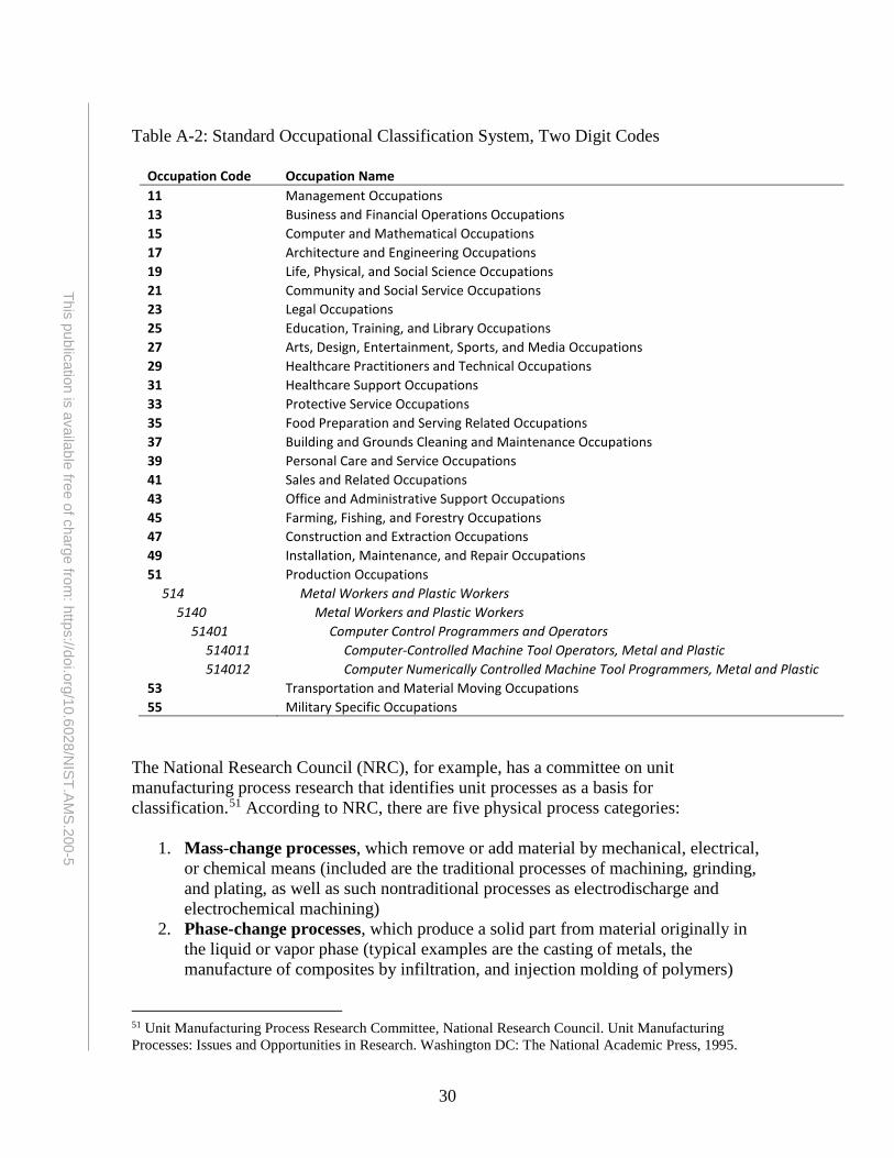
APPENDIX A A.1 Cost Categorization One challenge that is frequently faced in investment analyses is the standardization of data categories. A best practice is to use standardized costs. It aids in tracking costs throughout a firm. It is also applicable in situations where costs have to be estimated using industry-wide data. Industry and occupation classification systems can be useful as a basis for categorizing costs. Two major classification systems, the North American Industry Classification System (NAICS) and the Standard Occupational Classification system (SOC), are discussed below. These systems provide a standard for tracking costs across firms and supply chains. Additionally, using these systems makes it feasible to utilize industry level data when necessary, as it is often collected in these formats. Also discussed below is a categorization of processes, which does not have a format that is as widely recognized as the NAICS or SOC systems. A.2 Categorization of Services and Commodities Domestic data tends to be in the North American Industry Classification System (NAICS). It is the standard used by federal statistical agencies classifying business establishments in the United States. NAICS was jointly developed by the U.S. Economic Classification Policy Committee, Statistics Canada, and Mexico’s Instituto Nacional de Estadística y Geografía and was adopted in 1997.49 NAICS has several major categories each with subcategories. Historic data and some organizations continue to use the predecessor of NAICS, which is the Standard Industrial Classification system (SIC). NAICS codes are categorized at varying levels of detail. Table A-1 presents the lowest level of detail, which is the two digit NAICS. There are 20 categories. Additional detail is added by adding additional digits; thus, three digits provides more detail than the two digit and the four digit provides more detail than the three digit. The maximum is six digits, as illustrated for automobile manufacturing (NAICS 336111) and light truck and utility manufacturing (NAICS 336112). Sometimes a two, three, four, or five-digit code is followed by zeros, which do not represent categories. They are null or place holders. For example, the code 336000 represents NAICS 336. A.3 Labor Categorization Federal statistical agencies classify workers into occupational categories for collecting and distributing data on employees using the Standard Occupational Classification system (SOC). The 2010 version has 840 occupations. These are categorized into 23 major groups. Occupations with similar job duties, skills, categorized into 461 broad occupations, which are categorized into 97 minor groups, education, and/or training are grouped together. Similar to the NAICS codes, additional digits represent additional detail up to a maximum of six digits, as illustrated for SOC 514011 and SOC 514012 in Table A-2, which presents the 23 major groups. The SOC classifies all occupations in 49 US Census Bureau. North American Industry Classification System. <http://www.census.gov/eos/www/naics/>

29


IST.AM

S.200-5

which work is performed for pay or profit. It was first published in 1980, but was rarely utilized at that time. In 2000, it was revised and then again revised in 2010. The Bureau of Labor Statistics now publishes occupation data based on this system. Table A-1: North American Industry Classification System, Two Digit Codes

Sector Description 11 Agriculture, Forestry, Fishing and Hunting 21 Mining, Quarrying, and Oil and Gas Extraction 22 Utilities 23 Construction 31-33 Manufacturing

336 Transportation Equipment Manufacturing 3361 Motor Vehicle Manufacturing

33611 Automobile and Light Duty Motor Vehicle Manufacturing 336111 Automobile Manufacturing 336112 Light Truck and Utility Manufacturing

42 Wholesale Trade 44-45 Retail Trade 48-49 Transportation and Warehousing 51 Information 52 Finance and Insurance 53 Real Estate and Rental and Leasing 54 Professional, Scientific, and Technical Services 55 Management of Companies and Enterprises 56 Administrative and Support and Waste Management and Remediation Services 61 Educational Services 62 Health Care and Social Assistance 71 Arts, Entertainment, and Recreation 72 Accommodation and Food Services 81 Other Services (except Public Administration) 92 Public Administration

A.3 Process Categorization Thompson (2015) provides a convenient list of manufacturing processes (see Table A-3); however, the Thompson’s intention is not to provide a method of categorization.50 Manufacturing processes do not have a standard system of classification that is as widely known as NAICS or the SOC. There are, however, a number of classification schemes, as seen in Table A-4 which is taken from Mani et al. (2013). Each of the schemes shown have advantages and a different basis for classification. 50 Thompson, Rob. Manufacturing Processes for Design Professionals. New York, NY: Thames & Hudson, 2015.

30


IST.AM

S.200-5

Table A-2: Standard Occupational Classification System, Two Digit Codes

Occupation Code Occupation Name 11 Management Occupations 13 Business and Financial Operations Occupations 15 Computer and Mathematical Occupations 17 Architecture and Engineering Occupations 19 Life, Physical, and Social Science Occupations 21 Community and Social Service Occupations 23 Legal Occupations 25 Education, Training, and Library Occupations 27 Arts, Design, Entertainment, Sports, and Media Occupations 29 Healthcare Practitioners and Technical Occupations 31 Healthcare Support Occupations 33 Protective Service Occupations 35 Food Preparation and Serving Related Occupations 37 Building and Grounds Cleaning and Maintenance Occupations 39 Personal Care and Service Occupations 41 Sales and Related Occupations 43 Office and Administrative Support Occupations 45 Farming, Fishing, and Forestry Occupations 47 Construction and Extraction Occupations 49 Installation, Maintenance, and Repair Occupations 51 Production Occupations

514 Metal Workers and Plastic Workers 5140 Metal Workers and Plastic Workers

51401 Computer Control Programmers and Operators 514011 Computer-Controlled Machine Tool Operators, Metal and Plastic 514012 Computer Numerically Controlled Machine Tool Programmers, Metal and Plastic

53 Transportation and Material Moving Occupations 55 Military Specific Occupations

The National Research Council (NRC), for example, has a committee on unit manufacturing process research that identifies unit processes as a basis for classification.51 According to NRC, there are five physical process categories:

1. Mass-change processes, which remove or add material by mechanical, electrical, or chemical means (included are the traditional processes of machining, grinding, and plating, as well as such nontraditional processes as electrodischarge and electrochemical machining)

2. Phase-change processes, which produce a solid part from material originally in the liquid or vapor phase (typical examples are the casting of metals, the manufacture of composites by infiltration, and injection molding of polymers)

51 Unit Manufacturing Process Research Committee, National Research Council. Unit Manufacturing Processes: Issues and Opportunities in Research. Washington DC: The National Academic Press, 1995.

31


IST.AM

S.200-5

3. Structure-change processes, which alter the microstructure of a workpiece, either throughout its bulk or in a localized area such as its surface (heat treatment and surface hardening are typical processes within this family; the family also encompasses phase changes in the solid state, such as precipitation hardening)

4. Deformation processes, which alter the shape of a solid workpiece without changing its mass or composition (classical bulk-forming metalworking processes of rolling and forging are in this category, as are sheet-forming processes such as deep drawing and ironing)

5. Consolidation processes, which combine materials such as particles, filaments, or solid sections to form a solid part or component (powder metallurgy, ceramic molding, and polymer-matrix composite pressing are examples, as are joining processes, such as welding and brazing).

A more recognized taxonomy of processes is presented by Todd et al. (1994).52 Table A-5 presents a manufacturing process classification based on their taxonomy. For this report, a process code was developed similar to that of the NAICS and SOC and applied to their taxonomy. It is a six digit code where additional detail is added by adding additional digits; thus, three digits provides more detail than the two digit and the four digit provides more detail than the three digit. Unfortunately, the taxonomy presented by Todd et al is over 20 years old; therefore, there is, likely, a need to incorporate more recent developments for this taxonomy to be completely relevant. 52 Todd, Robert H., Dell K. Allen, and Leo Alting. Manufacturing Processes Reference Guide. New York, NY: Industrial Press, Inc, 1994. xiii-xxiv.

32


IST.AM

S.200-5

Table A-3: Manufacturing Process Categories

Category Process Category Process

Plas

tics a

nd R

ubbe

r

Blow molding

Laye

red

Additive manufacturing Thermoforming Rotation molding Vacuum casting Compression molding

Cutt

ing

Photochemical machining Injection molding Laser cutting Reaction injection molding Electrical discharge machining Dip molding Punching and blanking

Met

al

Panel beating Die cutting Metal spinning Water jet cutting Metal stamping Glass scoring Deep drawing

Join

ing

Arc welding Superforming Power beam welding Tube and section bending Friction welding swaging Vibration welding Roll forming Ultrasonic welding Forging Resistance welding Sand casting Soldering and brazing Die casting Staking Investment casting Hot plate welding Metal injection molding Joinery Electroforming Weaving Centrifugal casting Upholstery Press braking Timber frame structures

Glas

s and

Ce

ram

ics

Glassblowing

Fini

shin

g Te

chno

logy

Spray painting Lampworking Powder coating Clay throwing Anodizing Ceramic slip casting Electroplating Press molding ceramics Galvanizing

Woo

d

CNC machining (wood and other) Vacuum metalizing Wood laminating Grinding, sanding, and polishing Steam bending Electropolishing Paper pulp molding Abrasive blasting

Com

posit

es Composite laminating Photo etching

DMC and SMC molding CNC Engraving Filament winding Screen printing 3D Thermal laminating Pad printing

Hydro transfer printing Foil blocking and embossing

Source: Thompson, Rob. Manufacturing Processes for Design Professionals. New York, NY: Thames & Hudson, 2015.

33


IST.AM

S.200-5

Table A-4: Selection of Manufacturing Process Classifications

Source: Mani, Mahesh, Jatinder Madan, Jae Hyun Lee, Kevin W. Lyons, and Satyandra K. Gupta. 2013. Review on Sustainability Characterization for Manufacturing Processes. NISTIR 7913. http://nvlpubs.nist.gov/nistpubs/ir/2013/NIST.IR.7913.pdf

34


IST.AM

S.200-5

Table A-5: Manufacturing Process Classification (Based on Todd et al. 1994) Process Code Description Process Code Description 100000 Shaping 112330 Ion Beam Cutting 110000 Mass Reducing 113000 Chemical Reducing 111000 Mechanical Reducing 113100 Chemical Milling 111100 Reducing (chips) 113110 Immersion Chemical Milling 111110 Single-Point Cutting 113120 Spray Chemical Milling 111111 Turning/Facing 113200 Electrochemical Milling 111112 Boring 113210 Cavity-Type 111113 Shaping/Planing 113220 Grinder-Type 111114 Parting/Grooving 113300 Photochemical Milling 111115 Threading (SP) 113310 Photo Etching 111120 Multipoint Cutting 113320 Photo Milling 111121 Drilling 120000 Mass Conserving 111122 Reaming 121000 Consolidation 111123 Milling/Routing 121100 Casting - Nonreusable 111124 Broaching 121110 Ceramic Mold Casting 111125 Threading (MP) 121111 Investment Casting 111126 Filing 121112 Plaster Mold Casting 111127 Sawing 121120 Sand Mold Casting 111128 Gear Cutting 121121 Sand Casting 111130 Abrasive machining 121122 Shell Mold Casting 111131 Grinding 121123 No-Bake Mold Casting 111132 Honing 121124 Full-Mold Casting 111133 Lapping 121200 Casting - Reusable Mold 111134 Superfinishing 121210 Die Casting 111135 Ultrasonic Machining 121220 Permanent Mold Casting 111136 Jet Machining 121230 Flexible Mold Casting 111200 Seperating (shear) 121240 Continuous Casting 111210 Shearing 121300 Molding 111211 Squaring 121310 Ceramic Molding 111212 Slitting 121311 Wet Forming 111213 Rotary Shearing 121312 Dry Pressing 111214 Nibbling 121320 Polymer Molding 111220 Blanking 121321 Injection Molding 111221 Conventional Blanking 121322 Blow Molding 111222 Steel-Rule-Die Blanking 121323 Transfer Molding 111223 Fine Blanking 121324 Compression Molding 111224 Shaving/Trimming 121325 Extrusion Molding 111225 Dinking 121326 Thermoform Molding 111230 Piercing 121327 Rotational Molding 111231 Punching 121400 Compacting 111232 Perforating 121410 Continuous Compacting 111233 Lancing 121411 Powder Material Extrusion 111234 Notching 121412 Powder Material Rolling 112000 Thermal Reducing 121420 Noncontinuous Compacting 112100 Torch Cutting 121500 Deposition 112110 Air Arc Cutting 121510 Electroforming 112120 Gas Cutting 121600 Laminating 112130 Plasma Arc Cutting 121610 Filament Winding 112200 Electrical Discharge Machining (EDM) 121620 Sheet Laminating 112210 Cavity-Type 121630 Bulk Laminating 112220 Grinding 121631 Spray Lay-up 112230 Sawing 121632 Hand Lay-up 112300 High Energy Beam Machining 121640 Pultrusion 112310 Electron Beam Cutting 122000 Total Deformation 112320 Laser Beam Cutting 122100 Forging

35


IST.AM

S.200-5

Process Code Description Process Code Description 122110 Hot Forging 131200 Inertial Friction Welding 122111 Hammer Forging 131300 Ultrasonci Welding 122112 Drop Forging 131400 Explosive Welding 122113 Press Forging 132000 Thermal Joining 122114 Upset Forging 132100 Thermal Welding 122115 Roll Forging 132110 Electric Arc Welding 122120 Cold Forging 132111 Shielded Metal Arc Welding 122200 Extruding 132112 Gas Metal Arc (MIG) Welding 122210 Direct Extrusion 132113 Gas Tungsten Arc (TIG) Welding 122220 Indirect Extrusion 132114 Submerged Arc Welding 122230 Impact Extrusion 132115 Carbon Arc Welding 122300 Drawing 132116 Stud Welding 122310 Wire Drawing 132120 Electrical Resistance Welding 122320 Tube Drawing 132121 Spot Welding 122400 Rolling 132122 Seam Welding 122410 Sheet Rolling 132123 Projection Welding 122420 Foil Rolling 132124 Butt Welding 122430 Structural Rolling 132125 Percussion Welding 122440 Pierce Rolling 132126 Electroslag Welding 122500 Shear Spinning 132130 Gas/Chemical Welding 122600 Coining/Sizing/Hobbing 132131 Combustible Gas Welding 122700 Thread Forming 132132 Atomic Hydrogen Welding 122800 Knurling 132140 Braze Welding 123000 Local Deformation 132141 Gas Brazing 123100 Bending 132142 Carbon Arc Brazing 123110 Straight Angle Bending 132150 Diffusion Bonding 123120 Corrugation Bending 132160 High Energy Beam Welding 123130 Joggle Bending 132161 Electron Beam Welding 123140 Curling 132162 Laser Beam Welding 123150 Seaming 132163 Plasma Arc Welding 123160 Tube Bending 132200 Brazing 123170 Roll Forming 132210 Infrared Brazing 123200 Conventional Sheeting Forming 132220 Resistance Brazing 123210 Die Forming: Matched Die Drawing 132230 Torch Brazing 123211 Simple Rigid Die 132240 Dip Brazing 123212 Compound Die 132250 Furnace Brazing 123213 Progressive Die 132260 Induction Brazing 123220 Die Forming: Rubber Die Drawing 132300 Soldering 123221 Guerin Process 132310 Friction/Ultrasonic Soldering 123222 Martform Process 132320 Induction Soldering 123223 Hydroform Process 132330 Infrared Soldering 123230 Conventional Spinning 132340 Dip Soldering 123240 Stretch Forming 132350 Iron Soldering 123250 Embossing 132360 Resistance Soldering 123300 Conventional Tube Forming 132370 Torch Soldering 123310 Swaging 132380 Wave Soldering 123320 Flaring 133000 Chemical Joining: adhesive bonding 123330 Intraforming 200000 Nonshaping 123400 High Energy Rate Forming 210000 Heat Treatment 123410 Explosive Forming 212000 Annealing 123420 Electromagnetic Forming 212100 Recovery 123430 Electrohydraulic Forming 212110 Stress Relieving 130000 Joining 212120 Tempering 131000 Mechanical Joining 212200 Recrystallization 131100 Cold Pressure Welding 212210 Full Annealing

36


IST.AM

S.200-5

Process Code Description Process Code Description 212220 Process Annealing 222000 Surface Coating 212230 Short-Cycle Annealing 222100 Mechanical Coating 213000 Hardening 222110 Spray Coating: Pressure Transferred 213100 Surface Hardening 222111 Air Gun Spraying 213110 Carburizing 222112 High Pressure Airless Spray 213120 Chromizing 222120 Spray Coating: Charged Transferred 213130 Carbonitriding 222121 Electrostatic Coating 213140 Cyaniding 222122 Vacuum Coating 213150 Nitriding 222130 Dip/Flow Coating 213160 Diffusion Hardening 222131 Cold Dip Coating 213170 Flame Hardening 222132 Hot Dip Coating 213180 Induction Hardening 222133 Electrocoating 213200 Through Hardening 222134 Fluidized Bed Coating 213210 Water Quench Hardening 222135 Curtain Coating 213220 Oil Quench Hardening 222140 Dust Coating 213230 Air Quench Hardening 222150 Roll Coating 213240 Martempering 222151 Calendering 213250 Austempering 222152 Roller Coating 213260 Age Hardening 222200 Thermal Coating 214000 Other Heat Treatment 222210 Flame Spraying 214100 Sintering 222211 Combustion Flame Spraying 214110 Solid-Phase Sintering 222212 Plasma Arc Spraying 214120 Liquid-Phase Sintering 222213 Detonation Gun Spraying 214200 Subzero Cold Treatment 222220 Vaporized Metal Coating 214300 Firing/Glazing 222221 Vacuum Metallizing 214400 Curing/Bonding 222222 Sputtering 220000 Surface Finish 222223 Chemical Vapor-Phase Deposition 221000 Surface Preparation 222230 Heat Tinting 221100 Descaling 222300 Chemical Coating 221110 Mechanical Descaling 222310 Electroplating 221111 Abrasive Blasting 222320 Chemical Conversion 221112 Belt Sanding 222321 Anodize 221113 Shot Peening Preparation 222322 Alkaline Oxide 221114 Wire Brushing 222323 Fused Nitrate 221115 Grinding 222324 Proprietary Treatments 221120 Thermal Descaling 222325 Phosphate 221121 Flame Cleaning 222326 Chromate 221130 Chemical Descaling 223000 Surface Modification 221131 Chemical Pickling 223100 Burnishing 221200 Deburring 223200 Peening 221210 Mechanical Deburring 223210 Shot Peening 221211 Barrel Tumbling 223220 Hammer Peening 221212 Vibratory Finishing 223300 Texturing 221213 Knife Deburring 223310 Wire Brush Finishing 221220 Thermal Deburring 223320 Buffing/Polishing 221221 Thermochemical Deburring 221230 Chemical Deburring 221231 Electrochemical Deburring 221300 Degreasing 221310 Mechanical Degreasing 221311 Ultrasonic Degreasing 221320 Chemical Degreasing 221321 Vapor Degreasing 221322 Solvent Degreasing 221323 Alkali Degreasing

Source: Todd, Robert H., Dell K. Allen, and Leo Alting. Manufacturing Processes Reference Guide. New York, NY: Industrial Press, Inc, 1994. xiii-xxiv.

Investment Analysis Methods - nvlpubs.nist.gov · The scope of this guide is to provide assistance...

Documents

Transcript of Investment Analysis Methods - nvlpubs.nist.gov · The scope of this guide is to provide assistance...