INVESTIGATION ON CIRCUIT BREAKER INFLUENCE ON …szewczyk/pdf/papers/Conferences/M. Szewczyk et...
8
INVESTIGATION ON CIRCUIT BREAKER INFLUENCE ON TRANSIENT RECOVERY VOLTAGE Marcin Szewczyk, Stanislaw Kulas Warsaw University of Technology, Poland ABSTRACT As Hammarlund stated in [1], Transient Recovery Voltage (TRV) investigation can never be finished completely, as the progress of circuit breaker construction and network design goes on. The most common approach to TRV investigation is concerning the so called prospective TRV, in which an assumption of neglecting interaction between circuit breaker itself and the inherent system recovery voltage is being made. However, it still seems to be worthy to investigate how circuit breaker affects TRV. In presented paper such an influence is being investigated in some detail, with use of black- box Habedank circuit breaker model [2], in exemplary MV large industrial network [3]. The influence of reactance of inductive fault current limiter as well as distance to fault in short line fault condition on rate of rise of recovery voltage has been investigated. The investigation has been made by means of simulation performed using Matlab/Simulink programme. Keywords: transient recovery voltage, black-box circuit breaker modelling, short line fault, Matlab/Simulink. 1 MOTIVATION AND SCOPE OF THE PAPER In MV industrial networks power is being consume mostly by high voltage motors supplied by short cable lines, at attendance of fault current limiters (FCL) – with up to 80% share in exemplary networks investigated in [4, 5]. Short line faults (SLF) are characterized by much higher frequency range than terminal faults, reaches 100 kHz as reported in [6] and even higher as reported in [3]. Also, natural frequencies of FCL are much higher than those produced by system or transformer [6]. This frequency components are determining one of the most important factor of TRV severity, namely rate of rise of recovery voltage (RRRV), defined as u c /t 3 , where u c is peak value of TRV and t 3 is time parameter obtained from envelope of TRV as defined in [7] and depicted in Figure 1. This implies the importance of investigation on RRRV in SLF condition at attendance of FCL. Figure 1 Exemplary TRV shape with envelope. The scope of presented paper is to investigate how distance to fault in SLF condition and reactance of FCL influence RRRV, and how the model of circuit breaker that is used in simulation affects this influence. The simulation was performed with use of two models of circuit breaker: ideal and Habedank, as introduced in [2]. The second aim of presented paper is to extend the previous research group work, as the new research group has arisen in the field of TRV investigation in MV industrial networks at Warsaw University of Technology (WUT). For this reason, in section 2 the main papers of the previous group will be recall briefly on the background of TRV investigation methods. 2 TRV INVESTIGATION METHODS Transient recovery voltage has a great history of investigation, beginning in the early years of XX century. Presumably the first author [1] who gave a clear mathematical description of the phenomena was Slepian, in 1923 [8]. He found out that circuit breaker interrupting capacity is greatly affected by the system voltage natural oscillations, when current is interrupted after the instant of current zero. This TRV stresses the circuit-breaker gap when the gap conducts from the state of being good conductor to its normal condition of a good insulator. 2.1 Possible methods of investigation Since the Slepian work, plenty of methods have been developed to investigate TRV. In general, methods of investigations can be divided into two categories: measurement or calculation methods. The first ones are UPEC 2007 - 1036
Transcript of INVESTIGATION ON CIRCUIT BREAKER INFLUENCE ON …szewczyk/pdf/papers/Conferences/M. Szewczyk et...
INVESTIGATION ON CIRCUIT BREAKER INFLUENCE
ON TRANSIENT RECOVERY VOLTAGE
Marcin Szewczyk, Stanislaw Kulas
Warsaw University of Technology, Poland
ABSTRACT
As Hammarlund stated in [1], Transient Recovery Voltage (TRV) investigation can never be finished completely, as the
progress of circuit breaker construction and network design goes on. The most common approach to TRV investigation
is concerning the so called prospective TRV, in which an assumption of neglecting interaction between circuit breaker
itself and the inherent system recovery voltage is being made. However, it still seems to be worthy to investigate how
circuit breaker affects TRV. In presented paper such an influence is being investigated in some detail, with use of black-
box Habedank circuit breaker model [2], in exemplary MV large industrial network [3]. The influence of reactance of
inductive fault current limiter as well as distance to fault in short line fault condition on rate of rise of recovery voltage
has been investigated. The investigation has been made by means of simulation performed using Matlab/Simulink
programme.
Keywords: transient recovery voltage, black-box circuit breaker modelling, short line fault, Matlab/Simulink.
1 MOTIVATION AND SCOPE OF THE PAPER
In MV industrial networks power is being consume
mostly by high voltage motors supplied by short cable
lines, at attendance of fault current limiters (FCL) –
with up to 80% share in exemplary networks
investigated in [4, 5]. Short line faults (SLF) are
characterized by much higher frequency range than
terminal faults, reaches 100 kHz as reported in [6] and
even higher as reported in [3]. Also, natural frequencies
of FCL are much higher than those produced by system
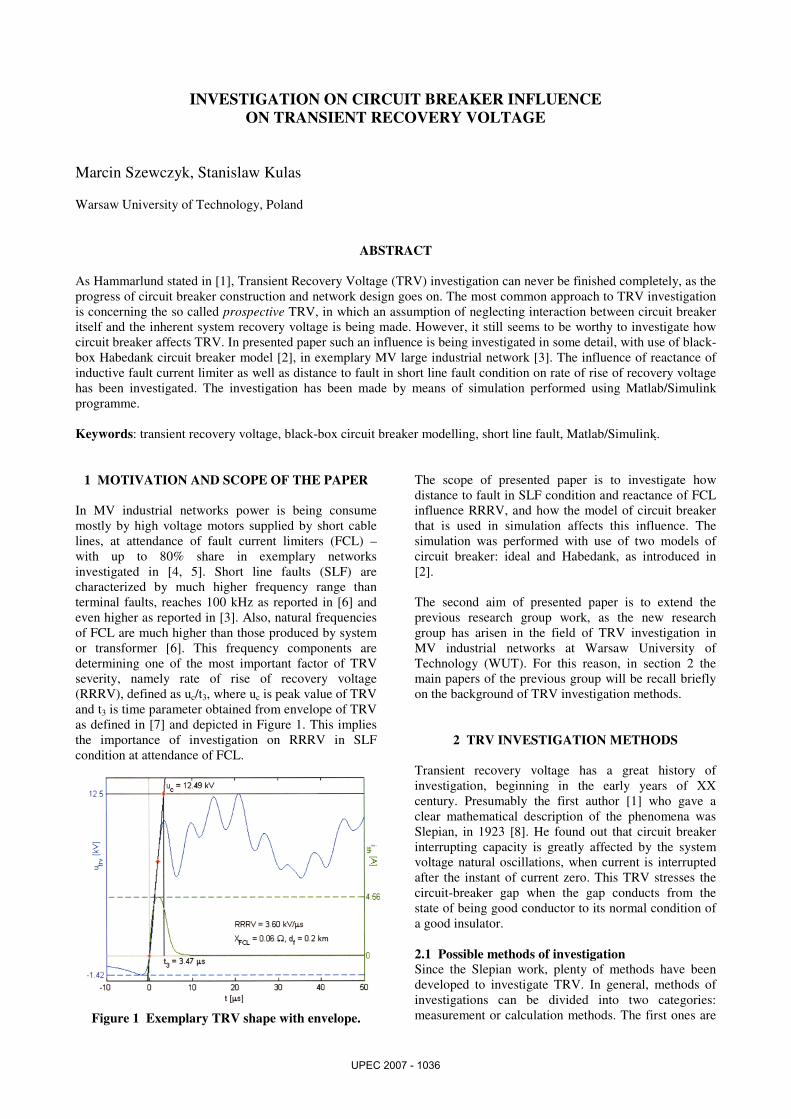
or transformer [6]. This frequency components are
determining one of the most important factor of TRV
severity, namely rate of rise of recovery voltage
(RRRV), defined as uc/t3, where uc is peak value of TRV
and t3 is time parameter obtained from envelope of TRV
as defined in [7] and depicted in Figure 1. This implies
the importance of investigation on RRRV in SLF
condition at attendance of FCL.
Figure 1 Exemplary TRV shape with envelope.
The scope of presented paper is to investigate how
distance to fault in SLF condition and reactance of FCL
influence RRRV, and how the model of circuit breaker
that is used in simulation affects this influence. The
simulation was performed with use of two models of
circuit breaker: ideal and Habedank, as introduced in
[2].
The second aim of presented paper is to extend the
previous research group work, as the new research
group has arisen in the field of TRV investigation in
MV industrial networks at Warsaw University of
Technology (WUT). For this reason, in section 2 the
main papers of the previous group will be recall briefly
on the background of TRV investigation methods.
2 TRV INVESTIGATION METHODS
Transient recovery voltage has a great history of
investigation, beginning in the early years of XX
century. Presumably the first author [1] who gave a
clear mathematical description of the phenomena was
Slepian, in 1923 [8]. He found out that circuit breaker
interrupting capacity is greatly affected by the system
voltage natural oscillations, when current is interrupted
after the instant of current zero. This TRV stresses the
circuit-breaker gap when the gap conducts from the
state of being good conductor to its normal condition of
a good insulator.
2.1 Possible methods of investigation
Since the Slepian work, plenty of methods have been
developed to investigate TRV. In general, methods of
investigations can be divided into two categories:
measurement or calculation methods. The first ones are
UPEC 2007 - 1036
appropriate only in those networks which already exist,
but they are the most accurate. This methods are
subdivided into two further categories: direct or indirect
methods, depending on how the measurements are being
taken: directly, by breaking short-circuit current, or
indirectly, by means of measuring some auxiliary
phenomena and hence conclude TRV in question. Some
of these methods require to operate on network whilst in
service, either fully or partially supplied, other methods
are intended to operate on dead network, either with or
without breaker action.
The second branch of the methods – calculation
methods – are more general than the measurement ones,
however they require a good knowledge of models of
network elements together with its parameters. In the
subject of modelling network elements, great effort has
already been done, hence there are plenty of known
models as well as modelling techniques for use in TRV
investigations. Some, but not obviously all of these
models have been successfully implemented in
commonly used numerical simulators, like ATP/EMTP
or Matlab/Simulink.
Obtaining network parameters is a great challenge of
calculation methods, and also – it brings the most share
to the methods accuracy. As it is often in case, the
knowledge of network parameters is greatly improved
when calculation methods are combined together with
measurement methods. In this category, an exemplary
method of [9] is worthy to be recalled. In this method,
network elements are being stimulated to their self
oscillations with their natural frequencies, caused by
application of the current-surge indicator. By
connecting additional capacitance or inductance on
terminals of the indicator during the measurements, the
changes of frequencies and amplitudes of oscillations
are to be observed, from which equivalent circuits
together with their parameters can be deduced.
2.2 TRV investigation in Polish MV
large industrial networks
Based on the later method mentioned above, the most
comprehensive investigation on TRV in Polish MV
large industrial networks has been made by Roguski in
1962 [10]. Further measurements performed by WUT
research group was published by Ciok in 1982 [4],
completed also by Ciok at al. in 1996 [3]. Since some
results from the latter papers have been used in
presented paper, it is worthy to mention that two of the
papers just recalled, namely [4, 10], had been used in
CIGRE report [11], concerning TRV in MV networks,
which is still in use nowadays [12] with reference to
TRV standardization. Presented paper extends the scope
of investigations reported in [3].
3 METHODOLOGY
The research reported in presented paper involves yet
another approach to TRV investigation, combining
measurement and calculation methods. In this approach,
not the TRV itself, but the influence of a certain
network element (i.e. cable, fault current limiter and
circuit breaker in that case) on a given prospective TRV
is being investigated.
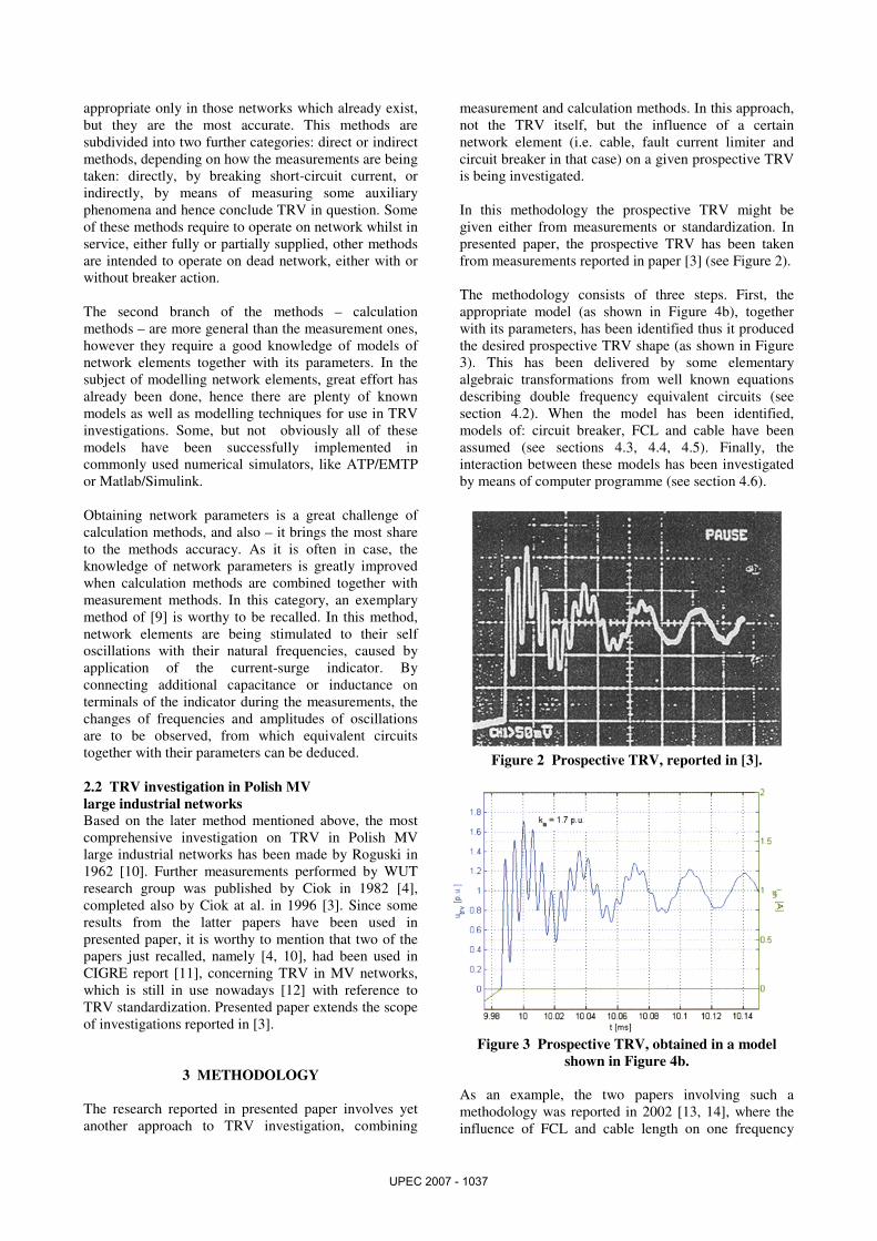
In this methodology the prospective TRV might be
given either from measurements or standardization. In
presented paper, the prospective TRV has been taken
from measurements reported in paper [3] (see Figure 2).
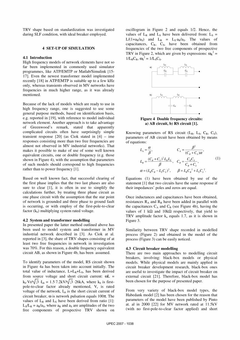
The methodology consists of three steps. First, the
appropriate model (as shown in Figure 4b), together
with its parameters, has been identified thus it produced
the desired prospective TRV shape (as shown in Figure
3). This has been delivered by some elementary
algebraic transformations from well known equations
describing double frequency equivalent circuits (see
section 4.2). When the model has been identified,
models of: circuit breaker, FCL and cable have been
assumed (see sections 4.3, 4.4, 4.5). Finally, the
interaction between these models has been investigated
by means of computer programme (see section 4.6).
Figure 2 Prospective TRV, reported in [3].
Figure 3 Prospective TRV, obtained in a model
shown in Figure 4b.
As an example, the two papers involving such a
methodology was reported in 2002 [13, 14], where the
influence of FCL and cable length on one frequency
UPEC 2007 - 1037
TRV shape based on standardization was investigated
during SLF condition, with ideal breaker employed.
4 SET-UP OF SIMULATION
4.1 Introduction
High frequency models of network elements have not so
far been implemented in commonly used simulator
programmes, like ATP/EMTP or Matlab/Simulink [15-
17]. Even the newest transformer model implemented
recently [18] in ATP/EMTP is suitable up to a few kHz
only, whereas transients observed in MV networks have
frequencies in much higher range, as it was already
mentioned.
Because of the lack of models which are ready to use in
high frequency range, one is suggested to use some
general purpose methods, based on identification basis,
e.g. reported in [19], with reference to model individual
network element. Another approach is to take advantage
of Greenwood’s remark, stated that apparently
complicated circuits often have surprisingly simple
transient response [20] (as Ciok stated in [4] – ime
responses consisting more than two free frequencies are
almost not observed in MV industrial networks). That
makes it possible to make of use of some well known
equivalent circuits, one or double frequency (e.g. those
shown in Figure 4), with the assumption that parameters
of such models should correspond to high frequencies
rather than to power frequency [1].
Based on well known fact, that successful clearing of
the first phase implies that the two last phases are also
sure to clear [1], it is often in use to simplify the
calculations further, by treating three phase circuit as
one phase circuit with the assumption that the star point
of network is grounded and three phase to ground fault
is occurring, or with employ of the first-pole-to-clear
factor (kb) multiplying system rated voltage.
4.2 System and transformer modelling
In presented paper the latter method outlined above has
been used to model system and transformer in MV
industrial network described in [3]. As Ciok at al.
reported in [3], the share of TRV shapes consisting of at
least two free frequencies in network in investigation
was 70%. For this reason, a double frequency equivalent
circuit AB, as shown in Figure 4b, has been assumed.
To identify parameters of the model, RS circuit shown
in Figure 4a has been taken into account initially. The
total value of inductance, L=LR+LS, has been derived
from source voltage and short circuit current: ωL =
kb⋅Vr/ ;3 ⋅Ish = 1.5⋅7.2kV/ ;3 ⋅26kA, where kb is first-
pole-to-clear factor already mentioned, Vr is rated
voltage of the network, Ish is the short circuit current of
circuit breaker, ω is network pulsation equals 100π. The
values of LR and LS have been derived from ratio [1]:
LS/LR = aR/aS, where aR and aS are amplitudes of the two
free components of prospective TRV shown on
oscillogram in Figure 2 and equals 1/2. Hence, the
values of LR and LS have been delivered from: LS =
L/(1+aR/aS) and LR = LS⋅aR/aS. The values of
capacitances, CR, CS, have been obtained from
frequencies of the two free components of prospective
TRV in Figure 2, which are given by expressions: ωR2 =
1/LRCR, ωS2 = 1/LSCS.
LR
CR
LS
CS
LA
CA
LB
CB
a)
b)
Figure 4 Double frequency circuits:
a) AB circuit, b) RS circuit [1].
Knowing parameters of RS circuit (LR, LS, CR, CS),
parameters of AB circuit have been obtained by means
of equations:
2
2
2 2 2
, ,( )
( ), ,
( ) , .
A A
R S
R S R S R SB B
R S
R R S S R R S S
L CC C
C C L L C CL C
C C
L C L C L C L C
α β
β α
β
α β
= =+
+= =
+
= − = +
(1)
Equations (1) have been obtained by use of the
statement [1] that two circuits have the same response if
their impedances’ poles and zeros are equal.
Once inductances and capacitances have been obtained,
resistances RA and RB have been added in parallel with
the capacitances CA and CB (see Figure 4b), having the
values of 1 kΩ and 10kΩ respectively, that yield to
TRV amplitude factor ka equals 1.7, as it is shown in
Figure 3.
Similarity between TRV shape recorded in modelled
process (Figure 2) and obtained in the model of the
process (Figure 3) can be easily noticed.
4.3 Circuit breaker modelling
There are two main approaches to modelling circuit
breakers, involving: black-box models or physical
models. While physical models are mainly applied in
circuit breaker development research, black-box ones
are useful to investigate the impact of circuit breaker on
external circuit [21]. Therefore, black-box model has
been chosen for the purpose of presented paper.
From very variety of black-box model types, the
Habedank model [2] has been chosen for the reason that
parameters of the model have been published by Pinto
at. al in 2000 [22] for MV network rated at 11.5kV
(with no first-pole-to-clear factor applied) and short
UPEC 2007 - 1038
circuit current equals 30 kA. Since values ;2/3 11.5kV
(in [22]) and 1.5⋅ ;2/3 7.2kV (in presented paper)
differs only in 6%, and short circuit currents differs in
15%, the values of arc parameters has been assumed to
be appropriate for the network in consideration.
Habedank model [2] of circuit breaker is constituted by
nonlinear, time varying conductance, described by
Cassie and Mayr equations:
2 2
2 2
2 2
1 11 ,
1 11 ,
1 1 1;
c
c c c c
m
m m o m
c m
dg u g
g dt U g
dg u g
g dt P g
g g g
τ
τ
= −
= −
= +
(2)
where: g – the total conductance of the arc, gc/gm – the
conductance of arc described by Cassie/Mayr equation,
τc/τm – the Cassie/Mayr time constant, Uc – the Cassie
constant arc voltage, P0 – the Mayr constant steady-state
power-loss of the arc.
The two serial conductances in the model plays
significant role in different phases of current
interrupting process. At high currents practically all the
voltage drop takes place in the Cassie portion of the
model [2]. In current zero crossing phase the voltage
drop on Mayr portion increases while the Cassie portion
goes to zero, which is consistent with Cassie and Mayr
models assumptions.
The values of model parameters are as follows [22]:
Uc = 200 V, Po = 70 kW, τc = 3 µs, τm = 1.1 µs.
For the purpose of model implementation, the approach
presented by Schavemaker at al. in 2002 [23] has been
applied (see section 4.6 and Figure 6).
For ideal circuit breaker model, a common ideal switch
implemented in Matlab/Simulink has been used. The
switch opens at first current-zero crossing after tripping
signal is given, conducing its resistance from value of
10 mΩ to 1 MΩ.
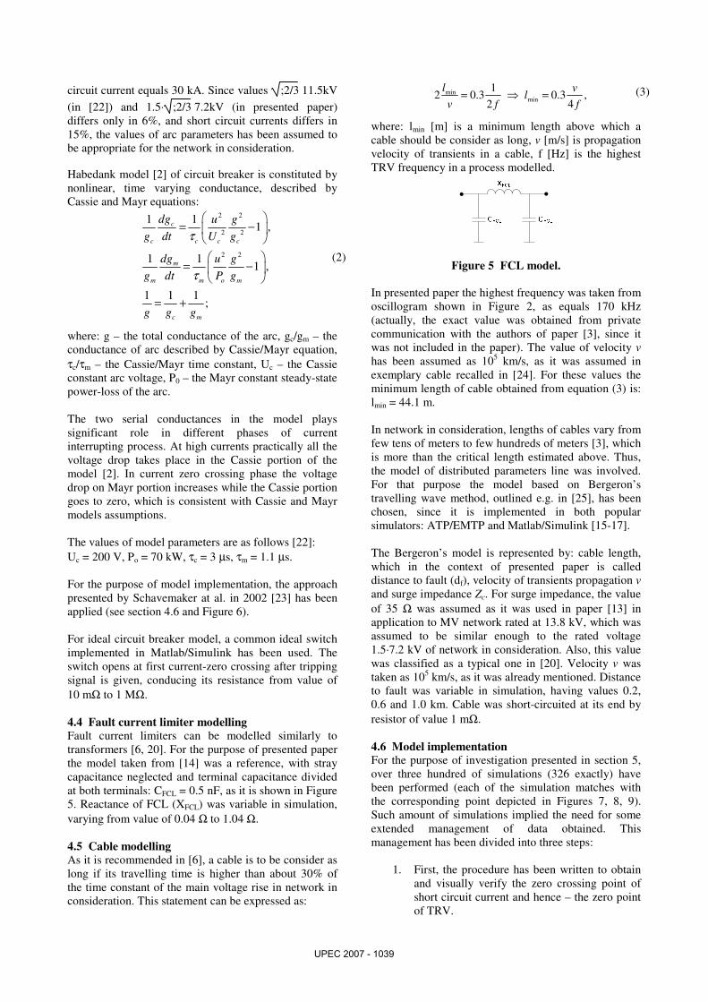
4.4 Fault current limiter modelling
Fault current limiters can be modelled similarly to
transformers [6, 20]. For the purpose of presented paper
the model taken from [14] was a reference, with stray
capacitance neglected and terminal capacitance divided
at both terminals: CFCL = 0.5 nF, as it is shown in Figure
5. Reactance of FCL (XFCL) was variable in simulation,
varying from value of 0.04 Ω to 1.04 Ω.
4.5 Cable modelling
As it is recommended in [6], a cable is to be consider as
long if its travelling time is higher than about 30% of
the time constant of the main voltage rise in network in
consideration. This statement can be expressed as:
minmin
12 0.3 0.3 ,
2 4
l vl
v f f= ⇒ = (3)
where: lmin [m] is a minimum length above which a
cable should be consider as long, v [m/s] is propagation
velocity of transients in a cable, f [Hz] is the highest
TRV frequency in a process modelled.
Figure 5 FCL model.
In presented paper the highest frequency was taken from
oscillogram shown in Figure 2, as equals 170 kHz
(actually, the exact value was obtained from private
communication with the authors of paper [3], since it
was not included in the paper). The value of velocity v
has been assumed as 105 km/s, as it was assumed in
exemplary cable recalled in [24]. For these values the
minimum length of cable obtained from equation (3) is:
lmin = 44.1 m.
In network in consideration, lengths of cables vary from
few tens of meters to few hundreds of meters [3], which
is more than the critical length estimated above. Thus,
the model of distributed parameters line was involved.
For that purpose the model based on Bergeron’s
travelling wave method, outlined e.g. in [25], has been
chosen, since it is implemented in both popular
simulators: ATP/EMTP and Matlab/Simulink [15-17].
The Bergeron’s model is represented by: cable length,
which in the context of presented paper is called
distance to fault (df), velocity of transients propagation v
and surge impedance Zc. For surge impedance, the value
of 35 Ω was assumed as it was used in paper [13] in
application to MV network rated at 13.8 kV, which was
assumed to be similar enough to the rated voltage
1.5·7.2 kV of network in consideration. Also, this value
was classified as a typical one in [20]. Velocity v was
taken as 105 km/s, as it was already mentioned. Distance
to fault was variable in simulation, having values 0.2,
0.6 and 1.0 km. Cable was short-circuited at its end by
resistor of value 1 mΩ.
4.6 Model implementation
For the purpose of investigation presented in section 5,
over three hundred of simulations (326 exactly) have
been performed (each of the simulation matches with
the corresponding point depicted in Figures 7, 8, 9).
Such amount of simulations implied the need for some
extended management of data obtained. This
management has been divided into three steps:
1. First, the procedure has been written to obtain
and visually verify the zero crossing point of
short circuit current and hence – the zero point
of TRV.
UPEC 2007 - 1039
2. Then the procedure has been written to obtain
and visually verify TRV envelope, and its
parameters such as RRRV, as it is shown in
Figure 1.
3. Finally, all the data was stored in data base for
the purpose of plotting selected results later on.
As Greenwood stated in [20], EMTP had become a kind
of cult in the electric power industry. This situation
seems to last nowadays, hence ATP/EMTP was chosen
as a reference to justify the choice of Matlab/Simulink
in presented paper.
In paper [26] same advantages and disadvantages of
Matlab/Simulink versus ATP/EMTP has been
discussed, from which two are worth to mention in the
context of procedures listed above. The main advantage
of Matlab/Simulink from this point of view is its open
code structure – user is able to write almost any
mathematical and logical procedure, even based on
modern object oriented basis. This implies
Matlab/Simulink is much more flexible in use than
ATP/EMTP. The main advantage of ATP/EMTP in turn
might be its nodal approach to network analysis
contrary to the state-space approach involved in
Matlab/Simulink. This implies ATP/EMTP is faster for
large scale systems (see discussion in [26]).
Since model involved in presented paper has only up to
ten state variables, whereas extended data management
was needed as it was mentioned, Matlab/Simulink has
been chosen as more suitable for the model
implementation.
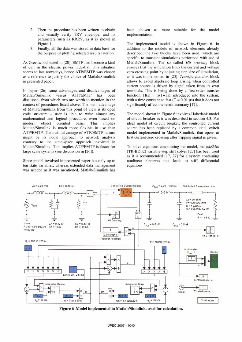
The implemented model is shown in Figure 6. In
addition to the models of network elements already
described, the two blocks have been used, which are
specific to transient simulations performed with use of
Matlab/Simulink. The so called Hit crossing block
ensures that the simulation finds the current and voltage
zero crossing point by adjusting step size of simulation,
as it was implemented in [23]. Transfer function block
allows to avoid algebraic loop arising when controlled
current source is driven by signal taken from its own
terminals. This is being done by a first-order transfer
function, H(s) = 1/(1+Ts), introduced into the system,
with a time constant so fast (T = 0.01 µs) that it does not
significantly affect the result accuracy [17].
The model shown in Figure 6 involves Habedank model
of circuit breaker as it was described in section 4.3. For
ideal model of circuit breaker, the controlled current
source has been replaced by a common ideal switch
model implemented in Matlab/Simulink, that opens at
first current-zero crossing after tripping signal is given.
To solve equations constituting the model, the ode23tb
(TR-BDF2) variable-step stiff solver [27] has been used
as it is recommended [17, 27] for a system containing
nonlinear elements that leads to stiff differential
equations.
Figure 6 Model implemented in Matlab/Simulink, used for calculation.
UPEC 2007 - 1040

5 RESULTS OF INVESTIGATION
Results of investigation are presented in Figures 7, 8, 9.
Figure 7 shows how RRRV depends on reactance of
FCL (XFCL) and distance to fault (df). Simulations were
performed with use of both circuit breaker models: ideal
(marked as Alpha) and Habedank, for three distances to
fault. As it is shown in Figure 7, for ideal model RRRV
initially increases and then decreases, while for
Habedank model RRRV increases in whole range of
XFCL, reaches a plateau finally. For both models, the
shorter distance to fault implies the higher RRRV.
Figure 7 RRRV versus XFCL
for different distances to fault df and both: ideal
(Alpha) and Habedank circuit breaker model.
The variation of RRRV with distance to fault can be
explained by the saw tooth component of TRV related
with cable [20]. Since its base frequency is given by
expression: f = v/4/df, the shorter distance to fault is, the
higher frequency is, hence the higher RRRV emerges.
The variation of RRRV with reactance of FCL (XFCL)
for ideal circuit breaker can be explained as follows. For
small values of XFCL, the frequency of FCL component
of TRV, given by expression f = 1/2/π/ ;XFCLCFCL/ω ,
is much higher than those of AB circuit and cable
components. At that time, the amplitude of the FCL
component is neglected in comparison with AB and
cable components, because of the small value of XFCL.
Hence RRRV results from AB and cable components
only. When the value of XFCL increases, frequency of
related component decreases, but it is still much higher
than those of the remaining components. As the
amplitude of FCL component increases with XFCL
growth, it brings more and more share in resultant TRV,
and hence RRRV increases, reaches its maximum value
for a certain value of XFCL (approximately 0.2 Ω in that
case). For this value, the FCL component of TRV
become such a dominant in comparison with remaining
components, that it entirely determines the character of
TRV. Now the rule of decreasing RRRV with
decreasing frequency of FCL component is working,
since practically only this component remains. In
consequence, RRRV decreases with XFCL growth.
Figure 8 shows how RRRV depends on individual
parameters of Habedank circuit breaker model, for
distance to fault (df) equals 0.2 km and reactance of
FCL (XFCL) equals 0.32 Ω. The values of parameters
were deviated in the range of 20%. Because of great
difference in significance between individual
parameters, the values were plotted in two subplots.
Figure 8 Contribution to influence of individual
parameters of Habedank model on RRRV;
P0 = 70 kW, ττττm0 = 1.1 µµµµs, Uc0 = 200 V, ττττc0 = 3 µµµµs,
XFCL = 0.32 ΩΩΩΩ, df = 0.2 km, RRRV0 = 5. 39 kV/µµµµs.
Figure 9 shows how RRRV depends on reactance of
FCL (XFCL) when Habedank circuit breaker model was
employed for different values of Mayr-part parameters
of the model.
Figure 9 RRRV versus XFCL for Mayr-part model
parameters; df = 0.2 km, P0 = 70 kW, tm0 = 1.1 µµµµs.
UPEC 2007 - 1041

6 CONCLUSIONS
The objective of presented paper was to investigate how
circuit breaker model affects transient recovery voltage
(TRV). As a parameter characterizing severity of TRV,
rate of rise of recovery voltage (RRRV) has been
chosen.
Secondary aim of the paper was to contribute
continuation of research in Polish MV large industrial
networks began by Roguski and Ciok at Warsaw
University of Technology. For that purpose, the case of
MV network described in [3] has been chosen to
perform identification of parameters of network model.
While MV large industrial network has been taken
under consideration, the problem of breaking short
circuit current in short line fault (SLF) condition at
presence of inductive fault current limiter (FCL) has
been chosen to investigate.
Attention was pointed at the influence of distance to
fault (df) and reactance of fault current limiter (XFCL) on
RRRV. The simulation was carried with use of two
different circuit breaker models: ideal (marked as
Alpha) and Habedank, implemented in Matlab/Simulink
programme.
Results of simulations are shown in Figures 7, 8, 9. The
following conclusions can be stated:
1. The shorter distance to fault is, the higher
value of RRRV is, regardless of what circuit
breaker model has been involved (Figure 7).
2. RRRV versus reactance of FCL increases and
then decreases for ideal circuit breaker, while
increases and then reaches a plateau for
Habedank circuit breaker model (Figure 7).
Thus it has been shown that application of
circuit breaker model might significantly
change character of correlation between RRRV
and XFCL when simulated by means of
commonly used modelling techniques.
3. In Habedank model of circuit breaker four
parameters exist, from which only those related
with Mayr-part of the model have significant
influence on RRRV, whereas those related
with Cassie-part have negligible influence on
RRRV in the case of interest (Figure 8). The
current zero crossing phase is crucial in
Habedank model in that case.
4. The most significant contribution to RRRV in
Habedank circuit breaker model is brought by
Mayr time constant τm (Figures 8, 9).
7 ACKNOWLEDGMENT
The authors acknowledge to Polish State Committee for
Scientific Research the contribution of this work
financed as granted research project No. N510 004
32/0358.
8 REFERENCES
1. Hammarlund, P., Transient recovery voltage
subsequent to short circuit interruption with special
reference to Swedish power systems. 1946,
Stockholm: Ingeniörsvetenskapsakademiens
Handlingar Nr. 189.
2. Habedank, U., Application of a New Arc Model for
the Evaluation of Short-circuit Breaking Tests. IEEE
Transactions on Power Delivery, 1993. 8(4): p.
1921-1925.
3. Ciok, Z., et al. Transient Recovery Voltages in
Selected Medium Voltage Networks. in CIGRE.
1996.
4. Ciok, Z., Transient Recovery Voltages in Large
Industrial Networks. Acta Polytechnica (CVUT -
Technical University of Prague) (in English), 1982.
20: p. 75-82.
5. Ciok, Z. Overvoltages in industrial networks. in
Athens Power Tech Conference "Planning Operation
and Control of Today's Electric Power Systems",
vol. 2, pp. 946-949. September 5-8, 1993.
6. CIGRE-WG33.02, Guidelines for representation of
network elements when calculating transients.
CIGRE Brochure 39, 1990.
7. Standard, IEC 62271-100. High-voltage switchgear
and controlgear – Part 100: Highvoltage
alternating-current circuit breakers. 2001, IEC. p.
340.
8. Slepian, J., Extinction of an A-C Arc. Transactions
AIEE, 1928. 47(4): p. 1398-1407.
9. Roguski, A., Method of Determination of Restriking
Voltages by Measuring the Local Restriking
Voltages (in Polish). Archiwum Elektrotechniki,
1960. 9(1): p. 157-202.
10. Roguski, A., Investigations of Restriking Voltages in
Polish Networks (in Polish). Prace Instytutu
Elektrotechniki. Transactions of the Electrotechnical
Institute., 1962. 30: p. 1-46.
11. CIGRE-WG13.01, Transient recovery voltage in
medium voltage networks. CIGRE Working Group
13-01 Technical Brochure 134, December 1989. 88:
p. 49-88.
12. CIGRE-A3.11, Guide for Application of IEC 62271-
100 and IEC 62271-1 304. Part 1 - General
Subjects. 2006. p. 107.
13. Dufournet, D. and G.F. Montillet, Transient
Recovery Voltages Requirements for System Source
Fault Interrupting by Small Generator Circuit
Breakers. IEEE Transactions on Power Delivery,
2002. 17(2): p. 474-478.
14. Calixte, E., et al., Interrupting Condition Imposed on
a Circuit Breaker Connected with Fault Limiter.
International Journal of Power & Energy Systems,
2002. 25(2): p. 75-81.
15. Prikler, L. and H.K. Hoidalen, ATPDraw User's
Manual. 2002: SINTEF Report, No. F5680.
UPEC 2007 - 1042

16. Dommel, H.W., Electromagnetic Transients
Program (EMTP) Theory Book. 1987, Portland,
Oregon: Boneville Power Administration.
17. Mathworks, SimPowerSystems for use with
SIMULINK, Modeling, Simulation, Implementation -
User's Guide, Version 4. 2006: The Mathworks Inc.,
24 Prime Park Way, Natick. MA 01760-1500. 1154.
18. Mork, B.A., et al., Hybrid Transformer Model for
Transient Simulation - Part I: Development and
Parameters. IEEE Transactions on Power Delivery,
2007. 22(1): p. 248-255.
19. Morched, A., L. Marti, and J. Ottevangers, A High
Frequency Model Transformer for the EMTP. IEEE
Transactions on Power Delivery, 1993. 8(3): p.
1615-1626.
20. Greenwood, A., Electrical Transients in Power
Systems. 1991: John Wiley & Sons, Inc.
21. CIGRE-WG13.01, Practical Application of Arc
Physics in Circuit Breakers. Survey of Calculation
Methods and Application Guide. Electra, 1988. 118:
p. 66-79.
22. Pinto, L.C. and L.C.J. Zanetta, Medium voltage SF6
circuit-breaker arc model application. Electric
Power Systems Research, 2000. 53: p. 67-71.
23. Schavemaker, P.H. and L. Sluis. The Arc Model
Blockset. in The Second IASTED International
Conference: Power and Energy Systems (EuroPES).
2002. Crete, Greece.
24. Sluis, L., Transients in Power Systems. 2001: John
Wiley & Sons, Inc.
25. Henschel, S., A.I. Ibrahim, and H.W. Dommel,
Transmission Line Model for Variable Step Size
Simulation Algorithms. Electrical Power and Energy
Systems, 1999. 21: p. 191-198.
26. Mahseredjian, J. and F. Alvarado, Creating an
Electromagnetic Transients Program in MATLAB:
MatEMTP. IEEE Transactions on Power Delivery,
1997. 12(1): p. 380-388.
27. Hosea, M.E. and L.F. Shampine, Analysis and
implementation of TR-BDF2. Applied Numerical
Mathematics, 1996. 20(1): p. 21-37.
AUTHORS ADDRESS
The first author can be contacted at
Warsaw University of Technology
Department of High Voltage Engineering
and Electrical Apparatus
00-662 Warsaw, Koszykowa 75, Poland
e-mail: [email protected]
UPEC 2007 - 1043