Investigation of the Implementation of Ramp Reversal at A ...

INVESTIGATION OF THE IMPLEMENTATION OF RAMP REVERSAL AT A

DIAMOND INTERCHANGE

A Thesis

by

BO WANG

Submitted to the Office of Graduate Studies of Texas A&M University

in partial fulfillment of the requirements for the degree of

MASTER OF SCIENCE

Chair of Committee, Yunlong Zhang

Committee Members, Bruce Wang Clifford Spiegelman Head of Department, John Niedzwecki

August 2013

Major Subject: Civil Engineering

Copyright 2013 Bo Wang

ii

ABSTRACT

Diamond interchange design has been commonly utilized in United States to

facilitate traffic exchange between freeway and frontage roads. Another less common

interchange design is X-ramp interchange, which is the reversed version of diamond.

The major benefit of X-ramp interchange is that it can keep travelers on the freeway

until the downstream exit ramp to avoid going through the intersection. It also has

drawbacks such as travelers with cross street destinations will experience more delay.

This study focuses on when the ramp reversal is desirable. To compare the diamond and

X-ramp design, an experimental design is conducted using Latin Hypercube Design

method. Four varying factors include interchange design type, traffic volume on the

frontage road, through movement percentage and saturation rate of the intersection. 40

scenarios are generated for simulation study using Synchro and VISSIM.

Based on the simulation study, optimal signal timing strategies are recommended

for each type of interchange design under various traffic conditions. Also, ramp reversal

is found closely related to the following factors such as interchange frequency, upstream

interchange design, traffic volume on frontage road, through movement percentage and

intersection saturation rate. Conclusions are made on when X-ramp is better than

diamond interchange design. At last, future research directions are recommended.

iii

ACKNOWLEDGEMENTS

I would like to thank my committee chair, Dr. Zhang, and my committee

members, Dr. Spiegelman and Dr. Wang for their guidance and support throughout the

course of this research.

Thanks also go to my friends and colleagues and the department faculty and staff

for making my time at Texas A&M University a great experience. I also want to extend

my gratitude to the Texas Transportation Institute, which provided the survey data of SH

6 @ Harvey Rd interchange for simulation model development in this study.

Finally, thanks to my mother and father for their encouragement, patience and

love.

iv

TABLE OF CONTENTS

Page

ABSTRACT .............................................................................................................. ii

ACKNOWLEDGEMENTS ...................................................................................... iii

TABLE OF CONTENTS .......................................................................................... iv

LIST OF FIGURES ................................................................................................... vi

LIST OF TABLES .................................................................................................... vii

CHAPTER I INTRODUCTION ............................................................................ 1

1.1 Diamond Interchange and X-ramp Interchange ............................................ 1 1.2 Research Motivations .................................................................................... 2 1.3 Problem Statement ........................................................................................ 4 1.4 Research Objectives ...................................................................................... 5 1.5 Thesis Organization ....................................................................................... 6

CHAPTER II LITERATURE REVIEW ................................................................ 8

2.1 Signal Timing Strategies for Diamond Interchange ...................................... 8 2.2 Diamond Interchange Operation ................................................................... 9 2.3 Microscopic Simulation ................................................................................ 10 2.4 Ramp Reversal .............................................................................................. 12

CHAPTER III MICROSCOPIC SIMULATION ............................................... 15

3.1 Microscopic Traffic Simulation Software - VISSIM .................................... 15 3.2 Simulation Data ............................................................................................. 16 3.3 Simulation Model Development ................................................................... 18 3.4 Simulation Model Calibration ....................................................................... 27

CHAPTER VI SIGNAL TIMING OPTIMIZATION ........................................ 38

4.1 Optimization Tool -- Synchro ....................................................................... 39 4.2 Signal Timing Strategies ............................................................................... 39

4.3 Cycle Length Optimization ........................................................................... 41 4.4 Phase Split Optimization ............................................................................... 42

v

Page

4.5 Left Turn Treatment ...................................................................................... 42 4.6 Case Study Example ...................................................................................... 43

CHAPTER V MODEL ANALYSIS ..................................................................... 45

5.1 Experimental Design ..................................................................................... 45 5.2 Simulation Runs for Each Scenario .............................................................. 52 5.3 Additional Factors ......................................................................................... 53 5.4 Simulation Results ......................................................................................... 54

CHAPTER VI CONCLUSION AND RECOMMENDATIONS ........................... 68

6.1 Signal Timing Strategy Conclusions ............................................................. 68 6.2 Ramp Reversal Conclusions .......................................................................... 69 6.3 Future Research Recommendations .............................................................. 70

REFERENCES .......................................................................................................... 71

vi

LIST OF FIGURES

FIGURE Page

1 Conventional Diamond Interchange Layout .............................................. 1 2 X-Ramp Interchange Layout ...................................................................... 2 3 SH6 @ Harvey Road Interchange ............................................................. 17 4 Background Settings in VISSIM ................................................................ 19 5 Links in VISSIM ........................................................................................ 20 6 Connectors in VISSIM ............................................................................... 21 7 Vehicle Inputs in VISSIM .......................................................................... 22 8 Vehicle Types in VISSIM .......................................................................... 23 9 Routes in VISSIM ...................................................................................... 24 10 Signal Controllers in VISSIM .................................................................... 25 11 Priority Rule in VISSIM ............................................................................ 26 12 Driving Behavior Parameters in VISSIM .................................................. 27 13 Initial Evaluation Using Default Parameters .............................................. 34 14 Three-Phase Operations ............................................................................. 40 15 Four-Phase Operations ............................................................................... 41 16 Network Information in Synchro ............................................................... 43 17 Signal Timing Plan for the SH6 @ Harvey Rd Interchange ...................... 44 18 Diamond Interchange Movement/Phase .................................................... 46

vii

LIST OF TABLES

TABLE Page 1 Adjustable Parameters in VISSIM ............................................................. 28 2 Paired t-test Results for Analysis of Sensitivity ......................................... 31 3 Sensitive Parameters and Acceptable Range.............................................. 35 4 Parameter Sets Generate by LHS Method .................................................. 36 5 Calibrated Parameters Using GA ............................................................... 37 6 Summary of the Optimization Procedure ................................................... 44 7 Factors in Experimental Design ................................................................. 47 8 Latin Hypercube Design ............................................................................. 48 9 Simulation Scenarios Summary ................................................................. 49 10 Summary of Initial Runs ............................................................................ 53 11 Summary of Signal Timing Strategies ....................................................... 55 12 Summary of VISSIM Results ..................................................................... 57 13 Revised Results for X-ramp Interchange .................................................. 61 14 Comparison Results 1 ................................................................................. 65 15 Comparison Results 2 ................................................................................. 66 16 Comparison Results 3 ................................................................................. 67

1

CHAPTER I

INTRODUCTION

1.1 Diamond Interchange and X-ramp Interchange

An interchange is a road junction that typically uses grade separation, and one or more

ramps, to permit traffic on at least one highway to pass through the junction without

directly crossing any other traffic stream (Chlewicki, 2003). Diamond interchange design

is often utilized in Texas to facilitate traffic exchange between freeway and frontage

road. In a conventional diamond interchange design, or Y-ramp interchange, exit ramp is

located upstream of an entrance ramp. Figure 1 shows the shape of two diamond

interchange, from which we can find that this type of interchange design get its name

because it shapes like a diamond.

Figure 1 Conventional Diamond Interchange Layout (Not to Scale).

2

Eventually, researchers realized that in some scenarios, it would be beneficial to reverse

the exit ramp or the entrance ramp. Ramp reversal is defined as to replace an exit ramp

with an entrance ramp or vice versa. If all four ramps in a typical diamond interchange

are reversed, then it becomes an X-ramp interchange. Figure 2 shows the shape of X-

ramp interchanges. In an X-ramp interchange, the exiting ramp locates at the

downstream of the entrance ramp, which is just the opposite of a diamond interchange.

And this is the main difference between those two interchange design types in terms of

geometry.

Figure 2 X-Ramp Interchange Layout (Not to Scale)

1.2 Research Motivations

Population growth and vehicle ownership increase has placed tremendous burden on

freeway systems, especially in urban areas. The cost of constructing new facilities or

expanding existing ones has become too expensive to afford. When road expansion

3

becomes less possible, many states’ Department of Transportation (DOT) tries to seek

for new approach to maximize freeway capacity and efficiency. Modification of current

freeway elements is one way of avoiding high construction cost while resolving traffic

congestion. One important and effective approach is to modify ramp configurations via

ramp relocations and ramp reversal. It often can help reduce vehicle queues at critical

locations, redirect traffic to avoid signals, and thus mitigate roadway congestions. One

common way of ramp modification is ramp reversal at diamond interchanges.

Diamond interchange design is widely used throughout United States to facilitate vehicle

exchanges between freeway and frontage road. However, diamond interchange design

has its drawbacks such as heavy demand on frontage road, queue storage issue between

exit ramp and signalized intersection, etc. Some researchers believed that through ramp

reversal or ramp relocation, such problems could be resolved. To better investigate the

benefit of ramp reversal, theoretical and practical studies had been conducted by

researchers at Texas Transportation Institute (Cooner, 2007). Nevertheless, the problem

of when and where to use an X-ramp design as opposed to the more conventional

diamond ramp design for freeway interchange has not been resolved adequately.

No existing research has been found engaging on the investigation of traffic demand and

pattern’s impact on interchange design type selection. However, the major difference

between diamond interchange and x-ramp interchange is reflected on accessing the

nearby facilities. The most beneficial part of X-ramp design comparing to diamond is its

4

capability of removing the traffic load at several upstream locations without requiring

motorists to pass through a series of signalized intersections. Thus, to determine which

design to use, the major issue is to investigate the demand conditions around the

interchange.

1.3 Problem Statement

One of the major benefits of X-ramp interchange is to allow vehicles to avoid the

signalized intersection on frontage road, and thus dramatically decrease control delay.

However, to ensure this benefit, the destination of the vehicle has to be located

downstream of the signalized intersection. If its destination is located upstream, then

such maneuver is undesirable. Therefore, the major factors that determine which type of

interchange is beneficial are traffic demand pattern and demand level. While the

previous studies by TTI researchers tried to develop guidelines for ramp reversal

projects, little effort has been carried out to find the traffic demand’s influence on

interchange design. Also, no signal timing strategies were recommended for the reversed

diamond interchange design.

A microscopic simulation analysis should be conducted to compare both interchange

designs under different traffic demand scenarios. This simulation technique mimics the

real world situation on a computer, gives the flexibility of different scenario designs, and

offers the opportunity of projecting the consequence of the alternatives even before

actual implementation. In addition, it is time and cost efficient, and risk-free. Thus, this

5

research is designated to determine the benefits of ramp reversal under different

scenarios with the help of simulation, and in what kind of demand conditions, ramp

reversal is desirable. Plus, the researcher will investigate different interchange signal

timing strategies to find out the one that suits X-ramp design the best.

1.4 Research Objectives

The main goal of this study is to determine when and where an X-ramp interchange

design is more desirable than the conventional diamond interchange design by analyzing

the influence of traffic demand pattern on interchange operations using microscopic

simulation technique. The research objectives are:

To model the existing diamond interchange using microscopic simulation software

and to calibrate the model using field data,

To use the model to simulate traffic operation conditions of an X-ramp interchange

by reversing ramps,

To vary the traffic demand pattern and demand level in the model and analyze the

effect of different flow ratios on interchange operations, and

To recommend the optimal signal timing strategies for X-ramp interchange design

under various scenarios, and

To identify the cost and benefit of ramp reversal under various conditions in

financial units, and

To make a recommendation on when a ramp reversal is desirable under different

flow patterns and flow levels.

6

1.5 Thesis Organization

Chapter 1 introduces some basic concepts that will be discussed in this research such as

diamond interchange, X-ramp interchange and ramp reversal. This chapter also states the

research motivation and the problem that has been studied, and the objectives of this

research.

Chapter 2 will summarize background information and previous researches about signal

timing strategies for diamond interchange, diamond interchange operations, and ramp

reversal.

Chapter 3 will introduce the microscopic traffic simulation software – VISSIM.

Procedures and data used to develop the simulation model in VISSIM will be

demonstrated. Calibration process of the model will be shown.

Chapter 4 will introduce the signal timing optimization software – Synchro, and the

procedures to optimize signal timing plan.

Chapter 5 will introduce the Latin Hypercube Design method used to conduct

experimental design. It also will show how the number of simulation runs for each

scenario is determined. Plus, the simulation results from Synchro and VISSIM will be

shown and discussed.

7

Chapter 6 will conclude what has been done and recommend the optimal signal timing

strategy for each scenario. Essential factors that will influence the selection of a diamond

design or an X-ramp design will be explained. Future research recommendations also

will be made.

8

CHAPTER II

LITERATURE REVIEW

2.1 Signal Timing Strategies for Diamond Interchange

Being the most popular interchange design in U.S., diamond interchange operation has

been extensively studied by numerous researchers. Messer and Berry (1975) examined

the effects of minimum phase length and variations in spatial arrangement of ramp

intersections on the capacity of diamond interchanges operated with 4-phase-overlap

signalization. The FORTRAN IV was developed for their analysis, and they found that

minimum constraints on phase lengths could have a significant influence on the

interchange operation. Messer, Fambro, and Richards (1977) described a simulation

program PASSER III developed for the Texas State Department of Highways and Public

Transportation, and this program could determine the best strategy for a pretimed

signalized diamond interchange to minimize the average delay.

Engelbrecht and Barnes (2003) did some research on advanced traffic signal control for

diamond interchange. They found that the separate intersection diamond control mode is

very useful under specific conditions. Lee et al. (2003) (2006) extensively evaluated how

actuated signal control worked on diamond interchanges. Their study showed that the

delay of each strategy (two phasing and three phase operation) was dependent on the

traffic pattern, but there was a distinct movement preference for each strategy. Bonneson

et al. (2000) evaluated alternative control sequences and settings for the actuated, three-

9

phase diamond interchange. After a combination of theoretical analysis and an

examination of diamond interchange phasing and traffic flow patterns, the guidelines for

establishing controller settings that would generally yield low-delay operation were

developed. Irvine and Fambro (1992) provided guidelines and procedures for the

retiming of diamond interchanges. They included all the details about how to conduct

data collection, and the analytical procedures and software packages that were available

for signal retiming.

On the other hand, no research was found to carry out an investigation on signal timing

strategies for X-ramp interchange design. This research will try to determine the suitable

timing strategy under various scenarios based on simulation results.

2.2 Diamond Interchange Operation

Elefteriadou, et al (2005) developed a methodology for evaluating the operational

performance of interchange. In their research, they realized that different interchange

types can influence the turning movements, and thus origin-destination (OD) demands

through the interchange should be considered. Throughout their study, instead of the

volumes of each movement, the OD demands were controlled when designing their

simulation scenarios. Unfortunately, X-ramp design was not in their selection pool, and

they only focused on at-grade intersections but not on the freeway proper. Garber and

Fontaine (1999) developed a guideline for optimum interchange type selection for a

specific location. They did an extensive survey of existing interchanges in Virginia and a

10

computer simulation based multi-case study was conducted to determine which type was

best suitable in which situation.

Nowlin et al (1996) conducted a study to investigate the weaving operations on the

frontage roads. Through extensive study of the two-sided weaving maneuver on the

frontage roads, a procedure to determine the exit ramp-to-intersection spacing was

developed. Gattis et al (1988) conducted a study in attempt to define the problems

associated with frontage road conversion from two-way to one-way operations. Poisson

arrival process and queuing theory were used to derive predictive models of delay for the

selected cases. Their model was mainly established based on collected data. After

validating their proposed model using the collected data, they found the relationship

between delay and hourly ramp volume, frontage road capacity and frontage road flow

rate.

2.3 Microscopic Simulation

It is always challenging to analyze and evaluate the performance of the transportation

system before the implementation of new strategy or physical change. The most widely

used transportation engineering guidebook, Highway Capacity Manual (HCM), can’t

provide a detailed and sufficient analysis. Sometimes, it may hardly be helpful in

complicated situations such as ramp reversal. Thus, alternatively simulation becomes a

valuable aid in assessing the performance of transportation system. Currently, a number

of microscopic simulation software has been produced to model real-world traffic

11

condition. However, calibration needs to be done before a microscopic simulation model

can generate unbiased results.

Sufficient data is needed to prepare a simulation model. Some data (e.g. geometric

design, traffic volume, travel speed) is easy to obtain, but some (e.g. driver behavior,

desire speed) are rather difficult to observe from field study. A common practice is to

calibrate those microscopic parameters using macroscopic performance measures that

are much easier to observe. In sum, the process of adjusting and fine-tuning model

parameters by using real-world data to reflect local traffic conditions is model

calibration (Park and Qi 2005).

Rigorous calibration is quite complex and time-consuming considering the many

parameter combinations. Some users can adapt a certain number of parameters based on

experience to make the model behave well, but this ‘calibration’ is rather opportunistic

than systematic. Park and Schneeberger (2003) proposed a general calibration procedure

based on a linear regression model. However, they fail to consider the combined effect

of those parameters. In order to investigate the correlation of parameters, a Generic

Algorithm (GA) has been introduced into this area.

GA is an optimization method that mimics the mechanism of natural selection and

evolution (Goldberg, 1989). Its robustness is due to its ability to perform a search from

multiple points. Therefore, GA can take the combined effect between parameters into

12

consideration, and it can reduce the risk of converging to local minima instead of global

minima. GA has been successfully applied to many aspects of transportation engineering:

traffic flow simulation modeling (Araujo, 2008), traffic signal timing (Teklu, 2007) and

even infrastructure maintenance planning (Liu, 1997). GA also was introduced to

simulation calibration by Cheu et al. (1998) to search for the optimal solution for

parameter combinations.Although GA can be used for mass search, instead of a blind

search; a sensitivity analysis can reduce the work load. Park and Qi (2005) adopted a

statistical experimental design approach to reduce the number of combinations and also

considered feasibility of the initial ranges of calibration parameters. These approaches

also were used in this study to improve the efficiency of calibration process.

2.4 Ramp Reversal

Cooner et al (2007) conducted an extensive research on ramp reversal projects. In their

research report, they explained the main reason for ramp reversal was to improve

existing freeways with less expensive methods. A brief summary of the state-of-the-

practice literature review was performed, and interviews and surveys focus on obtaining

information on planned and previously implemented projects that involved ramp reversal

was conducted. 15 sites were selected and evaluated based on the operational, safety,

and basic economic impacts resulting from the ramp modification projects in the case

study. Based on relevant evaluation criteria, the results of previous research, case study

findings, and simulation data, a project evaluation process was outlined. Also, 21

guidelines and a checklist that should aid advance project development engineers in the

13

planning and implementation of successful ramp reversal and X-ramp projects was

provided. However, this guideline is proposed based on multi-case study, and no

thorough consideration of possible traffic demand and flow levels are presented in their

research.

Borchardt and Chang (1986) investigated several aspects of both diamond ramp design

and X-ramp design in a very detailed manner. Field studies of existing configurations,

aerial photographic survey and extensive simulation analysis were used in their research.

In field study, they collected data at different sites of each design with ramp spacing

throughout a desired range (800 ~ 3000 ft). Volume counts were conducted at each site

during peak and off-peak hours for the following movements: freeway main lane

throughout, entrance ramp volume, exit ramp volume, frontage road volume at ramp

junctions, and intersection turning movements. In the simulation analysis, two kinds of

software were used. The PASSER III analysis was used to provide optimized traffic

signal control for different sets of geometric, traffic volume, ramp spacing designs. The

NETSIM analysis was then used to study the detailed operational effects on the two

types of ramp designs after excluding the traffic signal timing effects. Simulation results

showed that X-ramp designs were associated with less overall delay than the diamond

interchange designs.

However, this difference is not practically significant. In the conclusion of this article,

the authors mentioned that those two different types of ramp designs do have some

14

differences in term of access the nearby facilities. The major benefit of the X-ramp

design is its capability of removing the traffic load at several upstream locations without

requiring motorists to pass through a series of signalized intersections. Thus, to

determine which design to use, the major issue is to investigate the demand conditions

around the interchange.

15

CHAPTER III

MICROSCOPIC SIMULATION

The first step of this study is to model the interested interchange using microscopic

simulation software. The simulation software that has been chosen in this study is

VISSIM. The TX-6 Frontage road and the Harvey Road will be coded into the model

according to their geometric design. Four ramps that constitute a diamond interchange

will also be modeled in the simulation. Traffic flow and speed information and signal

timing plan from field collection will be the initial inputs of the model in VISSIM.

The next important step is to calibrate the model. For a simulation to work in a way as

we expect it to, whether the established model can represent actual situation in an

acceptable level needs to be checked. To perform calibration, vehicle travel time from

the entering point of the network to the exiting point will be selected as performance

measure. By adjusting model parameters (mostly the parameters of car-following model

and lane changing model), the researcher want to decrease the discrepancy between the

actual travel time and the estimated travel time from simulation model to an acceptable

level. Once the model is calibrated, it will be ready for simulation of real conditions.

3.1 Microscopic Traffic Simulation Software -- VISSIM

Microscopic traffic simulation is a computer based traffic analysis tool, which simulates

the movement of individual vehicles according to car-following and lane-changing

16

theories. Microscopic traffic simulation is very helpful especially when the situation that

needs to be dealt is too complicated to analyze using traditional method. Through many

years of development, there have been many different types of simulation software to

choose in commercial market. Famous microscopic traffic simulation software includes:

Aimsun by Transport Simulation Systems, CORSIM by Federal Highway

Administration & University of Florida, MITSIMLab by Massachusetts Institute of

Technology, TransModeler by Caliper Corporation and so on (Algers, 2009).

The microscopic traffic simulation software that used in this study is VISSIM developed

by PTV Inc. VISSIM is a microscopic, time-step and behavior based multi-purpose

traffic simulation package, which was developed at the University of Karlsruhe,

Germany during 1970s (VISSIM User Manual, 2004). It is capable of simulating traffic

operations on urban streets and freeways, with a special emphasis on public

transportation and multimodal transportation.

3.2 Simulation Data

In order to illustrate the benefits of X-ramp interchange design, the Earl Rudder Freeway

and Harvey Road interchange in College Station is selected as case study (Figure 3). Earl

Rudder Freeway (State Highway 6) is the expressway that passes through Bryan-College

Station area, and heavy traffic demand can be expected on this highway. Also, many

business and commercial attractions like Post Oak Mall is located around this

interchange. Thus large traffic exchange on those ramps will happen. Currently, the

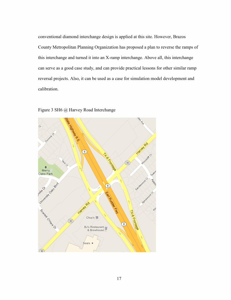
17

conventional diamond interchange design is applied at this site. However, Brazos

County Metropolitan Planning Organization has proposed a plan to reverse the ramps of

this interchange and turned it into an X-ramp interchange. Above all, this interchange

can serve as a good case study, and can provide practical lessons for other similar ramp

reversal projects. Also, it can be used as a case for simulation model development and

calibration.

Figure 3 SH6 @ Harvey Road Interchange

18

To investigate the interchange between Earl Rudder Freeway and Briarcrest Drive, the

following data needs to be gathered:

Geometry information of the interested interchange,

Signal timing plan of the diamond interchange,

Traffic flow volume around the interchange,

Vehicle speed on the freeway, frontage roads and crossing road,

Vehicle travel time on the frontage road.

3.3 Simulation Model Development

To build a simulation model in VISSIM for analysis, one has to code the following

components into the model:

Traffic Network Components

Scale

As mentioned before, the geometry design of the model will use the data from SH

6@Harvey rd interchange. So the snap shot taken form Google map will be used as

background in this model. Before starting to code the network accordingly, we have to

check the scale in order to represent real-world conditions. Figure 4 shows the

parameters for loading and modifying the background in VISSIM.

19

Figure 4 Background Settings in VISSIM

Links

Links in VISSIM represent freeway segments or road segments in actual world. Based

on the background image, all those frontage roads and cross streets are coded into the

model. In VISSIM, links can be defined with characteristics like number of lanes, lane

width, link length and link type etc. It also provides Display options for users to define

3D demonstration factors, which is very useful if visualization is needed. Link type can

impact vehicle behavior according to car-following and lane-changing theories.

20

Figure 5 Links in VISSIM

Connectors

All those links have to be connected by connectors, for they can’t connect with each

directly in VISSIM. So connectors serve as joints between links. It can define from

which lane connected to which lane. Plus, the “Route” option can define lane-changing

parameters. “Recalculate Spline” option can help generate smoother curves for

connection.

21

Figure 6 Connectors in VISSIM

Traffic in Network

Vehicle inputs

Vehicle inputs can be defined at each edge of the network in VISSIM. Vehicle inputs

parameters include traffic volume at each simulation time period, vehicle type, traffic

composition, desire speed distribution etc. Those vehicles generated from those inputs

will travel inside the network until meet the end of the network and disappear.

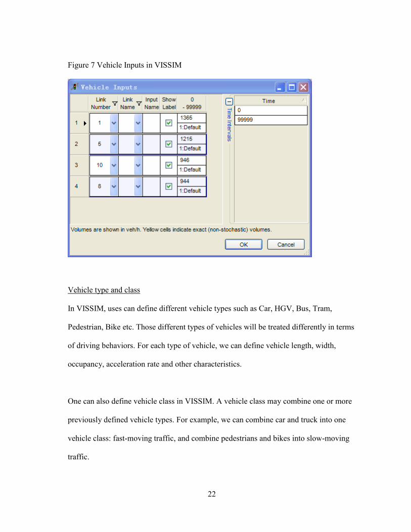
22

Figure 7 Vehicle Inputs in VISSIM

Vehicle type and class

In VISSIM, uses can define different vehicle types such as Car, HGV, Bus, Tram,

Pedestrian, Bike etc. Those different types of vehicles will be treated differently in terms

of driving behaviors. For each type of vehicle, we can define vehicle length, width,

occupancy, acceleration rate and other characteristics.

One can also define vehicle class in VISSIM. A vehicle class may combine one or more

previously defined vehicle types. For example, we can combine car and truck into one

vehicle class: fast-moving traffic, and combine pedestrians and bikes into slow-moving

traffic.

23

Figure 8 Vehicle Types in VISSIM

Routes

Routes in VISSIM are very essential parts in defining travelling path for each vehicle.

Figure 9 shows the right turn, through, and left turn movements routes in the model.

User can define associated turning percentage to each movement according to actual

data. Vehicles generated from inputs will split based on those turning ratio and move on

to their separated routes when they meet one of those route decision points.

24

Figure 9 Routes in VISSIM

Traffic Control

Signal Controllers

One common way of traffic control is signal control. In VISSIM, one can use different

types of signal controllers such as fixed time, NEMA, VAP etc. In this study, fixed time

signal controller is used. For signal controller, one can define its cycle length, offset and

green/red end etc. After defining those controller parameters, we have to build signal

heads for each lane at intersections. For those signal heads, one can define which signal

controller it’s using, which signal group it’s on (which phase), and the control type

(circular or arrow).

25

Figure 10 Signal Controllers in VISSIM

Priority Rule

Another traffic control approach is priority rule in VISSIM. Usually, priority control

approach is used at non-signalized intersections or at separating or joining links. In this

study, all intersections are signalized, but priority rule is still used to avoid confliction

when dealing with right turn movements and permitted left turn movements.

26

Figure 11 Priority Rule in VISSIM

Driving Behavior

VISSIM is a microscopic traffic simulation, which controls the driving behavior of

individual vehicles based on car-following and lane-changing models. Figure 12 shows

the driving behavior sets in VISSIM. There are five different types of driving behavior

categorized based on the link types (i.e. Urban, Right-side rule, Freeway, Footpath and

Cycle-Track). In this study, only Urban (motorized) type of driving behavior is used. All

those parameters in car-following and lane-changing model are adjustable. And they will

be adjusted in the calibration process to generate a simulation model closer to reality.

27

Figure 12 Driving Behavior Parameters in VISSIM

3.4 Simulation Model Calibration

Sensitivity Analysis

Too many parameters in VISSIM are adjustable, and it is a really intimidating work if

we take all those parameters into consideration. Thus, it is desirable to reduce the

amount of parameters needed to be calibrated. In this study, a sensitivity analysis is

conducted to find out those parameters that impose the most influence on simulation

model. This way, we can improve the efficiency of calibration.

28

Parameters that can be calibrated in VISSIM

A large number of parameters in VISSIM are adjustable, and those parameters are listed

in table 1. Some other parameters that are obviously indifferent are excluded, such as

lateral behavior and reaction to amber signals.

Table 1 Adjustable Parameters in VISSIM

Parameter Name Default Unit Change scale of

parameter

Car Following Model

Look ahead

distance

Max. 250 m 100~300

Observed vehicles 2 1~4

Wiedemann

99

Model

parameters

CC0 1.5 m 1~5

CC1 0.90 s 0.5~2.0

CC2 4.00 m 2~10

CC3 -8.00 -15~-3

CC4 -0.35 -0.7~-0.1

CC5 0.35 0.1~0.7

CC6 11.44 5~20

CC7 0.25 m/s2 0.1~1.0

CC8 3.50 m/s2 2.5~7

CC9 1.50 m/s2 0.5~ 6

29

Table 1 Continued

Parameter Name Default Unit Change scale of

parameter

Lane Changing Model

Own Maximum

deceleration

-4.00 m/s2 -5~-1

-1 m/s2 per distance 200 m 50~300

Accepted deceleration -1.00 m/s2 -1.50~-0.10

Trailing

vehicle

Maximum

deceleration

-3.00 m/s2 -5~-1

-1 m/s2 per distance 200 m 50~300

Accepted deceleration -0.50 m/s2 -1.50~-0.10

Waiting time before diffusion 60 s 20~60

Minimum headway 0.5 m 0.5~7.0

Route Emergency stop 5 m 5~10

Lane change 200 m 100~250

Desired

speed

distributio

n

Mean 60 km/h 60~90

Standard deviation 10 km/h 5~15

30

Paired t-test

In order to conduct sensitivity analysis, we change the value of parameters in table 1 and

conduct multi-runs. In this study, each time we increase the value of parameters 30% of

their default values. And for each parameter, we run the simulation with different

random seeds for 10 times. Average travel speed is used as the performance measure in

this study. Then we compare the results with changed parameters to the results with

default parameters using paired t-test. This way, sensitive parameters can be found.

The paired t-test is designed to handle correlation among matched pairs of measurements

or data points (Spiegelman, 2004). In this case, each time only the target parameter

varies and other elements remain the same, so the assumption of paired t-test applies.

Moreover, when the scatter plot of those two group outputs is plotted, a linear trend can

be found. Therefore, paired t-test is the best choice for comparison of default outputs and

changed outputs here.

Each time, we change one target parameter and run the simulation for 10 times. So for

24 parameters, altogether 240 runs are conducted. However, when we test whether the

sample space of 10 for each parameter is sufficient using formula , for most

parameters 10 times multi-run is not enough. Because of time limit, here we assume 10

times multi-run is good for all parameters. So paired t-test results are shown as follow:

31

Table 2 Paired t-test Results for Analysis of Sensitivity

Parameter Name Default

value

Changed

value

Average

output

change

(%)

P value

Car Following Model

Look ahead distance

Max. 250 325 1.56 0.23

Observed

vehicles 2 3 1.98 0.28

Wiedemann 99

CC0 1.5 1.95 4.71 0.00

CC1 0.9 1.17 3.08 0.23

CC2 4 5.2 5.56 0.00

CC3 -8 -10.4 0.24 0.84

CC4 -0.35 -0.455 0.42 0.75

CC5 0.35 0.455 0.23 0.86

CC6 11.44 14.872 1.46 0.50

CC7 0.25 0.325 1.17 0.40

CC8 3.5 4.55 0.11 0.93

CC9 1.5 1.95 2.59 0.03

32

Table 2 Continued

Lane Changing Model

Own

Maximum

deceleration -4 -5.2 2.48 0.23

1m/s^2 per

distance 200 260 1.37 0.18

Accepted


Trailing vehicle

Maximum


1m/s^2 per

distance 200 260 2.01 0.09

Accepted

deceleration -0.5 -0.65 1.87 0.10

Minimum headway 0.5 0.65 1.16 0.35

Route

Emergency

stop 5 6.5 1.49 0.06

Lane

change 200 260 2.67 0.08

Desired speed

distribution

Mean 60 78 7.72 0.00

Deviation 10 13 0.15 0.92

33

In statistics, those parameters with small p-values are significantly different, which

means they are sensitive parameters. In this study, if choose type I error (i.e. ) as 0.05,

four parameters can be found as having a significant impact on simulation model. But

none of those four parameters is related to lane-changing. So, we choose 0.10 as type I

error. This way, eight parameters are sensitive: CC0, CC2, CC9, Maximum deceleration

and reduction rate for trailing vehicle, emergency stop, lane change starting point and the

mean of desired speed distribution. In table 2, those eight sensitive parameters are

marked in red.

Initial Evaluation

This step is to test whether default parameters in the simulation model is sufficient to

represent field data. Simulation model with default parameters values is run for 10 times

and compared to field data.

34

Figure 13 Initial Evaluation Using Default Parameters

From figure 13, clearly the observed data is not within the range of simulated outcomes.

So default parameters can’t reasonably represent field conditions. Calibration is needed.

Calibrating Selected Parameters

The calibration process includes three parts. 1) Identify calibration parameters and their

acceptable ranges, 2) conduct statistical experimental design and generate reasonable

number of parameters sets, 3) conduct multi-run for each parameter set and find the most

feasible one.

Identification of calibration parameters

VISSIM provides so many adjustable parameters that it is almost impossible to calibrate

all of them. In this study, we only calibrate those sensitive parameters identified in the

35

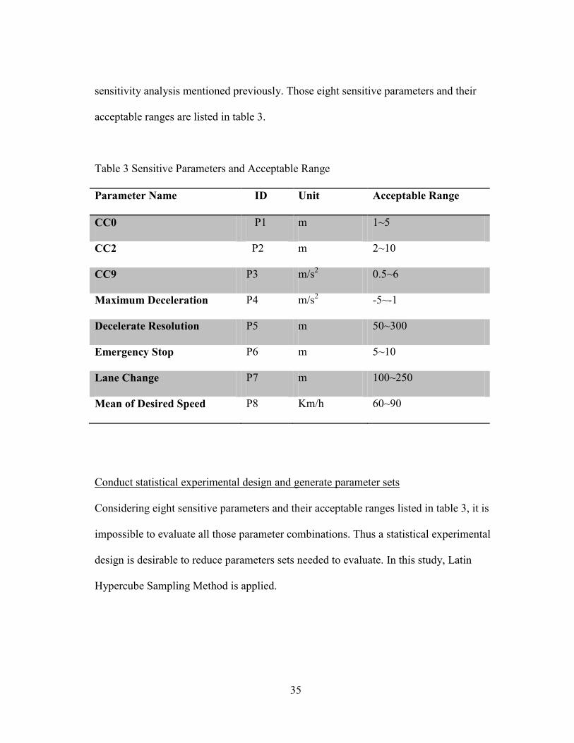
sensitivity analysis mentioned previously. Those eight sensitive parameters and their

acceptable ranges are listed in table 3.

Table 3 Sensitive Parameters and Acceptable Range

Parameter Name ID Unit Acceptable Range

CC0 P1 m 1~5

CC2 P2 m 2~10

CC9 P3 m/s2 0.5~6

Maximum Deceleration P4 m/s2 -5~-1

Decelerate Resolution P5 m 50~300

Emergency Stop P6 m 5~10

Lane Change P7 m 100~250

Mean of Desired Speed P8 Km/h 60~90

Conduct statistical experimental design and generate parameter sets

Considering eight sensitive parameters and their acceptable ranges listed in table 3, it is

impossible to evaluate all those parameter combinations. Thus a statistical experimental

design is desirable to reduce parameters sets needed to evaluate. In this study, Latin

Hypercube Sampling Method is applied.

36

Latin Hypercube Sampling Method is a space-filling design method that can spread the

points as evenly as possible around the operating space. This design should be used

when there is little or no information about the underlying effects of factors on responses.

LHS method is coded in JMP for use, and in this study, it generates 20 parameter sets for

feasibility test.

Table 4 Parameter Sets Generate by LHS Method

P1 P2 P3 P4 P5 P6 P7 P8

1 1.0 3.7 6.0 -2.9 50.0 10.0 147.4 85.3

2 1.4 10.0 4.8 -1.0 76.3 8.2 178.9 83.7

3 1.2 7.5 3.1 -2.3 155.3 6.6 100.0 61.6

4 3.1 5.4 5.7 -4.2 89.5 9.5 123.7 60.0

5 2.7 3.3 3.7 -3.9 168.4 9.2 210.5 82.1

6 3.7 9.6 1.1 -2.7 207.9 8.9 242.1 69.5

7 2.1 7.1 2.2 -3.5 63.2 9.7 218.4 78.9

8 4.4 6.2 2.5 -1.4 102.6 7.6 234.2 86.8

9 1.8 2.8 1.4 -1.6 221.1 7.1 155.3 72.6

10 2.5 7.9 1.9 -1.2 115.8 8.7 186.8 75.8

11 3.5 4.1 4.6 -4.8 234.2 6.3 163.2 74.2

12 4.2 9.2 5.1 -4.4 128.9 7.9 194.7 77.4

13 1.6 5.8 4.0 -4.6 247.4 7.4 115.8 63.2

14 3.9 4.9 4.3 -2.5 286.8 5.3 131.6 71.1

37

Table 4 Continued

P1 P2 P3 P4 P5 P6 P7 P8

15 2.3 2.4 5.4 -3.3 142.1 6.1 107.9 80.5

16 3.3 8.7 2.8 -2.1 181.6 5.8 139.5 67.9

17 2.9 6.6 0.8 -1.8 260.5 5.5 226.3 90.0

18 4.8 4.5 3.4 -3.7 194.7 8.4 250.0 88.4

19 4.6 2.0 1.7 -5.0 273.7 6.8 171.1 66.3

20 5.0 8.3 0.5 -3.1 300.0 5.0 202.6 64.7

Determine the most feasible parameter set

For each parameter set, 5 times multi-run was conducted. The parameter set that

generate the least discrepancy between simulated data and observed data is chosen as the

most feasible parameter set and will be used in the simulation model. The optimal

parameter set generated is shown in table 5:

Table 5 Calibrated Parameters Using GA

P1 P2 P3 P4 P5 P6 P7 P8

Default 1.5 4 1.5 -3 200 5 200 60

Calibrated 3.9 4.9 4.3 -2.5 287 5.3 132 71

After calibration, the model developed in VISSIM will be ready for analysis.

38

CHAPTER IV

SIGNAL TIMING OPTIMIZATION

There are two reasons to optimize the signal timing strategies. First, optimized signal

timing strategies can show the actual potential of each interchange design, and the

researcher can focus on how traffic flow operates under different interchange designs by

excluding the influence of signal timing. Second, this process can provide

recommendations of the optimal timing strategies for those two interchange designs,

especially the X-ramp interchange design.

To find the optimal signal timing for each scenario, the software package Synchro is

used in the following procedures:

Examine the two popular interchange timing strategies (TTI 4-phase and three-phase

operation), and select the one that yields less delay

Optimize cycle length

Optimize green splits

Left turn treatment, whether permitted left turn is allowed.

After all those procedures, an optimal signal timing plan can be generated for each

scenario. The following is the procedures for signal timing optimization using Synchro.

39

4.1 Optimization Tool – Synchro

Synchro is a macroscopic analysis and optimization software in traffic engineering. It is

very helpful in dealing with signal timing optimization problems. Synchro mainly

utilizes the Highway Capacity Manual (HCM) methodology for signalized intersections.

It can provide optimal solutions to some complicated situations such as three phase and

four phase operation at a diamond interchange.

4.2 Signal Timing Strategies

Typically, there are two signal timing strategies recommended for diamond interchanges:

Three-Phase Operation and Four-Phase Operation.

Three-Phase Operation

Figure 14 shows the three-phase timing plan for a diamond interchange and the

numbering strategy for intersection movements. The figure shown is just a basic three-

phase strategy with no overlapping, but three-phase operation can have overlaps. Also,

this is a lead-lead situation, which means left turn movements phase is leading or before

the through movements phase. Lag-lag situation is another option.

40

Figure 14 Three-Phase Operations

Four-Phase Operation

Figure 15 shows the four-phase timing plan for a diamond interchange and the

numbering strategy for intersection movements. The major benefit of the four-phase

operation is that, if properly timed, hardly any movement has to stop inside the

intersection. This is a huge advantage especially for those tight diamonds where the left

side intersection and right side intersection are too close together that queue storage is a

problem. However, four-phase operation has its disadvantage. Comparing to three-phase,

four-phase has one more phase each cycle, which means more lost time for each cycle.

Thus, four-phase operation typically associates with less capacity.

41

Figure 15 Four-Phase Operations

Both the three-phase and four-phase operation strategies have been coded into Synchro

as signal timing examples, so we only have to modify some parameters (such as traffic

volumes, road length, etc.) and they can be ready for analysis.

4.3 Cycle Length Optimization

According to Webster, the relationship between delay and cycle length is a convex

function. When cycle length increases, the general delay during each cycle increases, on

the other hand, when cycle length decreases, the lost time percentage increases, and the

capacity of this intersection drops. Therefore, there exists an optimal cycle length that

can generate minimum delay for a specific intersection. With the help of Synchro, the

optimization of cycle length is pretty simple. After modifying associated parameters

42

both in four-phase operation scenario and three-phase operation scenario, by pushing the

Optimize button for cycle length, Synchro will automatically calculate the delay and

generate the optimal cycle length for you.

4.4 Phase Split Optimization

The method Synchro uses to optimize phase split is based on the equal degree saturation

approach. This approach will allocate green time to each critical movement in proportion

to its percentage. Critical movements are those with the highest volume to saturation

flow ratio per phase. To optimize phase split in Synchro is simple too, just click the

Optimize button near the phase split option. The results may have overlap situation if

necessary.

4.5 Left Turn Treatment

The left turn treatment options can be protected only, protected plus permitted, or

permitted only. In Synchro, it is not very hard to set those three left turn treatment

options and not hard to evaluate either. Also, it provides those three options for each left

turn movements, so we can set different treatment for different left turn movements. In

most scenarios of this study, permitted only is not a good option because of the heavy

opposing through traffic. Also, for the same reason, protected plus permitted has very

limited advantage over protect only option.

43

4.6 Case Study Example

To illustrate the above procedure, the case study of SH6 @ Harvey Road interchange is

selected as a signal timing optimization example. Figure 16 shows the model in Synchro

with all those traffic volume inputs. And to optimize the signal timing plan, the

following procedure is used in the software package Synchro:

Examine the two popular interchange timing strategies (TTI four-phase and three-

phase operation)

Optimize cycle length

Optimize green splits

Left turn treatment.

Figure 16 Network Information in Synchro

44

By following the optimization procedure, all the delays calculated after each step is

shown in the table below:

Table 6 Summary of the Optimization Procedure

Optimizing Step Four-Phase Three-Phase

Setting Strategies 43.2 39.4

Cycle Length 36.9 24.1

Green Split 36.9 24.1

Left Turn Treatment 35.7 23.6

Therefore, by comparing the final results, we can find that the optimized Three-Phase

Operation can generate less delay. Figure 17 is the optimized signal timing plan for the

interchange.

Figure 17 Signal Timing Plan for the SH6 @ Harvey Rd Interchange

45

CHAPTER V

MODEL ANALYSIS

5.1 Experimental Design

Varying Factors in Experimental Design

To explicitly investigate the advantage and disadvantage of ramp reversal, as well as the

impact of traffic demand pattern on interchange operations, a thorough simulation

analysis is needed. Thus, different scenarios will be created based on this purpose. Since

interchanges normally are symmetric, in this study, only one side will be investigated

and the other side is assumed to be the same condition to simplify the analysis.

Following five major factors will be changed when designing different scenarios:

1) Interchange design. In order to study the best suitable interchange design under

different situations, the researcher plan to carry out ramp reversal based on the

initial diamond interchange.

2) Demand patterns. In order to examine the impact of traffic demand pattern on

interchange operations, different OD patterns need to be designed. What actually

matters is the exiting demand around the interchange. So in this study, the attraction

area’s location is changing from downstream the intersection to upstream the

intersection.

3) Demand level. The demand level here is mainly in reference to the attraction or the

exiting volume from the freeway.

46

4) Flow on frontage road intersection (the flow resulting from exiting demand is not

included). To measure the operation of frontage road and crossing street intersection,

the sum of degree of saturation of all critical lane groups is used. By changing the

saturation rate of the signalized intersection, the researcher can analyze the impact

of the flow on frontage road and crossing street.

5) Turning movements’ percentage of critical movements.

As shown in figure 18, movements 4 and 8 are essential in this study and their hourly

volume during peak period would be a changing factor. Also, the percentage of turning

movements of phase 4 and 8 would be a varying factor. The relative ratio of all the other

movements would be held constant to simplify our problem.

Figure 18 Diamond Interchange Movement/Phase

Thus the varying factors that will be used in experimental design and their range

(minimum value to maximum value) are summed up in table 7:

47

Table 7 Factors in Experimental Design

Factors Measurement Varying Range

Minimum Maximum

Demand at the

intersection

0.4 1.0

Peak hour volume

for phase 4 and 8

Veh/hr/ln 200 600

Percentage of the

through

movement for

phase 4 and 8

% 20 80

Latin Hypercube Design

A space-filling design algorithm – Latin Hypercube Design is selected for this study to

generate design points to bind the bias in this experiment. Latin Hypercube Design (SAS

Institute Inc. 2007) chooses points to maximize the minimum distance between design

points but with a constraint. The constraint maintains the even spacing between factor

levels. Since LHD can’t handle categorical factors, three continuous factors in table 7

and their varying ranges are input to statistical software JMP. The following table

summarizes all the design points considering only continuous factors:

48

Table 8 Latin Hypercube Design

Scenarios Volume

Through

Percentage

1 600 0.72 26

2 453 0.75 39

3 474 0.56 23

4 558 0.53 42

5 347 0.94 33

6 305 0.87 80

7 495 0.84 77

8 389 0.59 74

9 263 0.62 45

10 579 0.81 55

11 284 0.40 64

12 368 0.78 58

13 200 0.91 52

14 537 0.49 67

15 432 0.43 48

16 242 0.68 20

17 221 0.65 71

18 326 0.46 29

19 516 0.97 36

20 411 1.00 61

Simulation Scenarios

Since Latin Hypercube Design can’t deal with categorical factors, table 8 didn’t include

interchange type factor into consideration. However, this factor is essential in our study

49

and can’t be ignored. Thus, this categorical factor has to be crossed with the design

generated from the previous step. Also, we need to be careful when constructing those

scenarios, especially when dealing with the traffic volume on frontage road at X-ramp

interchange. Because in X-ramp situations, most of the traffic will have to remain on the

freeway until meet the exit ramp downstream. So the traffic volume will be greatly

reduced at the frontage road.

In this study, first of all, we assume 50% of the original traffic will remain on the

frontage road after the ramp reversal. Scenarios 21 to 40 are constructed based on this.

Then, we assume the 90% of the original traffic are from the upstream exit ramp in the

diamond interchange design for simplification. Therefore, all those traffic volume on

frontage road in scenarios 41 to 60 will only be 10% of what it used to be. Table 9

summarizes the new 60 scenarios that will be used in simulation analysis.

Table 9 Simulation Scenarios Summary

Scenarios Type Volume V/C Percentage

1 1 600 0.72 26

2 1 453 0.75 39

3 1 474 0.56 23

4 1 558 0.53 42

5 1 347 0.94 33

6 1 305 0.87 80

7 1 495 0.84 77

8 1 389 0.59 74

50

Table 9 Continued


9 1 263 0.62 45

10 1 579 0.81 55

11 1 284 0.40 64

12 1 368 0.78 58

13 1 200 0.91 52

14 1 537 0.49 67

15 1 432 0.43 48

16 1 242 0.68 20

17 1 221 0.65 71

18 1 326 0.46 29

19 1 516 0.97 36

20 1 411 1.00 61

21 2 300 0.72 26

22 2 226 0.75 39

23 2 237 0.56 23

24 2 279 0.53 42

25 2 174 0.94 33

26 2 153 0.87 80

27 2 247 0.84 77

28 2 195 0.59 74

29 2 132 0.62 45

30 2 289 0.81 55

31 2 142 0.40 64

32 2 184 0.78 58

33 2 100 0.91 52

34 2 268 0.49 67

51

Table 9 Continued


35 2 216 0.43 48

36 2 121 0.68 20

37 2 111 0.65 71

38 2 163 0.46 29

39 2 258 0.97 36

40 2 205 1.00 61

41 2 60 0.72 26

42 2 45 0.75 39

43 2 47 0.56 23

44 2 56 0.53 42

45 2 35 0.94 33

46 2 31 0.87 80

47 2 49 0.84 77

48 2 39 0.59 74

49 2 26 0.62 45

50 2 58 0.81 55

51 2 28 0.40 64

52 2 37 0.78 58

53 2 20 0.91 52

54 2 54 0.49 67

55 2 43 0.43 48

56 2 24 0.68 20

57 2 22 0.65 71

58 2 33 0.46 29

59 2 52 0.97 36

60 2 41 1.00 61

52

* In table 9, Type 1 indicates Diamond Interchange;

Type 2 indicates X-ramp Interchange.

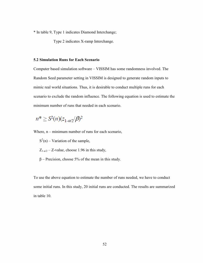
5.2 Simulation Runs for Each Scenario

Computer based simulation software – VISSIM has some randomness involved. The

Random Seed parameter setting in VISSIM is designed to generate random inputs to

mimic real world situations. Thus, it is desirable to conduct multiple runs for each

scenario to exclude the random influence. The following equation is used to estimate the

minimum number of runs that needed in each scenario.

Where, n – minimum number of runs for each scenario,

S2(n) – Variation of the sample,

Z1-a/2 – Z-value, choose 1.96 in this study,

β – Precision, choose 5% of the mean in this study.

To use the above equation to estimate the number of runs needed, we have to conduct

some initial runs. In this study, 20 initial runs are conducted. The results are summarized

in table 10.

53

Table 10 Summary of Initial Runs

Seed Delay Seed Delay

1 24.65 11 25.05

2 24.57 12 24.68

3 24.79 13 24.97

4 25.30 14 25.04

5 24.95 15 25.20

6 25.36 16 24.86

7 25.23 17 24.92

8 25.89 18 24.56

9 24.69 19 25.48

10 25.58 20 25.39

Average 25.06

SDV 0.37

Based on the average and standard deviation of those initial runs, we can estimate that

the minimum number of simulation runs for each scenario is 9.

5.3 Additional Factors

To consider the full impact of ramp reversal, there are two other traffic groups needing

to be taken into account. First, travelers with cross street destinations will need to get off

freeway from the upstream interchange after ramp reversal. This is the negative impact

resulting from ramp reversal. Second, travelers with downstream destinations will

remain on freeway until after the intersection. This is the positive impact resulting from

ramp reversal.

54

We didn’t include those two factors in the experimental design because they only will

make the situation much more complicated. With the time constraint, we can’t conduct

more simulation runs to consider those two traffic groups. Thus, a better way to go

around is to make some assumptions and separate them from the simulation scenarios.

For those travelers remaining on freeway, they benefit by avoiding one signal. So the

benefit of those travelers can be assumed to be the average control delay at the

intersection. For those travelers getting off the freeway early, the cost can be assumed to

be the difference of freeway travel time and frontage road travel time plus the right-turn

delay at the intersection. The right-turn delay can be approximated by assuming those

vehicles will experience the same delay as the average right-turn delay in simulation

model.

5.4 Simulation Results

Signal Timing Optimization Results

There are two reasons to optimize the signal timing strategies. First, optimized signal

timing strategies can show the actual potential of each interchange design, and the

researcher can focus on how traffic flow operates under different interchange designs by

excluding the influence of signal timing. Second, this process can provide

recommendations of the optimal timing strategies for those two interchange designs,

especially the X-ramp interchange design.

55

So before we analyze those 60 scenarios in VISSIM, we have to find the optimal signal

timing plan for each scenario. The procedure of finding the optimal signal timing plan is

explained explicitly in chapter 4. The following table summarizes the strategy that will

be used for each scenario.

Table 11 Summary of Signal Timing Strategies

Scenarios Signal Scenarios Signal Scenarios Signal

1 4p 21 3p 41 3p

2 3p 22 3p 42 3p

3 3p 23 3p 43 3p

4 4p 24 3p 44 3p

5 3p 25 3p 45 3p

6 3p 26 3p 46 3p

7 4p 27 4p 47 3p

8 4p 28 4p 48 3p

9 3p 29 3p 49 3p

10 3p 30 3p 50 3p

11 4p 31 4p 51 4p

12 3p 32 3p 52 3p

13 3p 33 3p 53 3p

14 4p 34 3p 54 3p

15 4p 35 4p 55 4p

16 3p 36 3p 56 3p

17 4p 37 3p 57 3p

18 3p 38 4p 58 4p

19 4p 39 3p 59 3p

20 3p 40 3p 60 3p

56

* In table 11, Signal 4p indicates Four-Phase Operation,

Signal 3p indicates Three-Phase Operation.

In table 11, we can find that for most cases, Three-Phase Operation is a better strategy.

Only 17 scenarios out of those 60 scenarios will better off with Four-Phase Operation.

Among those 17 scenarios, we can group them into two categories according to the

reason why four-phase is suitable for them.

The first group includes scenarios 4, 11, 14, 15, 31, 35, 38, 51, 55, 58. Those scenarios

share one thing in common. That is they all have very low degree of saturation (below

0.6). This means four-phase operation is more suitable for intersections with lower

degree of saturation. This is because four-phase operation can provide smoother traffic

movement inside the interchange and thus generate less overall delays, but with one

more phase each cycle comparing to three-phase operation, it will have one more lost

time each cycle thus when traffic demand increases at the interchange, the delay will

increase significantly.

The second group includes scenarios 1, 7, 8, 17, 19, 27, 28. Those scenarios all have

very high turning movements at the frontage road (above 65%). This could mean that

four-phase operation also works well when the turning movements (especially left turns)

are high. This is mainly because four-phase operation can provide a smoother movement

and hardly any vehicle needs to stop inside the intersections if properly timed.

57

VISSIM Results

To investigate the difference between diamond interchange and X-ramp interchange, 60

scenarios are studied using simulation software – VISSIM. Each scenario is run for 9

times with different random seed. Table below summarizes the simulation study:

Table 12 Summary of VISSIM Results

Scenarios Type Volume V/C Percentage Signal Delay

1 1 600 0.72 26 4p 51.8

2 1 453 0.75 39 3p 23.5

3 1 474 0.56 23 3p 23.7

4 1 558 0.53 42 4p 23.3

5 1 347 0.94 33 3p 24.5

6 1 305 0.87 80 3p 29.0

7 1 495 0.84 77 4p 29.6

8 1 389 0.59 74 4p 23.8

9 1 263 0.62 45 3p 21.4

10 1 579 0.81 55 3p 25.1

11 1 284 0.40 64 4p 21.0

12 1 368 0.78 58 3p 24.9

13 1 200 0.91 52 3p 24.3

14 1 537 0.49 67 4p 26.1

15 1 432 0.43 48 4p 22.0

16 1 242 0.68 20 3p 21.4

17 1 221 0.65 71 4p 23.1

18 1 326 0.46 29 3p 20.2

58

Table 12 Continued


19 1 516 0.97 36 4p 30.6

20 1 411 1.00 61 3p 26.7

21 2 300 0.72 26 3p 43.9

22 2 226 0.75 39 3p 23.4

23 2 237 0.56 23 3p 22.9

24 2 279 0.53 42 3p 23.1

25 2 174 0.94 33 3p 26.2

26 2 153 0.87 80 3p 24.5

27 2 247 0.84 77 4p 25.3

28 2 195 0.59 74 4p 23.7

29 2 132 0.62 45 3p 26.3

30 2 289 0.81 55 3p 22.7

31 2 142 0.40 64 4p 23.6

32 2 184 0.78 58 3p 24.8

33 2 100 0.91 52 3p 26.2

34 2 268 0.49 67 3p 23.2

35 2 216 0.43 48 4p 24.1

36 2 121 0.68 20 3p 24.3

37 2 111 0.65 71 3p 23.6

38 2 163 0.46 29 4p 23.1

39 2 258 0.97 36 3p 25.8

40 2 205 1.00 61 3p 25.1

41 2 60 0.72 26 3p 41.9

42 2 45 0.75 39 3p 22.7

43 2 47 0.56 23 3p 21.6

44 2 56 0.53 42 3p 21.4

59

Table 12 Continued


45 2 35 0.94 33 3p 25.0

46 2 31 0.87 80 3p 23.8

47 2 49 0.84 77 3p 23.8

48 2 39 0.59 74 3p 21.7

49 2 26 0.62 45 3p 22.3

50 2 58 0.81 55 3p 20.6

51 2 28 0.40 64 4p 21.4

52 2 37 0.78 58 3p 23.0

53 2 20 0.91 52 3p 24.4

54 2 54 0.49 67 3p 21.1

55 2 43 0.43 48 4p 21.6

56 2 24 0.68 20 3p 22.1

57 2 22 0.65 71 3p 21.9

58 2 33 0.46 29 4p 20.9

59 2 52 0.97 36 3p 24.6

60 2 41 1.00 61 3p 24.1

* In table 12, Type 1 indicates Diamond Interchange;

Type 2 indicates X-ramp Interchange.

Signal 4p indicates Four-Phase Operation,


Besides those four factors considered in the simulation study, we have another two

groups of traffic left out for the reason of simplifying our experiment. Now we have to

60

include those two groups of traffic. First, travelers with cross street destinations will

need to get off freeway from the upstream interchange after ramp reversal. This is the

negative impact resulting from ramp reversal. Second, travelers with downstream

destinations will remain on freeway until after the intersection. This is the positive

impact resulting from ramp reversal.

For those travelers remaining on freeway, they benefit by avoiding one signal. So the

benefit of those travelers can be assumed to be the average control delay at the

intersection. For those travelers getting off the freeway early, the cost can be assumed to

be the difference of freeway travel time and frontage road travel time plus right-turn

delay at the intersection. The right-turn delay can be approximated by assuming those

vehicles will experience the same delay as the average right-turn delay in simulation

model.

But this is assuming that those travelers won’t have to go through the upstream

intersection, which means that the upstream interchange have to be X-ramp interchange.

The table below summarizes the revised delay for X-ramp design after considering those

two groups of traffic.

61

Table 13 Revised Results for X-ramp Interchange


21 2 300 0.72 26 3p 48.3

22 2 226 0.75 39 3p 26.3

23 2 237 0.56 23 3p 27.9

24 2 279 0.53 42 3p 27.6

25 2 174 0.94 33 3p 28.3

26 2 153 0.87 80 3p 25.1

27 2 247 0.84 77 4p 26.3

28 2 195 0.59 74 4p 25.1

29 2 132 0.62 45 3p 28.4

30 2 289 0.81 55 3p 25.0

31 2 142 0.40 64 4p 25.8

32 2 184 0.78 58 3p 26.4

33 2 100 0.91 52 3p 27.2

34 2 268 0.49 67 3p 25.8

35 2 216 0.43 48 4p 28.2

36 2 121 0.68 20 3p 26.9

37 2 111 0.65 71 3p 24.5

38 2 163 0.46 29 4p 27.3

39 2 258 0.97 36 3p 28.4

40 2 205 1.00 61 3p 26.4

41 2 60 0.72 26 3p 49.8

42 2 45 0.75 39 3p 27.9

43 2 47 0.56 23 3p 30.6

44 2 56 0.53 42 3p 29.4

45 2 35 0.94 33 3p 28.8

46 2 31 0.87 80 3p 24.9

62

Table 13 Continued


47 2 49 0.84 77 3p 25.7

48 2 39 0.59 74 3p 24.2

49 2 26 0.62 45 3p 26.0

50 2 58 0.81 55 3p 24.8

51 2 28 0.40 64 4p 25.4

52 2 37 0.78 58 3p 26.0

53 2 20 0.91 52 3p 26.2

54 2 54 0.49 67 3p 25.8

55 2 43 0.43 48 4p 28.9

56 2 24 0.68 20 3p 26.7

57 2 22 0.65 71 3p 23.6

58 2 33 0.46 29 4p 28.5

59 2 52 0.97 36 3p 29.2

60 2 41 1.00 61 3p 26.4

* In table 13, Type 2 indicates X-ramp Interchange.

Signal 4p indicates Four-Phase Operation,


Paired t-Test

Paired t-test is utilized here to compare those simulation results. Given two paired

simulation results Xi and Yi of n values, the paired t-test determines whether they differ

from each other in a significant way under the assumption that the paired differences are

independent and identically normally distributed.

63

To apply the test, let

Then define t by

N is 9 in this study, and once t is found using the equations above, a p-value can be

found using a table of values from student’s t distribution. The confidence interval is

selected as 90%. So if the p-value is below the threshold value for 90% CI, we can reject

the null hypothesis and conclude that there is a significant difference between those two

pairs.

By comparing those results using paired t-test, we can find that the following factors are

essential when comparing diamond interchange with X-ramp interchange:

Interchange Density

Interchange density is the number of interchanges per mile. This is an important role

because distance between two interchanges will be essential when calculating the delay

caused by those vehicles getting off freeway early in order to reach the cross street

destinations. In table 13, the results are calculating using the distance of 800 meters,

which is the distance between two interchanges in the case study. After experimenting

with some more numbers, we find that, for most cases, a distance more than one mile

64

would cause too much delay, so ramp reversal is not beneficial when interchange density

is low.

Upstream Interchange Design

This factor also will impact those vehicles with cross street destinations. If the upstream

interchange type is diamond, those travelers have to take the exit ramp before upstream

interchange intersection. So they will have to experience the control delay on the

upstream intersection. On the other hand, if upstream interchange is X-ramp interchange,

it will not increase overall delay. So X-ramp interchange is more desirable when

upstream interchange type is also X-ramp design.

Traffic Volume on Frontage Road

By comparing scenarios 1, 7, 10, 14, 19 with 21, 27, 30, 34, 39 and 41, 47, 50, 54, 59,

we can find that when traffic volume on frontage road is high, X-ramp interchange is

better than Diamond interchange. The p value of this comparison is shown in table 14,

and all those p values are smaller than 0.10 and indicate significant difference between

comparison groups. This is because of two reasons. First, X-ramp interchange can

redirect those vehicles through the freeway to the downstream exit ramp so that the

demand on the intersections will be relieved. Second, those redirected traffic can also

benefit from avoiding the intersection. Of course, this factor should be considered

together with the movement percentage factor to have a better appreciation of scheme.

65

From the simulation results, ramp reversal is recommended when the traffic volume on

frontage road is around 500 vehicles per hour per lane.

Table 14 Comparison Results 1

Comparison Scenarios Pairs P-value

Scenario 1 Scenario 21 < 0.01

Scenario 7 Scenario 27 0.03




Scenario 1 Scenario 41 < 0.01





Through Movement Percentage on Frontage Road

Scenarios 6, 7, 14 and 26, 27, 34 and 46, 47, 54 clearly demonstrate the impact of

through movement percentage. The p value of this comparison is shown in table 15, and

all those p values are smaller than 0.10 and indicate significant difference between

comparison groups. Basically, when through movement percentage is high, X-ramp

interchange design is better. High through movement percentage means that more

travelers’ destinations are located downstream. As mentioned before, this factor should

be considered together with the traffic volume factor. When both of them are high,

which really means the downstream attraction is large; X-ramp interchange design is

66

desirable. Ramp reversal is recommended when the through movement percentage is

higher than 65.









Intersection Saturation Rate

Looking at scenarios 7, 10, 19 and 27, 30, 39 and 47, 50, 59, we can find that

intersection saturation rate also plays an important role in determining whether a ramp

reversal is needed. The p value of this comparison is shown in table 16, and all those p

values are smaller than 0.10 and indicate significant difference between comparison

groups. When the demand at the intersection is high (above 0.8 is recommended), ramp

reversal will be beneficial because it can help keep many travelers remain on freeway

and exit downstream to avoid going through the intersection.

67









68

CHAPTER VI

CONCLUSION AND RECOMMENDATIONS

6.1 Signal Timing Strategy Conclusions

To better explore the full potential of diamond interchange and X-ramp interchange,

signal timing optimization has been conducted with the help of Synchro. After

optimizing all those 60 scenarios, we conclude that for most cases, Three-Phase

Operation is better than Four-Phase Operation, except for the following two situations:

Degree of saturation is low (below 0.6). This means four-phase operation is more

suitable for intersections with lower degree of saturation. This is because four-phase

operation can provide smoother traffic movement inside the interchange and thus

generate less overall delays, but with one more phase each cycle comparing to three-

phase operation, it will have one more lost time each cycle thus when traffic demand

increases at the interchange, the delay will increase significantly.

Turning movements at the frontage road is high (above 65%). This could mean that

four-phase operation also works well when the turning movements (especially left

turns) are high. This is mainly because four-phase operation can provide a smoother

movement and hardly any vehicle needs to stop inside the intersections if properly

timed.

69

6.2 Ramp Reversal Conclusions

To investigate the benefit of ramp reversal, 60 scenarios have been run in VISSIM. And

we conclude that the following factors need to be considered when comparing diamond

interchange and X-ramp interchange:

1) Interchange density. The distance between two interchanges will play an important

role when calculating the delay caused by those vehicles getting off freeway early in

order to reach the cross street destinations. For most cases, a distance more than one

mile would cause too much delay, so ramp reversal is not beneficial when

interchange frequency is low.

2) Upstream interchange design. This factor also will impact those vehicles with cross

street destinations. If the upstream interchange type is diamond, those travelers have

to take the exit ramp before upstream interchange intersection. So they will have to

experience the control delay on the upstream intersection. On the other hand, if

upstream interchange is X-ramp interchange, it will not increase overall delay. So

X-ramp interchange is more desirable when upstream interchange type is also X-

ramp design.

3) Traffic volume on frontage road. This factor needs to be considered together with

the movement percentage factor. But basically, when traffic volume on frontage

road is high, a ramp reversal is beneficial. According to the simulation data, ramp

reversal is recommended when the traffic volume on frontage road is around 500

vehicles per hour per lane.

70

4) Through movement percentage on frontage road. When through movement demand

is high, which means more travelers’ destinations are located downstream, X-ramp

interchange design will be desirable. Ramp reversal is recommended when the

through movement percentage is higher than 65.

5) Intersection saturation rate. When the demand at the intersection is high, ramp

reversal will be beneficial because it can help keep many travelers remain on

freeway and exit downstream to avoid going through the intersection. A saturation

rate greater than 0.8 is recommended when considering ramp reversal.

6.3 Future Research Recommendations

This study has conducted a thorough investigation on comparing diamond interchange

design with X-ramp interchange design, especially focused on the impact of traffic

demand pattern and demand level. However, future research may still be needed in

following aspects:

Investigate more advanced signal timing strategies for interchanges, such as

actuated signal timing,

Focus more on the geometric factors’ impact on ramp reversal,

Consider more detailed and practical situations and develop a guideline for ramp

reversal.

71

REFERENCES

Araujo, J. J., Setti, L. R., Analysis of Heavy-vehicle Impacts on a Bridge Using

Microsimulation. In Transporte em Transformacao XII, pp. 23-42. 2008

Bonneson, J.A., S. Lee, Actuated Controller Settings for the Diamond Interchanges with

Three-Phase Operation. Report Number: TTI/ITS RCE-01/01, Texas Transportation

Institute, Texas A&M University, College Station, TX, Sep 2000.

Borchardt, D. and E. Chang. Alternative Analysis of X-Ramp and Diamond Ramp

Designs, Research Report 335-1F, Texas Transportation Institute, Texas A&M

University, College Station, TX, October 1986.

Chelewicki, Gilbert (2003). New Interchange and Intersection Designs: The

Synchronized Split-Phasing Intersection and the Diverging Diamond Interchange. 2nd

Urban Street Symposium (Anaheim, California), July 28-30, 2003.

Cooner, S.A., S. Venglar, Y. Rathod, E.J. Pultorak, J.C. Williams, P. Vo, and S.P.

Mattingly, Ramp Reversal Projects: Guidelines for Successful Implementation. Report

No. FHWA/TX-07/0-5105-1, Texas Transportation Institute, Texas A&M University,

College Station, TX, July 2007.

72

Engelbrecht, R.J. Advanced Traffic Signal Control for Diamond Interchanges.

Transportation Research Record: Journal of the Transportation Research Board, Issue

1856, 2003, p. 231-238

Elefteriadou, L., C. Fang, R. Roess, and E. Prassas, Methodology for Evaluating the

Operational Performance of Interchange Ramp Terminals. Transportation Research

Record: Journal of the Transportation Research Board, Issue 1920, 2005, pp 13-24.

Garber, N.J. and M.D. Fontaine, Guidelines for Preliminary Selection of the Optimum

Interchange Type for a Specific Loaction. Virginia Transportation Research Council,

FHWA/VTRC 99-R15, 1999, 120 p.

Gattis, J.L., C.J. Messer, and V.G. Stover. Delay to Frontage Road Vehicles at

Intersections with Ramps. Report No. FHWA/TX-86/402-2, Texas Transportation

Institute, Texas A&M University, College Station, TX, June 1988.

Goldberg, D. E., Generic Algorithm in Search Optimization and Machine Learning.

Addison-Wesley Publishing Co., Reading Mass. 1989.

Irvine, Y.D., D.B. Fambro, Implementation Guidelines for Retiming Diamond

Interchanges. Report Number: 1164-3, Texas Transportation Institute, Texas A&M

University, College Station, TX, Dec 1992.

73

Lee, S. Messer, C.J., J. Carroll, C. Keechoo, Actuated Signal Operations of Congested

Diamond Interchanges. Journal of Transportation Engineering, Oct2006, Vol. 132 Issue

10, p. 790-799.

Lee, S., C.J. Messer, J. Carroll, Evaluation of Actuated Control of Diamond

Interchanges with Advanced Experimental Design. Journal of Advanced Transportation.

Mar2003, Vol. 37 Issue 2, p. 195-210.

Liu, C., Hammad, A., Itoh, Y., Maintenance Strategy Optimization of Bridge Decks

Using Genetic Algorithm. J. Transp. Engg. 123, 91-100, 1997

Messer, C.J. and D.J. Berry. Effects of Design Alternatives on Quality of Service at

Signalized Diamond Interchanges. Transportation Research Record: Journal of the

Transportation Research Board, Issue 538, 1975, p. 20-31.

Messer, C.J., D.B. Fambro and S.H. Richards, Optimization of Pretimed Signalized

Diamond Interchanges, Transportation Research Record: Journal of the Transportation

Research Board, Issue 644, 1977, p. 78-84.

74

Nowlin, R.L., and K. Fitzpatrick. Two-sided Weaving Analysis on One-Way Frontage

Roads, Report 1393-2, Texas Transportation Institute, Texas A&M University, College

Station, TX, August 1996.

Park, B. and Qi, H. Development and Evaluation of a Procedure for the Calibration of

Simulation Models. Transportation Research Record: Journal of the Transportation

Research Board, No, 1934, Transportation Research Board of the National Academies,

Washington, D.C., 2005, pp. 208-217.

Park, B., and J. D. Schneeberger. Microscopic Simulation Model Calibration and

Validation: A Case Study of VISSIM for a Coordinated Actuated Signal System. In

Transportation Research Board, No. 1856, Transportation Research Board of the

National Academies, Washington, D. C., 2003, pp. 185-192.

SAS Institute Inc. 2007. <JMP Design of Experiments>. Cary, NC: SAS Institute Inc.

Teklu, F., Sumalee, A., A Genetic Algorithm Approach for Optimizing Traffic Control

Signals Considering Routing. Computer-Aided Civil and Infrastructure Engineering 22,

31-43, 2007

VISSIM User Manual, Version 4.0, PTV Planug Transport Verkehr AG, Innovative

Transportation Concepts, Inc., 2004.

Investigation of the Implementation of Ramp Reversal at A ...

Documents

Transcript of Investigation of the Implementation of Ramp Reversal at A ...