INVESTIGATION OF THE CORRELATIONS FOR PREDICTION OF

SATURATED VAPOR VOLUME FOR PURE COMPONENTS AND MIXTURES

A Thesis

Submitted to the College of Engineering of Nahrain University in Partial Fulfillment

of the Requirements for the Degree of Master of Science

in Chemical Engineering

by

Warqa'a Abdulredha Kadhem Al-Shumarry

B.Sc. in Chemical Engineering 2003

Rabia II 1427 May 2006

ABSTRACT

The prediction of molar volume of saturated vapor can be calculated from many equations of state, some of these equations applied for both gas and liquid phase ,and some of them applied for gas phase only . The accuracy of these equations are different . For pure compounds the molar volume of saturated vapor can be calculated from many equations ,such as Lee-Kesler equation that gave a very high deviation from the molar volume calculated from the PVT data , it is used to calculate the molar volume of three compounds (72 data points polar and non-polar ) with (average absolute percent deviation) AAD% 62.432%, and when its deviation found to be very high there is no need to used this equation for other compounds . Redlich –Soave equation was the second equation of state that used to calculate the deviation of the molar volume in this project , it gave AAD% 15.3125 for 299 data points for 14 compounds polar and non-polar . Peng –Robinson equation of state was used in this project and applied for 299 data points and gave AAD% 14.3476% which is relatively better than that obtained from Redlich-Soave equation .And finally Virial equation of state that can be used to calculate the molar volume with Virial truncated to second term and Virial truncated to third term ,the use of Virial equation truncated to second term gave AAD% 7.5525% for 299 data points (polar and non-polar ) this relatively high deviation is because of the ranges of pressures of some compounds in this project was relatively high ,and the second term of Virial equation is used for pressures relatively low 9not accede 15 bar) .While Virial equation truncated to third term gave better deviation the AAD% is 1.0955% this because it can be used for pressure range greater than that of second term (up to 50 bar) . From the above comparison, it is Easley considered that the truncated Virial equation is the best equation that can be used to calculate the molar volume of the saturated vapor ,and it is clearly showed that the Virial truncated to third coefficient is much better than second term for the conditions of this project (temperatures and pressures ). Correlations must be done on these coefficients of Virial equation in order to reduce the deviation of the calculated molar volume. For second Virial coefficient and by using statistical methods, the correlation was developed and this correlation modified the percent deviation from 7.5525% to 3.5209% by using 89data points for 4 compounds (Cyclo propane, propanol, i-Butane, R.245) and then applied this correlation to 210 data points

I

The correlation developed to modify the percent deviation of the calculated molar volume of saturated vapor by using Virial truncated to third term gave a relatively acceptable deviation and reduce the deviation from 1.0955% to 0.7899% this correlation developed by using 60 data points for 3 compounds polar and non-polar and applied for 239 data points for 11 compounds (polar and non-polar). For binary mixtures ,the calculation of the molar volume of saturated vapor done by using three methods .The first method is done by using Virial equation truncated to second term with Virial mixing rule and this gave relatively high deviation from the molar volume obtained from the PVT data the AAD% is 8.3919% for 142 data points for 6 mixtures .The second method is done by using Teja equation with Virial mixing rule ,where the compressibility factor calculated from Teja equation and the pseudo critical properties of each compounds calculated from Virial mixing rule and this gave AAD% is 3.4669% for 142 data points for 6 mixtures ,and this is relatively better than that obtained from the modified Virial truncated to second term .The third method is done by using the modified Virial equation truncated to third term with Virial mixing rule and this method gave the lowest deviation and the best accuracy than other two methods used to calculate the molar volume of saturated vapor for binary mixtures ,the AAD% is 1.4967% for 142 data points (6 mixtures ).

II

List of Content Abstract I List of content III Nomenclature V Greek symbol VII Chapter One: Introduction Introduction 1 Chapter Two: Literature Review 2.1 The PVT Behavior of fluids. 3 2.2 Saturated Vapor density. 5 2.3 Pure component models for calculating 5 the saturated molar volume. 2.4 Models for calculating the molar Volume 13 of gas mixtures. 2.4.1 Models for truncated Virial equation. 14 2.4.2 Methods based on Volume shifting method. 15 Chapter Three: Theories and Definitions 3.1 Equation of state 16 3.2 Classification of equations of state 16 3.2.1 Standard P-V-T forms 17 3.2.2 Fundamental form 17 3.3 Law of corresponding state 18 3.3.1 Two parameter Correlations (spherical molecules ) 18 3.3.2 Three parameter correlations(non-spherical molecules) 20 3.3.3 Four parameter model (polar molecules) 20 3.4VanderWaalsequation 22 3.5 Lee-Kesler equation 24 3.6 Redlich-Kowing equation 24 3.7 Soave equation 25 3.8 Peng-Robinson equation 26 3.9 Virial equation 27 3.9.1 Second Virial coefficient 28 3.9.1.1 Tsonpolous correlation 28 3.9.2 Third Virial coefficient 31 3.9.2.1 Orbey Vera correlation 31

III

3.10 Mixing rules 33 3.10.1 Virial equation Mixing rule 33 3.10.2 Teja equation mixing rule 35 Chapter four : Investigation and Development 4.1 Investigation of the equations of state 36 4.2 Choice of the Virial equation 42 4.3 Development of the correlation 43 4.4 Investigation to the mixtures 49 Chapter five : Discussion and Conclusions 5.1 Discussion 51 5.2 Conclusions 67 5.3 Recommendations. 70 References 71 Appendix A A-1 Appendix B B-1 Appendix C C-1 Appendix D D-1

VI

1

CHAPTER ONE

INTRODUCTION

The saturated vapor density (volume) of the substance represents a

point on the saturated vapor envelope of a PVT surface and therefore depicts

the limiting value of a gaseous isotherm just before condensation is initiated

.Thus ,the saturated vapor state becomes the point of intersection between a

super heated gas isotherm and the corresponding vaporizing liquid isotherm

.There are many equations of states that calculate the saturated vapor density

(volume) . The equations of state are widely used in the prediction of

thermodynamic properties of pure fluids and fluid mixtures.

The term equation of state is used to describe an empirically derived

function which provides a relation between pressures, temperature, molar

volumes and (for mixtures) composition.

Many equations of state can represent the properties of the gas phase,

some of them are applicable for the liquid phase only, but the most important

category of equations of state that applied in the same form to both gaseous

and liquid phases.

Peng and Robinson and Soave –Redlich Kowing equations of states are

applicable for both liquid and vapor phases ,and can be used for calculating

the molar volumes by calculating the compressibility factor .The accuracy of

these equations is good at low ranges of temperatures and pressures but this

2

accuracy is decreased when the ranges of temperatures and pressures are

increased .

Virial equation is one of the equations of state that provides a method

of describing the gas behavior, it is an important equation for the gas phase

because it is not applicable for the liquid phase and its coefficients are related

to intermolecular potential energy.

The form of the Virial equation is a power series in the reciprocal molar

volume, (1/v).

...1 2 +++=VC

VBz …(1.1)

Where B,and C are the second and third Virial coefficients

respectively.

So, there are many equations to calculate the molar volumes, the

methods to be used in this work are based on the experimental data and fitting

these data to the equations in terms of suitable parameter.

Pure gases are classified as polar and non polar gases. Non polar gases are

classified as:

1. Simple fluids that have zero acentric factor.

2. Quantum gases that have negative acentric factor.

3. Other non polar gases that have positive acentric factor.

3

Polar gases are classified as:

1. Non hydrogen bonding components as aldehydes.

2. Hydrogen bonding components as water.

The aim of this work is to calculate the molar volume of saturated

vapor using many equations and find the best one that gives the lowest

deviation (and highest accuracy) and then efforts will be done to modify this

equation to obtain if possible an expression that increases the accuracy as

much as possible at moderate conditions and ranges of temperatures and

pressures, this modification will be tried by using a statistical methods. The

same procedures are used for the multi component mixtures.

The saturated vapor volume is necessary for many chemical engineering

applications such as separation and distillation and the vapor liquid

application processes.

4

CHAPTER TWO

Literature Review

2.1 : THE P-V-T BEHAVIOR OF FLUIDS : [46],[18]

A pure fluid is an equilibrium state when two intensive variables

are fixed and all properties are uniform throughout .the PVT behavior

of a fluid is usually displayed on a PV diagram on which constant

temperature curves, isotherms are drawn, Fig 2.2 shows the general

behavior of a pure fluid on these coordinates .Three isotherms are

shown ,the critical temperature ,one higher temperature and one lower

temperature . Above the critical temperature where no liquid phase can

exist ,pressure in monotonic fashion . Below the critical temperature

isotherms show discontinuity at the two-phase envelope. To the left of

this envelope is the liquid region where it is seen that isotherm is nearly

a vertical line showing that the volume of a liquid changes only

slightly with large changes in pressure .As the temperature, where

liquid and vapor become indistinguishable ,the length of the horizontal

segment ,Vg-Vl, approaches zero .This means that at the critical point

the critical isotherm exhibits as a point of inflection as in equation

(2.1),(2.2).

0=⎟⎠⎞

⎜⎝⎛∂∂

TcVP (2.1)

5

02

2

=⎟⎟⎠

⎞⎜⎜⎝

⎛∂∂

TcVP (2.2)

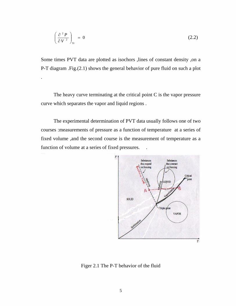
Some times PVT data are plotted as isochors ,lines of constant density ,on a

P-T diagram .Fig.(2.1) shows the general behavior of pure fluid on such a plot

.

The heavy curve terminating at the critical point C is the vapor pressure

curve which separates the vapor and liquid regions .

The experimental determination of PVT data usually follows one of two

courses :measurements of pressure as a function of temperature at a series of

fixed volume ,and the second course is the measurement of temperature as a

function of volume at a series of fixed pressures. .

Figer 2.1 The P-T behavior of the fluid

6

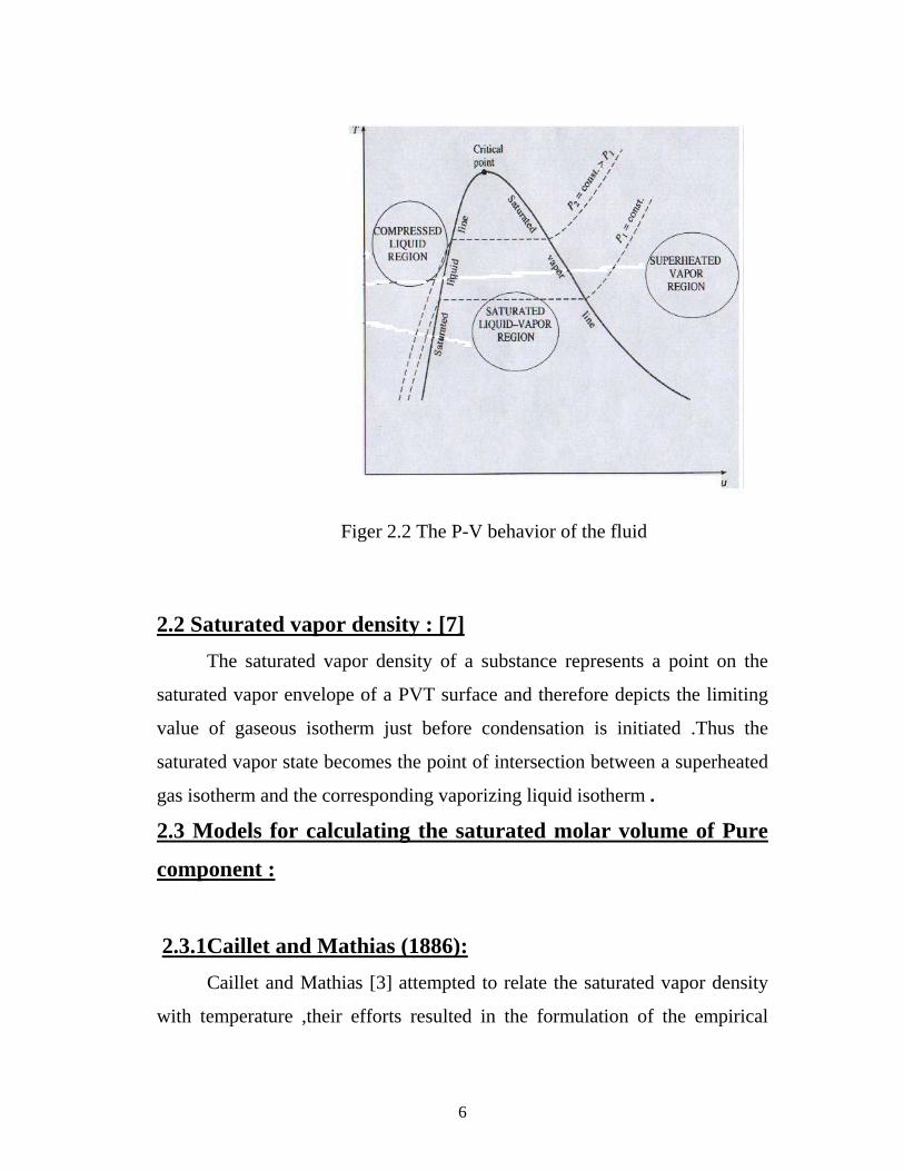
Figer 2.2 The P-V behavior of the fluid

2.2 Saturated vapor density : [7] The saturated vapor density of a substance represents a point on the

saturated vapor envelope of a PVT surface and therefore depicts the limiting

value of gaseous isotherm just before condensation is initiated .Thus the

saturated vapor state becomes the point of intersection between a superheated

gas isotherm and the corresponding vaporizing liquid isotherm .

2.3 Models for calculating the saturated molar volume of Pure

component :

2.3.1Caillet and Mathias (1886): Caillet and Mathias [3] attempted to relate the saturated vapor density

with temperature ,their efforts resulted in the formulation of the empirical

7

"rectilinear diameter rule " which states that the mean saturated density is

linearly dependent on temperature as follows :

KmTVL +=+ )(21 ρρ (2.3)

Where m and K are constants .

2.3.2 Bendict – Web – Rubin model :[42] ,[8]

Using Bendict-Web-Rubin equation of state to give analytical

expression for the volume . The vapor pressure data calculated from the

modified Antoine equation :

⎥⎥

⎦

⎤

⎢⎢

⎣

⎡⎟⎠⎞

⎜⎝⎛ ++

−+

−−+=

−2

23232

2

1*)/0(00 V

VVTC

VabRT

VTCARTB

VRTP

γ

γ (2.4)

Constants for the B-W-R equation have been determined by using least

squares method [47].

Comparison between the density from experimental data and the density

resulted from this equation ,for example for i-Pentane the deviation agrees

very well ,within 0.2% maximum difference .

2.3.3 Hirschfelder model (1958) : [46] The three expressions reported by Hirschofelder constitute a

generalized approach where each relationship is valid over

8

particular region of PVT surface . For 2601 selected values ,this equation of

state reproduces the densities with average deviation of 0.48% .These

deviations represent considerable improvement over corresponding values

obtained from the BWR equation of state and compare with those resulting

from the model proposed by Stewart (1981) .This model is qualitatively

correct and qualitatively exact and offers the most complete representation for

the PVT behavior of fluid.

The compressibility factor of this model is given by the following form

:

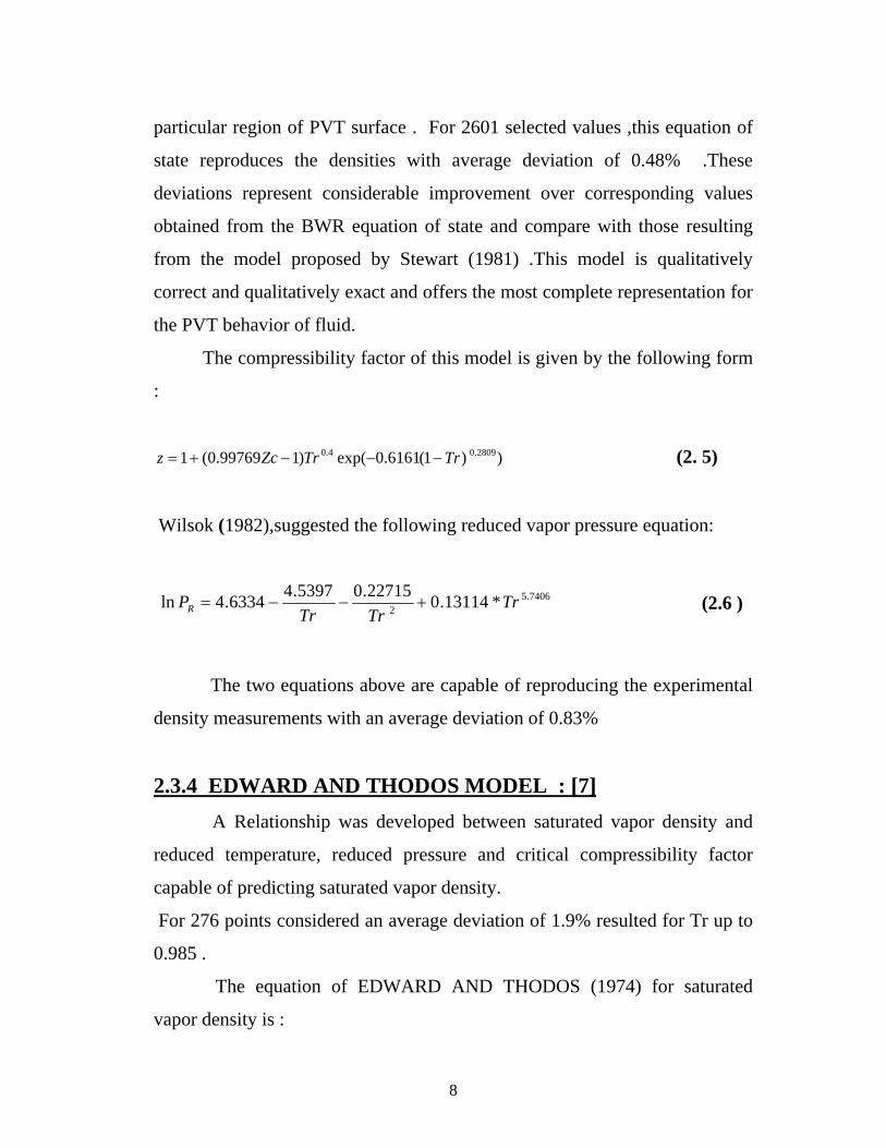
))1(6161.0exp()199769.0(1 2809.04.0 TrTrZcz −−−+= (2. 5)

Wilsok (1982),suggested the following reduced vapor pressure equation:

7406.52 *13114.022715.05397.46334.4ln Tr

TrTrPR +−−= (2.6 )

The two equations above are capable of reproducing the experimental

density measurements with an average deviation of 0.83%

2.3.4 EDWARD AND THODOS MODEL : [7] A Relationship was developed between saturated vapor density and

reduced temperature, reduced pressure and critical compressibility factor

capable of predicting saturated vapor density.

For 276 points considered an average deviation of 1.9% resulted for Tr up to

0.985 .

The equation of EDWARD AND THODOS (1974) for saturated

vapor density is :

9

⎥⎦

⎤⎢⎣

⎡−

−++= 33.63 )Pr2(

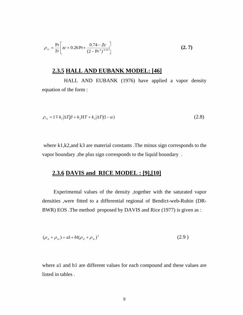
74.0Pr26.0Pr ZczcTrrvρ (2. 7)

2.3.5 HALL AND EUBANK MODEL: [46] HALL AND EUBANK (1976) have applied a vapor density

equation of the form :

)1(1 321 αβρ −∆+Η+∆= TkTkTkrs m (2.8)

where k1,k2,and k3 are material constants .The minus sign corresponds to the

vapor boundary ,the plus sign corresponds to the liquid boundary .

2.3.6 DAVIS and RICE MODEL : [9],[10]

Experimental values of the density ,together with the saturated vapor

densities ,were fitted to a differential regional of Bendict-web-Rubin (DR-

BWR) EOS .The method proposed by DAVIS and Rice (1977) is given as :

3)(11)( svslsvsl ba ρρρρ ++=+ (2.9 )

where a1 and b1 are different values for each compound and these values are

listed in tables .

10

This equation was tested with many experimental data of saturated

densities of many compounds such that for n-butane and n-pentane ,with

experimental data from saturated vapor and liquid density measurements of

Kay (1945)near the critical point and Liquid and vapor density measurements

of Sliwinski (1942)) and the results were acceptable with its error limits to 1%

.

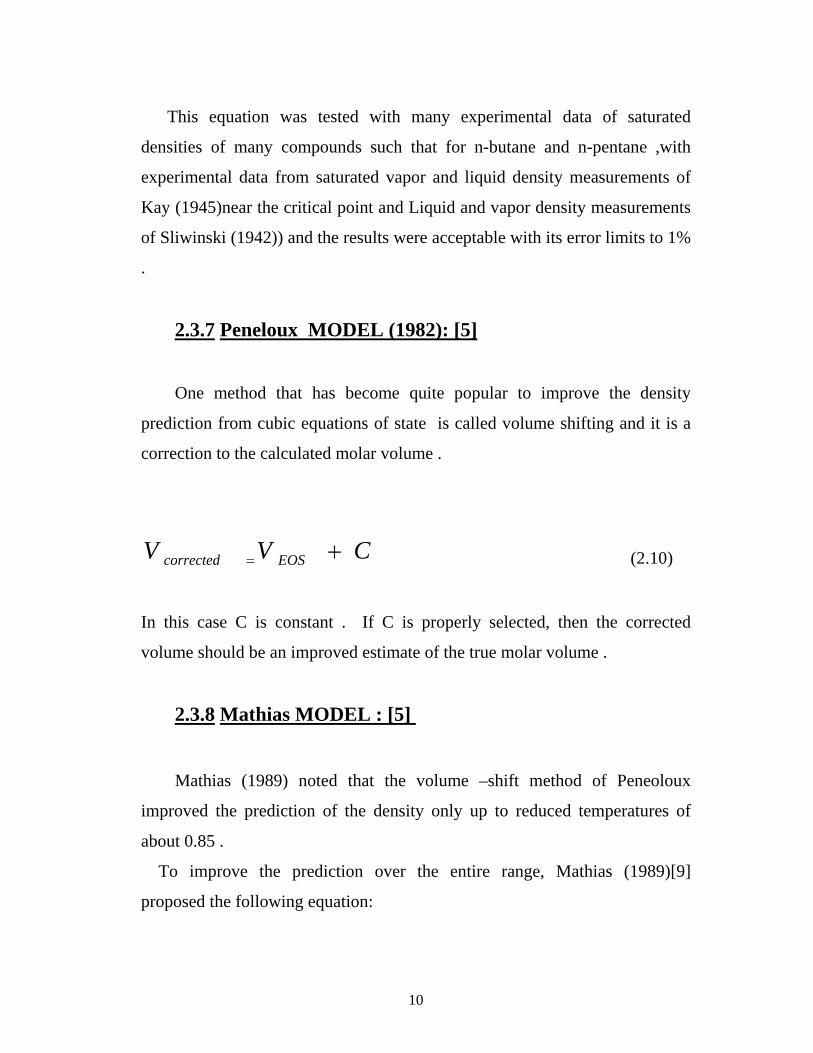
2.3.7 Peneloux MODEL (1982): [5]

One method that has become quite popular to improve the density

prediction from cubic equations of state is called volume shifting and it is a

correction to the calculated molar volume .

CVV EOScorrected += (2.10)

In this case C is constant . If C is properly selected, then the corrected

volume should be an improved estimate of the true molar volume .

2.3.8 Mathias MODEL : [5]

Mathias (1989) noted that the volume –shift method of Peneoloux

improved the prediction of the density only up to reduced temperatures of

about 0.85 .

To improve the prediction over the entire range, Mathias (1989)[9]

proposed the following equation:

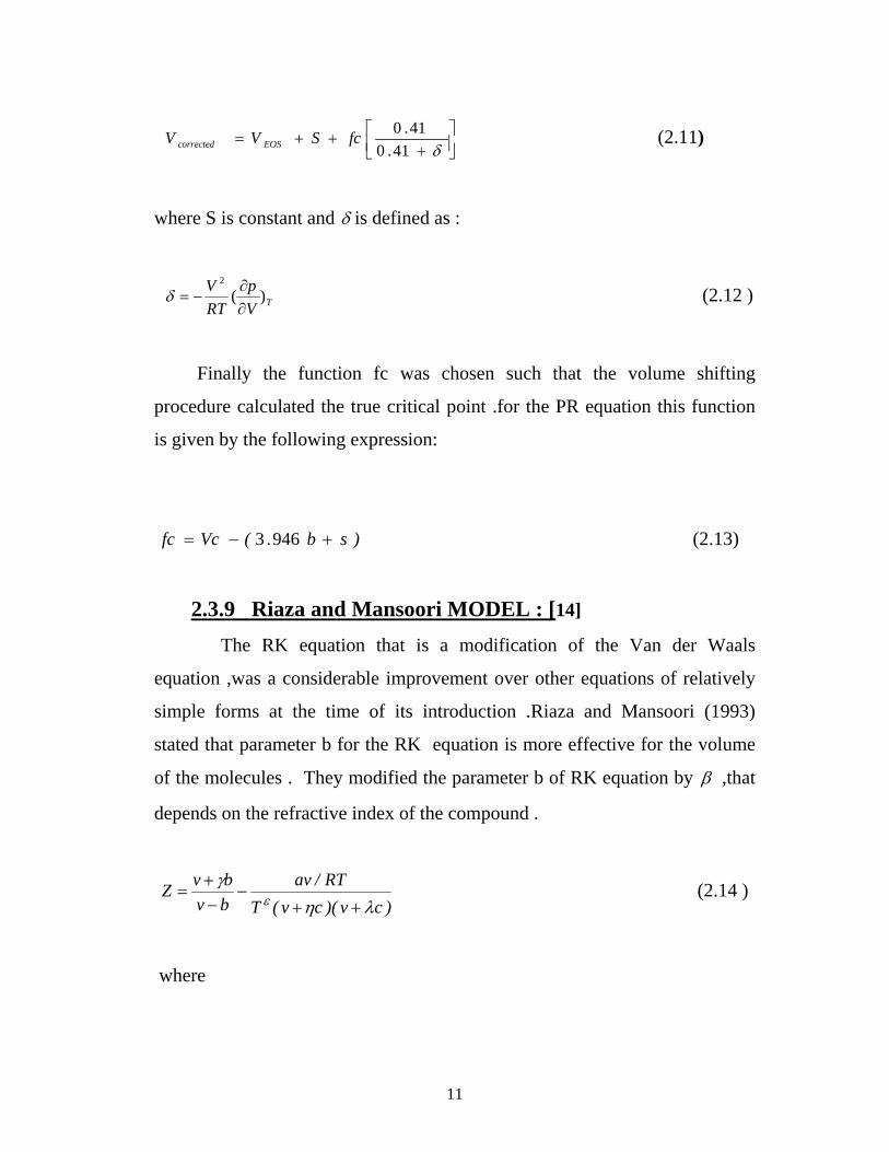
11

⎥⎦⎤

⎢⎣⎡

+++=

δ41.041.0fcSVV EOScorrected (2.11)

where S is constant and δ is defined as :

TVp

RTV )(

2

∂∂

−=δ (2.12 )

Finally the function fc was chosen such that the volume shifting

procedure calculated the true critical point .for the PR equation this function

is given by the following expression:

)sb.(Vcfc +−= 9463 (2.13)

2.3.9 Riaza and Mansoori MODEL : [14]

The RK equation that is a modification of the Van der Waals

equation ,was a considerable improvement over other equations of relatively

simple forms at the time of its introduction .Riaza and Mansoori (1993)

stated that parameter b for the RK equation is more effective for the volume

of the molecules . They modified the parameter b of RK equation by β ,that

depends on the refractive index of the compound .

)cv)(cv(T

RT/avbvbvZ

ληγ

ε ++−

−+

= (2.14 )

where

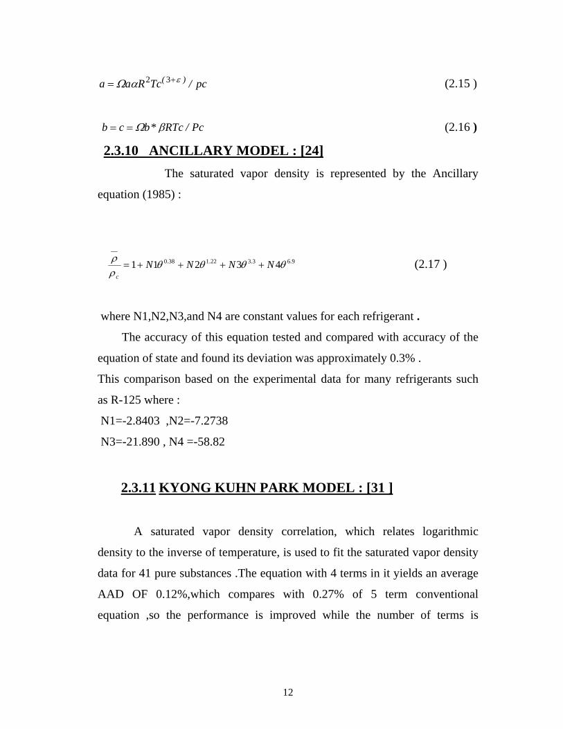
12

pc/TcRaa )( εαΩ += 32 (2.15 )

Pc/RTc*bcb βΩ== (2.16 )

2.3.10 ANCILLARY MODEL : [24] The saturated vapor density is represented by the Ancillary

equation (1985) :

9.63.322.138.0 43211 θθθθρρ NNNN

c

++++= (2.17 )

where N1,N2,N3,and N4 are constant values for each refrigerant .

The accuracy of this equation tested and compared with accuracy of the

equation of state and found its deviation was approximately 0.3% .

This comparison based on the experimental data for many refrigerants such

as R-125 where :

N1=-2.8403 ,N2=-7.2738

N3=-21.890 , N4 =-58.82

2.3.11 KYONG KUHN PARK MODEL : [31 ]

A saturated vapor density correlation, which relates logarithmic

density to the inverse of temperature, is used to fit the saturated vapor density

data for 41 pure substances .The equation with 4 terms in it yields an average

AAD OF 0.12%,which compares with 0.27% of 5 term conventional

equation ,so the performance is improved while the number of terms is

13

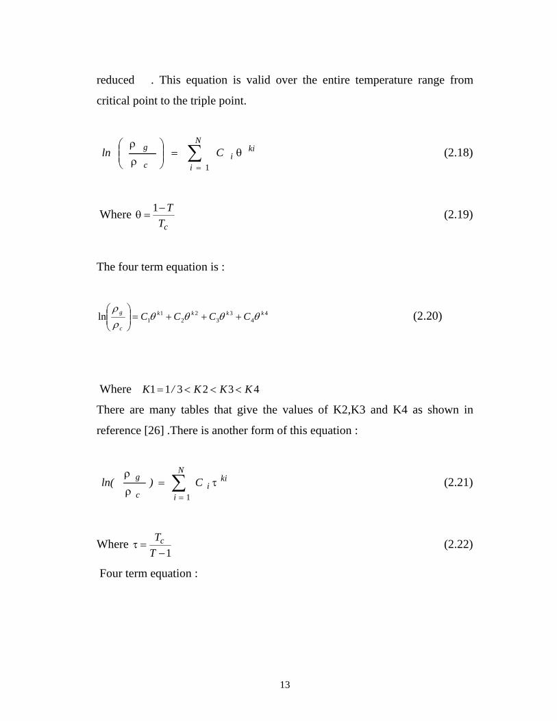
reduced . This equation is valid over the entire temperature range from

critical point to the triple point.

∑=

θ=⎟⎟⎠

⎞⎜⎜⎝

⎛ρ

ρ N

i

kii

c

g Cln1

(2.18)

Where cTT−

=θ1 (2.19)

The four term equation is :

44

33

22

11ln kkkk

c

g CCCC θθθθρρ

+++=⎟⎟⎠

⎞⎜⎜⎝

⎛ (2.20)

Where 432311 KKK/K <<<=

There are many tables that give the values of K2,K3 and K4 as shown in

reference [26] .There is another form of this equation :

∑=

τ=ρ

ρ N

i

kii

c

g C)ln(1

(2.21)

Where 1−

=τTTc (2.22)

Four term equation :

14

44

33

22

31ln kkkv

c

g CCCC ττττρρ

+++=⎟⎟⎠

⎞⎜⎜⎝

⎛ (2.23)

2.4 Molar volume for gas mixtures : [38] No comprehensive tests have been made of all estimation techniques.

Generally, errors were found to be less than 2 to 3 percent, except near the

critical point or for mixtures containing high polar components in significant

concentrations .Recommendations to estimate the molar volume of

hydrocarbon gas mixtures (including those component associated with natural

gas ,as CO2 and H2S ) , are essentially the same as for pure gases . for small

deviations from ideal-gas behavior , the truncated Virial equation is

satisfactory . Otherwise values of binary interaction coefficients (Kij's)

determined from VLE data can be used in volume calculations. Mixtures

molar volume is much less sensitive to Kij values than are VLE calculations .

There are many models that are developed to calculate the molar

volume of saturated vapors as follows :

2.4.1 Models for truncated Virial equation :

2.4.1.1 PITZ CURL model : [4] There are many mixing rules that can be used to calculate the molar

volume of binary mixtures . Pitz Curl calculated the density of binary

mixtures of hydrocarbon gases according to a aforementioned method by

using Virial equation truncated to third term .

21 expmixexpmix *C*B(RT

Pcalρ+ρ+

=ρ

(2.24)

15

2.4.1.2GERG method [4]: This equation is based on three-term truncated Virial equation,

it predicts the density of mixtures up to 13 common components of natural

gas with an estimated uncertainty of 0.1% :

21 exp*mixexpmix C*BZ ρ+ρ+= (2.25)

ZRT

Pcal =ρ (2.26)

\

2.4.2 Methods based on volume –shifting method :

2.4.2.1 Peneloux model for mixture :[ 5] To apply this method to the mixtures, it is assumed that C for the

mixture, C mix is the mole fraction weighted as average of the parameters for

the pure components.

∑=

=Nc

iiimix CxC

1* (2.27)

Then substituting this in the Peneoloux equation:

mixEOSsformixture

corrected CVV += (2.28)

16

2.4.2.2 Mathias model for mixture: [5] To apply this method to mixtures, it is assumed that:

∑=

=Nc

iiimix SXS

1* (2.29)

Then substituting this value in the Mathias equation :

⎥⎦⎤

⎢⎣⎡

δ+++=

410410

..fSVV cmixEOS

formixturecorrected (2.30)

17

CHAPTER THREE

Theories and Definitions

3.1 Equation of state :[ 46],[38] The term equation of state means an equation that relates volume to

pressure and temperature .

The simplest equation of state is ideal gas equation :

PV=nRT (3.1)

This equation is only true at zero pressure .

Many equation of state of varying degrees of complexity have been

proposed and while a few have some basis in molecular theory ,all are used

empirically .the advantages offered by equation of state are mainly data

reduction and ease of use in subsequent calculations .

A large number of PVT equations have been developed to describe

non-ideal or real gas behavior.

3.2 Classification of Equations of state : [4] The need for accurate prediction of the thermodynamic properties of

many fluids and mixtures has led to the development of equations of state

with different forms .before proceeding with the discussion of specific

equations of state it is useful to make some general classification in to which

they may fall.

18

The main types of equation of state may be classified conveniently

according to their mathematical form as follows:

3.2.1 :Standerd P-V-T forms :

This type of equation of state may be written for a pure fluid as :

P=p(T, mV ) or Z=Z(T, mV ) ( 3.2)

a. Truncated Virial equation in which p is given by polynomial in mV/1 with

temperature and composition dependent coefficients.

b. Complex empirical equations: which represent p by some combination of

polynomial and other term (e.g. BWR and related equations).

It is also possible to invert the functional relationships to give mV or Z in

terms of T,P and the composition variables .However ,although this choice

of independent variables may be convenient in the analysis of

experimental data for a single fluid phase ,it is almost never used in

thermodynamic modeling .

3.2.2 Fundamental form : A fundamental equation gives one of the state functions in terms of its

natural independent variables .The most common choice is the molar

Helmoltz energy Am as a function of temperature and the molar volume .

mA = mA (T, mV ) (3.3)

In order to achieve a precise representation of the experimental data

over a wide range of conditions ,the structure of the functional relationship is

19

often very complicated ,Am is split into perfect gas and residual parts which

are parameterized separately .

Although accurate fundamental equations of state exist for only about

twenty of the most important pure fluids ,one or more of these may form the

basis of a corresponding states treatment of the residual properties of a wide

variety of other fluids including mixtures .

3.3 Law of corresponding states :[38] The principle of corresponding states establishes a connection between

the configuration integrals of different substances and thereby allows each of

configurationally and residual thermodynamic properties are related in a very

simple way .

The assumption in applying corresponding states is that the PVT

behavior of the mixture will be the same as that of pure component whose

critical temperature and pressure are equal to the pseudo critical temperature

and pressure of the mixture .

To apply the corresponding states to the mixture ,one must determine

appropriate scaling factor.

3.3.1 Two parameter correlations (spherical molecules): [

38],[4] The non ideality of the gas is conveniently expressed by the

compressibility factor z .

20

The compressibility factor is often correlated with Tr,Pr as :

Z=f(Tr,Pr) (3.4)

equation (3.6) is an example of the law of corresponding states in this

equation Vr is not defined in the usual manner ,that is ,(V/Vc),but instead is

an "ideal reduced volume "given by :

(3.5)

This law ,though not exact ,suggest that reduced properties of all fluids

are essentially the same if compared at equal reduced temperature and

pressures :

for PVT properties ,this law gives :

Cr V

VV = =C

CC

ppTTZZ

/)/)(/(

= 1f (Tr,Pr) (3.6)

Z=Zc 2f (Tr,Pr) (3.7)

Except for monatomic gases ,highly polar fluids ,and fluids composed of large

molecules ,value of zc for most organic compounds range form .27 to .29 if it

is assumed to be a constant .

pcRTcVVri

/=

21

3.3.2 Three parameter correlations (non spherical molecules):[

51],[39]

In general successful Eos have included one or more dimensionless

characteristic parameters in to the function the first step in accomplishing this

is to introduce a third parameter ; usually it is related to the vapor pressure

,Pvp ,or volumetric property at or near the critical point .

Historically several different third parameters were introduced at about the

same time but the most popular have been zc (lyderson,1955) and the

acentric factor w(Pitzer and Curl 1955,1057 ab).Lyderson and later revision

by Hougan ,et .al.(1959) tabulated z (and reduced thermodynamic properties )

at increment of (Tr) and (Pr)for different values of zc in practice, this

correlation has been used only occasionally ,such as by Edward and Thodos

(1974)for estimating saturated vapor densities of non polar compounds .

The much more commonly used third parameter is the acentric factor .

for example the compressibility factor was given as :

(3.8)

3.3.3 Four parameter model (polar molecules) :[ 4] WU and Stiel[52]modified the Lee-kesler[24]scheme by incorporating

the polar substance water as a third reference fluid .The compression factor is

given by :

( 3.9)

Pr),(1Pr),(0 TrzTrzz ω+=

210 zzzz γω ++=

22

Where γ is a fourth parameter characteristic of polar molecules . Here ,z0 and

z1 are given by the original Lee-kesler scheme ,while z2 was defined in terms

of the compression factor Zw of water by means of the equation :

(3.10)

In which ω =0.344 is the acentric factor of the water .

This definition ensures that for non-polar systems ,the compression

factor reverts to the Lee-Kesler formulation while ,for )1( =γ ,eq .(3.9)

reduced to the compression factor zw of water .

WU and Stile argued that a definition based on the molar volume of the

saturated liquid at specified reduced temperature had the desired properties

.thus they defined γ by means of equation :

γσ 0222.0547.1326. −−=vr (3.11)

Where )(C

Cmr RT

PVV δδ = (3.12)

3.4 Van der waals Equation : [22] Undoubtedly ,the best known equation of state is the Van der Waals

equation :

(3.13)

)10(2 wzzzz ωω +−=

2Va

bVRTp −−

=

23

according to Van der Waals derivation .The term (a/v2)accounts for attractive

forces between molecules ,and b is a correction for the volume occupied by

the molecules themselves .This equation is cubic in v ,and at temperatures

below the critical there are three real root ,as indicated in fig (2.1) it can be

shown that the segment of the isotherm lying between A and B represents

unstable state ,and therefore in the pressure range PA to PB there are only two

values of v which correspond to stable states.

While this suggests the application of Van der waals equation to

calculations in the two phase region ,the form of the equation is far too simple

to be capable of closely representing the isotherm in this region.

When an equation of state contain only two parameters in the term of

critical temperature and pressure. Evaluating these derivatives and the

equation of state at the critical point results in three equations involving

a,b,tc,pc and Vc .Because Vc is not always available .It can be eliminated at

the remaining equations solved for a ,and b in terms of Tc and Pc .for Van

der waals equation this results in :

C

C

PTR

a64

27 22

=

, Pc

RTcb8

= (3.14)

Because Tc and Pc are known as for many substances ,it is convenient to

evaluate parameters in this manner .

24

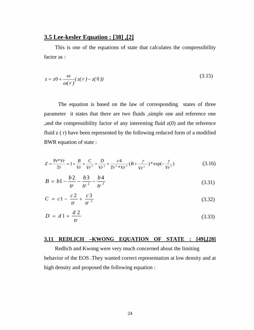
3.5 Lee-kesler Equation : [38] ,[2] This is one of the equations of state that calculates the compressibility

factor as :

(3.15)

The equation is based on the law of corresponding states of three

parameter it states that there are two fluids ,simple one and reference one

,and the compressibility factor of any interesting fluid z(0) and the reference

fluid z ( r) have been represented by the following reduced form of a modified

BWR equation of state :

)exp(*)(*41Pr*

222332 VrVrB

VrTrc

VrD

VrC

VrB

TrVrZ γγ

−+++++== (3.16)

324321

trb

trb

trbbB −−−= (3.31)

3321

trc

trccC +−= (3.32)

trddD 21 += (3.33)

3.11 REDLICH –KWONG EQUATION OF STATE : [49],[28]

Redlich and Kwong were very much concerned about the limiting

behavior of the EOS .They wanted correct representation at low density and at

high density and proposed the following equation :

))(z)r(z()r(

zz 00 −+=ωω

25

,/,/)( 5.225.0 PcTcaRacTaT C Ω==α (3.34)

0867.,4278. =Ω=Ω ba (3.35)

PcbRTcb /Ω= (3.36)

This equation did not have strong theoretical background but proved

to give good results for many gaseous systems ,it should be also mentioned

that ,when Redlich and Kwong proposed their celebrated equation of state

they were inserted in developing a good equation for gases only .

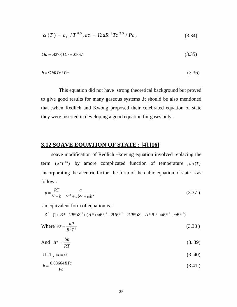
3.12 SOAVE EQUATION OF STATE : [4],[16] soave modification of Redlich –kowing equation involved replacing the

term )/( 5.0Ta by amore complicated function of temperature , )(Taα

,incorporating the acentric factor ,the form of the cubic equation of state is as

follow :

22 bubVVa

bVRTp

ω++−

−= (3.37 )

an equivalent form of equation is :

)*****)2*2**(*)*1( 322223 BBBAZUBUBBAZUBBZ ωωω −−−−−++−+−

Where 22*TR

aPA = (3.38 )

And RTbp*B = (3. 39)

U=1 , 0=ω (3. 40)

Pc

RTcb 08664.0= (3.41 )

26

and [ ]25.022

)1(1**42748.0 TrfwPc

TcRa −+= (3.42)

2176.0574.148.0 ωω −+=fw (3.43 )

The form of this function was devised primarily to obtain a good

representation of the vapor pressure curve for a number of hydrocarbons

.Subsequently ,this term was modified further by Graboski and Daubert

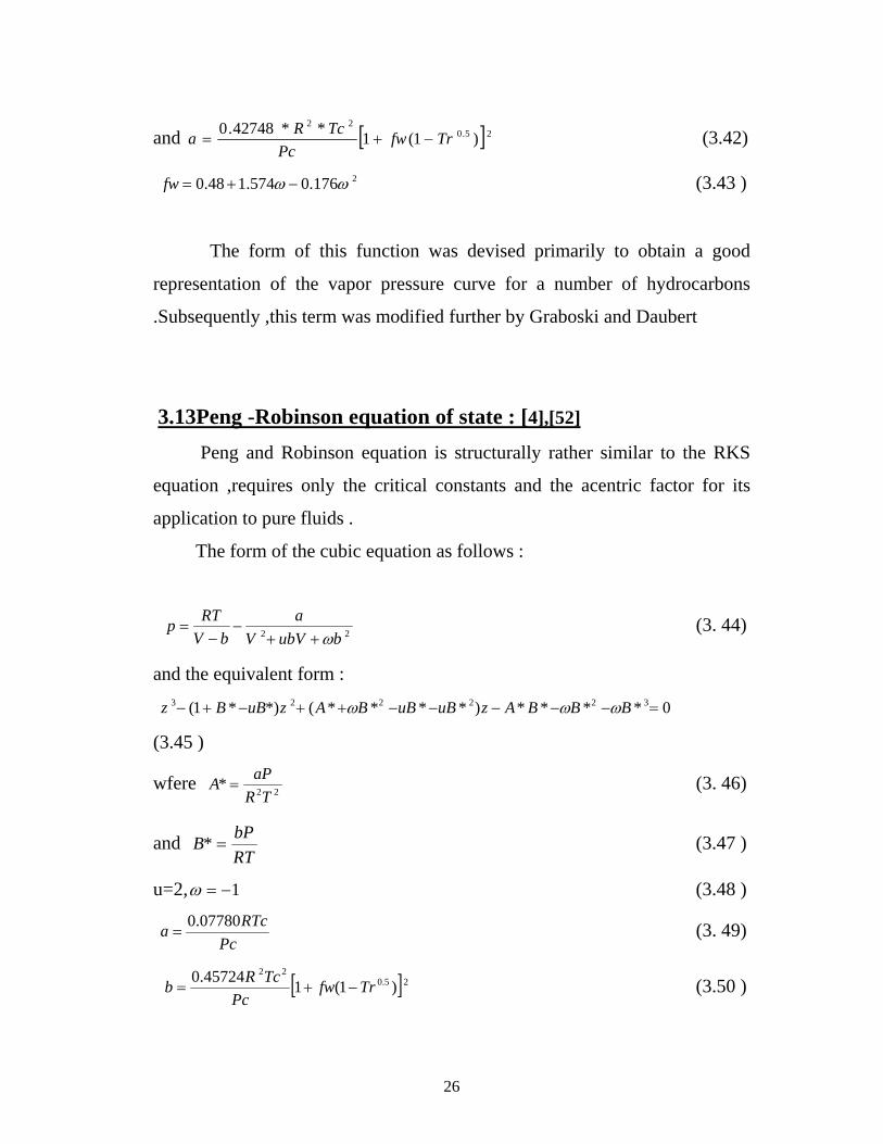
3.13Peng -Robinson equation of state : [4],[52]

Peng and Robinson equation is structurally rather similar to the RKS

equation ,requires only the critical constants and the acentric factor for its

application to pure fluids .

The form of the cubic equation as follows :

22 bubVVa

bVRTp

ω++−

−= (3. 44)

and the equivalent form :

0****)****(*)*1( 322223 =−−−−−++−+− BBBAzuBuBBAzuBBz ωωω

(3.45 )

wfere 22*TR

aPA = (3. 46)

and RTbP*B = (3.47 )

u=2, 1−=ω (3.48 )

Pc

RTca 07780.0= (3. 49)

[ ]25.022

)1(145724.0 TrfwPc

TcRb −+= (3.50 )

27

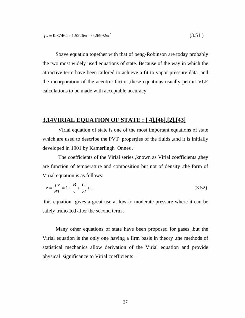
226992.05226.137464.0 ωω −+=fw (3.51 )

Soave equation together with that of peng-Robinson are today probably

the two most widely used equations of state. Because of the way in which the

attractive term have been tailored to achieve a fit to vapor pressure data ,and

the incorporation of the acentric factor ,these equations usually permit VLE

calculations to be made with acceptable accuracy.

3.14VIRIAL EQUATION OF STATE : [ 4],[46],[2],[43] Virial equation of state is one of the most important equations of state

which are used to describe the PVT properties of the fluids ,and it is initially

developed in 1901 by Kamerlingh Onnes .

The coefficients of the Virial series ,known as Virial coefficients ,they

are function of temperature and composition but not of density .the form of

Virial equation is as follows:

....vC

vB

RTpvz +++==

21 (3.52)

this equation gives a great use at low to moderate pressure where it can be

safely truncated after the second term .

Many other equations of state have been proposed for gases ,but the

Virial equation is the only one having a firm basis in theory .the methods of

statistical mechanics allow derivation of the Virial equation and provide

physical significance to Virial coefficients .

28

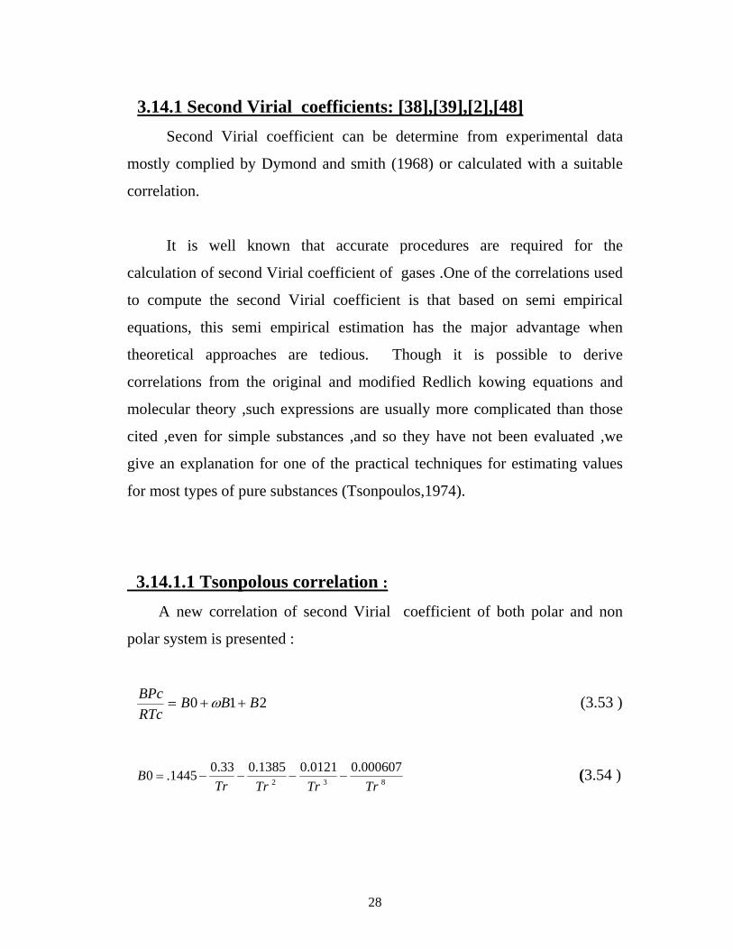
3.14.1 Second Virial coefficients: [38],[39],[2],[48] Second Virial coefficient can be determine from experimental data

mostly complied by Dymond and smith (1968) or calculated with a suitable

correlation.

It is well known that accurate procedures are required for the

calculation of second Virial coefficient of gases .One of the correlations used

to compute the second Virial coefficient is that based on semi empirical

equations, this semi empirical estimation has the major advantage when

theoretical approaches are tedious. Though it is possible to derive

correlations from the original and modified Redlich kowing equations and

molecular theory ,such expressions are usually more complicated than those

cited ,even for simple substances ,and so they have not been evaluated ,we

give an explanation for one of the practical techniques for estimating values

for most types of pure substances (Tsonpoulos,1974).

3.14.1.1 Tsonpolous correlation : A new correlation of second Virial coefficient of both polar and non

polar system is presented :

210 BBBRTcBPc

++= ω (3.53 )

832

000607.00121.01385.033.01445.0TrTrTrTr

B −−−−= (3.54 )

29

832

008.0423.0331.00637.01TrTrTr

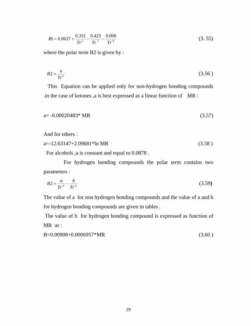
B −−+= (3. 55)

where the polar term B2 is given by :

62TraB = (3.56 )

This Equation can be applied only for non-hydrogen bonding compounds

.in the case of ketones ,a is best expressed as a linear function of MR :

a= -0.00020483* MR (3.57)

And for ethers :

a=-12.63147+2.09681*ln MR (3.58 )

For alcohols ,a is constant and equal to 0.0878 .

For hydrogen bonding compounds the polar term contains two

parameters :

862Tr

bTr

aB −= (3.59)

The value of a for non hydrogen bonding compounds and the value of a and b

for hydrogen bonding compounds are given in tables .

The value of b for hydrogen bonding compound is expressed as function of

MR as :

B=0.00908+0.0006957*MR (3.60 )

30

CROSS COEFFICIENTS FOR MIXTURES :

The second Virial cross coefficient Bij has the same temperature

dependence that Bii and Bjj have ,but the parameters to be used are

Tcij, ijω ,aij and bij .

The mixing rule are given below :

Tcj.Tci)Kij(Tcij −= 1 (3. 61)

33/1 )3/1(

**4

VcjVciTcj

VcjPcjTci

VciPciTcijPcij

+

⎥⎦

⎤⎢⎣

⎡+

= (3.62 )

)(5.0 jiij ωωω += (3.63 )

For polar/non polar binary mixture ,Bij is assumed to have no polar

term :aij=0 (3.64 )

bij=0 (3.65 )

For polar/polar binary mixtures, the polar contribution to bij is

calculated by assuming that :

aij= 0.5(ai+aj) (3.66 )

bij=0.5(bi+bj) (3.67 )

3.14.2 Third virial coefficient: [39],[30],[17] It is possible to derive the third Virial coefficient correlations from

molecular theory ,but these are not very successful .

The principle theoretical problem is that the trio intermolecular potential

includes significant contributions that can not be determined from their pair

potentials that describe second Virial coefficients .Thus ,CSP is also used

31

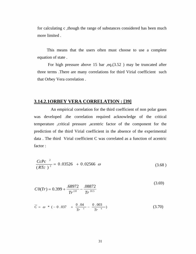
for calculating c ,though the range of substances considered has been much

more limited .

This means that the users often must choose to use a complete

equation of state .

For high pressure above 15 bar ,eq.(3.52 ) may be truncated after

three terms .There are many correlations for third Virial coefficient such

that Orbey Vera correlation .

3.14.2.1ORBEY VERA CORRELATION : [39] An empirical correlation for the third coefficient of non polar gases

was developed .the correlation required acknowledge of the critical

temperature ,critical pressure ,acentric factor of the component for the

prediction of the third Virial coefficient in the absence of the experimental

data . The third Virial coefficient C was correlated as a function of acentric

factor :

ω02566.003526.0)( 2

2

+=RTc

CcPc (3.68 )

(3.69)

C )003.004.0037.0(* 63 TrTr−+−= ω (3.70)

5.108.208872.68972.399.0)(0TrTr

TrC −+=

32

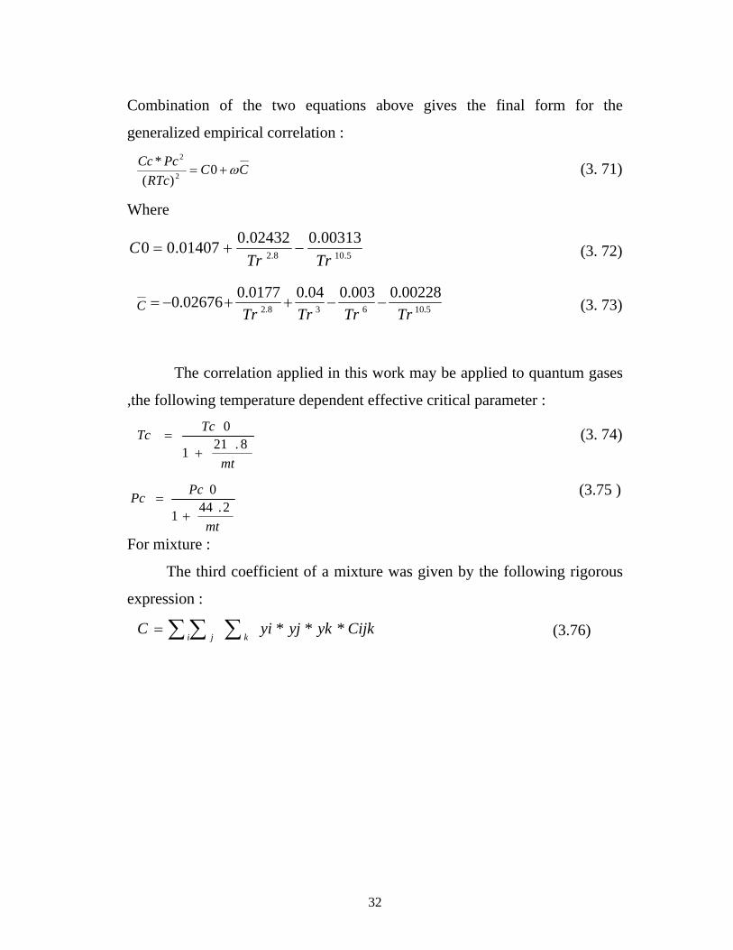
Combination of the two equations above gives the final form for the

generalized empirical correlation :

CCRTc

PcCc ω+= 0)(

*2

2

(3. 71)

Where

5.108.2

00313.002432.001407.00TrTr

C −+= (3. 72)

C 5.10638.200228.0003.004.00177.002676.0

TrTrTrTr−−++−= (3. 73)

The correlation applied in this work may be applied to quantum gases

,the following temperature dependent effective critical parameter :

mt

TcTc8.211

0

+= (3. 74)

(3.75 )

For mixture :

The third coefficient of a mixture was given by the following rigorous

expression :

CijkykyjyiCi kj

***∑ ∑∑= (3.76)

mt

PcPc2.441

0

+=

33

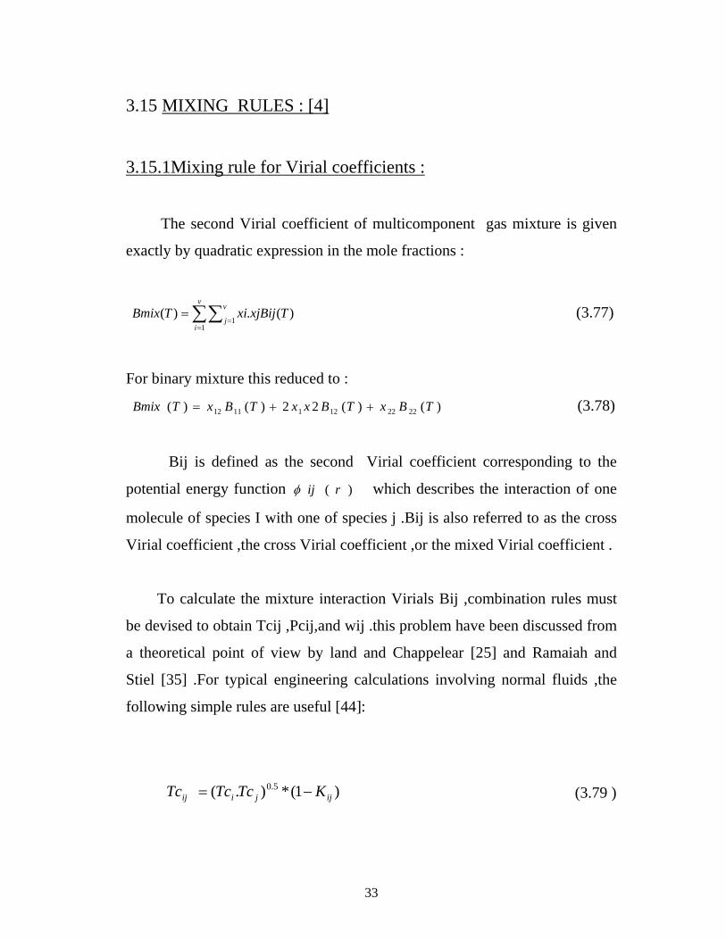
3.15 MIXING RULES : [4]

3.15.1Mixing rule for Virial coefficients :

The second Virial coefficient of multicomponent gas mixture is given

exactly by quadratic expression in the mole fractions :

∑∑=

==

v

i

v

jTxjBijxiTBmix

11

)(.)( (3.77)

For binary mixture this reduced to :

)()(22)()( 22221211112 TBxTBxxTBxTBmix ++= (3.78)

Bij is defined as the second Virial coefficient corresponding to the

potential energy function )( rijφ which describes the interaction of one

molecule of species I with one of species j .Bij is also referred to as the cross

Virial coefficient ,the cross Virial coefficient ,or the mixed Virial coefficient .

To calculate the mixture interaction Virials Bij ,combination rules must

be devised to obtain Tcij ,Pcij,and wij .this problem have been discussed from

a theoretical point of view by land and Chappelear [25] and Ramaiah and

Stiel [35] .For typical engineering calculations involving normal fluids ,the

following simple rules are useful [44]:

)1(*).( 5.0ijjiij KTcTcTc −= (3.79 )

34

23/13/1

2.

⎥⎦

⎤⎢⎣

⎡=

VcjVciVcij (3.80)

2ZcjZciZcij +

= (3.81 )

2jiij ωωω +

= (3.82)

VcijZcijRTcijPcij = (3. 83)

33/13/1

5.0

)().(81

VcjVciVcjVciKij+

−= (3. 84)

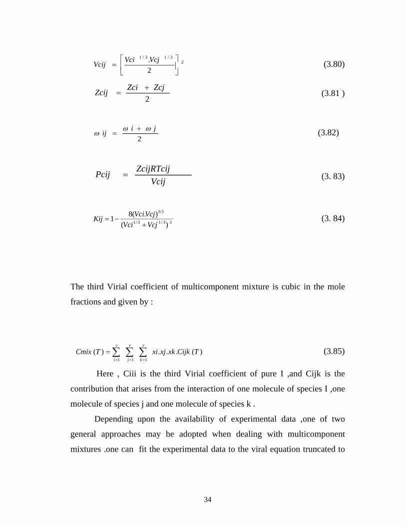
The third Virial coefficient of multicomponent mixture is cubic in the mole

fractions and given by :

)(...)(111

TCijkxkxjxiTCmixv

k

v

j

v

i∑∑∑===

= (3.85)

Here , Ciii is the third Virial coefficient of pure I ,and Cijk is the

contribution that arises from the interaction of one molecule of species I ,one

molecule of species j and one molecule of species k .

Depending upon the availability of experimental data ,one of two

general approaches may be adopted when dealing with multicomponent

mixtures .one can fit the experimental data to the viral equation truncated to

35

the third coefficient and obtain each of the possible pure component and

interaction Virial coefficients .

This requires experimental data for each of the possible binary and

ternary combinations of the components .

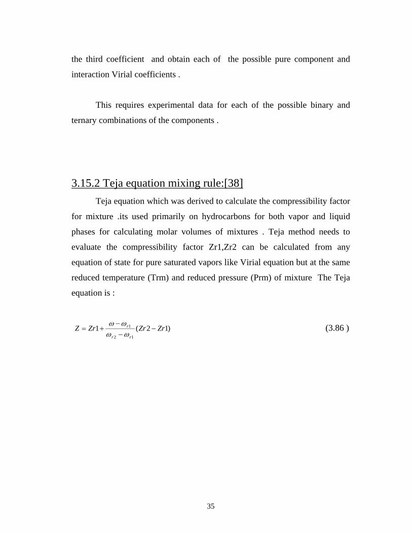
3.15.2 Teja equation mixing rule:[38] Teja equation which was derived to calculate the compressibility factor

for mixture .its used primarily on hydrocarbons for both vapor and liquid

phases for calculating molar volumes of mixtures . Teja method needs to

evaluate the compressibility factor Zr1,Zr2 can be calculated from any

equation of state for pure saturated vapors like Virial equation but at the same

reduced temperature (Trm) and reduced pressure (Prm) of mixture The Teja

equation is :

)12(112

1 ZrZrZrZrr

r −−−

+=ωωωω (3.86 )

36

CHAPTER FOUR

Investigation and Development

4.1 investigation of the equations of state : Vapor densities can be calculated from equations of state.

Usually the accuracy of some equations of state to calculate the

saturated molar volumes of pure components is not satisfactory . on

the other hand the accuracy of many models of equations of state are

not good enough for mixtures, mainly due to the problems in

formulating the mixing rule .

It is well known fact that the evaluation of any correlation or

prediction method is done by comparison of the results obtained from

the correlation with those results obtained from the experimental data

which will measure the accuracy of this prediction .The experimental

data needed in this prediction is PVT data for pure components and

PVTX for mixtures at saturation conditions .

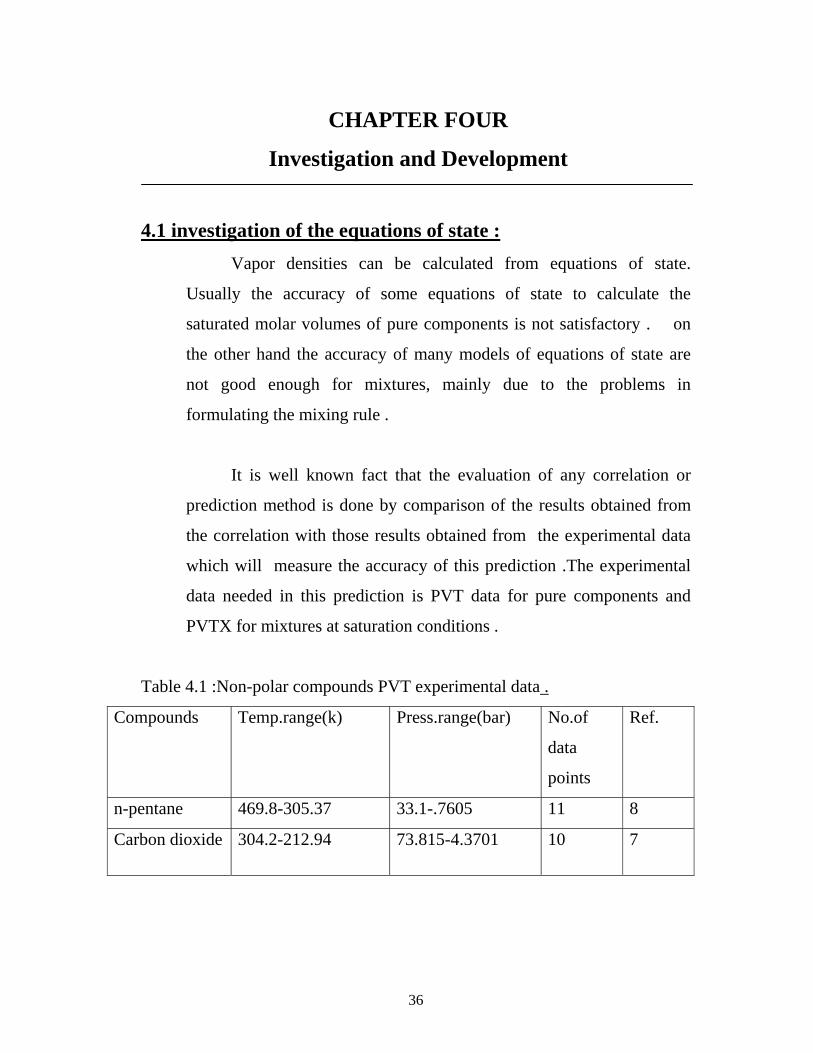
Table 4.1 :Non-polar compounds PVT experimental data .

Compounds Temp.range(k) Press.range(bar) No.of

data

points

Ref.

n-pentane 469.8-305.37 33.1-.7605 11 8

Carbon dioxide 304.2-212.94 73.815-4.3701 10 7

37

Carbon

monoxide

131.705-73.26 31.202-.3415 12 7

Ref.410 173.15-204.15 0.037-0.382 32 19

n-butane 272.67-420 1.01325-34.946 25 8

Neopentane 282.628-431 1.01325-30.632 23 36

Cyclo propane 357.03-380.46 44.4155-71.058 28 26

i-pentane 255.372-365.92 0.1502-601980 21 7

Ref.245 232.59-333.705 0.3493-3.005 16 42

i-butane 261.32-400 1.01325-301927 21 8

Table 4.2 :Polar compounds PVT experimental data .

Compound Temp.range(k) Press.range(bar) No.of

data

points

Ref.

Water 263.15-305.37 0.00286-1.0505 23 6

Propanol 304.2-212.94 0.02683-41.255 24 29

Propyl

alcohol

277.59-377.59 0.08-19.078 20 25

ammonia 357.03-394.91 45-94 33 13

There are several equations of state that are used to describe the

thermodynamic properties of the fluids ,such as Lee-Kesler ,Soave ,Peng

Robinson ,Truncated Virial equation, and many other equations of state

38

.These equations are considered the most important and accurate equations

that are used to determined the thermodynamic properties of the fluids (liquid

and vapor phases ) .

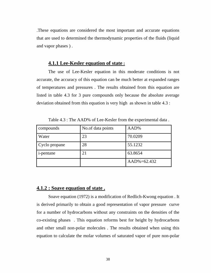
4.1.1 Lee-Kesler equation of state :

The use of Lee-Kesler equation in this moderate conditions is not

accurate, the accuracy of this equation can be much better at expanded ranges

of temperatures and pressures . The results obtained from this equation are

listed in table 4.3 for 3 pure compounds only because the absolute average

deviation obtained from this equation is very high as shown in table 4.3 :

Table 4.3 : The AAD% of Lee-Kesler from the experimental data .

compounds No.of data points AAD%

Water 23 70.0209

Cyclo propane 28 55.1232

i-pentane 21 63.8654

AAD%=62.432

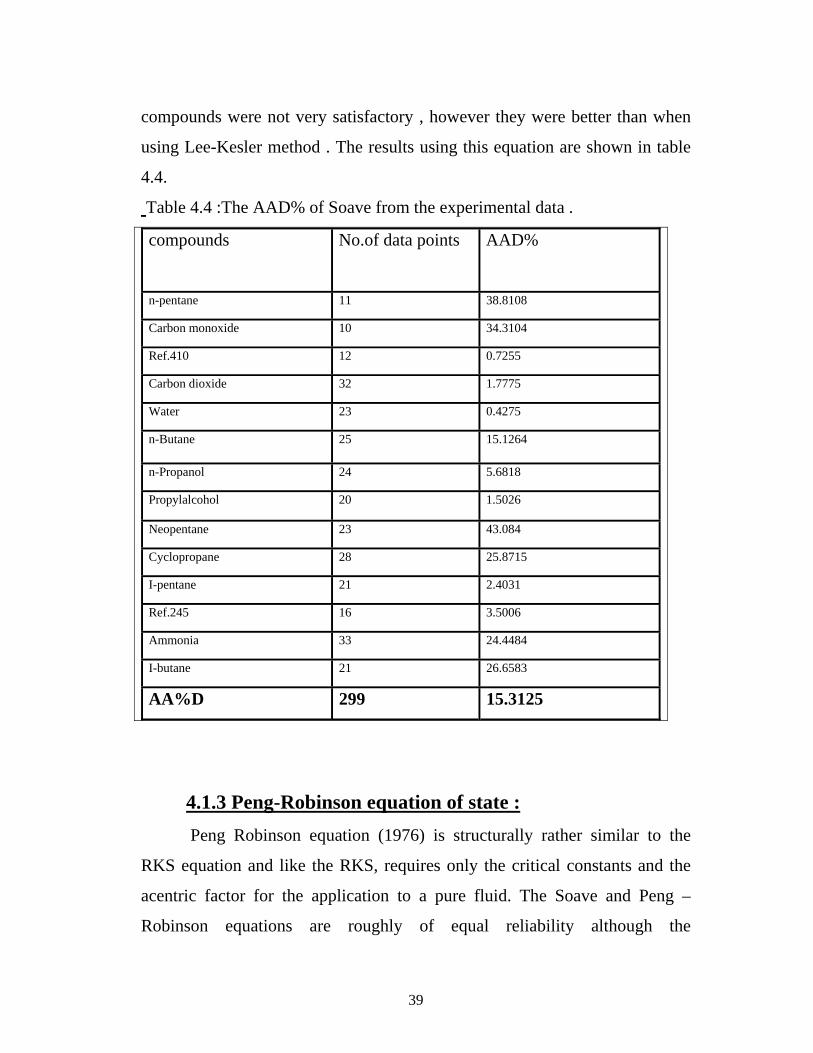
4.1.2 : Soave equation of state . Soave equation (1972) is a modification of Redlich-Kwong equation . It

is derived primarily to obtain a good representation of vapor pressure curve

for a number of hydrocarbons without any constraints on the densities of the

co-existing phases . This equation reforms best for height by hydrocarbons

and other small non-polar molecules . The results obtained when using this

equation to calculate the molar volumes of saturated vapor of pure non-polar

39

compounds were not very satisfactory , however they were better than when

using Lee-Kesler method . The results using this equation are shown in table

4.4.

Table 4.4 :The AAD% of Soave from the experimental data .

compounds No.of data points AAD%

n-pentane 11 38.8108

Carbon monoxide 10 34.3104

Ref.410 12 0.7255

Carbon dioxide 32 1.7775

Water 23 0.4275

n-Butane 25 15.1264

n-Propanol 24 5.6818

Propylalcohol 20 1.5026

Neopentane 23 43.084

Cyclopropane 28 25.8715

I-pentane 21 2.4031

Ref.245 16 3.5006

Ammonia 33 24.4484

I-butane 21 26.6583

AA%D 299 15.3125

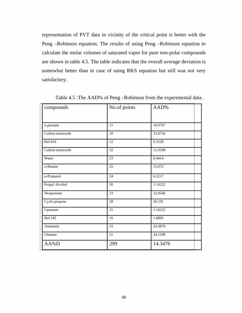
4.1.3 Peng-Robinson equation of state : Peng Robinson equation (1976) is structurally rather similar to the

RKS equation and like the RKS, requires only the critical constants and the

acentric factor for the application to a pure fluid. The Soave and Peng –

Robinson equations are roughly of equal reliability although the

40

representation of PVT data in vicinity of the critical point is better with the

Peng –Robinson equation. The results of using Peng –Robinson equation to

calculate the molar volumes of saturated vapor for pure non-polar compounds

are shown in table 4.5. The table indicates that the overall average deviation is

somewhat better than in case of using RKS equation but still was not very

satisfactory.

Table 4.5 :The AAD% of Peng –Robinson from the experimental data .

compounds No.of points AAD%

n-pentane 11 18.0767

Carbon monoxide 10 33.0754

Ref.410 12 0.5528

Carbon monoxide 32 11.0508

Water 23 0.4414

n-Butane 25 15.072

n-Propanol 24 6.5217

Propyl Alcohol 20 1.14222

Neopentane 23 32.0546

Cyclo propane 28 26.191

I-pentane 21 1.14222

Ref.245 16 1.6895

Ammonia 33 24.3876

I-butane 21 24.1598

AA%D 299 14.3476

41

4.1.4 Truncated Virial equation of state : Truncated Viral equation is one of the most important equations of state

that are used to describe the PVT properties of the vapor phase .It is found

that truncated Virial equation is the best equation to calculate the molar

volumes of the saturated vapor, Virial equation truncated to the second

coefficient,and Virial equation truncated to the third coefficient gives very

accurate results that reduced the average deviation from the previous

equations of state as considered in table 4.6 .

Table 4.6 : The AAD% of Virial truncated to second and third

coefficient from the experimental data .

compounds No.of

Data points

AA%D

truncated at B

AA%D

truncated at C

n-pentane 11 9.9576 0.9088

Carbon monoxide 10 6.190603 1.5539

Carbon dioxide 12 25.7386 0.5922

Ref.410 32 0.42185 0.6737

Water 23 0.5425 0.1884

n-Butane 25 15.072 1.1236

n-Propanol 24 6.5217 1.4087

Propylalcohol 20 1.1945 0.8735

Neopentane 23 32.0546 1.7228

Cyclopropane 28 9.2764 1.8200

I-pentane 21 0.3274 1.6740

Ref.245 16 0.9546 0.50607

Ammonia 33 3.4504 0.9296

I-butane 21 2.9531 1.19848

AA%D 299 7.5525 1.0955

42

The comparison in appendix C indicates that Soave and Peng –

Robinson accuracy increase when temperature and pressure range decreases

and the equation losses the accuracy when calculating for higher temperatures

and pressures . This finding is shown clearly when observing that the Virial

equation results are closer to the experimental PVT data. It was found that the

accuracy gain is dependent on the number of terms in the truncated Virial

equation used in the calculations .

The compressibility factor explicit Virial equation of state ,truncated

after the second Virial coefficient is a useful expression for the calculation of

thermodynamic properties of gases at conditions such that the reduced volume

is greater than 2 . The addition of the third Virial coefficient extended the

applicability of the Virial equation to conditions of temperatures and

pressures for which the reduced volume is greater than 1.3 .(31)

4.2 CHOICE OF THE VIRIAL EQUATION : It is known that there are many forms of Virial equation .it Is not

easy to choose any form of them. Some of these forms can not be utilized and

require the availability of the experimental data that enables to fit the forms of

the equations to be constructed .Other forms of the Virial equation mentioned

were so mathematically complicated as to render the control on its form or

coefficients is very difficult.

However, one of these forms depends on the law of corresponding

states was found relatively easy. Particular instances of this form is of Orbey

43

and Tsonpoulos which were applied to compounds at moderate condition

.This form is used in this work.

4.3 DEVELOPMENT OF THE CORRELATION : The results indicate clearly that when using Virial equation of

state to predict the saturated vapor volume of the compounds ,the deviations

from experimental data are much less (more accurate results ) than when

using other equations .

In order to build a general idea about the results obtained from the

Virial equation ,it was applied to some of the compounds that are listed in

table (4.1) and (4.2) .It was found that the effect of including third Virial

coefficient results in increasing the accuracy for higher ranges of

temperatures and pressures . It means that the second Virial coefficient is

very accurate at pressure range up to 15 bar , when the pressure increases the

accuracy when using only the second Virial coefficient (B) decreases . When

including also the third Virial coefficient (C) the accuracy remains good at

higher pressure ranges .The effect of the pressure on the accuracy of Virial

equation is illustrated in appendix C .

4.3.1 CORRELATION OF SECOND VIRIAL

COEFFICIENT: Table (4.6) indicates that for most of the compounds, the deviations

occurred while introducing the third Virial coefficient (C) is generally less

44

than when retaining the second coefficient (B) only .For the second Virial

coefficient the generalized correlation of Tsonpoulos was developed:

)BB(Pc

Tc*RB 10 ω+⎟⎠⎞

⎜⎝⎛= …(4.1)

Where :

83200060700121013850330144500Tr

.Tr.

Tr.

Tr..B −−−−= …(4.2)

832008.0423.0331.00637.01

TrTrTrB −−+= …(4.3)

Using experimental data to calculate B(eq.4.1) and then B0

(eq.4.2),writing B0 as function of polynomial series :

9753864210 AAAA Tr

ATr

ATr

ATr

AAB ++++= …(4.4)

With R=0.9988 ,where R is the correlation coefficient of this fitting .

Substituting B0 values obtained from experimental data and Tr , the

coefficients A1,A2,A3,A4,A5,A6,A7,A8 and A9 were evaluated using

statistical methods .

TABLE 4.7 : Values of coefficients in equation 4.4 obtained from

experimental data

Coefficient Value Coefficient value

A1 0.1258 A5 2.311

A2 -0.3017 A6 -0.00574

A3 1 A7 7.85

A4 -0.1258

45

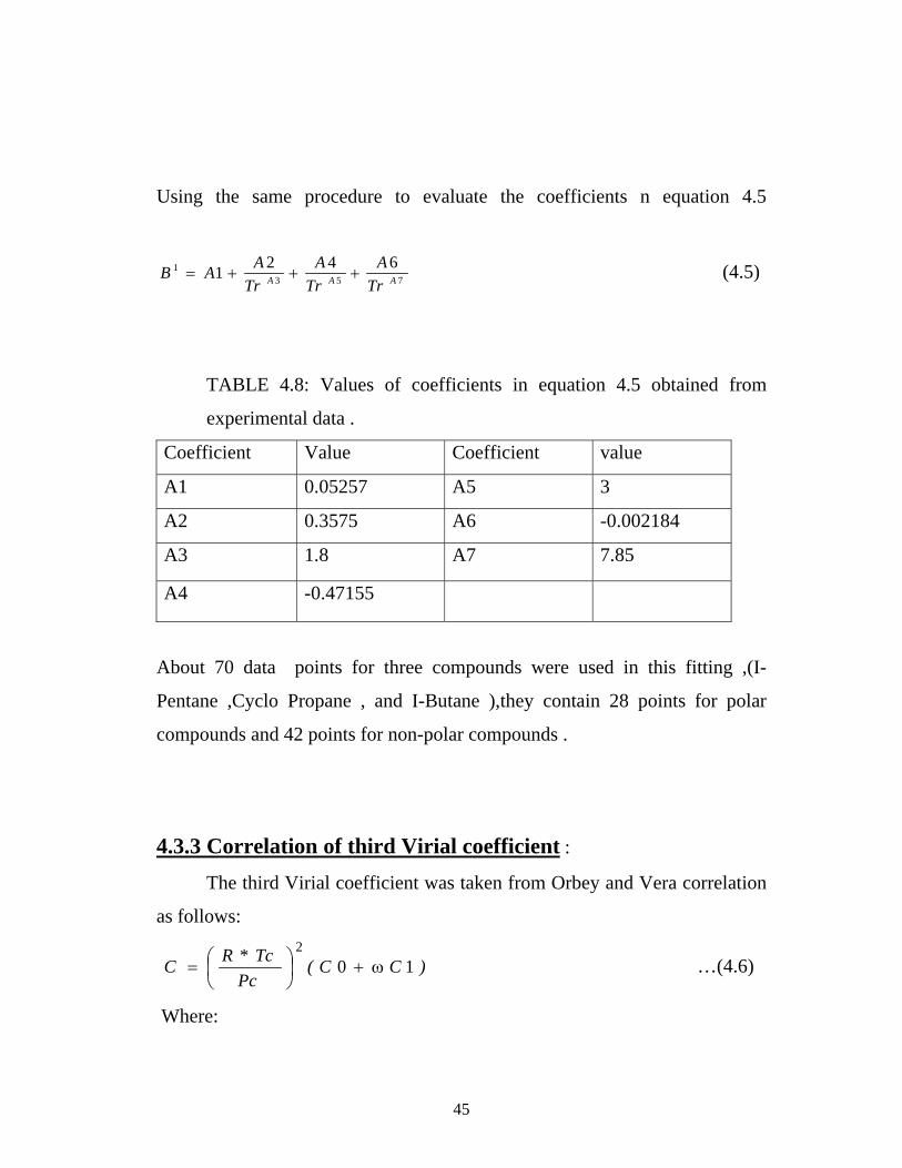
Using the same procedure to evaluate the coefficients n equation 4.5

7531 6421 AAA Tr

ATr

ATr

AAB +++= (4.5)

TABLE 4.8: Values of coefficients in equation 4.5 obtained from

experimental data .

Coefficient Value Coefficient value

A1 0.05257 A5 3

A2 0.3575 A6 -0.002184

A3 1.8 A7 7.85

A4 -0.47155

About 70 data points for three compounds were used in this fitting ,(I-

Pentane ,Cyclo Propane , and I-Butane ),they contain 28 points for polar

compounds and 42 points for non-polar compounds .

4.3.3 Correlation of third Virial coefficient : The third Virial coefficient was taken from Orbey and Vera correlation

as follows:

)CC(Pc

Tc*RC 102

ω+⎟⎠⎞

⎜⎝⎛= …(4.6)

Where:

46

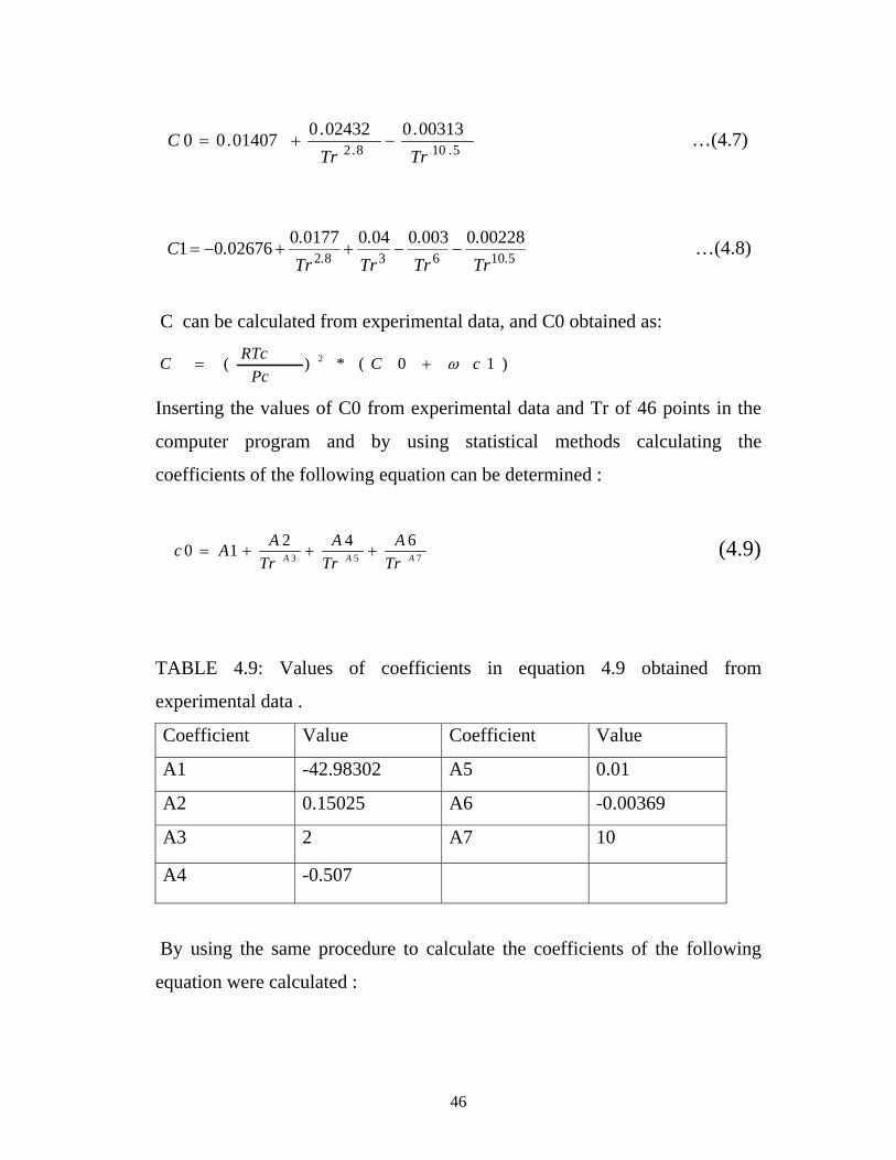
510820031300243200140700 .. Tr

.Tr..C −+= …(4.7)

51063820022800030040017700267601 .. Tr.

Tr.

Tr.

Tr..C −−++−= …(4.8)

C can be calculated from experimental data, and C0 obtained as:

)10(*)( 2 cCPc

RTcC ω+=

Inserting the values of C0 from experimental data and Tr of 46 points in the

computer program and by using statistical methods calculating the

coefficients of the following equation can be determined :

75364210 AAA Tr

ATr

ATr

AAc +++= (4.9)

TABLE 4.9: Values of coefficients in equation 4.9 obtained from

experimental data .

Coefficient Value Coefficient Value

A1 -42.98302 A5 0.01

A2 0.15025 A6 -0.00369

A3 2 A7 10

A4 -0.507

By using the same procedure to calculate the coefficients of the following

equation were calculated :

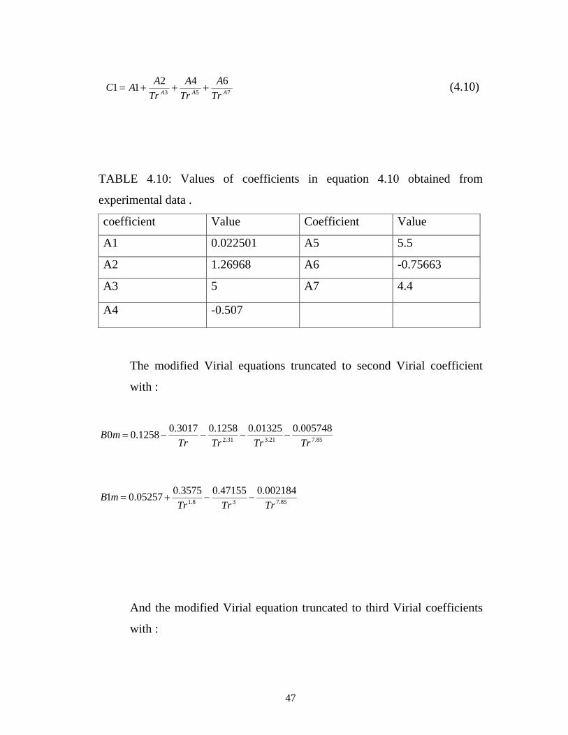
47

753

64211 AAA TrA

TrA

TrAAC +++= (4.10)

TABLE 4.10: Values of coefficients in equation 4.10 obtained from

experimental data .

coefficient Value Coefficient Value

A1 0.022501 A5 5.5

A2 1.26968 A6 -0.75663

A3 5 A7 4.4

A4 -0.507

The modified Virial equations truncated to second Virial coefficient

with :

85.721.331.2

005748.001325.01258.03017.01258.00TrTrTrTr

mB −−−−=

85.738.1

002184.047155.03575.005257.01TrTrTr

mB −−+=

And the modified Virial equation truncated to third Virial coefficients

with :

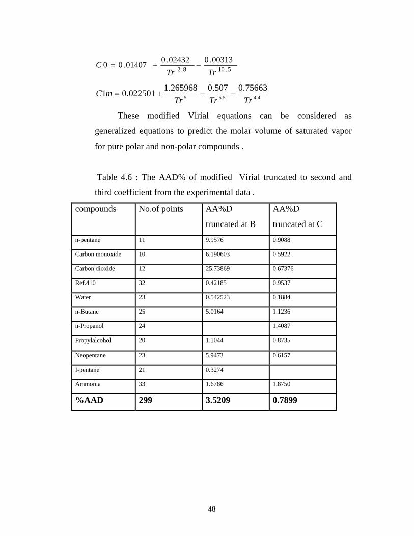
48

510820031300243200140700 .. Tr

.Tr..C −+=

4.45.55

75663.0507.0265968.1022501.01TrTrTr

mC −−+=

These modified Virial equations can be considered as

generalized equations to predict the molar volume of saturated vapor

for pure polar and non-polar compounds .

Table 4.6 : The AAD% of modified Virial truncated to second and

third coefficient from the experimental data .

compounds No.of points AA%D

truncated at B

AA%D

truncated at C

n-pentane 11 9.9576 0.9088

Carbon monoxide 10 6.190603 0.5922

Carbon dioxide 12 25.73869 0.67376

Ref.410 32 0.42185 0.9537

Water 23 0.542523 0.1884

n-Butane 25 5.0164 1.1236

n-Propanol 24 1.4087

Propylalcohol 20 1.1044 0.8735

Neopentane 23 5.9473 0.6157

I-pentane 21 0.3274

Ammonia 33 1.6786 1.8750

%AAD 299 3.5209 0.7899

49

4.4 Investigation to the mixtures : It is well known fact that the calculations of the thermodynamic

properties of the mixtures are not as easy as the calculations for pure

components. This is because of finding the critical constants that represents

the mixture from critical constants of pure components and this is done by

using what is called mixing rules . The mixing rules are not very accurate due

to difference in chemical structures of the components .Usually adjustable

parameter or parameters are needed to calculate any thermodynamic property

of mixture very accurately .

In this work the prediction of the molar volume of saturated vapors for

binary mixtures are done by using two methods :

The first method is by using Virial equation for calculating the

compressibility factor and Virial mixing rule. The second method is by using

Teja equation for calculate the compressibility factor and Virial mixing rule

the results obtained from these two methods are listed in table (4.11).

Comparison of the results obtained from the Virial mixing rule (Virial

equation truncated to second and Virial equation truncated to third coefficient

) and the results obtained fromTeja -Virial mixing rule are listed in appendix

D.The accuracy of Virial mixing rules (truncated to the third coefficient ) is

much better than that of Teja -Virial mixing rules as listed in table 4.11 .

Many developments were done in order to increase the accuracy of this

equation by using statistical program using the following form : 53 )*2exp(*4)*1exp(*21 aa ZcalxaZcalxaaZ ++=

50

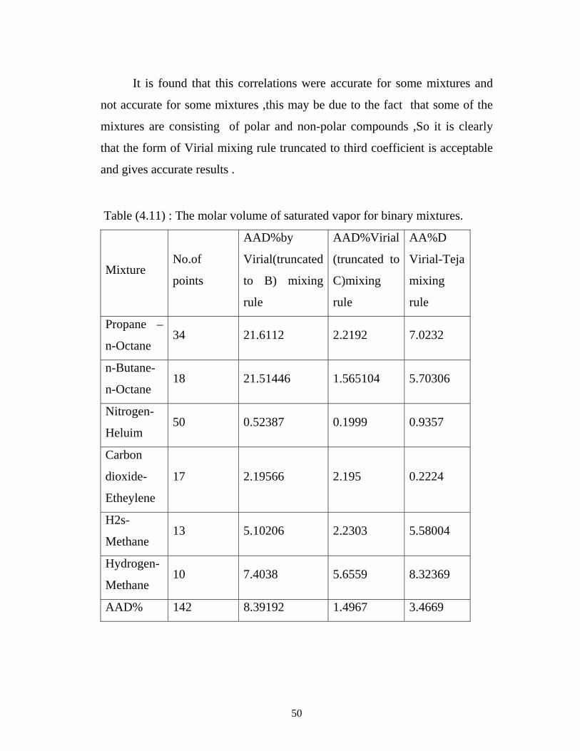
It is found that this correlations were accurate for some mixtures and

not accurate for some mixtures ,this may be due to the fact that some of the

mixtures are consisting of polar and non-polar compounds ,So it is clearly

that the form of Virial mixing rule truncated to third coefficient is acceptable

and gives accurate results .

Table (4.11) : The molar volume of saturated vapor for binary mixtures.

Mixture No.of

points

AAD%by

Virial(truncated

to B) mixing

rule

AAD%Virial

(truncated to

C)mixing

rule

AA%D

Virial-Teja

mixing

rule

Propane –

n-Octane 34 21.6112 2.2192 7.0232

n-Butane-

n-Octane 18 21.51446 1.565104 5.70306

Nitrogen-

Heluim 50 0.52387 0.1999 0.9357

Carbon

dioxide-

Etheylene

17 2.19566 2.195 0.2224

H2s-

Methane 13 5.10206 2.2303 5.58004

Hydrogen-

Methane 10 7.4038 5.6559 8.32369

AAD% 142 8.39192 1.4967 3.4669

51

CHAPTER FIVE

Discussion and Conclusions

5.1 Discussion

5.1.1 Equation of state used :

There are many equations of state that are used to calculate the molar

volume of fluids. In this research the equations of state used to calculate the

molar volume of saturated vapor of compounds were: Lee-Kesler, Redlich-

Soave, Peng-Robinson and Virial equations truncated to second and to third

terms.

Tables 5.1 and 5.2 indicate the molar volume of saturated vapor in

these moderate ranges of temperatures and pressures. The molar volume

calculated by using Lee-Kesler equation is not accurate .The AAD% is

62.432% for 3 compounds (polar and non-polar)and 72 data points .Usually

Lee-Kesler equation gives good results in superheated region and this

accuracy decreases when using this equation for saturated region .

The average percent deviation for 10 non-polar compounds of

Redlich-Soave equation and 201 data points is 18.6292 .and the AAD% is

16.1791 when using Peng-Robinson equation for 10 non-polar compounds

201 data points .On the other hand the average percent deviation for 4

compounds and 110 data points for polar compounds is 7.7664%when using

Soave equation and 7.5256% when using Peng Robinson equation . However

these two equations (Soave and Peng-Robinson) gave very accurate results

52

when they were used to calculate the molar volume of saturated vapor of

water. This is probably due to their methods of derivation. However Peng

Robinson equation can be considered better than Redlich –Soave equation to

predict the molar volume of saturated vapors.

The generalized Virial equation truncated to two terms and Virial

equation truncated to three terms are considered to be more accurate than all

the previous equations mentioned as shown in tables 5.1 and 5.2 . Virial

equation truncated to third term gave relatively better results than those

obtained from Virial equation truncated to second term.

After these comparisons one can conclude that the generalized Virial

equations truncated to second term and truncated to third term are the most

suitable equations to calculate the molar volume of saturated vapor. Thus

efforts were directed to modify these equations to increase their accuracy

(decrease the deviation from the experimental data).The average percent

deviation for 10 non-polar compounds and 201 data points is 11.8566% when

using Virial equation truncated to second term and 1.4620% for Virial

equation truncated to third term .For 4 polar compounds and 114 data points

the AAD% of Virial equation truncated to second term is 1.7645% and for

Virial equation truncated to third term is 1.1085% .Figers 5.1 to 5.7 show the

deviations from experimental data using the equations : Redlich –Soave

equation , Peng –Robinson equation ,Virial equation truncated to B and Virial

equation truncated to C after these comparison one can conclude that the

generalized Virial equation truncated to third term is the most suitable

equations to calculate the molar volume of saturated vapor. Thus efforts were

directed to modify this equation to increase its accuracy (decrease the

deviation obtained from experimental data).These figures is clearly indicate

53

that Virial equation truncated to C is the best equation for the moderate

conditions studied in this research.

Table 5.1 Comparison of the calculated molar volume obtained from different

equations for non-polar compounds. .

Compound

No.

of

points

AAD%

Lee-

Kesler

Eq.

AAD%

Redlich-

Soave

Eq.

AAD%

PR Eq.

AAD%

Virial

truncated

to B

AAD%

Virial

truncated to

C

n-Pentane 11 38.8108 18.0767 9.7192 1.318

Carbon dioxide 12 34.3104 33.0754 29.498 1.4013

Ref.410 32 0.72559 0.5528 0.2918 1.1643

Carbon

monoxide

10 17.0017 11.0508 8.5177 1.5526

n-Butane 25 15.12 15.072 15.0724 1.886

Neopentane 23 43.0845 43.0928 32.054 1.7225

Cyclopropane 28 55.1232 25.8715 26.191 9.2764 1.820

I-Pentane 21 63.8654 2.4031 1.1422 1.6678 0.8822

Ref.245 16 3.5765 1.6895 0.9497 0.9546

I-Butane 21 26.6583 24.159 11.4591

AAD% 58.8698 18.6292 16.1791 11.8566 1.4620

Table 5.2 Comparison of the calculated molar volume obtained from different

equations for polar compounds compounds No.of

points

AAD%Lee-

Kesler eq.

AAD%

Redlich-

Soave eq.

AAD%

Peng-

Robinson

eq.

AAD%Virial

eq.truncated to B

AAD%

Virial

truncated

to C

H2O 23 70.0209 0.4275 0.4414 0.1595 0.763

n-Propanol 24 5.6818 6.5217 2.7508 1.61

Propyl Alcohol 20 1.5026 1.1448 1.1945 1.25

Ammonia 47 24.448 24.3876 3.4504 0.9296

AAD% 70.0209 7.7664 7.5256 1.7645 1.1085

54

280.00 320.00 360.00 400.00 440.00T(k)

0.00

5000.00

10000.00

15000.00

20000.00

25000.00

V(cm

3/m

ole)

Experamental

Virial/C

Virial/B

Peng-Robinson

Soave

Figer 5.1 Molar volume of saturated Vapor vs.Saturated temperature for

Neopentane by using Different equations.

60.00 80.00 100.00 120.00 140.00Saturated T (K)

0.00

4000.00

8000.00

12000.00

16000.00

20000.00

V(cm

3/m

ole)

Experamental data

Virial truncated to C

Figure 5.2 Molar volume of saturated vapor vs. saturated temperature

for Carbon monoxide using Virial equation truncated to C

55

-100.00 -90.00 -80.00 -70.00 -60.00saturated T (K)

0.00

100.00

200.00

300.00

400.00

V(m

3/m

ole)

Experamental data

Virial truncated to C

Figure 5.3 Molar volume of saturated vapor vs. saturated temperature

for REF.410 using Virial equation truncated to C

240.00 280.00 320.00 360.00 400.00 440.00Saturated T (k)

0.00

5000.00

10000.00

15000.00

20000.00

25000.00

V(cm

3/m

ole)

Experamental

Virial truncated to B

Figure 5.4 Molar volume of saturated vapor vs. saturated temperature

for Carbon monoxide using Virial equation truncated to B

56

240.00 280.00 320.00 360.00 400.00 440.00Saturated T(k)

0.00

5000.00

10000.00

15000.00

20000.00

25000.00

V(cm

3/m

ole)

Experamental data

Peng-Robinson

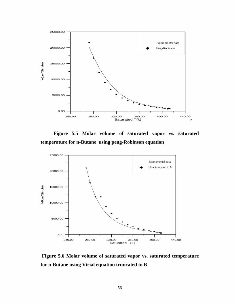
n

Figure 5.5 Molar volume of saturated vapor vs. saturated

temperature for n-Butane using peng-Robinson equation

240.00 280.00 320.00 360.00 400.00 440.00Saturated T(k)

0.00

5000.00

10000.00

15000.00

20000.00

25000.00

V9cm

3/m

ole)

Experamental data

Virial truncated to B

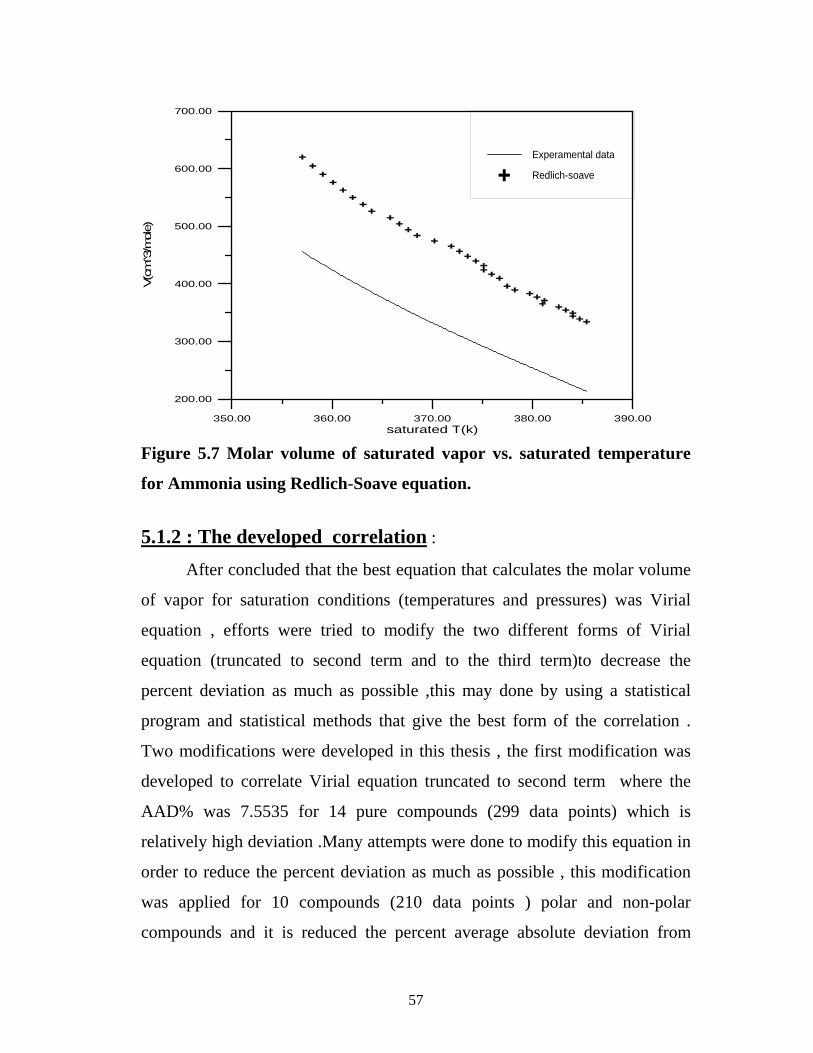
Figure 5.6 Molar volume of saturated vapor vs. saturated temperature

for n-Butane using Virial equation truncated to B

57

350.00 360.00 370.00 380.00 390.00saturated T(k)

200.00

300.00

400.00

500.00

600.00

700.00

V(cm

3/m

ole)

Experamental data

Redlich-soave

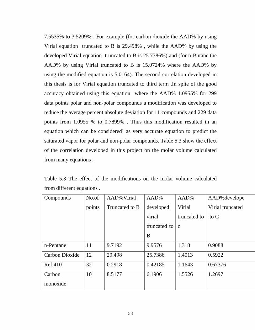
Figure 5.7 Molar volume of saturated vapor vs. saturated temperature

for Ammonia using Redlich-Soave equation.

5.1.2 : The developed correlation :

After concluded that the best equation that calculates the molar volume

of vapor for saturation conditions (temperatures and pressures) was Virial

equation , efforts were tried to modify the two different forms of Virial

equation (truncated to second term and to the third term)to decrease the

percent deviation as much as possible ,this may done by using a statistical

program and statistical methods that give the best form of the correlation .

Two modifications were developed in this thesis , the first modification was

developed to correlate Virial equation truncated to second term where the

AAD% was 7.5535 for 14 pure compounds (299 data points) which is

relatively high deviation .Many attempts were done to modify this equation in

order to reduce the percent deviation as much as possible , this modification

was applied for 10 compounds (210 data points ) polar and non-polar

compounds and it is reduced the percent average absolute deviation from

58

7.5535% to 3.5209% . For example (for carbon dioxide the AAD% by using

Virial equation truncated to B is 29.498% , while the AAD% by using the

developed Virial equation truncated to B is 25.7386%) and (for n-Butane the

AAD% by using Virial truncated to B is 15.0724% where the AAD% by

using the modified equation is 5.0164). The second correlation developed in

this thesis is for Virial equation truncated to third term .In spite of the good

accuracy obtained using this equation where the AAD% 1.0955% for 299

data points polar and non-polar compounds a modification was developed to

reduce the average percent absolute deviation for 11 compounds and 229 data

points from 1.0955 % to 0.7899% . Thus this modification resulted in an

equation which can be considered` as very accurate equation to predict the

saturated vapor for polar and non-polar compounds. Table 5.3 show the effect

of the correlation developed in this project on the molar volume calculated

from many equations .

Table 5.3 The effect of the modifications on the molar volume calculated

from different equations .

Compounds No.of

points

AAD%Virial

Truncated to B

AAD%

developed

virial

truncated to

B

AAD%

Virial

truncated to

c

AAD%develope

Virial truncated

to C

n-Pentane 11 9.7192 9.9576 1.318 0.9088

Carbon Dioxide 12 29.498 25.7386 1.4013 0.5922

Ref.410 32 0.2918 0.42185 1.1643 0.67376

Carbon

monoxide

10 8.5177 6.1906 1.5526 1.2697

59

n-Butane 25 15.0724 5.0164 1.886 1.1236

Neopentane 23 32.054 5.9473 1.7235 0.6157

Cyclopropane 28 9.2764 1.820

i-Pentane 21 1.6678 0.3274 1.6740

Ref.410 16 0.9497 0.8822 0.5061

i-Butane 21 11.4591 1.1984

Water 23 0.1595 0.5425 0.763 0.1884

n-Propanol 24 2.7508 1.61 1.4087

Propyl Alcohol 20 1.1945 1.1044 1.25 0.8735

Ammonia 47 2.9531 1.6786 0.9296 1.6785

AAD% 299 7.5535 3.5209 1.0955 0.8769

60

5.1.3 : The molar volume of saturated vapor for binary mixtures

: It is well known fact that the calculation of the thermodynamic

properties of the mixtures is not as easy as the calculation for pure

components . This is because of using the mixing rules to calculate the pseudo

critical properties and acentric factor of mixture from the critical properties

and acentric factors of pure components .Many of the mixing rules are not

quite accurate and need one or more adjustable parameters .

In this research the prediction of the saturated molar volume of binary

mixtures were done by using two methods :The first method was done by

using Virial mixing rules which is given by the following equations :

2*21*112 xx ωωω +=

2*21*112 xTcxTcTc +=

Z12=z1*x1+z2*x2

33/12

3/11 )(

8112 VcVcVc +=

2*21*112 xPcxpcPc +=

These equations were used to calculate the pseudo critical properties

and acentric factor for the mixture then using the developed Virial equation

truncated to second term and also the developed Virial equation truncated to

third term to calculate the compressibility factor of the mixtures .

61

The second method was accomplished by using the developed Virial

equation truncated to second term and the developed Virial equation truncated

to third term to calculate the compressibility factor of the mixture from the

compressibility factor of the individual component obtained at the same

reduced conditions of Tr and Pr as the mixture . The reduced conditions of the

mixture were obtained by using properties and acentric factor of the mixture .

This method is Similar to Teja [1] method for calculating the

compressibility factor of the mixture from the compressibility factors of

individual component.

Table 5.4 shows the results of deviation of saturated molar volume of

vapor for binary mixtures from experimental data using the modified Virial

equation truncated to second term and modified Virial equation truncated to

third term by the two methods motioned above .

Table 5.4 indicates the best deviation (more accuracy) are obtained

when using Virial equation truncated to third term and Virial mixing rules

.The overall average percent absolute deviation for 6 mixtures and 142 data

point is 1.4967 .

For the same 6 mixtures and 142 data point the AAD% is 3.4669

when using Virial equation truncated to third term withTeja method and

Virial mixing rules . this AAD% is increased to 8.3919 when using the

modified Virial equation truncated to second term and Virial mixing rules .

Table 5.4 indicates clearly that the best method that gives highest

accuracy (best deviation) for calculating the saturated molar volume of vapor

62

for binary mixtures is to use the modified Virial equation truncated to third

term and Virial mixing rules.

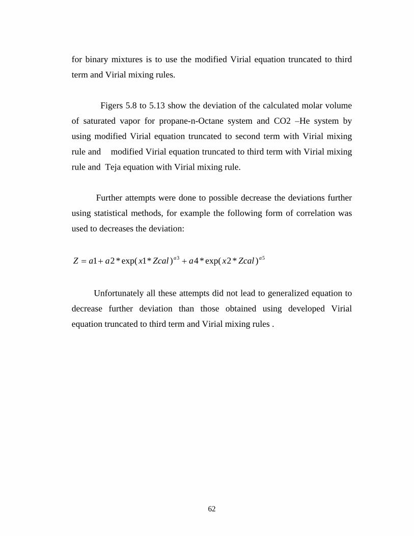
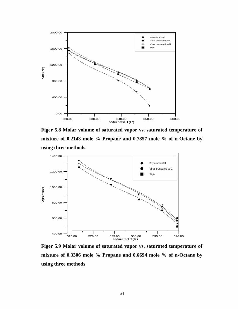
Figers 5.8 to 5.13 show the deviation of the calculated molar volume

of saturated vapor for propane-n-Octane system and CO2 –He system by

using modified Virial equation truncated to second term with Virial mixing

rule and modified Virial equation truncated to third term with Virial mixing

rule and Teja equation with Virial mixing rule.

Further attempts were done to possible decrease the deviations further

using statistical methods, for example the following form of correlation was

used to decreases the deviation:

53 )*2exp(*4)*1exp(*21 aa ZcalxaZcalxaaZ ++=

Unfortunately all these attempts did not lead to generalized equation to

decrease further deviation than those obtained using developed Virial

equation truncated to third term and Virial mixing rules .

63

Table 5.4 The AAD% of the molar volume of the saturated vapors of binary

mixtures calculated from different equations .

Mixture No.of

points

AAD%Developed

Virial

eq.(truncated to

B)with Virial

mixing rule

AAD%Developed

Virial

eq.(truncated to

C)with Virial

mixing rule

AAD%Teja

eq. with

Virial

mixing rule

Propane-

n-Octane

34 21.6112 2.2192 7.0232

n-Butane-

n-Octane

18 21.5144 1.5651 5.7031

Nitrogen-

Heluim

50 0.5238 0.1999 0.9357

Carbon

Dioxide-

ethylene

17 2.19566 2.195 0.2224

H2S-

Methane

13 5.1020 2.2303 5.5800

Hydrogen-

Methane

10 7.4038 5.6559 8.3236

AAD% 142 8.3919 3.4669 1.4967

64

520.00 530.00 540.00 550.00 560.00saturated T(R)

0.00

400.00

800.00

1200.00

1600.00

2000.00

V(ft

3/lb

)

experamental

Virial truncated to C

Virial truncated to B

Teja

Figer 5.8 Molar volume of saturated vapor vs. saturated temperature of

mixture of 0.2143 mole % Propane and 0.7857 mole % of n-Octane by

using three methods.

515.00 520.00 525.00 530.00 535.00 540.00saturated T(R)

400.00

600.00

800.00

1000.00

1200.00

1400.00

V(ft

3/m

ole)

Experamental

Virial truncated to C

Teja

Figer 5.9 Molar volume of saturated vapor vs. saturated temperature of

mixture of 0.3306 mole % Propane and 0.6694 mole % of n-Octane by

using three methods

65

470.00 480.00 490.00 500.00 510.00saturated T(R)

400.00

800.00

1200.00

1600.00

2000.00

V(ft

3/lb

)

Experamental

Virial truncated to C

Virial truncated to B

Teja

Figer 5.10 Molar volume of saturated vapor vs. saturated temperature of

mixture of 0.5729 mole % Propane and 0.4271 mole % of n-Octane by

using three methods

455.00 460.00 465.00 470.00 475.00 480.00saturated T(K)

600.00

800.00

1000.00

1200.00

1400.00

1600.00

V(cm

3/m

ole)

Experamental

Virial truncated to C

Virial truncated to B

Teja

Figer 5.11 Molar volume of saturated vapor vs. saturated

temperature of mixture of 0.8183 mole % Propane and 0.1817 mole % of

n-Octane by using three methods

66

0.00 400.00 800.00 1200.00 1600.00 2000.00saturated P (Kpa)

0.00

4.00

8.00

12.00

16.00

V(m

3/m

ole)

Experamental data

Teja

Virial truncated to C

Figer 5.12 Molar volume of saturated vapor vs. saturated temperature of

mixture of 0.119 mole % CO2 and 0.881mole % of He by using three

methods

180.00 200.00 220.00 240.00 260.00 280.00saturated T(K)

0.60

0.62

0.64

0.66

0.68

0.70

V(m

3/m

ole)

Experamental

Virial truncated to C

Virial truncated to B

Teja

Figer 5.13 Molar volume of saturated vapor vs. saturated temperature of

mixture of 0.15 mole % H2 and 0.85mole % of CH4 by using three

methods

67

5.2Conclusions :

1. There are many equations of state that can be used to calculate the

molar volume of saturated vapor .In this research and for these

moderate ranges of temperatures and pressures ,four equations of state

were used to calculate the molar volume of saturated vapor (polar and

non polar). Lee-Kesler equation was applied for 3 compounds (72 data

points including polar and non polar) with AAD% 62.432%. Redlich –

Soave equation was applied for 14 pure compounds (299 data points

polar and non-polar compounds) with AAD% 15.3125%. Peng –

Robinson equation was the third equation used to calculate the molar

volume of saturated vapor and gave AAD% 14.3476% .These three

equations proved to be unsatisfactory although the Peng-Robinson

equation gave the best deviations.

2. Truncated Virial equation used in this research, Virial equation

truncated to second term that applied for 14 compounds (299 data

points) with AAD% 7.5535, while Virial equation truncated to third

term gave AAD% is 1.0955%. It is clearly shown that for the same

compounds truncated Virial equation truncated to third term is the best

equation that can be used to calculate the molar volume of saturated

vapor and gave the lowest deviation.

....expexp

1 2 +++=V

CV

BZ

)10(* BBPc

TcRB ω+=

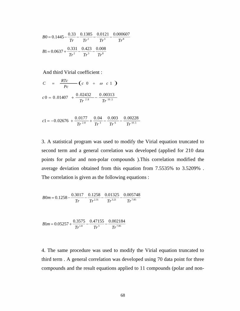
68

832

000607.00121.01385.033.01445.00TrTrTrTr

B −−−−=

832

008.0423.0331.00637.01TrTrTr

B −−+=

And third Virial coefficient :

( )10 ccPc

RTcC ω+=

5.108.200313.002432.001407.00

TrTrc −+=

5.10638.2

00228.0003.004.00177.002676.01TrTrTrTr

c −−++−=

3. A statistical program was used to modify the Virial equation truncated to

second term and a general correlation was developed (applied for 210 data

points for polar and non-polar compounds ).This correlation modified the

average deviation obtained from this equation from 7.5535% to 3.5209% .

The correlation is given as the following equations :

85.721.331.2

005748.001325.01258.03017.01258.00TrTrTrTr

mB −−−−=

85.738.1

002184.047155.03575.005257.01TrTrTr

mB −−+=

4. The same procedure was used to modify the Virial equation truncated to

third term . A general correlation was developed using 70 data point for three

compounds and the result equations applied to 11 compounds (polar and non-

69

polar ). The modified Virial equation truncated to third term reduced the

average percent absolute deviation from 1.0955 to 0.7899. The correlation is

given as the following equation:

4.45.55

75663.0507.0265968.1022501.01TrTrTr

mC −−+=

Thus the modified Virial equation truncated to the third term can be

considered as the best equation that gives the highest accuracy for prediction

the molar volume of saturated vapor .

5. For binary mixtures , the modified Virial equation truncated to second

term and truncated to third term ,with Virial mixing rule and with the

compressibility factor obtained from Teja equation. For 142 data points (6

mixtures) polar and non-polar the AAD% of the modified Virial equation

truncated to second term with Virial mixing rules is 8.39192%. While the

AAD% of modified Virial equation truncated to third term with Teja

method based on Virial mixing rule is 3.4669%. On the other hand the

AAD% for the modified Virial equation truncated to third term with Virial

mixing rules is 1.4967%. It can be considered that the modified Virial

equation truncated to third term with Virial mixing rule is the best

equation for predicting the molar volume of saturated vapor for binary

mixture.

70

5.3 Recommendations : For future work, the following recommendations can be taken in to the

consideration:

1. Applying the developed correlation for further available experimental

data at saturation conditions (polar and non-polar )

2. Applying these correlations to other thermodynamic properties like

Enthalpy , Gibbes free energy for saturated conditions .

3. Studying the possibility of applying Virial mixing rule for ternary

mixtures with an acceptable accuracy .

71

References

1. Al-Mosawe,Y.J.,"Development of Generalized correlation for determining the compressibility factor of polar compounds",M.Sc .Thesies,Alnahreen university (1995).

2. Alrawi,U.A.,"Application of truncated Virial equation for Gases at high Pressures and temperatures ",M.SC. Thesis, alnahrain university, 2002.

3. Arnold,E.W.,Lion,D.W.andEldridge,J.W, "Thermodynamic properties of Isopentane ",J.Chem and Eng.Data 10,88,April (1965) .

4. Assael,J.,Trusler,J.P.M.,andTsolakis,T.F."Thermophysiscal properties of fluid ",London and Thessaloniki , February ,1996.

5. Boyle.T.B., and Carrol,J.J.,"Calculation of acid gas density in the Vapor , liquid and Dense regions",2001 .

6. Brough,H.W.,Schlinger,W.B.,Sage,B.H.,ind.Eng.Chem.43,2442(1951).

7. Das,T.R. and Reed,C.O.and Eubank,P.T. ,"PVT surface and thermodynamic properties of n-Pentane ",J.Chem and Eng.Data ,22,1,3,(1977) .

8. Das,T.R. and Reed,C.O. Jr.and Philip, Eubank,T., "pvt surface and thermodynamic properties of isobutene ", J.Chem .Eng.Data, 18, 253, (1973).

9. Das,T.R.,Kuloor,N.R.,Indian J.Technol.,5,40(1967). 10. Davis,B.W.,Rice ,O.K.,J.Chem .Eng.,47,177(1969). 11. Douslin,B.F.,"chemical Engineering thermodynamics"MC Graw Hill

(1994). 12. Edwards,M.N.B., and Thodos,G."Prediction of saturated vapor

densities for non Polar Substance ", J.Chem and Eng. Data, vol.19, no.1 (1974).

13. Haar.L and Gallacher,J.S.,"Thermodynamic properties of Ammonia"'J.phys.Chem.Ref.Data ,Vol.7,No.3,(1978).

14. Hartono.R.,, Mansoori, G.A., "Prediction of molar volumes, vapor pressure",Published in Chem..Eng.Comm.,vol.173,p.23-24,(1999).

15. Halm,R.I., and Stiel,L.I., ,"Saturated liquid and vapor densities for polar fluids ",AICHE Journal ,Vol.16,No.1,January(1970).

72

16. Holman,J.P.,"Thermodynamics ",MC Graw-Hill Book company,Third edition ,1980.

17. Hoover,A.E.,Canfield,F.B.,Kobayashi,R,andLeland,T.W., "Determination of Virial coefficients by Burnett method " ,J.of Chem..Eng.and Eng.Data,vol.9,No.4,October (1964).

18. http://www.av8n.com/phsics/vapor.html/2003. 19. http://www.personal.ps4.edu/faculty/d/h/dhj1/classes/thermo/chapter

2.html./2002. 20. kay,W.B.,Genco,J., and Fichtner,D.A. , "Vapor liquid equilibrium

relationships of binary systems Propane-n-Octane and n-Butane n-Octane ",J.of Chem. And Eng.Data .Vol.19,No.3,1974.

21. Kesler.M.G.,and Lee,B.I.,:AICHE J.,21:510(1975) 22. Kyle,B.G.,"Chemical and process thermodynamics" secod edition

,prentice Hall international seriesin the physical and chemical sciences,1992

23. Kohn,J.P., Kurata,F.,"volumetric behavior of methane –Hydrogen Sulfied system ",J.of Chem. Eng.Data,vol.4,No.1,January (1959).

24. Lemmon,E.W.,Tjacobsen,R. ,"An equation of state for pentafluoro ethane (HFC-125) for temperatures from the triplepoint to near critical point",J.of Physical and Chemical Refrences Data,(1985).

25. Leland,T.W.,Jr.,andChappelear,P.S.,Ind.Eng.chem ,60(7) ;15 (1968) 26. link,D.C.,andKetta,J.J.,andSilberberg,L.H.,

"Thermodynamic properties of CycloPropane ", J.Chem .and Eng.Data ,16,4,416,(1971).

27. Magee,J.W., and Kobayashi,R.,"Isochoric (P,ρ ,T) measurements on (H2+CH4)at different temperatures and pressures",J.Chem Thermodynamics 18,847-858,(1986).

28. Mihajlov-DudukoVic,A.N.M.,andTasic,A.Z.,"Correlation of second Virial coefficients of polar gases by Redlich-Kowing Equation of state ", AICHE Journal ,vol 26,No 5,Page 858.

29. Moreland,M.PM,Mcketta,J.J.,and Silberberg,I.H.,"Compressibility factors and Virial coefficients of 2-Propanol",J.chem.Eng.and Eng.data ,Vol.12,No.3,July(1967).

30. Orbey,H.,and Vera,J.H.,"Correlation for the third Virial coefficient using Tc,Pcand W as parameters",AICHE J. 29,107(1983).

31. Park.K.K., ,"Comparative study on the performance of saturated vapor density correlations for pure substances", Korean Chem.Eng.Res.,Vol.42,no.1,February (2004).

73

32. Peng,D.Y.,and Robinson,D.B.,Ind.Eng.Chem.Fundam.,15:59(1976). 33. Perry,J.H.,"Chemical engineering handbook",Third edition,Mc Graw-

Hill Book company .1950. 34. prausnitz,J.M."Molecular Thermodynamics of fluid phase

equilibria,prentice Hall ,Englewood cliffs,N.J.,1969,P.(128-129). 35. Prausnitz,j.M.,and Gunn,R.D., AICHE J.,4:430,494(1958). 36. Peh ,S., and Dodge,B.F.,"Compressibility of the binary systems:

Helium-Nitrogen and Carbon dioxide – ethylene ", Journal of Chemical and Engineering Data ,vol.12,No.2,April(1967).

37. Pitzer,K.S.,D.Z.Lippman,curl.R.F.,Jr.,O.M.Huggins,and peterson,D.E.,J.Am.Chem.soc.,77,3433(1955).

38. Ramaiah,V.,and Stiel,L.I.,Ind.Eng.Chem, Process Design Develop.,11,501(1972),12:305(1973).

39. Redlich,O. and Kowing,J.N.S.,Chem.Review 44(1949)233. 40. Ried, R.C., M.prausntiz,J.M. and Poling,B.E. ,"The properties of

gases and liquid ", 4th edition, Mc Graw –Hill Book company (1989).

41. Reid,R.C.,Prausntiz,J.M., and Poling,B.E.,"properties of gases and Liquids "2001.

42. Shank,R.I.,"Thermodynamic properties of 1,1,2,2-Pentafluropropane (refrigerant 245 )", J.Chem .and Eng.Data ,12,14,474,(1967) .

43. Simth,J.M and Van Ness ,H.C.,"introduction to chemical Engineering Thermodynamics" 5th Edition,MC Graw Hill ,singapora(1996).

44. Smith,J.M.,VanNess,H.C.,and Abbott,M.M.,"Introduction to chemical engineering thermodynamics ",sixth edition ,2001.

45. Soave,G.:Chem.Eng.Sci.,27:1197(1972). 46. Thompson,P.A., and Sullivan,D. "A simple formula for saturated

vapor volume ", J.Ind.Chem.Fumdum. vol.18, no.1,(1979). 47. Thodos,R.A.W.G.,"An equation of state its application to other

substances ", AICHE Journal,Vol.3 ,No.5,May (1985). 48. Tsonpoulos ,C.,"An empirical correlation of second Virial

coefficients ",AICHhE ,20,263,(1974). 49. Valderrama,J.O., " The state of the cubic equations of state

",Ind.Eng.Chem.Res.,vol 42 ,no.8,1603-1618,(2003).

74

50. Wilding,W.V., and Rowely, R.L.Int.J.Thermophys.8,(1987)717. 51. Winnick,J.,"Chemical engineering thermodynamics", John wiely and

sons ,(1997). 52. Zemansky ,M.W.,Abott,M.M.,and Van Ness,H.C.,"Basic engineering

thermodynamics" 2nd Edition ,MC Graw Hill (1975).

APPENDIX A

PHYSICAL PROPERTIES OF THE COMPONENTS. COMPONENT M.WT Tc(k) Pc(bar) W

Zc Vc(cm3/mole)

n-pentane 72.151 469.7 33.7 0.251 0.263 304 n-butane 58.124 425.2 38 0.199 0.274 255 i-butane 58.124 408.2 36.5 0.183 0.283 263 Carbon dioxid 44.101 304.1 73.8 0.239 0.274 93.9 Ref.410 120.22 345.28 36.15 0.234 0.271 211.30 Carbon monoxide

28.010 132.9 35.0 0.066 0.295 93.2

Water 18.015 647.3 221.2 0.344 0.235 57.1 n-propanol 60.096 536.8 51.7 0.623 0.253 219 Propyl alcohol 60.096 508.3 47.6 0.665 0.248 220 Neopentane 433.8 32 0.19 Cyclopentane 42.081 379.8 54.9 0.130 0.274 163 i-pentane 70.135 511.7 45.1 0.196 0.275 260 Ref.245 134.047 685.05 456.704 0.308 0.267 291.02 Ammonia 17.031 504.5 113.5 0.250 0.244 72.5 Propane 44.094 369.8 42.5 0.153 0.244 203 Nitrogen 28.013 126.2 33.9 0.039 0.281 89.8 n-Octane 114.232 568.8 24.9 0.398 0.29 492.0 Heluim 4.003 5.19 2.27 -0.36 0.259 57.4 Ethylene 28.054 282.4 50.4 0.089 2.27 130.4 H2s 34.080 373.2 89.4 0.081 0.284 98.6 Methane 16.043 190.4 46 0.011 0.288 99.2 Hydrogen 2.016 33.2 13 -0.21 0.306 65.1

A-1

APPENDIX B

Computer program for calculating the Volume of saturated vapor . This program in QBASIC Language : CLS REM "*******************************************" REM "Computer Program for calculation the molar volume of pure compounds" REM "*******************************************" INPUT "inter the universal Gas constant R=";R INPUT "inter the critical temperature Tc="; Tc INPUT "inter the critical Pressure Pc="; Pc INPUT "inter the A centric factor w="; w INPUT "inter the Experimental Temperature T="; T INPUT "inter the Experimental pressure P="; P INPUT "inter the Experimental volume V="; V PRINT TAB(11);"*********************************" PRINT TAB (16);"RESULTS OF COMPUTER PROGRAM FOR CALCULATION OF MOLAR VOLUME OF SATURATED VAPOR FROM" PRINT TAB (32);"VIRIAL EQUATION OF STATE " PRINT TAB (11);"*********************************" PRINT TAB (1);"**--------**";TAB(16);"**----------**";TAB(33);"**--------**";TAB(51);"**-----------**";TAB(68);"**----------**" PRINTTAB (4);"Texp";TAB(19);"Pexp";TAB(25);"Vexp"; TAB(36);"Z";TAB(54);"Vcal";TAB (71);"AAD%" PRINT TAB(1) ;"**--------**";TAB(16);"**--------**";TAB(33);"**---------**";TAB(51);"**----------**";TAB(68);"**---------**"

B-1

REM"*****************************************"

REM"CALCULATION OF SECOND VIRIAL COEFFICIENT " REM "*****************************************" B0=0.1445-(0.33/(T/Tc))-(0.1385/(T/Tc)^2)-(0.0121/(T/Tc)^3)-0.000607/(T/Tc)^8) B1=0.0637+(0.331/(T/Tc)^2)-(0.423/(T/Tc)^3)-(0.008/(T/Tc)^8) B=(R*Tc/Pc)*(B0+WB1) REM"*******************************************" REM"CALCULATION OF THIRD VIRIAL COEFFICIENT" REM"******************************************" C0=0.01407+(0.02432/(T/Tc)^2.8)-(0.00313/(T/Tc)^10.5 C1=-0.02676+(0.0177/(T/Tc)^2.8)+(0.04/(T/Tc)^3-(0.003/(T/Tc)^6)-(0.00228/(T/Tc)^10.5) C=(R*Tc/Pc)^2*(c0+wc1) REM"*******************************************" REM"CALCULATION OF COMPRESSIBILITY FACTOR " REM"*******************************************" Z=1+(B/V)+(C/V^2) REM"******************************************" REM"CALCULATION OF MOLAR VOLUME " Vcal =(Z*R*T/P) PERCENT=ABS((Vexp-Vcal)/Vexp)*100 REM"*******************************************" REM "PRINT OF COMPUTER PROGRAM RESULTS" REM "*****************************************" PRINT TAB(5);"T=";T PRINT TAB(17);"P=";P PRINT TAB(32);"Vcal=";Vcal PRINT TAB (51);"PERCENT="PERCENT PRINT END

B-2

Appendix C Results of Investigation for Pure Components

TABLE(C-1) n-propanol

DEV THIS WORK

DEV VIRIAL/C

DEV VIRIAL/B

DEV PR

DEV SOAVE

VEXP(cm^3/mole)

P(bar) T(K)

3.486443.45 3.4595 3.6798 2.6265 87876.02683 298.1

2.947952.91 2.9183 3.185253.1165 64890.03711 303.1 2.124462.08 2.09183 2.471722.3621 36720.06816 313.1 1.579411.542 1.5436 2.0709 1.9039 21708.1193 323.1 1.038291.0026 1.00451 1.7095 1.4666 13380.1999 333.1 0.74188.71196 .715203 1.636371.2965 85380.3221 343.1 0.68692.6689 .6730 1.8571 1.3983 56100.5017 353.1 0.67032.672 .67800 2.1705 1.5724 37920.7575 363.1 0.74571.7766 0.7821 2.6435 1.8884 262441.113 373.1 0.84246.914 .91720 3.2136 2.2900 185761.594 383.1 1.237881.365 1.3590 4.2082 3.1091 133622.232 393.1 1.558661.7601 1.7320 5.2536 3.9859 9792 3.059 403.1 1.806632.1043 2.0324 6.3751 4.9609 7308 4.1040 413.1 1.9935 2.414 2.2626 7.632166.1059 5538 5.403 423.1 1.973142.549 2.2591 8.8954 7.3084 4260 6.991 433.1 1.763562.53 2.0126 10.24058.6570 3318 8.907 443.1 1.5988 2.6032 1.7124 12.076510.568 2064 11.189 453.1 1.128122.4071 .92960 14.010912.671 2064 13.878 463.1 0.803362.41 .02690 16.927015.853 1638 17.878 473.1 0.134132.06 1.8804 20.178419.494 1308 20.017 483.1 1.40871.61 2.7508 6.52175.681

C-1

TABLE (C-2 ) water

DEV

THIS WORK

DEV VIRIAl /C

DEVVIRIAL/

B

DEVPR

DEVSOAV

E

VEXP(cm^3

/mole)

P (mmh

g)

T(c)

.02391 .071 .1337 .0657 .0653 7627.112.15 -10

.13377 .210 .09965 .1985 .1977 3711.344.58 0

.09965 .194 .0027 .1788 .1777 2647.056.54 5 .002734 .119 .02141 .0982 .09678 1914.899.21 10 .02141 .143 .02312 .1205 .11893 1798.209.84 11 .02312 .103 .0749 .07961.0779 1688.5510.52 12 .074972 .446 .00828 .18166.1798 1585.7011.23 13 .008283 .902 .00827 .11868.1167 1491.3011.99 14 .002279 .140 .00227 .1120 .1100 1402.9612.79 15 .04246 .170 .04246 .17804.1754 1040 17.54 20 .21773 .0113 .21773 .05956.0628 782.60823.76 25 .15348 .4011 .12863 .33901.3348 594.48031.8 30 .128689 .4418 .09366 .3551 .3493 410.89847.07 37 .093662 .249 .19139 .1503 .1438 353.12955.3 40 .19139 .817 .07429 .5876 .5733 139.058149.4 60 .07429 1.123 1.1978 .6556 .6283 62.0176355.1 80 1.19782 1.592 .12219 1.965 1.9231 36.2111634.0 95 .12219 1.651

2 .1606 .87669.8338 34.9851658.0 96

.16061 1.847 .2469 .9268 .8828 32.7368707 98 .2469 1.841 .2062 1.0264.9812 31.6606733 99 .20629 1.719 .1606 .9963 .9500 30.1003760 100

.1884

.763 .1595 .4414.4275

C-2

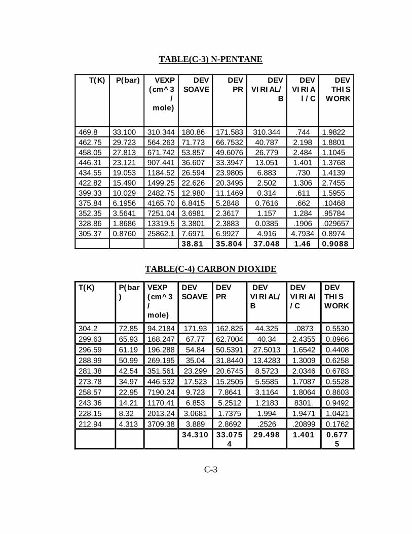
TABLE(C-3) N-PENTANE

DEVTHIS

WORK

DEV VIRIA

l /C

DEVVIRIAL/

B

DEVPR

DEVSOAVE

VEXP(cm^3

/mole)

P(bar) T(K)

1.9822 .744 310.344 171.583180.86 310.34433.100 469.8 1.8801 2.198 40.787 66.753271.773 564.26329.723 462.75 1.1045 2.484 26.779 49.607653.857 671.74227.813 458.05 1.3768 1.401 13.051 33.394736.607 907.44123.121 446.31 1.4139 .730 6.883 23.980526.594 1184.5219.053 434.55 2.7455 1.306 2.502 20.349522.626 1499.2515.490 422.82 1.5955 .611 0.314 11.146912.980 2482.7510.029 399.33 .10468 .662 0.7616 5.2848 6.8415 4165.706.1956 375.84 .95784 1.284 1.157 2.3617 3.6981 7251.043.5641 352.35 .029657.1906 0.0385 2.3883 3.3801 13319.51.8686 328.86 0.8974 4.7934 4.916 6.9927 7.6971 25862.10.8760 305.37 0.90881.46 37.048 35.80438.81

TABLE(C-4) CARBON DIOXIDE

DEV THIS WORK

DEV VIRIAl /C

DEV VIRIAL/B

DEV PR

DEV SOAVE

VEXP (cm^3/ mole)

P(bar)

T(K)

0.5530 .0873 44.325 162.825171.93 94.218472.85 304.2 0.8966 2.4355 40.34 62.700467.77 168.24765.93 299.63 0.4408 1.6542 27.5013 50.539154.84 196.28861.19 296.59 0.6258 1.3009 13.4283 31.844035.04 269.19550.99 288.99 0.6783 2.0346 8.5723 20.674523.299 351.56142.54 281.38 0.5528 1.7087 5.5585 15.250517.523 446.53234.97 273.78 0.8603 1.8064 3.1164 7.8641 9.723 7190.2422.95 258.57 0.9492 .8301 1.2183 5.2512 6.853 1170.4114.21 243.36 1.0421 1.9471 1.994 1.7375 3.0681 2013.248.32 228.15 0.1762 .20899 .2526 2.8692 3.889 3709.384.313 212.94 0.677

5 1.401 29.498 33.075

4 34.310

C-3

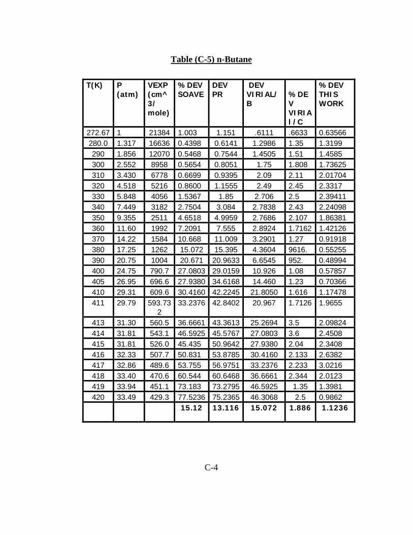
Table (C-5) n-Butane

%DEV THIS WORK

%DEV VIRIAl /C

DEV VIRIAL/ B

DEV PR

%DEV SOAVE

VEXP (cm^3/ mole)

P (atm)

T(K)

0.63566 .6633 .6111 1.151 1.003 213841 272.67 1.3199 1.35 1.2986 0.6141 0.4398 166361.317 280.0 1.4585 1.51 1.4505 0.7544 0.5468 120701.856 290 1.73625 1.808 1.75 0.8051 0.5654 8958 2.552 300 2.01704 2.11 2.09 0.9395 0.6699 6778 3.430 310 2.3317 2.45 2.49 1.1555 0.8600 5216 4.518 320 2.39411 2.5 2.706 1.85 1.5367 4056 5.848 330 2.24098 2.43 2.7838 3.084 2.7504 3182 7.449 340 1.86381 2.107 2.7686 4.9959 4.6518 2511 9.355 350 1.42126 1.7162 2.8924 7.555 7.2091 1992 11.60 360 0.91918 1.27 3.2901 11.009 10.668 1584 14.22 370 0.55255 .9616 4.3604 15.395 15.072 1262 17.25 380 0.48994 .952 6.6545 20.963320.671 1004 20.75 390 0.57857 1.08 10.926 29.015927.0803790.7 24.75 400 0.70366 1.23 14.460 34.616827.9380696.6 26.95 405 1.17478 1.616 21.8050 42.224530.4160609.6 29.31 410 1.9655 1.7126 20.967 42.840233.2376593.73

2 29.79 411

2.09824 3.5 25.2694 43.361336.6661560.5 31.30 413 2.4508 3.6 27.0803 45.576746.5925543.1 31.81 414 2.3408 2.04 27.9380 50.964245.435 526.0 31.81 415 2.6382 2.133 30.4160 53.878550.831 507.7 32.33 416 3.0216 2.233 33.2376 56.975153.755 489.6 32.86 417 2.0123 2.344 36.6661 60.646860.544 470.6 33.40 418 1.3981 1.35 46.5925 73.279573.183 451.1 33.94 419 0.9862 2.5 46.3068 75.236577.5236429.3 33.49 420 1.1236 1.886 15.072 13.11615.12

C-4

TABLE (C-6 ) CARBON MONOXIDE

DEV THIS WORK

DEV VIRIAl /C

DEV VIRIAL /B

DEV PR

DEV SOAVE

VEXP (cm^3/mole)

P(bar) T(K)

.47517 2.5710 27.2517 65.27669.865 174.85529.739 129.8 2.4145 2.5854 14.7807 51.76156.027 232.55825.53 126.5 2.4193 2.9062 9.8409 32.33 35.480 295.31121.735 123.2 2.7453 2.4575 6.6396 21.78924.273 369.13918.181 119.8 2.3245 2.5222 4.1261 16.01318.026 553.70912.696 113.2 2.3915 .7750 1.3191 8.921310.468 826.8738.4525 106.5 .66737 1.5677 1.6259 7.28688.591 1281.315.4665 99.9 1.4903 .9383 1.0635 3.86765.002 2076.413.2154 93.24 .99066 .0285 .1128 5.24673.7219 378.4331.725 86.58 .00119 .3681 .4677 3.00403.194 7593.73.814 79.92 .38056 1.2927 1.2409 2.7045.7398 17226.5.3415 73.26 1.269 1.5539 8.5777 11.0517.025

TABLE C-7 Ref.245

T(R) P (Psia)

Vexp (ft^3/lb)

DEV SOVE

DEV PR

DEV VIRIAL /B

DEV VIRIAl/C

DEV THIS work

420 5.067 870.175 0.9865 0.4331 0.5585 0.5758 0.0181 430 6.742 665.560 1.1632 0.4860 0.6007 0.6223 0.1763 440 8.841 516.239 1.3614 0.5455 0.6391 0.6651 0.2501 450 11.430 405.586 1.5844 0.6154 0.6729 0.7027 0.3356 460 14.584 322.424 1.8313 0.6957 0.7062 0.7386 0.4302 470 18.383 259.055 2.1202 0.8057 0.7270 0.7596 0.4451 480 22.910 210.245 2.4213 0.9173 0.7685 0.7974 0.5602 490 28.253 172.143 2.7787 1.0757 0.7985 0.8180 0.7692 500 34.503 142.118 3.1748 1.2652 0.8426 0.8843 0.7909 510 41.755 118.201 3.6323 1.5095 0.8929 0.8654 0.8058 520 50.656 98.972 4.1600 1.8187 0.9566 0.8842 0.8414 530 59.656 83.375 4.7694 2.2051 1.0423 0.9038 0.9191 540 70.509 70.803 5.3246 2.4182 1.3699 1.1389 1.1075 550 82.773 60.098 6.0231 3.2855 1.3103 1.9459 0.8983 560 96.559 51.358 6.8325 4.0235 1.5167 1.9711 0.7848 570 111.98 44.044 7.8471 4.9322 1.7927 1.002 0.7784 3.5006 1.6895 0.9497 0.9546 0.5061

C-5

TABLE C-8 Ref.410

T(c) P (KPa)

Vexp (m^3/ mole)

DEV SOAVE

DEV PR

DEV VIRIAl /B

DEV VIRIAL /C

DEV THIS WORK

-100 3.7 386.619 0.4969 0.4335 0.0871 0.6364 0.1473 -99 4.1 354.785 0.6119 0.6803 1.0349 0.4632 0.9738 -98 4.4 325.978 1.3656 1.2921 0.9110 1.5261 0.9748 -97 4.9 299.878 0.5067 0.5857 0.9702 0.3332 0.9060 -96 5.3 276.191 0.4284 0.3437 0.0619 0.6156 0.0043 -95 5.8 254.668 0.0734 0.0174 0.4360 0.2747 0.3686 -94 6.3 235.093 0.3474 0.2502 0.1859 0.5644 0.1170 -93 6.8 217.268 1.1436 1.0395 0.5814 1.3767 0.6522 -92 7.4 201.003 1.0039 0.8927 0.4195 1.2542 0.4914 -91 8.1 186.160 0.1620 0.0435 0.4388 0.4305 0.3664 -90 8.8 172.595 0.033 0.1594 0.6560 0.2546 0.5827 -89 9.5 160.176 0.3057 0.1711 0.3447 0.6138 0.2702 -88 10.2 148.803 1.0896 0.9463 0.4062 1.4190 0.4823 -87 11.1 138.374 0.4096 0.2574 0.2923 0.7616 0.2159 -86 12 128.800 0.2942 0.1327 0.4324 0.670 0.3553 -85 13 120.004 0.1297 0.3011 0.8779 0.2709 0.8005 -84 14 111.911 0.0544 0.2359 0.8300 0.3723 0.7521 -83 15 104.449 0.4498 0.2576 0.0156 0.9034 0.2803 -82 16.2 96.8212 0.8329 0.6279 0.7474 1.32 0.0645 -81 17.4 91.240 0.5702 0.1018 0.3252 0.6266 0.6682 -80 18.6 85.383 0.3366 0.3434 0.5845 1.1156 0.2454 -79 20 79.976 0.5283 0.0974 0.4254 0.9152 0.5047 -78 21.4 74.961 0.6167 0.2761 0.3684 1.1416 0.3455 -77 22.9 70.323 0.6390 0.3511 0.3769 1.266 0.2886 -76 24.5 66.026 1.0218 0.3595 0.0398 1.326 0.2974 -75 26.1 62.034 1.3330 0.7279 0.2421 1.3608 0.0477 -74 27.8 58.333 1.2583 0.9888 0.1364 2.1016 0.3214 -73 29.7 54.892 1.2162 0.9341 0.0624 2.069 0.2151 -72 31.7 51.684 1.4917 0.8761 0.2993 2.07 0.1405 -71 33.7 48.705 2.0563 1.1353 0.8182 2.370 0.3768 -70 35.7 45.928 1.5069 1.6828 0.2464 2.300 0.8953 -69 38.2 43.344 1.4586 1.1162 0.2254 2.500 0.3222 0.7255 0.552 0.2918 1.1643 0.6737

C-6

TABLE C-9 Propyl Alcohol

T(R) P (Psia)

Vexp (ft^3/lb)

DEV SOVE

DEV PR

DEV VIRIAL /B

DEV VIRIAl/C

DEV THIS work

501 0.0890 60113.4 0.4766 0.476 0.4475 0.447 0.476511 0.1358 40175.4 0.5029 0.50206 0.4644 0.4644 0.502521 0.2032 27363.0 0.5256 0.5243 0.4754 0.475 0.525531 0.2986 18970.2 0.5578 0.555 0.4930 0.493 0.557

541 0.4313 13372.8 0.6027 0.600 0.5212 0.521 0.602551 0.6131 9576 0.6597 0.65 0.5579 0.557 0.659561 0.8582 6959.4 0.7293 0.72 0.6036 0.6035 0.729571 1.1841 5128.14 0.8187 0.812 0.6653 0.665 0.818581 1.6115 3828.66 0.9300 0.912 0.7447 0.744 0.830591 2.165 2893.92 1.0602 1.0496 0.8387 0.8386 1.060601 2.8735 2212.98 1.2143 1.2005 0.9520 0.9518 1.114611 3.76 1710.9 1.3934 1.375 1.0856 1.058 1.093621 4.891 1336.44 1.6035 1.5814 1.245 1.245 1.035631 6.2812 1054.2 1.8432 1.815 1.4293 1.429 1.243641 7.9861 839.22 2.118 2.084 1.643 1.643 1.118651 10.059 673.86 2.4309 2.388 1.8900 1.883 1.359661 12.556 545.712 2.7551 2.7037 2.142 2.14 1.525668 14.696 469.452 3.0236 2.9643 2.3526 2.35 1.023671 15.54 445.08 3.1833 3.12104 2.49 2.49 1.183681 19.078 365.76 3.624 3.5498 2.85005 2.85 1.624

1.502 1.1448 1.1945 1.25 0.95

C-7

TABLE C-10 Neopentane

T(K) P (atm)

Vexp (cm^3/mole)

DEV SOAVE

DEV PR

DEV VIRIAL /B

DEV VIRIAL /C

DEV THIS work

282.6 1 22103 1.4408 0.9716 0.8979 0.9510 0.8369290 1.295 17265 2.1341 1.6177 0.5043 0.5620 0.4463300 1.797 12670 2.552 1.9900 0.4984 0.5530 0.4298310 2.434 9490 3.0625 2.4802 0.4870 0.5243 0.3808320 3.227 7234 3.6870 3.1100 0.488 0.481 0.3026330 4.199 5597 4.4368 3.9210 0.5430 0.4509 0.2172340 5.373 4385 5.371 4.9501 0.6659 0.4265 0.1135350 6.773 3472 6.5281 6.2622 0.9103 0.4301 0.0082360 8.425 2772 7.995 7.9390 1.3258 0.4640 0.0999370 10.357 2226 9.907 10.126 1.9830 0.5243 0.2246380 12.596 1794 11.934 13.000 3.0133 0.6190 0.3646390 15.176 1446 14.953 16.870 4.644 0.7570 0.5249400 18.134 1161 19.055 22.186 7.342 0.9880 0.6748410 21.513 920 24.708 30.196 12.062 1.2780 0.8885415 23.377 809.6 33.237 36.147 15.958 1.4330 1.0569420 25.336 706.9 39.563 43.959 21.742 1.6440 1.2247425 27.489 603.6 47.851 55.282 31.833 2.1901 1.1386426 27.931 583.4 59.868 58.095 34.614 2.3322 1.0953427 28.380 561.9 62.847 61.524 37.9985 2.4710 1.0644428 28.834 540.6 66.465 65.212 41.8682 2.651 1.0042429 29.294 517.5 70.363 69.843 46.7895 2.8226 0.9455430 29.758 493.2 75.238 75.400 52.9755 3.0276 0.8600431 30.232 466.9 81.076 82.330 61.1808 3.2923 0.7104432 30.711 436.7 88.345 91.850 73.1933 4.1833 0.4748433 31.195 387.5 106.55 112.80 102.105 3.6241 0.1209433.5 31.442 366.4 116.63 123.25 119.226 4.3697 0.4614433.7 31.545 311 154.38 162.19 90.6239 3.4713 0.9533 43.084 43.09 32.054 1.722 0.615

C-8

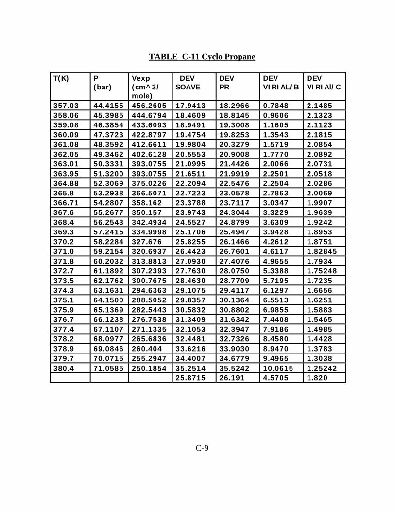
TABLE C-11 Cyclo Propane

T(K) P (bar)

Vexp (cm^3/ mole)

DEV SOAVE

DEV PR

DEV VIRIAL/B

DEV VIRIAl/C

357.03 44.4155 456.2605 17.9413 18.2966 0.7848 2.1485 358.06 45.3985 444.6794 18.4609 18.8145 0.9606 2.1323 359.08 46.3854 433.6093 18.9491 19.3008 1.1605 2.1123 360.09 47.3723 422.8797 19.4754 19.8253 1.3543 2.1815 361.08 48.3592 412.6611 19.9804 20.3279 1.5719 2.0854 362.05 49.3462 402.6128 20.5553 20.9008 1.7770 2.0892 363.01 50.3331 393.0755 21.0995 21.4426 2.0066 2.0731 363.95 51.3200 393.0755 21.6511 21.9919 2.2501 2.0518 364.88 52.3069 375.0226 22.2094 22.5476 2.2504 2.0286 365.8 53.2938 366.5071 22.7223 23.0578 2.7863 2.0069 366.71 54.2807 358.162 23.3788 23.7117 3.0347 1.9907 367.6 55.2677 350.157 23.9743 24.3044 3.3229 1.9639 368.4 56.2543 342.4934 24.5527 24.8799 3.6309 1.9242 369.3 57.2415 334.9998 25.1706 25.4947 3.9428 1.8953 370.2 58.2284 327.676 25.8255 26.1466 4.2612 1.8751 371.0 59.2154 320.6937 26.4423 26.7601 4.6117 1.82845 371.8 60.2032 313.8813 27.0930 27.4076 4.9655 1.7934 372.7 61.1892 307.2393 27.7630 28.0750 5.3388 1.75248 373.5 62.1762 300.7675 28.4630 28.7709 5.7195 1.7235 374.3 63.1631 294.6363 29.1075 29.4117 6.1297 1.6656 375.1 64.1500 288.5052 29.8357 30.1364 6.5513 1.6251 375.9 65.1369 282.5443 30.5832 30.8802 6.9855 1.5883 376.7 66.1238 276.7538 31.3409 31.6342 7.4408 1.5465 377.4 67.1107 271.1335 32.1053 32.3947 7.9186 1.4985 378.2 68.0977 265.6836 32.4481 32.7326 8.4580 1.4428 378.9 69.0846 260.404 33.6216 33.9030 8.9470 1.3783 379.7 70.0715 255.2947 34.4007 34.6779 9.4965 1.3038 380.4 71.0585 250.1854 35.2514 35.5242 10.0615 1.25242 25.8715 26.191 4.5705 1.820

C-9

TABLE C-12 I-Pentane

T(R) P (psia)

Vexp (ft^3/lb)

DEV SOAVE

DEV PR

DEV VIRIAL/B

DEV VIRIAl/C

460 2.18 2236.62 0.5603 0.2584 0.7932 0.8073 470 2.87 1715.85 0.6746 0.3035 0.8511 0.8695 480 3.73 1343.05 0.7976 0.3474 0.9106 0.9342 490 4.78 1065.27 0.8827 0.3442 1.0123 1.0418 500 6.05 854.779 1.0179 0.3815 1.0733 1.1093 510 7.59 691.286 1.2254 0.4793 1.0805 1.1238 520 9.42 564.634 1.3879 0.5230 1.1396 1.1903 530 11.57 465.5956 1.6459 0.6528 1.1199 1.1780 540 14.12 386.050 1.6024 0.4731 1.3974 1.4623 550 17.06 322.975 1.9491 0.6727 1.3300 1.4011 560 20.46 271.993 2.0581 0.6297 1.4970 1.5723 570 24.35 230.589 2.2757 0.6897 1.5870 1.6638 580 28.79 196.548 2.6359 0.8802 1.5808 1.6559 590 33.86 168.449 1.7735 0.1346 2.6556 2.7217 600 39.46 145.3154 2.7496 1.1760 2.1770 2.2308 610 45.77 125.8325 3.7728 1.3133 1.9892 2.0215 620 52.84 109.4002 4.4821 1.8283 2.1766 2.1762 630 60.72 95.3860 4.2956 1.4672 2.1185 2.0715 640 69.49 85.859 5.3641 2.3240 2.8270 2.7183 650 79.20 75.037 5.8596 2.6203 2.6679 2.4724 660 89.92 66.1625 5.4875 5.8596 3.0397 2.7328 2.4031 1.1422 1.6678 1.6740

C-10

TABLE C-13 Ammonia

T(k) P(atm) Vexp (cm^3/ mole)

DEV SOAVE

DEV PR

DEV VIRIAL /B

DEV VIRIAl/C

DEV This work

357.03 44.4115 456.260 15.283 15.4402 0.0966 2.1485 2.1070358.06 45.398 444.679 16.1255 15.9190 0.0023 2.1323 2.1439359.08 46.385 423.609 16.5784 16.3762 0.1449 2.1123 2.1426360.09 47.372 422.879 16.9818 16.8753 0.2781 2.1081 2.1509361.09 48.359 412.661 17.4051 17.3253 0.4474 2.0853 2.1421362.05 49.346 402.612 17.8885 17.7953 0.6186 2.0891 2.1306363.09 50.333 393.075 18.3275 18.3275 0.7708 2.0730 2.1485363.95 51.3200 391.755 18.7645 18.8145 0.9606 2.0518 2.1323365.8 53.2938 366.507 19.2395 19.3008 1.1605 2.0006 2.1123366.71 54.2807 358.162 19.6919 19.8253 1.3543 1.9907 2.1081367.6 55.2677 350.153 20.7048 20.3279 1.5719 1.9639 2.0891368.48 56.2546 342.493 21.2026 20.9008 1.7770 1.9242 2.0730370.21 58.2284 327.676 21.7061 21.4426 2.0066 1.8751 2.0518371.05 59.2154 320.693 22.2091 21.9919 2.2501 1.8284 2.0286371.89 60.2023 313.818 22.7634 22.5476 2.5041 1.7934 2.0006372.71 61.1892 307.239 23.3023 23.10354 2.7711 1.7542 1.9907372.71 62.1761 300.767 23.8235 23.7117 3.0347 1.7234 1.9639373.53 63.1630 294.636 24.3832 24.3044 3.3229 1.6656 1.9242374.34 64.1500 288.505 24.9790 24.8799 3.6309 1.6250 1.8952375.13 65.1369 282.544 26.1272 25.4947 3.9428 1.5882 1.8751375.92 66.1238 276.753 26.7375 26.1466 4.2612 1.5465 1.7934376.7 67.1107 271.133 27.3747 27.4076 4.9655 1.4984 1.7542377.47 68.0977 265.683 27.9570 28.0756 5.3388 1.4428 1.7234378.23 70.0715 255.294 28.6223 28.7709 5.7195 1.3038 1.6656379.72 71.0584 2501.18 29.3055 29.4117 5.8325 1.2524 1.6250380.72 72.0454 245.246 29.9982 30.1364 5.9923 1.1889 1.5882381.19 73.0323 2403.37 30.6969 30.8802 6.0276 1.1380 1.5465381.0 74.0192 235.538 31.3980 31.6342 6.4645 1.0729 1.4984382.62 75.0061 230.940 32.0977 32.3947 6.8023 0.9929 1.4428383.32 75.9931 226.512 32.7922 33.1581 7.0135 0.9056 1.3783384.02 76.9800 222.084 33.5733 33.7251 7.2432 0.8269 1.3038384.71 77.9669 217.656 33.8251 34.0251 7.6758 0.7639 1.2524385.40 78.9538 213.398 34.0221 34.3251 7.8805 0.6744 1.6425AAD% 24.448 24.3876 3.4504 0.929 1.875

C-11

TABLE C-14 i-Butane

T(k) P (atm)

Vexp (cm^3/mole)

DEV SOAVE

DEV PR

DEV VIRIAL /B

DEV VIRIAl/C

261.32 1 20682 0.7373 0.1101 0.0023 1.69852 270 1.39 15202 1.0312 0.2837 0.1449 1.7669 280 1.968 10921 1.8747 0.9314 0.2781 1.4371 290 2.714 8032 2.7049 1.6787 0.4474 1.2136 300 3.656 6031 3.5274 2.3716 0.6186 1.1166 310 4.826 4615 4.2171 2.9428 0.7708 1.2803 320 6.254 3577 5.2443 3.8573 0.9606 1.3619 330 7.975 2801 6.6687 5.1685 1.1605 1.3971 340 10.02 2209 8.7409 7.1161 1.3543 1.3050 350 12.44 1750 11.4798 9.7014 1.5719 1.2441 360 15.25 1387 15.5541 13.5686 1.7770 0.9788 370 18.52 1094 21.3483 19.0582 2.0066 0.7173 380 22.28 849.7 30.5465 27.7788 2.2501 0.3129 385 24.36 745.3 36.4548 33.3594 2.5041 0.3541 390 26.59 647.6 44.2023 40.6772 2.7711 0.5263 395 28.97 556.1 54.4850 50.3904 3.0347 0.9735 396 29.46 539.1 56.7822 52.5580 3.3229 1.1187 397 29.96 521.6 59.4119 55.0433 3.6309 1.2725 398 30.47 505.3 61.8717 57.3570 3.9428 1.4881 399 30.98 488.2 64.8632 60.1855 4.2612 1.6767 400 31.51 471 68.0776 63.2189 4.9655 1.9272 26.6582 24.1598 1.9579 1.1984

C-12

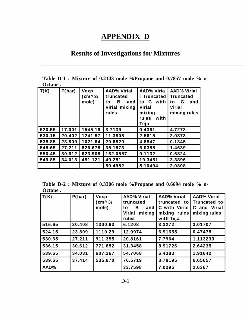
APPENDIX D

Results of Investigations for Mixtures Table D-1 : Mixture of 0.2143 mole %Propane and 0.7857 mole % n-Octane .

T(K) P(bar) Vexp (cm^3/ mole)

AAD%Virial truncated to B and Virial mixing rules

AAD%Virial truncated to C with Virial mixing rules with Teja

AAD%Virial Truncated to C and Virial mixing rules

520.55 17.001 1545.19 3.7139 0.4361 4.7273 530.15 20.402 1241.57 11.3808 2.5615 2.0873 538.85 23.809 1021.64 20.6820 4.8847 0.1345 545.65 27.211 826.678 35.1573 6.0385 1.4639 550.45 30.612 623.908 162.0557 9.1132 0.6824 549.85 34.013 451.121 49.251 19.3451 3.3896 50.4982 5.10494 2.0808 Table D-2 : Mixture of 0.3306 mole %Propane and 0.6694 mole % n-Octane . T(K) P(bar) Vexp

(cm^3/ mole)

AAD%Virial truncated to B and Virial mixing rules

AAD%Virial truncated to C with Virial mixing rules with Teja

AAD%Virial Truncated to C and Virial mixing rules

516.65 20.408 1300.63 6.1208 3.3272 3.01707

524.15 23.809 1110.29 12.9974 6.91655 0.47478 530.65 27.211 911.355 20.8161 7.7964 1.113233 536.15 30.612 771.652 31.3458 8.91726 2.64235

539.65 34.031 607.367 54.7068 6.4383 1.91642 539.65 37.414 535.870 76.5719 8.78195 6.65657 AAD% 33.7598 7.0295 2.6367

D-1

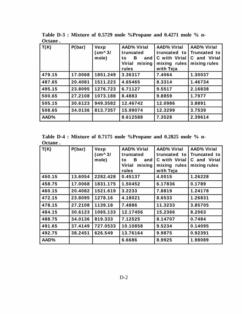
Table D-3 : Mixture of 0.5729 mole %Propane and 0.4271 mole % n-Octane . T(K) P(bar) Vexp

(cm^3/ mole)

AAD%Virial truncated to B and Virial mixing rules

AAD%Virial truncated to C with Virial mixing rules with Teja

AAD%Virial Truncated to C and Virial mixing rules

479.15 17.0068 1851.249 3.36317 7.4064 1.30037

487.65 20.4081 1511.223 4.65465 8.3314 1.46734 495.15 23.8095 1276.723 6.71127 9.5517 2.16838 500.65 27.2108 1073.188 8.4883 9.8859 1.7977

505.15 30.6123 949.3582 12.46742 12.0986 3.8891 508.65 34.0136 813.7357 15.99074 12.3299 3.7539 AAD% 8.612588 7.3528 2.39614

Table D-4 : Mixture of 0.7175 mole %Propane and 0.2825 mole % n-Octane . T(K) P(bar) Vexp

(cm^3/ mole)

AAD%Virial truncated to B and Virial mixing rules

AAD%Virial truncated to C with Virial mixing rules with Teja

AAD%Virial Truncated to C and Virial mixing rules

450.15 13.6054 2282.428 0.45137 4.0015 1.26228

458.75 17.0068 1831.175 1.50452 6.17836 0.1789 460.15 20.4082 1521.619 3.2233 7.8819 1.24178 472.15 23.8095 1278.16 4.18021 8.6533 1.26831

478.15 27.2108 1139.18 7.4886 11.3233 3.85705 484.15 30.6123 1065.133 12.17456 15.2366 8.2063 488.75 34.0136 819.333 7.12525 8.14707 0.7484 491.65 37.4149 727.0533 10.10858 9.5234 0.14095 492.75 38.2451 626.549 13.76164 9.9875 0.92391 AAD% 6.6686 8.9925 1.98089

D-2

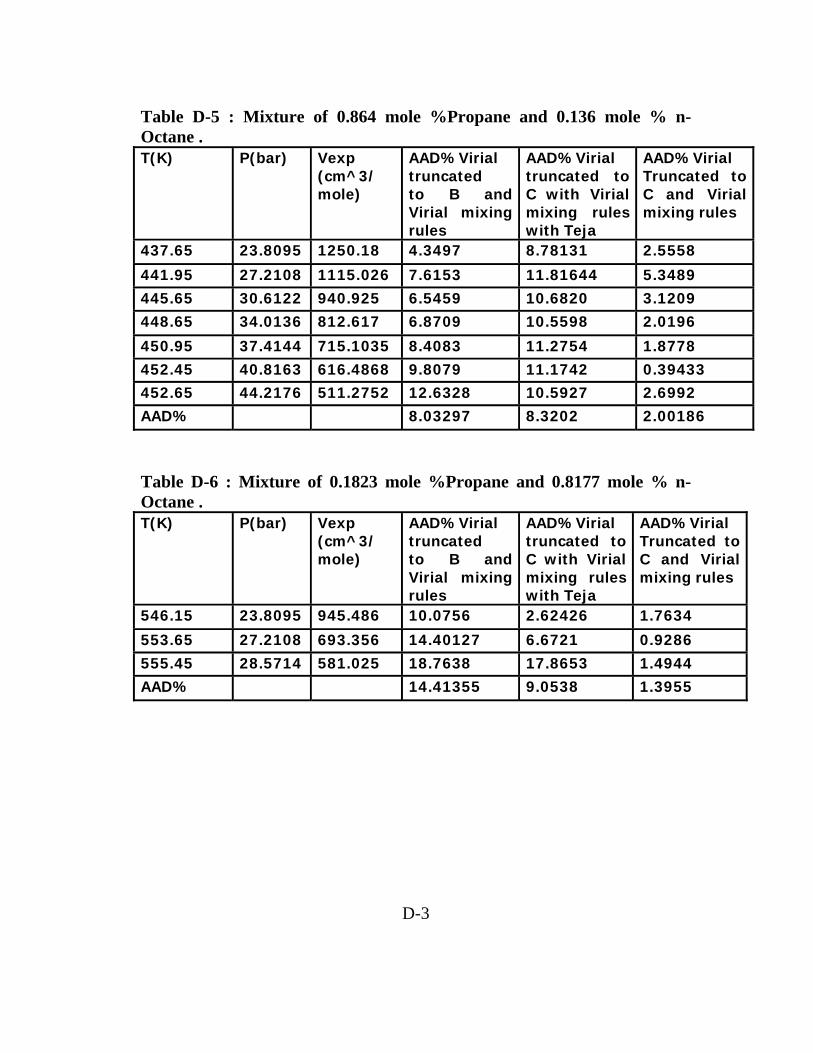
Table D-5 : Mixture of 0.864 mole %Propane and 0.136 mole % n-Octane . T(K) P(bar) Vexp

(cm^3/ mole)

AAD%Virial truncated to B and Virial mixing rules

AAD%Virial truncated to C with Virial mixing rules with Teja

AAD%Virial Truncated to C and Virial mixing rules

437.65 23.8095 1250.18 4.3497 8.78131 2.5558

441.95 27.2108 1115.026 7.6153 11.81644 5.3489 445.65 30.6122 940.925 6.5459 10.6820 3.1209 448.65 34.0136 812.617 6.8709 10.5598 2.0196

450.95 37.4144 715.1035 8.4083 11.2754 1.8778 452.45 40.8163 616.4868 9.8079 11.1742 0.39433 452.65 44.2176 511.2752 12.6328 10.5927 2.6992 AAD% 8.03297 8.3202 2.00186

Table D-6 : Mixture of 0.1823 mole %Propane and 0.8177 mole % n-Octane . T(K) P(bar) Vexp

(cm^3/ mole)

AAD%Virial truncated to B and Virial mixing rules

AAD%Virial truncated to C with Virial mixing rules with Teja

AAD%Virial Truncated to C and Virial mixing rules

546.15 23.8095 945.486 10.0756 2.62426 1.7634

553.65 27.2108 693.356 14.40127 6.6721 0.9286 555.45 28.5714 581.025 18.7638 17.8653 1.4944 AAD% 14.41355 9.0538 1.3955

D-3

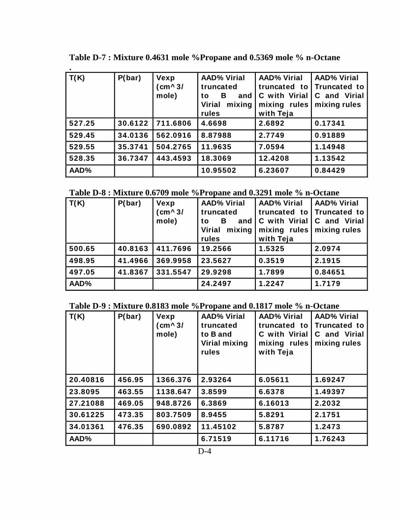
Table D-7 : Mixture 0.4631 mole %Propane and 0.5369 mole % n-Octane . T(K) P(bar) Vexp

(cm^3/ mole)

AAD%Virial truncated to B and Virial mixing rules

AAD%Virial truncated to C with Virial mixing rules with Teja

AAD%Virial Truncated to C and Virial mixing rules

527.25 30.6122 711.6806 4.6698 2.6892 0.17341

529.45 34.0136 562.0916 8.87988 2.7749 0.91889 529.55 35.3741 504.2765 11.9635 7.0594 1.14948 528.35 36.7347 443.4593 18.3069 12.4208 1.13542

AAD% 10.95502 6.23607 0.84429

Table D-8 : Mixture 0.6709 mole %Propane and 0.3291 mole % n-Octane T(K) P(bar) Vexp

(cm^3/ mole)

AAD%Virial truncated to B and Virial mixing rules

AAD%Virial truncated to C with Virial mixing rules with Teja

AAD%Virial Truncated to C and Virial mixing rules

500.65 40.8163 411.7696 19.2566 1.5325 2.0974

498.95 41.4966 369.9958 23.5627 0.3519 2.1915 497.05 41.8367 331.5547 29.9298 1.7899 0.84651 AAD% 24.2497 1.2247 1.7179

Table D-9 : Mixture 0.8183 mole %Propane and 0.1817 mole % n-Octane T(K)

P(bar) Vexp (cm^3/ mole)

AAD%Virial truncated to B and Virial mixing rules

AAD%Virial truncated to C with Virial mixing rules with Teja

AAD%Virial Truncated to C and Virial mixing rules

20.40816 456.95 1366.376 2.93264 6.05611 1.69247

23.8095 463.55 1138.647 3.8599 6.6378 1.49397 27.21088 469.05 948.8726 6.3869 6.16013 2.2032 30.61225 473.35 803.7509 8.9455 5.8291 2.1751

34.01361 476.35 690.0892 11.45102 5.8787 1.2473

AAD% 6.71519 6.11716 1.76243

D-4

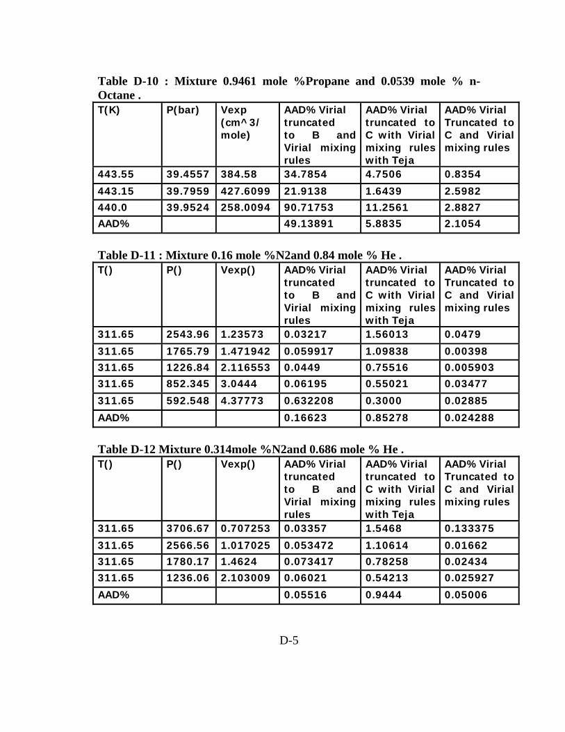
Table D-10 : Mixture 0.9461 mole %Propane and 0.0539 mole % n-Octane . T(K) P(bar) Vexp

(cm^3/ mole)

AAD%Virial truncated to B and Virial mixing rules

AAD%Virial truncated to C with Virial mixing rules with Teja

AAD%Virial Truncated to C and Virial mixing rules

443.55 39.4557 384.58 34.7854 4.7506 0.8354

443.15 39.7959 427.6099 21.9138 1.6439 2.5982 440.0 39.9524 258.0094 90.71753 11.2561 2.8827 AAD% 49.13891 5.8835 2.1054

Table D-11 : Mixture 0.16 mole %N2and 0.84 mole % He . T() P() Vexp() AAD%Virial

truncated to B and Virial mixing rules

AAD%Virial truncated to C with Virial mixing rules with Teja

AAD%Virial Truncated to C and Virial mixing rules

311.65 2543.96 1.23573 0.03217 1.56013 0.0479

311.65 1765.79 1.471942 0.059917 1.09838 0.00398 311.65 1226.84 2.116553 0.0449 0.75516 0.005903 311.65 852.345 3.0444 0.06195 0.55021 0.03477

311.65 592.548 4.37773 0.632208 0.3000 0.02885

AAD% 0.16623 0.85278 0.024288

Table D-12 Mixture 0.314mole %N2and 0.686 mole % He . T() P() Vexp() AAD%Virial

truncated to B and Virial mixing rules

AAD%Virial truncated to C with Virial mixing rules with Teja

AAD%Virial Truncated to C and Virial mixing rules

311.65 3706.67 0.707253 0.03357 1.5468 0.133375

311.65 2566.56 1.017025 0.053472 1.10614 0.01662 311.65 1780.17 1.4624 0.073417 0.78258 0.02434 311.65 1236.06 2.103009 0.06021 0.54213 0.025927

AAD% 0.05516 0.9444 0.05006

D-5

Table D-13: Mixture of 0.564 mole %N2 and 0.436 mole % He T()

P() Vexp() AAD%Virial truncated to B and Virial mixing rules

AAD%Virial truncated to C with Virial mixing rules with Teja

AAD%Virial Truncated to C and Virial mixing rules

311.6 4301.34 0.61537 0.8138 0.4149 0.7711

311.6 3167.52 0.8306 0.5512 0.3103 0.5198 311.6 2337.26 1.1212 0.4024 0.2085 0.3794 311.6 1726.18 1.5133 0.2889 0.1484 0.2720

311.6 1276.18 2.0426 0.2096 0.1060 0.1972 311.6 943.943 2.7523 0.1516 0.0776 0.1425 311.6 698.534 3.7216 0.1156 0.0527 0.1077 311.6 517.061 5.0235 0.0845 0.0381 0.0794 311.6 383.008 6.7807 0.1115 0.0215 0.1078 AAD% 0.3032 2.6636 0.2863

Table D-14 : Mixture of 0.178 mole %N2 and 0.822 mole % He T()

P() Vexp() AAD%Virial truncated to B and Virial mixing rules

AAD%Virial truncated to C with Virial mixing rules with Teja

AAD%Virial Truncated to C and Virial mixing rules

373.15 4425.87 0.7103 0.3421 1.4645 0.4495

373.15 3265.09 0.9585 0.1557 1.1468 0.2359 373.15 2411.94 1.2936 0.0362 0.9087 0.0959 373.15 1783.32 1.7459 0.0421 0.7311 0.0023

373.15 1319.45 2.3561 0.0881 0.5925 0.0551 373.15 976.773 3.1800 0.0971 0.4673 0.0726 373.15 723.15 4.2915 0.0991 0.3715 0.0899 373.15 535.907 5.7911 0.0839 0.2846 0.0704 AAD% 0.1057 0.7815 0.1328

D-6

Table D-15 : Mixture of 0.86 mole %N2 and 0.14 mole % He T()

P() Vexp() AAD%Virial truncated to B and Virial mixing rules

AAD%Virial truncated to C with Virial mixing rules with Teja

AAD%Virial Truncated to C and Virial mixing rules

311.65 4245.51 0.6240 1.6753 0.4141 1.5507

311.65 3127.19 0.8373 0.6600 0.2455 0.5663 311.65 2307.27 1.1369 0.9347 0.2944 0.8659 311.65 1703.88 1.5346 0.6921 0.2300 0.6410

311.65 1259.36 2.0713 0.5143 0.1787 0.4764 311.65 931.58 2.7959 0.4044 0.1596 0.3763 311.65 689.31 3.7740 0.3123 0.1329 0.291 311.65 510.17 5.0941 0.2357 0.1040 0.2203 AAD% 0.6786 0.2199 0.6236

Table D-16 : Mixture of 0.513 mole %N2 and 0.487 mole % He T()

P() Vexp() AAD%Virial truncated to B and Virial mixing rules

AAD%Virial truncated to C with Virial mixing rules with Teja

AAD%Virial Truncated to C and Virial mixing rules

373.15 4388.58 0.7201 0.5986 0.8859 0.3883

373.15 3233.78 0.9718 0.8095 0.6992 0.2099 373.15 23869.6 1.3116 1.0939 0.5636 0.0905 373.15 1763.35 1.7701 1.477 0.4586 0.0153

373.15 1303.74 2.3889 1.9957 0.3958 0.0507 373.15 964.816 3.2240 2.6938 0.3168 0.0644 373.15 714.239 4.3508 3.6360 0.2612 0.0761 373.15 528.916 5.8716 4.9071 0.2121 0.0759 AAD% 2.1515 0.5007 0.1214

D-7

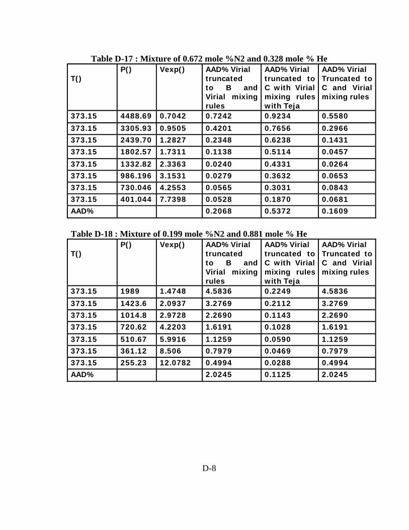
Table D-17 : Mixture of 0.672 mole %N2 and 0.328 mole % He T()

P() Vexp() AAD%Virial truncated to B and Virial mixing rules

AAD%Virial truncated to C with Virial mixing rules with Teja

AAD%Virial Truncated to C and Virial mixing rules

373.15 4488.69 0.7042 0.7242 0.9234 0.5580

373.15 3305.93 0.9505 0.4201 0.7656 0.2966 373.15 2439.70 1.2827 0.2348 0.6238 0.1431 373.15 1802.57 1.7311 0.1138 0.5114 0.0457

373.15 1332.82 2.3363 0.0240 0.4331 0.0264 373.15 986.196 3.1531 0.0279 0.3632 0.0653 373.15 730.046 4.2553 0.0565 0.3031 0.0843 373.15 401.044 7.7398 0.0528 0.1870 0.0681 AAD% 0.2068 0.5372 0.1609

Table D-18 : Mixture of 0.199 mole %N2 and 0.881 mole % He T()

P() Vexp() AAD%Virial truncated to B and Virial mixing rules

AAD%Virial truncated to C with Virial mixing rules with Teja

AAD%Virial Truncated to C and Virial mixing rules

373.15 1989 1.4748 4.5836 0.2249 4.5836

373.15 1423.6 2.0937 3.2769 0.2112 3.2769 373.15 1014.8 2.9728 2.2690 0.1143 2.2690 373.15 720.62 4.2203 1.6191 0.1028 1.6191

373.15 510.67 5.9916 1.1259 0.0590 1.1259 373.15 361.12 8.506 0.7979 0.0469 0.7979 373.15 255.23 12.0782 0.4994 0.0288 0.4994 AAD% 2.0245 0.1125 2.0245

D-8

Table D-19 : Mixture of 0.248 mole %CO2 and 0.752 mole % ethylene T(k)

P(kpa) Vexp(m^3/mole)

AAD%Virial truncated to B and Virial mixing rules

AAD%Virial truncated to C with Virial mixing rules with Teja

AAD%Virial Truncated to C and Virial mixing rules

373.15 2045.95 1.4279 4.0540 0.4759 4.0540

373.15 1463.44 2.0369 2.5689 0.0646 2.5689 373.15 1043.14 2.8919 1.8165 0.0502 1.8165 373.15 740.787 4.1050 1.3058 0.0602 1.3058

373.15 524.965 5.8281 0.8993 0.0218 0.8993 AAD% 2.1289 0.1345 2.1289

Table D-20 : Mixture of 0.695 mole %CO2 and 0.305 mole % ethylene T(k)

P(kpa) Vexp(m^3/mole)

AAD%Virial truncated to B and Virial mixing rules

AAD%Virial truncated to C with Virial mixing rules with Teja

AAD%Virial Truncated to C and Virial mixing rules

373.15 3143 0.9097 4.6002 0.4603 4.6002

373.15 2266.43 1.2916 3.2973 0.3016 3.2973 373.15 1262.87 1.8339 2.1306 0.4133 2.1306 373.15 1161.18 2.6035 1.3294 0.4668 1.3294

373.15 825.292 3.6959 0.8099 0.4580 0.8099 AAD% 2.4334 0.4200 2.4334

D-9

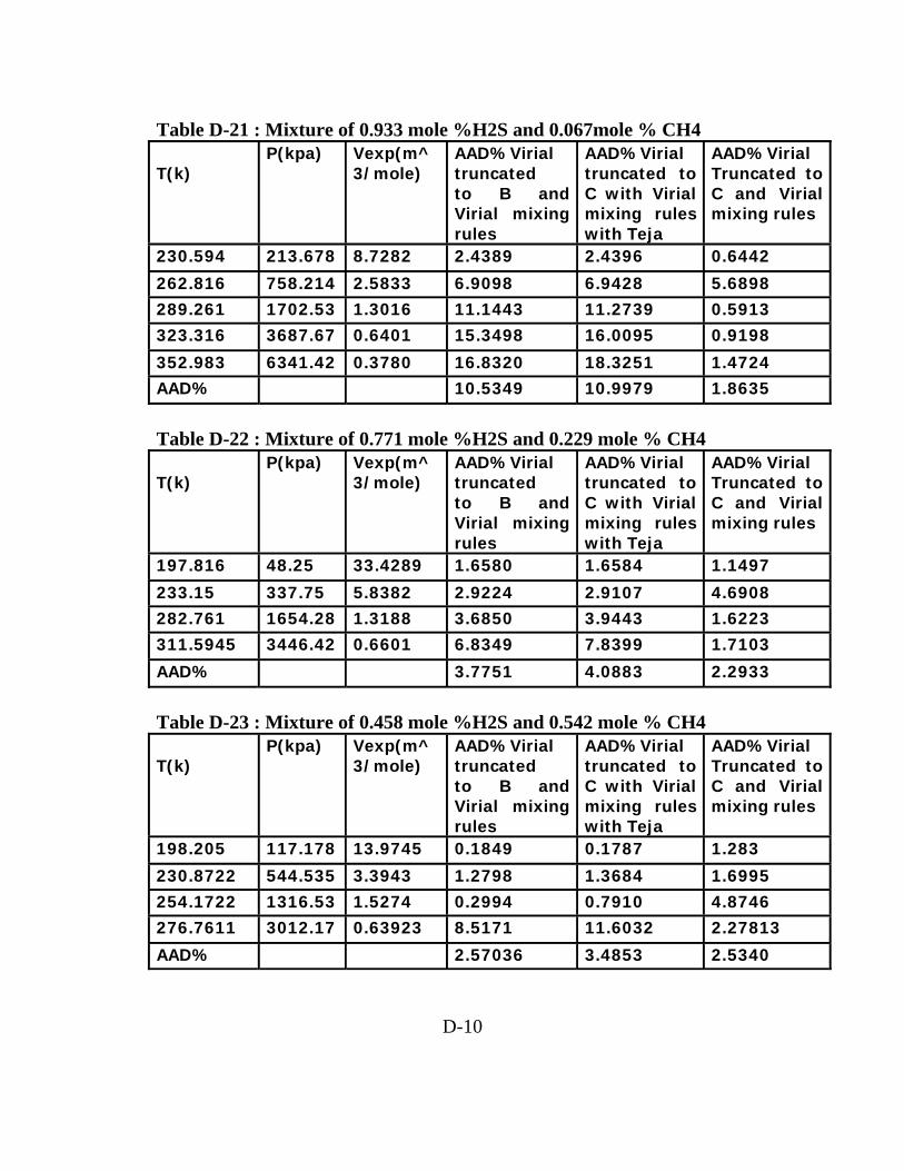
Table D-21 : Mixture of 0.933 mole %H2S and 0.067mole % CH4 T(k)

P(kpa) Vexp(m^3/mole)

AAD%Virial truncated to B and Virial mixing rules

AAD%Virial truncated to C with Virial mixing rules with Teja

AAD%Virial Truncated to C and Virial mixing rules

230.594 213.678 8.7282 2.4389 2.4396 0.6442

262.816 758.214 2.5833 6.9098 6.9428 5.6898 289.261 1702.53 1.3016 11.1443 11.2739 0.5913 323.316 3687.67 0.6401 15.3498 16.0095 0.9198

352.983 6341.42 0.3780 16.8320 18.3251 1.4724 AAD% 10.5349 10.9979 1.8635

Table D-22 : Mixture of 0.771 mole %H2S and 0.229 mole % CH4 T(k)

P(kpa) Vexp(m^3/mole)

AAD%Virial truncated to B and Virial mixing rules

AAD%Virial truncated to C with Virial mixing rules with Teja

AAD%Virial Truncated to C and Virial mixing rules

197.816 48.25 33.4289 1.6580 1.6584 1.1497

233.15 337.75 5.8382 2.9224 2.9107 4.6908 282.761 1654.28 1.3188 3.6850 3.9443 1.6223 311.5945 3446.42 0.6601 6.8349 7.8399 1.7103

AAD% 3.7751 4.0883 2.2933

Table D-23 : Mixture of 0.458 mole %H2S and 0.542 mole % CH4 T(k)

P(kpa) Vexp(m^3/mole)

AAD%Virial truncated to B and Virial mixing rules

AAD%Virial truncated to C with Virial mixing rules with Teja

AAD%Virial Truncated to C and Virial mixing rules

198.205 117.178 13.9745 0.1849 0.1787 1.283

230.8722 544.535 3.3943 1.2798 1.3684 1.6995 254.1722 1316.53 1.5274 0.2994 0.7910 4.8746 276.7611 3012.17 0.63923 8.5171 11.6032 2.27813

AAD% 2.57036 3.4853 2.5340

D-10

Table D-24 : Mixture of 0.15 mole %H2 and 0.85 mole % CH4 T(k)

P(kpa) Vexp(m^3/mole)

AAD%Virial truncated to B and Virial mixing rules

AAD%Virial truncated to C with Virial mixing rules with Teja

AAD%Virial Truncated to C and Virial mixing rules

373.15 3510.1 0.617169 4.5891 5.4500 4.2067

270 3464 0.617169 4.7373 5.6011 4.2743 260 3315.2 0.617169 5.3122 6.187 4.5767 250 3169.4 0.617131 5.8466 6.7330 4.8111

240 3021.8 0.617131 6.4879 7.3880 5.1197 230 2869.8 0.617131 7.3585 8.2755 5.6170 220 2719.9 0.617131 8.2415 9.1775 6.0822 210 2569.7 0.617093 9.2456 10.2038 6.6139 200 2418.2 0.61709 10.4244 11.4091 7.2538 190 2266.1 0.61705 11.79512 12.8116 8.0042 AAD% 7.40386 8.3236 5.6559

D-11

الخلاصة

بعض التنبؤ بالحجم المولي للبخار المشبع يمكن ان يحسب من عدد من معادلات الحالة، ال

ى الطور ا يطبق عل بعض منه ازي ،وال سائل والغ ى آلا الطورين ال من هذه المعادلات يطبق عل

ولي للبخار المشبع النقيةللمرآبات . ان دقة هذه المعادلات مختلفة . الغازي فقط يمكن ،الحجم الم

دا عن الحجم ان يحسب من عدد من المعادلات مثل معادلة لي آسلر التي تعطي انحراف عالي ج

ات ر 72(المولي المقاس عمليا ،وقد استعملت لحساب الحجم المولي لثلاث مرآب ة وغي نقطة قطبي

دل ) قطبية ة لمع سبة مئوي أ مع ن دما وج ، 62.8654 الخط دا فلا توجد دوعن ه عالي ج ان انحراف

ات ه لاستخ حاج ة للمرآب ذه المعادل دلك .الأخرى دام ه ة ري اني – معادل ة سواف هي ث ة حال معادل

ذا المشروع ولي في ه د استخدمت لحساب الانحراف للحجم الم دل أعطت ،وق ة لمع سبة مئوي ن

غ ). نقطة 299( عشرة مرآب لأربع% 15.3125 الخطأ ة بين ة الحال سو -معادل استخدمت نروبن

% .14.3476 الخطأ نسبة مئوية لمعدل وأعطت نقطة 299ت على في هذا المشروع وطبق

را ولي واخي م الم ساب الحج ستعمل لح ن ان ت ي يمك ال والت ة فيري ة الحال ال (معادل ة فيري معادل

ال المقطوعة )المقطوعة للحد الثاني و معادلة فيريال المقطوعة للحد الثالث ة فيري ،استخدام معادل

دل للحد الثاني تعطي نسبة مئو ة لمع أ ي ة (نقطة 299ل% 7.5525 الخط ر قطبي ة وغي ذا )قطبي وه

ا الحد أنالانحراف العالي نسبيا سببه سبيا بينم ة ن ذا المشروع عالي ات في ه حدود بعض المرآب

سبيا ة ن ستعمل لضغوط واطئ ار 15 زلا تتجاو (الثاني ي ال المقطوعة للحد ) . ب ة فيري ا معادل بينم

دل الثالث تعطي نتائج افضل حيث ة لمع سبة المئوي أ ان الن ه يمكن % 1.0955 هي الخط ذا لان ه

). بار50تصل الى (استخدامها لضغوط حدودها اآبر من معادلة فيريال المقطوعة للحد الثاني

ة أحسن ندرك ان معادلة فيريال المقطوعة هي أن ،يمكن بسهولة أعلاهمن المقارنة معادل

معادلة المقطوعة للحد الثالث هي إن أيضاومن الواضح يمكن استخدامها لحساب الحجم المولي ،

سن سبة لل أح اني بالن د الث ة للح ن المقطوع شروع م ذا الم ي ه ودة ف روف الموج ضغوط و (ظ ال

) .درجات الحرارة

اط يجب م أنالارتب راف للحج ل الانح ي تقل ال لك ة فيري املات لمعدل ذه المع ى ه تم عل ي

اني وباستخدام الطرق . المولي المحسوب من تلك المعادلات الإحصائية بالنسبة لمعامل فيريال الث

ى 7.5525التعديل قد حسن نسبة الانحراف من فان الارتباط قد طور وهذا باستخدام 3.5209 إل

. نقاط 210 مرآبات وبعدها طبق هذا التطوير على لأربع نقطة 89

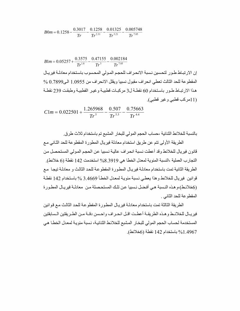
85.721.331.2005748.001325.01258.03017.01258.00TrTrTrTr

mB −−−−=

85.738.1

002184.047155.03575.005257.01TrTrTr

mB −−+=

ال إن ة فيري تخدام معادل سوب باس ولي المح م الم راف للحج سبة الانح سين ن ور لتح اط ط الارتب

ى 1.0955انحراف مقبول نسبيا ويقلل الانحراف من المقطوعة للحد الثالث تعطي % 0.7899 ال

تخدام ور باس اط ط ذا الارتب ة ل60ه ات قطب3 نقط ت مرآب ة وطبق ر القطبي ة وغي ة 239ي نقط

).قطبيطبي وغير مرآب ق11(

4.45.55

75663.0507.0265968.1022501.01TrTrTr

mC −−+=

. ،حساب الحجم المولي للبخار المشبع تم باستخدام ثلاث طرقالثنائيةبالنسبة للخلائط

اني مع الأولىالطريقة تتم عن طريق استخدام معادلة فيريال المطورة المقطوعة للحد الث

سبيا عن الحجم أعطتقانون فيريال للخلائط وقد ة ن سبة انحراف عالي ولي المستحصل من ن الم

). خلائط6( نقطة 142استخدمت % 8.3919هي خطا المئوية لمعدل النسبة التجارب العملية ،ال

ا ة تيج ال المطورة المقطوعة للحد الثالث و معادل ة فيري مع الطريقة الثانية تمت باستخدام معادل

دل وهذا يعطي فيريال للخلائط قوانين ة لمع سبة مئوي أ ن نقطة 142باستخدام %3.4669 الخط

ط6( ي )خلائ سبة ه ذه الن ضل،وه ن أف صلة م ك المستح ن تل سبيا ع ورة ن ال المط ة فيري معادل

.لمقطوعة للحد الثانيا

ال الطريقة الثالثة تمت باستخدام ة فيري وانين المقطوعة للحد المطورة معادل الثالث مع ق

ط ال للخلائ ة فيري ذه الطريق ت وه ة أعط سن دق راف واح ل انح سابقتين اق ريقتين ال ن الط م

ة المستخدمة لحساب الحجم المولي ا ،للبخار المشبع للخلائط الثنائي دل الخط ة لمع سبة مئوي هي ن

).خلائط6( نقطة 142باستخدام % 1.4967

شكر وتقدير

ى رم عل داالله المحت دآتور محمود عمر عب ى الاستاذ ال ان ال اتقدم بجزيل الشكر و الامتند . نصائه القيمة والجهد المبذول م اجل انجاز هذا المشروع سيد عمي ى ال شكر ال دم بال ا واتق آم

رم ة المحت دماه من دعم آلية الهندسة المحترم والسيد رئيس قسم الهندسة الكيمياوي ا ق ى م عل .ومساعدة

ى ابي وامي دنيا ال ذه ال واخيرا اتقدم بجزيل شكري وعظيم امتناني الى اغلى من في هشجيعهم دعمهم المتواصل وت ائلتي ل راد ع ع اف ى جمي راح والاحزان وال والى زوجي شريك الاف

.الدائم ومساعدتهم في انجاز هذا المشروع

التحقق من الارتباطات للتنبؤ بحجم البخار المشبع

للمرآبات النقية والخلائط

رسالة مقدمة إلى آلية الهندسة

و هي جزء في جامعة النهرين نيل درجة من متطلبات

ماجستير علوم في

الهندسة الكيمياوية

من قبل

ورقاء عبدالرضا آاظم الشمري ٢٠٠٣ في الهندسة الكيمياوية علوموريوسالبك

١٤٢٧ ربيع الثاني

٢٠٠٦ آيار