Investigation of Some Image and Video Coding Techniques

Investigation of Some Image andVideo Coding Techniques

Praveen Kumar Rohit

under the guidance of

Prof. Banshidhar Majhi

Department of Computer Science and Engineering

National Institute of Technology Rourkela

Rourkela – 769 008, India

Investigation of Some Imageand Video Coding Techniques

Thesis submitted in

May 2010

to the department of

Computer Science and Engineering

of


in partial fulfillment of the requirements

for the degree of

B.Tech

by

Praveen Kumar Rohit

(Roll 10606054)

Prof. Banshidhar Majhi

Department of Computer Science and Engineering


Rourkela – 769 008, India

Department of Computer Science and EngineeringNational Institute of Technology RourkelaRourkela-769 008, India. www.nitrkl.ac.in

Banshidhar MajhiProfessor

May 7, 2010

Certificate

This is to certify that the work in this Thesis Report entitled Investigation of

some Image and Video coding Techniques submitted by Praveen Kumar Rohit,

has been carried out under my supervision and guidance, in partial fulfillment of

the requirements for the degree of Bachelor of Technology in Computer Science

during session 2006-2010 in the Department of Computer Science and Engineering,

National Institute of Technology, Rourkela. To the best of my knowledge, the

matter embodied in the thesis is authentic and has not been submitted to any

other University/Institute for the award of any Degree or Diploma.

Banshidhar Majhi

Acknowledgment

No thesis is created entirely by an individual, many people have helped to create

this thesis and each of their contribution has been valuable.

The enthusiastic guidance and support of Prof. Banshidhar Majhi inspired

me to stretch beyond my limits. His profound insight has guided my thinking to

improve the final product. My solemnest gratefulness to him.

My sincere thanks to Prof. P. K. Sa and the Research Scholar Mr. Suvendu

Rupfor their continuous encouragement and invaluable advice.

Their consistent support and intellectual guidance made us energize and

innovate new ideas.

Last, but not least we would like to thank all the professors and lecturers,

and members of the Department of Computer Science and Engineering, National

Institute of Technology, Rourkela for their generous help in various ways for the

completion of this thesis.

Finally, my heartfelt thanks to my family for their unconditional love and

support. Words fail me to express my gratitude to my beloved parents, who

sacrificed their comfort for my betterment.

Praveen Kumar Rohit

Abstract

Image compression refers to the process of reducing the quantity of data used to

represent digital images, and is a combination of spatial image compression and

temporal motion compensation. Spatial image compression is done by exploiting

the spatial redundancy. Temporal motion compensation is done by exploiting the

correlation of the pixels in the nearby frame. Images require substantial storage

and transmission resources, thus image compression is advantageous to reduce

these requirements. The report covers some background of wavelet analysis, data

compression and how wavelets have been and can be used for image compression

and some of the block matching techniques for motion estimation.

In this thesis, investigations have been made to understand the actual

mechanism of compression of still images and applying the principle to the video

frames. Initially image compression is analyzed using wavelet transform and then

it is implemented. In later stages motion estimation techniques are analyzed so as

to achieve compression by exploiting the temporal redundancy. Three algorithms

for motion estimation are analyzed and compared with each other through their

results.

Contents

Certificate ii

Acknowledgement iii

Abstract iv

List of Figures vii

1 Introduction 1

1.1 Background . . . . . . . . . . . . . . . . . . . . . . . . . . . . . . . 2

1.2 Objective for Image compression . . . . . . . . . . . . . . . . . . . . 2

1.3 Types of Data Compression . . . . . . . . . . . . . . . . . . . . . . 3

1.3.1 Lossless compression . . . . . . . . . . . . . . . . . . . . . . 3

1.3.2 Lossy Compression . . . . . . . . . . . . . . . . . . . . . . . 3

1.3.3 Compression for removing Spatial Redundancy . . . . . . . . 5

1.3.4 Compression for removing Temporal Redundancy . . . . . . 5

1.4 Objective for Image Compression . . . . . . . . . . . . . . . . . . . 5

2 Related Work 6

2.1 Image Compression using Wavelet Transform . . . . . . . . . . . . . 7

2.1.1 Introduction . . . . . . . . . . . . . . . . . . . . . . . . . . . 7

2.2 Multiresolution and Wavelets . . . . . . . . . . . . . . . . . . . . . 7

2.3 The Continuous Wavelet Transform (CWT) . . . . . . . . . . . . . 7

2.4 Discrete Wavelet Transform(DWT) and subsignal encoding . . . . 8

2.5 EZW (Embedded Zerotrees of Wavelet Transforms) . . . . . . . . . 10

2.6 Set partitioning in hierarchical trees (SPIHT) . . . . . . . . . . . . 11

v

3 Fast Motion Estimation 14

3.1 Introduction . . . . . . . . . . . . . . . . . . . . . . . . . . . . . . . 15

3.2 Block Matching Algorithm . . . . . . . . . . . . . . . . . . . . . . . 15

3.2.1 Exhaustive search . . . . . . . . . . . . . . . . . . . . . . . . 17

3.2.2 Three Step Search(TSS) . . . . . . . . . . . . . . . . . . . . 18

3.2.3 Four Step Search(4SS) . . . . . . . . . . . . . . . . . . . . . 19

3.2.4 Two Dimensional Logarithmic Search(TDL) . . . . . . . . . 19

3.2.5 New Three Step Search(NTSS) . . . . . . . . . . . . . . . . 20

3.2.6 Cross Seaerch(CS) . . . . . . . . . . . . . . . . . . . . . . . 21

4 Implementation and Result 24

4.1 Image Compression Using Wavelet Transform . . . . . . . . . . . . 25

4.2 Fast Motion Estimation . . . . . . . . . . . . . . . . . . . . . . . . 28

5 Conclusion 29

Bibliography 31

vi

List of Figures

2.1 subband decomposition . . . . . . . . . . . . . . . . . . . . . . . . . 9

2.2 Down sampling . . . . . . . . . . . . . . . . . . . . . . . . . . . . . 10

3.1 Block Matching . . . . . . . . . . . . . . . . . . . . . . . . . . . . . 16

3.2 Three Step Search Procedure . . . . . . . . . . . . . . . . . . . . . 18

3.3 Four Step Search Procedure . . . . . . . . . . . . . . . . . . . . . . 19

3.4 Two Dimensional Logarithmic Search(TDL) . . . . . . . . . . . . . 20

3.5 New Three Step Search(NTSS) . . . . . . . . . . . . . . . . . . . . 21

3.6 Cross Search(CS) . . . . . . . . . . . . . . . . . . . . . . . . . . . . 22

4.1 Resultant Image.bmp . . . . . . . . . . . . . . . . . . . . . . . . . . 25

4.2 Resultant Image.jpg . . . . . . . . . . . . . . . . . . . . . . . . . . 26

4.3 Resultant Image.png . . . . . . . . . . . . . . . . . . . . . . . . . . 27

vii

Chapter 1

Introduction

1

Chapter 1 Introduction

1.1 Background

Uncompressed multimedia (graphics, audio and video) data requires considerable

storage capacity and transmission bandwidth. Despite rapid progress in

mass-storage density, processor speeds, and digital communication system

performance, demand for data storage capacity and data-transmission bandwidth

continues to outstrip the capabilities of available technologies. The recent growth

of data intensive multimedia-based web applications have not only sustained

the need for more efficient ways to encode signals and images but have made

compression of such signals central to storage and communication technology.

Image compression is minimizing the size in bytes of a graphics file without

degrading the quality of the image to an unaccceptable level. The reduction in

file size allows more images to be stored in a given amount of disk or memory

space. It also reduces the time required for images to be sent over the Internet or

downloaded from Web pages.

For still image compression, the ‘Joint Photographic Experts Group’

or JPEGstandard has been established by ISO (International Standards

Organization) and IEC (International Electro-Technical Commission). The

performance of these coders generally degrades at low bit-rates mainly because

of the underlying block-based Discrete Cosine Transform (DCT) scheme. More

recently, the wavelet transform has emerged as a cutting edge technology, within

the field of image compression. Wavelet-based coding provides substantial

improvements in picture quality at higher compression ratios.Over the past

few years, a variety of powerful and sophisticated wavelet-based schemes for

image compression have been developed and implemented. Because of the many

advantages, JPEG-2000 standard are wavelet-based compression algorithms.

1.2 Objective for Image compression

Images contain large amounts of information that requires much storage space,

large transmission bandwidths and long transmission times. Therefore it is

2


advantageous to compress the image by storing only the essential information

needed to reconstruct the image. An image can be thought of as a matrix of

pixel (or intensity) values. In order to compress the image, redundancies must be

exploited, for example, areas where there is little or no change between pixel values.

Therefore images having large areas of uniform colour will have large redundancies,

and conversely images that have frequent and large changes in colour will be less

redundant and harder to compress. [1]

1.3 Types of Data Compression

Types of data compression(according to data loss):

Lossless compression

Lossy compression

1.3.1 Lossless compression

Lossless data compression is a class of data compression algorithms that allows

the exact original data to be reconstructed from the compressed data. Lossless

compression is used when it is important that the original and the decompressed

data be identical, or when no assumption can be made on whether certain

deviation is uncritical. Lossless compression is necessary for text, where every

character is important. In other words each and every input symbol is very vital.

Typical examples are executable programs and source code.

1.3.2 Lossy Compression

A Lossy data compression method is one where compressing data and then

decompressing it retrieves data that may well be different from the original but

is close enough to be useful in some way. It allows an approximation of the

original data to be reconstructed in exchange for better compression rates. In

many applications this lack of exact reconstruction is not a major problem. For

3


example, while transmission of speech each and every value of sound sample is

not important. The thing that matters the quality of the reconstructed speech is

within tolerable limits or not.

Advantages of data compression:

More memory space is available for use

Files can be uploaded and downloaded faster

Increase in file storage options

Disadvantages of data compression:

Increase in complexity

Detrimental effect of transmission error

Slower processing for sophisticated techniques

Requirement for decompressing the previous data

Techniques to achieve video compression(according to data

redundancy)

Compression for removing Spatial Redundancy

Compression for removing Temporal Redundancy

4


1.3.3 Compression for removing Spatial Redundancy

Since the pixels in a frame of most 2-D intensity arrays are similar to nearby

neighbour pixels,information is unnecessarily replicated in the representation

of the correlated pixels. Spatial compression exploits this property of spatial

redundancy in the frames to achieve compression.This compression technique is

applied to individual frames. The data considered by the encoder is self-contained

within a single picture and bears no relationship to other frames in a sequence.

Like this sequence of frames are coded by simple video codecs.Motion JPEG is an

example of this type of codec.

1.3.4 Compression for removing Temporal Redundancy

Generally in a video sequence,pixels in a frame are similar or dependent on pixels

in the nearby frames.This property of pixels being temporally correlated is called

temporal redundancy.Temporal compression exploits this property of temporal

redundancy between the frames to achieve compression. This compression

technique is always lossy,because it is founded on the concept of calculating the

differences between successive images and describing those differences, without

having to repeat the description of any part of the image that is unchanged. [2]

1.4 Objective for Image Compression

As stated previously uncompressed data requires considerable storage capacity and

transmission bandwidth. Despite rapid progress in mass-storage density, processor

speeds, and digital communication system performance, demand for data storage

capacity and data-transmission bandwidth continues to outstrip the capabilities

of available technologies.Image compression is minimizing the size in bytes of a

graphics file without degrading the quality of the image to an unaccceptable level.

The reduction in file size allows more images to be stored in a given amount of

disk or memory space. It also reduces the time required for images to be sent over

the Internet or downloaded from Web pages.

5

Chapter 2

Related Work

6

Chapter 2 Related Work

2.1 Image Compression using Wavelet

Transform

2.1.1 Introduction

Wavelets are functions defined over a finite interval and having an average value

of zero. The basic idea of the wavelet transform is to represent any arbitrary

function (t) as a superposition of a set of such wavelets or basis functions. These

basis functions or baby wavelets are obtained from a single prototype wavelet

called the mother wavelet, by dilations or contractions (scaling) and translations

(shifts). The Discrete Wavelet Transform of a finite length signal x(n) having N

components, for example, is expressed by an N x N matrix.Wavelet compression

is a form of data compression well suited for image compression. Using a

wavelet transform, the wavelet compression methods are adequate for representing

transients, such as percussion sounds in audio, or high-frequency components in

two-dimensional images, for example an image of stars on a night sky. [2]

2.2 Multiresolution and Wavelets

The power of Wavelets comes from the use of multiresolution. Rather than

examining entire signals through the same window, different parts of the wave

are viewed through different size windows (or resolutions). High frequency parts

of the signal use a small window to give good time resolution, low frequency parts

use a big window to get good frequency information

2.3 The Continuous Wavelet Transform (CWT)

The continuous wavelet transform is the sum over all time of scaled and

shifted versions of the mother wavelet Ã. Calculating the Continuous Wavelet

Transform(CWT) results in many coefficients C, which are functions of scale and

7


translation.

C(s, t) =

∫f(t)Ã(s, ¿, t)d(t) (2.1)

where

• The translation, ¿ , is proportional to time information

• the scale, s,is proportional to inverse of frequency information

To find the constituent wavelets of the signal, the coefficients should be multiplied

by the relevant version of the mother wavelet.

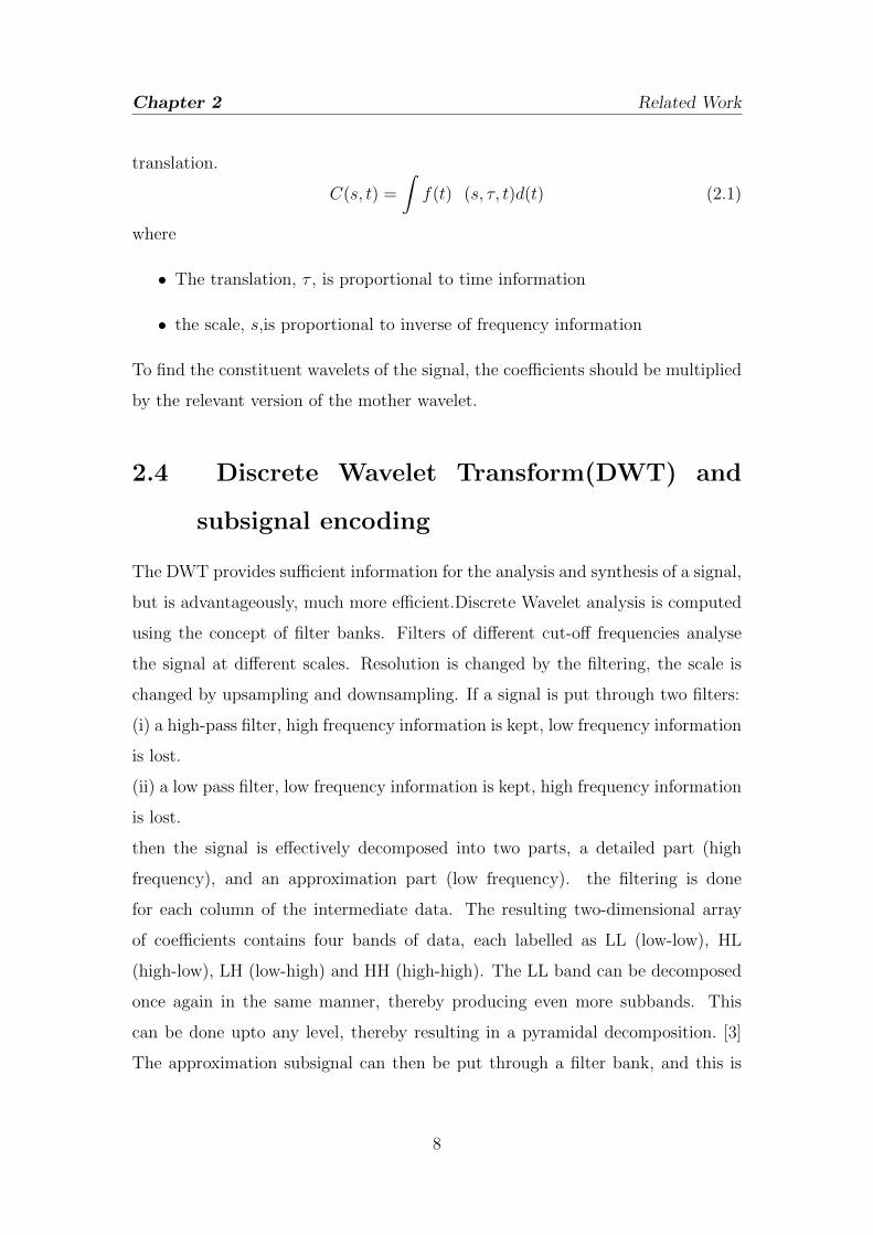
2.4 Discrete Wavelet Transform(DWT) and

subsignal encoding

The DWT provides sufficient information for the analysis and synthesis of a signal,

but is advantageously, much more efficient.Discrete Wavelet analysis is computed

using the concept of filter banks. Filters of different cut-off frequencies analyse

the signal at different scales. Resolution is changed by the filtering, the scale is

changed by upsampling and downsampling. If a signal is put through two filters:

(i) a high-pass filter, high frequency information is kept, low frequency information

is lost.

(ii) a low pass filter, low frequency information is kept, high frequency information

is lost.

then the signal is effectively decomposed into two parts, a detailed part (high

frequency), and an approximation part (low frequency). the filtering is done

for each column of the intermediate data. The resulting two-dimensional array

of coefficients contains four bands of data, each labelled as LL (low-low), HL

(high-low), LH (low-high) and HH (high-high). The LL band can be decomposed

once again in the same manner, thereby producing even more subbands. This

can be done upto any level, thereby resulting in a pyramidal decomposition. [3]

The approximation subsignal can then be put through a filter bank, and this is

8


Figure 2.1: subband decomposition

9


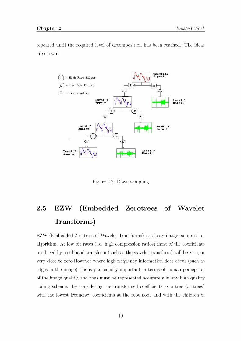
repeated until the required level of decomposition has been reached. The ideas

are shown :

Figure 2.2: Down sampling

2.5 EZW (Embedded Zerotrees of Wavelet

Transforms)

EZW (Embedded Zerotrees of Wavelet Transforms) is a lossy image compression

algorithm. At low bit rates (i.e. high compression ratios) most of the coefficients

produced by a subband transform (such as the wavelet transform) will be zero, or

very close to zero.However where high frequency information does occur (such as

edges in the image) this is particularly important in terms of human perception

of the image quality, and thus must be represented accurately in any high quality

coding scheme. By considering the transformed coefficients as a tree (or trees)

with the lowest frequency coefficients at the root node and with the children of

10


each tree node being the spatially related coefficients in the next higher frequency

subband, there is a high probability that one or more subtrees will consist entirely

of coefficients which are zero or nearly zero, such subtrees are called zerotrees.

EZW uses four symbols to represent (a) a zerotree root, (b) an isolated zero

(a coefficient which is insignificant, but which has significant descendants), (c)

a significant positive coefficient and (d) a significant negative coefficient. The

symbols may be thus represented by two binary bits. The compression algorithm

consists of a number of iterations through a dominant pass and a subordinate

pass, the threshold is updated (reduced by a factor of two) after each iteration.

2.6 Set partitioning in hierarchical trees

(SPIHT)

The SPHIT uses a partitioning of tree (which in SPHIT are called spatial

orientation trees) in a mannes that tends to keep insignificant coefficients together

in larger subsets.The trees are further divide into four types of sets:

∗ O(i, j)- set of co-ordinates of offspring of wavelet co-efficient at location(i,j).

∗ D(i, j)- set of all descendants of coefficients at location(i,j).

∗ ℋ- set of all root nodes.

∗ ℒ(i, j)- set of coordinates of all descendants of coefficient at location(i,j), except

for immediate offspring of coefficient at location (i,j)

ℒ(i, j)= D(i, j)-O(i, j)

The SPIHT algorithm uses three list:

∗List of insignificant pixels(LIP).∗List of significant pixels(LSP).∗List of insignificant sets(LIS).

11


The SPIHT algorithm are as follows:

Step(i):Initialization

n = ⌊log2cmax⌋Set LIP = All elements in H

Set LSP = Empty

Set LIS = Ds of Roots

Step(ii):Significance Map Encoding

Process LIP

for each coeff (i,j) in LIP

Then, Output Sn(i,j)

If Sn(i,j)=1

Output sign of coeff(i,j): 0/1 = -/+

Move (i,j) to the LSP

End if

End loop over LIP

Process LIS

for each set (i,j) in LIS

if type D

Send Sn(D(i,j))

If Sn(D(i,j))=1

for each (k,l)² O(i,j)

output Sn(k,l)

if Sn(k,l)=1, then add (k,l) to the LSP and output sign of coeff: 0/1 = -/+

if Sn(k,l)=0, then add (k,l) to the end of the LIP

end for

end if

else (type L )

Send Sn(L(i,j))

If Sn(L(i,j))=1

add each (k,l) ² O(i,j) to the end of the LIS as an entry of type D

remove (i,j) from the LIS

12


end if on type

End loop over LIS

Step(iii):Refinement Pass

Process LSP

for each element (i,j) in LSP except those just added above

Output the nth most significant bit of coeff

End loop over LSP

Update

Decrement n by 1

Go to Significance Map Encoding Step

The partitioning decisions are binary deciasions that are transmitted to decoder,

providing a significance map encoding that is more efficient than EZW. [4]

13

Chapter 3

Fast Motion Estimation

14

Chapter 3 Fast Motion Estimation

3.1 Introduction

Motion estimation is the process of determining motion vectors that describe the

transformation from one 2D image to another; usually from adjacent frames in a

video sequence. It is an ill-posed problem as the motion is in three dimensions but

the images are a projection of the 3D scene onto a 2D plane. The motion vectors

may relate to the whole image (global motion estimation) or specific parts, such

as rectangular blocks, arbitrary shaped patches or even per pixel. The motion

vectors may be represented by a translational model or many other models that can

approximate the motion of a real video camera, such as rotation and translation

in all three dimensions and zoom. The methods for finding motion vectors can

be categorised into pixel based methods (”direct”) and feature based methods

(”indirect”). Motion estimation is an indispensable part of video compression

and video processing. It helps to bring out information about motion of certain

objects or features from the video sequence. The motion is typically represented

using a motion vector (x,y). The motion vector gives the displacement of a

pixel or a pixel block (called macroblock) from the current pixel or macroblock

location due to motion. Motion vector which contains motion information helps

to find out best matching block using block matching techniques to generate and

predict temporally interpolated frames. It is also used in applications such motion

compensated de-interlacing, video stabilization, motion tracking etc. There are

several kinds of motion estimation techniques available. Some work on a pixel

level and find motion vector for each pixel. However the most well known and

widely used technique is block matching algorithm (BMA).

3.2 Block Matching Algorithm

Block matching finds the motion vector not for a single pixel but for a group

of pixels called a macroblock. Some common macroblock sizes are 8X8 and

16X16 pixels. The are square shaped macroblocks. Using macroblocks instead

of individual pixels saves on computations greatly and is also more intelligent

15


and intuitive as objects have features in clusters rather than manifesting in

single pixels. Block matching is illustrated in the figure. The frame under

Figure 3.1: Block Matching

consideration is divided in to macroblocks and motion estimation is performed

on each macroblock. Motion estimation is done by identifying a pixel block

from the reference frame that best matches the current block, whose motion is

being estimated. The reference macroblock is created by displacement from the

current blocks location in the reference frame. This displacement is denoted by

the motion vector (MV). MV consists of is a pair (x, y) of horizontal and vertical

displacement values. Two popular techniques for finding a block match among so

many techniques available are Sum of square error(SSE)

N∑x=1

N∑y=1

(C(x, y)−R(x, y))2 (3.1)

And the other one is , Sum of absolute differences (SAD)

N∑x=1

N∑y=1

∣C(x, y)−R(x, y)∣ (3.2)

SSE is a better block matching technique as it gives better results in case

a match does exist at the subjective human perception level , however is

computationally more burdensome than the SAD technique which also gives fairly

16


good estimates of a match if found. Hence there are other parameters that might

also be checked to ensure better results like cross correlation, maximum matching

pixel count etc. The reference pixel blocks are created only from a region called

the search window or search area. Search window limits the number of blocks to

be evaluated. The size of this window invariably depends on the amount of motion

present and the computational challenge that can be dealt with properly. Larger

search window demands more computation as it should be. Typically the search

region is kept wider (i.e. width is more than height) since many video sequences

often exhibit panning motion. The horizontal and vertical search range, Sx and

Sy, define the search area (+/-Sx and +/- Sy) as illustrated in figure.

There are various cost functions, of which the most popular and less

computationally expensive is Mean Absolute Difference (MAD) .

MAD =1

N2

N∑x=1

N∑y=1

∣C(x, y)−R(x, y)∣ (3.3)

Another cost function is Mean Squared Error (MSE) .

MSE =1

N2

N∑x=1

N∑y=1

(C(x, y)−R(x, y))2 (3.4)

3.2.1 Exhaustive search

Exhaustive search generates the best block matching motion vectors because it

searches every block in the search window. However due to astronomically high

number of computations required, this technique can result in prohibitive cost of

computation. The number of candidates to evaluate are (2Sx+1)*(2Sy+1). There

are several other fast block matching algorithms available that reduce number of

computations required significantly at the cost of slightly reducing performance

because these techniques find the local minima and not the global one as in case

of full or extensive search.

17


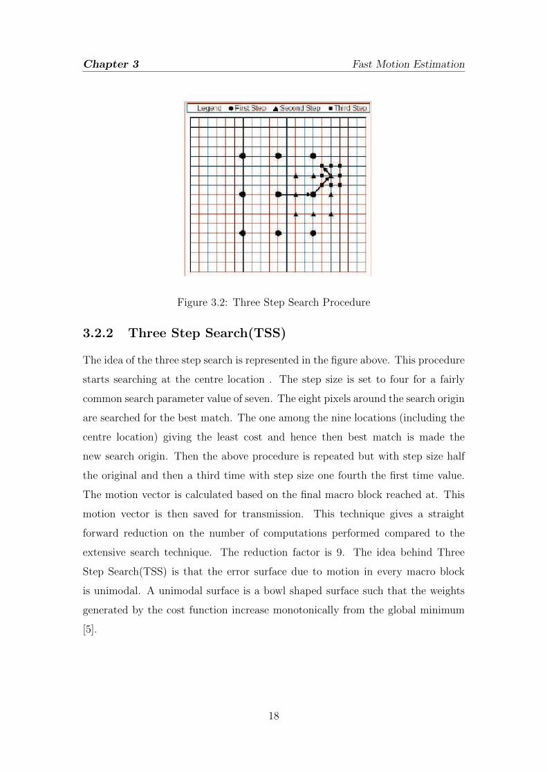
Figure 3.2: Three Step Search Procedure

3.2.2 Three Step Search(TSS)

The idea of the three step search is represented in the figure above. This procedure

starts searching at the centre location . The step size is set to four for a fairly

common search parameter value of seven. The eight pixels around the search origin

are searched for the best match. The one among the nine locations (including the

centre location) giving the least cost and hence then best match is made the

new search origin. Then the above procedure is repeated but with step size half

the original and then a third time with step size one fourth the first time value.

The motion vector is calculated based on the final macro block reached at. This

motion vector is then saved for transmission. This technique gives a straight

forward reduction on the number of computations performed compared to the

extensive search technique. The reduction factor is 9. The idea behind Three

Step Search(TSS) is that the error surface due to motion in every macro block

is unimodal. A unimodal surface is a bowl shaped surface such that the weights

generated by the cost function increase monotonically from the global minimum

[5].

18


Figure 3.3: Four Step Search Procedure

3.2.3 Four Step Search(4SS)

Four step searching is also a centre based searching technique and has a halfway

stopping provision [1]. Irrespective of the value of the parameter p, Four Step

Search(4SS) has a search parameter value of S=2. Thus it looks for a match among

the 9 windows in a 5X5 neighborhood. If the least weight is found at the center

of search window the search jumps to fourth step. If the least weight is at one of

the eight locations except the center, then we make it the search origin and move

to the second step. Even now the search window is maintained 5X5 pixels wide.

Depending on the last best match block we have to check either 3 or 5 locations

as depicted in the figure. If the best match is at the centre of the window we go

to 4th step. If not then we go into the third step of the procedure. The third step

is a repetition of the second step. In the 4th step the search window is made of

size 3X3, i.e. S=1. The location with best match is set as the final location and

the motion vector is calculated according to that point. [6].

3.2.4 Two Dimensional Logarithmic Search(TDL)

Two Dimensional Logarithmic search is another algorithm, which tests limited

candidates. It is similar to the three-step search. During the first iteration, a

19


Figure 3.4: Two Dimensional Logarithmic Search(TDL)

total of five candidates are tested. The candidates are centred around the current

block location in a diamond shape. The step size for first iteration is set equal

to half the search range. For the second iteration, the centre of the diamond is

shifted to the best matching candidate. The step size is reduced by half only if

the best candidate happens to be the centre of the diamond. If the best candidate

is not the diamond centre, same step size is used even for second iteration. In this

case, some of the diamond candidates are already evaluated during first iteration.

Hence, there is no need for block matching calculation for these candidates during

the second iteration. The results from the first iteration can be used for these

candidates. The process continues till the step size becomes equal to one pixel.

For this iteration all eight surrounding candidates are evaluated.

3.2.5 New Three Step Search(NTSS)

New Three Step Search(NTSS) improves on Three Step Search(TSS) results by

providing a center biased searching scheme and having provisions for half way

stop to reduce computational cost. The Three Step Search(TSS) uses a uniformly

allocated checking pattern for motion detection and is prone to missing small

motions. In the first step 16 points are checked in addition to the search origin for

20


Figure 3.5: New Three Step Search(NTSS)

lowest weight using a cost function. Of these additional search locations, 8 are a

distance of S = 4 away (similar to TSS) and the other 8 are at S = 1 away from

the search origin. If the lowest cost is at the origin then the search is stopped

right here and the motion vector is set . If the lowest weight is at any one of the 8

locations at S = 1, then we change the origin of the search to that point and check

for weights adjacent to it. The location that gives the lowest weight is the closest

match and motion vector is set to that location. On the other hand if the lowest

weight after the first step was one of the 8 locations at S = 4, then we follow the

normal Three Step Search(TSS) procedure.

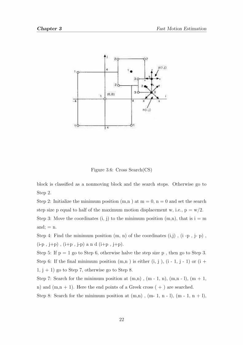
3.2.6 Cross Seaerch(CS)

In the cross search algorithm presented here, the basic idea is still a logarithmic

step search. The reference point for a block is taken to be the pel(i, j) at its upper

left hand comer. The block in the previous frame which corresponds to a block in

the current frame is referred to as the block at (0,0). The cross search algorithm

can then be described as follows.

Step 1: The current block and the block at (0,0), are compared and if the value

of the distortion function is less than a predefined threshold T then the current

21


Figure 3.6: Cross Search(CS)

block is classified as a nonmoving block and the search stops. Otherwise go to

Step 2.

Step 2: Initialize the minimum position (m,n ) at m = 0, n = 0 and set the search

step size p equal to half of the maximum motion displacement w, i.e., p = w/2.

Step 3: Move the coordinates (i, j) to the minimum position (m,n), that is i = m

and; = n.

Step 4: Find the minimum position (m, n) of the coordinates (i,j) , (i -p , j- p) ,

(i-p , j+p) , (i+p , j-p) a n d (i+p , j+p).

Step 5: If p = 1 go to Step 6, otherwise halve the step size p , then go to Step 3.

Step 6: If the final minimum position (m,n ) is either (i, j ), (i - 1, j - 1) or (i +

1, j + 1) go to Step 7, otherwise go to Step 8.

Step 7: Search for the minimum position at (m,n) , (m - 1, n), (m,n - l), (m + 1,

n) and (m,n + 1). Here the end points of a Greek cross ( + ) are searched.

Step 8: Search for the minimum position at (m,n) , (m- 1, n - l), (m - 1, n + l),

22


(m + 1, n - 1) and (rn + 1, n + 1). In this case the end points of a St. Andrews

cross (X) are searched. [7]

23

Chapter 4

Implementation and Result

24

Chapter 4 Implementation and Result

4.1 Image Compression Using Wavelet

Transform

Using bmp image PSNR:39.85 dB

Figure 4.1: Resultant Image.bmp

Using jpg image PSNR: 33.09 dB

Using png image PSNR: 27.34 dB

25


Figure 4.2: Resultant Image.jpg

26


Figure 4.3: Resultant Image.png

27


4.2 Fast Motion Estimation

algorithms Computation PSNR

Time(in sec) (dB)

Exhaustive Search 211.5 11

Three Step Search 24.1 10.7

(TSS)

Four Step Search 18.9 10.4

(FSS)

Two Dimensional Logarithmic Search 14.7 10.5

(TDL)

New Three Step Search 17.6 10.6

(NTSS)

Cross Search 14.5 10.8

(CS)

28

Chapter 5

Conclusion

29

Conclusion

Initially we have examined the actual mechanism of compressing images

by implementing wavelet transformation using SPIHT.Wavelet analysis is very

powerful and extremely useful for compressing data such as images. Its

power comes from its multiresolution.The image itself has a dramatic effect on

compression. This is because it is the images pixel values that determine the

size of the coefficients, and hence how much energy is contained within each

subsignal. Furthermore, it is the changes between pixel values that determine

the percentage of energy contained within the detail subsignals, and hence the

percentage of energy vulnerable to thresholding. Therefore, different images will

have different compressibilities.The past two decades have seen the growth of wide

acceptance of multimedia. Video compression plays an important role in archival

of entertainment based video (CD/DVD)as well as real-time reconnaissance /

video conferencing applications. While ISO MPEG sets the standard for the

former types of application, ITU sets the standards for latter low bit rate

applications. In the entire motion based video compression process motion

estimation is the most computationally expensive and time-consuming process.The

research in the past decade has focused on reducing both of these side effects of

motion estimation. Block matching techniques are the most popular and efficient

of the various motion estimation techniques.Here we have first described the

motion compensation based video compression in brief.Then we have illustrated

and simulated six of the most popular block matching algorithms, with their

comparative study at the end.

30

Bibliography

[1] Aroh Barjatya. Block matching algorithms for motion estimation. DIP 6620 Spring, 2004.

[2] Patnaik and Venugopal. Information Processing. I.K.International, 2008.

[3] Tham Jo Yew. Data processing image compression using wavelet transform. IEEE Region

10 student Paper, 1995.

[4] Khalid Sayood. Introduction to Data Compression. Academic Press, 2005.

[5] Jose. A. Garcia. Progresssive Image Transmission. International Society for Optical

Engineering, 2004.

[6] Lai-Man Po and Wing-Chung Ma. A novel four-step search algorithm for fast block motion

estimation. IEEE Trans. Circuits And Systems For Video Technology, 6(3):313 – 317, June

1996.

[7] M. Ghanbari. Cross search algorithm for motion estimation. IEEE, 38.

[8] Nikola Sprljan. Modified spiht algorithm for wavelet packet image coding. WP-SPIHT,

August 2005.

31

Investigation of Some Image and Video Coding Techniques

Documents

Transcript of Investigation of Some Image and Video Coding Techniques