University of New OrleansScholarWorks@UNO

Senior Honors Theses Undergraduate Showcase

5-1-2013

Investigation of Perforated Ducted Propellers to usewith a UAVKrishna Regmi

Follow this and additional works at: http://scholarworks.uno.edu/honors_theses

This Honors Thesis-Unrestricted is brought to you for free and open access by the Undergraduate Showcase at ScholarWorks@UNO. It has beenaccepted for inclusion in Senior Honors Theses by an authorized administrator of ScholarWorks@UNO. For more information, please contactscholarworks@uno.edu.

Recommended CitationRegmi, Krishna, "Investigation of Perforated Ducted Propellers to use with a UAV" (2013). Senior Honors Theses. Paper 45.

Investigation of Perforated Ducted Propellers to use with a UAV

An Honors Thesis

Presented to

the Department of Mechanical Engineering

of the University of New Orleans

In Partial Fulfillment

Of the Requirements for the Degree of

Bachelor of Science, with University Honors

And Honors in Mechanical Engineering

by

Krishna Regmi

May 2013

ii

Acknowledgement

I would like to thank my advisor, Professor Ting Wang, for his continuous support

throughout this year. Also thanks to Professor Martin Guillot for reading the thesis and

providing me with valuable feedback. I would like to thank the Honors Department for creating

this opportunity to perform independent research. It was one of the most valuable experiences

in my undergraduate career. This acknowledgement wouldn’t be complete if I didn’t thank

graduate students of Dr. Ting Wang, especially Scott Richard for all his editorial support and

advice, Xijia Lu for help with ICEM and Fluent, Henry Long for support with computer setup, and

Rada Ragab for his excellent feedback during the midterm and end of semester presentations.

iii

CONTENTS

CONTENTS ....................................................................................................................................... iii

ABSTRACT ...................................................................................................................................... viii

Chapter 1 : INTRODUCTION ............................................................................................................. 1

History of small UAVs ................................................................................................................... 2

Classification of UAVs .................................................................................................................. 3

Fixed Wing UAVs ...................................................................................................................... 4

Rotorcraft UAVs ....................................................................................................................... 8

Flapping Wing UAVs ............................................................................................................... 12

Unconventional UAV: ............................................................................................................. 14

Ducted fan .................................................................................................................................. 15

Motivation ................................................................................................................................. 18

Objectives .................................................................................................................................. 19

Approach .................................................................................................................................... 19

Chapter 2 : SOFTWARE TRAINING ................................................................................................. 20

Case 1: Laminar Channel Flow ................................................................................................... 20

Case 2: Laminar Pipe Flow with a constant heat flux at the surface ......................................... 23

Chapter 3 : THEORY ........................................................................................................................ 26

Formulation of Momentum Equation:....................................................................................... 26

Modified Thrust Coefficient ....................................................................................................... 31

Efficiency of Duct ....................................................................................................................... 31

Navier-Stokes Equations ............................................................................................................ 32

Chapter 4 : MODELING AND SIMULATION OF AIRFLOW ............................................................... 34

3-D propeller to 2-D Disc ........................................................................................................... 34

Infinite Domain to Finite Domain .............................................................................................. 35

Sensitivity of the size of control volume: ................................................................................... 37

Wall Functions ........................................................................................................................... 39

Pressure inlet/outlet Boundary Conditions: .............................................................................. 39

Choosing Pressure Difference .................................................................................................... 41

Choosing Overall Dimensions .................................................................................................... 42

Perforations ............................................................................................................................... 43

Verification of Symmetry: 2-D Modeling ................................................................................... 46

Axisymmetrical Modeling .......................................................................................................... 48

Grid Independent Study ............................................................................................................. 48

iv

Chapter 5 : RESULTS, DISCUSSIONS AND CONCLUSIONS .............................................................. 50

Case 1: 2-D Duct with no Perforation ........................................................................................ 50

2-D Duct with 4 Perforations ..................................................................................................... 53

2-D Duct with 6 Pores: ............................................................................................................... 57

8-Perforations ............................................................................................................................ 59

Results ........................................................................................................................................ 60

Conclusions: ............................................................................................................................... 69

BIBLIOGRAPHY ............................................................................................................................... 71

Chapter 6 : APPENDICES ................................................................................................................ 74

Appendix I: Different Cases ........................................................................................................ 74

Part 1: Laminar Channel Flow .................................................................................................... 78

Part 2.1: Steady, Laminar Flow in Circular Tubes and no Heat source. ..................................... 93

Nusselt’s Number ................................................................................................................. 105

Part 3: Turbulent Pipe Flow with Constant Temperature on the walls ................................... 110

v

List of Figures

Figure 1-1: Incredible HLQ Quad rotor (Nick, 2013) ..................................................................................... 1 Figure 1-2 PARS Aerial Rescue Bot (Solon, 2013) ......................................................................................... 2 Figure 1-3 Lockheed RX-170 Sentinel (The Muslim Observer, 2010) ........................................................... 5 Figure 1-4 NASA Pathfinder (Galante, 2001) ................................................................................................ 6 Figure 1-5 Theory of Fixed Winged UAV (MIT, 1997) ................................................................................... 6 Figure 1-6 Full Sized helicopter UAV called Hummingbird (Trimble, 2009) ................................................. 9 Figure 1-7 Miniature Quadcopter (Joblin, 2010) .......................................................................................... 9 Figure 1-8 Actuator Disc Theory (Seddon and Newman, 2011) ................................................................. 10 Figure 1-9 Festo Smart-Bird (robot bird, 2011) .......................................................................................... 12 Figure 1-10 Robot Bird (Airforce, 2012) ...................................................................................................... 13 Figure 1-11 UAV that uses helium and Inversion technology to fly (Forman, 2012) .................................. 14 Figure 1-12 Examples of un-ducted and ducted propellers, and a perforated duct ................................. 16 Figure 1-13: Thrust coefficient vs. Rotor RPM from an experiment done by NASA (Martin, 2004) .......... 17 Figure 2-1 Problem Statement for Laminar channel flow .......................................................................... 20 Figure 2-2 x-velocity vs. y-coordinate for laminar channel flow................................................................. 21 Figure 2-3 skin Friction coefficient for laminar channel flow ..................................................................... 22 Figure 2-4 Problem Statement for Laminar Pipe flow with a constant heat flux ....................................... 23 Figure 2-5 Ideal velocity vs. velocity profile obtained from fluent ............................................................. 24 Figure 2-6 skin friction coefficient vs x-coordinate ..................................................................................... 24 Figure 2-7 Development of Dimensionless Temperature profile ............................................................... 25 Figure 2-8 Variation of Nusselt's number with x-coordinate ...................................................................... 25 Figure 3-1: Conservation of momentum ..................................................................................................... 28 Figure 3-2 Forces in x-direction in an infinitesimally small, moving fluid element (Anderson CFD) .......... 32 Figure 4-1 Actuator Disc Theory (Scott, 2011) ............................................................................................ 35 Figure 4-2 Case 1 - Pressure boundary conditions ..................................................................................... 40 Figure 4-3 Case 2 - Pressure boundary conditions ..................................................................................... 40 Figure 4-4 Case 3 - Pressure boundary conditions ..................................................................................... 41 Figure 4-5: 3-D Translation of an axis-symmetrical plane with 4 Pores ..................................................... 44 Figure 4-6: 2-D Duct with four Pores .......................................................................................................... 45 Figure 4-7: Contours of Static Pressure in a 2-D model .............................................................................. 47 Figure 4-8: Contours of velocity magnitude in a 2-D model ....................................................................... 47 Figure 4-9: Axissymmetrical modeling ........................................................................................................ 48 Figure 5-1 Case 1: Duct with no perforations - velocity vectors overlayed on pressure contour .............. 51 Figure 5-2 Recirculation near tip gap .......................................................................................................... 52 Figure 5-3 Contours of Static pressure - case 2 .......................................................................................... 53 Figure 5-4 velocity vectors - case 1 ............................................................................................................. 54 Figure 5-5 velocity vectors superimposed on pressure contour - case 1 ................................................... 55 Figure 5-6 Closer look at the velocity vectors superimposed on pressure contour - case 2 ...................... 56 Figure 5-7 Case 3 - velocity vectors on pressure contour ........................................................................... 57 Figure 5-8 case 3: closer look inside the duct ............................................................................................. 58 Figure 5-9 case 4 Duct Area ........................................................................................................................ 59 Figure 5-10 Case 4 - closer look inside the duct ......................................................................................... 60 Figure 5-11 variation of net Thrust with % of open area in the duct for cases with 6000 Pa after duct weight is subtracted from the thrust .......................................................................................................... 64 Figure 5-12 variation of net Thrust with % of Open Area for cases with 3000 Pa after duct weight is subtracted from the thrust ......................................................................................................................... 65

vi

Figure 5-13 Variation of net Thrust with % of Open Area for cases with 60 Pa after duct weight is subtracted from the thrust ......................................................................................................................... 66 Figure 5-14: Thrust Coefficient vs Open Area % ......................................................................................... 67 Figure 5-15: Different types of Duct Shape (Wright Jr and Piolene 2002) ................................................. 68 Figure 6-1 Duct with no Pores ..................................................................................................................... 75 Figure 6-2: Duct with four 0.1" Pores ......................................................................................................... 75 Figure 6-3 Duct with six 0.1" Diameter Pores ............................................................................................. 75 Figure 6-4 Eight 0.1" Diameter Pores.......................................................................................................... 75 Figure 6-5: Duct with four 0.3" Pores ......................................................................................................... 76 Figure 6-6: Duct with four 0.3" Pores ......................................................................................................... 76 Figure 6-7 Duct with six 0.3" Pores ............................................................................................................. 76 Figure 6-8 Duct with Eight 0.3" Diameter Pores ......................................................................................... 76 Figure 6-9 Duct with four 0.5" Pores .......................................................................................................... 77 Figure 6-10 Duct with six 0.5" Pores ........................................................................................................... 77 Figure 6-11: Duct with eight 0.5" Diameter Pores ...................................................................................... 77 Figure 6-12 Propeller with no duct ............................................................................................................. 77 Figure 6-13: Channel Flow with Boundary Conditions at T=20oC ............................................................... 78 Figure 6-14: Channel geometry to calculate the velocity profile................................................................ 80 Figure 6-15: Channel Flow with Boundary Conditions ............................................................................... 83 Figure 6-16 : Approximate shape of converging Boundary Layers. ............................................................ 84 Figure 6-17 :The velocity Profile develops into parabolic velocity profile. ................................................. 85 Figure 6-18: Comparison of Ideal velocity profile vs. the velocity profile from Fluent .............................. 86 Figure 6-19 : Skin friction-coefficient .......................................................................................................... 86 Figure 6-20 : Channel Flow with Boundary Conditions ............................................................................... 87 Figure 6-21 : Development of flow. ............................................................................................................ 87 Figure 6-22 : Velocity profiles at different locations for a channel flow .................................................... 88 Figure 6-23 : Comparison of theoretical velocity profile with the one from Fluent ................................... 89 Figure 6-24 : Skin Friction Coefficient ......................................................................................................... 89 Figure 6-25 : A close look at the skin friction coefficient. ........................................................................... 90 Figure 6-26 : Comparison with Ideal case for velocity profile .................................................................... 91 Figure 6-27 : Skin Friction Coefficient of f = 0.057 was found. ................................................................... 92 Figure 6-28 : Channel Flow with Boundary Conditions ............................................................................... 93 Figure 6-29 : Solution with only 500 elements ........................................................................................... 97 Figure 6-30 : Results from refined mesh ..................................................................................................... 98 Figure 6-31 : Velocity Profile at inlet, exit and at x=2m ............................................................................ 100 Figure 6-32 : Comparison of velocity Profile at x=2m with the Ideal velocity profile............................... 100 Figure 6-33 : Channel Flow with Boundary Conditions ............................................................................. 101 Figure 6-34 : Pipe Flow meshing ............................................................................................................... 102 Figure 6-35 : Comparison of Ideal vs. Fluent’s velocity Profile ................................................................. 103 Figure 6-36 : Increasing Temperature ....................................................................................................... 104 Figure 6-37 : Temperature Profiles ........................................................................................................... 105 Figure 6-38 : Skin friction coefficient with Axial Coordinate .................................................................... 106 Figure 6-39 : Channel Flow with Boundary Conditions ............................................................................. 107 Figure 6-40 : Development of velocity profile .......................................................................................... 107 Figure 6-41 : Comparison of ideal vs. Fluent’s velocity profile. ................................................................ 108 Figure 6-42 : Skin Friction Coefficient of 0.0392 ....................................................................................... 108 Figure 6-43 : Thermal Profile Developing ................................................................................................. 109 Figure 6-44 : Developing profile for Dimensionless Temperature ............................................................ 109

vii

Figure 6-45 : Variation of surface Nusselt’s number with the distance from the entrance. .................... 110 Figure 6-46 : Pipe Flow with Boundary Conditions ................................................................................... 111 Figure 6-47 : Comparison of velocity profile in laminar and turbulent flow. ........................................... 114 Figure 6-48 : Velocity Profiles of a turbulent Flow ................................................................................... 116 Figure 6-49: variation of Skin Friction Coefficient in turbulent flow ........................................................ 116

viii

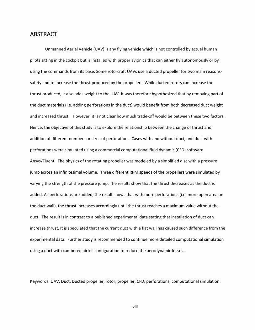
ABSTRACT

Unmanned Aerial Vehicle (UAV) is any flying vehicle which is not controlled by actual human

pilots sitting in the cockpit but is installed with proper avionics that can either fly autonomously or by

using the commands from its base. Some rotorcraft UAVs use a ducted propeller for two main reasons-

safety and to increase the thrust produced by the propellers. While ducted rotors can increase the

thrust produced, it also adds weight to the UAV. It was therefore hypothesized that by removing part of

the duct materials (i.e. adding perforations in the duct) would benefit from both decreased duct weight

and increased thrust. However, it is not clear how much trade-off would be between these two factors.

Hence, the objective of this study is to explore the relationship between the change of thrust and

addition of different numbers or sizes of perforations. Cases with and without duct, and duct with

perforations were simulated using a commercial computational fluid dynamic (CFD) software

Ansys/Fluent. The physics of the rotating propeller was modeled by a simplified disc with a pressure

jump across an infinitesimal volume. Three different RPM speeds of the propellers were simulated by

varying the strength of the pressure jump. The results show that the thrust decreases as the duct is

added. As perforations are added, the result shows that with more perforations (i.e. more open area on

the duct wall), the thrust increases accordingly until the thrust reaches a maximum value without the

duct. The result is in contrast to a published experimental data stating that installation of duct can

increase thrust. It is speculated that the current duct with a flat wall has caused such difference from the

experimental data. Further study is recommended to continue more detailed computational simulation

using a duct with cambered airfoil configuration to reduce the aerodynamic losses.

Keywords: UAV, Duct, Ducted propeller, rotor, propeller, CFD, perforations, computational simulation.

1

Chapter 1 : INTRODUCTION

Unmanned Aerial Vehicle (UAV) is any flying vehicle which is not controlled by actual human

pilots sitting in the cockpit but is installed with proper avionics that can either fly autonomously or by

using the commands from its base. A small UAV is defined as a UAV small enough to be portable

by one person. UAV’s can be very useful for tasks such as military reconnaissance, surveillance

of a hazardous environment, information gathering in emergencies and also for providing

assistance in emergencies. Small UAV’s can also be used for entertainment industry such as

aerial filming, aerial photography etc. as well.

One of the examples of a UAVs designed to assist in an emergencies is Incredible HLQ

(pronounced Incredible hulk) Quad rotor. This UAV is currently being developed at San Hose

University to deliver and retrieve medical supplies of up to 50 lbs. to the locations needing

immediate medical supplies (Nick, 2013).

Figure 1-1: Incredible HLQ Quad rotor (Nick, 2013)

2

Another great example of how these UAVs can be used in rescue mission is Iranian

lifeguard quad rotor called The Pars Aerial Rescue Bot. It is developed by RTS Labs, which is an

Iranian research firm. The UAV is used to attend to people drowning or in difficulty in the ocean

(Solon 2013). It is being designed to be able to carry up to 15 self-inflating rings that can be

dispensed as needed.

Figure 1-2 PARS Aerial Rescue Bot (Solon, 2013)

History of small UAVs

The study of small Unmanned Aerial Vehicles known as UAVs became prominent among

scientists in the early 1990s. In 1992, DARPA (Defense Advanced Research Projects) held a

workshop, among which study of miniature robots was one of the major topics (Tzafestas

3

2007). By 1996, Lincoln research lab in MIT (Massachusetts Institute of Technology) was already

developing small UAVs. DARPA first defined small/miniature UAVs as the ones that have 15-cm

or less wing span. After a few years of initial research, DARPA stopped funding its MUAV

programs because the weight to power stored ratios of the batteries is not enough for a useful

flight.

In early 2000s, after Integrated Circuits started to be available easily and cheaply,

hobbyists have been doing a lot of independent work in the field of hobby aerial vehicles,

mainly aero-plane style toys and helicopter style toys. The payload capacity of most of these

aircrafts are still limited to less than a kilogram and the flight endurance is very low, around 5-

10 minutes on average in battery operated vehicles.

This study will focus on rotorcrafts that are small enough for a person to carry; called

small UAVs hereafter.

Classification of UAVs

UAVs can be classified by two methods: namely based on the size of the total aircraft

and the propulsion system the aircraft uses. The two different types of classifications are briefly

discussed below:

UAVs can be classified into three category based on their total size:

4

Miniature UAVs: DARPA has defined miniature UAVs as the ones that are smaller than

15 cm in all dimensions.

Small UAVs: Small UAVs are those UAVs that are small enough for a man to carry it.

Large UAVs: Large UAVs are those that are bigger than small UAVs i.e. they cannot be

carried by a person. Large UAVs are mostly used by the military for military

reconnaissance and remotely controlled attacks.

UAV’s can be made to fly by using various methods. Author Ben Chen has classified

UAVs into four different categories based on the propulsion system they use:

Fixed Wing UAVs

Rotorcraft UAVs

Flapping Wing UAVs

Unconventional UAVs

The different types of UAVs will be explained and discussed in details below.

Fixed Wing UAVs

Fixed wing UAVs are the most common type of UAVs used for military purposes. They

are categorized by the presence of fixed wings. Fixed winged UAVs can be extremely

sophisticated and have very long endurance in some cases. The development of fixed wing

UAVs was accelerated by the technology from already existing commercial aircrafts. Typically a

fixed winged UAV has an engine that provides thrust in the forward direction, and large wings

that provide lift.

5

An example of a fixed wing UAV would be the Lockheed RX-170 Sentinel (Figure 4.1).

Figure 1-3 Lockheed RX-170 Sentinel (The Muslim Observer, 2010)

Although details of military aircraft such as RX-170 are not released for the public

audience, it is supposed to be a stealth aircraft used for military reconnaissance. According to

the website theatlantic.com, this UAV was used to gather intelligence about the location of Bin

Laden. One of the RX-170s was captured by Iranian army in 2011, exposing the little known

information about the UAV. RX-170 has wingspan of about 27 meters.

Another equally fascinating example of fixed winged aircraft is the pathfinder used by

NASA.

6

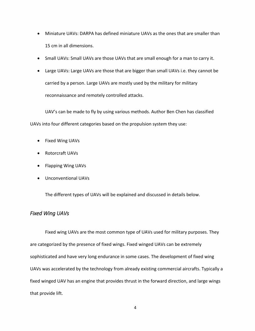
Figure 1-4 NASA Pathfinder (Galante, 2001)

It uses solar energy to charge onboard batteries to operate its flight and avionics. It was

developed by NASA to use as a high altitude/high endurance vehicle for environmental

research. Its wingspan is 29 meters (NASA n.d.)

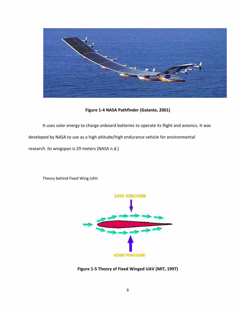
Theory behind Fixed Wing UAV:

Figure 1-5 Theory of Fixed Winged UAV (MIT, 1997)

7

Fixed winged aircraft make use of the difference in pressure created by the camber in

the airfoil (wing). Bernoulli’s equation states that

( 1 )

And Continuity Equation states that

( 2 )

Where,

P=pressure

Ρ= density of the air

V=velocity of the moving air

A= cross sectional area of flow

The surface area of the top of the airfoil is greater than the bottom. When the air

flows over the airflow, assuming the density of the air remains unchanged, the air on the top of

the wing moves faster than the air on the bottom (by Continuity). Since the velocity of the air is

greater on the top, the pressure has to be low (by Bernoulli’s equation). Because there is a

pressure difference on the top and the bottom, there is an upward pressure force applied to

the airfoil (pressure on the top is lower). This creates lift. To move the aircraft forward, the

8

fixed wing aircraft has an engine to provide thrust forward. This thrust has to overcome the

drag provided by air (mit.edu, 1997).

Rotorcraft UAVs

Rotorcrafts are defined as those aircrafts that can fly by the lift created by one or more

rotating blades. Rotorcrafts are very popular in applications such as rescue mission, resupply

mission etc., because of their unique ability to hover, take off and land vertically. Rotorcrafts

are very useful because they can fly to and from any kind of terrain, making them very useful in

emergencies, scientific studies and entertainment industry (eg. aerial filming).

Rotorcrafts ranges from very small (2/3 inches) to big full sized helicopters. Small

rotorcrafts can be designed to be battery operated and whisper quiet increasing its usefulness

in stealth operation. Small rotorcrafts are ideal in confined spaces for example, inside the

buildings and caves (for scientific research or emergency operations) etc.

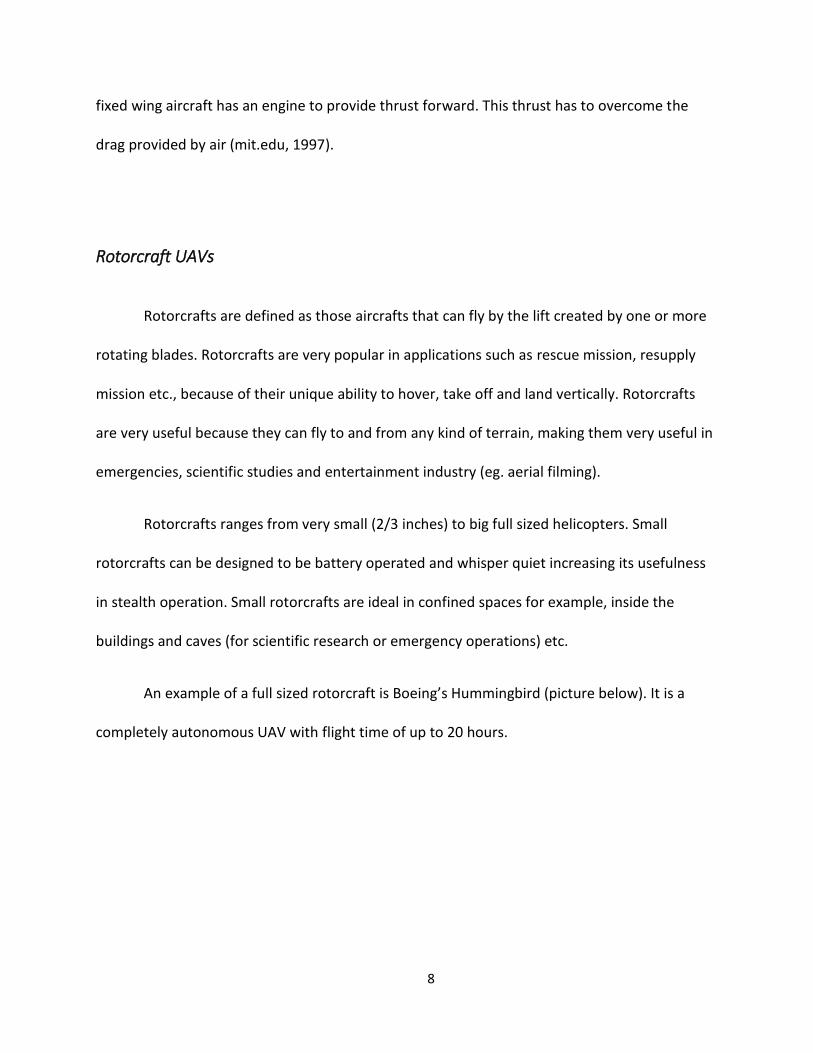
An example of a full sized rotorcraft is Boeing’s Hummingbird (picture below). It is a

completely autonomous UAV with flight time of up to 20 hours.

9

Figure 1-6 Full Sized helicopter UAV called Hummingbird (Trimble, 2009)

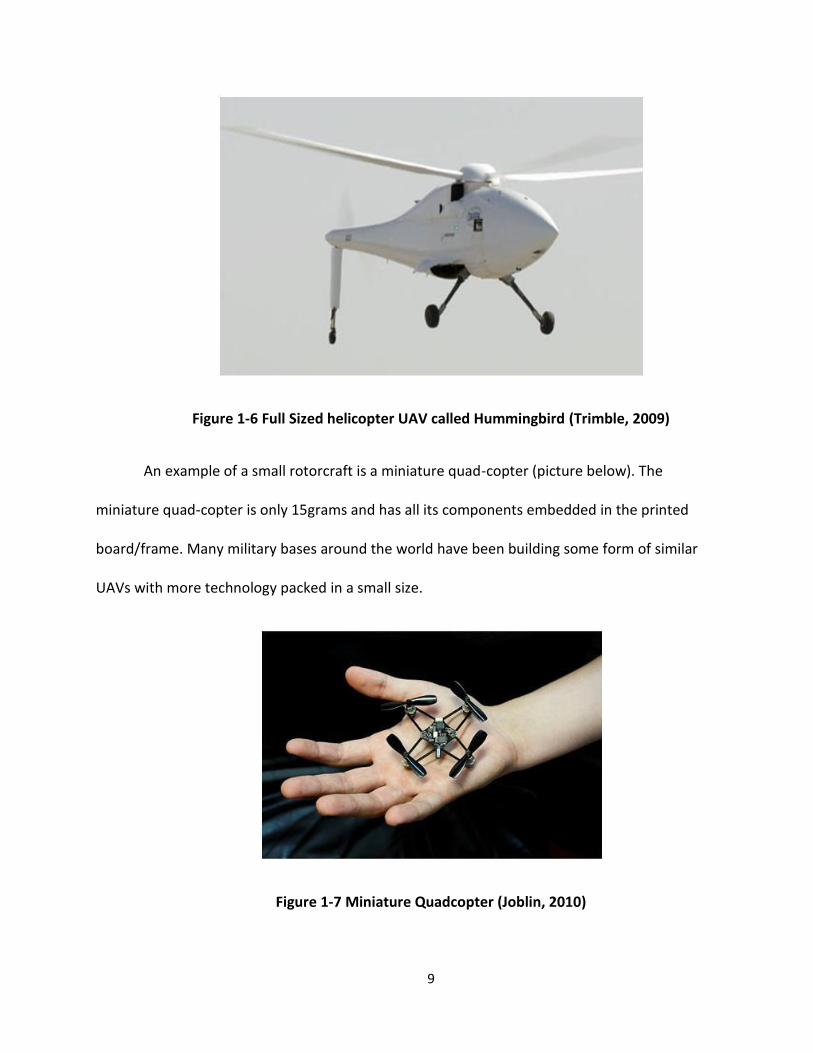
An example of a small rotorcraft is a miniature quad-copter (picture below). The

miniature quad-copter is only 15grams and has all its components embedded in the printed

board/frame. Many military bases around the world have been building some form of similar

UAVs with more technology packed in a small size.

Figure 1-7 Miniature Quadcopter (Joblin, 2010)

10

Theory of Rotorcrafts:

Rotorcrafts use rotors to create lift. Rotors are the blades that are connected to a

rotating shaft. The lifting force created by a rotor can be described by a simple theory called

actuator disc theory (or momentum theory). Actuator Disc Theory states that lift is achieved by

the change in momentum. The Actuator Disc Theory for hovering flight is derived below:

Assumptions: air is incompressible, and the flow is one-dimensional, existence of a

stream-tube which is an asymmetric surface passing through the rotor disc perimeter which

isolates the flow through the rotor.

Figure 1-8 Actuator Disc Theory (Seddon and Newman, 2011)

The flow enters the stream tube, is accelerated through the rotor disc increasing the

velocity and exits the stream-tube. The continuity equation of the flow can be represented by

the following:

11

So, ρAVi = ρAV2 ( 3 )

The rate of change of momentum gives the thrust of the rotors:

T = ρAVi . V2 ( 4 )

Thrust can also be represented in the form of pressure difference as follow:

T = A (pL-pU) ( 5 )

Now by Bernoulli’s equation. Assuming that the velocity of the air in infinite distance

upstream of the rotor is 0, above the rotor, the Bernoulli’s equation takes the form of:

( 6 )

Below the rotor the Bernoulli’s equation looks like

( 7 )

Subtracting these gives:

( 8 )

Since,

T = ρAVi . V2= A (pL-pU) = A

So,

( 9 )

The power of the rotors to produce given thrust can now be written as

12

( 10 )

Flapping Wing UAVs

We human beings have been long intrigued by the way birds fly. In fact when Leonardo

Da-Vinci (1952-1519) made one of the early aircrafts, it was modeled after a bird. Although that

aircraft was not successfully built during that period, modern technology has allowed us to

create an aircraft with flapping wings at present. A flapping Wing UAV is identified as an aircraft

that uses flapping wings as the propulsion system. It may also use airfoil style wings to perform

gliding motion along with the flapping to rise up.

One of the best examples of a flapping wing UAV is the Smart-bird designed by a

German company called Festo (robot bird 2011).

Figure 1-9 Festo Smart-Bird (robot bird, 2011)

13

The Smart-bird can fly just like a real bird, and can be made to look like a read bird when

looking from the bottom, thus can serve as a valuable tool for military intelligence gathering.

Another very good example of a flapping wing UAV is the robot birds being developed in

Wright-Patterson Air Force Base. (Airforce 2012)

Figure 1-10 Robot Bird (Airforce, 2012)

The bird like robot flies by flapping its wings and is designed to use to gather

intelligence. In the picture above the bird is sitting on the wire monitoring the door for

suspicious activity.

14

Unconventional UAV:

A UAV that uses propulsion system other than the fixed wings, rotorcraft or flapping

wings fall under this category. For example people have been using helium (lighter than air) as a

means of flying. Another unconventional flight system is using inversion to fly.

German inventor Paul Schatz has invented a “six-sized articulated rings of prisms that

attached to a cube, and when it is unleashed, it can start unfolding into new geometric shapes.

As it turns inside out, it moves forward. This property of kinematics is called inversion.” The

flying object uses helium to float in the air and inversion to move forward.

Figure 1-11 UAV that uses helium and Inversion technology to fly (Forman, 2012)

15

Ducted fan

A ducted fan or ducted propeller is comprised of two components- the first one is the

fan or propeller. Propeller is a device that converts rotational motion produced by the engine

(or electric motor) into thrust. The second component is the duct. Duct can be defined as a

channel or tube that can be used to convey particularly fluid. Ducts, or shrouds is used along

with the propellers in a UAV for mainly two purposes:

1. It provides protection to the propellers against collision with the wall or contact with

external things including human beings. This protects the propellers, from breaking in

case of a crash or hurting people.

2. Ducts can increase the thrust produced. Most studies suggest that ducts increase the

static thrust produced. If not optimized, the ducts could also lead to excessive losses.

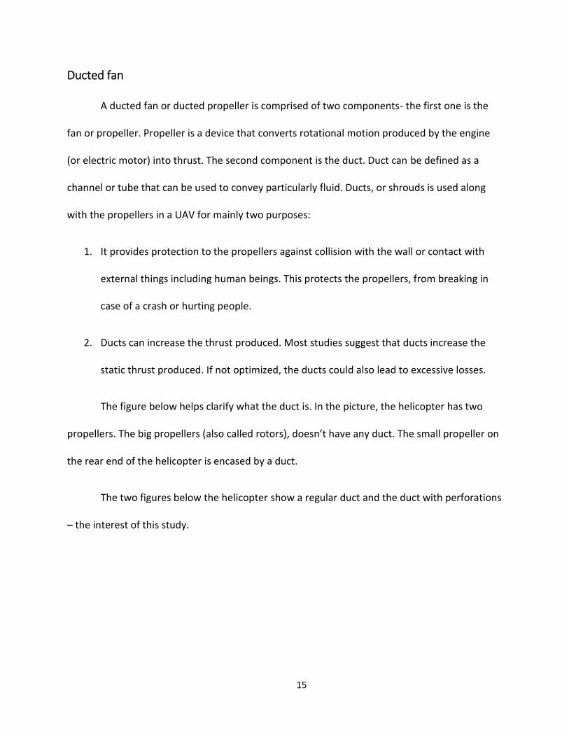
The figure below helps clarify what the duct is. In the picture, the helicopter has two

propellers. The big propellers (also called rotors), doesn’t have any duct. The small propeller on

the rear end of the helicopter is encased by a duct.

The two figures below the helicopter show a regular duct and the duct with perforations

– the interest of this study.

16

Helicopter with both free(un-ducted) and ducted propellers (Piasecki, 2009)

Un-perforated Duct Perforated Duct

Figure 1-12 Examples of un-ducted and ducted propellers, and a perforated duct

Ducts are traditionally known to increase the net thrust produced by the propellers at

high speeds. According to Raphael Yoli the ducts can create up to 30% more thrust over free

propellers for some optimized conditions.

From a scientific study conducted by NASA on ducted rotors, it was found out that the

Ducts increase the thrust in higher RPMs (>4000) of propellers. In relatively lower RPMs

however, there were more losses due to the addition of duct (high internal duct drag). It was

also found from the same study that as the tip gap was reduced, some gain in thrust was seen

even in smaller RPMs (Martin,2004). Please note that the study doesn’t relate RPM with

Ducted Propeller

Free Propeller

17

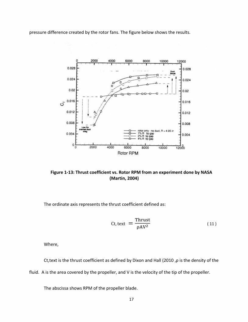
pressure difference created by the rotor fans. The figure below shows the results.

Figure 1-13: Thrust coefficient vs. Rotor RPM from an experiment done by NASA (Martin, 2004)

The ordinate axis represents the thrust coefficient defined as:

( 11 )

Where,

Ct,text is the thrust coefficient as defined by Dixon and Hall (2010 ,ρ is the density of the

fluid. A is the area covered by the propeller, and V is the velocity of the tip of the propeller.

The abscissa shows RPM of the propeller blade.

18

In Figure 1-13, the ducts start showing increased thrust only after the propeller speed is

faster than 4000 RPM. This transition speed changes depending upon the duct material, the size

of the rotor, tip gap etc.

Motivation

Ducted propellers can be essential to some UAVs more than others. Take for example

Incredible HLQ from Figure 1. In such rescue UAVs that needs to operate in confined or

crowded areas, a duct may be necessary for public safety and the UAV’s own safety.

Additionally, ducted propellers are known to increase the efficiency up to 30% as compared to

a free propeller (Martin, 2004). In a study performed in 2004 by NASA scientists, ducted

propellers provided higher static thrust than free propellers in high RPM of the propeller.

However the thrust was found to be lower in ducted propellers in low RPM Speed. As it is

obvious, addition of duct increases the overall weight of the vehicle. Added weight can be a

huge penalty for small UAVs which already have a small weight. Please note that the 30%

increase in static thrust as calculated by NASA scientists didn’t take into account the weight of

the duct. It will be interesting to find out if there is any net thrust gain when the weight of duct

is included for comparison. While ducted rotors can increase the thrust produced, it also adds

weight to the UAV. It was therefore hypothesized that by removing part of the duct materials

(i.e. adding perforations in the duct) would benefit from both decreased duct weight and

increased thrust. However, it is not clear how much trade-off would be between these two

factors. The motivation of this study is to find out if optimization in thrust is possible by using

perforated ducts.

19

Objectives

The objectives of this study are:

1. Explore how the net thrust changes in small UAVs with ducted propeller when the

weight of the duct in included in net thrust calculation at different RPM speeds.

2. Explore how addition of perforations in the duct affects the thrust at various RPM speed

of the propellers by using commercial computational fluid dynamics software Ansys/

Fluent.

Approach

The study was done mostly using Fluent and ICEM CFD software. The real conditions

were simulated as closely as possible in the software and the case solved in the software. The

first step was to learn the software. This phase of study was called CFD training and literature

research period. Once the software was learnt, some simple cases such as pipe flow and

channel flow were ran as they had easily available analytical solutions to compare the results

from the Fluent to the analytical data. This was done to be proficient in modeling, and software

usage. Next the cases without duct, with duct, and different size of perforations were done.

Thrust was calculated using conservation of momentum equation. At the end useful

conclusions were drawn from the results.

20

Chapter 2 : SOFTWARE TRAINING

The study presented in this study relies heavily on the Computational Fluid Dynamics (CFD)

software called Fluent and the related meshing software called ICEM-CFD. Some very simple cases were

studied and compared to their corresponding analytical solutions to verify the usefulness of software,

and the accuracy of the results. Two of the many cases done are presented below to provide the

examples of cases studied for training. Details of all the cases are available in the appendix.

Case 1: Laminar Channel Flow

Problem Statement:

Figure 2-1 Problem Statement for Laminar channel flow

As shown in the figure above, air flows into the pipe at a uniform velocity of 0.3032 m/s and

exits at atmospheric pressure.

Density used (ρ): 1.204 kg/m^3

Dynamic Viscosity (µ): 1.825 * 10^-5 kg/ (m-s)

Reynold’s number based on the diameter = ReD = 200

21

Solving Navier’s Stokes Equations, it can be proved that,

The problem was solved in Fluent. The fully developed velocity profiles are compared as follows:

Figure 2-2 x-velocity vs. y-coordinate for laminar channel flow

The average velocity of the fully developed flow is 0.3032 m/s. From the graph above, the

maximum velocity is expected to be around 0.45 m/s. The maximum velocity as obtained from the

Fluent’s solution is about 1.53% off of the ideal solution. The error mainly comes from lack of enough

grid points.

The skin friction coefficient is plotted in the figure below showing that the skin friction

coefficient remains constant once the flow is fully developed.

0

0.002

0.004

0.006

0.008

0.01

0.012

0 0.1 0.2 0.3 0.4 0.5

He

igh

t o

f C

han

ne

l (m

)

x-velocity (m/s)

x-velocity vs y-coordinate

Ideal

FLuent

22

Figure 2-3 skin Friction coefficient for laminar channel flow

0.2, 0.0581784

0.04

0.045

0.05

0.055

0.06

0.065

0.07

0.075

0.08

0 0.05 0.1 0.15 0.2 0.25

Skin

Fri

ctio

n C

oe

ffic

ien

t

X-coordinate (m)

Skin Friction Coefficient

Skin Friction Coefficient

23

Case 2: Laminar Pipe Flow with a constant heat flux at the surface

Problem Statement:

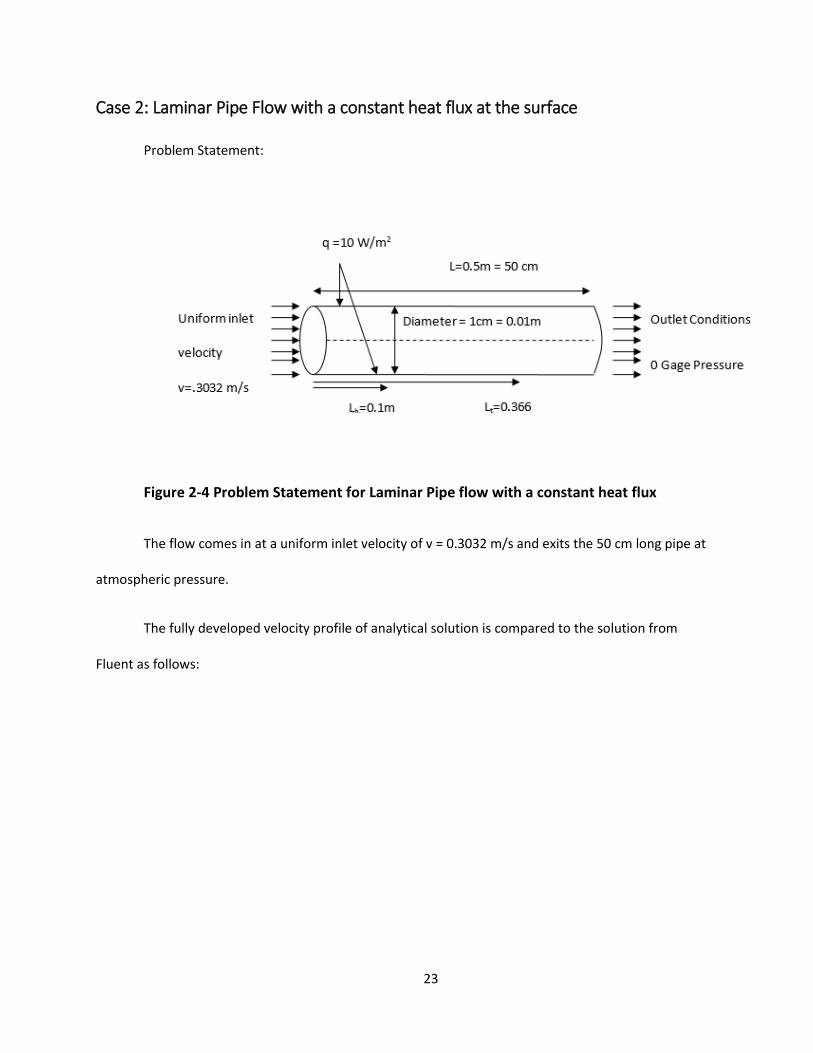
Figure 2-4 Problem Statement for Laminar Pipe flow with a constant heat flux

The flow comes in at a uniform inlet velocity of v = 0.3032 m/s and exits the 50 cm long pipe at

atmospheric pressure.

The fully developed velocity profile of analytical solution is compared to the solution from

Fluent as follows:

24

Figure 2-5 Ideal velocity vs. velocity profile obtained from fluent

As can be see, the solution from fluent was only 2.4% away from the analytical solution.

Figure 2-6 skin friction coefficient vs x-coordinate

The skin friction coefficient remains constant after a certain distance.

0

0.002

0.004

0.006

0.008

0.01

0.012

0 0.2 0.4 0.6 0.8

r (m

)

Velocity (m/s)

Ideal velocity vs. Fluent's velocity Profile

Ideal velocity Profile

Fluent Velocity Profile

0

0.2

0.4

0.6

0.8

1

1.2

0 0.2 0.4 0.6

Skin

Fri

ctio

n C

oe

ffic

ien

t

X-Coordinate (m)

SkinFrictionCoefficient vs X-Coordinate (f=0.039244)

SkinFrictionCoefficient vs X-Coordinate

25

Figure 2-7 Development of Dimensionless Temperature profile

The dimensionless temperature profile develops to be fully developed as shown in the figure

above.

Figure 2-8 Variation of Nusselt's number with x-coordinate

The Nusselts number remains constant after a while.

0

0.002

0.004

0.006

0.008

0.01

0.012

0 0.5 1 1.5 2

Rad

ial D

ista

nce

(m

)

Dimensionless Temperature

Development of Dimensionless Temperature Profile

Dimensionless Temp (x=0.1) vs Y

Dimension Temp at (x=0.5)

0

1000

2000

3000

4000

5000

6000

0 0.2 0.4 0.6

Nu

sse

lt's

Nu

mb

er

Distance from the entrance (m)

X-coordinate vs Surface Nusselts number

X-coordinate vs Surface Nusselts number

26

Chapter 3 : THEORY

Thrust is defined as the upward force applied to the UAV, because of the momentum changed

created by the propeller. To calculate Thrust, Momentum conservation equation was applied to all the

surface surrounding the control volume. It is defined in much detail in the following sections.

Formulation of Momentum Equation:

The conservation of Momentum Equation (Newton’s Second law) states that the force is equal

to the rate of momentum change.

(3.1)

Where, P = Linear Momentum

Sys = system (Fixed Mass)

Before moving on, defining control volume and control mass (system) is deemed necessary.

System is any closed space, from which no mass particles is leaving or coming in. In other words,

the mass of a system is constant. Eg. The air inside a soccer ball can be taken as a system, because there

is no mass loss to the surrounding.

On the other hand, a control volume is any volume which is allowed to exchange both mass and

energy to its surrounding. Eg. The volume around a turbine is a control volume.

For a fluid control volume, this equation for a system is related to the equation for a control

volume by using Reynold’s Transport Theorem, which states that:

27

(3.2)

Where,

B = conserved quantity

= conserved quantity per unit mass

In our case, the conserved quantity is Momentum, set B = P = , which makes =

Hence the Reynolds’s transport equation can now be written as:

(3.3)

Force = Rate of Change of Momentum = Rate of change of momentum within CV + Rate of

Momentum Flux (Martin and Tung, Performance and Flowfield Measurements on a 10-inch Ducted

Rotor VTOL UAV 2004)

Applying Momentum Equation to the Propeller without the duct:

An arbitrary control volume is created around the propellers and the Conservation of

Momentum Equation is applied around it.

28

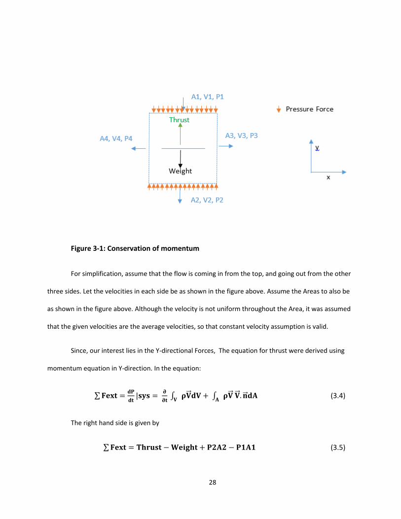
Figure 3-1: Conservation of momentum

For simplification, assume that the flow is coming in from the top, and going out from the other

three sides. Let the velocities in each side be as shown in the figure above. Assume the Areas to also be

as shown in the figure above. Although the velocity is not uniform throughout the Area, it was assumed

that the given velocities are the average velocities, so that constant velocity assumption is valid.

Since, our interest lies in the Y-directional Forces, The equation for thrust were derived using

momentum equation in Y-direction. In the equation:

(3.4)

The right hand side is given by

(3.5)

29

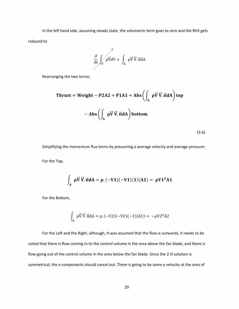
In the left hand side, assuming steady state, the volumetric term goes to zero and the RHS gets

reduced to

Rearranging the two terms:

(3.6)

Simplifying the momentum flux terms by presuming a average velocity and average pressure:

For the Top,

For the Bottom,

For the Left and the Right, although, It was assumed that the flow is outwards, it needs to be

noted that there is flow coming in-to the control volume in the area above the fan blade, and there is

flow going out of the control volume in the area below the fan blade. Since the 2-D solution is

symmetrical, the x-components should cancel out. There is going to be some y-velocity at the area of

30

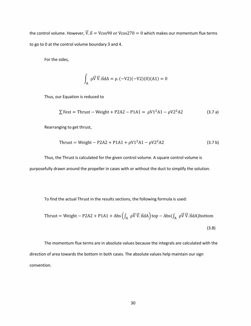
the control volume. However, which makes our momentum flux terms

to go to 0 at the control volume boundary 3 and 4.

For the sides,

Thus, our Equation is reduced to

(3.7 a)

Rearranging to get thrust,

(3.7 b)

Thus, the Thrust is calculated for the given control volume. A square control volume is

purposefully drawn around the propeller in cases with or without the duct to simplify the solution.

To find the actual Thrust in the results sections, the following formula is used:

(3.8)

The momentum flux terms are in absolute values because the integrals are calculated with the

direction of area towards the bottom in both cases. The absolute values help maintain our sign

convention.

31

Modified Thrust Coefficient

Since rotor tip velocity is not available to us to define thrust coefficient as many text books do,

the thrust Coefficient used in the results is redefined as:

(3.9)

Where,

Ct is the thrust coefficient, , A is the cross sectional area of the

disc(that replaces propellers), and V is the maximum velocity of the air in the control volume.

Efficiency of Duct

The efficiency of the ducted fan is given by:

Efficiency (η) =

Thrust output is the net thrust (including the duct weight) obtained. Pressure Force in is

the pressure that is put in as input in the fan blade. The Pressure Force In is calculated as

Pressure force in = ΔP * A

ΔP is the Pressure difference that is input in the fan boundary conditions, and A is the surface

area of the infinitely thin Disc that is creating the discontinuous pressure difference.

32

Navier-Stokes Equations

Conservation of momentum can also be written using Navier-stokes Equations. For an

infinitesimally small moving fluid element, the forces applied in the x-direction can be

represented as the figure below. The forces applied to the body are pressure forces, and the

viscous (shear and normal shear) forces. Starting out with F=ma in each of the three Cartesian

directions, and with some modifications (similar to the one in thrust calculation section above)

the Navier-Stokes Equations is obtained. The detailed derivation can be easily found in any

Fluids or CFD text book (eg. Anderson’s CFD). Fluent uses these three equations to solve for

unknown quantities.

Figure 3-2 Forces in x-direction in an infinitesimally small, moving fluid element (Anderson CFD)

33

The Navier Stokes Equations (Munson, Young and Okiishi 2008)is given as:

(3.10)

34

Chapter 4 : MODELING AND SIMULATION OF AIRFLOW

3-D propeller to 2-D Disc

To study the effects created by a rotating propellers, a 3-D model of the propellers is

ideal. However 3-D modeling is arduous and very time consuming. As an example, solving a 2-D

duct with close to half a million grid points took close to 30 hours to converge. A 3-D study

would have taken much longer. Secondly, the educational version of Ansys Fluent used for this

study did not allow the number of grid points that would have been required for a 3-D

propellers and duct. The main advantage of a 3-D model is much better swirl modeling.

However, swirl was neither under the scope of this study nor did it greatly affect the thrust.

Hence, the study was done in 2-D.

One major challenge was to reduce a 3-Dimensional propeller to 2-D. This was

accomplished by using infinitely thin Disc (rotor disc). The thin disk creates discontinuous

pressure change through it.

35

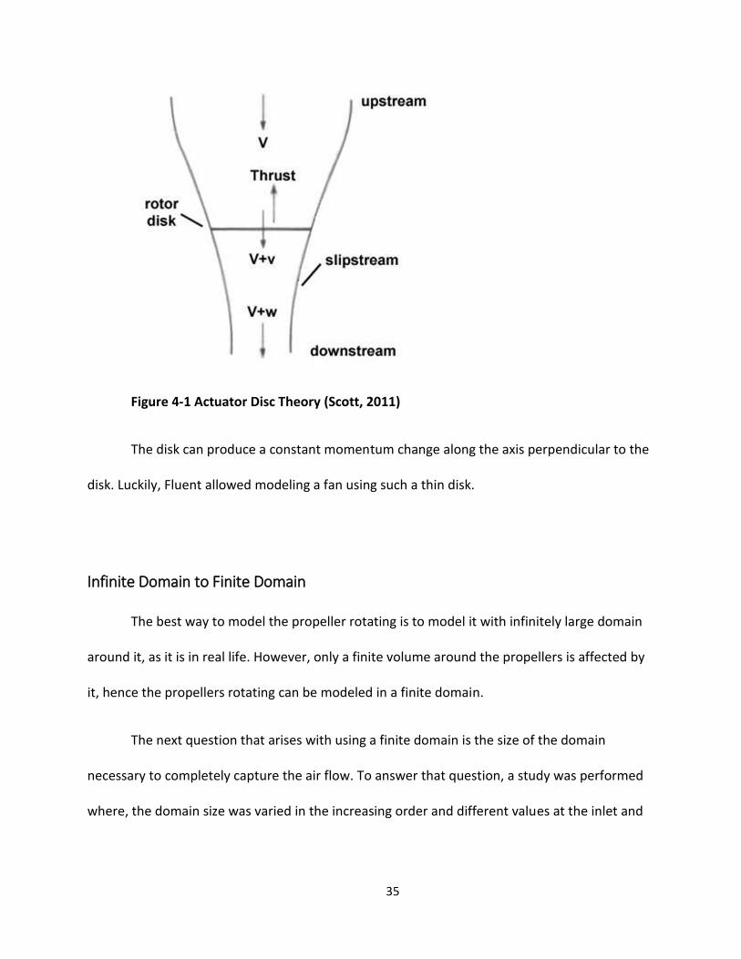
Figure 4-1 Actuator Disc Theory (Scott, 2011)

The disk can produce a constant momentum change along the axis perpendicular to the

disk. Luckily, Fluent allowed modeling a fan using such a thin disk.

Infinite Domain to Finite Domain

The best way to model the propeller rotating is to model it with infinitely large domain

around it, as it is in real life. However, only a finite volume around the propellers is affected by

it, hence the propellers rotating can be modeled in a finite domain.

The next question that arises with using a finite domain is the size of the domain

necessary to completely capture the air flow. To answer that question, a study was performed

where, the domain size was varied in the increasing order and different values at the inlet and

36

exit of the duct were monitored. The monitored values are y-momentum flux, and Area

weighted average pressure.

All of the domain sizes were rectangular. The four sizes are shown below. Different

colors represent different sizes. Duct is always at the center in the x-axis so has not been shown

in the figures. The Duct size has been exaggerated.

37

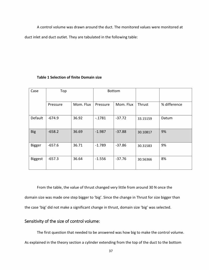
A control volume was drawn around the duct. The monitored values were monitored at

duct inlet and duct outlet. They are tabulated in the following table:

Table 1 Selection of finite Domain size

Case Top Bottom

Pressure Mom. Flux Pressure Mom. Flux Thrust % difference

Default -674.9 36.92 -.1781 -37.72 33.15159 Datum

Big -658.2 36.69 -1.987 -37.88 30.10817 9%

Bigger -657.6 36.71 -1.789 -37.86 30.31583 9%

Biggest -657.3 36.64 -1.556 -37.76 30.56366 8%

From the table, the value of thrust changed very little from around 30 N once the

domain size was made one step bigger to ‘big’. Since the change in Thrust for size bigger than

the case ‘big’ did not make a significant change in thrust, domain size ‘big’ was selected.

Sensitivity of the size of control volume:

The first question that needed to be answered was how big to make the control volume.

As explained in the theory section a cylinder extending from the top of the duct to the bottom

38

of the duct was choosen as the control volume. The next question that needed to be answered

was what to take as the diameter of the cylinder. A study was conducted a study to see how

changing diameter of the cylinder would change the thrust calculated. Our smallest diameter

was the diameter of the duct which is 0.127 m, and the largest diameter was 0.3 m. The

cylinder and the duct had coincident central axis. The results of the study is shown below. The

datum was the Thrust calculated by using the diameter of the Duct.

Diamter Thrust Remarks

%

change

Duct

with no

pores

0.254 275.687 Datum 0%

0.3 276.5809 0%

0.4 278.7078 1%

0.6 272.2305 1%

No

Duct

0.254 274.3788 Datum 0%

0.3 290.7763 6%

0.4 297.6186 8%

0.5 293.4466 7%

0.6 292.8267 7%

Table 2 Sensitivity of the diameter of the control volume cylinder

From the table above, the sensitivity is very low for the duct; however it is pretty

significant in the case with no duct. The thrust increases significantly when the diameter is

increased from 0.127 m to 0.15 meters.

To calculate the thrust, the diameter of the cylinder was usually taken around 1.18-0.2

m, so that the maximum thrust provided by the rotors is captured. In calculating thrust for each

39

section, various diameters from 0.16-0.22 were tried, and the highest thrust producing

diameter was selected.

This creates a source of inconsistency when comparing two thrusts, but this

inconsistency was removed by using modified thrust coefficient.

Wall Functions

The wall functions in fluent are used to model the turbulent flow very close to the wall.

Using wall functions allows fluent users to not have to create very fine mesh next to the wall.

Wall function are usually determined by y-plus value. Y-plus value is the value calculated using

the flow conditions that dictate how close the first mesh has to be to the wall. For accurate

results when using standard wall functions, the y-plus value has to be around 30 – 200, closer

you are to 30 the better. For all our meshes, y-plus value around the duct varied anywhere from

mid 40s to ~160. Y+ values were calculated using the inbuilt y-plus calculator in Fluent.

Pressure inlet/outlet Boundary Conditions:

Fluent didn’t have detailed definition of what different boundary conditions meant. To

make sure, correct boundary condition was selected a study was done to verify the different

boundary conditions. One boundary condition that wasn’t well defined in the manual was

pressure inlet/outlet boundary condition. To solve this conundrum, the case without duct was

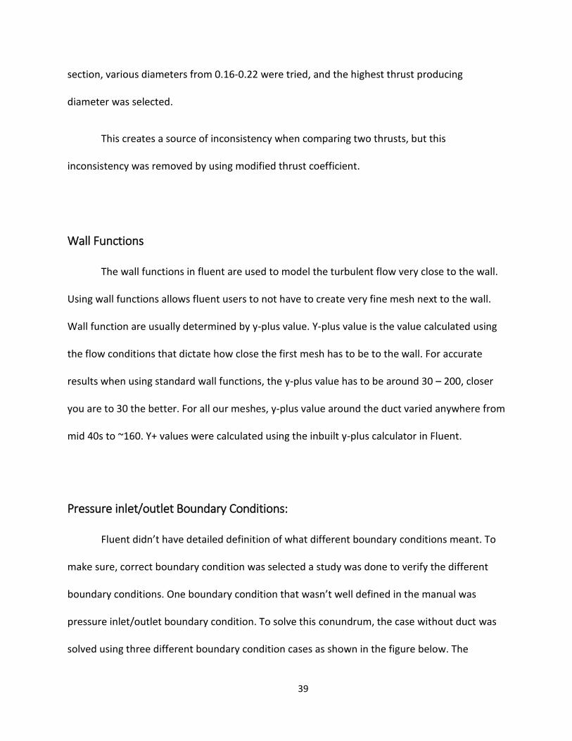
solved using three different boundary condition cases as shown in the figure below. The

40

pressure difference created by the disc blade was set to 3000 Pa. All the boundary conditions

were 0 gage pressure. The results showed us that for our cases there is no difference in the

results obtained by using either pressure inlet or outlet conditions. They meant the same thing.

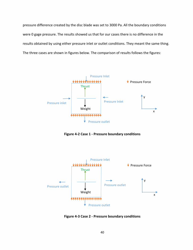
The three cases are shown in figures below. The comparison of results follows the figures:

Figure 4-2 Case 1 - Pressure boundary conditions

Figure 4-3 Case 2 - Pressure boundary conditions

Pressure Inlet

Thrust

Weight

Pressure Force

y

x

Pressure Inlet Pressure inlet

Pressure outlet

Pressure Inlet

Thrust

Weight

Pressure Force

y

x

Pressure outlet Pressure outlet

Pressure outlet

41

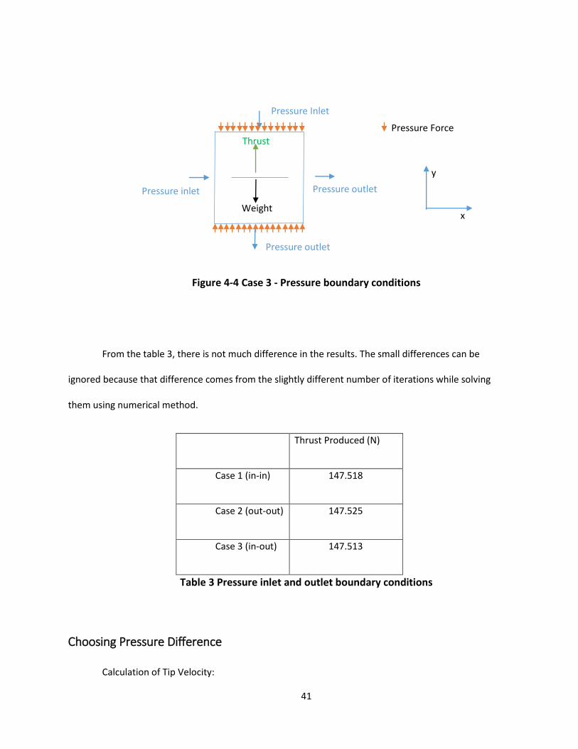
Figure 4-4 Case 3 - Pressure boundary conditions

From the table 3, there is not much difference in the results. The small differences can be

ignored because that difference comes from the slightly different number of iterations while solving

them using numerical method.

Thrust Produced (N)

Case 1 (in-in) 147.518

Case 2 (out-out) 147.525

Case 3 (in-out) 147.513

Table 3 Pressure inlet and outlet boundary conditions

Choosing Pressure Difference

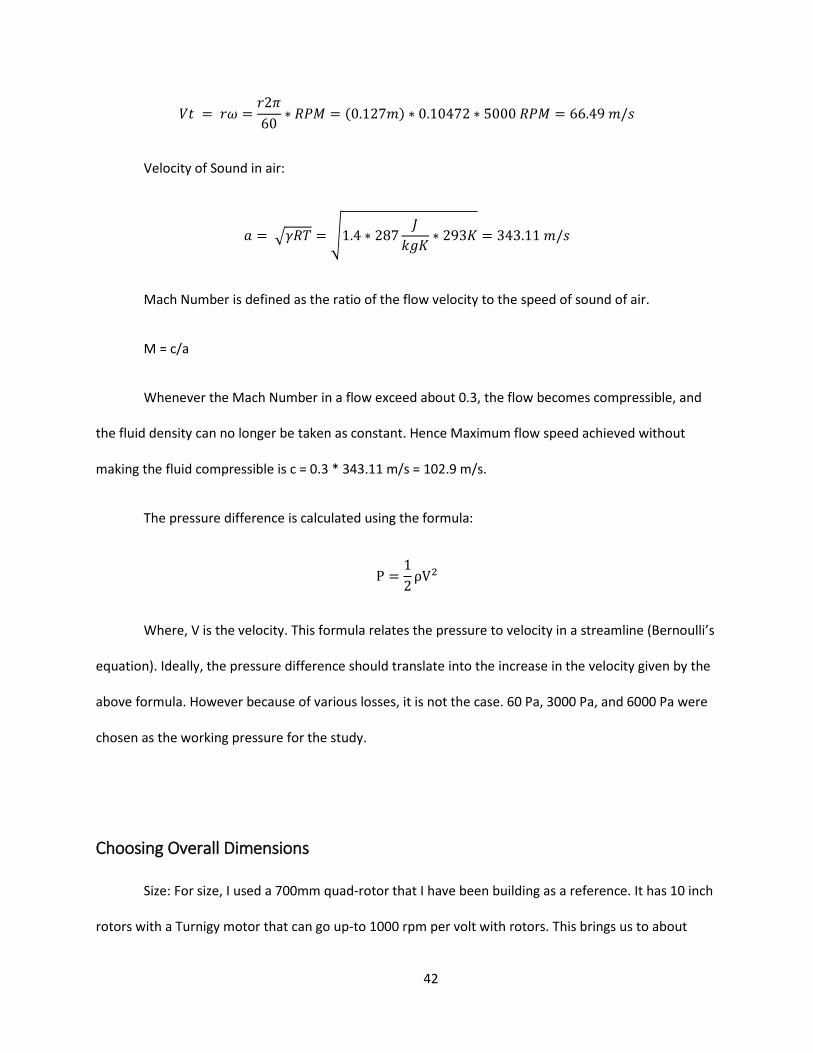
Calculation of Tip Velocity:

Pressure Inlet

Thrust

Weight

Pressure Force

y

x

Pressure outlet Pressure inlet

Pressure outlet

42

Velocity of Sound in air:

Mach Number is defined as the ratio of the flow velocity to the speed of sound of air.

M = c/a

Whenever the Mach Number in a flow exceed about 0.3, the flow becomes compressible, and

the fluid density can no longer be taken as constant. Hence Maximum flow speed achieved without

making the fluid compressible is c = 0.3 * 343.11 m/s = 102.9 m/s.

The pressure difference is calculated using the formula:

Where, V is the velocity. This formula relates the pressure to velocity in a streamline (Bernoulli’s

equation). Ideally, the pressure difference should translate into the increase in the velocity given by the

above formula. However because of various losses, it is not the case. 60 Pa, 3000 Pa, and 6000 Pa were

chosen as the working pressure for the study.

Choosing Overall Dimensions

Size: For size, I used a 700mm quad-rotor that I have been building as a reference. It has 10 inch

rotors with a Turnigy motor that can go up-to 1000 rpm per volt with rotors. This brings us to about

43

5000 rpm in a 5Volt Power source. The max rated power is 730 (HobbyKing 2013). Hence 10-inch rotors

were used to get a realistic feel.

Perforations

Many different perforations were chosen to be compared. The perforations were

increased to increase the open area %, which went from 0% open area for duct with no pores

to 100% area for propellers without duct. Each perforation is explained by using figures below.

1. 0% Open Area: This configuration has no open area, i.e. complete duct. The duct has no

perforations included.

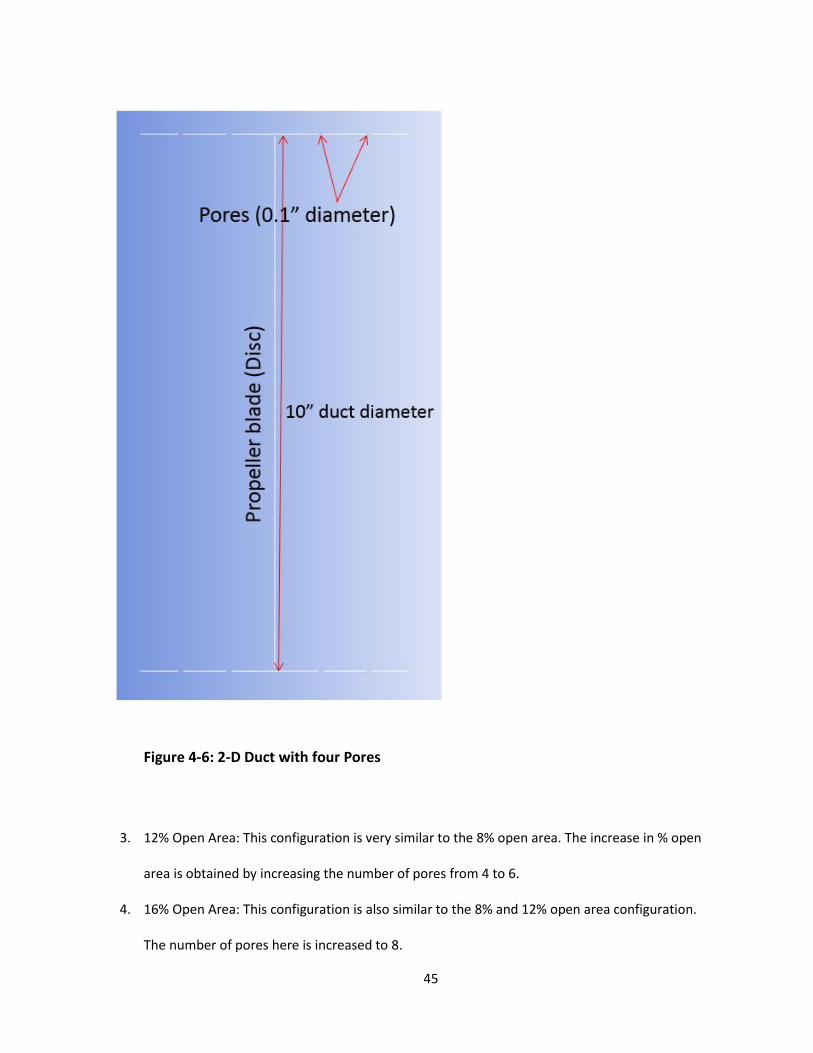
2. 8% Open Area: This configurations has 4 0.1” pores on the duct, two are above the

propeller disc and two are below the disc as shown in the figures below. From the solid

model(Figure 4-5), the pores created in 2-D translate to a duct with continuous open

area. Although this is unrealistic and the real model would rather have scattered pores,

our only concern is the trends in thrust, and this model provides accurate enough

44

information on the trends.

Figure 4-5: 3-D Translation of an axis-symmetrical plane with 4 Pores

45

Figure 4-6: 2-D Duct with four Pores

3. 12% Open Area: This configuration is very similar to the 8% open area. The increase in % open

area is obtained by increasing the number of pores from 4 to 6.

4. 16% Open Area: This configuration is also similar to the 8% and 12% open area configuration.

The number of pores here is increased to 8.

46

5. 24% Open Area: To create a more realistic situation with the perforations, the pore diameter

was increased to 0.3”. This configuration has 4 pores on each side.

6. 36% Open Area: This also belongs to the family of 24%, but has 6 Pores.

7. 48% Open Area: This configuration has 6 pores on each side, the pores are 0.3” in diameter.

8. 40% Open Area: This configuration was created with 0.5” diameter pores. It has 4 pores.

9. 60% Open Area: 0.5” diameter pores, 6 pores

10. 80% Open Area: 8 0.5” diameter pores.

11. Tiniest Duct: This configurations has a very small duct surrounding it. The size of the duct is 1”.

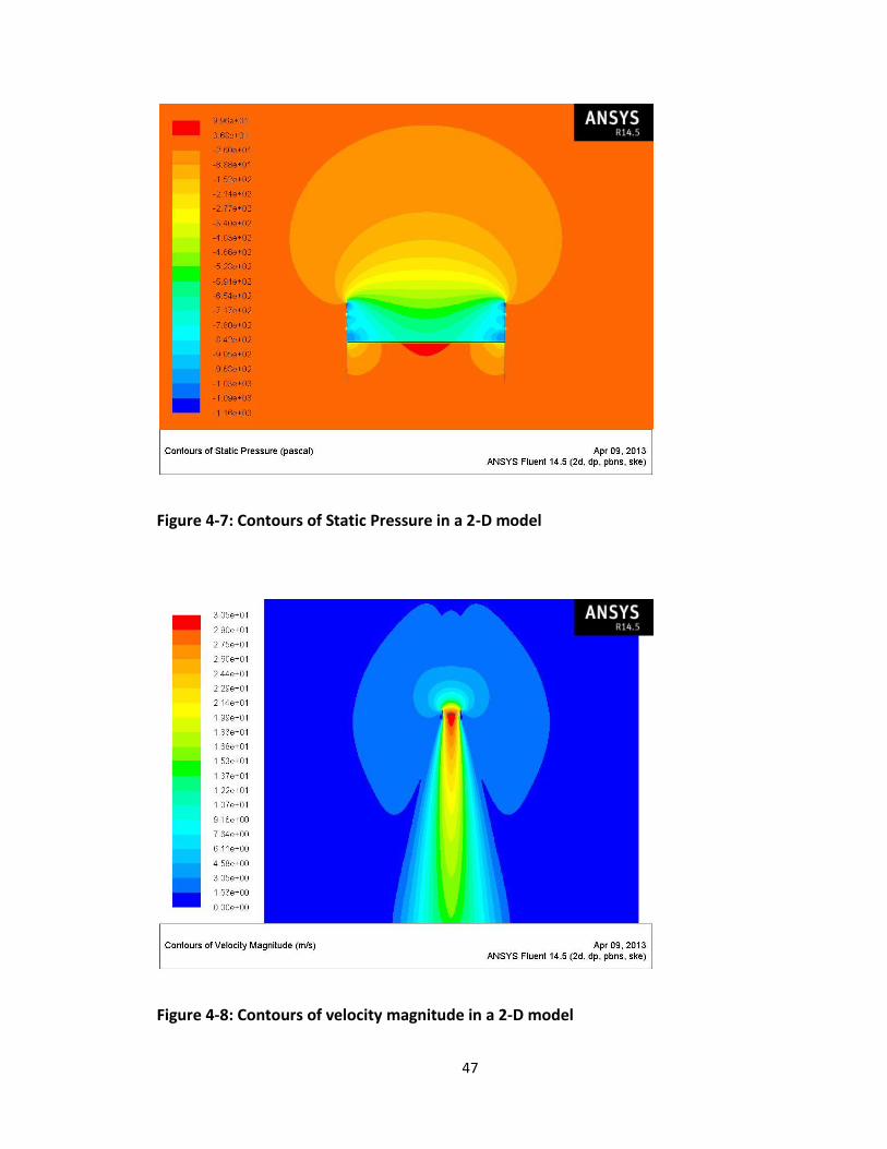
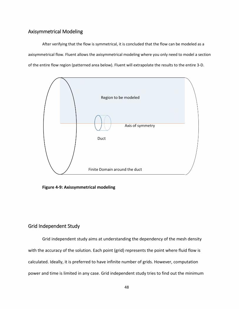
Verification of Symmetry: 2-D Modeling

The study of the ducts was done in 2-dimensional using axisymmetrical model.

However, to verify the symmetry of the flow, a 2-D model of the duct, (as seen in figure above)

that extended 1m behind the screen/paper was devised. The contour plots of the velocity and

pressure is given below. It can be seen that both the velocity and the pressure are symmetrical

in 2-D. This gave us a confirmation that the duct flow can be simulated using an axisymmetrical

model. From the figures below, it is clear that both the pressure and the velocity are

symmetrical.

47

Figure 4-7: Contours of Static Pressure in a 2-D model

Figure 4-8: Contours of velocity magnitude in a 2-D model

48

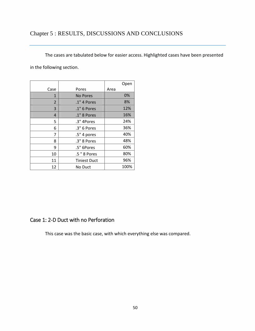
Axisymmetrical Modeling

After verifying that the flow is symmetrical, it is concluded that the flow can be modeled as a

axisymmetrical flow. Fluent allows the axisymmetrical modeling where you only need to model a section

of the entire flow region (patterned area below). Fluent will extrapolate the results to the entire 3-D.

Figure 4-9: Axissymmetrical modeling

Grid Independent Study

Grid independent study aims at understanding the dependency of the mesh density

with the accuracy of the solution. Each point (grid) represents the point where fluid flow is

calculated. Ideally, it is preferred to have infinite number of grids. However, computation

power and time is limited in any case. Grid independent study tries to find out the minimum

49

number of grid points necessary without sacrificing much accuracy. Our main limitation on Grid

is 500000, because student version of Fluent was used to solve the flow. However, 500,000 is a

lot of grids, and our flow is fairly simple. Additionally, since an axis symmetric model is used,

our computational domain is reduced to half. Thus the maximum grid number chosen was

370k.

In reducing the grid points from the maximum grid points, everything was reduced in

proportion. For example, the ratio of number of nodes in each section was kept almost same.

The result of the grid independent study was that the mesh density that was the ideal

was more than enough. However, the maximum number of grids was selected because

computer resources were available.

Table 4 Grid Independent Study for case 5

Bottom Top

Number of Grid Points

Pressure Force

Mom. Flux

Pressure Force

Mom. Flux

Upward Pressure Force Momentum Flux Thrust

370 k 0.528 -297.962 -142.599 -157.909 -143.128 -140.052 -283.180

150 k 0.699 -301.557 -141.693 -161.213 -142.391 -140.345 -282.736

80 k 0.657 -302.131 -139.480 -159.475 -140.138 -142.657 -282.795

50

Chapter 5 : RESULTS, DISCUSSIONS AND CONCLUSIONS

The cases are tabulated below for easier access. Highlighted cases have been presented

in the following section.

Case Pores Open

Area

1 No Pores 0%

2 .1" 4 Pores 8%

3 .1" 6 Pores 12%

4 .1" 8 Pores 16%

5 .3" 4Pores 24%

6 .3" 6 Pores 36%

7 .5" 4 pores 40%

8 .3" 8 Pores 48%

9 .5" 6Pores 60%

10 .5 " 8 Pores 80%

11 Tiniest Duct 96%

12 No Duct 100%

Case 1: 2-D Duct with no Perforation

This case was the basic case, with which everything else was compared.

51

Figure 5-1 Case 1: Duct with no perforations - velocity vectors overlayed on pressure

contour

If the figure above, the velocity vectors are overlaid on the Pressure Contour. The air

comes in from the Top (left side), and passes through the duct. Looking closely at the area

around the blades, it can be found that there is some tip loss, i.e. some air travels backwards

through the tip gap. This creates a recirculation zone next to the tip gap.

FLOW

52

Figure 5-2 Recirculation near tip gap

In the figure above, it can be clearly seen that there is recirculation in two places. First is

right above the fan. The second region is upstream from the fan. There is another flow

separation (recirculation) going on below the duct inlet. This is caused by the shape of the duct

inlet.

Air Flows backwards

through tip gap

53

2-D Duct with 4 Perforations

In this case, duct had 4 perforations on each side, 2 on top of the blade and 2- on bottom of the

blade. The picture below shows us that, there isn’t too much going on most of the domain. The pressure

gradient is higher closer to the duct. This was observed in all cases.

Figure 5-3 Contours of Static pressure - case 2

Significant velocity vectors, however can be noticed even far away from the duct as

shown

54

Figure 5-4 velocity vectors - case 1

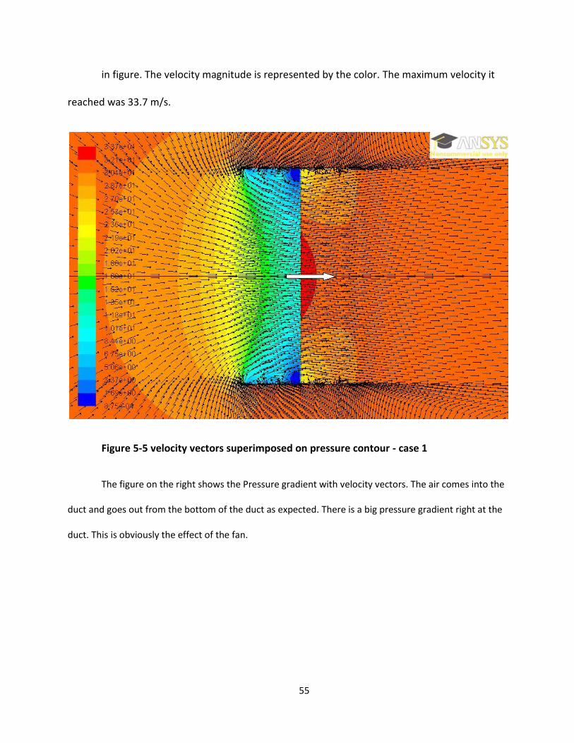
55

in figure. The velocity magnitude is represented by the color. The maximum velocity it

reached was 33.7 m/s.

Figure 5-5 velocity vectors superimposed on pressure contour - case 1

The figure on the right shows the Pressure gradient with velocity vectors. The air comes into the

duct and goes out from the bottom of the duct as expected. There is a big pressure gradient right at the

duct. This is obviously the effect of the fan.

56

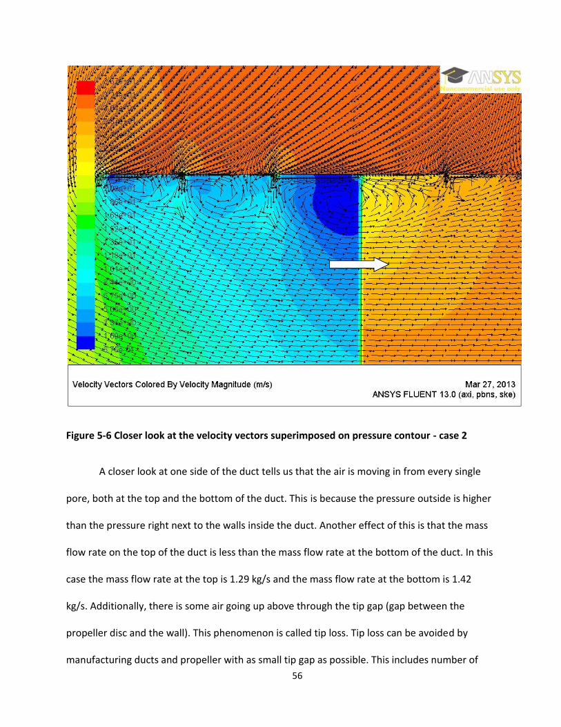
Figure 5-6 Closer look at the velocity vectors superimposed on pressure contour - case 2

A closer look at one side of the duct tells us that the air is moving in from every single

pore, both at the top and the bottom of the duct. This is because the pressure outside is higher

than the pressure right next to the walls inside the duct. Another effect of this is that the mass

flow rate on the top of the duct is less than the mass flow rate at the bottom of the duct. In this

case the mass flow rate at the top is 1.29 kg/s and the mass flow rate at the bottom is 1.42

kg/s. Additionally, there is some air going up above through the tip gap (gap between the

propeller disc and the wall). This phenomenon is called tip loss. Tip loss can be avoided by

manufacturing ducts and propeller with as small tip gap as possible. This includes number of

57

considerations such as expansion of the duct and the propeller due to temperature rise,

accuracy in manufacturing processes etc. In some highly sophisticated turbo machinery, the tip

gap is as small as fractions of an inch.

2-D Duct with 6 Pores:

Just Like the case discussed above, the pressure gradients were abundant near the duct, and not

too much in the rest of the domain.

Figure 5-7 Case 3 - velocity vectors on pressure contour

58

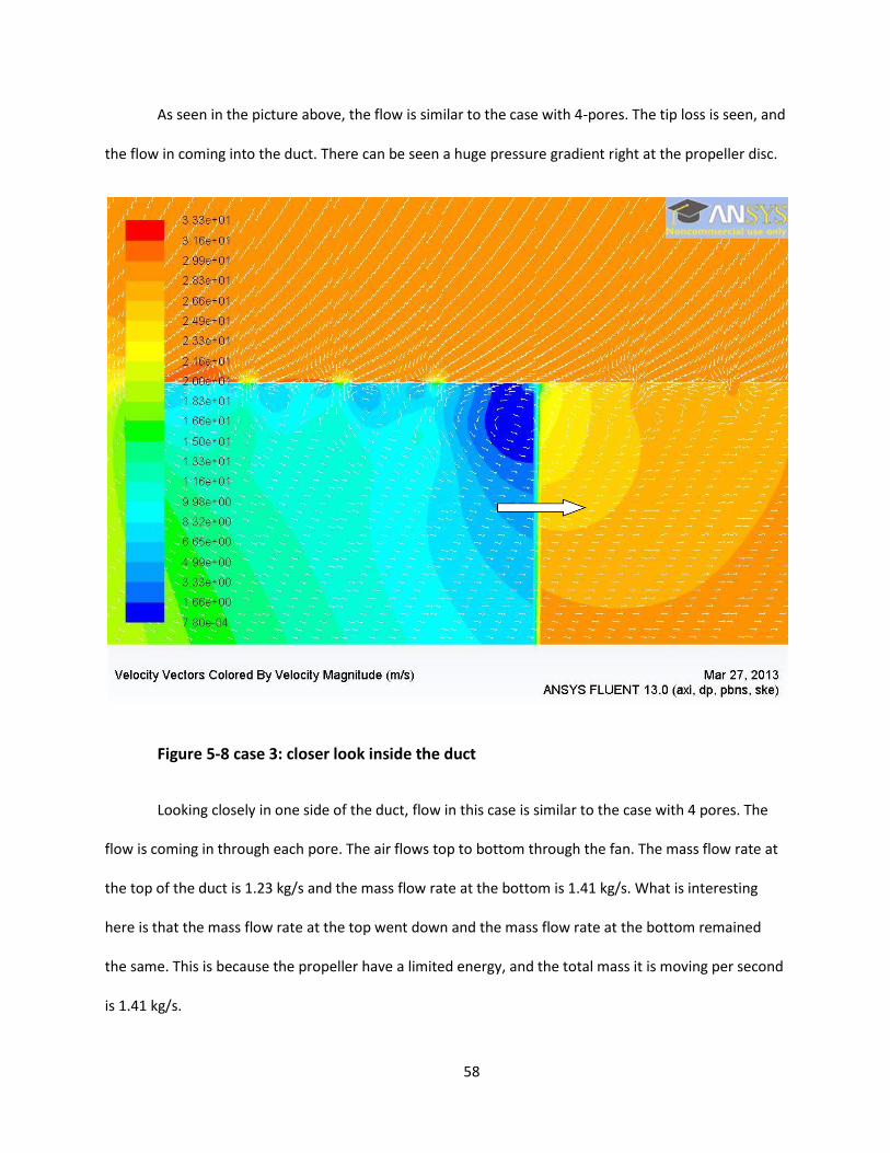
As seen in the picture above, the flow is similar to the case with 4-pores. The tip loss is seen, and

the flow in coming into the duct. There can be seen a huge pressure gradient right at the propeller disc.

Figure 5-8 case 3: closer look inside the duct

Looking closely in one side of the duct, flow in this case is similar to the case with 4 pores. The

flow is coming in through each pore. The air flows top to bottom through the fan. The mass flow rate at

the top of the duct is 1.23 kg/s and the mass flow rate at the bottom is 1.41 kg/s. What is interesting

here is that the mass flow rate at the top went down and the mass flow rate at the bottom remained

the same. This is because the propeller have a limited energy, and the total mass it is moving per second

is 1.41 kg/s.

59

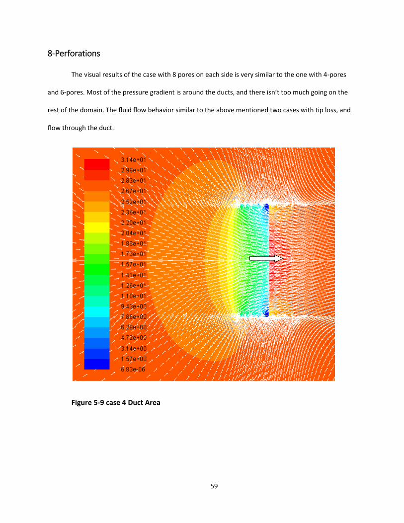
8-Perforations

The visual results of the case with 8 pores on each side is very similar to the one with 4-pores

and 6-pores. Most of the pressure gradient is around the ducts, and there isn’t too much going on the

rest of the domain. The fluid flow behavior similar to the above mentioned two cases with tip loss, and

flow through the duct.

Figure 5-9 case 4 Duct Area

60

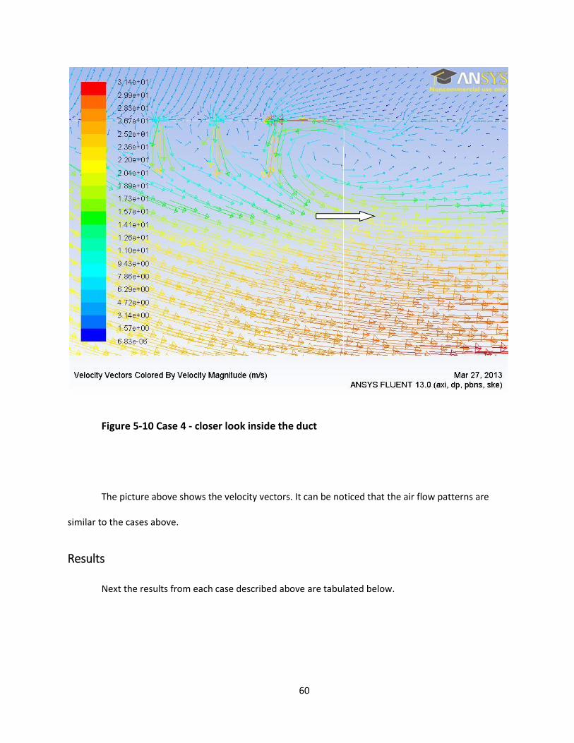
Figure 5-10 Case 4 - closer look inside the duct

The picture above shows the velocity vectors. It can be noticed that the air flow patterns are

similar to the cases above.

Results

Next the results from each case described above are tabulated below.

61

Table 5 : Results for 6000 Pa Pressure input

As it can be seen in table 5, the thrust was found to be increasing as perforations were added in the duct. The efficiency of the case with

no duct was found to be the highest. The maximum velocity was around 95m/s. That is a lot of speed of air. The speed of air increased with the

addition of duct.

Case

Open Area

of the duct

Pressure

input

Area for

calculating

thrust

Max

Velocity

Pressure

Force Mom. Flux

Pressure

Force Mom. Flux

Thrust

Produced

Duct

Weight Net Thrust Efficiency Ct

Pa m2 m/s N N N N N N N %

1 0% 6000 0.1110 95.4 -1.603 -307.604 -278.654 304.954 275.701 1.716 273.985 90% 0.223

2 8% 6000 0.1134 95.1 -4.106 -306.179 -216.997 242.166 276.905 1.579 275.326 91% 0.220

3 12% 6000 0.1075 94.4 -2.795 -305.276 -187.056 210.834 278.702 1.510 277.191 91% 0.237

4 16% 6000 0.1134 93.8 -0.873 -303.417 -164.231 186.463 280.313 1.442 278.871 92% 0.229

5 24% 6000 0.1134 93.8 0.649 -297.935 -142.073 157.902 282.756 1.304 281.451 93% 0.231

6 36% 6000 0.1110 93.2 4.283 -298.875 -99.750 121.448 283.500 1.098 282.402 93% 0.240

7 40% 6000 0.1110 93.2 3.761 -299.430 -94.691 112.381 285.500 1.030 284.470 94% 0.242

8 48% 6000 0.1110 93.1 6.674 -296.702 -76.117 96.084 286.409 0.892 285.517 94% 0.243

9 60% 6000 0.1110 93.2 7.984 -295.528 -62.912 78.218 288.206 0.687 287.519 95% 0.244

10 80% 6000 0.1075 93.5 12.903 -290.791 -44.157 57.197 290.654 0.343 290.311 95% 0.252

11 96% 6000 0.1134 92.9 16.509 -288.768 -36.440 53.721 287.996 0.069 287.927 95% 0.240

12 100% 6000 0.1257 88.5 31.188 -288.617 -46.613 71.385 297.610 0.000 297.610 98% 0.247

62

Table 6 Results for 3000 Pa pressure input

Similar effects can be observed in cases with 3000 Pa input pressure. The cases with no duct were found to be the most efficient and

created the most thrust. The maximum speed of the air was seen to increase with the addition of duct.

Case

Open Area Pressure

input

Area for

calculating

thrust

Max

Velocity

Pressure

Force Mom. Flux

Pressure

Force Mom. Flux

Thrust

Produced

Duct

Weight Net Thrust Efficiency Ct

Pa m2 m/s N N N N N N N %

1 0% 3000 0.0507 67.4 -0.323 -151.448 -133.344 146.679 137.790 1.716 136.074 90% 0.230

2 8% 3000 0.1075 67.2 -2.023 -152.970 -108.431 121.094 138.284 1.579 136.705 90% 0.232

3 12% 3000 0.1075 66.7 -1.405 -152.618 -93.639 105.515 139.337 1.510 137.826 91% 0.238

4 16% 3000 0.1075 66.3 -0.426 -151.684 -82.078 93.296 140.039 1.442 138.597 91% 0.235

5 24% 3000 0.1134 66.0 0.412 -150.534 -71.060 80.853 141.152 1.304 139.847 92% 0.233

6 36% 3000 0.1257 65.8 1.749 -149.304 -52.667 61.042 142.679 1.098 141.580 93% 0.234

7 40% 3000 0.1075 65.8 1.884 -149.699 -47.442 56.359 142.665 1.030 141.635 93% 0.250

8 48% 3000 0.1122 65.7 2.983 -148.254 -40.351 48.351 143.236 0.892 142.344 94% 0.241

9 60% 3000 0.1075 65.8 4.004 -147.751 -31.531 39.257 144.029 0.687 143.343 94% 0.253

10 80% 3000 0.1075 66.1 6.438 -145.371 -22.228 28.726 145.312 0.343 144.969 95% 0.253

12 100% 3000 0.1195 62.4 15.850 -144.276 -23.154 35.763 147.518 0.000 147.518 97% 0.259

Bottom Top

63

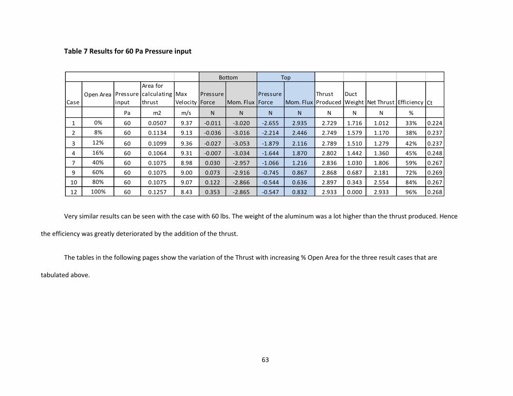
Table 7 Results for 60 Pa Pressure input

Very similar results can be seen with the case with 60 lbs. The weight of the aluminum was a lot higher than the thrust produced. Hence

the efficiency was greatly deteriorated by the addition of the thrust.

The tables in the following pages show the variation of the Thrust with increasing % Open Area for the three result cases that are

tabulated above.

CaseOpen Area Pressure

input

Area for

calculating

thrust

Max

Velocity

Pressure

Force Mom. Flux

Pressure

Force Mom. Flux

Thrust

Produced

Duct

Weight Net Thrust Efficiency Ct

Pa m2 m/s N N N N N N N %

1 0% 60 0.0507 9.37 -0.011 -3.020 -2.655 2.935 2.729 1.716 1.012 33% 0.224

2 8% 60 0.1134 9.13 -0.036 -3.016 -2.214 2.446 2.749 1.579 1.170 38% 0.237

3 12% 60 0.1099 9.36 -0.027 -3.053 -1.879 2.116 2.789 1.510 1.279 42% 0.237

4 16% 60 0.1064 9.31 -0.007 -3.034 -1.644 1.870 2.802 1.442 1.360 45% 0.248

7 40% 60 0.1075 8.98 0.030 -2.957 -1.066 1.216 2.836 1.030 1.806 59% 0.267

9 60% 60 0.1075 9.00 0.073 -2.916 -0.745 0.867 2.868 0.687 2.181 72% 0.269

10 80% 60 0.1075 9.07 0.122 -2.866 -0.544 0.636 2.897 0.343 2.554 84% 0.267

12 100% 60 0.1257 8.43 0.353 -2.865 -0.547 0.832 2.933 0.000 2.933 96% 0.268

Bottom Top

64

Figure 5-11 variation of net Thrust with % of open area in the duct for cases with 6000

Pa after duct weight is subtracted from the thrust

From the figure above, it can be seen that the thrust increases as the % of Open area is

increased. This is because as the amount of duct surface is decreased, the drag provided by the duct

decreases as well ultimately responsible decreasing the thrust. The total decrease in thrust by addition

of duct was about 22N. Addition of ducts produced 7% less thrust. When the duct weight was included,

from the image above, it can be seen that the thrust is lowered with the addition of duct.

270.000

275.000

280.000

285.000

290.000

295.000

300.000

0% 10% 20% 30% 40% 50% 60% 70% 80% 90% 100%

Thru

st [

N]

% of Open Area

Thrust vs % of Open Area (6000 Pa)

Thrust vs % of Open Area

Thrust including Duct weight

65

Figure 5-12 variation of net Thrust with % of Open Area for cases with 3000 Pa after

duct weight is subtracted from the thrust

From the cases with 3000 Pa Pressure Difference, it can be seen that the thrust increases as the

% of Open area is increased just like in the case with 6000 Pa. The loss in thrust is more when the duct

weight is included. The slope of the line decreases slightly after about 30% open area here too. The total

decrease in thrust by addition of duct was about 10N. The ducted propellers produce around 7% less

thrust than the free propellers.

134.000

136.000

138.000

140.000

142.000

144.000

146.000

148.000

150.000

0% 10% 20% 30% 40% 50% 60% 70% 80% 90% 100%

Thru

st [

N]

% of Open Area

Thrust vs. % Open Area- 3000 Pa

Thrust vs % of Open Area 3000 Pa

Thrust including Duct weight

66

Figure 5-13 Variation of net Thrust with % of Open Area for cases with 60 Pa after duct

weight is subtracted from the thrust

From the cases with 60 Pa Pressure Difference, it can be seen that the thrust increases as the %

of Open area is increased just like in the case with 6000 Pa and 3000 Pa., For this case, when duct weight

is included in the calculations, the difference in thrust is a lot more significant. The slope of the line

decreases slightly after about 20% open area here. The total decrease in thrust by addition of duct was

about 0.2 N. The ducted propellers produced around 7% less thrust than the free propellers.

0.000

0.500

1.000

1.500

2.000

2.500

3.000

3.500

0% 10% 20% 30% 40% 50% 60% 70% 80% 90% 100%

Thru

st

% Open Area

Thrust vs % Open Area for 60 Pa

Thrust vs % of Open Area 60 Pa

Thrust including Duct Weight

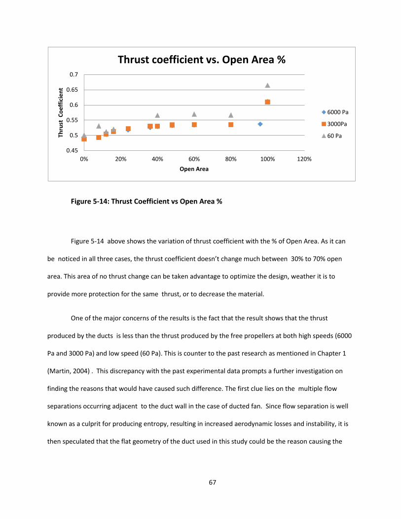
67

Figure 5-14: Thrust Coefficient vs Open Area %

Figure 5-14 above shows the variation of thrust coefficient with the % of Open Area. As it can

be noticed in all three cases, the thrust coefficient doesn’t change much between 30% to 70% open

area. This area of no thrust change can be taken advantage to optimize the design, weather it is to

provide more protection for the same thrust, or to decrease the material.

One of the major concerns of the results is the fact that the result shows that the thrust

produced by the ducts is less than the thrust produced by the free propellers at both high speeds (6000

Pa and 3000 Pa) and low speed (60 Pa). This is counter to the past research as mentioned in Chapter 1

(Martin, 2004) . This discrepancy with the past experimental data prompts a further investigation on

finding the reasons that would have caused such difference. The first clue lies on the multiple flow

separations occurring adjacent to the duct wall in the case of ducted fan. Since flow separation is well

known as a culprit for producing entropy, resulting in increased aerodynamic losses and instability, it is

then speculated that the flat geometry of the duct used in this study could be the reason causing the

0.45

0.5

0.55

0.6

0.65

0.7

0% 20% 40% 60% 80% 100% 120%

Thru

st C

oe

ffic

ien

t

Open Area

Thrust coefficient vs. Open Area %

6000 Pa

3000Pa

60 Pa

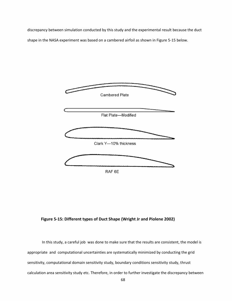
68

discrepancy between simulation conducted by this study and the experimental result because the duct

shape in the NASA experiment was based on a cambered airfoil as shown in Figure 5-15 below.

Figure 5-15: Different types of Duct Shape (Wright Jr and Piolene 2002)

In this study, a careful job was done to make sure that the results are consistent, the model is

appropriate and computational uncertainties are systematically minimized by conducting the grid

sensitivity, computational domain sensitivity study, boundary conditions sensitivity study, thrust

calculation area sensitivity study etc. Therefore, in order to further investigate the discrepancy between

69

this computational simulation with the expermental data, it is recommended that ducts with various

cambered airfoil configuration be conducted in future studies.

Conclusions:

A 2-D CFD simulation was conducted to investigate whether the hypothesis of adding

perforations to (or removing material from) the propeller duct can benefit from a net thrust gain in

comparison of no-duct free propellers. The conclusions are:

1. A computational mode was successfully developed and implemented by modeling the propeller

with a pressure jump across a actuate disc with an infinitesimal small thickness.

2. In contrast to the previous experimental results, adding duct to a free propeller does not

increase but reduces the thrust even when the weight is not considered.

3. Both gross and next thrusts increase as more perforations are added on the ducts. More net

thrust is gained as more perforations are added (i.e. more duct weight is reduced) until the

maximum thrust is achieved for the no-duct free propeller.

4. More gross thrust is gained with more perforations could be explained with the fact that small

jets produced by the perforations actually reduce the adverse effect of multiple flow

separations.

5. The dimensionless thrust remains almost constant between 40%-80% perforations. This region

can be conveniently used during design of ducted propellers.

6. The discrepancy between the present simulation results and the previous experimental results

is suspected being caused by not having the cambered airfoil duct wall configuration because

NASA's experiments used cambered airfoil duct wall while the flat-wall configuration used in

this study has generated multiple flow separation. Further study is recommended to continue

70

more detailed computational simulation using a duct with cambered airfoil configuration to

reduce the aerodynamic losses.

71

BIBLIOGRAPHY

2011. A robot that flies like a bird. http://www.ted.com/talks/a_robot_that_flies_like_a_bird.html.

Airforce, Wright Patterson. 2012. AirForce Research Laboratory. http://www.wpafb.af.mil/afrl/.

Ansys. 2013. "Ansys Help - Theory Manual." Ansys.

Boyle, Rebecca. 2012. PopSci. http://www.popsci.com/technology/article/2012-04/video-flying-shape-

thing-propels-itself-flipping-inside-out.

Dixon, S.L, and C.A Hall. 2010. Fluid Mechanics and Thermodynamics of Turbomachinery. 6th.

Butterworth-Heinemann .

Festo. 2012. smart bird - bird flight deciphered. http://www.festo.com/cms/en_corp/11369.htm.

Forman, Erick. 2012. Eric Forman Blog. April 25. http://www.ericforman.com/blog/smart-inversion-

flying-inflatable-shape-by-festo/.

Galante, Nick. 2001. Helios Prototype. NASA. July 14.

http://www.dfrc.nasa.gov/Gallery/Photo/Helios/Large/ED01-0209-3.jpg.

HobbyKing. 2013. 02 10.

http://www.hobbyking.com/hobbyking/store/__18120__Turnigy_Aerodrive_SK3_3542_1185kv

_Brushless_Outrunner_Motor.html.

James, Gregory K. 2000. "Unmanned aerial vehicles and special operations: Future direction." Masters

Thesis, Aeronautics and astronautivs, University of Washington.

Joblin, Steve. 2100. RCGroups. Jan 16.

http://www.rcgroups.com/forums/showthread.php?t=1335765&page=21.

72

Martin, Preston, and Chee Tung. 2004. Performance and Flowfield Measurements on a 10-inch Ducted

Rotor VTOL UAV. California: Ames Research Center, Moffett Field.

Martin, Preston, and Chee Tung. 2004. Performance and Flowfield Measurements on a 10-inch Ducted

Rotor VTOL UAV. pdf document. Ca: NASA Rotorcraft Division.

MIT. 1997. "Theory of Flight." web.mit.edu. March 16. http://web.mit.edu/16.00/www/aec/flight.html.

Munson, Bruce R, Donald F Young, and Theodore H Okiishi. 2008. Fundamentals of FLuid Mechanics. 3e.

New York: John Wiley & Sons. Inc. Accessed 01 2013.

NASA. n.d. Nasa.gov. http://www.nasa.gov/centers/dryden/news/FactSheets/FS-034-DFRC.html.

Nick, Carlos, Gabe, Chris. 2013. kickstarter.com. 1.

http://www.kickstarter.com/projects/1671680066/incredible-hlq-heavy-lift-quadcopter.

n.d. Open Course Ware MIT - Unified Propulsion. Accessed 12 15, 2012.

http://ocw.mit.edu/ans7870/16/16.unified/propulsionS04/UnifiedPropulsion9/UnifiedPropulsio

n9.htm.

Piasecki Aircraft Corporation. 2009. X-49A SpeedHawk. http://www.piasecki.com/x49a.php.

Scott, Jeff. 2001. AeroSpaceweb.org. July 29.

http://www.aerospaceweb.org/question/aerodynamics/q0037.shtml.

Seddon, John, and Simon Newman. 2011. Basic Helicopter Aerodynamivs. John Wiley & Sons Ltd.

Solon, Olivia. 2013. Wired.com. 03. http://www.wired.co.uk/news/archive/2013-03/27/iranian-rescue-

robot.

73

The Muslim Observer. 2010. The Next Step: A Stealth Drone. Washington, Jan 4.

http://muslimmedianetwork.com/mmn/?tag=us-air-force.

Trimble, Stephen. 2009. Flightglobal - aviation connected. May 6.

http://www.flightglobal.com/news/articles/socom-reveals-plan-to-buy-20-improved-and-

renamed-a160t-hummingbirds-326071/.

Tzafestas, S.G. 2007. "Advances in Unmanned Aerial Vehicle." Intelligent Systems, controls, and

automation: Science and Engineering.

Wright Jr, George E., and E. Marc de Piolene. 2002. Ducted Fan Design. Millenial year Ed. Mass Flow.

74

Chapter 6 : APPENDICES

Appendix I: Different Cases

The images of different cases is shown in the figures below.

75

Figure 6-1 Duct with no Pores Figure 6-2: Duct with four 0.1"

Pores

Figure 6-3 Duct with six 0.1"

Diameter Pores

Figure 6-4 Eight 0.1"

Diameter Pores

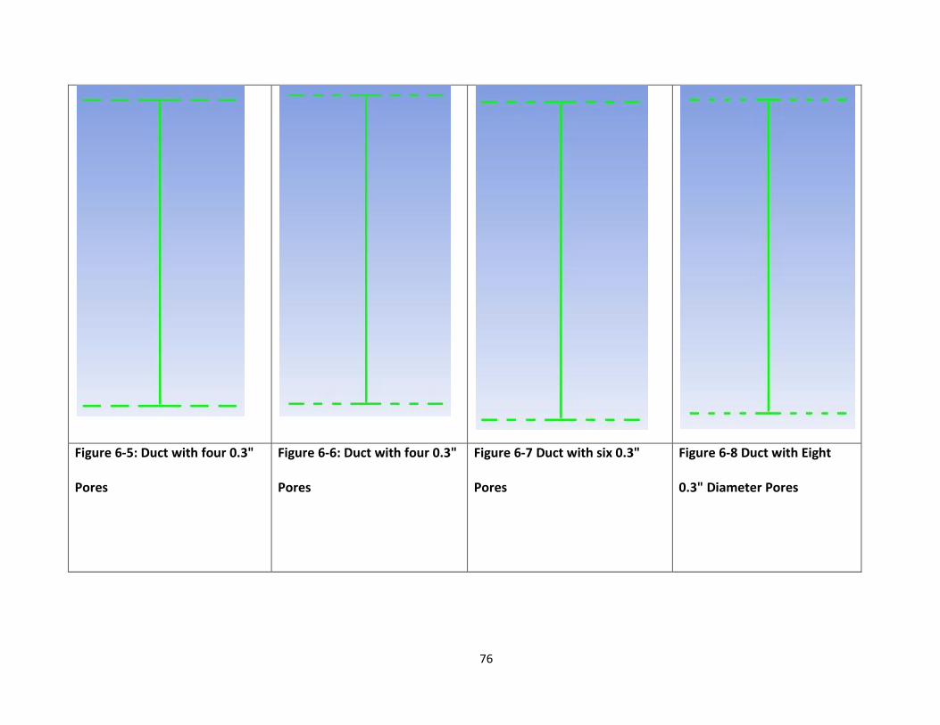
76

Figure 6-5: Duct with four 0.3"

Pores

Figure 6-6: Duct with four 0.3"

Pores

Figure 6-7 Duct with six 0.3"

Pores

Figure 6-8 Duct with Eight

0.3" Diameter Pores

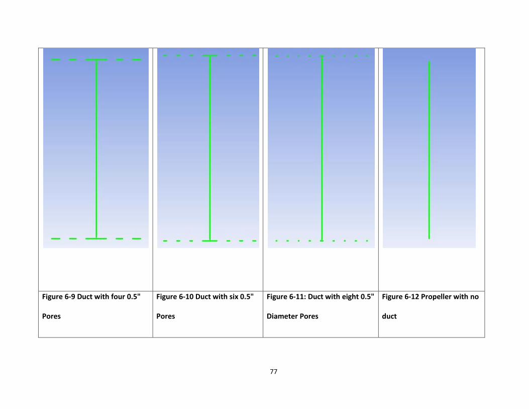
77

Figure 6-9 Duct with four 0.5"

Pores

Figure 6-10 Duct with six 0.5"

Pores

Figure 6-11: Duct with eight 0.5"

Diameter Pores

Figure 6-12 Propeller with no

duct

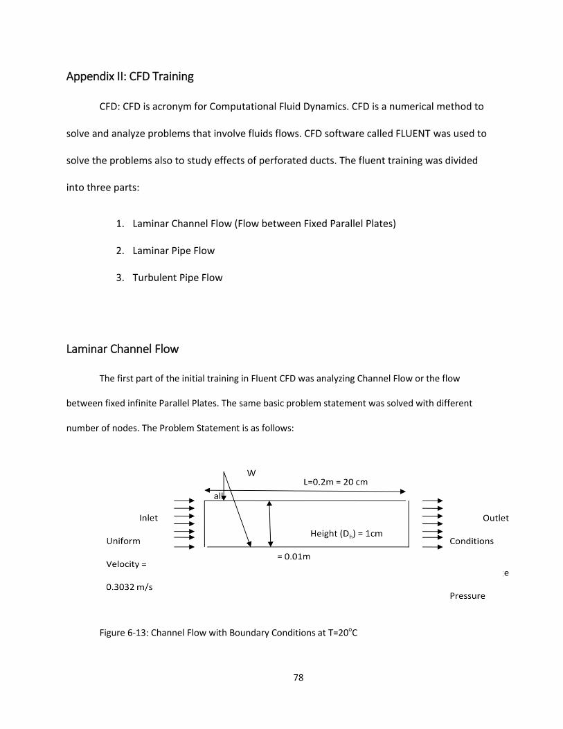
78

Appendix II: CFD Training

CFD: CFD is acronym for Computational Fluid Dynamics. CFD is a numerical method to

solve and analyze problems that involve fluids flows. CFD software called FLUENT was used to

solve the problems also to study effects of perforated ducts. The fluent training was divided

into three parts:

1. Laminar Channel Flow (Flow between Fixed Parallel Plates)

2. Laminar Pipe Flow

3. Turbulent Pipe Flow

Laminar Channel Flow

The first part of the initial training in Fluent CFD was analyzing Channel Flow or the flow

between fixed infinite Parallel Plates. The same basic problem statement was solved with different

number of nodes. The Problem Statement is as follows:

Figure 6-13: Channel Flow with Boundary Conditions at T=20oC

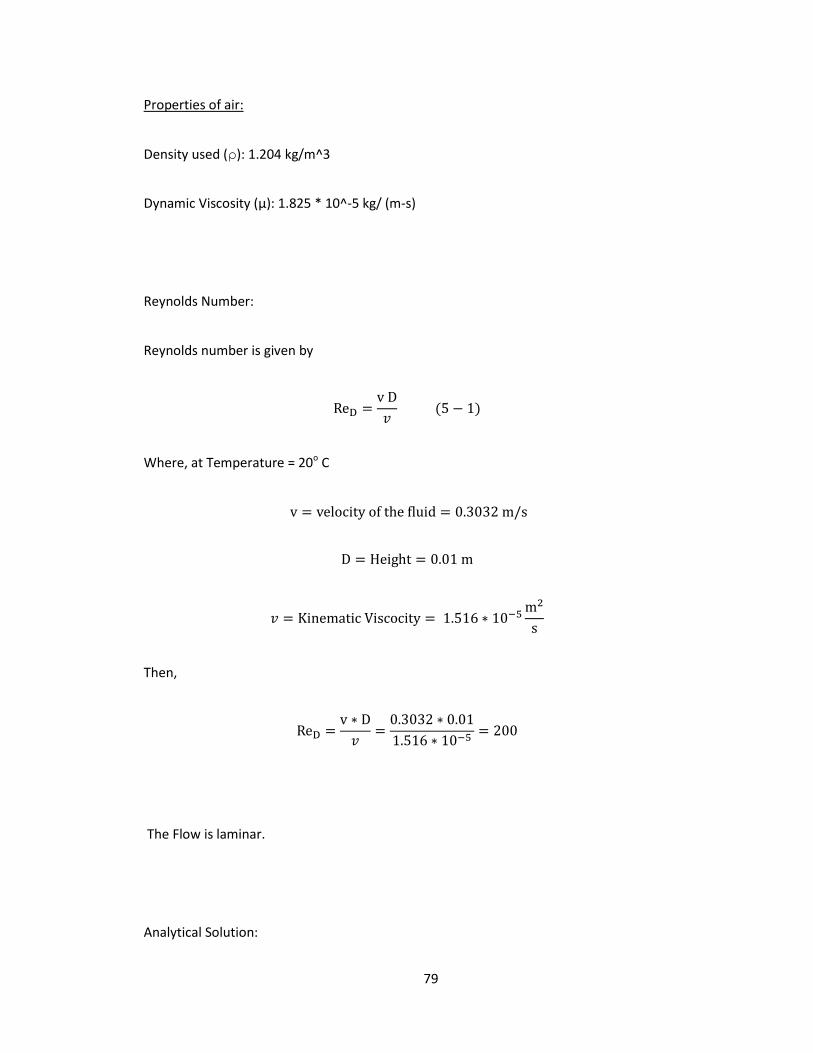
79

Properties of air:

Density used (ρ): 1.204 kg/m^3

Dynamic Viscosity (µ): 1.825 * 10^-5 kg/ (m-s)

Reynolds Number:

Reynolds number is given by

Where, at Temperature = 20o C

Then,

The Flow is laminar.

Analytical Solution:

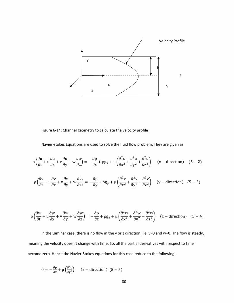
80

Figure 6-14: Channel geometry to calculate the velocity profile

Navier-stokes Equations are used to solve the fluid flow problem. They are given as:

In the Laminar case, there is no flow in the y or z direction, i.e. v=0 and w=0. The flow is steady,

meaning the velocity doesn’t change with time. So, all the partial derivatives with respect to time

become zero. Hence the Navier-Stokes equations for this case reduce to the following:

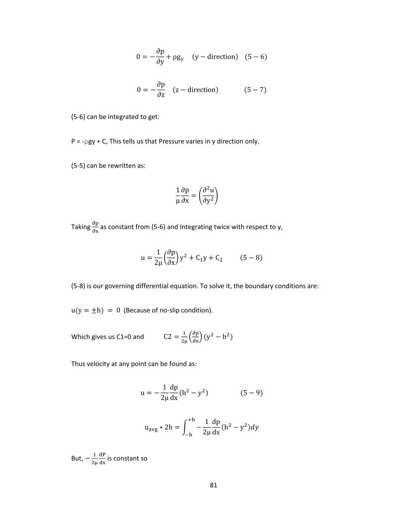
81

(5-6) can be integrated to get:

P = -ρgy + C, This tells us that Pressure varies in y direction only.

(5-5) can be rewritten as:

Taking

as constant from (5-6) and Integrating twice with respect to y,

(5-8) is our governing differential equation. To solve it, the boundary conditions are:

(Because of no-slip condition).

Which gives us C1=0 and

Thus velocity at any point can be found as:

But,

is constant so

82

This velocity is compared to the profile obtained from Fluent to verify Fluent’s solution.

Equations used by Fluent:

The Continuity equation is given by:

The momentum conservation equation is given by:

Where,

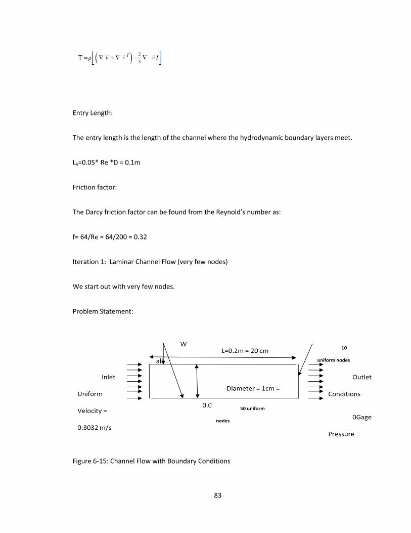
83

Entry Length:

The entry length is the length of the channel where the hydrodynamic boundary layers meet.

Lh=0.05* Re *D = 0.1m

Friction factor:

The Darcy friction factor can be found from the Reynold’s number as:

f= 64/Re = 64/200 = 0.32

Iteration 1: Laminar Channel Flow (very few nodes)

We start out with very few nodes.

Problem Statement:

Figure 6-15: Channel Flow with Boundary Conditions

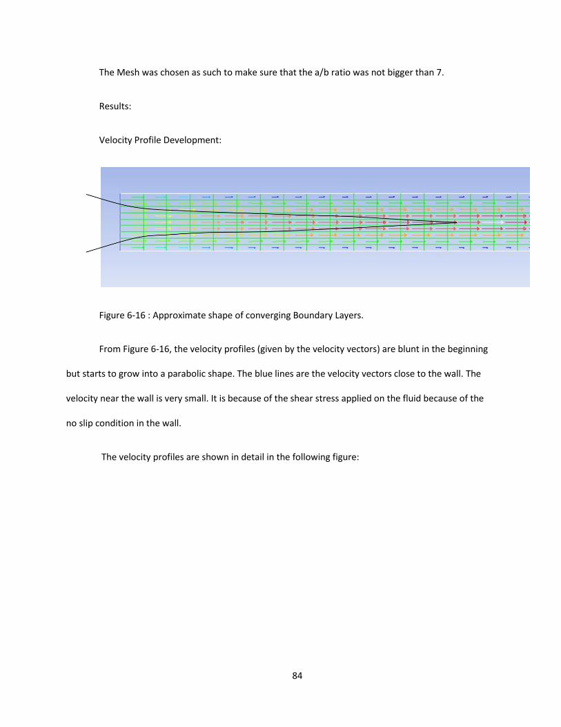
84

The Mesh was chosen as such to make sure that the a/b ratio was not bigger than 7.

Results:

Velocity Profile Development:

Figure 6-16 : Approximate shape of converging Boundary Layers.

From Figure 6-16, the velocity profiles (given by the velocity vectors) are blunt in the beginning

but starts to grow into a parabolic shape. The blue lines are the velocity vectors close to the wall. The

velocity near the wall is very small. It is because of the shear stress applied on the fluid because of the

no slip condition in the wall.

The velocity profiles are shown in detail in the following figure:

85

Figure 6-17 :The velocity Profile develops into parabolic velocity profile.

In the figure above, at inlet, the velocity is uniform. As it moves further inside the channel, the

profile starts taking the shape of a parabola. The velocity in the center line is the maximum while

velocity close to the wall is the smallest. This velocity profile at x=0.1 can be compared with the

expected velocity profile to check its accuracy.

0

0.002

0.004

0.006

0.008

0.01

0.012

0 0.1 0.2 0.3 0.4 0.5

Y-c

oo

rdin

ate

(m

)

x-velocity (m/s)

Ideal velocity profile vs Fluent's velocity profile

Ideal velocity Profile

Fluent's velocity Profile

86

Figure 6-18: Comparison of Ideal velocity profile vs. the velocity profile from Fluent

The Max error in the velocity profile is 3.528%. Since this system has no convective acceleration,

exact solution from Navier-Stokes equations is expected.

Next looking at the skin friction coefficient at the walls, the skin friction coefficient decreases all

the way to zero; this is not what one would expect.

Figure 6-19 : Skin friction-coefficient

The mesh is coarse, and there are no nodes in the center of the channel, because of which the

maximum velocity is not fully represented in this iteration. Hence A second iteration is done with more

nodes to see if number of nodes matters. The comparative study will be presented at the end.

Iteration 2: Increased Mesh Density

In this iteration the number of nodes is bumped to check if the solution gets better:

Problem Statement:

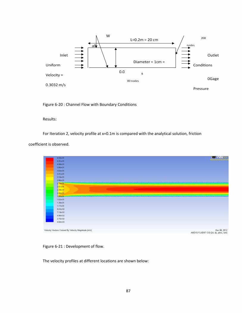
87

Figure 6-20 : Channel Flow with Boundary Conditions

Results:

For Iteration 2, velocity profile at x=0.1m is compared with the analytical solution, friction

coefficient is observed.

Figure 6-21 : Development of flow.

The velocity profiles at different locations are shown below:

88

Figure 6-22 : Velocity profiles at different locations for a channel flow

In the picture above, the velocity profile starts developing right at the entrance of the pipe, and

develops into a fully developed flow. The solution is as expected Uavg = 2/3 * umax =2/3*0.45 = 0.3 m/s.

The velocity profile at x=0.1m is compared to an ideal profile of a fully developed flow. The Max error %

in this case is 1.53%. The max %error decreased from 3.528% to 1.53% with the increase in mesh

density.

0

0.002

0.004

0.006

0.008

0.01

0.012

0 0.1 0.2 0.3 0.4 0.5

He

igh

t o

f C

han

ne

l (m

)

x-velocity (m/s)

x-velocity vs y-coordinate

Ideal

FLuent

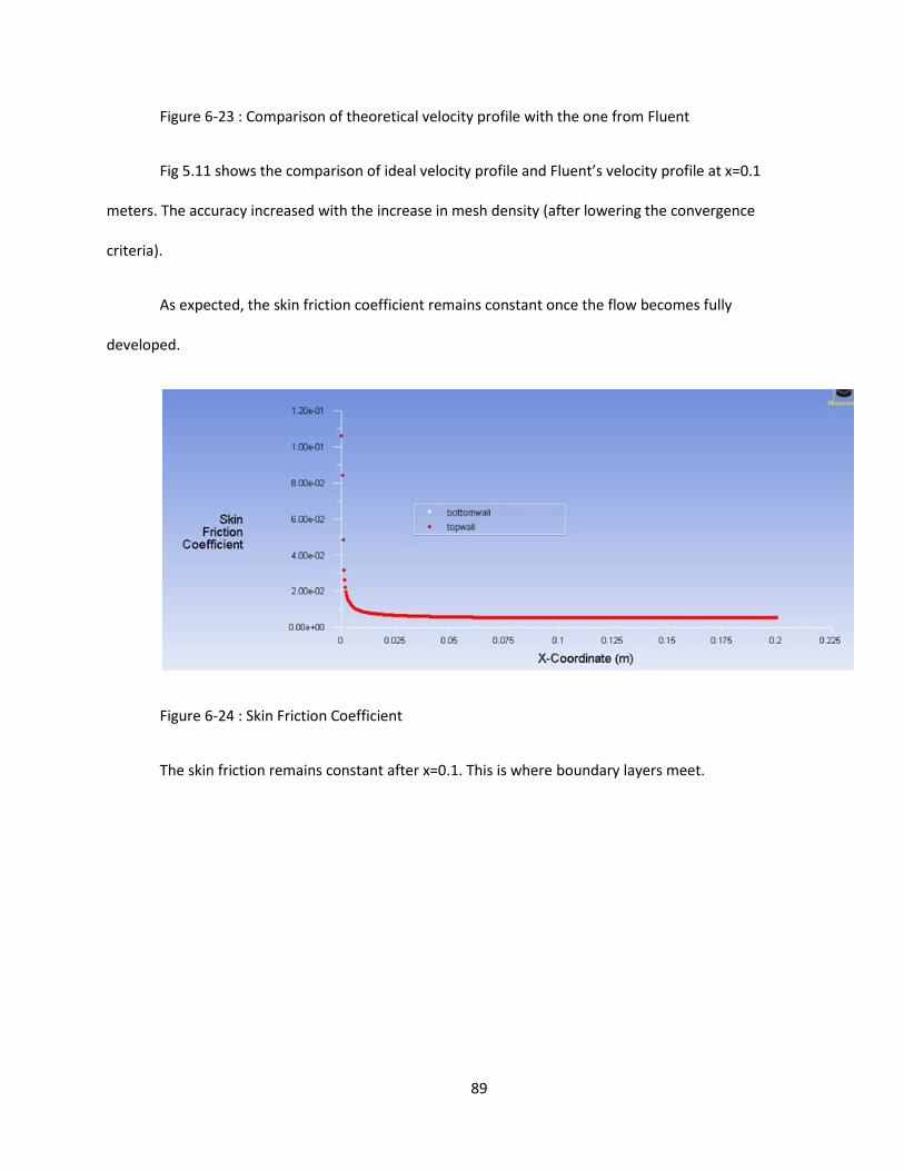
89

Figure 6-23 : Comparison of theoretical velocity profile with the one from Fluent

Fig 5.11 shows the comparison of ideal velocity profile and Fluent’s velocity profile at x=0.1

meters. The accuracy increased with the increase in mesh density (after lowering the convergence

criteria).

As expected, the skin friction coefficient remains constant once the flow becomes fully

developed.

Figure 6-24 : Skin Friction Coefficient

The skin friction remains constant after x=0.1. This is where boundary layers meet.

90

Figure 6-25 : A close look at the skin friction coefficient.

Skin Friction coefficient is a non-dimensional parameter defined as the ratio of wall shear stress

and the reference dynamic pressure

w/(1/2 ρref (Vref)2

A higher skin friction coefficient is usually expected for low Reynold’s number because the

viscous forces are still prominent as compared to the inertial forces. However our mesh is not dense

enough at the region close to the wall to fully capture the skin friction.

Iteration 3: Iteration 2 with increased convergence criteria

The absolute convergence criteria was increased to 10-8 and ran the analysis in fluent. The error

of 1.49% was seen which is a small improvement from the previous Iteration with the convergence

criteria of 10-6.

0.2, 0.0581784

0.04

0.045

0.05

0.055

0.06

0.065

0.07

0.075

0.08

0 0.05 0.1 0.15 0.2 0.25

Skin

Fri

ctio

n C

oe

ffic

ien

t

X-coordinate (m)

Skin Friction Coefficient

Skin Friction Coefficient

91

Figure 6-26 : Comparison with Ideal case for velocity profile

Fig: Comparing velocity profiles from fluent with the Ideal profiles, with refined mesh and very

small convergence criteria for momentum and velocity.

A closer look at the skin friction coefficient at this point gives us the following results:

0

0.002

0.004

0.006

0.008

0.01

0.012

0 0.1 0.2 0.3 0.4 0.5

Y-c

oo

rdin

ate

(m

)

x-velocity (m/s)

With convergence criteria 10^-8

Ideal

Fluent

0.2, 0.0578324

0.05

0.055

0.06

0.065

0.07

0.075

0.08

0.085

0.09

0.095

0.1

0 0.05 0.1 0.15 0.2 0.25

Skin

Fri

ctio

n C

oe

ffic

ien

t

Distance from the inlet (m)

Skin Friction Coefficient

Skin Friction Coefficient

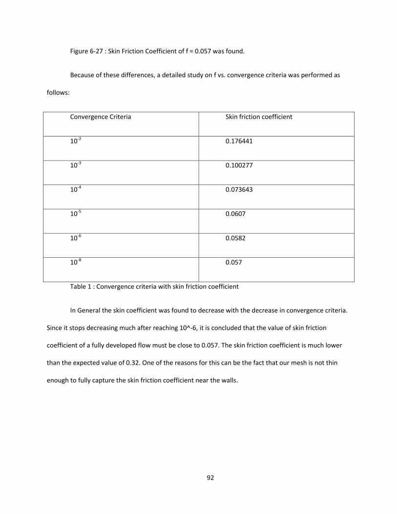
92

Figure 6-27 : Skin Friction Coefficient of f = 0.057 was found.

Because of these differences, a detailed study on f vs. convergence criteria was performed as

follows:

Convergence Criteria Skin friction coefficient

10-2 0.176441

10-3 0.100277

10-4 0.073643

10-5 0.0607

10-6 0.0582

10-8 0.057

Table 1 : Convergence criteria with skin friction coefficient

In General the skin coefficient was found to decrease with the decrease in convergence criteria.

Since it stops decreasing much after reaching 10^-6, it is concluded that the value of skin friction

coefficient of a fully developed flow must be close to 0.057. The skin friction coefficient is much lower

than the expected value of 0.32. One of the reasons for this can be the fact that our mesh is not thin

enough to fully capture the skin friction coefficient near the walls.

93

2.1: Steady, Laminar Flow in Circular Tubes and no Heat source.

Stead and laminar flow through circular tubes are commonly known as Poiuseuille Flow. They

are one of the most commonly studied flows by undergraduates. Fluent is used to solve the laminar pipe

flow in circular tubes, and is compared with analytical solutions found by solving Navier-Stokes

equations.

Problem Statement:

Figure 6-28 : Channel Flow with Boundary Conditions

The inlet condition is uniform velocity of 1 m/s which corresponds to the Reynolds’s number of

200 for a fluid with the below mention properties. There is no temperature change throughout the

system; hence the energy equation is turned off. In solving laminar flow, fluent uses two distinct

equations to solve for energy and momentum. The energy equation is turned off. The outlet condition is

0 gage pressure, so the pipe is exiting outside. The lower edge is made the axis and upper edge is made

the wall.

Reynolds Number:

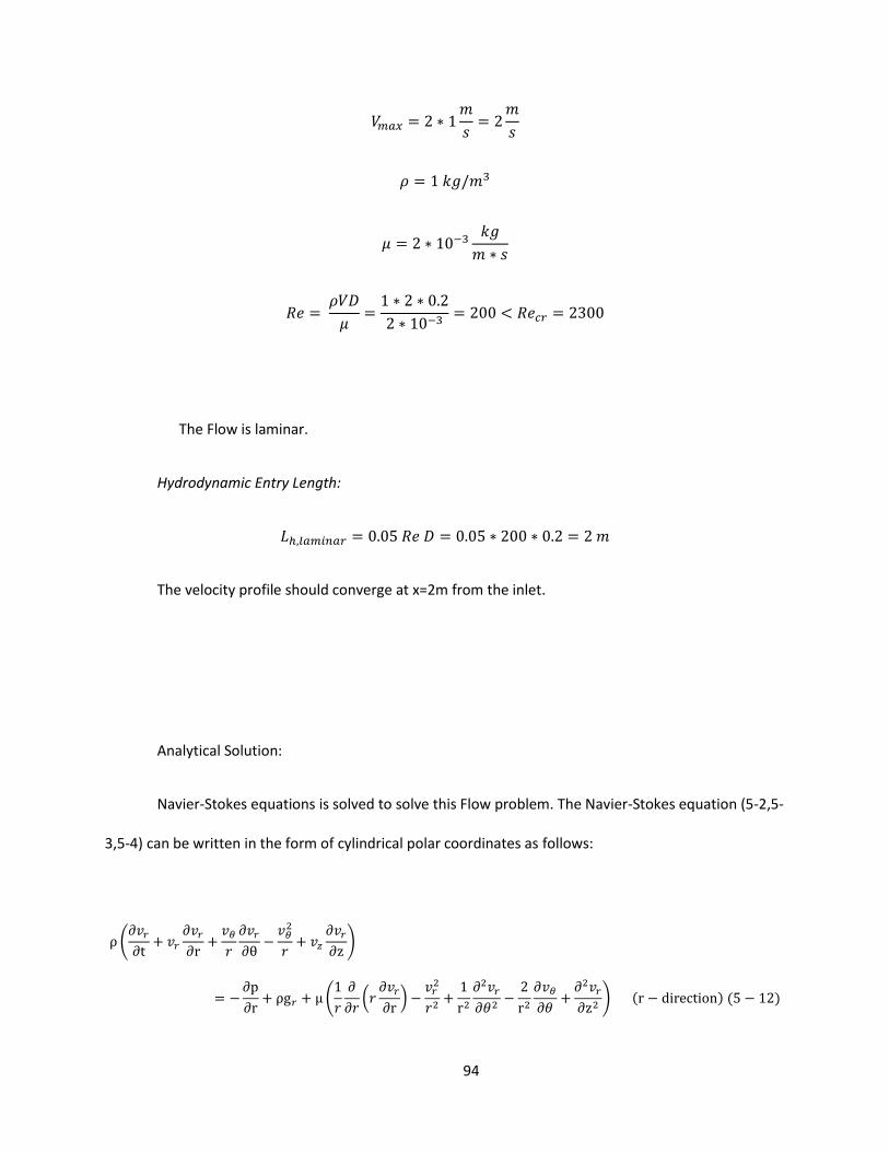
94

The Flow is laminar.

Hydrodynamic Entry Length:

The velocity profile should converge at x=2m from the inlet.

Analytical Solution:

Navier-Stokes equations is solved to solve this Flow problem. The Navier-Stokes equation (5-2,5-

3,5-4) can be written in the form of cylindrical polar coordinates as follows:

95

Assuming that the direction of the flow is perpendicular to the inlet, i.e. in z direction, steady

axisymmetric flow, the Navier-Stokes equation reduces to the following:

Integrating and solving the differential equations with the boundary conditions (wall velocity 0,

and finite velocity in the center), the following equation is obtained for velocity distribution.

Thus the velocity distribution of a fully developed flow is parabolic. Further integration and

simplification just like the one in the case of Laminar flow results in the following equation for maximum

velocity.

96

The velocity Profile of a fully developed laminar flow is given by

This velocity profile is compared to the profile obtained from Fluent to verify Fluent’s solution.

Equations used by Fluent:

For 2-D axisymmetric flow, the continuity equation is given by:

The momentum conservation is given by:

And

Pipe Flow Iteration 1:

97

For a pipe flow problem, a very simplified problem is solved to verify our method.

Meshing:

The Mesh was created using ICEM CFD. It has 5 elements in the vertical lines and 100 elements

in the horizontal lines. Total elements = 500. A coarse mesh was chosen on purpose to do a grid

sensitivity study.

Results:

The solution was converged in 48 time steps. The convergence criteria was 10^-6 for

momentum and velocity. The axial velocity vs. the Y-coordinate looks as in the picture below. The Vmax is

about 1.92 m/s. It is expected to be 2m/s.

Figure 6-29 : Solution with only 500 elements

Iteration: 2 (Refined Mesh with the same boundary conditions and physical properties)

In this iteration, the mesh is refined, and the solution is compared with the coarse mesh’s

results.

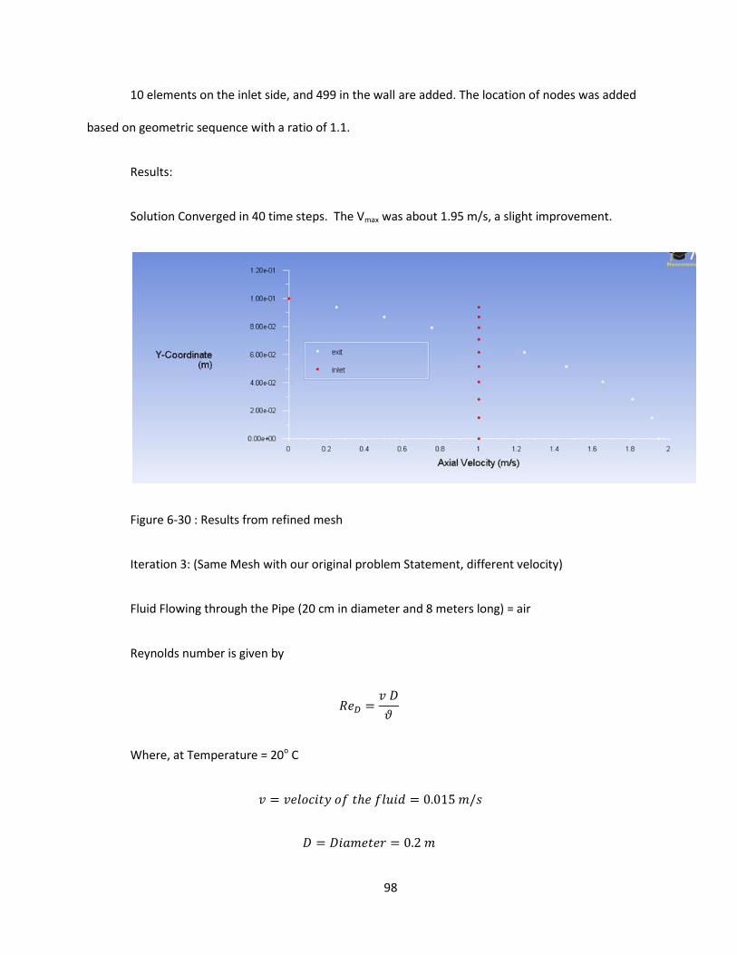
98

10 elements on the inlet side, and 499 in the wall are added. The location of nodes was added

based on geometric sequence with a ratio of 1.1.

Results:

Solution Converged in 40 time steps. The Vmax was about 1.95 m/s, a slight improvement.

Figure 6-30 : Results from refined mesh

Iteration 3: (Same Mesh with our original problem Statement, different velocity)

Fluid Flowing through the Pipe (20 cm in diameter and 8 meters long) = air

Reynolds number is given by

Where, at Temperature = 20o C

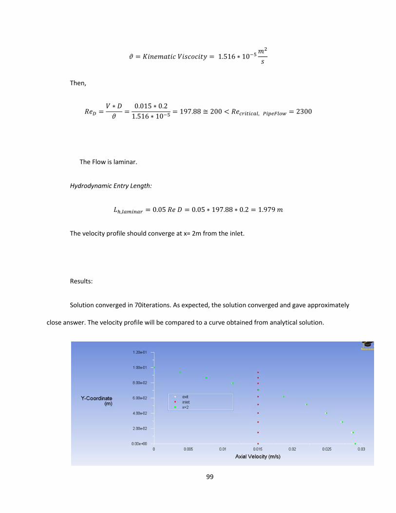
99

Then,

The Flow is laminar.

Hydrodynamic Entry Length:

The velocity profile should converge at x= 2m from the inlet.

Results:

Solution converged in 70iterations. As expected, the solution converged and gave approximately

close answer. The velocity profile will be compared to a curve obtained from analytical solution.

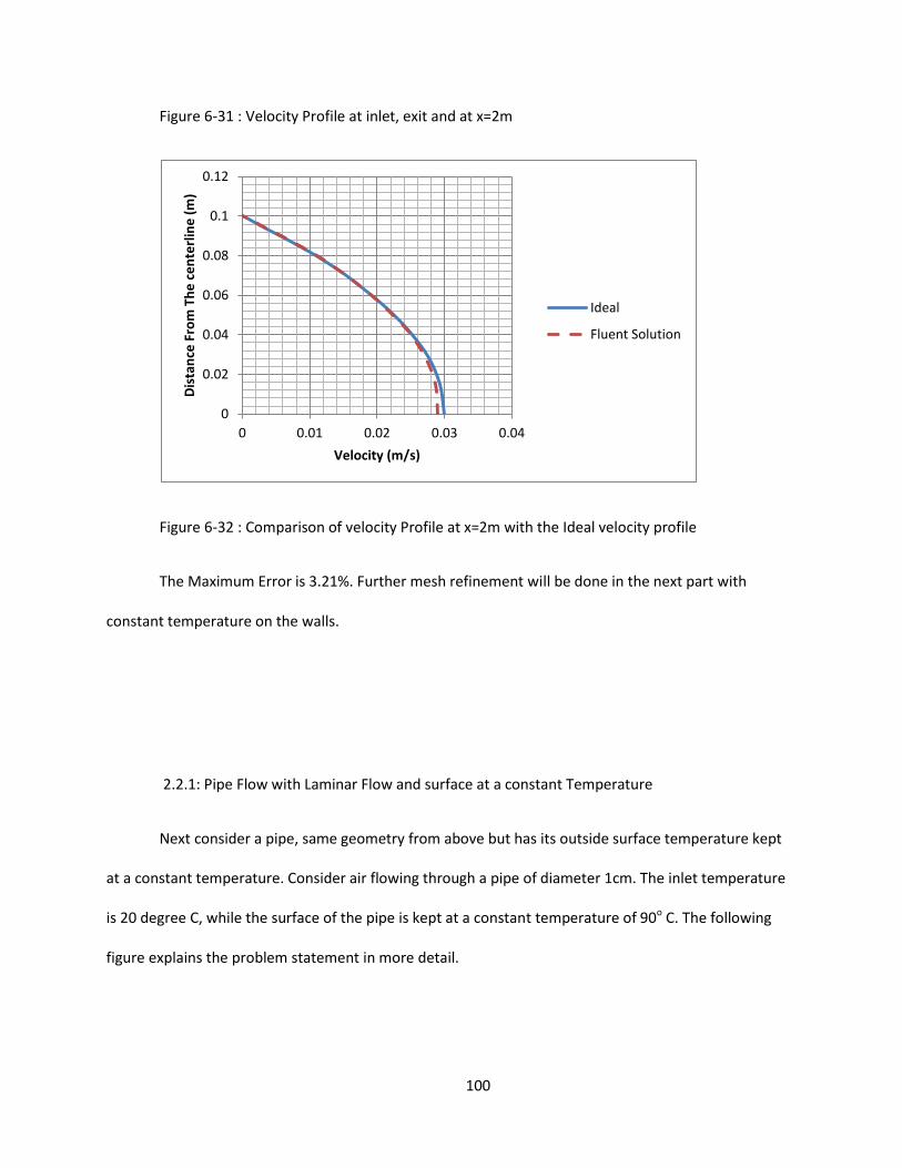
100

Figure 6-31 : Velocity Profile at inlet, exit and at x=2m

Figure 6-32 : Comparison of velocity Profile at x=2m with the Ideal velocity profile

The Maximum Error is 3.21%. Further mesh refinement will be done in the next part with

constant temperature on the walls.

2.2.1: Pipe Flow with Laminar Flow and surface at a constant Temperature

Next consider a pipe, same geometry from above but has its outside surface temperature kept

at a constant temperature. Consider air flowing through a pipe of diameter 1cm. The inlet temperature

is 20 degree C, while the surface of the pipe is kept at a constant temperature of 90o C. The following

figure explains the problem statement in more detail.

0

0.02

0.04

0.06

0.08

0.1

0.12

0 0.01 0.02 0.03 0.04

Dis

tan

ce F

rom

Th

e c

en

terl

ine

(m

)

Velocity (m/s)

Ideal

Fluent Solution

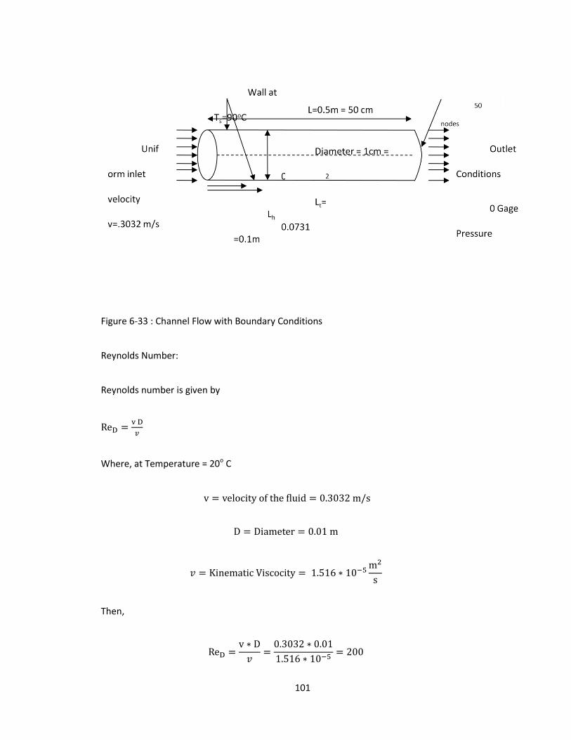
101

Figure 6-33 : Channel Flow with Boundary Conditions

Reynolds Number:

Reynolds number is given by

Where, at Temperature = 20o C

Then,

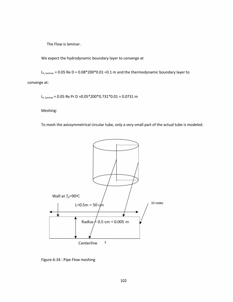
102

The Flow is laminar.

We expect the hydrodynamic boundary layer to converge at

Lh, laminar = 0.05 Re D = 0.08*200*0.01 =0.1 m and the thermodynamic boundary layer to

converge at:

Lt, laminar = 0.05 Re Pr D =0.05*200*0.731*0.01 = 0.0731 m

Meshing:

To mesh the axissymmetrical circular tube, only a very small part of the actual tube is modeled.

Figure 6-34 : Pipe Flow meshing

103

The mesh was created in CFD-ICEM. It had 10 nodes in the inlet/exit side and 130 nodes in the

centerline/ top wall. The solution converged in 30 steps.

Solutions comparison:

Hydrodynamic entry length and velocity profile

The velocity profile of a fully developed flow is given by the equation

Comparing the ideal velocity profile with the velocity profile at Lt the following curve is obtained:

Figure 6-35 : Comparison of Ideal vs. Fluent’s velocity Profile

Maximum error was 3.002 %.

0

0.001

0.002

0.003

0.004

0.005

0.006

0 0.2 0.4 0.6 0.8

Rad

ial C

oo

rdin

ate

(m

)

Axial velocity (m/s)

Ideal profile vs Fluent Profile

Ideal

Fluent Solution

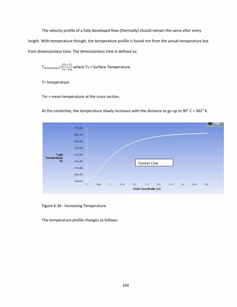
104

The velocity profile of a fully developed flow (thermally) should remain the same after entry

length. With temperature though, the temperature profile is found not from the actual temperature but

from dimensionless time. The dimensionless time is defined as:

Tdimensionless=

where Ts = Surface Temperature,

T= temperature

Tm = mean temperature at the cross section.

At the centerline, the temperature slowly increases with the distance to go up to 90o C = 362o K.

Figure 6-36 : Increasing Temperature

The temperature profile changes as follows:

Center Line

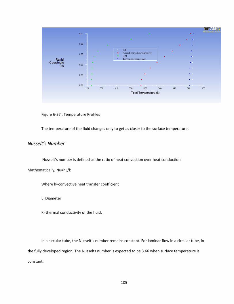
105

Figure 6-37 : Temperature Profiles

The temperature of the fluid changes only to get as closer to the surface temperature.

Nusselt’s Number

Nusselt’s number is defined as the ratio of heat convection over heat conduction.

Mathematically, Nu=hL/k

Where h=convective heat transfer coefficient

L=Diameter

K=thermal conductivity of the fluid.

In a circular tube, the Nusselt’s number remains constant. For laminar flow in a circular tube, in

the fully developed region, The Nusselts number is expected to be 3.66 when surface temperature is

constant.

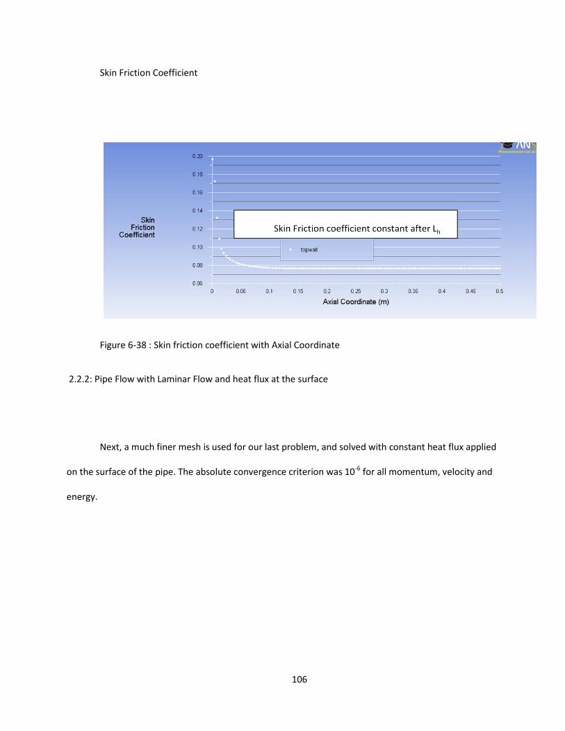
106

Skin Friction Coefficient

Figure 6-38 : Skin friction coefficient with Axial Coordinate

2.2.2: Pipe Flow with Laminar Flow and heat flux at the surface

Next, a much finer mesh is used for our last problem, and solved with constant heat flux applied

on the surface of the pipe. The absolute convergence criterion was 10-6 for all momentum, velocity and

energy.

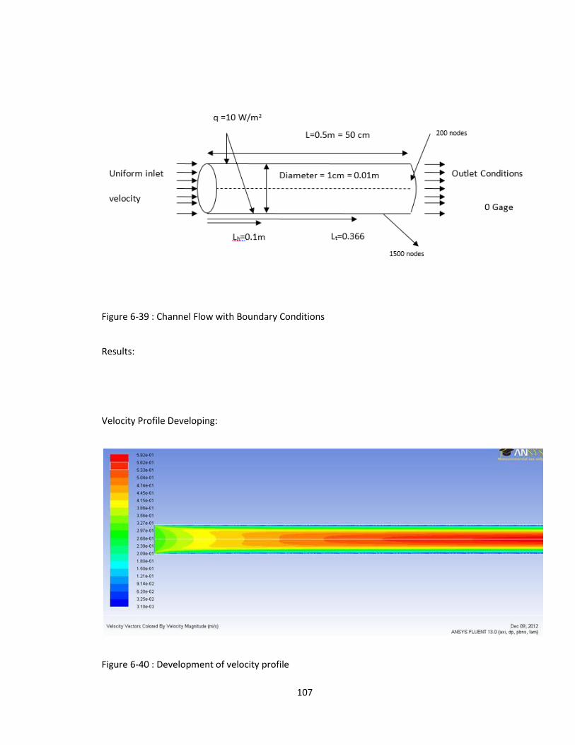
107

Figure 6-39 : Channel Flow with Boundary Conditions

Results:

Velocity Profile Developing:

Figure 6-40 : Development of velocity profile

108

Comparison of Ideal velocity profile with the Fluent Solution

Figure 6-41 : Comparison of ideal vs. Fluent’s velocity profile.

The max error % was 2.4%Skin Friction Coefficient

Figure 6-42 : Skin Friction Coefficient of 0.0392

Thermal Profile Developing:

0

0.002

0.004

0.006

0.008

0.01

0.012

0 0.2 0.4 0.6 0.8

r (m

)

Velocity (m/s)

Ideal velocity vs. Fluent's velocity Profile

Ideal velocity Profile

Fluent Velocity Profile

0

0.2

0.4

0.6

0.8

1

1.2

0 0.2 0.4 0.6

Skin

Fri

ctio

n C

oe

ffic

ien

t

X-Coordinate (m)

SkinFrictionCoefficient vs X-Coordinate (f=0.039244)

SkinFrictionCoefficient vs X-Coordinate

109

Figure 6-43 : Thermal Profile Developing

Constant heat flux is increasing the temperature of the fluid.

Comparison of Ideal thermal profile with the Fluent Solution

Figure 6-44 : Developing profile for Dimensionless Temperature

0

0.002

0.004

0.006

0.008

0.01

0.012

0 0.5 1 1.5 2

Rad

ial D

ista

nce

(m

)

Dimensionless Temperature

Development of Dimensionless Temperature Profile

Dimensionless Temp (x=0.1) vs Y

Dimension Temp at (x=0.5)

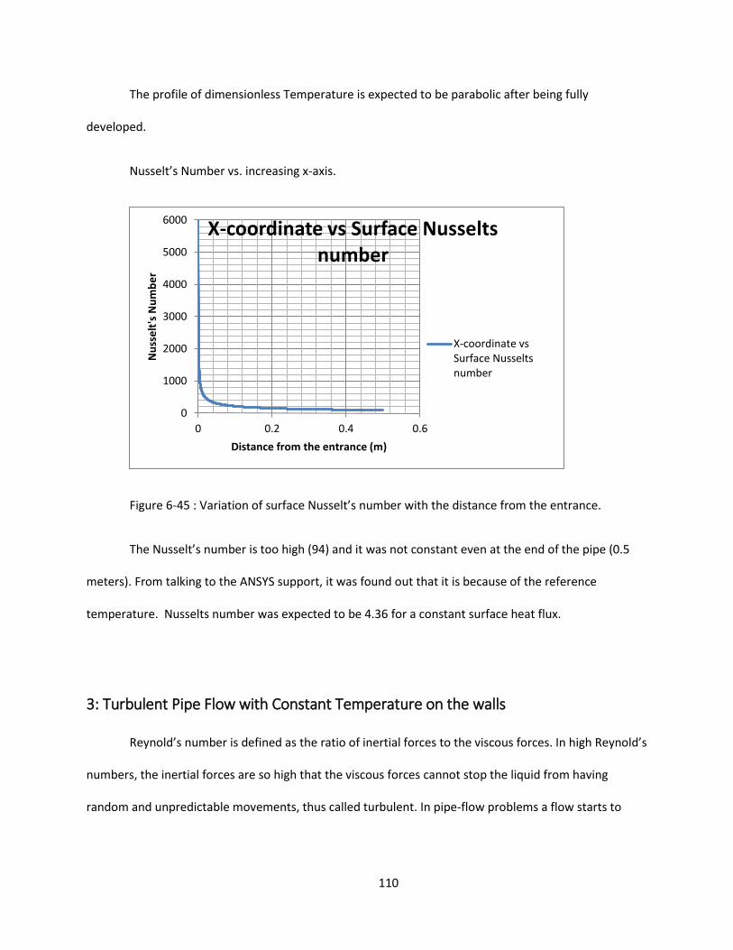
110

The profile of dimensionless Temperature is expected to be parabolic after being fully

developed.

Nusselt’s Number vs. increasing x-axis.

Figure 6-45 : Variation of surface Nusselt’s number with the distance from the entrance.

The Nusselt’s number is too high (94) and it was not constant even at the end of the pipe (0.5

meters). From talking to the ANSYS support, it was found out that it is because of the reference

temperature. Nusselts number was expected to be 4.36 for a constant surface heat flux.

3: Turbulent Pipe Flow with Constant Temperature on the walls

Reynold’s number is defined as the ratio of inertial forces to the viscous forces. In high Reynold’s

numbers, the inertial forces are so high that the viscous forces cannot stop the liquid from having

random and unpredictable movements, thus called turbulent. In pipe-flow problems a flow starts to

0

1000

2000

3000

4000

5000

6000

0 0.2 0.4 0.6

Nu

sse

lt's

Nu

mb

er

Distance from the entrance (m)

X-coordinate vs Surface Nusselts number

X-coordinate vs Surface Nusselts number

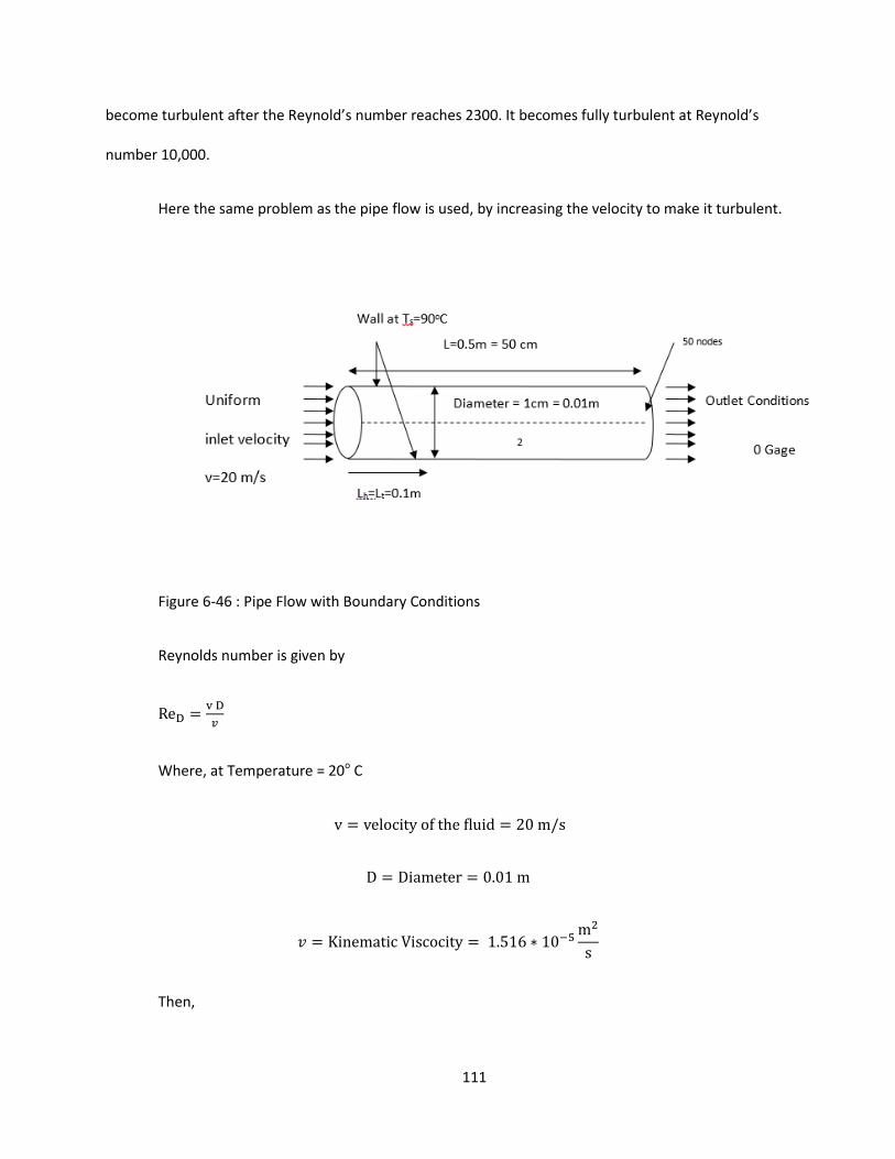
111

become turbulent after the Reynold’s number reaches 2300. It becomes fully turbulent at Reynold’s

number 10,000.

Here the same problem as the pipe flow is used, by increasing the velocity to make it turbulent.

Figure 6-46 : Pipe Flow with Boundary Conditions

Reynolds number is given by

Where, at Temperature = 20o C

Then,

112

So the Flow is Turbulent.

For Turbulent Flow, Both Hydrodynamic and thermal entry length is given by Lt=Lh=10D=0.1m.

A fluent model was ran to look at the entry length and study how the velocity profile changes.

Theory of fully developed turbulent velocity profile:

A fully developed turbulent flow in a pipe can be broken into three different sub-layers

(Munson):

Viscous sub layer is very close to the pipe wall and has a very dominant viscous shear stress. The

second layer is overlap region, and the third region is the outer region. In the outer region, turbulent

stress is dominant, while the overlap region is the region where the stress transforms from viscous to

turbulent. In the analysis of the turbulent flow, viscosity is very important in the viscous sub layer while

density of the flow is important in the outer layer.

The velocity profile is different in the viscous sub layer and the outer region. In viscous sublayer,

the velocity profile can be written in dimensionless form as

Where, y=R-r is the distance from the wall, ū is the time-averaged x-component of velocity and

u* = (Ƭw/ρ)1/2 is the friction velocity. Equation (5-20) is commonly known as the law of the wall.

In the Overlap region, the velocity is given by the relation

113

Similarly, the velocity in the outer region is given by the following expression:

Another common way to define the velocity profile in a turbulent flow is

N=7 is a commonly accepted value to define the velocity profile for turbulent flows. It needs to

be clear that the equation 5-23 does not precisely tell us velocity near the walls and at the center line,

however the approximate values are accepted.

The figure below clearly shows the difference between the laminar and turbulent flow in a pipe.

The velocity profile of the turbulent flow is much blunt towards the center.

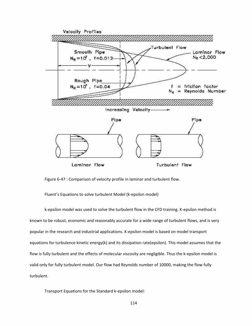
114

Figure 6-47 : Comparison of velocity profile in laminar and turbulent flow.

Fluent’s Equations to solve turbulent Model (k-epsilon model)

k-epsilon model was used to solve the turbulent flow in the CFD training. K-epsilon method is

known to be robust, economic and reasonably accurate for a wide range of turbulent flows, and is very

popular in the research and industrial applications. K-epsilon model is based on model transport

equations for turbulence kinetic energy(k) and its dissipation rate(epsilon). This model assumes that the

flow is fully turbulent and the effects of molecular viscosity are negligible. Thus the k-epsilon model is

valid only for fully turbulent model. Our flow had Reynolds number of 10000, making the flow fully

turbulent.

Transport Equations for the Standard k-epsilon model:

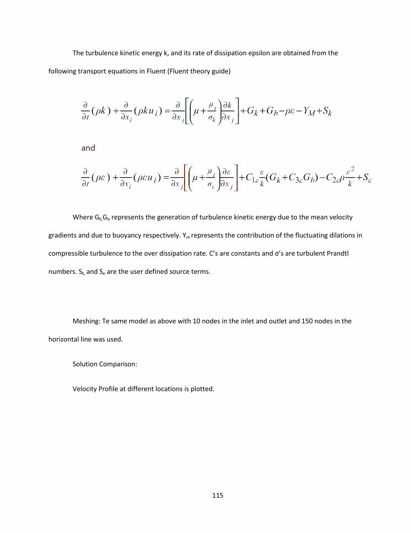
115

The turbulence kinetic energy k, and its rate of dissipation epsilon are obtained from the

following transport equations in Fluent (Fluent theory guide)

Where Gk,Gb represents the generation of turbulence kinetic energy due to the mean velocity

gradients and due to buoyancy respectively. Ym represents the contribution of the fluctuating dilations in

compressible turbulence to the over dissipation rate. C’s are constants and σ’s are turbulent Prandtl

numbers. Sk, and Se are the user defined source terms.

Meshing: Te same model as above with 10 nodes in the inlet and outlet and 150 nodes in the

horizontal line was used.

Solution Comparison:

Velocity Profile at different locations is plotted.

116

Figure 6-48 : Velocity Profiles of a turbulent Flow

The velocity profiles at different locations look about expected. The profiles of turbulent flow

are known to have nearly a straight line at the core region, and have significant velocity gradient in the

viscous sub layer.

Skin Friction Coefficient:

Figure 6-49: variation of Skin Friction Coefficient in turbulent flow

117

The curve for skin friction coefficient doesn’t look very convincing, as it doesn’t remain constant

after the hydrodynamic boundary layers meet. This is mainly because the mesh is not dense enough to

properly capture the skin friction near the wall. A denser mesh, or proper wall function should be used

closer to the wall in the future.

118