INVESTIGATION OF HEAT TRANSFER AND MASS

TRANSFER PARAMETERS IN A CONVECTION OVEN

FOR MODEL FOODS Submitted by

Chandana Mysore Somashekar

(ch7445my-s@student.lu.se)

Department of Food Technology, Engineering and Nutrition

Faculty of Engineering, LTH

Lund University

Supervisor: Andreas Håkansson

Examiner: Marilyn Rayner

August 2020

LUND-SWEDEN

Abstract

Forced air convection systems are the most preferred design of choice in many of the

industrial-scale convection ovens. In this study, experimental investigation on convective heat

transfer and mass transfer within a forced air convection oven was performed at different

oven temperatures (100℃, 110℃ and 120℃) and at flow velocity (2m/s, 3m/s and 4m/s)

using potato slices (10*10*60mm) as model food. The Yıldız et al., 2007 approach with slight

modification was applied to estimate the effective convective heat transfer and mass transfer

coefficient during convection frying. In addition to the experimental approach, the empirical

correlation method was also used to calculate the convective heat transfer and mass transfer

coefficient and compared with the coefficient values obtained from the experimental

method. The effective heat transfer and mass transfer coefficient obtained from the Yıldız et

al., 2007 method was found to be almost constant with increasing oven temperature.

However, with increasing flow velocity the effective heat transfer coefficient increased but

the influence of flow velocity on effective mass transfer coefficient was not significant. The

comparison of the coefficient values obtained from the experimental method and the

empirical correlations showed that the experimental method yields quite low values than the

empirical method.

Acknowledgements

It gives me immense pleasure to present this section as a tribute to all the people who

encouraged and supported me during this degree project.

This study was carried out as a degree project in food engineering at the Department of Food

Technology, Engineering and Nutrition under the supervision of Associate Professor Andreas

Håkansson. The examiner of the project is Professor Marilyn Rayner, Department of Food

Technology, Engineering and Nutrition.

Firstly, I would like to express my sincere gratitude to my supervisor Prof. Andreas Håkansson

for giving me the opportunity to carry out this project and guiding me by providing his

valuable suggestions and feedback throughout the project. Secondly, I would like to thank

Grant Thamkaew Doctoral student at Department of Food Technology, Engineering and

Nutrition for providing instructions required to operate the convection oven and cooperating

during the entire project.

Finally, I thank Almighty for being able to give my best and my special thanks go to my parents

and friends for their constant moral support and encouragement which helped me to

successfully completion this project.

Index

1. Introduction ........................................................................................................................... 1

1.2 Background ...................................................................................................................... 1

1.3 Objectives ........................................................................................................................ 1

2. Theory .................................................................................................................................... 2

2.1 Heat transfer .................................................................................................................... 2

2.2 Mass transfer ................................................................................................................... 3

2.3 Simultaneous heat and mass transfer ............................................................................ 3

2.4 Methods to determine the convective heat transfer and mass transfer parameters .. 4

2.4.1 Yıldız et al. (2007) method for determination of heat transfer coefficient ............ 4

2.4.2 Yıldız et al. (2007) method for determination of mass transfer coefficient ........... 5

2.4.3 Determination of heat transfer coefficient using dimensionless correlations ...... 6

2.4.4 Analogy between heat and mass transfer - Chilton and Colburn analogy ............. 9

2.4.5 Determination of mass transfer coefficient using dimensionless correlations ..... 9

3. Materials and Methods ....................................................................................................... 11

3.1 Apparatus ....................................................................................................................... 11

3.2 Sample preparation ....................................................................................................... 11

3.3 Experimental setup........................................................................................................ 11

3.4 Experimental procedure ................................................................................................ 13

4.1 Primary results of mass loss and centre temperature increase .................................. 14

4.2 Determination of effective heat transfer coefficient using Yıldız method ................. 19

4.3 Determination of effective mass transfer coefficient using Yıldız method ................ 21

4.4 Comparison of the experimentally determined h and Km values with the empirically

predicted values using correlations .................................................................................... 23

4.4.1 Heat transfer coefficient ......................................................................................... 23

4.4.2 Mass transfer coefficient ........................................................................................ 23

6. Conclusion ........................................................................................................................... 25

7. Future Research ................................................................................................................... 26

References ............................................................................................................................... 27

Appendices .............................................................................................................................. 28

Appendix A: Thermophysical properties of potato.(Yıldız et al. (2007) ............................ 28

Appendix B: Constants for the circular cylinder in cross flow.( Bergman and Lavine,

2018) .................................................................................................................................... 29

Appendix C: Determination of diffusivity coefficient for theoretical estimation of mass

transfer coefficient at different oven temperatures. (Brodkey and Hershey, 1988) ........ 30

Appendix D: Calculations of the heat transfer coefficient using empirical correlations .. 31

Appendix E: Calculations of the mass transfer coefficient using correlations analogous to

the heat transfer correlations ............................................................................................. 33

Appendix F: Additional pictures of experimental setup .................................................... 35

Nomenclature

A Surface area (m2) Bi Biot number

C(x,t) Moisture content at any point and any time (kg/kg solid)

C*∞ Moisture content in the air (kg/m3)

C*sur Moisture content at the surface (kg/m3)

C∞ Moisture content of the air in the oven (kg/kg solid)

Ci Initial uniform moisture content of the product (℃)

Cp Specific heat (J/kgK)

D Moisture diffusivity (m2/s)

dc Characteristic dimension

h Heat transfer coefficient (W/m2K) heff Effective heat transfer coefficient (W/m2K) k Thermal conductivity

km Mass transfer coefficient (m/s)

L Half thickness (m)

mB Mass flux (kg/s)

NNu Nusselt number NPr Prandtl number NRe Reynolds number NSc Schmidt number NSh Sherwood number Q Heat flux (W) St Stanton number t Time (s)

T(x,t) Temperature at any point and any time (℃)

T∞ Temperature of the air in the oven (℃)

Tair Temperature of the air (℃)

Tf Film temperature (℃)

Ti Initial uniform temperature of the product (℃)

Tsur Temperature at the product surface (℃)

u Velocity (m/s) V Volume (m3) x Location where temperature is measured in infinite slab (0 ≤ x ≤ L) y Location where temperature is measured in infinite slab (0 ≤ y ≤ L) α Thermal diffusivity (m2/s) ρ Density (kg/m3) 𝚫Hevp Enthalpy of vaporization (kJ/mol) ⅆ𝒎

ⅆ𝒕 Rate of mass reduction (kg/s)

µ Viscosity (Ns/m2) µb Viscosity of the fluid(air) (Ns/m2) µw Viscosity at the solid surface (Ns/m2)

1

1. Introduction

1.2 Background

A forced convection oven is popular cooking equipment used in the home and in the food

industries to produce baked products, meat, dried and fried products. There are various types

of forced convection ovens available in the market. In these ovens, food is heated by hot air

that is circulated around the product by a fan fit to the oven wall. Heat is transferred to the

product through radiation and convective heat transfer by the circulating air, at same time

water from the product surface is transferred to the air due to evaporation (Skjoldebrand,

1980). In many solid foods processes heat transfer is analogous to mass transfer and there is

a strong coupling between heat and moisture transfer. Such a process is called as a coupled

heat and mass transfer. This coupled heat and mass transfer play an important role in many

solid food processes like baking, drying, and frying (Feyissa, 2011).

During frying in a convection oven, the product is heated by air at high temperature to induce

changes in the product like water evaporation, crust formation, browning, protein

denaturation and inactivation of enzymes and various microorganisms. These changes are

desirable and renders the product with appealing colour, flavour, texture, and shelf life.

However, some undesirable transformation may also occur for example, the formation of

acrylamide, which is regarded as a potentially carcinogen. The acrylamide formation depends

upon temperature and heating time (Feyissa, 2011). Mass transfer in convection oven refers

to the loss of water content from solid food which has a major influence on the chemical and

physical properties that describes the desired food quality and safety (Thorvaldsson and

Skjöldebrand, 1996). Therefore, it is essential to have a thorough quantitative understanding

of mass transfer and heat transfer parameters during cooking food. Further, understanding

of process parameters helps to identify and apply optimal processing conditions to obtain

desired final product quality and has an important role in scale up at industry.

Several studies on heat and mass transfer coefficients and the effects of influencing factors

are present in the literature. (Skjoldebrand, 1980; Yıldız et al., 2007; Safari et al., 2018). These

studies have contributed a lot of useful information about heat and mass transfer using

different techniques. However, the study of heat transfer and mass transfer parameters in a

forced convection oven is limited.

1.3 Objectives

Investigation of effective heat transfer and mass transfer coefficient at different

temperatures and flow(air) velocity using the Yildiz et al. (2007) approach in a forced air

convection oven for cuboidal model foods.

Discuss and conclude on how the effective heat transfer and mass transfer coefficients

vary with increasing oven temperature and flow(air) velocity.

2

Compare the experimentally obtained coefficient values (using method described in Yıldız

et al., 2007) with the values from the empirical correlations and discuss the variations.

2. Theory

2.1 Heat transfer

Heat transfer is the movement of energy from one point to another by the virtue of difference

in temperature. This temperature difference is the driving force which establishes the rate of

heat transfer (Toledo, 2007). Heat transfer is of two types, external heat transfer and internal

heat transfer. The former takes place between the heating medium and the solid food and

the latter takes place within the solid food itself. A solid food and a heating medium

exchanges heat at their boundaries by the mechanism of conduction, convection, or radiation

(Feyissa, 2011). When the heat is transferred by the molecule that move from one point to

another and exchanges energy with another molecule in other location, the process is called

convection heat transfer (Toledo, 2007). There are two types of convective heat transfer

depending on the flow characteristics of the heating medium: forced convection and free

convection. In forced convection, the flow is artificially induced by blowing air or pumping

liquid on the heating or cooling surface. In contrast, free convection occurs due to density and

viscosity changes associated with the temperature difference in the fluid (Heldman and Lund,

2007). Convective heat transfer is a major mode of heat transfer between the surface of a

solid food and the surrounding heating medium, used in many processes like baking, roasting

and frying in a convection oven (Heldman and Lund, 2007; Feyissa, 2011). In domestic

convection ovens, radiation mode of heat transfer is considered to have major contribution.

In case of convection heat transfer, the rate of heat transfer is proportional to the surface

area in contact with the heating medium and the temperature difference and is expressed as,

Q = h*A*(Tair-Tsur) Eq. (1)

where ‘h’ is the heat transfer coefficient(W·m−2·K−1), ‘A’ is the area of the heating medium –

solid interface where heat is being transferred (m2), Tair is the temperature of the air in the

oven (K), Tsuris the surface temperature of the solid food (K). Convective heat transfer during

forced air convection is represented as heat transfer through a thin film of air that possess a

temperature gradient, at the air-solid surface interface. The thin air film is a boundary layer

that resists the heat flow between the air stream and the solid food. The reduction in the

thickness of the boundary layer will promote the heat transfer to the solid food. The heat

transfer coefficient depends on the thermophysical properties of the fluid, the velocity of the

fluid flow, geometry of the solid undergoing heating or cooling and the roughness of the

surface in contact with the fluid flow. The convective heat transfer coefficient, h, has been

measured experimentally by several researchers using different methods for a variety of

operating conditions. Empirical correlations have been developed to estimate the convective

heat transfer coefficient for different operating conditions (Singh and Heldman, 2014).

3

2.2 Mass transfer

Mass transfer in food systems is referred as, the migration of a constituent of a fluid or a

component of a mixture. The migration occurs because of changes in the physical equilibrium

of the system caused by the concentration differences. It can occur within one phase or may

involve transfer from one phase to another. Mass transfer involves both diffusion at a

molecular level and bulk transport of mass due to convection flow (Singh and Heldman, 2014).

Diffusion is the process by which matter is transported from one part of the system to another

due to random molecular motion (Toledo, 2007). The diffusion process is described

mathematically using Fick’s law of diffusion, which states that the mass flux per unit area of

a component is proportional to its concentration gradient. Convection enhances the transport

of components due to concentration gradient as a result, the mass flux of the component will

be higher than would occur by molecular diffusion (Singh and Heldman, 2014). During forced

convection, air flows over a wet surface and water is transferred from the surface to the air

which is analogous to convection heat transfer. Therefore, the driving force for mass transfer

is a concentration difference, and the proportionality constant between the mass flux and the

driving force is the mass transfer coefficient. �̇�𝐵

𝐴= 𝑘𝑚 (C*sur – C*∞) Eq. (2)

‘km’ is convective mass transfer coefficient defined as, the rate of mass transfer per unit area

per unit concentration difference. ‘mB’ is the mass flux (kg/s), ‘C*’ is moisture content in (kg

water/m3), ‘A’ is area of the surface through which water is transferred to air (m2). The

determination of mass transfer coefficient is analogous to that of heat transfer coefficient,

involving the dimensionless analysis. (Singh and Heldman, 2014).

2.3 Simultaneous heat and mass transfer

Convection cooking involves the simultaneous heat and mass transfer. Heat is transferred

mainly by convection from air to the product surface, and by conduction from the surface

toward the product centre. Meanwhile, moisture diffuses outward toward the product

surface, and is vaporized. At the product surface, simultaneous heat and mass transfer is

controlled by convective processes(Singh and Heldman, 2014). Heat transferred from the air

to the product surface results in evaporation of water from the surface. This evaporation

process requires heat energy, which is taken away by the molecules when they convert from

liquid phase to the gas phase and escape from the surface. Since the molecules take away

heat while leaving the surface, this has a cooling effect on the surface which is referred to as

evaporation cooling effect. This phenomenon is mainly because of coupling between heat

transfer (air to product) and mass transfer(product to air) (Toledo, 2007). There is also a

coupling in the other direction since the heat transfer influences the fluid (air) temperature

which influences the thermophysical properties of the fluid(air). This type of coupling effect

is mostly observed in food processes involving air flow. For example, freezing, thawing,

dehydrating, and cooking of food products (Kondjoyan & Daudin, 1997). These coupling

4

effects introduce the concept of effective heat transfer coefficient. Effective heat transfer

coefficient is a combination of convective heat transfer coefficient and evaporative cooling.

While determining effective heat transfer coefficient, heat exchanged by radiation or by

phase change when it occurs(evaporation cooling effect) is considered in addition to the heat

exchanged by convection (Kondjoyan & Daudin, 1997). The effective heat transfer coefficient

provides the heat interaction between the product and the heat transfer fluid during heat or

cooling processes (Chen et al., 1999). It can be represented as,

heff ∗ A ∗ (Tair -Tsur) = h * A * (Tair -Tsur) + ΔHvap* ⅆ𝑚

ⅆ𝑡+ 𝑟𝑎𝑑𝑖𝑎𝑡𝑖𝑜𝑛 Eq.(3)

2.4 Methods to determine the convective heat transfer and mass transfer parameters

Over the year’s researchers have used different methods to determine the heat transfer and

mass transfer parameters in a various operating condition. There is no standard method for

measuring heat and mass transfer coefficients during forced convection cooking (J.K. Carson

et al., 2006; Sablani, 2009). In this study, we have used the technique discussed in Yıldız et al.

(2007) for immersion frying to calculate the heat and mass transfer coefficients during forced

convection cooking. In Yıldız et al. (2007) method the experimental data were used to

determine the heat and mass transfer parameters during frying from the dimensionless

temperature and concentration ratio plots, respectively. Another approach used in this study

is, calculating heat transfer and mass transfer coefficient using empirical equations or

correlations. This approach is applicable when appropriate correlations suitable for the type

of process and food of interest are available.

2.4.1 Yıldız et al. (2007) method for determination of heat transfer coefficient

In this method, the temperature in the centre of the sample is measured as a function of time

and used together with an analytical solution to back-calculate the rate of external heat

transfer. Eq. (4) is the partial differential equation for heat conduction.

𝜕2𝑇

𝜕𝑥2=

1

𝛼

𝜕𝑇

𝜕𝑡 , 0 ≤ 𝑥 ≤ 𝐿 for t > 0 Eq. (4)

Eq. (4) is solved by applying boundary conditions given in Eq. (5)

Eq. (5)

𝜕𝑇

𝜕𝑥|

𝑥=0= 0 −𝑘

𝜕𝑇

𝜕𝑥|

𝑥=𝐿= ℎ(𝑇|𝑥=𝐿 − 𝑇∞) 𝑇|𝑡=0 = 𝑇𝑖

Eq. (6) is the analytical solution of Eq. (4).

(𝑇(𝑥,𝑡)−𝑇∞

𝑇𝑖−𝑇∞) = ∑

2 𝑠𝑖𝑛 𝜇𝑛

𝜇𝑛+𝑠𝑖𝑛 𝜇𝑛 𝑐𝑜𝑠 𝜇𝑛

∞

𝑛=1⋅ cos (𝜇𝑛

𝑥

𝐿) exp (−𝜇𝑛

2 𝛼𝑡

𝐿2) Eq. (6)

𝐵𝑖 = 𝜇𝑛 tan 𝜇𝑛 Eq. (6b)

5

Eq. (6) gives temperature as a function of time at any point in an infinite slab.

After a certain interval of processing time where the Fourier number (αt/L2) is greater than

0.1, Eq. (6) converges to the first term in the series. The first term solution for a cuboidal

shaped solid is obtained by the product of the first term solutions of three infinite slabs of the

same thickness. Eq. (7) represents the solution for a cuboidal shaped food.

(𝑇(𝑥,𝑡)−𝑇∞

𝑇𝑖−𝑇∞) ⋅ (

𝑇(𝑦,𝑡)−𝑇∞

𝑇𝑖−𝑇∞) = A exp (−2𝜇1

2 𝛼𝑡

𝐿2) Eq. (7)

Where A = (2 𝑠𝑖𝑛 𝜇1

𝜇1+𝑠𝑖𝑛 𝜇1 𝑐𝑜𝑠 𝜇1)

2

⋅ cos (𝜇1𝑥

𝐿) ⋅ cos (𝜇1

𝑦

𝐿)

Taking natural logarithm on both sides of Eq. (7) gives Eq. (8)

𝑙𝑛 (𝑇(𝑥,𝑦,𝑡)−𝑇∞

𝑇𝑖−𝑇∞) = ln A - 2𝜇1

2 𝛼𝑡

𝐿2 Eq. (8)

The slope of linear section of 𝑙𝑛 (𝑇(𝑥,𝑦,𝑡)−𝑇∞

𝑇𝑖−𝑇∞) versus time is used in solving Eq. (8) for µ1 value.

The thermal diffusivity α is calculated from the thermophysical properties of food

sample(potato) presented in table 1.1 in Appendix A. Further the heat transfer coefficient, h,

and heat transfer Biot number (Bih) are determined by using Eq. (9) and Eq. (10) where k is

the thermal conductivity of potato in (W/mK).

𝐵𝑖ℎ = 𝜇1 tan 𝜇1 Eq. (9)

𝐵𝑖ℎ = ℎ𝐿

𝑘 Eq. (10)

2.4.2 Yıldız et al. (2007) method for determination of mass transfer coefficient

The mass transfer coefficient is determined from the dimensionless concentration versus time plots. This approach relies on measuring moisture content of the sample over time and solving differential equation (Eq. (11)) using boundary conditions in Eq. (12)

𝜕2𝐶

𝜕𝑥2 =1

𝐷

𝜕𝐶

𝜕𝑡 , 0 ≤ 𝑥 ≤ 𝐿 for t > 0 Eq. (11)

𝜕𝐶

𝜕𝑥|

𝑥=0= 0 −𝐷

𝜕𝐶

𝜕𝑥|

𝑥=𝐿= 𝑘𝐶(𝐶|𝑥=𝐿 − 𝐶∞) 𝐶|𝑡=0 = 𝐶𝑖 Eq. (12)

Eq. (13) is the solution of differential equation(Eq. (11)) that gives concentration as a function of time and location for an infinite plate.

(𝐶(𝑥,𝑡)−𝐶∞

𝐶𝑖−𝐶∞) =

2 sin2 𝜇1

𝜇1[𝑢1+sin 𝜇1∗ cos 𝜇1] ⋅ cos (𝜇𝑛

𝑥

𝐿) exp (−𝜇𝑛

2 𝐷𝑡

𝐿2) Eq. (13)

For a long processing time, Fo = αt/L2 is greater than 0.1 and the first term of the differential

equation solution(Eq. (13)) is enough to give accurate results. Note that the time interval for

6

which the value of Fourier number(αt/L2 ) is greater than 0.1 is different for mass and heat

transfer.

By integrating Eq.(13) throughout the whole volume (1

𝑉∫ 𝐶(𝑥, 𝑡) 𝑑𝑉

𝑉

0) , the equation for

average moisture concentration in a cuboid shaped solid(Eq. (14)) was obtained.

(𝐶̅(𝑡) − 𝐶∞

𝐶𝑖 − 𝐶∞̅̅ ̅̅ ̅̅ ̅̅ ̅̅ ) =

2 sin2 𝜇1

𝜇1[𝑢1+sin 𝜇1∗ cos 𝜇1]exp (−𝜇1

2 𝐷𝑡

𝐿2) Eq. (14)

𝐶̅(𝑡) is the average moisture content at time t in (kg/kg solids)

Taking the natural logarithm on both the sides of Eq. (14) gives the following equation:

𝑙𝑛 (𝐶̅(𝑡) − 𝐶∞

𝐶𝑖 − 𝐶∞̅̅ ̅̅ ̅̅ ̅̅ ̅̅ ) = 2 𝑙𝑛 𝐸 − 2𝜇1

2 𝐷𝑡

𝐿2 Eq. (15)

Where, E = 2 sin2 𝜇1

𝜇1[𝑢1+sin 𝜇1∗ cos 𝜇1]

According to Yıldız et al. (2007) method, a plot of 𝑙𝑛 (𝐶̅(𝑡) − 𝐶∞

𝐶𝑖 − 𝐶∞̅̅ ̅̅ ̅̅ ̅̅ ̅̅

) against time is used to

determine the moisture diffusivity, D (m2/s) and µ1 from the slope and the intercept of the

plotted curve, respectively . However, preliminary investigations showed that the method

was extremely sensitive to small deviations in the measured data. Hence, in this study a bit

modified method similar to the one in Yıldız et al. (2007) for heat transfer is used. By applying

similar approach as in heat transfer, a plot of 𝑙𝑛 (𝐶̅(𝑡) − 𝐶∞

𝐶𝑖 − 𝐶∞̅̅ ̅̅ ̅̅ ̅̅ ̅̅

) against time is used to determine

µ1 value, from the slope of the plotted curve. The moisture diffusivity, D (m2/s) is assumed to

be constant and the value is obtained from Yıldız et al. (2007) . After determining µ1, the mass

transfer Biot number (Bim) and mass transfer coefficient (km) were obtained from Eq. (16).

𝐵𝑖𝑚 = 𝜇1 𝑡𝑎𝑛 𝜇1 =𝑘𝑚𝐿

𝐷 Eq. (16)

2.4.3 Determination of heat transfer coefficient using dimensionless correlations

Convective heat transfer coefficient, ‘h’, can be estimated from dimensionless correlations

based on the velocity and thermophysical properties of the air and the geometrical shape and

temperature of the food. The general correlation between the dimension less numbers for

forced convection is,

NNu = f(NRe, NPr) Eq. (17)

Where, NNu is Nusselt number ,NPr is the Prandtl number and NRe is Reynold number.

The Nusselt number,

NNu = ℎ ⅆ𝑐

𝑘 Eq. (18)

7

Where h is convective heat-transfer coefficient(W/[m2K]), dc is the characteristic dimension

(m), k is thermal conductivity of fluid (W/[mK]) is defined as the ratio of the characteristic

dimension of a system and the thickness of the boundary layer of fluid that would transmit

heat by conduction at the same rate as that calculated using the heat transfer coefficient. The

Reynolds number,

NRe = 𝜌𝑢 ⅆ𝑐

𝜇 Eq. (19)

where ρ is density of fluid (kg/m3), u is velocity of fluid (m/s), μ is viscosity (Pa s) is described

as the ratio of inertial forces to the frictional forces. Prandtl number is the ratio of rate of

momentum exchange between molecules and the rate of energy exchange between

molecules that lead to the transfer of heat,

NPr = 𝜇 𝐶𝑝

𝑘 Eq. (20)

Where Cp is specific heat (J/ [kg K]) and k is thermal conductivity of fluid (W/[mK]).

With a basic understanding of these three dimensionless numbers, correlations for

determining ‘h’, convective heat-transfer coefficient(W/[m2K]) during various operating

conditions are obtained. Different correlations are obtained, depending on whether the flow

is laminar or turbulent. Some of the correlations that are relevant to the operating conditions

of this study are, flow over cylinder of noncircular cross section, flow around a cylinder and

flow around a sphere. (Singh and Heldman, 2014; Toledo, 2007; Bergman and Lavine, 2018)

Eq.(21) is the Nusselt correlation for predicting heat transfer coefficient value for flow over

cylinders of noncircular cross section with characteristic length dc (m) (‘dc’ is half thickness for

cuboid geometry) and all thermophysical properties of fluid(air) evaluated at film

temperature, Tf =[ (Ts+Tair)/2]. Figure 1 is a schematic illustration of the fluid flow around a

cylinder of noncircular cross section(cuboid) giving rise to the external convective heat

transfer described by Eq. (21). The constant values are taken from table 1.2 appendix A

(Bergman and Lavine, 2018).

NNu = C(NRe)m(NPr)1/3 Eq. (21)

8

Figure 1. Illustration of flow over cylinders of noncircular cross section

The Nusselt correlation for determining the convective heat transfer coefficient for flow

around a sphere, when the single sphere is heated or cooled is,

NNu = 2 + 0.6(NRe)0.5(NPr)0.33 Eq. (22)

for 1 < NRe < 70000 and 0.6 < NPr < 400

where the characteristic dimension, dc, is the outside diameter of the sphere. The fluid

properties are evaluated at the film temperature Tf (Singh and Heldman, 2014). Figure 2

shows an illustration of the fluid flow around spherical and cylindrical object which results in

the external convective heat transfer described by Eq. (22) and Eq. (23) respectively.

Figure 2.Illustration of flow around sphere and cylinder

Eq. (23) is the Nusselt number correlation for flow around a cylinder.

NNu = (0.4NRe1/2 + 0.06NRe

2/3 )(NPr)0.4(𝜇𝑏

𝜇𝑤)

1/4

Eq. (23)

In the range 1.0 < Re <1.0*105, 0.67 < Pr < 300 and 0.25 < 𝜇𝑏

𝜇𝑤 < 5.2

All fluid properties are evaluated at the film temperature Tf ,except 𝜇𝑤 , which is evaluated at

wall temperature and the characteristic dimension, dc, is the outer diameter of the

cylinder.(Bird, 2002)

9

In this study Eq. (21), Eq. (22) and Eq. (23) are used to determine to heat transfer coefficient,

h, during forced convection cooking of a cuboidal shaped potato slices and the value obtained

are compared to with the experimentally determined results.

2.4.4 Analogy between heat and mass transfer - Chilton and Colburn analogy

The Chilton-Colburn analogy states that there is a relationship between the rate of convective

heat and mass transfer, provided a number of assumptions are met (e.g., that all physical

properties of the food and the air remains constant with respect to time).

St ⋅ Pr2/3 = Stm ⋅ Sc2/3 Eq. (24)

where St and Stm are the heat transfer Stanton number and mass transfer Stanton number,

respectively.

St = Nu

Re⋅Pr Eq. (25)

Stm = Sh

Re⋅Sc Eq. (26)

By substituting the equations 25 & 26 in Eq. (24)

Nu

Re⋅Pr . Pr2/3 =

Sh

Re⋅Sc . Sc2/3 Eq. (27)

Nu ⋅ Pr-1/3 = Sh ⋅ Sc-1/3 Eq. (28)

Sh = Nu ⋅ Pr-1/3⋅ Sc1/3 Eq. (29)

By substituting the Nusselt number from the heat transfer correlation in Eq. (29) we get the

Sherwood number. The mass transfer coefficient is calculated from the Sherwood number.

2.4.5 Determination of mass transfer coefficient using dimensionless correlations

Convective mass transfer coefficient ‘km’ is determined using dimensionless correlations,

analogous to the correlations used in convective heat transfer coefficient estimation. some

of the important dimensionless numbers involved in determination of mass transfer

coefficient are, Sherwood number (NSh), Schmidt number (NSc) and Reynold number (NRe).

The functional relationship that correlate these dimensional numbers for forced convection

is,

NSh = f(NRe, NSc) Eq. (30)

NSh = 𝑘𝑚⋅ ⅆ𝐶

𝐷𝐴𝐵 Eq. (31)

10

km is the mass transfer coefficient (m/s), dc is the characteristic dimension (m), DAB is

diffusivity for component A in fluid B.

NRe = 𝜌⋅𝑢⋅ⅆ𝑐

𝜇 Eq. (32)

ρ is density of fluid (kg/m3), u is velocity of fluid (m/s), μ is viscosity (Pa s).

NSc = 𝜇

𝜌𝐷𝐴𝐵 Eq. (33)

As the heat transfer is analogous to mass transfer, the Chilton-Colburn analogy described in section 2.4.4 is used to obtain the mass transfer coefficient value from the heat transfer correlations. By Applying the Chilton and Colburn analogy, Eq. (34) gives the convective mass transfer

coefficient, (km) for flow over cylinders of noncircular cross section

NSh = C(NRe)m⋅ NSc1/3 Eq. (34)

All fluid properties are evaluated at the film temperature Tf and dc for a cuboid shaped solid

is half the thickness. The values of C and m, are obtained from table 1.1 appendix A.

The dimensionless correlation for estimating the mass transfer coefficient in case of flow over

spherical objects is,

NSh = 2 + 0.6(NRe)0.5⋅ NSc1/3 Eq. (35)

where the characteristic dimension, dc, is the outer diameter of the sphere. The fluid

properties are evaluated at the film temperature Tf.

The dimensionless correlation for estimating the mass transfer coefficient for flow around a

cylinder is given by Eq. (36),

NSh = (0.4NRe1/2+ 0.06NRe

2/3 )(NPr)0.4(𝜇𝑏

𝜇𝑤)

1/4

⋅ NPr-1/3 ⋅ NSc

1/3 Eq. (36)

The characteristic dimension, dc, is the outer diameter of the cylinder and the fluid properties

are evaluated at the film temperature Tf ,except 𝜇𝑤, which is evaluated at wall temperature.

11

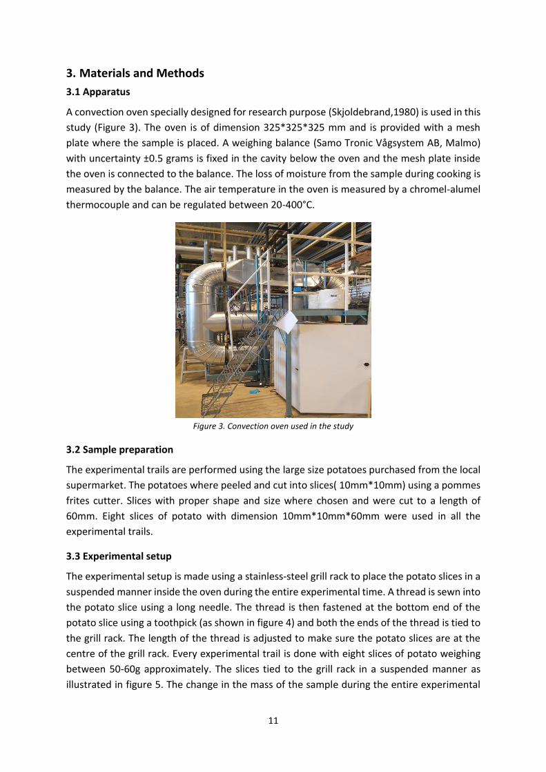
3. Materials and Methods 3.1 Apparatus

A convection oven specially designed for research purpose (Skjoldebrand,1980) is used in this

study (Figure 3). The oven is of dimension 325*325*325 mm and is provided with a mesh

plate where the sample is placed. A weighing balance (Samo Tronic Vågsystem AB, Malmo)

with uncertainty ±0.5 grams is fixed in the cavity below the oven and the mesh plate inside

the oven is connected to the balance. The loss of moisture from the sample during cooking is

measured by the balance. The air temperature in the oven is measured by a chromel-alumel

thermocouple and can be regulated between 20-400°C.

Figure 3. Convection oven used in the study

3.2 Sample preparation

The experimental trails are performed using the large size potatoes purchased from the local

supermarket. The potatoes where peeled and cut into slices( 10mm*10mm) using a pommes

frites cutter. Slices with proper shape and size where chosen and were cut to a length of

60mm. Eight slices of potato with dimension 10mm*10mm*60mm were used in all the

experimental trails.

3.3 Experimental setup

The experimental setup is made using a stainless-steel grill rack to place the potato slices in a

suspended manner inside the oven during the entire experimental time. A thread is sewn into

the potato slice using a long needle. The thread is then fastened at the bottom end of the

potato slice using a toothpick (as shown in figure 4) and both the ends of the thread is tied to

the grill rack. The length of the thread is adjusted to make sure the potato slices are at the

centre of the grill rack. Every experimental trail is done with eight slices of potato weighing

between 50-60g approximately. The slices tied to the grill rack in a suspended manner as

illustrated in figure 5. The change in the mass of the sample during the entire experimental

12

time is recorded by connecting the digital balance to the computer, logging one value per

second.

In the experiments involving recording of temperature change in the sample, type-k

thermocouples were used. The thermocouple is sewn into two potato slices out of eight using

a long needle and sewing thread, making sure that the thermocouple is at the centre of the

potato slice. The thread is then fastened using a toothpick and tied to the grill rack. The

pictures of the experimental setup with the thermocouple inserted inside the potato slices

can be found in appendix F. The centre temperature of the sample during the experiment was

recorded by connecting the thermocouple data logger (Pico technology, Eaton Socon, UK) to

a computer with the logging software, logging one value per second.

Figure 4.slices of potato with a thread sewn into each piece and fastened at the bottom using a toothpick.

Figure 5. The pieces of potato tied at the centre of the stainless-steel grill rack with the help of the thread that is sewn into each piece.

13

3.4 Experimental procedure

The weight of empty stainless-steel grill rack is recorded and then weighted again along with

the potato slices just before placing it inside the oven. The initial mass of the sample is

calculated by subtracting the mass of the empty grill rack from the mass of grill rack with the

sample. The oven temperature and air velocity were set and allowed to stabilize for 45min

before placing the sample in the oven. Once the sample was place inside the oven the

temperature logging and mass logging were started. The schematic representation of the

experimental setup is shown in figure6. The runtime for each trial was set to 7200s so that

adequate amount of data is recorded. The experimental raw data is retrieved, and

calculations are done following the method in section 2.4.1 and section 2.4.2 to estimate the

heat transfer coefficient and mass transfer coefficient values using Microsoft Excel.

Figure 6. Schematic representation of the experimental setup

The experiments are performed with minimum 3 replicates for each set of condition as

represented in table 1. The experimental data of both heat and mass transfer can be recorded

simultaneously.

Table 1. Experimental trails performed

Convection cooking with operating conditions (temperature and air velocity)

Replicates

100℃, 3m/s 4

110℃, 3m/s 4

120℃, 3m/s 3

2m/s, 110℃ 4

3m/s, 110℃ 3

4m/s, 110℃ 3

14

4. Results and Discussion

4.1 Primary results of mass loss and centre temperature increase

The experimental data for the product centre temperature and mass change was recorded

simultaneously throughout the run time. Figure 7 is an example of experimental results

showing the centre temperature and mass change profile for an oven temperature set 120℃

and air velocity 3m/s.

Figure 7. change in the centre temperature and mass of the sample versus time during

forced convection cooking at 120℃ and 3 m/s air velocity.

We can observe in figure 7 the temperature is increasing and the mass is decreasing with

time, the increasing temperature profile is because of heat transfer from the air to the sample

and the decreasing mass profile is due to the mass transfer from the sample to the air. Note

that the temperature increases up to the boiling point of water (100℃) where it then remains

almost constant for an extended period(similar to constant-rate period in drying kinetics).

This is expected due to the evaporation cooling effect. After some time, the temperature

again rises as most of the water is evaporated and the energy is utilized to heat the sample

(falling-rate drying period). The mass curve of the sample decreases continuously until certain

time (t = 5500 s, approximately from the plot) and then flatten. At this point, there is very

negligible or no mass transfer to the air.

It can be interpreted from the plot that, the flattening of the mass curve after a long

processing time (t>5500 s, approximately from the plot) is because of very less or no moisture

content present in the sample. At this point most of the water from the sample would have

been evaporated(falling-rate drying period) and the sample is almost dry.

0

20

40

60

80

100

120

140

265

270

275

280

285

290

295

300

305

310

315

320

0 2000 4000 6000 8000

Tem

per

atu

re [

℃]

Mas

s [k

g]

Time[s]weight [kg] Temperature

15

Figure 8 represents the plot of centre temperature of food sample versus time recorded

during experimental run for three different oven temperatures.

Figure 8. Temperature profile of the sample at three different oven temperature

As we can see from the figure 8, the temperature of the sample increases faster when the

oven temperature is higher. The higher the set temperature of the oven the greater is the

temperature gradient which is driving force for heat transfer. Meaning that heat transfer is

more at higher temperatures. From the plot it is evident that the time required for the centre

temperature of the sample to reach boiling point of water is less when the oven temperature

is set to 120℃ than the time required when the oven temperature is set to 110℃ and 100℃.

Note that the centre temperature of the sample never reaches 100℃ in the entire

experimental time when the oven temperature is set to 100℃.

The fluctuations in the oven temperature over the entire experimental time is shown in figure

9. The oscillations in the oven temperature is the reason behind not having a smooth centre

temperature curve of the sample. The fluctuation in the oven temperature around is ± 0.5℃.

0

20

40

60

80

100

120

140

0 1000 2000 3000 4000 5000 6000 7000 8000

Tem

per

atu

re[℃

]

Time[s]100℃ 110℃ 120℃

16

Figure 9. Fluctuations in the oven temperature over the entire experimental time

Figure 10. Temperature profile of the sample at three different air velocity

From figure 10. It is evident that at air velocity 4 m/s the heat transfer from the air stream to

the sample is faster. In other words, the time required for the centre temperature of the

sample to rises to 100℃ at air velocity of 4 m/s is less(t = 4000s, approximately) when

compared to the time required by the sample which is heated by air at 2 m/s velocity (t=

6000sec, approximately). According to the principle, heat transfer from the fluid(air) to the

solid surface is through a thin film formed at the air-solid interface. Increase in the air velocity

reduces the film thickness and thereby increase heat transfer to the solid as seen in figure 10.

122,1

122,2

122,3

122,4

122,5

122,6

122,7

0 1000 2000 3000 4000 5000 6000 7000 8000

Tem

per

atu

re[°

C]

Time[s]oven temperature

0

20

40

60

80

100

120

0 1000 2000 3000 4000 5000 6000 7000 8000

Tem

per

atu

re [

℃]

Time[s]temp at 2m/s temp at 3m/s temp at 4m/s

17

Figure 11. represents the mass transfer from the sample at different oven temperature and

air velocity of 3 m/s. The mass[kg] at time t[s] is obtained from the experimental raw data by

dividing mass at time(t) with the initial mass. The experimental results indicate that the

moisture content in the food sample decreases with time.

Figure 11. The moisture content profile of the samples at three different oven temperatures

In the early stages of the experimental trail (t < 300 s approximately) when the sample is

placed in the oven, the surface is wet and all the heat transferred from the air to the surface

is used for evaporation of water from the surface. Water from internal parts of the sample is

transferred rapidly to the surface and is evaporated at a constant rate. Gradually, heat energy

for evaporation is transported into the interior of the sample and moisture content continues

to decrease(falling rate period). As we can see in the figure 11 mass loss curve decreases

continuously over time and then flatten(when moisture content is nil). The slope of the curve

describes the rate of evaporation. When comparing the mass loss curves at different oven

temperatures, we can observe from figure 11 that the difference is very small, and this might

be probably due to experimental uncertainty.

0,84

0,86

0,88

0,9

0,92

0,94

0,96

0,98

1

1,02

0 1000 2000 3000 4000 5000 6000 7000 8000

m(t

)/m

o

Time[s]

m(t)/mo at 100℃ m(t)/mo at 110℃ m(t)/mo at 120℃

18

Figure 12. represents the mass transfer from the sample at different flow velocity and

constant oven temperature of 110°C.

Figure 12. The moisture content profile of the sample at different flow velocity .

The transfer of moisture from the sample to the air is caused by the difference in

concentration. The associated mass transport by diffusion is treated in the same way as heat

transported by conduction. From figure 12, we observe that the loss of moisture increases

with increasing air velocity. In principle, increase in the air velocity decreases the thickness of

the boundary layer resulting in increased heat transfer to the product and thereby increasing

the rate of evaporation. The loss of moisture is strongly dependent on the temperature, as

the temperature increases the rate of evaporation increases (observed in figure 11). However,

in figure 12. which is a plot of loss in moisture content at different air velocity and constant

oven temperature we observe that the difference in the mass loss curves between different

air velocity is larger than due to the difference in oven temperature(figure 11). Therefore, we

can say that there might be a significant effect of air velocity on moisture transport in this

system.

0,82

0,84

0,86

0,88

0,9

0,92

0,94

0,96

0,98

1

1,02

0 1000 2000 3000 4000 5000 6000 7000 8000

m(t

) /m

o

Time[s]

m(t)/mo at 2 m/s m(t)/mo at 3 m/s m(t)/mo at 4 m/s

19

4.2 Determination of effective heat transfer coefficient using Yıldız method

Figure 13. Effective heat transfer coefficient values estimated by Yildiz et al. (2007) method versus flow(air)

velocity. The markers show the averages of the three replicates and error bars show standard deviation between the averages of the replicates.

Figure 13 shows the effective heat transfer coefficient values obtained by the Yildiz et al.

(2007) method described in section 2.4.1 at different flow(air) velocity. The markers show

the averages of the replicates and error bars show the standard deviation between the

averages of the replicates. As we can see in figure 13 the effective heat transfer coefficient

increases with increasing air velocity and we can also see that the confidence intervals are

not overlapping, which means that there is statistical difference between the values. Thus, it

can be concluded that the effective heat transfer coefficient varies with air velocity, which is

also theoretically relevant as heat transfer coefficient has stronger dependency on air

velocity. The effective heat transfer coefficient values with their standard deviations for

different air velocities are presented in table 2.

Table 2: Effective heat transfer coefficient values with standard deviation and heat transfer Biot

number for different air velocity.

Air velocity [m/s] Effective heat transfer coefficient heff [W/m2K]

Bih number

2 2.8 ± 1.4 0.02 ± 0.01

3 5.3 ± 1.8 0.04 ± 0.01

4 6.8 ± 1.4 0.06 ± 0.01

0

1

2

3

4

5

6

7

8

9

2 3 4

hef

f[W

/m2 K

]

Air velocity [m/s]

20

Figure 14. Effective heat transfer coefficient values estimated by Yildiz et al. (2007) method versus oven

temperature. The markers show the averages of the three replicates and error bars show standard deviation between the averages of the replicates.

Figure 14 represents the effective heat transfer coefficient values obtained by the Yildiz et al.

(2007) method described in section 2.4.1 at different oven temperatures. The markers show

the averages of the replicates and error bars show the standard deviation between the

averages of the replicates. From figure 14, it is evident that the effective heat transfer

coefficient is almost same at different oven temperatures, which is reasonable as heat

transfer coefficient is independent of temperature difference. According to theory, the heat

transfer coefficient is dependent on thermophysical properties of the fluid and characteristics

of the flow. The change in temperature causes slight change in the density and viscosity of

the flow which somewhat negligible. Therefore, the effective heat transfer coefficient does

not vary with temperature. Table 3. gives the effective heat transfer coefficient values with

their standard deviations at different oven temperatures.

Table 3: Effective heat transfer coefficient values with standard deviation and heat transfer Biot number for

different air velocity.

Air Temperature [℃] Effective heat transfer coefficient heff [W/m2K]

Bih number

100 4.2 ± 1.8 0.03 ± 0.01

110 5.3 ± 1.8 0.04 ± 0.01

120 5.3± 1.0 0.04 ± 0.009

0

1

2

3

4

5

6

7

8

100 ℃ 110 ℃ 120 ℃

hef

f[W

/m2 K

]

Temperature [℃]

21

4.3 Determination of effective mass transfer coefficient using Yıldız method

Figure 15. Effective mass transfer coefficient values estimated by Yildiz et al. (2007) method versus flow(air)

velocity. The markers show the averages of the three replicates and error bars show standard deviation between the averages of the replicates.

Figure 15 is a plot of effective mass transfer coefficient obtained by the Yildiz et al. (2007)

method described in section 2.4.2 against different flow(air) velocity. The markers show the

averages of the replicates and error bars show the standard deviation between the averages

of the replicates. In figure 15 we can see that the effective mass transfer coefficient has an

increasing trend with increasing air velocity. However, when we look at the confidence

intervals of 2m/s and 3m/s they are overlapping, meaning that the range of possibility in

which true value for 2m/s and 3m/s lies are overlapping. Since the error bars are overlapping,

we cannot conclude on a significant effect of air velocity. Effective mass transfer coefficient

values with their standard deviation for different air velocities are presented in table 4.

Therefore, there is only a stronger indication of difference between effective mass transfer

coefficient at different air velocity, but statistically we see that there is no difference between

the values.

From this, we can say that there could be difference between the values at different air

velocity that we are not able to see since we have too few replicates or the method has high

uncertainty associated with it, or it could be that there is actually no effect of air velocity on

mass transfer.

Table 4: Effective mass transfer coefficient values with standard deviation and mass transfer Biot number for

different air velocities.

0

5E-08

0,0000001

1,5E-07

0,0000002

2,5E-07

0,0000003

3,5E-07

0,0000004

4,5E-07

0 1 2 3 4 5

'km

' [m

/s]

Air velocity [m/s]

Air velocity [m/s] Effective mass transfer coefficient km*10-7[m/s]

Bim number

2 2.8 ± 0.6 0.1 ± 0.01

3 3.3 ± 0.4 0.1 ± 0.02

4 3.73 ± 0.3 0.1 ± 0.01

22

The influence of different oven temperatures on the effective mass transfer coefficient can

be better understood by plotting effective mass transfer coefficient value against

temperature as represented in figure 16.

Figure 16. Effective mass transfer coefficient values estimated by Yildiz et al. (2007) method versus oven

temperature. The markers show the averages of the three replicates and error bars show standard deviation between the averages of the replicates.

Figure 16 represents the effective mass transfer coefficient estimated using the Yildiz et al.

(2007) method in section 2.4.2 at different oven temperatures. The markers show the

averages of the replicates and error bars show the standard deviation between the averages

of the replicates. We can observe in figure 16, the mass transfer coefficient seems to increase

with increasing temperature but the confidence intervals of the mass transfer coefficient

value at 100℃ and 110℃ are overlap indicating that there is no difference between the mass

transfer coefficient obtained at 100℃ and 110℃. Note that the standard deviation of km value

at 120℃ is not zero but it is not estimated as there was only one replicate. It was not possible

to repeat the experimental trail for 120℃ oven temperature because of some technical issue

and COVID-19 crisis. The effective mass coefficient for different oven temperatures along with

their standard deviation are given in Table 5. There is only indication of difference between

the effective mass transfer coefficient values at different temperatures but statistically there

is no significant difference. From this we can say that there is no statistically significant effect.

Note that this is not the same as saying that there is no such effect. The results might be either

due to ‘km’ not varying with temperature or that the variation is smaller than what we can

distinguish with our method.

Table 5: Effective mass transfer coefficient values with standard deviation and mass transfer Biot number for

different oven temperatures.

Air Temperature [℃] Effective mass transfer coefficient km*10-7[m/s]

Bim number

100 2.8 ± 0.2 0.1± 0.01

0

5E-08

0,0000001

1,5E-07

0,0000002

2,5E-07

0,0000003

3,5E-07

0,0000004

100 ℃ 110 ℃ 120 ℃

'km

' [m

/s]

Temperature [℃]

23

110 3.3 ± 0.4 0.1 ± 0.02

120 3.5 0.175

4.4 Comparison of the experimentally determined h and Km values with the empirically

predicted values using correlations

The empirical calculations of the heat transfer coefficient and mass transfer coefficient using

Nusselt correlation discussed in section 2.4.3 and 2.4.5 respectively, can be found in

appendix D-E. The coefficient values calculated from the Nusselt correlations are compared

with the values from the experimental method in subsections below.

4.4.1 Heat transfer coefficient

Table 6. and table 7. shows a comparison between experimentally estimated ‘heff’ value and

Nusselt correlation ‘h’ value for different geometry using the correlations in section 2.4.3 at

different oven temperatures and flow(air) velocity, respectively.

Table 6. Comparing the experimental heff and empirical ‘h’ values at different oven temperature.

Air Temperature[℃]

Empirical h [W/m2K]

(flow around a sphere)

Empirical h [W/m2K]

(flow around a cylinder)

Empirical h [W/m2K] (flow over cylinder of

noncircular cross section)

Experimental heff [W/m2K]

100 40.2 77.8 76.9 4.2 ± 1.85

110 40.2 77.8 75.8 5.3 ± 1.81

120 40.4 77.1 75.9 5.3 ± 1.05

Table 7. Comparing the experimental heff and empirical ‘h’ values at different air velocity.

Air velocity [m/s] Empirical h [W/m2K]

(flow around a sphere)

Empirical h [W/m2K]

(flow around a cylinder)

Empirical h [W/m2K] (flow over cylinder of

noncircular cross section)

Experimental heff [W/m2K]

2 34.9 61.8 62.7 2.8 ± 1.44

3 40.2 77.8 75.8 5.3 ± 1.81

4 44.7 90.6 86.6 6.8 ± 1.48

4.4.2 Mass transfer coefficient

The table 8. and table 9. represents a comparison between experimentally estimated ‘km’

value and Nusselt correlation ‘km’ value for different geometry using correlations described

in section 2.4.4 at different oven temperatures and flow(air) velocity.

24

Table 8. Comparing the experimental and empirical ‘km’ values at different oven temperature.

Table 9. Comparing the experimental and empirical ‘km’ values at different air velocity.

Air velocity [m/s] Empirical

km *10-2 [m/s] (flow around a

sphere)

Empirical

km *10-2 [m/s] (flow around a

cylinder)

Empirical

km *10-2 [m/s](flow over cylinder of

noncircular cross section)

Experimental km *10-7 [m/s]

2 3.7 6.6 6.7 2.88± 0.63

3 4.3 8.3 8.1 3.3 ± 0.40

4 4.8 9.7 9.3 3.7 ± 0.31

We can observe from the above comparisons (table 6-9) that the experimentally estimated

‘heff’ and ‘km’ values are very low when compared with the values obtained using Nusselt

correlations. This means that there is a huge difference between the coefficient values

determined using the experimental approach and the correlations. The Nusselt correlations

gives the convective heat transfer and mass transfer coefficient values but whereas the

experimental method determines the effective convective heat and mass transfer coefficient

values. In the experimental approach the heat transfer rate is greatly influenced by the effect

of evaporation cooling and hence the effective heat transfer and mass transfer coefficient

values are lower than the true values. The magnitude of convective heat transfer coefficient

‘h’ during forced air convection is between 10 – 100 (W/m2 K) (Singh and Heldman, 2014).

As the experimentally estimated value of heat transfer and mass transfer coefficients are very

low, it is not possible to conclude on which of the three Nusselt correlations (Eq 21, Eq 22 or

Eq 23) is appropriate with regard to the geometry of the sample in this study for empirically

calculating heat and mass transfer coefficients. However, when comparing the experimental

values and Nusselt correlation values we can observe that they have a similar trend. Note that

the value obtained using Nusselt correlations for flow over cylinder of noncircular cross

section and flow around a cylinder are almost same.

Air

Temperature[℃]

Empirical

km *10-2 [m/s]

(flow around a

sphere)

Empirical

km *10-2 [m/s]

(flow around a

cylinder)

Empirical

km *10-2 [m/s](flow

over cylinder of

noncircular cross

section)

Experimental

km *10-7 [m/s]

100 4.2 8.3 8.1 2.8 ± 0.20

110 4.3 8.3 8.1 3.3 ± 0.40

120 4.4 8.4 8.2 3.5

25

5. Limitations

1. Limitations in the experimental setup: The temperature of the oven which is stabilized

before starting the experiment varies when the door of the oven is opened to place the

sample inside, the air flow around each slice of potato is not identical as shown in figure

5, the weighing balance measuring the mass loss over the entire experimental time is not

infinitely sensitive, it was tricky to position the thermocouple exactly at the geometric

centre of the potato slice to precisely measure the centre temperature, the number of

replicates were limited due to time constraints.

2. Limitations in the Yıldız et al. (2007) method: The method is most likely applicable to

limited geometry of the food sample, deals with only the sensible heat and ignores the

latent heat of evaporation during the estimation of coefficients, the method is extremely

sensitive to small deviations in the experimental data, measures the effective heat and

mass transfer coefficient, most importantly Yıldız et al. (2007) method assumes that the

thermal conductivity ‘k’ (W/mK) and thermal diffusivity ‘α’ (m2/s) are independent of

temperature, the method does not take into account the position of the thermocouple

measuring the centre temperature of the product.

3. With the limited number of replicates, it was difficult to find significant statistical

differences between the values and conclude. When determining the effective mass

transfer coefficient, the Yıldız et al. (2007) method was very sensitive to the experimental

data and hence required some modifications to obtain the mass transfer coefficient value.

6. Conclusion

The investigation of effective heat transfer and mass transfer coefficients during forced

air convection at different oven temperatures and flow(air) velocity using Yıldız et al.

(2007) approach resulted in low coefficient values.

The effective heat transfer and mass transfer coefficient remains almost same with

increasing oven temperature. However, with increasing air velocity the effective heat

transfer coefficient increased significantly but there is no statistically significant influence

on the effective mass transfer coefficient

Comparing the measurements from the Yıldız et al. (2007) method and the empirical

correlations, we observe a good agreement between the measurements with respect to

the trend they follow when increasing the oven temperature and air velocity. However,

there is large difference between the experimentally and empirically obtained values. This

is expected since the method of Yıldız et al. (2007) method determines the effective heat

and mass transfer coefficient values which is lower than the convective heat and mass

transfer coefficient.

26

7. Future Research

The study conducted was time bound and hence included some limitations. Therefore, some

suggestions for future research would be,

Performing investigation with a greater number of replicates to reduce experimental

uncertainty.

Investigate the impact on mass transfer parameter by increasing the difference between

the set flow(air) velocity, for example at 2m/s, 4m/s and 6m/s.

Change the dimension of the food sample and investigate on the heat and mass transfer

effects.

Estimating the heat transfer and mass transfer parameters using a different method and

then compare the results to better understand the effectiveness and accuracy of the

method.

27

References

Singh, R. and Heldman, D. (2014). Introduction to food engineering. 5th ed. Academic Press.

Toledo, Romeo T. (2007). Fundamentals of food process engineering. 3rd ed. Springer.

Heldman R. and Lund B. (2007). Handbook of food engineering. 2nd ed. CRC Press.

Yıldız, A., Koray Palazoğlu, T. and Erdoğdu, F. (2007). Determination of heat and mass transfer

parameters during frying of potato slices. Journal of Food Engineering, 79(1), pp.11-17.

Bergman, T., Lavine, A., Incropera, F., and Dewitt, D. (2018). Incropera's Principles of Heat and

Mass Transfer. John Wiley & Sons Inc.

Bird, R.B., Stewart, W.E. & Lightfoot, E.N. (2002). Transport phenomena. 2nded. New York:

Wiley.

Brodkey, R.S. and Hershey H.C. (1988). Transport Phenomena: A Unified Approach. McGraw-

Hill.

Enayatollahi, R., Nates, R. and Anderson, T. (2017). The analogy between heat and mass

transfer in low temperature crossflow evaporation. International Communications in Heat

and Mass Transfer, 86(1), pp.126-130.

Skjoldebrand, C. (1980). Convection oven frying heat and mass transport in the product.

Journal of Food Science, 45(5), pp.1347-1353.

Feyissa, A.H, 2011, ‘Robust modelling of heat and mass transfer in processing of solid foods’,

PhD thesis, Technical University of Denmark, Denmark.

Carson, J.K. , Willix, J. and North, M.F. (2006). Measurements of heat transfer coefficients

within convection ovens. Journal of Food Engineering, 72(3), pp. 293–301.

Sablani, S.S. (2009). ‘Measurement of surface heat transfer coefficient’, in Rahman, M.S.

(ed.) Food properties handbook. CRC Press: Florida, pp. 83-95.

Safari, A., Salamat, R. and Baik, O. (2018). A review on heat and mass transfer coefficients

during deep-fat frying: Determination methods and influencing factors. Journal of Food

Engineering, 230, pp.114-123.

Kondjoyan, A. and Daudin, J.D. (1997). Heat and mass transfer coefficients at the surface of a

pork hindquarter. Journal of Food Engineering, 32, pp. 225–240.

Zheng, L., Delgado, A. and Sun, D. (2009). ‘Surface heat transfer coefficients with and without

phase change’, in Rahman, M.S. (ed.) Food properties handbook. CRC Press: Florida, pp. 717-

758.

28

Appendices

Appendix A: Thermophysical properties of potato.(Yıldız et al. (2007)

Physical property Value

Thermal conductivity, k (W/mK) 0.554

Density, ρ (kg/m3) 1090

Specific heat, Cp (J/kgK) 3517

29

Appendix B: Constants for the circular cylinder in cross flow.( Bergman and Lavine, 2018)

ReD C m

0.4 - 4 0.989 0.330 4 - 40 0.911 0.385

40 - 4000 0.683 0.466 4000 - 40000 0.193 0.618

40000 - 400000 0.027 0.805

30

Appendix C: Determination of diffusivity coefficient for theoretical estimation of mass

transfer coefficient at different oven temperatures. (Brodkey and Hershey, 1988)

The diffusivity coefficient of water vapor in air at 1atm pressure and different average bulk

fluid(air) temperatures is estimated using the equation,

D = Do𝑃0

𝑃(

𝑇

𝑇0)

𝑛

Where diffusivity coefficient (Do) is known at standard temperature (To) and standard

pressure, (Po) and the exponent n is 1.75 if the pressure less than approximately 5 atm.

Diffusivity coefficient at 1atm pressure and 0℃ temperature is 0.219*10-4 m2/s.

At 60℃ and 1atm pressure,

D = Do𝑃0

𝑃(

𝑇

𝑇0)

𝑛

= 0.219⋅10-4 (m2/s) ⋅ 1𝑎𝑡𝑚

1𝑎𝑡𝑚(

333.15 K

273.15 𝐾)

1.75

= 0.314⋅10-4 m2/s

At 65℃ and 1atm pressure,

D = Do𝑃0

𝑃(

𝑇

𝑇0)

𝑛

= 0.219⋅10-4 (m2/s) ⋅ 1𝑎𝑡𝑚

1𝑎𝑡𝑚(

338.15 K

273.15 𝐾)

1.75

= 0.319⋅10-4 m2/s

At 70℃ and 1atm pressure,

D = Do𝑃0

𝑃(

𝑇

𝑇0)

𝑛

= 0.219⋅10-4 (m2/s) ⋅ 1𝑎𝑡𝑚

1𝑎𝑡𝑚(

343.15 K

273.15 𝐾)

1.75

= 0.327⋅10-4 m2/s

31

Appendix D: Calculations of the heat transfer coefficient using empirical correlations

The Nusselt correlation for estimating the heat transfer coefficient is chosen depending on

the type of fluid flow and geometry of the object.

Dimension of the solid = 10mm⋅10mm⋅60mm

dc = (10⋅10-3/2) = 0.005m

Velocity of air = 3m/s

Temperature of air = 100℃

Temperature of the sample ‘Ts’ = 20℃

All physical properties must be evaluated at average bulk fluid temperature, Tf. Tf =[ (Ts+Tair)/2] = (20+100)/2 = 60℃

The values of thermophysical properties of air are taken from appendix A.4.4, Singh and

Heldmen, 2014.

Viscosity 'µ' = 19.907⋅10-6 (Ns/m2)

Specific heat ‘Cp’ = 1017 (J/[KgK])

Thermal conductivity ’k’ = 0.0279 (W/[mK])

Density ' ρ' = 1.025 (kg/m3)

First determine the Reynolds number and Prandtl’s number,

NRe = ρudc/µ = [0.916 (kg/m3) ⋅ 3(m/s) ⋅ 0.005(m)] / [21.673⋅10-6 (Ns/m2)] = 772

NPr = µCp/k = [21.673⋅10-6 (Ns/m2) ⋅ 1022 (J/kgK)] / [0.0307 (W/mK)] = 0.72

The Nusselt correlation for flow around a sphere is given by,

NNu = 2.0 + 0.6(NRe)0.5(NPr)0.33

By substituting NRe and NPr values,

NNu = 2.0 + 0.6(NRe)0.5(NPr)0.33 = 2.0 + 0.6 ⋅ (772)0.5 ⋅ (0.72)0.33 = 7.206

NNu = ℎ ⅆ𝑐

𝑘 , h = [7.206 ⋅ 0.0279 (W/mK)] / 0.005m = 40.2 W/m2K

Nusselt number correlation for flow around a cylinder is,

NNu = (0.4NRe1/2+ 0.06NRe

2/3 )(NPr)0.4(𝜇𝑏

𝜇𝑤)

1

4

All physical properties except uw, must be evaluated at average bulk fluid temperature,

Viscosity at wall temperature ‘µw‘ = 21.452⋅10-6(Ns/m2)

NRe = ρudc/µ = [0.916 (kg/m3) ⋅ 3(m/s) ⋅ 0.005(m)] / [21.673⋅10-6 (Ns/m2)] = 772

NPr = µCp/k = [21.673⋅10-6 (Ns/m2) ⋅ 1022 (J/kgK)] / [0.0307 (W/mK)] = 0.72

32

By substituting NRe and NPr values,

NNu = (0.4NRe1/2+0.06NRe

2/3 )(NPr)0.4(𝜇𝑏

𝜇𝑤)

1/4

NNu = (0.4⋅ (772)1/2+0.06⋅ (772)2/3 ⋅ (0.72)0.4 ⋅ (19.907⋅10−6

21.452 ⋅10−6)

1/4

= 13.9

NNu = ℎ ⅆ𝑐

𝑘 = h = [13.957 ⋅ 0.0279 (W/mK)] / 0.005m = 75.9 W/m2K

Nusselt correlation for flow over cylinder of noncircular cross section is,

NNu = C(NRe)m(NPr)1/3

The value of constants C and m are found in appendix B and substituting the NRe and NPr

values.

NRe = ρudc/µ = [0.916 (kg/m3) ⋅ 3(m/s) ⋅ 0.005(m)] / [21.673⋅10-6 (Ns/m2)] = 772

NPr = µCp/k = [21.673⋅10-6 (Ns/m2) ⋅ 1022 (J/kgK)] / [0.0307 (W/mK)] = 0.72

NNu = C(NRe)m(NPr)1/3 = 0.683⋅ (772) 0.466 ⋅ (0.72)1/3 = 13.6

NNu = ℎ ⅆ𝑐

𝑘 = h = [13.605 ⋅ 0.0279 (W/mK)] / 0.005m = 77.8 W/m2K

33

Appendix E: Calculations of the mass transfer coefficient using correlations analogous to

the heat transfer correlations

The Sherwood number correlation for flow around a sphere is given by,

NSh = 2.0+0.6(NRe)0.5(NSc)0.33

Dimension of the solid = 10mm*10mm*60mm

dc = (10⋅10-3/2) = 0.005m

Velocity of air = 3m/s

Temperature of air = 100℃

Temperature of the sample ‘Ts’ = 20℃

All physical properties must be evaluated at average bulk fluid temperature, Tf. Tf =[ (Ts+Tair)/2] = (20+100)/2 = 60℃ The values of thermophysical properties of air are taken from appendix A.4.4, Singh and

Heldmen, 2014.

Viscosity 'µ' = 19.907⋅10-6 (Ns/m2)

Density ' ρ' = 1.025 (kg/m3)

Diffusivity of water vapor in air ‘DAB’ = 0.314⋅10-4 (m2/s)

First determine the Reynolds number and Schmidt’s number,

NRe = ρudc/µ = [1.025 (kg/m3) ⋅ 3(m/s) ⋅ 0.005(m)] / [19.907⋅10-6 (Ns/m2)] = 772

NSc = µ/ρDAB = [19.907⋅10-6 (Ns/m2)] / [1.025 (kg/m3) ⋅ 0.314⋅10-4 (m2/s)] = 0.61

NSh = 2.0+0.6(NRe)0.5(NSc)0.33 = 2.0 + 0.6⋅ (772)0.5 ⋅ (0.61)0.33 = 6.8

NSh = 𝑘𝑚⋅ ⅆ𝐶

𝐷𝐴𝐵 , km = [0.314⋅10-4 (m2/s) ⋅ 6.836] / 0.005m = 4.2⋅10-2 m/s

The Sherwood number correlation for flow around a cylinder is given by,

NSh = (0.4NRe1/2+0.06NRe

2/3 )(NSc)0.4(𝜇𝑏

𝜇𝑤)

1/4

⋅ NPr-1/3 ⋅ NSc

1/3

All physical properties except uw, must be evaluated at average bulk fluid temperature,

Viscosity at wall temperature ‘µw‘ = 21.452⋅10-6(Ns/m2)

By substituting NRe and NSc values,

NRe = ρudc/µ = [1.025 (kg/m3) ⋅ 3(m/s) ⋅ 0.005(m)] / [19.907⋅10-6 (Ns/m2)] = 772

NSc = µ/ρDAB = [19.907⋅10-6 (Ns/m2)] / [1.025 (kg/m3) ⋅ 0.314⋅10-4 (m2/s)] = 0.61

NSh = (0.4NRe1/2+0.06NRe

2/3 )(NSc)0.4(𝜇𝑏

𝜇𝑤)

1/4

⋅ NPr-1/3 ⋅ NSc

1/3

NSh = (0.4) ⋅ (772)1/2+0.06⋅ (772)2/3⋅ (0.61)0.4(19.907⋅10−6

21.452 ⋅10−6)

1/4

⋅ (0.72) -1/3 ⋅ (0.61)1/3 = 13.2

34

NSh = 𝑘𝑚⋅ ⅆ𝐶

𝐷𝐴𝐵 , km = [0.314⋅10-4 (m2/s) ⋅13.240] / 0.005m = 8.1⋅10-2 m/s

Nusselt correlation for flow over cylinder of noncircular cross section is,

NSh = C(NRe)m(NSc)1/3

The value of constants C and m are found in appendix B and substituting the NRe and NSc

values.

NRe = ρudc/µ = [1.025 (kg/m3) ⋅ 3(m/s) ⋅ 0.005(m)] / [19.907⋅10-6 (Ns/m2)] = 772

NSc = µ/ρDAB = [19.907⋅10-6 (Ns/m2)] / [1.025 (kg/m3) ⋅ 0.314⋅10-4 (m2/s)] = 0.61

NSh = C(NRe)m(NSc)1/3 = 0.683⋅ (772) 0.466 ⋅ (0.61)1/3 = 12.9

NSh = 𝑘𝑚⋅ ⅆ𝐶

𝐷𝐴𝐵 , km = [0.314⋅10-4 (m2/s) ⋅12.900] / 0.005m = 8.3⋅10-2 m/s

35

Appendix F: Additional pictures of experimental setup

(a)

(b)

Figure (a) and (b): The thermocouples sewn into the potato slice to record the centre temperature changes and fastened at the bottom with the help of toothpick. The potato slices are then tied to the stainless-steel grill rack in a suspended manner.