Investigation of fluid properties and their effect on seismic...

International Journal of Oil, Gas and Coal Engineering 2014; 2(3): 36-54

Published online July 20, 2014 (http://www.sciencepublishinggroup.com/j/ogce)

doi: 10.11648/j.ogce.20140203.12

Investigation of fluid properties and their effect on seismic response: A case study of Fenchuganj gas field, Surma Basin, Bangladesh

S. M. Ariful Islam1, Md Shofiqul Islam

1, *, Mohammad Moinul Hossain

2

1Department of Petroleum and Mining Engineering, Shahjalal University of Science and Technology, Sylhet 3114 Bangladesh 2Geophysical division, Bangladesh Petroleum Exploration and Production Company (BAPEX), Dhaka, Bangladesh

Email address: [email protected] (Md S. Islam)

To cite this article: S. M. Ariful Islam, Md Shofiqul Islam, Mohammad Moinul Hossain. Investigation of Fluid Properties and their Effect on Seismic

Response: A Case Study of Fenchuganj Gas Field, Surma Basin, Bangladesh. International Journal of Oil, Gas and Coal Engineering.

Vol. 2, No. 3, 2014, pp. 36-54. doi: 10.11648/j.ogce.20140203.12

Abstract: The Fenchuganj Gas Field is one of the water-drive gas fields in the Surma Basin, Bangladesh. Due to gas

production water saturation is increasing day by day. However, fluid properties of the reservoir at the present state in the

gas depleted condition should be addressed with proper prediction. In this paper, we represent some modeling results which

evidences that the pore fluids have a significant effect on the acoustic impedance and the Poisson’s ratio of the reservoir

rock which is directly correlated with seismic amplitudes at constant pressure with Batzle-Wang model and Gassman-Boit

models. Moreover, these models with varying pressure and water saturation conditions show the reasonable predicted fluid

modulus against pressure. The reservoir modeling from irreducible water saturation conditions (90% gas saturation) to

residual gas conditions (10% gas saturation) provides a pathway to calculate values at reservoir conditions from logging

conditions. Fluid bulk density increases when water saturation increases with constant pressure and stay around constant

when water saturation increases with pressure fall. But overall it increases through the production path that we assumed.

Amplitude versus Offset (AVO) analysis also consistent with other studies models which show that seismic reflection of p-

wave changes due to change of pressure and water saturation of the reservoir rock layers. The AVO response decreases with

increases of water saturation of the gas zones. The evaluation of fluid properties enables seismic data to be used more

powerfully. This study is also showing that both gas zones of the Fenchuganj are under gas sand category 3. We suggest

that the modeling of fluid property in determining the usefulness of time lapse seismic, predicting AVO and amplitude

response, and making production and reservoir engineering decisions and forecasting in the study field.

Keywords: Fluid, Reservoir, Gas Sand, Saturation, and AVO

1. Introduction

Reservoir characterization is a model of a reservoir that

incorporates all the characteristics of the reservoir that are

relevant to its ability to store hydrocarbons and also to

produce them. Reservoir characterization models are used

to suggest the behavior of the fluids within the reservoir

under different sets of situation and to find the best

possible production techniques that will maximize the

production.

However, the seismic data is commonly used for

interpretation and evaluation of structural or stratigraphic

features in the subsurface. The physical properties of pore

fluids have an effect on the seismic response of a porous

rock containing those fluids. It is necessary to have an

understanding of the changes in p-wave (compressional)

velocity, s-wave (shear) velocity, and density as fluid or

rock properties change to recognize or predict the effect of

changes in seismic amplitudes and travel times.

Different methods are used to determine the fluid

properties from well log and seismic data (e.g., [1,2,3,4,5,6,7,8,9,10]

). However, we have used Batzle and Wang

[8] model, Gassmann [2]

-Biot [3]

model and AVO

(Zoeppritz equation) model for this work. The Batzle and

Wang [8]

model determines fluid properties, whereas, the

Gassmann-Biot model predicts the saturated rock

properties in reservoir rock matrix and gives a forecast of

future effects of saturated rock properties on seismic

response. Moreover, the AVO (amplitude variation with

37 S. M. Ariful Islam et al.: Investigation of Fluid Properties and their Effect on Seismic Response: A Case

Study of Fenchuganj Gas Field, Surma Basin, Bangladesh

offset) model predicts the seismic response from the

layered rock properties [11]

.

In geophysics and reflection seismology, amplitude

versus offset (AVO) or amplitude variation with offset is

the general term for referring to the dependency of the

seismic attribute, amplitude, with the distance between the

source and receiver (the offset). AVO analysis is a

technique that geophysicists can accomplish on seismic

data to determine a rock’s fluid content, porosity, density or

seismic velocity, shear wave information, fluid indicators

(hydrocarbon indications [17]

).

The P-wave and S-wave velocity, bulk density, acoustic

impedance, Poisson’s ratio (PR), and bulk modulus are

determined from Batzle and Wang [8]

without considering

the rock matrix and from Gassmann-Biot models as a

function of the saturating rock fluids. Fenchuganj Gas Field

is one of major producing gas fields in the Surma basin (a

petroliferous basin in Bangladesh) with estimated reserves

of 553 Bcf [12]. However, till now there is no work yet to

be done on Fenchuganj Gas Field using seismic response to

predict fluid properties. So there is a big appeal to forecast

reservoir properties using seismic/well log data. Our aim is

i) to predict the velocity, density and modulus of fluid

samples for both constant/varying saturation with

constant/varying pressure using Batzle and Wang model

and Gassmann-Biot model, and ii) to predict seismic

response from the layered rock properties using AVO

(Zoeppritz equation) for New Gas Zone III and New Gas

Zone II of Fenchuganj Gas Field.

2. Geological Setting and Stratigraphy

of the Study Area

The study area is under Fenchuganj structure which

situated in the transition zone between the central Surma

Basin and the folded belt in the east and is closest to the

eastern margin of the central Surma Basin. It is surrounded

by different gas fields with Miocene reservoirs, such as

Kailas Tilain the north, Beani Bazar in the east and

Rashidpur in the south. It is separated in the north from

Kailas Tila and in the south from the Batchia anticline by a

clear saddle. From available geological and geophysical

data of the Surma Basin, it appears that the Fenchuganj

structure is the third highest structure after Chattak and

Atgram in the Surma Basin. Fenchuganj is a comparatively

young structure and contemporaneous with Atgram,

Chattak and DupiTila structures and older than Kailashtila,

Beani Bazar, Sylhet etc. Available data suggest that the

structural growth of this structure began after deposition of

the Upper Marine Shale (uppermost Miocene) and at the

beginning of the Dupi Tila a small dip closure anticline had

already taken shape. It is believed that the main anticlinal

shaping and uplifting took place during and after DupiTila

time, which climaxed in the erosion of the base of the Dupi

Tila within the crestal part. Finally, this resulted in the

faulting of the structure, creating a reverse fault, and

making the eastern flank of the anticline steeper. It is most

likely that the structural growth is still continuing.

Table 1. Lithostratigraphic succession of Fenchuganj Gas Field (after [12,13]).

Age Formation Depth (m) Thickness (m) Lithology

Recent Alluvium 0-30 30 Unconsolidated sand, silt and clay

Late Pliocene DupiTila 30-298 268 Mostly sandstone and minor clay.

Sandstone: Brown to light brown, coarse sand

Middle Pliocene Tipam 298-1150 852

Mostly sandstone and minor clay.

Sandstones are light to off white, medium, ferruginous, poorly

consolidated, and composed of mainly quartz with few mica &

dark color minerals

Miocene

Upper Bokabil 1150-1466 316 Grey to bluish grey shale, soft to moderately hard and compact,

and also laminated.

Middle Bokabil 1466-1766 300 Sandstone and shale alteration

Lower Bokabil 1766-2236 470 Mostly shale with minor sandstone

Early Miocene Upper Bhuban 2236- down to 4977 914-2741 (Vary) Alternation of sandstone and shale, with minor calcareous

siltstone

Geology of the Fenchuganj gas field is similar to that of

other fields situated in Surma basin. The reservoirs have

been found in the Miocene sediments, mainly composed of

alternating gray to dark gray clay, very fine to medium

grained sandstones. The problem of identifying source

rocks is compounded by the fact that the known

hydrocarbon accumulated in traps formed in Plio-

Pleistocene time [13]. The gas- condensate and oil must

have migrated relatively long distances into the traps

because the shale’s inter bedded with or adjacent to the

reservoirs are both organically lean and immature for

hydrocarbon generation. It seems most likely that the

source rocks of the gas-condensate are the Lower Miocene

to Upper Oligocene shale in the basin center and in the

synclinal troughs between the fold trends [12]. The source

rocks are terrestrial in origin [14].

In Bangladesh, a stratigraphic subdivision of the rock

sequence (Table 1) follows the broad tectonic divisions of

the country. Between the two stratigraphic subdivisions 1)

Stable platform and 2) Bengal foredeep; the second

group is categorized by a thick deposit of mostly

continental gas bearing clastic sediments of Neogene age

characterize the basinal or geosynclinal facies of

Bangladesh [14]. Fenchuganj structure belongs to Bengal

International Journal of Oil, Gas and Coal Engineering 2014; 2(3): 36-54 38

foredeep (Geosynclinal) Basin. The stratigraphic

succession of Fenchuganj Gas field is based on geological

data, seismic data and well data. Stratigraphic succession

with a brief lithological description of Fenchuganj gas field

is given in Table 1. The sediments of Fenchuganj structure

are consisting of alteration shale and sandstone with

varying proportions of Oligocene to recent age [13].

3. Methodology

Fig. 1 is a generalized flow chart for seismic reservoir

modeling showing the relationship of fluid properties to

seismic response, where AVO modeling is the end result of

this work. Firstly, we obtained input values from well test

data. Then we determined fluid properties and saturating

rock properties respectively from Batzle and Wang [8]

, and

Gassmann–Biot [2,3]

model for varying saturation with

constant pressure condition. Again, we did the same for

varying saturation and pressure condition. Moreover, the

calculation of AVO from Zoeppritz equation was also

performed.

Fig. 1. A generalized flow chart for seismic reservoir modeling showing

the relationship of fluid properties to seismic response.

3.1. Batzle and Wang Fluid Property Model

In 1992, M. Batzle and Z. Wang [8]

introduced a model

combing the thermodynamic relationships and empirical

trends to predict the effects of pressure, temperature, and

composition on the seismic properties of fluids. These

authors examined the properties of the three primary types

of pore fluids (gases, oils, and brines) in most of the

reservoir. The fluid properties predicted include density

and bulk modulus (and therefore velocity) as the functions

of fluid temperature and pressure, when the pore fluid

composition is known or estimated.

This method needs some basic input variables such as

reservoir temperature (T, in °C), reservoir pressure (P, in

MPa), gas specific gravity (G), Gas-Oil Ratio (GOR) (Rg),

degree API gravity of oil (°API), salinity (S, in ppm), gas

saturation percentage (Sg), oil saturation percentage (So)

and brine saturation percentage (Sb), and some constant

values such as density of air (ρair) and gas constant (R) for

calculations, which are determined from pressure-volume-

temperature (PVT) testing of an oil or fluid sample or

estimated from analog information, if available for a nearby

area.

3.2. Gassmann-Biot Rock and Fluid Model

P. Gassmann [2] and M. A. Biot [3] developed

fundamental and relatively simple relationships to predict

the velocities of porous media using global or bulk rock

and fluid properties without referring to any specific pore

geometry [15]. Gassmann’s equations are equivalent to

Biot’s at low (seismic) frequencies. The low-frequency

Gassmann-Biot theory predicts the resulting increase in

effective bulk modulus of the saturated rock when the pore

pressure changes as a seismic wave passes through the rock

[18]. The equations of these models assume a

homogeneous mineral modulus and isotropic pore space

and the effects of pressure on the dry frame modulus which

were not addressed here.

There some input variables such as porosity (ϕ), solid

material bulk modulus (KS), solid material density (ρs),

water bulk modulus (kW), water density (ρw), hydrocarbon

bulk modulus (Khyd), hydrocarbon density (ρhyd), water

saturation (SW), logged P-wave velocity (Vpi), logged S-

wave velocity (Vsi), logged bulk density (ρbi) and fluid

bulk modulus (Kfi) at logged conditions are necessary for

the Gassmann-Biot model calculations. The solid material

grain bulk modulus and density are determined from the

mineralogy of the reservoir matrix. The water/brine and

hydrocarbon bulk modulus and density values are

computed at reservoir temperature and pressure conditions

in the spreadsheet created for the Batzle and Wang [8]

model described in section 3.1. The P- and S- wave

velocities, and bulk density (Vpi, Vsi, ρbi) values are

obtained from well logs and used to calculate the saturated

bulk modulus (kBs) and the dry frame shear modulus (G).

Gassmann’s relations are used to calculate the dry frame

bulk modulus (Kdf) using the saturated bulk modulus (kBs,

determined from well log or laboratory tests).

The bulk density (ρb) is calculated using a volume

weighted average density for the reservoir. The fluid bulk

modulus (Kf) is computed using the Reuss (isostress)

average is calculated using the water and hydrocarbon

saturations. The saturated bulk modulus (KB) is computed

at any desired saturation conditions using the dry frame

bulk modulus, solid material bulk modulus, fluid modulus,



and porosity. The compressional and shear velocities (VP,

Vs) are calculated using a velocity form of Gassmann’s

relation suggested by Murphy, et al. [16]. All the basic

equations (1-10) for calculation of Gassmann-Biot model

are given below.

Saturated Bulk Modulus, kBs, in GPA:

�� = �� − ��10�� (1)

Dry Frame Bulk Modulus, Kdf, in GPa:

�� = �� ! �� "#��! � ��"#�

$ (2)

Dry Frame Shear Modulus-Rigidity, G, in GPa:

% = ��10�� (3)

Bulk Density, ρb, in g/cm3:

�� = �1 − '�� + ')*�* + �1 − )*��+,�' (4)

Fluid Bulk Modulus, Kf, in GPa:

�� = ��-./0��123 �/0�0� (5)

Saturated Bulk Modulus, Kb, in GPa:

�� = 43"�54 �43"674 ��43"�� "�

(6)

P-Wave Velocity, Vp, in m/s:

= 8�4!�9:;�<! =>.@ 10� (7)

S-Wave Velocity, Vs, in m/s:

� = A ;<! 10� (8)

Poisson’s Ratio, σ:

B = 0.5 �DED �7��

�DED �7�� (9)

Acoustic impedance, AI:

FG = �� (10)

Using these equations with the necessary input variables

allows calculation of the overall reservoir properties taking

into account the porosity, rock properties, and fluid

properties.

Now that a means for calculating the properties of the

reservoir unit have been defined, Zoeppritz equations can

be applied to model the AVO response, if the overlying

layer information is known.

3.3. Amplitude Versus Offset (AVO) Model: Theory

In geophysics and reflection seismology, amplitude

versus offset (AVO) or amplitude variation with offset is

the general term for referring to the dependency of the

seismic attribute, amplitude, with the distance between the

source and receiver (the offset). AVO analysis is a

technique that geophysicists can execute on seismic data to

determine a rock’s fluid content, porosity, density or

seismic velocity, shear wave information, fluid indicators

[17].

The phenomenon is based on the relationship between

the reflection coefficient and the angle of incidence and has

been understood since the early 20th century when Karl

Zoeppritz wrote down the Zoeppritz equations. Due to its

physical origin, AVO can also be known as amplitude

versus angle (AVA), but AVO is the more commonly used

term because the offset is what a geophysicist can vary in

order to change the angle of incidence. AVO computes the

seismic response of an interface between two beds from the

contrast in elastic properties between the overlying and

underlying formations. A normal incident, or zero offset,

reflection (Ro) is readily found from the contrast in

acoustic impedance.

HI = �� − �� + ��

Where, Ro = Reflection Coefficient, ρ1 = Density of

medium 1, ρ2 = Density of medium 2, V1 = Velocity in

medium 1 and V2 = Velocity in medium 2. The change in

amplitude of the reflection coefficient with offset is a

function of the contrast in elastic properties across the

interface.

Rutherford and Williams [6] classify AVO responses

into three classes (Fig. 2 (a)) such as 1) A Class I AVO

response has a large positive reflection at zero offset and

becomes smaller with increasing offset, 2) A Class II AVO

response has a small positive reflection at zero offset and

becomes very small or even negative with increasing offset,

and 3) A Class III AVO response has a negative reflection

at zero offset and increasingly large negative reflections at

increasing offsets. This is the classical AVO behavior. For

example, a sand-shale interface often displays a negative

reflection response that is increasingly large with offset.

Castagna and Swan [10] also classified AVO response

into four classes (Fig. 2 (b)). First three classes are same as

Rutherford and Williams [6], just class IV AVO response

has a negative reflection at zero offset and decreasingly

negative reflections at increasing offsets.

Zoeppritz equations express the energy partitioning at a

boundary when a plane wave impinges on an acoustic

impedance contrast [9]. At a boundary where the incident

angle is zero (normal incidence) there is no mode

conversion. Zoeppritz equations can be used to determine

the amplitude of reflected and refracted waves at this

boundary for an incident P-wave. The original equations

are valid for any incident waves, but only the P-wave is


presented here and used in this study. The reflection and

transmission coefficients depend on the angle of incidence

and the material properties of the two layers [18]. The

angles of incident, reflected, and transmitted rays at a

boundary are related by Snell’s law [19]. The variation of

reflection and transmission coefficients with incident angle

and corresponding increasing offset is referred to as offset-

dependant-reflectivity and is the fundamental basis for

AVO [19].

Zoeppritz [1] equations provide a complete solution for

amplitudes of transmitted and reflected P- and S- waves for

both incident P- and S- waves. The equations are very

complex and subject to troublesome significant, convention,

or typographic errors [20] and Aki and Richards [21],

Shuey [22], and Hilterman [23] developed simplifications

and approximations for Zoeppritz equations. Aki and

Richards [21] derived a simplified form of Zoeppritz

equations by assuming a small contrasts in properties

between layers, where the results are expressed in terms of

p-wave velocity, s-wave velocity, and density contrasts

across the interface. Shuey [22] presented another

approximation to Zoeppritz equations were the AVO

gradient is expressed in terms of Poisson’s ratio (σ). Due to

the complexity of Zoeppritz equations, approximations are

extremely useful for application. The most commonly used

forms, due to Shuey [22], is given below (valid for

incidence angles less than 30 degrees):

Zoeppritz Equation: R�θ� = A + Bsin��θ� F = 12 �∆ + ∆��

S = FIF + ∆B�1 − B��Where, R (θ) = reflection coefficient (function of θ), θ=

angle of incidence, A = zero-offset reflection coefficient

(AVO intercept) and B = slope of the amplitude (AVO

Gradient).

In this work a simplified AVO calculator is used for

AVO analysis that is made by T. B. Berge.

a.

b.

Fig. 2. Plot showing the different classes of AVO response a) reflection amplitude versus offset [6], and b) amplitude versus incident angle [10].

4. Result and Discussion

There are four gas bearing zones (New Gas Zone III,

New Gas Zone II, Upper Gas Zone, New Gas Zone I) were

identified in the Fenchuganj gas field. Analysis of two gas

zones are presented in this paper while analysis of others

two gas zones will publish elsewhere. New Gas Zone III

was found at a depth of 1656-1680m, with pressure

16.3888 MPa (2377 psi), temperature 46.67 °C (116 °F),

porosity 27.3%, gas saturation 54%, water saturation 46%

and salinity 8500 ppm. The New Gas Zone II with depth

1992-2017m, pressure 19.7328 MPa (2862 psi),

temperature 51.11 °C (124 °F), porosity 14.5%, gas

saturation 36%, water saturation 64% and salinity 9500

ppm. For both gas zones, density of air is 0.00122 g/cc, the

API gravity of condensate is 31.86°, gas-condensate ratio is

142260, gas constant (R) is 8.3145, and specific gravity of

gas is 0.5624. These are the initial conditions of New Gas

Zone III and II (also listed in table 2). Fluid properties for

both zones were analyzed using the aforementioned

methods in section 3. Our main aim was to investigate and

forecast the behavior of reservoir fluid properties during

production are discussed through section 4.1 to 4.2.

4.1. Fluid models for Varying Saturation Under Constant

Pressure

4.1.1. Batzle and Wang Model

Using initial conditions, i.e. parameters for Batzle and

Wang model for varying saturation with constant pressure,

we have calculated density (ρ), acoustic velocity (VP) and

modulus (k) of gas, brine and mixture phase (Table 3).

The calculated result shows that the density (ρ), acoustic

velocity (Vp) and bulk modulus (k) are 0.1151 g/cm3,

526.31 m/s, and 31.88 MPa for New Gas Zone III, whereas

New gas Zone II shows these values are 0.1346 g/cm3,



Table 2. Input Values for Batzle and Wang Model.

Gas Zones Measured

Depth, m

Pressure,

MPa Temperature, °C

Porosity,

Φ

Gas Saturation,

Sg

Water Saturation,

Sw Salinity, ppm

New Gas Zone III 1656-1680 16.3888 46.67 0.273 0.54 0.46 8500 New Gas Zone II 1992-2017 19.7328 51.11 0.145 0.36 0.64 9500

Density of Air, ρ air = 0.00122 g/cc at 15.6 °C

°API Gravity of Condensate = 31.86° Gas-Condensate ratio = 142260

Gas Constant, R = 8.3145

Specific gravity of Gas, G = 0.5624

Data source: Geology Division, Bangladesh Petroleum Exploration and Production Company Limited, Dhaka

Table 3. Calculated Values for Batzle and Wang Model (for varying saturation with constant pressure).

Calculation For New Gas Zone III

Properties Gas Brine Mixture

Density, g/cc 0.1151 1.002 0.523

Acoustic Velocity, m/s 526.3145 1574.348 334.1256 Bulk Modulus, Mpa 31.8754 2483.332 58.3901

Calculation For New Gas Zone II

Properties Gas Brine Mixture Density, g/cc 0.1346 1.0022 0.6899

Acoustic Velocity, m/s 546.9245 1586.719 397.0967

Bulk Modulus, MPa 40.2731 2523.198 108.7831

546.92 m/s, and 40.27 MPa, respectively, for gas phase (Table 5). For brine and mixture phase, all the parameters (density, acoustic velocity and bulk

modulus) have changed significantly (Table 3).

The cross-plot between bulk modulus and density for

changing the saturation of gas zones have been formulated

which are given in Fig 3a-b. The values of modulus and

density for changing saturation are also listed in table 4.

Usually, saturations of gas zones usually change from

the initial condition within creasing production. In Fig. 3a-

b, the red marked position is the initial condition, whereas

the green line indicates the production direction. These Figs

show that for saturation changes with constant pressure,

both the bulk modulus and density increases as the water

saturation increases. However, the density increases very

rapidly and bulk modulus increases slowly at the initial

stage of production, whereas reverse situation (density

increases slowly and bulk modulus increases very rapidly)

exists at the later stage.

4.1.2. Gassmann-Biot model

Table 5 and 6demonstrate the use of the Gassmann-Biot

equations with fluid and rock properties to determine the

overall reservoir rock seismic properties such as velocity

and density. The input values include porosity (ρ), solid

material bulk modulus (Ks) and density (ρs), brine density

(ρw), bulk modulus (Kw), hydrocarbon density (ρhyd) and

bulk modulus (Khyd). The important output values are the

bulk density (ρd), P-wave velocity (Vp), S-wave velocity

(Vs), acoustic impedance (AI), and Poisson’s ratio (σ) as

they vary due to changes in saturation. The dry frame

modulus is held constant.

Using the Gassmann-Biot model at the reservoir

condition, we found that the values of dry frame rigidity (G)

are 5.67431 and 5.21752 GPA, bulk density (ρ) are 2.19997

and 2.20135 g/cm3, fluid bulk modulus (Kf) are 0.05838

and 0.108784 GPA, saturated bulk modulus (KB) are

33.9173 and 16.33908 GPA, compressional wave velocity

(Vp) are 4342.36 and 3253.07 m/s, shear wave velocity (Vs)

are 1606.00 m/s and 1539.526 m/s for New Gas Zone III

and II, respectively (Table 6). Some other

Table 4. Modulus and density for different saturation condition.

Modulus-Density for Saturation Change

Gas and Brine (New Gas Zone

III)

Gas and Brine (New Gas Zone

II)

Gas%

Brine%

Density, g/cc

Modulus, Gpa

Gas%

Brine%

Density, g/cc

Modulus, Gpa

5 95 0.958 0.5125 5 95 0.959 0.618

10 90 0.913 0.2857 10 90 0.915 0.3521

20 80 0.825 0.1516 20 80 0.829 0.1893

30 70 0.736 0.1032 30 70 0.742 0.1294

40 60 0.647 0.0782 40 60 0.655 0.0983

50 50 0.558 0.0629 50 50 0.568 0.0793

60 40 0.469 0.0527 60 40 0.482 0.0664

70 30 0.381 0.0453 70 30 0.393 0.0571

80 20 0.292 0.0397 80 20 0.308 0.0501

90 10 0.204 0.0354 90 10 0.221 0.0447

Table 5. Input values of Gassmann-Biot model (for varying saturation

with constant pressure).

Input Parameter New Gas Zone

III

New Gas

Zone II

Depth (m) 1656-1680 1992-2017

Pressure (MPa) 16.3888 19.7328 Temperature (°C) 46.67 51.11

Solid Material Bulk Modulus

(Gpa) 30 30

Solid Material Density (g/cc) 2.8297 2.4577

Water Bulk Modulus (KW) 2.483332 GPa 2.523198 GPa

Water Density (ρw) 1.002 g/cc 1.0021 g/cc Hydrocarbon Balk Modulus (Khyd) 0.031875 Gpa 0.040273 Gpa

Hydrocarbon Density (ρhyd) 0.115 g/cc 0.1346 g/cc

Logged P-wave velocity (Vpi) 2650 m/s 2540 m/s Logged S-wave velocity (Vsi) 1606 m/s 1540 m/s

Logged Bulk Density (ρbi) 2.2 g/cc 2.2 g/cc Fluid Bulk Modulus at logged

condition (Kfi) 0.5839 Gpa 1.0878 Gpa

Values of output parameters for different saturation are listed in Table 6.


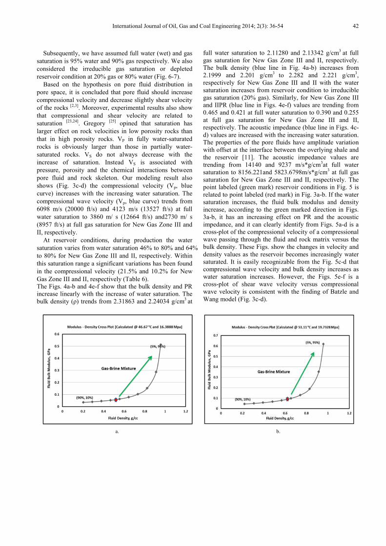
Subsequently, we have assumed full water (wet) and gas

saturation is 95% water and 90% gas respectively. We also

considered the irreducible gas saturation or depleted

reservoir condition at 20% gas or 80% water (Fig. 6-7).

Based on the hypothesis on pore fluid distribution in

pore space, it is concluded that pore fluid should increase

compressional velocity and decrease slightly shear velocity

of the rocks [2,3]

. Moreover, experimental results also show

that compressional and shear velocity are related to

saturation [23,24]

. Gregory [25]

opined that saturation has

larger effect on rock velocities in low porosity rocks than

that in high porosity rocks. VP in fully water-saturated

rocks is obviously larger than those in partially water-

saturated rocks. VS do not always decrease with the

increase of saturation. Instead VS is associated with

pressure, porosity and the chemical interactions between

pore fluid and rock skeleton. Our modeling result also

shows (Fig. 3c-d) the compressional velocity (Vp, blue

curve) increases with the increasing water saturation. The

compressional wave velocity (Vp, blue curve) trends from

6098 m/s (20000 ft/s) and 4123 m/s (13527 ft/s) at full

water saturation to 3860 m/ s (12664 ft/s) and2730 m/ s

(8957 ft/s) at full gas saturation for New Gas Zone III and

II, respectively.

At reservoir conditions, during production the water

saturation varies from water saturation 46% to 80% and 64%

to 80% for New Gas Zone III and II, respectively. Within

this saturation range a significant variations has been found

in the compressional velocity (21.5% and 10.2% for New

Gas Zone III and II, respectively (Table 6).

The Figs. 4a-b and 4e-f show that the bulk density and PR

increase linearly with the increase of water saturation. The

bulk density (ρ) trends from 2.31863 and 2.24034 g/cm3

at

full water saturation to 2.11280 and 2.13342 g/cm3

at full

gas saturation for New Gas Zone III and II, respectively.

The bulk density (blue line in Fig. 4a-b) increases from

2.1999 and 2.201 g/cm3

to 2.282 and 2.221 g/cm3,

respectively for New Gas Zone III and II with the water

saturation increases from reservoir condition to irreducible

gas saturation (20% gas). Similarly, for New Gas Zone III

and IIPR (blue line in Figs. 4e-f) values are trending from

0.465 and 0.421 at full water saturation to 0.390 and 0.255

at full gas saturation for New Gas Zone III and II,

respectively. The acoustic impedance (blue line in Figs. 4c-

d) values are increased with the increasing water saturation.

The properties of the pore fluids have amplitude variation

with offset at the interface between the overlying shale and

the reservoir [11]. The acoustic impedance values are

trending from 14140 and 9237 m/s*g/cm3at full water

saturation to 8156.221and 5823.6798m/s*g/cm3 at full gas

saturation for New Gas Zone III and II, respectively. The

point labeled (green mark) reservoir conditions in Fig. 5 is

related to point labeled (red mark) in Fig. 3a-b. If the water

saturation increases, the fluid bulk modulus and density

increase, according to the green marked direction in Figs.

3a-b, it has an increasing effect on PR and the acoustic

impedance, and it can clearly identify from Figs. 5a-d is a

cross-plot of the compressional velocity of a compressional

wave passing through the fluid and rock matrix versus the

bulk density. These Figs. show the changes in velocity and

density values as the reservoir becomes increasingly water

saturated. It is easily recognizable from the Fig. 5c-d that

compressional wave velocity and bulk density increases as

water saturation increases. However, the Figs. 5e-f is a

cross-plot of shear wave velocity versus compressional

wave velocity is consistent with the finding of Batzle and

Wang model (Fig. 3c-d).

a. b.



c. d.

Fig. 3. Cross-plot of fluid modulus and density as saturation values change (gas%, brine %) for a) New Gas Zone III and b) New Gas Zone II. Velocity

versus saturation shows how water saturation affects a two phase mixture of gas and brine in a sandstone matrix from water to gas saturated conditions for c) New Gas Zone III and d) New Gas Zone II.

a. b.

c. d.


e. f.

Fig. 4. Bulk density versus saturation for a) New Gas Zone III and b) New Gas Zone II, Acoustic Impedance versus saturation for c) New Gas Zone III

and d) New Gas Zone II, and Poisson’s ratio versus saturation for e) New Gas Zone III and f) New Gas Zone II shows how water saturation affects a two

phase mixture of gas and brine in a sandstone matrix from water to gas saturated conditions.

a. b.

c. d.



e. f.

Fig. 5. Acoustic impedance Vs. Poisson’s ratio cross-plot for a) New Gas Zone III and b) New Gas Zone II, Compressional wave velocity Vs. Bulk density

cross-plot for c) New Gas Zone III and d) New Gas Zone II, and Shear wave velocity Vs. Compressional wave velocity cross-plot for e) New Gas Zone III

and f) New Gas Zone II for a two phase mixture of gas and brine in a sandstone matrix from water to gas saturated conditions.

a. b.

c. d.

Fig. 6. Fluid modulus versus pressure shows the changes in the fluid modulus as the pressure and saturation in the reservoir changes during production

for a) New Gas Zone III and b) New Gas Zone II. Fluid density versus pressure shows the changes in the fluid density as the pressure and saturation in

the reservoir changes during production for c) New Gas Zone III and d) New Gas Zone II.


4.2. Fluid Models for Varying Saturation and Pressure

4.2.1. Batzle and Wang Model

Here we considered gas saturation would change from

90% to 10% of reservoir pressure of 2000 psi, 1500 psi and

1000 psi pressure for New Gas Zone III and at reservoir

pressure of 2500 psi, 2000 psi, 1500 psi and 1000 psi for

New Gas Zone II. The moduli and densities for different

saturation and pressure were calculated from this model are

listed (Table 7). The cross plot between fluid modulus and

density versus pressure shows that the fluids have a wide

range of fluid moduli and densities of different saturation

conditions (Fig. 6). The different fluid moduli and densities

for the initial reservoir pressure conditions are shown by

the yellow diamonds. In this line the red diamond indicates

the initial saturation point. The light brown diamond series

is for 17.236893 MPa (2500 psi), dark brown series is

for3.789514 MPa (2000 psi), blue diamond series is for

10.342136 MPa (1500 psi) and the last black diamond

series is for 6.894757 MPa (1000 psi) pressure. For New

Gas Zone III, we assumed that during production fluid

saturations (Gas: Brine) would (0.54: 0.46), (0.50: 0.50),

(0.40: 0.60) and (0.30: 0.70) at 16.38884 MPa (2377 psi),

13.789514 MPa (2000 psi), 10.342136 MPa (1500 psi) and

6.894757 MPa (1000 psi) pressure, respectively. Similarly,

for New Gas Zone II we also assumed that during

production fluid saturations (Gas: Brine) would (0.36: 0.64),

(0.32: 0.68), (0.28: 0.72), (0.24: 0.76) and (0.20: 0.80) at

19.737279 MPa (2862 psi), 17.236893 MPa (2500 psi),

13.789514 MPa (2000 psi), 10.342136 MPa (1500 psi) and

6.894757 MPa (1000 psi) pressure, respectively. The dry

frame modulus is held constant. Figs. 6a-b is showing the

predicted fluid modulus path versus pressure. The black

connecting line with arrow head shows the downward

curve for the decreasing value of fluid modulus with

respect to pressure fall during production. The fluid

modulus increases with water saturation at a constant

pressure, but decreases with pressure fall and overall it

decreases through the assumed production path. So, the

effect of pressure fall is dominating here for fluid modulus

changes.

Table 6. Calculated values of Gassmann-Biot model (for varying saturation with constant pressure).

Zo

nes Water

Saturation,

ρw

Dry Frame

Rigidity, G

Bulk

Density,

g/cm3

Fluid Bulk

Modulus, Kf

Saturated

Bulk

Modulus, Kb

P-Wave

Velocity,

Vp

S-Wave

Velocity,

Vs

Poisson’s

Ratio, σ

Acoustic

impedance,

AI

New

Gas

Zon

e II

I

0.1 5.67431 2.11280 0.03536 23.9203 3860.38 1638.80 0.39008 8156.221

0.2 5.67431 2.13701 0.03971 26.0534 3966.33 1629.49 0.39847 8476.134

0.3 5.67431 2.16123 0.04528 28.6042 4090.94 1620.34 0.40696 8841.479

0.4 5.67431 2.18544 0.05267 31.7087 4239.21 1611.33 0.41556 9264.569

0.46 5.67431 2.19997 0.05838 33.9173 4342.36 1606.00 0.42076 9553.107

0.5 5.67431 2.20966 0.06294 35.5690 4418.25 1602.48 0.42426 9762.856

0.6 5.67431 2.23387 0.07818 40.4996 4638.59 1593.77 0.43307 10362.06

0.7 5.67431 2.25809 0.10316 47.0172 4916.51 1585.20 0.44199 11101.95

0.8 5.67431 2.28230 0.15159 56.0348 5278.9 1576.77 0.45102 12048.07

0.9 5.67431 2.30652 0.28574 69.3323 5774.02 1568.47 0.46016 13317.93

0.95 5.67431 2.31863 0.51251 78.6664 6098.44 1564.37 0.46478 14140.03

New

Gas

Zon

e II

0.1 5.21752 2.13342 0.044669 8.940381 2729.727 1563.842 0.255723 5823.6798

0.2 5.21752 2.14600 0.050141 9.758707 2790.889 1559.252 0.273109 5989.2691

0.3 5.21752 2.15858 0.057142 10.74193 2863.418 1554.703 0.290983 6180.9366

0.4 5.21752 2.17116 0.066415 11.94548 2950.592 1550.192 0.309366 6406.2241

0.5 5.21752 2.18374 0.079281 13.45275 3057.135 1545.721 0.32828 6676.0001

0.6 5.21752 2.19632 0.098329 15.39533 3190.143 1541.289 0.347748 7006.5846

0.64 5.21752 2.20135 0.108784 16.33908 3253.07 1539.526 0.355696 7161.1596

0.7 5.21752 2.20890 0.129425 17.99361 3360.853 1536.894 0.367795 7423.7942

0.8 5.21752 2.22148 0.189284 21.64697 3588.306 1532.536 0.388448 7971.3515

0.9 5.21752 2.23405 0.352158 27.16182 3907.938 1528.216 0.409735 8730.5641

0.95 5.21752 2.24034 0.618079 31.12681 4122.973 1526.069 0.420624 9236.8976

However, a reverse condition has been seen from the Figs. 6c-d, which indicates that the fluid density of the reservoir is

not affected as strongly as the modulus by pressure changes and variations of saturation. The density is increasing with the

increase of water saturation and decreases with pressure fall for both gas zones.



a. b.

c. d.

e. f.

Fig. 7. P-wave velocity versus pressure shows how the velocity changes as the pressure and saturation in the reservoir changes for a) New Gas Zone III

and b) New Gas Zone II. The Poisson’s ratio versus pressure shows how the velocity changes as the pressure and saturation in the reservoir changes for c)

New Gas Zone III and d) New Gas Zone II. Acoustic impedance versus pressure shows how the Poisson’s ratio changes as the pressure and saturation in

the reservoir changes for e) New Gas Zone III and f) New Gas Zone II.

Table 7. Calculated fluid properties from Batzle and Wang Model (for varying saturation and pressure).

Calculation for New Gas Zone III

Pressure: 16.38884 Mpa (2377 psi) Pressure: 13.7895 Mpa (2000 psi)

Density of Gas: 0.115 g/cc Density of Gas: 0.0963 g/cc

Modulus of Gas: 0.031754 Gpa Modulus of Gas: 0.025795 Gpa

Density of Brine: 1.0019 g/cc Density of Brine: 1.0008 g/cc

Modulus of Brine: 2.483332 Gpa Modulus of Brine: 2.466893 Gpa

Gas % Brine % Density, g/cc Modulus, Gpa Gas % Brine % Density, g/cc Modulus, Gpa

90 10 0.2038 0.035367 90 10 0.1868 0.028627

80 20 0.2924 0.039717 80 20 0.2772 0.032159

70 30 0.3811 0.045287 70 30 0.3677 0.036685



60 40 0.4698 0.052675 60 40 0.4581 0.042693

54 46 0.523 0.05839 50 50 0.5486 0.051055

50 50 0.5585 0.062943 40 60 0.639 0.063491

40 60 0.6472 0.078183 30 70 0.7295 0.083934

30 70 0.7359 0.103162 20 80 0.8199 0.123795

20 80 0.8246 0.151594 10 90 0.9104 0.235759

10 90 0.9132 0.285744

Pressure: 10.3421 Mpa (1500 psi) Pressure: 6.8948 Mpa (1000 psi)






90 10 0.1636 0.020384 90 10 0.1407 0.012756

80 20 0.2563 0.022909 80 20 0.2359 0.014341

70 30 0.3493 0.026146 70 30 0.3312 0.016375

60 40 0.4422 0.030449 60 40 0.4264 0.019083

50 50 0.5351 0.036449 50 50 0.5217 0.022864

40 60 0.6279 0.045392 40 60 0.6169 0.028512

30 70 0.7208 0.06015 30 70 0.7122 0.037868

20 80 0.8137 0.089129 20 80 0.8075 0.056362

10 90 0.9065 0.171989 10 90 0.9027 0.110163

Calculation for New Gas Zone II

Pressure: 19.73279 Mpa (2862 psi) Pressure: 17.236893 Mpa(2500 psi)

Density of Gas: 0.1346 g/c Density of Gas: 0.1182 g/cc





90 10 0.2214 0.044669 90 10 0.2065 0.037621

80 20 0.3081 0.050141 80 20 0.2948 0.042244

70 30 0.3949 0.057142 70 30 0.3831 0.048163

60 40 0.4817 0.066415 60 40 0.4714 0.056011

50 50 0.5684 0.079281 50 50 0.5597 0.066915

40 60 0.6552 0.098329 40 60 0.6479 0.083089

36 64 0.6899 0.108783 30 70 0.7363 0.109574

30 70 0.7419 0.129424 20 80 0.8246 0.160846

20 80 0.8286 0.189281 10 90 0.9129 0.302297

10 90 0.9154 0.352146

Pressure: 13.789514 Mpa(2000 psi) Pressure: 10.342136 Mpa(1500 psi)






90 10 0.1847 0.022868 90 10 0.1621 0.020469

80 20 0.2752 0.032219 80 20 0.255 0.023004

70 30 0.3658 0.036764 70 30 0.3479 0.026255

60 40 0.4564 0.042774 60 40 0.4408 0.030576

50 50 0.5469 0.051153 50 50 0.5338 0.036601

40 60 0.6375 0.063614 40 60 0.6267 0.045582

30 70 0.7281 0.084101 30 70 0.7196 0.060403

20 80 0.8186 0.124052 20 80 0.8125 0.089507

10 90 0.9092 0.236305 10 90 0.9054 0.172735

Pressure: 6.894757 Mpa(1000 psi)

Density of Gas: 0.0445 g/cc Density of Brine: 0.9969 g/cc

Modulus of Gas: 0.011539 Gpa Modulus of Brine: 2.440969 Gpa

Gas % Brine % Density, g/cc Modulus, Gpa

90 10 0.1397 0.012815

80 20 0.2349 0.014408

70 30 0.3302 0.016452

60 40 0.4255 0.019172

50 50 0.5207 0.022971

40 60 0.6159 0.028646

30 70 0.7112 0.038046

20 80 0.8064 0.056628

10 90 0.9017 0.110688



4.2.2.Gassmann-Biot Model

The initial conditions of the Figs. are same as the Fig. 6.

Biot-Gassmann theory accurately predicts velocity ratios

with respect to differential pressure for given porosity.

However, because the velocity ratio is weakly related to

porosity, it is not appropriate to investigate the velocity

ratio with respect to porosity (φ). The velocity ratio has

been used for many purposes, such as a lithology indicator,

determining degree of consolidation, identifying pore fluid,

and predicting velocities [27]

. The velocity ratio usually

depends on porosity, degree of consolidation, clay content,

differential pressure, pore geometry, and other factors. The

velocity ratio for dry rock or gas-saturated rock is almost a

constant irrespective of porosity and differential pressure,

whereas the velocity ratio of wet rock depends significantly

on porosity and differential pressure. P-wave to S-wave

velocity ratio (Vp/V

s) for the both gas zones Fenchuganj

Gas Field show value of more than 2.0 which indicate the

presence of gas in the unconsolidated rock [28]

with higher

porosity [29]

.

Fig. 7 shows the predicted P-wave velocity, PR and

acoustic impedances under differential pressure due to gas

production increases. The black connecting line with arrow

head shows the downward curve for the decreasing value of

all parameters respects to pressure fall during production.

These parameters increases with water saturation at a

constant pressure, but decreases with pressure fall. So, it

can forecast that the New Gas Zone II has greater effect on

parameters change than the New Gas Zone III.

4.3. AVO Analysis

In this section, we determined and analyzed the AVO

response for New Gas Zone III and II of Fenchuganj Gas

Field. Firstly, we took assumptions given by Shuey [21]

(1985) and interpreted AVO using Zoeppritz (1919)

equation for 0-30° incident angle.

a. b.

c. d.

Fig. 8. Reflection amplitude versus offset shows the AVO between a definite pressure-saturation condition and reservoir condition for a) New Gas Zone

III and b) New Gas Zone II. Reflection amplitude versus offset shows the AVO between a) New Gas Zone III and above shale zone, and b) New Gas Zone

II and above shale zone.

The input values (Vp, ρb and σ) for AVO interpretation

are taken from the output values (Table 8) of Gassmann-

Biot model for varying saturation and pressure. Every

reflection curve of Figs. 8a-b represents the comparison of

seismic reflection change due to change of pressure and

saturation of a definite layer from the reservoir condition. It

is obvious that the AVO response decreases as water

saturation increases.

Secondly, we have interpreted AVO without any

assumptions. We used full Zoeppritz [1] equation with the

help of an AVO calculator by Timothy et al. which starts

with negative values and decreases with the offset


indicating of low impedance gas sand class 3 AVO [11]

.

This characteristic of AVO indicates bright zone that is

potential for hydrocarbon zone [11]

.

Table 8. Calculated fluid and rock properties from Gassmann-Biot Model (for varying saturation and pressure).


Input Parameters (Fixed) Symbol Value Unit

Depth D 1656-1680 m

Temperature T 46.67 °C

Solid Material Bulk Modulus Ks 30 Gpa

Solid Material Density ρs 2.8297 g/cc

Logged P-wave velocity Vpi 2650 m/s

Logged S-wave velocity Vsi 1606 m/s

Logged Bulk Density ρbi 2.2 g/cc

Fluid Bulk Modulus at logged condition Kfi 0.5839 Gpa

Parameter (Variable) Symbol Value Unit

Pressure P 16.3884 Mpa

Water Bulk Modulus Kw 2.483332 GPa

Water Density ρw 1.0019 g/cc

Hydrocarbon Bulk Modulus Khyd 0.031754 Gpa

Hydrocarbon Density ρhyd 0.115 g/cc

Sw Sg ρb in g/cc Vp in m/s Vs in m/s σ AI

0.1 0.9 2.11279927 3860.397409 1638.80682 0.39008381 8156.24483

0.2 0.8 2.13701164 3966.357727 1629.49652 0.39847393 8476.15263

0.3 0.7 2.16122401 4090.965635 1620.34312 0.40696595 8841.49315

0.4 0.6 2.18543638 4239.234444 1611.34226 0.41556172 9264.57718

0.46 0.54 2.1999638 4342.39474 1606.01321 0.42076978 9553.11124

0.5 0.5 2.20964875 4418.284777 1602.48975 0.42426317 9762.85743

0.6 0.4 2.23386112 4638.628155 1593.78156 0.43307226 10362.0511

0.7 0.3 2.25807349 4916.552911 1585.2138 0.44199099 11101.9378

0.8 0.2 2.28228586 5278.937105 1576.78276 0.45102143 12048.0435

0.9 0.1 2.30649823 5774.067549 1568.48482 0.46016568 13317.8766





Hydrocarbon Balk Modulus K hyd 0.025795 Gpa

Hydrocarbon Density ρ hyd 0.0963 g/cc


0.1 0.9 2.10817465 3638.34716 1640.60333 0.37238851 7670.27125

0.2 0.8 2.1328675 3739.577122 1631.0788 0.38253207 7976.02251

0.3 0.7 2.15756035 3860.010094 1621.71825 0.3928267 8328.20473

0.4 0.6 2.1822532 4005.19392 1612.51704 0.40327579 8740.34725

0.5 0.5 2.20694605 4183.197791 1603.47068 0.41388284 9232.09184

0.6 0.4 2.2316389 4406.28949 1594.57489 0.42465147 9833.24703

0.7 0.3 2.25633175 4694.207908 1585.82553 0.43558538 10591.6903

0.8 0.2 2.2810246 5081.196991 1577.21862 0.44668843 11590.3353

0.9 0.1 2.30571745 5633.260806 1568.75036 0.45796456 12988.7077








0.1 0.9 2.10184651 3308.279078 1643.0712 0.33628418 6953.49483

0.2 0.8 2.12720002 3398.769408 1633.25019 0.34987236 7229.86235

0.3 0.7 2.15255353 3508.428829 1623.60321 0.36373972 7552.08086

0.4 0.6 2.17790704 3643.361622 1614.12518 0.37789496 7934.90293

0.5 0.5 2.20326055 3812.755286 1604.81122 0.39234714 8400.49331

0.6 0.4 2.22861406 4031.192373 1595.65666 0.40710569 8983.972




0.7 0.3 2.25396757 4323.493664 1586.65699 0.42218046 9745.01451

0.8 0.2 2.27932108 4736.177418 1577.80791 0.43758173 10795.269

0.9 0.1 2.30467459 5369.75109 1569.10525 0.45332021 12375.5289








0.1 0.9 2.09558935 2918.85671 1645.52237 0.26705498 6116.72504

0.2 0.8 2.1215926 2990.866675 1635.40712 0.28674271 6345.40061

0.3 0.7 2.14759585 3080.425548 1625.47616 0.30705192 6615.50912

0.4 0.6 2.1735991 3193.738128 1615.72393 0.32801249 6941.90632

0.5 0.5 2.19960235 3340.516514 1606.14516 0.34965628 7347.80797

0.6 0.4 2.2256056 3536.966232 1596.73476 0.37201725 7871.89185

0.7 0.3 2.25160885 3812.576793 1587.48784 0.39513164 8584.43165

0.8 0.2 2.2776121 4228.152764 1578.39974 0.41903818 9630.0919

0.9 0.1 2.30361535 4936.554275 1569.46596 0.44377831 11371.9222

Calculation for New Gas Zone II

Input Parameters (Fixed) Symbol Value Unit

Depth D 1992-2017 m

Temperature T 51.11 °C

Solid Material Bulk Modulus Ks 30 Gpa

Solid Material Density ρs 2.4577 g/cc

Logged P-wave velosity Vpi 2540 m/s

Logged S-wave velosity Vsi 1540 m/s

Logged Bulk Density ρ bi 2.2 g/cc

Fluid Bulk Modulus at logged condition K fi 1.0878 Gpa





Hydrocarbon Bulk Modulus K hyd 0.040273 Gpa



0.1 0.9 2.1334307 2729.725935 1563.84171 0.25572341 5823.68111

0.2 0.8 2.1460109 2790.885916 1559.25125 0.27310896 5989.2716

0.3 0.7 2.1585911 2863.414022 1554.70097 0.29098267 6180.94002

0.4 0.6 2.1711713 2950.586243 1550.19031 0.30936539 6406.22817

0.5 0.5 2.1837515 3057.12635 1545.71867 0.32827919 6676.00425

0.6 0.4 2.1963317 3190.131988 1541.28551 0.3477474 7006.58801

0.64 0.36 2.20136378 3253.057256 1539.5229 0.35569542 7161.16242

0.7 0.3 2.2089119 3360.838207 1536.89028 0.36779478 7423.79551

0.8 0.2 2.2214921 3588.285493 1532.53243 0.38844756 7971.34788

0.9 0.1 2.2340723 3907.908371 1528.21145 0.40973358 8730.54984








0.1 0.9 2.131276 2632.695017 1564.63202 0.22696096 5610.99971

0.2 0.8 2.1440795 2690.39877 1559.95338 0.24676791 5768.42885

0.3 0.7 2.156883 2759.534441 1555.31646 0.26722484 5951.99292

0.4 0.6 2.1696865 2843.596333 1550.72064 0.28836427 6169.71257

0.5 0.5 2.18249 2947.723805 1546.16533 0.31022094 6433.37773

0.6 0.4 2.1952935 3079.830248 1541.64992 0.33283198 6761.13133



0.7 0.3 2.208097 3252.839175 1537.17385 0.35623714 7182.58442

0.8 0.2 2.2209005 3489.581914 1532.73654 0.38047899 7750.01422

0.9 0.1 2.233704 3835.119202 1528.33743 0.40560321 8566.5211








0.1 0.9 2.12811065 2492.057085 1565.7952 0.17385562 5303.37322

0.2 0.8 2.1412433 2543.324617 1560.98616 0.1978193 5445.8768

0.3 0.7 2.15437595 2605.74497 1556.22116 0.22278176 5613.7543

0.4 0.6 2.1675086 2683.017631 1551.49952 0.24880679 5815.46379

0.5 0.5 2.18064125 2780.743464 1546.82061 0.2759637 6063.8039

0.6 0.4 2.1937739 2907.86359 1542.18377 0.30432798 6379.19525

0.7 0.3 2.20690655 3079.678977 1537.58838 0.33398196 6796.56371

0.8 0.2 2.2200392 3324.999405 1533.03383 0.36501567 7381.62902

0.9 0.1 2.23317185 3706.263383 1528.51952 0.39752769 8276.72305








0.1 0.9 2.12483945 2340.677718 1567.00002 0.09390356 4973.56435

0.2 0.8 2.1383114 2383.083886 1562.05595 0.12334578 5095.77544

0.3 0.7 2.15178335 2435.760627 1557.15839 0.15441668 5241.22916

0.4 0.6 2.1652553 2502.416377 1552.30661 0.18725524 5418.37032

0.5 0.5 2.17872725 2588.847254 1547.4999 0.22201673 5640.39206

0.6 0.4 2.1921992 2704.685366 1542.73756 0.25887514 5929.2091

0.7 0.3 2.20567115 2867.309349 1538.01893 0.29802612 6324.34151

0.8 0.2 2.2191431 3111.956128 1533.34333 0.33969042 6905.87597

0.9 0.1 2.23261505 3524.244468 1528.71011 0.38411808 7868.28124








0.1 0.9 2.1215958 2174.203564 1568.19743 -0.0421808 4612.78115

0.2 0.8 2.1354056 2204.4346 1563.11839 -0.0056176 4707.36199

0.3 0.7 2.1492154 2243.112284 1558.08838 0.03384788 4820.93146

0.4 0.6 2.1630252 2293.580296 1553.10662 0.0765754 4961.07198

0.5 0.5 2.176835 2361.261639 1548.17235 0.12298686 5140.07698

0.6 0.4 2.1906448 2455.603094 1543.2848 0.17358016 5379.35415

0.7 0.3 2.2044546 2594.756297 1538.44325 0.22894717 5720.02245

0.8 0.2 2.2182644 2819.013639 1533.64699 0.28979696 6253.3176

0.9 0.1 2.2320742 3241.896491 1528.89531 0.35698639 7236.15352

Table 9. The inputs for Shale zones above gas layer and Gas zones for determining AVO.

Above Shale Zone/Gas Zone P-Velocity (Vp) S-Velocity (Vs) Bulk Density (ρb)

g/cm3 m/sec ft/sec m/sec ft/sec

Shale Zone Above New gas Zone III 4000 13123 2116 6942 2.40

Shale Zone Above New gas Zone II 3800 12467 2011 6598 2.40

New gas Zone III 2650 8694 1606 5269 2.20

New gas Zone II 2540 8333 1540 5053 2.20



5. Conclusion

The Batzle and Wang model has predicted the fluid

properties for both of the constant/varying saturation with

constant/varying pressure condition that are near accurate

forecasting. Increase of water saturation effects on fluid

properties by increasing the fluid density, modulus and

acoustic velocity. However, the compressibility of fluid

decreases as the water in fluid increases. As temperature

increases, the velocity and density of the fluid decrease.

The cross plots using the Batzle and Wang model on

densities and moduli allows to predict the fluid properties

as the reservoir is produced and shows the effect on the

reservoir as water saturation increases and gas saturation

decreases. The change in P-wave and S- wave velocity,

bulk density, acoustic impedance, Poisson’s ratio, and bulk

modulus were predicted using the Batzle and Wang and

Gassmann-Biot model. The result shows that the reservoir

changes from irreducible water saturation conditions in

residual gas conditions which provide an avenue to

calculate values at reservoir conditions from logging

conditions. Coupling with the Batzle and Wang (1995),

Gassmann-Biot, the AVO models can be used to determine

expected seismic responses throughout the production path

of the reservoir. In case of the Fenchuganj Gas Field, it is

shown that an AVO response is presented as a result of the

fluid and rock properties. This modeling results show the

reservoir is pressure decreases due to increasing the gas

production. The evaluation of fluid properties enables

seismic data to be used more effectively. This modeling

fluid property will aid in determining the usefulness of time

lapse seismic, predicting AVO and amplitude response, and

making production and reservoir engineering decisions and

forecasting.

Acknowledgment

The authors are grateful to BAPEX authority, especially

Geological and Geophysical Division for allowing

collecting the necessary data and use their software for this

work. The first author is also grateful to Mr. Md. Shofiqul

Islam, Geology Division (BAPEX) and Mr. Pulok Kanti

Deb, Department of Petroleum and Mining Engineering,

Shahjalal University for their help and suggestions to

improve this work.

References

[1] Zoeppritz, K., 1919, Erdbebenwellen VIIIB, On the reflection and propagation of seismic waves, Gottinger Nachrichten, I, p. 66-84.

[2] Gassmann, F., 1951, Elastic waves through a packing of spheres: Geophysics, 16, 673-685.

[3] Biot, M. A., 1956, Theory of propagation of elastic waves in a fluid-saturated porous solid: Journal of Acoustical Society of America, 28, 168-191.

[4] Kuster, G.T., and Toksöz, M.N., 1974, Velocity and attenuation of seismic waves in two-phase media: Part I. theoretical formulations: Geophysics, 39, 587-606.

[5] O'Connell R., Budiansky B. 1974, Seismic velocities in dry and saturated crack solids. Journal of geophysical Research, 79, 5412-5426.

[6] Rutherford, S.R. and Williams, R.H., 1989, Amplitude-versus-offset variations in gas sands: Geophysics, 54, 680-688.

[7] Mavko, G., and Jizba, D. 1991, Estimating grain-scale fluid effects on velocity dispersion in rocks, Geophysics, 56(12), 1940–1949, doi:10.1190/1.1443005.

[8] Batzle, M. and Wang, Z., 1992, Seismic properties of pore fluids: Geophysics, Vol. 57(11), 1396-1408.

[9] Sheriff, R.E., 1991, Encyclopedic Dictionary of Exploration Geophysics, 3rd Edition: SEG Geophysical References Series 1, Tulsa, USA, p. 384.

[10] Castagna, J.P. and Swan, H.W., 1997, Principles of AVO crossplotting: The Leading Edge, 16, 337-342.

[11] Bulloch, T.E., 1999, The Investigation Of Fluid Properties And Seismic Attributes For Reservoir Characterization, M.Sc thesis for Geological Engineering, Michigan TechnologicaI University, USA.

[12] Annual Report, 2010, Bangladesh Petroleum Exploration and Production Company Limited (BAPEX), Bangladesh

[13] Mannan, M. A., 2002, Stratigraphic evolution and geochemistry of the Neogene Surma Group, Surma Basin, Sylhet, Bangladesh, PhD Dissertation, Department of Geology, University of Oulu.

[14] Farhaduzzaman, M., Wan Hasiah A., Islam, M. A., and Pearson, M. J., 2012, Source rock potential of the organic-rich shales in the Tertiary Bhuban and BokaBil Formations, Bengal Basin, Bangladesh. Journal of Petroleum Geology, 35 (4), 357-376.

[15] Sheriff, R.E., and Geldart, L.P., 1995, Exploration Seismology, 2nd Edition: Cambridge University Press, New York, USA, p. 592.

[16] Murphy, W.F., Schwartz, L.M., and Hornby, B., 1991, Interpretation physics of Vp and Vs in sedimentary rocks: Transactions SPWLA 32nd Annual Logging Symp., p. 1-24.

[17] Schlumberger Oilfield Glossary. (URL: http://www.glossary.oilfield.slb.com/en/Terms.aspx?LookIn=term%20name&filter=amplitude%20variation%20with%20offset)

[18] Mavko, G., Mukerji, T., Dvorkin, J., 1998, The Rock Physics Handbook: Tools for Seismic Analysis in Porous Media: Cambridge University Press, Cambridge, New York, USA, 329 pp.

[19] Castagna, J. P., and Backus, M. M., 1993, Offset-Dependent Reflectivity -Theory and Practice of AVO Analysis: SEG Investigations in Geophysics Series, 8, Tulsa, USA, 348.


[20] Hales, A.L., and Roberts, J.L., 1974, The Zoeppritz amplitude equations: more errors: Bulletin of Seismological Society of America, Vol. 64, p. 285.

[21] Aki, K., and Richards, P.G., 1980, Quantitative seismology: Theory and methods: W. H. Freeman and Co.

[22] Shuey, R.T., 1985, A simplification of the Zoeppritz equations: Geophysics, 50, 609-614

[23] Hilterman, F., 1989, Is AVO the seismic signature of rock properties? 59th Ann. Internat. Mtg., Soc. Expl. Geophys., Expanded Abstracts, 559.

[24] Knigh R, Nolen-Hoeksema R. A., 1990, laboratory study of the dependence of elastic wave velocities on pore scale fluid distribution. Geophysical Research Letters, 17 (10), 1529-1532.

[25] Liu Zhupin, WU Xiaowei, Chu Zehan 1994, Laboratory study of acoustic parameters of rock. Chinese Journal of Geophysics (Acta Geophysica Sinica), 37 (5): 659-666.

[26] Gregory A R. Fluid saturation on dynamic elastic properties of sedimentary rocks. Geophysics, 1976, 41 (5), 895-921.

[27] Lee, M.W., 2003, Elastic Properties of Overpressured and Unconsolidated Sediments, U.S. Geological Survey Bulletin 2214, Version 1.0, 1-10.

[28] Gardner, G. H. F. and Harris, M.H., 1968, Velocity and attenuation of elastic waves in sands: Society of Professional Well Log Analysts, Transactions, 9th Annual Log Symposium, p. M1–M19.

[29] Pickett, G.R., 1963, Acoustic character logs and their applications in formation evaluation: Journal of Petroleum Technology, 15, 650–667.

[30] Deb, P. K., 2011, An application of seismic and well log

techniques to the structural and stratigraphic development of

Fenchuganj Gas Field, B.Sc thesis, Department of

Petroleum and Mining Engineering, SUST, Bangladesh.

Investigation of fluid properties and their effect on seismic...

Documents

Transcript of Investigation of fluid properties and their effect on seismic...