Investigation of Factors Related to Surface-Initiated ... OF FACTORS RELATED TO SURFACE-INITIATED...
191
2003-07 Final Report Investigation of Factors Related to Surface-Initiated Cracks in Flexible Pavements Minnesota Local Road Research Board
Transcript of Investigation of Factors Related to Surface-Initiated ... OF FACTORS RELATED TO SURFACE-INITIATED...

2003-07
Final Report
Investigation of Factors Related to Surface-Initiated Cracks in Flexible
Pavements
Minnesota LocalRoad ResearchBoard

Technical Report Documentation Page 1. Report No. 2. 3. Recipients Accession No. MN/RC - 2003-07 4. Title and Subtitle 5. Report Date
January 2003 6.
INVESTIGATION OF FACTORS RELATED TO SURFACE-INITIATED CRACKS IN FLEXIBLE PAVEMENTS
7. Author(s) 8. Performing Organization Report No. Jill M. Holewinski, See-Chew Soon, Andrew Drescher, and Henryk Stolarski
9. Performing Organization Name and Address 10. Project/Task/Work Unit No. 11. Contract (C) or Grant (G) No.
Department of Civil Engineering University of Minnesota 500 Pillsbury Drive S.E., Minneapolis, MN 55455-0220 (c) 74708 (w)181
12. Sponsoring Organization Name and Address 13. Type of Report and Period Covered
Final Report 2001-2003 14. Sponsoring Agency Code
Minnesota Department of Transportation 395 John Ireland Boulevard Mail Stop 330 St. Paul, Minnesota 55155 15. Supplementary Notes 16. Abstract (Limit: 200 words) This report has two distinctive, yet related objectives: 1) identifying potential mechanisms for the occurrence of top-down cracking and 2) investigating stress patterns and stress concentrations due to surface load and preexisting transverse (thermal) cracks in flexible pavement. Analytic and numerical studies of multilayer elastic systems subject to wheel loads has linked longitudinal cracking to surface tensile stresses. However, due to the complexity of tire/pavement interaction resulting from tire geometry and loading conditions, the accurate and fully representative distribution of surface stresses remains partly unknown. The majority of flexible pavements experience thermal or transverse cracking in Minnesota. The presence of a transverse crack in the AC layer represents a discontinuity, which violates the assumption of unlimited pavement extent made in the theoretical, predominantly elastic solutions for the stresses and strains. The report attempts to provide information on surface stresses. In particular, contact mechanics solutions are analyzed to gain information on loads that are subsequently used in performing numerical evaluation of surface stresses using ABAQUS. The results indicate a greater potential for tensile stresses outside the tire treads than in the middle of treads. This report describes the results of three-dimensional numerical computations using ABAQUS to evaluate stresses in flexible pavement systems with a transverse crack present. It was observed that the presence of a transverse crack significantly increase the vertical stresses in the base. It also has a noticeable effect on the horizontal stresses in the AC layer.
17. Document Analysis/Descriptors 18. Availability Statement Longitudinal cracks Transverse cracks Flexible pavements
ABAQUS finite element analysis
No restrictions. Document available from National Technical Information Services, Springfield, Virginia 22161
19. Security Class (this report) 20. Security Class (this page) 21. No. of Pages 22. Price Unclassified Unclassified 191

INVESTIGATION OF FACTORS RELATED TO SURFACE-INITIATED CRACKS IN FLEXIBLE
PAVEMENTS
Final Report
Prepared by
Jill M. Holewinski, See-Chew Soon, Andrew Drescher, and Henryk K. Stolarski
University of Minnesota Department of Civil Engineering
122 CivE Building 500 Pillsbury Dr. S.E.
Minneapolis, MN 55455-0220
January 2003
Published by
Minnesota Department of Transportation Office of Research Services 395 John Ireland Boulevard
Mail Stop 330 St. Paul, Minnesota 55155
The contents of this report reflect the views of the authors who are responsible for the facts and
accuracy of the data presented herein. The contents do not necessarily reflect the views or policies of the Minnesota Department of Transportation at the time of publication. This report
does not constitute a standard, specification, or regulation

Table of Contents
Executive Summary ......................................................................................................................... i
CHAPTER 1 - Introduction ............................................................................................................ 1
CHAPTER 2 - Literature Review................................................................................................... 3
2.1 Introduction ........................................................................................................................... 3
2.2 Field observations of longitudinal cracks.............................................................................. 3
2.3 Experimental results for tire/pavement interfacial stresses ................................................... 4
2.4 Tire/pavement interaction models ......................................................................................... 5
CHAPTER 3 – Tire Pavement Interfacial Stresses....................................................................... 11
3.1 Modeling tire/pavement interaction..................................................................................... 11
3.2 Fundamental concepts of contact mechanics....................................................................... 11
CHAPTER 4 – Analytical Solutions............................................................................................. 15
4.1 Vertical strip load ................................................................................................................ 15
4.2 Horizontal strip load ............................................................................................................ 18
4.3 Vertical area load................................................................................................................. 20
iii

4.4 Circular horizontal load ....................................................................................................... 23
4.5 Summary of observations .................................................................................................... 24
CHAPTER 5 – Numerical Model ................................................................................................. 27
5.1 Introduction ......................................................................................................................... 27
5.2 Modeling the pavement structure – longitudinal cracking .................................................. 27
5.2.1 Modeling tire/pavement interaction .............................................................................. 27
5.2.2 Multilayer pavement system ......................................................................................... 29
5.2.3 Finite-element mesh ...................................................................................................... 30
5.2.4 Loading configuration ................................................................................................... 31
5.2.5 Material parameters....................................................................................................... 32
5.3 Modeling the pavement structure – transverse cracks......................................................... 33
5.3.1 Layered system.............................................................................................................. 33
5.3.2 Mesh .............................................................................................................................. 34
5.3.3 Material properties ........................................................................................................ 36
5.3.4 Critical stress locations and loading.............................................................................. 38
CHAPTER 6 - Numerical Results ................................................................................................ 43
6.1 Longitudinal cracks ............................................................................................................. 43
6.1.1 Surface stresses due to unit tractions............................................................................. 43
6.1.2 Surface stresses induced by tires................................................................................... 47
6.1.3 Influence of AC layer thickness .................................................................................... 52
iv

6.2 Transverse cracks ................................................................................................................ 53
6.2.1 Introduction ................................................................................................................... 53
6.2.2 Stress distributions ........................................................................................................ 54
6.2.3 Summary cross sections ................................................................................................ 63
6.2.4 Influence of material properties .................................................................................... 63
6.2.5 Influence of AC layer thickness .................................................................................... 74
6.2.6 CNR line graphs ............................................................................................................ 79
6.2.7 Surface stress related to top-down cracking.................................................................. 92
Chapter 7: Closing Remarks and Conclusions.............................................................................. 99
7.1 Surface stresses in pavement structures............................................................................... 99
7.1.1 Conclusions derived from contact mechanics .................................................................. 99
7.1.2 Conclusions derived from numerical simulations......................................................... 99
7.1.3 Remarks....................................................................................................................... 100
7.2 Influence of transverse cracking on stresses in pavement structures ................................ 101
7.2.1 Conclusions .................................................................................................................... 101
7.2.2 Remarks....................................................................................................................... 102
References................................................................................................................................... 103
Appendix C –Summary cross sections...............................................................................................C-1
v

List of Figures
FIGURE 3.1 Surface tractions acting on a stiff solid in contact problems: (a) continuous profile
R = Lc/Ls = 1; (b) continuous profile R = Lc/Ls ≈ 1 and (c) discontinuous profile R = Lc/Ls
≈ 1.......................................................................................................................................... 13
FIGURE 4.1 Flamant’s problem................................................................................................... 16
FIGURE 4.2 Uniform vertical strip load ...................................................................................... 16
FIGURE 4.3 Stresses at singular point ......................................................................................... 17
FIGURE 4.4 Horizontal normal stresses due to uniform vertical strip load................................. 17
FIGURE 4.5 Uniform horizontal strip load .................................................................................. 18
FIGURE 4.6 Horizontal normal stresses due to uniform horizontal strip load ............................ 19
FIGURE 4.7 Horizontal normal stresses due to triangular horizontal load.................................. 20
FIGURE 4.8 Boussinesq’s problem.............................................................................................. 21
FIGURE 4.9 Uniform vertical circular load ................................................................................. 22
FIGURE 4.10 Horizontal normal stresses due to uniform vertical load on circular region ......... 22
FIGURE 4.11 Uniform horizontal circular load ........................................................................... 23
FIGURE 4.12 Horizontal normal stresses due to uniform tangential load on circular region...... 24
FIGURE 4.13 Horizontal surface stresses σxx due to (a) antisymmetric tangential tractions; (b)
uni-directional tangential tractions and (c) normal tractions ................................................. 26
vii

FIGURE 5.1 Schematic reproduction of tractions applied to pavement obtained by Pottinger and
McIntyre: (a) truck tire, normal tractions; (b) passenger performance tire, normal tractions;
(c) truck tire, tangential tractions and (d) passenger performance tire, tangential tractions .. 29
FIGURE 5.2 Pavement structure .................................................................................................. 30
FIGURE 5.3 Finite element mesh................................................................................................. 31
FIGURE 5.4 Loading Configuration ............................................................................................ 32
FIGURE 5.5 Partitioned pavement structure model in ABAQUS ............................................... 35
FIGURE 5.6 Mesh ....................................................................................................................... 36
FIGURE 5.7 Horizontal tensile stresses at the bottom of the AC layer below the center of loading
................................................................................................................................................ 39
FIGURE 5.8 Vertical normal stresses in the base below the center of loading and below the edge
of the transverse crack............................................................................................................ 40
FIGURE 5.9 Shear tractions distribution for truck tire (after Pottinger and McIntyre) ............... 41
FIGURE 6.1 Influence of AC layer thickness on surface stresses σxx due to uniform normal
stresses.................................................................................................................................... 44
FIGURE 6.2 Influence of AC layer thickness on surface stresses σxx due to antisymmetric,
outward shear stresses ............................................................................................................ 45
FIGURE 6.3 Influence of AC layer thickness on surface stresses σxx due to uni-directional shear
stresses.................................................................................................................................... 46
FIGURE 6.4 Surface stresses σxx for truck tire: (a) central tread,and (b) outermost tread........... 48
FIGURE 6.5 Surface stresses σxx for passenger tire: (a) central tread and (b) outermost tread ... 49
FIGURE 6.6 Surface stresses σxx along truck tire width .............................................................. 50
viii

FIGURE 6.7 Surface stresses σxx along passenger tire width....................................................... 51
FIGURE 6.8 Variation of horizontal normal surface stresses σxx................................................. 52
FIGURE 6.9 Variation of maximum horizontal normal surface stress σxx................................... 53
FIGURE 6.10 Horizontal stresses along top of AC layer for AC = 0.1 m (Case 3): (a) stress σyy –
perpendicular to crack and (b) stress σxx – parallel to crack................................................... 55
FIGURE 6.11 Horizontal stresses along bottom of AC layer for AC = 0.1 m (Case 3): (a) stress
σyy – perpendicular to crack and (b) stress σxx – parallel to crack ......................................... 56
FIGURE 6.12 Horizontal stresses along top of AC layer for AC = 0.1 m (Case 5): (a) stress σyy –
perpendicular to crack and (b) stress σxx – parallel to crack................................................... 57
FIGURE 6.13 Horizontal stresses along bottom of AC layer for AC = 0.1 m (Case 5): (a) stress
σyy – perpendicular to crack and (b) stress σxx – parallel to crack ......................................... 58
FIGURE 6.14 Horizontal stresses along top of AC layer for AC = 0.3 m (Case 13): (a) stress σyy
– perpendicular to crack and (b) stress σxx – parallel to crack................................................ 59
FIGURE 6.15 Horizontal stresses along bottom of AC layer for AC = 0.3 m (Case 13): (a) stress
σyy – perpendicular to crack and (b) stress σxx – parallel to crack ......................................... 60
FIGURE 6.16 Horizontal stresses along top of AC layer for AC = 0.3 m (Case 15): (a) stress σyy
– perpendicular to crack and (b) stress σxx – parallel to crack................................................ 61
FIGURE 6.17 Horizontal stresses along bottom of AC layer for AC = 0.3 m (Case 15): (a) stress
σyy – perpendicular to crack and (b) stress σxx – parallel to crack ......................................... 62
FIGURE 6.18 Summary cross section for case 3, AC = 0.1 m, base = 0.076 m, and sand
subgrade = 1.42 m (C – stress in cracked pavement, NC – stress in pavement with no crack,
CNR – crack/no crack (stress) ratio) ...................................................................................... 65
ix
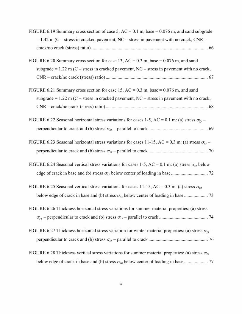
FIGURE 6.19 Summary cross section of case 5, AC = 0.1 m, base = 0.076 m, and sand subgrade
= 1.42 m (C – stress in cracked pavement, NC – stress in pavement with no crack, CNR –
crack/no crack (stress) ratio) .................................................................................................. 66
FIGURE 6.20 Summary cross section for case 13, AC = 0.3 m, base = 0.076 m, and sand
subgrade = 1.22 m (C – stress in cracked pavement, NC – stress in pavement with no crack,
CNR – crack/no crack (stress) ratio) ...................................................................................... 67
FIGURE 6.21 Summary cross section for case 15, AC = 0.3 m, base = 0.076 m, and sand
subgrade = 1.22 m (C – stress in cracked pavement, NC – stress in pavement with no crack,
CNR – crack/no crack (stress) ratio) ...................................................................................... 68
FIGURE 6.22 Seasonal horizontal stress variations for cases 1-5, AC = 0.1 m: (a) stress σyy –
perpendicular to crack and (b) stress σxx – parallel to crack .................................................. 69
FIGURE 6.23 Seasonal horizontal stress variations for cases 11-15, AC = 0.3 m: (a) stress σyy –
perpendicular to crack and (b) stress σxx – parallel to crack .................................................. 70
FIGURE 6.24 Seasonal vertical stress variations for cases 1-5, AC = 0.1 m: (a) stress σzz below
edge of crack in base and (b) stress σzz below center of loading in base............................... 72
FIGURE 6.25 Seasonal vertical stress variations for cases 11-15, AC = 0.3 m: (a) stress σzz
below edge of crack in base and (b) stress σzz below center of loading in base .................... 73
FIGURE 6.26 Thickness horizontal stress variations for summer material properties: (a) stress
σyy – perpendicular to crack and (b) stress σxx – parallel to crack ......................................... 74
FIGURE 6.27 Thickness horizontal stress variation for winter material properties: (a) stress σyy –
perpendicular to crack and (b) stress σxx – parallel to crack .................................................. 76
FIGURE 6.28 Thickness vertical stress variations for summer material properties: (a) stress σzz
below edge of crack in base and (b) stress σzz below center of loading in base .................... 77
x

FIGURE 6.29 Thickness vertical stress variations for winter material properties: (a) stress σzz
below edge of crack in base and (b) stress σzz below center of loading in base .................... 78
FIGURE 6.30 Change in horizontal stress σyy (perpendicular to crack) at the bottom of the AC
layer below the center of loading for cases 1-15.................................................................... 80
FIGURE 6.31 Change in horizontal stress σxx (parallel to crack) at the bottom of the AC layer
below the center of loading for cases 1-15............................................................................. 81
FIGURE 6.32 Change in vertical stress σzz in the base below the edge of the transverse crack for
cases 1-15 ............................................................................................................................... 82
FIGURE 6.33 Change in horizontal stress σyy (perpendicular to crack) at the bottom of the AC
layer below the center of loading for cases 16-30.................................................................. 83
FIGURE 6.34 Change in horizontal stress σxx (parallel to crack) at the bottom of the AC layer
below the center of loading for cases 16-30........................................................................... 84
FIGURE 6.35 Change in vertical stress σzz in the base below edge of transverse crack for case
16-30....................................................................................................................................... 85
FIGURE 6.36 Change in horizontal stress σyy (perpendicular to crack) at the bottom of the AC
layer below the center of loading for cases 31-45.................................................................. 86
FIGURE 6.37 Change in horizontal stress σxx (parallel to crack) at the bottom of the AC layer
below the center of loading for cases 31-45........................................................................... 87
FIGURE 6.38 Change in vertical stress σzz in the base below the edge of the transverse crack for
cases 31-45 ............................................................................................................................. 88
FIGURE 6.39 Change in horizontal stress σyy (perpendicular to crack) at the bottom of the AC
layer below the center of loading for cases 46-55.................................................................. 89
xi

FIGURE 6.40 Change in horizontal stress σxx (parallel to crack) at the bottom of the AC layer
below the center of loading for cases 46-55........................................................................... 90
FIGURE 6.41 Change in vertical stress σzz in the base below the edge of the transverse crack for
cases 46-55 ............................................................................................................................. 91
FIGURE 6.42 Horizontal stresses along top of AC layer for case 3 (AC = 0.1 m, summer
material properties): (a) stress σxx through center of loading and (b) stress σxx along the edge
of the transverse crack............................................................................................................ 93
FIGURE 6.43 Horizontal stresses along top of AC layer for case 5 (AC = 0.1 m, winter material
properties): (a) stress σxx through center of loading and (b) stress σxx along the edge of the
transverse crack ...................................................................................................................... 94
FIGURE 6.44 Horizontal stresses along top of AC layer for case 13 (AC = 0.3 m, summer
material properties): (a) stress σxx through center of loading and (b) stress σxx along the edge
of the transverse crack............................................................................................................ 95
FIGURE 6.45 Horizontal stresses distribution along top of AC layer for case 15 (AC = 0.3 m,
winter material properties): (a) stress σxx through center of loading and (b) stress σxx along
the edge of the transverse crack ............................................................................................. 96
xii

LIST OF TABLES
TABLE 1 Range of Layer Thicknesses ........................................................................................ 34
TABLE 2 Seasonal Values of Young’s Modulus E and Poisson’s Ratio ν.................................. 37
xiii
Executive Summary
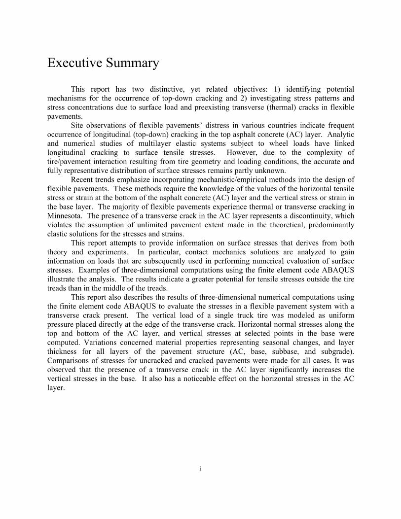
This report has two distinctive, yet related objectives: 1) identifying potential mechanisms for the occurrence of top-down cracking and 2) investigating stress patterns and stress concentrations due to surface load and preexisting transverse (thermal) cracks in flexible pavements. Site observations of flexible pavements’ distress in various countries indicate frequent occurrence of longitudinal (top-down) cracking in the top asphalt concrete (AC) layer. Analytic and numerical studies of multilayer elastic systems subject to wheel loads have linked longitudinal cracking to surface tensile stresses. However, due to the complexity of tire/pavement interaction resulting from tire geometry and loading conditions, the accurate and fully representative distribution of surface stresses remains partly unknown. Recent trends emphasize incorporating mechanistic/empirical methods into the design of flexible pavements. These methods require the knowledge of the values of the horizontal tensile stress or strain at the bottom of the asphalt concrete (AC) layer and the vertical stress or strain in the base layer. The majority of flexible pavements experience thermal or transverse cracking in Minnesota. The presence of a transverse crack in the AC layer represents a discontinuity, which violates the assumption of unlimited pavement extent made in the theoretical, predominantly elastic solutions for the stresses and strains. This report attempts to provide information on surface stresses that derives from both theory and experiments. In particular, contact mechanics solutions are analyzed to gain information on loads that are subsequently used in performing numerical evaluation of surface stresses. Examples of three-dimensional computations using the finite element code ABAQUS illustrate the analysis. The results indicate a greater potential for tensile stresses outside the tire treads than in the middle of the treads.
This report also describes the results of three-dimensional numerical computations using the finite element code ABAQUS to evaluate the stresses in a flexible pavement system with a transverse crack present. The vertical load of a single truck tire was modeled as uniform pressure placed directly at the edge of the transverse crack. Horizontal normal stresses along the top and bottom of the AC layer, and vertical stresses at selected points in the base were computed. Variations concerned material properties representing seasonal changes, and layer thickness for all layers of the pavement structure (AC, base, subbase, and subgrade). Comparisons of stresses for uncracked and cracked pavements were made for all cases. It was observed that the presence of a transverse crack in the AC layer significantly increases the vertical stresses in the base. It also has a noticeable effect on the horizontal stresses in the AC layer.
i
CHAPTER 1 - Introduction
Longitudinal surface cracks are predominantly parallel to the asphalt concrete pavement centerline and located in the vicinity of the wheel paths. Unlike fatigue cracking at the bottom of the asphalt concrete (AC) layer, inspections of core samples show that longitudinal cracks form from the surface and move downward. Forensic analyses also show that these cracks seldom reach the bottom of the AC layer
At the Minnesota road research facility, Mn/ROAD, longitudinal cracks have been observed to form perpendicular to the edge of the transverse cracks in the wheel paths, and then propagate away from the transverse cracks until they eventually meet and form one continuous crack the entire length of the pavement cell. At the early state of the distress, the cracks appear as hairline. The cracks are most visible in the spring and tend to heal over the course of the summer. Longitudinal cracking or, as it is sometimes called top-down cracking is now developing in all the Mn/ROAD mainline test cells and will likely continue to progress.
Longitudinal surface initiated cracking in flexible pavements has been observed not only in the United States, but worldwide. The conventional studies in pavement performance modeling are focused mostly on classical fatigue cracking initiated at the bottom of the AC layer. Several researchers have concluded that the conventional approach to analyzing pavement distress cannot explain surface-initiated top-down cracking, and have proposed various hypotheses in an attempt to explain this phenomenon. One of the most widely accepted hypotheses is that surface cracking is wheel-induced cracking. This implies that the problem should be addressed in terms of contact mechanics, since the tire properties and geometry affect the induced stresses. Most importantly, there is a significant effect from the tire treads.
The available analytical tools for pavement design and performance evaluation are based on the assumption of uniform pressure distributions exerted on the pavement surface by tires. Furthermore, the continuity of lateral strains in a multilayered pavement system is assumed. Recent research (2, 4, 6, 16, 20, 21, 22, 25, 27, 29, 30, 34) on the nature of near-surface stress distribution has shown that significant tangential (frictional) forces can be imparted to the pavement surface by truck tires. Estimates of the magnitude of these forces suggest that they may be sufficient to cause large tensile/shear stresses and localized failure near the pavement surface resulting in top-down propagating cracking.
With the increasing interest in the mechanistic/empirical design of flexible pavements, such as MnPave (1), information is needed to assess the distribution and magnitude of stresses and strains in the system’s various layers. In particular, tensile stresses (or strains) in the AC layer, and compressive stresses (or strains) in the base or subgrade, often are viewed as critical input values. The basis for determining the stresses and strains is the linear theory of elasticity, with analytic formulae, graphs, or computer software available to aid in calculations. The fundamental assumption in computing the stresses and strains, besides neglecting the unit weight, is the unlimited and continuous lateral extent of the pavement system. With this assumption, warranted by the relatively small contact area between tire and pavement surface in relation to pavement width, it is possible to make use of multilayer elastic half-space solutions. The assumption fails, however, if the AC layer is discontinuous, as is the case in the presence of
1

transverse cracks. Transverse cracks form due to asphalt shrinkage when the temperature decreases and usually extend across the whole width and depth of the AC layer. Theoretical analyzes of continuous flexible pavement systems have been presented by several researchers (2, 3, 4, 5, 6). Generic computer codes such as ABAQUS (7, 8), or specialized computational modules such as CIRCLY (9), BISAR (10), and ILLIPAVE (11), provide valuable tools for stress, strain, or displacement calculations. In contrast to the analysis of discontinuous rigid pavements with cracks or joints, limited references describe the effect of cracks on the behavior of flexible pavements; notable results on deflection profiles are reported by Uddin et al. (12) and Uddin and Pan (13).
The objective of this research was to investigate the interaction of truck tires and flexible pavement structures by means of analytic and numerical methods. More specifically, it investigates the stress patterns and stress concentrations due to surface load and identifies the important factors affecting surface stresses in pavement as possible causes of surface-initiated cracking. Another objective was to investigate the effect of transverse cracks on stresses at selected cross sections and locations in flexible pavement systems.
Empirical data from literature will be assessed critically to extract the main features of surface-initiated and transverse cracking distress. Next, analytic elastic models will be used to determine the differences in modeling the tire/pavement contact problem as a plain strain, axisymmetric, or three-dimensional problem. The results will form a reference for numerical models to be developed.
A numerical elastic multilayer model will be developed that allows for determining the stresses at the surface of the pavement as well as within the pavement. ABAQUS, a finite element computer code, will be used as a calculation tool. The factors influencing the stress distributions and the occurrence of tensile stresses will be investigated.
Appendix A presents the simulation matrix (55 cases) used for this research when a transverse crack was present. Appendix B discusses in detail the procedure required for completing (i.e. creating a model in ABAQUS/CAE to processing the output) one case study. Appendix C contains the summary cross sections for all 55 cases when a transverse crack is present.
The sign convention used for the results’ presentation is that compression is denoted by positive values and tension by negative values. This sign convention is compatible with the sign convention used in the mechanistic model of MnPave (1).
2
CHAPTER 2 - Literature Review
2.1 Introduction
The literature review for this research is divided into three sections: 1) field observations of longitudinal cracks, 2) experimental results for tire/pavement interfacial stresses, and 3) tire/pavement interaction models. The first section contains observations from experimental work performed in the area of longitudinal cracks. The second section presents experimental work done to determine tire/pavement interfacial stresses. Finally, the third section addresses analytic and numerical models used to describe tire/pavement interaction and the determination of stresses or strains in the pavement.
2.2 Field observations of longitudinal cracks
Gerritsen et al. (13) conducted a field study in the Netherlands on the occurrence of surface cracking in asphalt pavements, and on the potential causes of surface cracking. Static indirect tensile tests were performed on core samples collected; they showed that the asphalt concrete outside of the wheel paths tended to have low strength characteristics at low temperatures.
Dauzats and Rampal (14) surveyed several pavement sections located in the south of France. In this area, pavements are subjected to extreme thermal stresses. Longitudinal surface cracks in these sections were observed 3 to 5 years after construction of the road containing a slow lane and a fast lane. The longitudinal cracks were located on the centerline side of the slow lane. Dauzats and Rampal (14) also observed that the appearance of cracks fluctuated with the seasons.
Matsuno and Nishizawa (15) examined longitudinal surface cracking in asphalt pavements in Japan. Their study hypothesized that longitudinal surface cracks are induced by transverse tensile strains in the pavement close to the tire edges at high temperatures. Visual observations indicated that the cracking appeared 1 to 5 years after the road’s construction. The cracks typically occurred in the passing lane. It was also observed that the cracks were within or very close to the wheel paths. In addition, cracks did not appear in shadowed areas such as near an overpass bridge. Matsuno and Nishizawa (15) concluded from the visual survey that cracks had a higher rate of occurrence in higher temperatures.
Myers et al. (6) examined eight pavement sections in Florida having different levels of surface-initiated longitudinal cracking. The pavements ranged from 5 to 10 years in age. The thickness of the asphalt concrete layer ranged from 50 mm to 200 mm (2 in. – 7.9 in.). Longitudinal cracking was visible on one or both sides of both wheel paths. Crack widths at the surface were approximately 3 mm to 4 mm (0.12 in. – 0.16 in. ), and the cracks appeared to close with depth. The opening of the cracks also suggested that the primary mode was tensile cracking. Crack depths varied from about 25 mm (0.98 in.) to the whole thickness of the asphalt concrete layer. Cracking was observed in sections with no surface rutting and in sections where some rutting was present. 3

Bensalem et al. (16) performed field observations to study surface cracking in flexible pavements in the United Kingdom. A study of numerous cores revealed that surface cracks were present in pavements at least 160 mm (6.3 in.) thick. Overall, it concluded that bottom-up cracking was rarely the main failure mechanism. Instead, surface cracking was the main failure mechanism.
Uhlmeyer et al. (17) examined top-down cracking in asphalt concrete wearing courses in the eastern part of Washington State. It was observed that the cracks stopped at the interface between the wearing course and underlying bituminous layers. The authors found the typical crack geometry to be 3-4 mm (0.12 in. to 0.16 in.) wide and 47 mm (1.85 in.) deep. The width of the cracks decreased as depth increased, implying a v-shaped crack. They concluded that surface-initiated cracking located within or near the wheel paths occurs in pavement layers exceeding 160 mm (6.3 in.) thick. In the sections of pavement studied, the cracks appeared in the surface 3 to 8 years after construction.
Mn/DOT (18) performed visual surveys of longitudinal surface initiated cracking at their Mn/ROAD research facility. The results indicate that the surface cracks continue to increase as the years pass. Cracking was observed in both the driving lane and the passing lane; however, no conclusion can be derived about which pavement element (i.e. asphalt layer thickness, base) is more or less conducive to longitudinal surface cracking.
Zhang et al. (19) compared crack growth rates observed in the field to those measured in indirect tension tests. This study inspected longitudinal surface-initiated cracks in wheel paths in north central Florida. Seven of the 8 sections had surfaces 10 to 14 years old, while the eighth section had a surface age of 5 years. The asphalt layers ranged in thickness from 120 mm to 220 mm (4.7 in. to 8.7 in.). The results of the crack growth rate comparison between laboratory cracks and field cracks showed no close correlation.
2.3 Experimental results for tire/pavement interfacial stresses
Markwick and Starks (20) measured the contact stresses between light-weight truck tires and pavement. The inflation pressure was 0.28 - 0.35 MPa (40 to 50 psi). The authors concluded that the local contact normal stresses induced by a pneumatic tire were approximately 1.5 times higher than the inflation pressure. The normal stresses appear to be independent of truck speed. Shear stresses were directed inwards. Under a solid tire, the shear stresses were directed outwards.
Seitz and Hussmann (21) performed experimental studies on a radial-ply passenger car tire without profile. The authors observed inward shear stresses along the contact. The authors concluded that these stresses are due to sidewall bending (pneumatic effect), and that the compression of tread rubber (Poisson's effect) only reduces the magnitude of contact shear stresses due to bending but not their direction.
Lippmann (22) measured the distribution of stresses between the tread of the passenger radial-ply tire and pavement. The author noticed that bulging of the tire results in inward shear stresses at the edge of the tire.
Sebaaly and Tabatabaee (23) tested radial-ply, bias-ply and wide-base radial-ply single tires using different levels of inflation pressures from 0.52 to 0.76 MPa (75 to 110 psi). Only one value of contact pressure was recorded for each tread. The authors reported that the contact pressure distributions were nonuniform, with maximum contact pressures of 1.75 times the
4

inflation pressures. The maximum contact pressures were obtained along the center tread for all three tires, and the minimum contact pressures were obtained along the outer tread.
Huhtala et al. (24) measured contact pressure for two twin tires, and three twin tires. Tire pressure was varied from 0.48 to 1.08 MPa (70 to 157 psi). For passenger car tires, the contact pressures reached maximum at the edge. On the other hand, for truck tires, the contact pressures attained a maximum at the tire’s center.
Pottinger (25) measured contact stresses for both solid and passenger radial-ply tires with no profile in rolling and stationary modes. The author concluded that there were fundamental differences between these two tires. For the pneumatic tire, there was high normal stress at the tire’s edges, whereas, for the solid tire, the normal stresses were approximately uniform through the entire contact area. Shear stresses induced by the pneumatic tire were directed towards the center of the tire, with the maximum at the edge. Shear stresses induced by the solid tire were directed towards the edge of tire, again with the maximum at the edge.
Tielking and Abraham (26) tested three types of heavy radial-ply truck tires: a smooth tire, a conventional truck tire, and a wide-base truck tire. Inflation pressure varied from 0.55 to 0.90 MPa (80 to 131 psi). The authors noticed that the average contact pressure on each tread was higher than inflation pressure. No shear stresses were reported. In all cases, maximum contact pressures were located at the tire’s center.
DeBeer et al. (27) conducted tests on pavement structures having surfacing layers less than 50 mm (2 in.). The authors noticed that the shear stresses induced by the tires were directed towards the tire’s center, with zero value at the center. An increase in load resulted in an increase in the contact stresses at the tire edges, while an increase in inflation pressure resulted in an increase in the contact stresses at the center of the tire.
Myers et al. (28) measured tire contact stresses for bias-ply, radial-ply, and wide-base radial-ply tires. The inflation pressure varied from 0.62 to 0.96 MPa (90 to 140 psi). For the bias-ply tire the maximum vertical normal stress occurs at tire edges, whereas, for the radial-ply tire, the maximum normal stress occurs at the center of the tire contact area. The bulging of the sidewall of bias-ply tires induced inward contact shear stresses, whereas the radial-ply sidewall displayed minimal bulging effect. The authors asserted that because of Poisson's effect, tire treads tend to pull apart the surface of the pavement, which causes surface cracking.
Pottinger and McIntyre (29) performed experimental studies on passenger car and heavy-duty radial-ply truck tires. The tires were inflated to 0.26 MPa (38 psi) and 0.86 MPa (125 psi), respectively. The authors concluded that all tire treads induced outward shear tractions on the contact surface due to Poisson's effect. However, passenger car tire induced additional inward shear tractions due to pneumatic effect. For the heavy truck tire, no significant inward shear tractions due to pneumatic effect were observed.
2.4 Tire/pavement interaction models Gerritsen et al. (3) performed linear-elastic multi-layer analysis using the CIRCLY computer program. A vertical uniform contact pressure of 0.7 MPa (102 psi) and radial inward shear stresses of 0.35 MPa (51 psi) were considered to represent the stresses of the dual tire contact with a pavement structure. The asphalt concrete layer thickness ranged from 155 mm to 170 mm (6.1 in. to 6.7 in.). The base layer thickness ranged from 80 mm to 500 mm (3.1 in. to 19.7 in.), and the sub-grade layer thickness varied from zero to 1000 mm (39.4 in.). The authors found from the analysis that radial inward contact shear (tractions) stresses were capable of 5

initiating surface cracks. The authors concluded that traffic loads initiate the cracks and the environmental conditions propagate the crack.
Matsuno and Nishizawa (15) performed axisymmetric elastic finite element analysis with uniform normal contact stress representing the entire tire contact pressure. The radius of the load was 150 mm (5.9 in.) and two pavement structures were considered in the analysis. The first had an asphalt thickness of 200 mm (7.9 in.) and a cement-stabilized base thickness of 250 mm (9.8 in.). In the second, the asphalt thickness was 100 mm (3.9 in.) and the base thickness was 350 mm (13.8 in.). The modulus of asphalt concrete varied from 100 MPa (14504 psi) to 2000 MPa (290,076 psi). The modulus of base layer varies from 700 MPa (101,526 psi) to 2000 MPa (290,076 psi). The Poisson's ratio of 0.35 was kept constant. From the analysis, the authors concluded that the strains under the tire are mainly compressive in the vertical direction, and high lateral tensile strains at the tire edge were sufficient to cause cracking.
Perdomo and Nokes (30) used the computer program CIRCLY to examine the response of a flexible pavement system due to different loading. Two types of loading were considered: nonuniform normal tractions only and nonuniform normal tractions accompanied by nonuniform inward shear tractions. In both cases the load was applied to a contact area representing the entire tire contact area. The authors concluded that when inward shear tractions were considered in the analysis, the maximum tensile strains occur on the surface of the pavement at the edges of the tires.
Jacobs (31) analyzed the stresses in a pavement structure consisting of three layers, with constant thickness for each layer, one Poisson's ratio for all layers, the same elastic modulus for base and subgrade layers, and three different elastic moduli for the AC layer. In the analysis the computer program BISAR was used. The stresses applied, both normal and tangential, were obtained from experiments on a bias-ply truck tire. The experimentally measured stress distributions were subdivided into a finite number of circular cells, each carrying uniform stresses. The author concluded that the normal stresses at the bottom of the asphalt concrete layer were not affected by the tangential stress on the surface. The tensile stresses at the edge of the loaded area can be much higher than the tensile stresses at the bottom of the asphalt concrete layer. These tensile stresses can cause longitudinal surface cracking.
Collop and Cebon (2) examined the potential of longitudinal surface fatigue cracking in asphalt pavements using different analytic and numerical solutions. From 2D plane strain elastic half-space solution, the author concluded that there is singularity in surface stresses at both ends of the contact if a discontinuity in shear tractions is assumed. A triangular shear tractions distribution does not produce singularities at the loaded edge. In the FE model, uniform normal contact pressure acting over a circular contact area, and an inward shear contact traction varying linearly from zero at the center of the tire towards a maximum value at the tire edge were considered. From the analysis, the authors concluded that shear tractions between the tire and the pavement induce high local tension around the edge of the contact patch, which may lead to surface longitudinal cracks that propagate by thermal fatigue.
DeBeer et al. (27) studied the effects of nonuniform contact stresses on thin asphalt surfacing layer of 40 mm (1.6 in.) thick. An axisymmetric finite element solution was constructed. The diameter of the loaded area was 200 mm (7.9 in.). Several types of loading conditions were considered: nonuniform normal stress, inward shear stress, and outward shear stress. The authors applied discontinuous shear stresses at the edge of tread. The authors concluded that tensile stresses developed outside the tire contact area.
6
Myers et al. (6) performed studies on the potential mechanisms of surface cracking. The stresses in the pavement were determined using the program BISAR. Asphalt concrete thickness and modulus were varied in their study; base thickness remained constant, but modulus varied, and the subgrade had constant modulus. The interface between each layer was modeled both in full slip and full contact. Tire/pavement contact stress distributions were obtained from experimental data on radial-ply truck tire provided by Pottinger (24). Each tire tread was modeled with at least 2 circles across. The direction of uniform shear tractions was taken as pointing outward due to Poisson's effect of each tread. The authors concluded that the location where the maximum surface tensile stresses occur is the center of the outer treads, rather than the edge of the tread. The magnitude of the predicted tension appears to increase with the width of the tire tread, with the highest tension found under the center of the widest tread.
Roque et al. (32) investigated the adequacy of tire contact stress measurements using instrumented steel bed (28) for evaluation of loads exerted on typical highway pavement structures. A two-dimensional FE model was used to model a typical radial tire and a pavement structure. The tire and steel bed were assumed to be fully bonded, and the tire tread was taken as 203 mm (8 in.) wide and 36 mm (1.4 in.) high. The asphalt concrete surface layer thickness was 100 mm (3.9 in.) with the Easphalt/Ebase ratio of 4 to 40. Uniform pressure was applied to the top of the tread. It was concluded from these studies that the contact stresses measured using devices with rigid foundations are suitable for the prediction of response and performance of highway pavements.
Bensalem et al. (16) considered a three-dimensional multi-layer elastic finite element model with fully bonded layers. The top layer (asphalt surface course, the binder course, and the road base) had a range of thickness from 200 mm (7.9 in.) to 400 mm (15.7 in.). The sub-base was 300 mm (11.8 in.) thick. The authors found that in thin pavements it appears that the tire induced contact shear stresses were unlikely to cause surface cracks in the close vicinity of the wheel path. Thicker pavements, on the other hand, were more susceptible to surface cracking from wheel loading as the tensile surface stresses were significant.
Svasdisant et al. (33) considered three different modeling methods. The first was a 2D closed-form solution computer program, CHEVRONX. The second was a 2D finite-element computer program, MICHPAVE. The third was a 3D ABAQUS model. In all cases, uniform normal loading was applied. The authors found that the magnitude of the surface tensile stresses increases as the thickness of asphalt concrete layer decreases.
Perret (34) performed 3D finite-element modeling of a layered pavement system. The reference load used was a super-single tire with 0.8 MPa (116 psi) of inflation pressure. Special elements were used to model infinite boundary conditions and interface properties. The loaded area was a 135 x 135 mm (5.3 in. x 5.3 in.) square. Various loading conditions were considered: uniform normal, uniform normal at the center with a sudden increase at the edges of the loaded area, and inward shear linearly decreasing towards the center and others. The author found that the distribution of the normal load influences the location of the maximum horizontal surface stress, but not the horizontal strains. With shear tractions applied, the stresses around the loaded edge are tensile, but insufficient to cause cracking. The author concluded that it seems impossible that a shear contact stresses load could induce enough horizontal tensile stresses to overcome the compressive stresses induced by the normal contact stresses to initiate top-down cracking.
Uddin and Pan (13) studied the correlation between computed dynamic deflections in a flexible pavement using the finite-element code ABAQUS to measured dynamic deflections in a 7

flexible pavement from the falling weight deflectometer (FWD) test. To do this, the authors used a three-dimensional multilayer pavement model in ABAQUS that was developed by Uddin et al. (12) during previous related work. The model was 26.62 m long, 9.15 m (360.2 in.) wide, and 12.80 m (504 in.) high. The model consisted of 11,877 three-dimensional brick elements. The mesh was not uniform, but composed of a fine mesh around the loaded area (since this was the region of interest) and a coarse mesh away from it. The boundary conditions for the model consisted of a fixed bottom and rollers along the sides to prevent horizontal displacement. The load applied to the model was representative of a FWD pulse, with a force of 40 kN (9000 lbf) distributed over an area of 0.0706 m2 (109.4 in.2). Uddin and Pan (13) found that there was a good match between the calculated ABAQUS dynamic deflections and the measured FWD deflections. The authors then introduced a crack, either a longitudinal, transverse, or alligator crack, into the model using the special-purpose gap elements available in ABAQUS. The crack was modeled with a gap of 0.25 mm (0.01 in.) and a friction coefficient of 0.5 between the two contact surfaces. This was the maximum gap that still produced interaction between the two surfaces when loaded. The maximum dynamic deflections were calculated for each of the differently cracked pavements and compared to the calculated deflection of an uncracked pavement. When a longitudinal crack was present, the pavement experienced a deflection increase of approximately 17% compared to the calculated deflection of an uncracked pavement. The pavement displayed only an increase in deflection of 10% when a transverse crack was present. When a pavement had severe alligator cracking, the calculated deflection was about 36% higher than the calculated deflection for an uncracked pavement.
In the paper by Cho et al. (35), the authors compared three types of finite-element models: plane strain, axisymmetric, and three-dimensional. The commercial program ABAQUS was used to derive the FEM solution. The layered elastic-theory program BISAR was used for comparison results. A comparison was made between the maximum vertical deflection and the horizontal tensile stress in the bottom of the pavement layer to determine the accuracy of the FEM model. The plane-strain model used a relatively fine mesh for analysis, because the pavement surface was quite thin in comparison to the thickness of the subgrade. The total depth of the model was 2.3 m (90 in.). The load applied to the model was equal to a 40 kN (9000 lb) point load applied at the center node of the model (!). The boundary conditions of the model were that each side was fixed from horizontal displacement and the bottom was completely fixed. The authors used three different configurations of axisymmetric models. The first two models had the same dimensions of 2.3 m by 2.3 m (90 in. by 90 in.). The boundary conditions were also the same, having zero horizontal displacement on the side of the model and the bottom was encastre (fixed). The only difference was that one model had four times more elements than the other. The third axisymmetric model incorporated the use of infinite elements at the boundaries of the pavement structure instead of imposing boundary conditions on them. The load for all three models was 567.4 kPa (82.3 psi) acting over a circular area with a radius of 0.15 m (6 in.). The axisymmetric model with infinite elements at the boundaries produced better solutions compared to the solutions from the models with imposed boundary conditions. When a transverse crack or longitudinal crack is present the axisymmetric model cannot be used to represent the pavement system. A three-dimensional FEM model was also investigated by the authors. Cho et al. (35) modeled the loaded area as a rectangular shape. The boundary conditions for the sides of the model were roller supports, so there was no horizontal displacement. The bottom of the model was completely fixed. A maximum of 16,200 elements for linear 3-D solid elements and 2,000 elements for quadratic elements were used due to 8

computer-memory limitations. The three-dimensional FEM model produced results that matched well to the layered elastic-theory solution. Tabatabaie and Barenberg (11) developed a finite-element computer program, ILLI-SLAB, to determine stresses and deflections in jointed or cracked concrete pavements. This program is based on the classical theory of a medium-thick plate on a Winkler foundation. It allows for analysis of slabs with different thicknesses. The program can also evaluate slabs with different joint designs, such as free edge, doweled, aggregate interlock, thickened edge, or tied key joints. The finite element solutions were compared to theoretical solutions (e.g., Westergaard’s solution), as well as experimental studies (e.g., AASHTO road test) to assess the accuracy of ILLI-SLAB. The results from the ILLI-SLAB model showed good correlation with Westergaard’s equations for an infinite slab (36). For multiple loading of a slab, influence charts developed by Pickett and Ray (37) were used by the authors to compare to the FEM results. Once again, good correlation was observed between the results from the FEM and the influence charts. Zaghloul and White (38) used a three-dimensional, dynamic finite-element model created in ABAQUS, to evaluate the response of flexible pavements to moving loads at various speeds. Different material models were used to represent diverse pavement structures. The authors used the Drucker-Prager model to model granular and silty materials and the Cam-Clay model for clayey soils. The asphalt concrete was modeled as a viscoelastic material. The mesh was non-uniform and consisted of 5,278 elements. The boundary conditions for the sides of the model parallel to the direction of traffic were zero displacements. For the sides perpendicular to the direction of traffic, free boundary conditions were introduced, because the model was sufficiently long that those edges did not affect the pavement response. The bottom of the model had fixed boundary conditions. To verify that the 3D-FEM model was acceptable for pavement analysis, both static analysis and dynamic analyses were used. First, Zaghloul and White (38) compared the results from the static analysis of the 3D-FEM model with the results of a multilayer elastic analysis using BISAR. They found that there was high linear correlation between the results from the 3D-FEM model and those from the multilayer elastic analysis. To further validate the 3D-FEM model and its nonlinear analysis capabilities, a dynamic analysis was conducted, and the results were compared to actual measurements of pavement deflections. The authors concluded that there was no difference between the computed deflections and the measured deflections. Zaghloul and White (38) also conducted a sensitivity analysis to study the effect of cross section and load parameters on pavement response. They found that the confinement of the shoulders and the continuity of the pavement-shoulder joint reduced deflection, and that other parameters such as temperature, loading time, and rate of loading also had an effect on the pavement response.
9

10

CHAPTER 3 – Tire Pavement Interfacial Stresses
3.1 Modeling tire/pavement interaction
In general, one can use two approaches to model the interaction between the stationary or moving tire and a pavement structure. The first, and more rigorous approach, the contact mechanics approach (39), considers two elastic bodies in contact; When two elastic bodies are in contact, the actual contact area and the distribution of tractions (normal, σn, and tangential, τn) at the interface are unknown before solving the problem and are part of the solution. The tractions, and the stresses and strains in the bodies, depend on the elastic and geometric properties of both solids and external load. Furthermore, if the contact surface changes with load, the principle of superposition often used in elasticity is not applicable.
For simple geometries contact problems, analytic solutions for plane strain, axisymmetric, and some three-dimensional cases are found in literatures (40, 41, 42, 43, 44, 45, 46). Several numerical techniques, such as finite-element and finite-differences, are used to solve in more general cases. However, when using numerical techniques, special elements or a very fine mesh are required to allow good resolution that is necessary for capturing the occurrence of high gradients in stresses or strains, and the possibility of singularities that analytic solutions account for directly.
On the other hand, one can approximate the two-solid contact problem by a single-solid problem with specified surface tractions or displacements (2, 4, 5, 6, 16, 28, 32, 35, 47, 48, 49). In other words, one of the solids in contact, in this case the tire, is replaced by an assumed distribution of tractions or displacements. Obtaining solutions for the single-solid problem, either analytically or numerically, is relatively simple; the superposition principle applies, and many fundamental solutions can be found in the literature. However, the outcome of this approach strongly depends on the assumed distribution of surface tractions or displacements. Therefore, the outcome is only meaningful when the actual distribution of tractions or displacements is known reasonably well.
3.2 Fundamental concepts of contact mechanics The geometry (profile) of two elastic bodies coming into normal contact plays a major role in the stress and strain distributions within the bodies (39). For example, if the profile of both bodies changes smoothly through the boundary of contact, the normal interfacial tractions σn approach zero at the edges of contact, Fig. 3.1a. This fundamental principle is derived from a geometric condition, which states that the continuously smooth surfaces should not interfere outside the growing contact area when the compressive load increases. This principle is also valid if one of the profiles displays high curvature. In this case, the tractions σn have a high gradient from the zero-value at the edge of contact, Fig. 3.1b.
In the case where interfacial friction is present, the geometric compatibility condition still holds, and the shear tractions τn are zero at the contact edges. The rate of τn approach to zero-value at the edge depends on the local curvature outside the contact. For symmetrical external
11
loading, the distribution of tractions τn is mathematically antisymmetric, with zero-value at the center. The direction of τn depends on the ratio R of the contact area dimension, Lc, to the lateral dimension of the smaller solid, Ls, and on the compliance of the solids. If R = Lc/Ls << 1, τn points inward on the surface of the stiffer solid, and outward on the softer one; Fig. 3.1a shows the tractions acting on the stiffer solid. Conversely, if R = Lc/Ls ≈ 1, tractions τn point outward on the surface of the stiffer solid and inward on the softer one, Fig. 3.1b. The latter may apply to tire-pavement interaction, where the tire is the softer solid and the asphalt concrete is the stiffer solid. It is important to note that the ratio of τn to σn rises to infinity at the edge of the contact area, which implies that some slip next to the edge should occur. This phenomenon, in the case of repeated loading, is referred to as fretting fatigue. Also note that these properties are preserved even if external loading is inclined.
On the other hand, if the profile of one of the surfaces changes abruptly at the edge of contact (sharp corner), the tractions σn become infinitely large, and it is said that the solution is singular, Fig. 3.1c. The order of singularity (rate of approach) depends on the elastic parameters of the bodies, and the corner angle. This also applies to tractions τn in the presence of friction, and to inclined loading.
12

FIGURE 3.1 Surface tractions acting on a stiff solid in contact problems: (a) continuous profile R = Lc/Ls 1; (b) continuous profile R = L= c/Ls ≈ 1 and (c) discontinuous profile R = Lc/Ls ≈ 1
13

14

CHAPTER 4 – Analytical Solutions
In this section, the differences in two-dimensional (plane strain) and three-dimensional (axisymmetric and non-axisymmetric) analytic modeling of lateral stresses induced by normal and shear tractions acting on the surface of uncracked flexible pavements are discussed. The understanding of these differences is crucial in selecting an appropriate finite-element method (FEM) scheme that will help in analyzing the potential for top-down cracking. Also, the analysis provides benchmarks for verifying FEM solutions. Several loading configurations are studied and the results of surface horizontal stresses are compared. All configurations pertain to homogeneous elastic half space for which analytic solutions exist. These were taken from the literature (39, 49, 50, 51), where, besides mathematical formulae, useful tables of coefficients are provided.
4.1 Vertical strip load
The problem of a line of concentrated force applied perpendicular to the surface of an isotropic elastic half-plane is known as Flamant's problem, Fig. 4.1. The horizontal normal stress can be determined from the following expression
2
2 2
2( )
zxx
F x z2x z
σπ
=+
(0.0.1)
where Fz represents a line of force applied along the y-axis and has dimensions of force/length. Notice that Eq. (4.1.1) does not contain any elastic parameter. For a constant distribution of traction p, the Flamant's solution when integrated over a width 2b gives
[ sin cos( 2 )xxp ]σ α α α δπ
= − + (4.1.2)
The angles α and δ are defined in Fig. 4.2. Again, the horizontal normal stress is independent of elastic parameters, zero on the surface outside the loaded area, and constant inside the loaded area. It can be shown that, by approaching this point from different radii, the horizontal normal stresses attain different values, Fig. 4.3. The horizontal normal stress distribution is shown in Fig. 4.4.
15

FIGURE 4.1 Flamant’s problem
FIGURE 4.2 Uniform vertical strip load
16

FIGURE 4.3 Stresses at singular point
FIGURE 4.4 Horizontal normal stresses due to uniform vertical strip load
17

4.2 Horizontal strip load
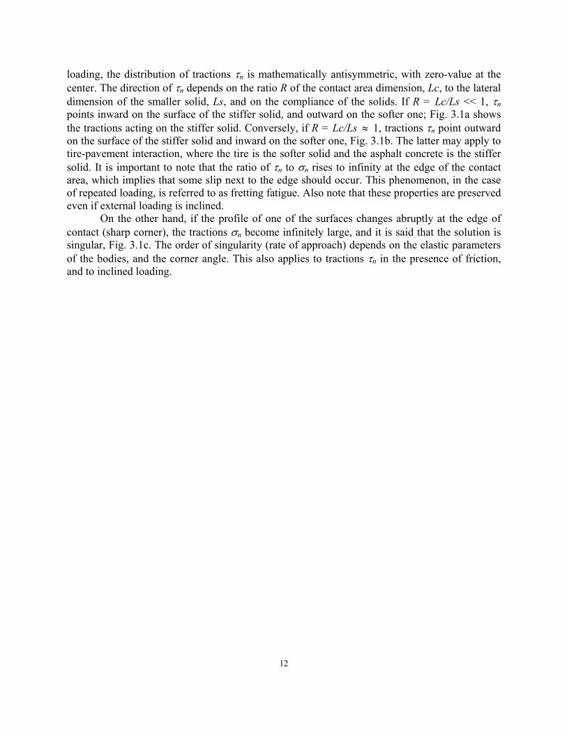
The horizontal normal stresses in half-plane due to uniform distribution of horizontal tractions over a strip can be found in the same way as for uniform vertical tractions (39). The horizontal normal stresses due to uniform horizontal tractions are given as
2
122
ln sin sin( 2 )xxRqR
σ α α δπ
= − +
(0.1.1)
where 2
1R , 22R , α , and δ are depicted in Fig. 4.5. The discontinuity in q at the edge has a
different effect than discontinuity in p at the edge. The logarithmic term in Eq. (0.1.2) leads to an infinite value of σxx, tensile at O1, and compressive at O2. The horizontal normal stress distribution is shown in Fig. 4.6.
FIGURE 4.5 Uniform horizontal strip load
18
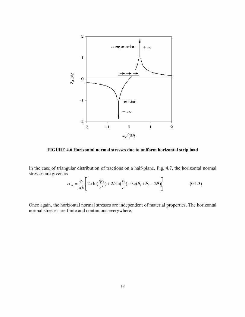
FIGURE 4.6 Horizontal normal stresses due to uniform horizontal strip load
In the case of triangular distribution of tractions on a half-plane, Fig. 4.7, the horizontal normal stresses are given as
0 1 2 21 22
1
2 ln( ) 2 ln( ) 3 ( 2 )xxq r r rx b zb r r
σ θ θ θπ
= + − +
− (0.1.3)
Once again, the horizontal normal stresses are independent of material properties. The horizontal normal stresses are finite and continuous everywhere.
19
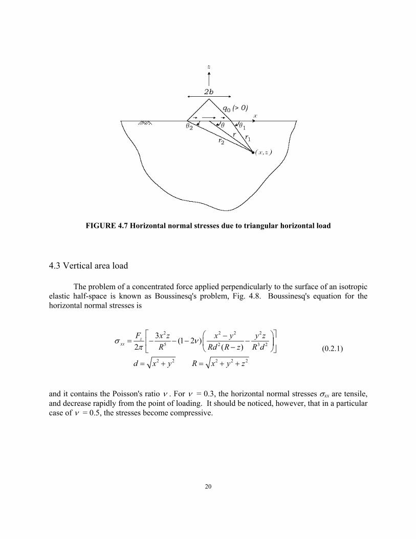
FIGURE 4.7 Horizontal normal stresses due to triangular horizontal load
4.3 Vertical area load
The problem of a concentrated force applied perpendicularly to the surface of an isotropic elastic half-space is known as Boussinesq's problem, Fig. 4.8. Boussinesq's equation for the horizontal normal stresses is
2 2 2
5 2
2 2 2 2 2
3 (1 2 )2 (
zxx
F 2
3 2)x z x y yR Rd R z R
d x y R x y z
σ νπ
−= − − − − −
= + = + +
zd (0.2.1)
and it contains the Poisson's ratio ν . For ν = 0.3, the horizontal normal stresses σxx are tensile, and decrease rapidly from the point of loading. It should be noticed, however, that in a particular case of ν = 0.5, the stresses become compressive.
20

FIGURE 4.8 Boussinesq’s problem
To determine the horizontal normal stress beneath and outside a circularly loaded area, the Boussinesq's equation is integrated, Fig. 4.9. The resulting formula is lengthy and is not presented here. It can be represented in the following form:
[ ]0 2 (1 2xx )p A C Fσ ν ν= + + − (0.2.2)
where the coefficients A, C, F are provided by Poulos and Davis (49). An alternative is to use one of the available softwares such as Weslea (52) or CIRCLY (9), which allow for calculating the horizontal normal stresses automatically. The results of a sample calculation for ν = 0.3 are shown in Fig. 4.10. It is seen that inside the loaded area the horizontal normal stresses σxx are compressive, and become tensile outside the loaded area. The tensile stresses at the edge have a maximum value of (1-2ν) p0 /3 and the compressive stresses at the center have the value of (1+2ν) p0 /2. The horizontal normal surface stresses σxx becomes indeterminate on the edge; however, this indeterminacy vanishes if p0 = 0 on the edge (50).
In the case of rectangular distribution of tractions on a half-space, the horizontal normal stresses are given by Love (50). Love shows that the component of shear stress τxy has a theoretically infinite value at the corner of the rectangle but elsewhere all the stress components are finite.
21

FIGURE 4.9 Uniform vertical circular load
s
b
FIGURE 4.10 Horizontal normal stresses due to uniform vertical load on circular region
22

4.4 Circular horizontal load
Stresses, strains, and displacements that are due to tangential tractions q0, on a circular region, can be found by integral transform methods (53, 54). The solutions are then evaluated using computer code CIRCLY (9). For uni-directional tangential tractions on a circular region, horizontal normal stresses are singular along the boundary of the loaded region. The horizontal normal surface stresses are infinite compression at O1 and infinite tension at O2, Fig. 4.11. The horizontal normal surface stress distribution is shown in Fig. 4.12.
FIGURE 4.11 Uniform horizontal circular load
23

FIGURE 4.12 Horizontal normal stresses due to uniform tangential load on circular region
For axisymmetrical tangential tractions on a circular region having finite q0 at the boundary, whether it is radially inward or radially outward, at the boundary of loaded region horizontal normal stresses σxx are infinite. However, for both cases, if the tangential tractions are zero at the boundary of loaded region, then horizontal normal stresses are finite, compressive for q0 acting outward, and tensile for q0 acting inward.
4.5 Summary of observations
Particular distributions of tractions that erroneously approximate the contact mechanics solutions may produce infinite stresses within the pavement. For example, the normal stresses σxx parallel to the contact become infinite at the surface if the single-solid problem is solved with tractions τn, whether it is plane strain or in axisymmetric, having a finite value of a finite loaded area, or if the tractions τn undergo jump within the loaded area, e.g., at the center. This is independent of the magnitude of τn, and applies to an antisymmetric distribution or one-way acting τn, Figs. 4.13a and 4.13b. This does not apply, however, to tractionsσn, whose finite value approximating high gradient at the edge of the contact yields finite normal stresses σxx, Fig. 4.13c.
The analysis above clearly demonstrates that the distribution of the horizontal normal stresses σxx depends on whether the problem is solved as two-dimensional (plane strain) or three-dimensional (axisymmetric and non-axisymmetric). Three-dimensional solutions give tensile
24

stresses at some locations. Additional tensile stresses at or near the surface may be caused by the lateral expansion of tire treads, which in the presence of surface friction provide surface shear stresses. Three-dimensional solutions incorporate the Poisson's ratio of the material.
25

FIGURE 4.13 Horizontal surface stresses xxσ due to (a) antisymmetric tangential tractions; (b) uni-directional tangential tractions and (c) normal tractions
26

CHAPTER 5 – Numerical Model 5.1 Introduction
Two different models were created in ABAQUS. The motivation for creating two different models derived from two different project goals: (1) investigation of the initiation of longitudinal cracks, and (2) the effect of a transverse crack on the stresses in the AC layer and base layer. To assure adequate accuracy of the computations for the first goal of the project, a model consisting of 1,000,000 elements had to be considered. Because the second goal of the project required consideration of a large number of cases (110), use of the model consisting of 1,000,000 elements was time prohibitive. Accordingly, a second model, consisting of 65,000 elements, was constructed, and its accuracy was verified as sufficient. In the following sections, these two models are described separately.
5.2 Modeling the pavement structure – longitudinal cracking
5.2.1 Modeling tire/pavement interaction
When referring to contact mechanics solutions in § 3.3, it must be remembered that they pertain to interaction between two solid bodies, and may not apply directly to interaction between the tire and pavement. In particular, most tires are pneumatic (hollow) rather than solid. As discussed in § 2.3, invaluable data are provided by experiments where local forces exerted by real tires on instrumented surfaces are measured at selected points, and the corresponding tractions acting over small areas are evaluated (20, 21, 22, 23, 24, 25, 26, 27, 28, 29).
In general, the experiments show the existence of both normal and tangential tractions. Regardless of the type of tire (truck, car, bias-ply, or radial-ply), the normal tractions σn are compressive, with their higher value measured either beneath the inner (crown) or the outer (shoulder) treads, Fig. 5.1 is a schematic reproduction of results reported by Pottinger and McIntyre (29) for rolling radial tires; note that Fig. 5.1 shows tractions acting on the pavement, and preserves the relative width of treads and intensity of stresses. For the truck tire tested, the inner treads carry normal tractions significantly greater than the outer treads (Fig. 5.1a). In the case of a passenger-car performance tire, all treads transmit approximately the same normal tractions (Fig. 5.1b). Higher normal tractions at passenger car tire shoulders were measured by Lippmann (22), and Huhtala et al. (24). A strong influence by inflation pressure and truck tire load was reported by DeBeer et al. (27).
Significant difference in the magnitude and direction is observed in the distribution of tangential tractions τn acting on the pavement, Fig. 5.1c. The tractions τn along the centrally located treads act away from the tread's center, and their distribution is close to antisymmetric with the zero-value at or near the center of the tread. On the other hand, the outer treads transmit tractions τn acting towards the center of the tire contact patch. This was clearly observed in tests 27

on a performance tire (Fig. 5.1d), and less visible with a truck tire (Fig. 5.1c). The inward direction of tractions τn was also reported by Pottinger (25) for a smooth (treadless) tire, and is generally attributed to narrowing of the pneumatic tire due to reduction in cord tension. This inward direction of tractions τn was not observed in a solid tire (25).
When analyzing Fig.5.1, the difference in the distribution of local and average traction σn and τn,, with the latter indicated in Fig.5.1 by a superposed bar, becomes apparent. The local tractions σn have values beneath treads higher than the inflation pressure, and nearly equal the inflation pressure when averaged over the whole tire width. The local tractions τn show distinct antisymmetric outward action beneath central treads and one-directional inward action beneath treads away from the center. The distribution of average tractions τn strongly depends on the averaging process and type of tire. If averaged over the whole tire width, the distribution of average τn for a performance tire is inward, and antisymmetric, and, for a truck tire, τn is of nearly zero-value. If, for the truck tire, local averaging is applied, only the outer parts carry small inward tractions τn.
The observations above indicate that in evaluating the surface horizontal normal stresses σxx, it is important to consider the local distribution of tractions σn and τn as measured in tests. This was appreciated, for example, by Jacobs (31) and Myers et al. (6). However, it is also important to make use of the information derived from contact mechanics when the measurements are inaccurate or missing. On the other hand, if the objective is to determine the stresses and strains away from the surface, e.g., at the bottom of asphalt layer or in granular base, the averaged tractions σn and τn will provide sufficiently accurate results. The averaged tractions may violate distributions resulting from contact mechanics.
28
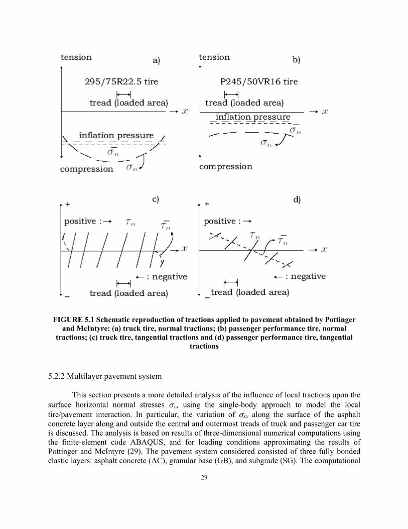
FIGURE 5.1 Schematic reproduction of tractions applied to pavement obtained by Pottinger and McIntyre: (a) truck tire, normal tractions; (b) passenger performance tire, normal
tractions; (c) truck tire, tangential tractions and (d) passenger performance tire, tangential tractions
5.2.2 Multilayer pavement system
This section presents a more detailed analysis of the influence of local tractions upon the surface horizontal normal stresses σxx using the single-body approach to model the local tire/pavement interaction. In particular, the variation of σxx along the surface of the asphalt concrete layer along and outside the central and outermost treads of truck and passenger car tire is discussed. The analysis is based on results of three-dimensional numerical computations using the finite-element code ABAQUS, and for loading conditions approximating the results of Pottinger and McIntyre (29). The pavement system considered consisted of three fully bonded elastic layers: asphalt concrete (AC), granular base (GB), and subgrade (SG). The computational
29

model, with dimensions 1.6 m (63 in.) in thickness, 1 m (40 in.) in length, and 1 m (40 in.) in width (symmetrical half of 1.6 x 1 x 2 m (63 in. x 40 in. x 80 in.) physical volume). The model was first subdivided into several elemental layers, partitions. These partitions allowed the thickness of the AC layer to be changed easily by specifying different material properties, instead of redrawing the model each time, Fig. 5.2. Over the vertical plane of symmetry, the nodal points were prohibited from moving out of plane. Over the remaining side and bottom of the prism, no displacements were allowed to take place in any direction (fixed supports), Fig. 5.2. Since the loaded area is much smaller than the entire model and the stresses of interest are near the vicinity of the loaded area, the effects of the above boundary conditions should be insignificant.
zero displacements
zero displacements zero normal
displacements (plane of symmetry)
FIGURE 5.2 Pavement structure
5.2.3 Finite-element mesh
The model was subdivided into one million (1,000,000) prismatic elements in the vicinity of the loaded area, Fig. 5.3, and tetrahedral elements close to the outer boundaries of the model. This made it possible to obtain the resolution of about 0.0004 m in depth next to the AC surface. The total thickness of AC and GB of 0.6 m (24 in.) was kept constant, while the thickness of AC layer varied from 0.05 m to 0.5 m (2 in. x 20 in.). A simplified, rectangular loaded area 0.02 x 0.2 m (0.8 in. x 8 in.) representing a single tread was selected, with 20 x 40 elements in plan.
30
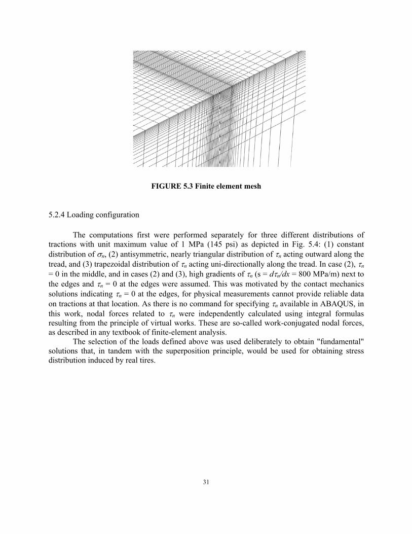
FIGURE 5.3 Finite element mesh
5.2.4 Loading configuration
The computations first were performed separately for three different distributions of tractions with unit maximum value of 1 MPa (145 psi) as depicted in Fig. 5.4: (1) constant distribution of σn, (2) antisymmetric, nearly triangular distribution of τn acting outward along the tread, and (3) trapezoidal distribution of τn acting uni-directionally along the tread. In case (2), τn = 0 in the middle, and in cases (2) and (3), high gradients of τn (s = dτn/dx = 800 MPa/m) next to the edges and τn = 0 at the edges were assumed. This was motivated by the contact mechanics solutions indicating τn = 0 at the edges, for physical measurements cannot provide reliable data on tractions at that location. As there is no command for specifying τn available in ABAQUS, in this work, nodal forces related to τn were independently calculated using integral formulas resulting from the principle of virtual works. These are so-called work-conjugated nodal forces, as described in any textbook of finite-element analysis.
The selection of the loads defined above was used deliberately to obtain "fundamental" solutions that, in tandem with the superposition principle, would be used for obtaining stress distribution induced by real tires.
31

FIGURE 5.4 Loading Configuration
5.2.5 Material parameters The following values of the elastic parameters selected by Mn/DOT, used in the MnPAVE Designer’s Guide, and corresponding to typical summer conditions in Minnesota, were used in computations: EAC = 1,766 MPa (256,100 psi), νAC = 0.38, EBG = 131 MPa (19,000 psi), νBG = 0.4, ESG = 43 MPa (6,200 psi), νSG = 0.45.
32

5.3 Modeling the pavement structure – transverse cracks The description of the numerical model of the pavement structure is divided up into three different sections. The first section describes the layered system of the pavement and its representation in the finite-element program ABAQUS. The second describes how the model is meshed (i.e., divided into discrete elements) efficiently. Finally, the third section discusses the material properties (i.e., Young’s modulus and Poisson’s ratio).
5.3.1 Layered system
The pavement system was modeled geometrically as a three-dimensional prism consisting of three or four layers: asphalt concrete (AC), base (B), subbase (SB, not included in all cases), and subgrade (SG). All layers are bonded, and each was modeled as an isotropic elastic material. The prism simulated a symmetrical half of the physical prism (road) cut by a plane perpendicular to a transverse crack. The bottom and three sides of the prism were immobilized (zero lateral and vertical displacements), and the remaining side representing the plane of symmetry was semi-fixed (zero lateral displacements). The outer dimensions of the prism, 1.0 m (40 in.) in width, 1.0 m (40 in.) in length, and 1.6 m (63 in.) in depth, were deemed sufficient to not affect the stresses and strains in the vicinity of the applied wheel load.
The eleven geometric structures provided by the Minnesota Department of Transportation (Mn/DOT) were representative of real pavement structures that were constructed at the Minnesota Road Research (Mn/Road) facility. In total, one hundred ten (110) cases of pavement systems, either without (55) or with a transverse crack (55) were considered. A complete listing of all cases (55) can be found in Appendix A. The asphalt concrete (AC) layer ranged from a thin layer of 0.1 m (4 in.) to a thick layer of 0.3 m (12 in.). The base layer varied from 0.076 m (3 in.) to 0.3 m (12 in.). If a subbase was included, it was 0.6 m (24 in.) thick. The subgrade varied from 0.55 m (21 in.) to 1.42 m (56 in.). Table 1 lists all of the layer thicknesses.
33

TABLE 1 Range of Layer Thicknesses
Asphalt concrete Base (Class 5)
Subbase (Select granular)
Subgrade (Clay loam)*
(Sand)**
0.1 m (4 in.) 0.076 m (3 in.) 0 1.42 m (56 in.)* 0.2 m (8 in.) 0.076 m (3 in.) 0 1.32 m (52 in.)*
0.3 m (12 in.) 0.076 m (3 in.) 0 1.22 m (48 in.)* 0.1 m (4 in.) 0.15 m (6 in.) 0.6 m (24 in.) 0.75 m (29 in.)* 0.2 m (8 in.) 0.15 m (6 in.) 0.6 m (24 in.) 0.65 m (25 in.)*
0.3 m (12 in.) 0.15 m (6 in.) 0.6 m (24 in.) 0.55 m (21 in.)* 0.1 m (4 in.) 0.076 m (3 in.) 0 1.42 m (56 in.)** 0.2 m (8 in.) 0.076 m (3 in.) 0 1.32 m (52 in.)**
0.3 m (12 in.) 0.076 m (3 in.) 0 1.22 m (48 in.)** 0.1 m (4 in.) 0.3 m (12 in.) 0 1.20 m (47 in.)* 0.2 m (8 in.) 0.3 m (12 in.) 0 1.10 m (43 in.)*
5.3.2 Mesh
Due to the large number of cases that had to be considered, an appropriate methodology for building the pavement structure model had to be selected and then employed using ABAQUS. To account for the varying layer thicknesses of all the layers, the pavement structure model was partitioned into 0.025 m (1 in.) and 0.05 m (2 in.) elemental layers. By partitioning the model into small increments, only one pavement structure model had to be created in ABAQUS, instead of eleven different models. The various physical thicknesses of each layer (i.e., AC, base/subbase, and subgrade) were obtained by assigning appropriate material properties to the elemental layers. Besides being partitioned into elemental layers, the pavement model had a partition that could represent a longitudinal crack if the material properties assigned were nearly zero. For this research, the option of introducing a transverse crack was needed. A partition in the pavement model representing a transverse crack was introduced. The crack was introduced by assigning nearly zero values for the material properties. In the pavement model shown in Figure 5.5, it appears that two transverse cracks were partitioned; only one was used as a transverse crack. The other was needed to insure that when the pavement was meshed, the mesh remained symmetric.
34

FIGURE 5.5 Partitioned pavement structure model in ABAQUS
Each elemental layer was subdivided into a large number of prismatic and tetrahedral elements (quadrilateral and triangular in side views). A non-uniform mesh of elements was selected. Small elements were located around the loaded area and the crack, as well as at the top and bottom of the AC layer and the top of the base layer. The total number of elements amounted to about 65,000. The contact area dimensions were 0.2 x 0.1 m (8 x 4 in.), corresponding to one-half of the 0.2 x 0.2 m (8 x 8 in.) actual tire contact area considered.
35

FIGURE 5.6 Mesh
The fully open transverse crack of full-depth of the AC layer and thickness 0.01 m (0.4 in.) was modeled by elements with negligibly low stiffness (E = 1.0 x 10⁻⁵ MPa) and Poisson’s ratio (ν = 1.0 x 10⁻⁵); it was verified that for the load applied the crack remained open.
5.3.3 Material properties The five seasonal property variations were necessary to accurately characterize Minnesota’s climate. Table 2 lists the seasonal values of Young’s modulus E and Poisson’s ratio ν.
36

TABLE 2 Seasonal Values of Young’s Modulus E and Poisson’s Ratio ν
Early spring Late spring Summer Fall Winter Asphalt concrete
Young’s modulus
E
11,356 MPa (1,647,000 psi)
4,426 MPa (641,900 psi)
1,766 MPa (256,100 psi)
6,721 MPa (974,800 psi)
21,346 MPa (3,096,000 psi)
Poisson’s
ratio ν
0.15
0.26
0.38
0.19
0.15
Base
Young’s modulus
E
76 MPa (11,000 psi)
104 MPa (15,000 psi)
131 MPa (19,000 psi)
152 MPa (22,000 psi)
345 MPa) (50,000 psi)
Poisson’s
ratio ν
0.4
0.4
0.4
0.4
0.4
Subbase
Young’s modulus
E
43 MPa (6,200 psi)
60 MPa (8,700 psi)
73 MPa (10,600 psi)
86 MPa (12,400 psi)
345 MPa (50,000 psi)
Poisson’s
ratio ν
0.4
0.4
0.4
0.4
0.4
Subgrade
Young’s modulus
E
345 MPa (50,000 psi)
35 MPa (5,100 psi)
43 MPa (6,200 psi)
51 MPa (7,300 psi)
345 MPa (50,000 psi)
Poisson’s
ratio ν
0.45
0.45
0.45
0.45
0.45
Because the temperature varies greatly in Minnesota, the material properties vary greatly, as well. Young’s modulus for AC is 21,346 MPa (3,096,000 psi) during winter and only 1,766 MPa (256,100 psi) during summer. The Young’s modulus for winter is twelve times greater than the Young’s modulus for summer. This is a change of 1200%. Poisson’s ratio for AC also changes drastically with the seasons. During winter, Poisson’s ratio is equal to 0.15, and during the summer, it is equal to 0.38. This is equal to a 250% increase from winter to summer for AC. The base material experiences similar changes, but during different seasons. Young’s modulus is equal to 345 MPa (50,000 psi) in the winter and 76 MPa (11,000 psi) during early spring. This results in a 450% increase in stiffness from early spring to winter for the base. The data provided by Mn/DOT indicates that Poisson’s ratio for the base material does not vary with the seasons. For the subgrade, significant changes are also observed for Young’s modulus no matter what material, clay loam or sand, is used. The Young’s modulus for clay loam experiences an
37

increase of 985% from late spring to winter. The Young’s modulus for sand experiences an approximate increase of 600% from late spring to winter. In the pavement structure model in ABAQUS, each of the 28 layers was assigned its own material properties. The values for Young’s modulus and Poisson’s ratio were adjusted according to the specified layer thicknesses of the model. For example, if the model had 0.1 m (4 in.) of AC, the first three elemental layers of the model would all have properties of AC. The appropriate number of elemental layers would have base material properties and the remaining elemental layers would all have subgrade material properties. This method of assigning material properties was necessary because of the way the pavement structure model was partitioned into elemental layers. In addition, remeshing of the model was avoided. ABAQUS requires that each layer has a material assigned to it, with the properties (i.e., values for Young’s modulus and Poisson’s ratio) defined for each material. Every time new materials are assigned to the layers of the ABAQUS model, the mesh is automatically deleted. By assigning a different material to each layer and just changing the value of the Young’s modulus and Poisson’s ratio, the mesh was not deleted.
5.3.4 Critical stress locations and loading
In the current design approaches, of primary interest are stresses, or strains, beneath the center of the loaded area of a continuous flexible pavement system. In particular, the horizontal tensile stresses at the bottom of the AC layer (Fig. 5.7), when related to the fatigue phenomenon induced by repeated wheel loading, are assumed responsible for AC cracking propagating upward. As the bearing capacity of the granular base (GB) is limited, the vertical normal stress at the interface (fig 5.8), or the vertical strain in the base next to the interface, are considered as the possible cause of rutting.
38
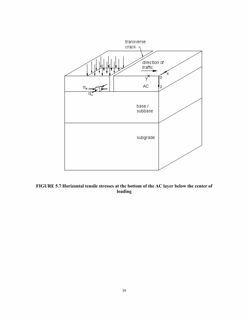
FIGURE 5.7 Horizontal tensile stresses at the bottom of the AC layer below the center of loading
39

FIGURE 5.8 Vertical normal stresses in the base below the center of loading and below the edge of the transverse crack
In the analysis presented in this thesis, the location of the transverse crack was taken directly in front of the loaded area. This location was chosen because it is expected to be the most detrimental to the pavement. In fact, the pavement should experience the highest stresses and largest displacements when the load is positioned at the edge of the crack. Furthermore, only the effect of a fully open crack passing through the full-depth of the AC was investigated. A closed or partly closed frictional crack, considered by Uddin et al. (12) and Uddin and Pan (13) using special GAPUNI elements available in ABAQUS, should produce changes in stresses with respect to uncracked pavement that are less drastic than an open crack.
There are two types of loading induced by a truck tire, local and global, which can be considered in analyzing the pavement response. Local refers to tractions (normal and tangential surface stresses) the individual tire treads transmit onto the pavement. Local tractions play a crucial role in evaluating horizontal stresses next to the AC top surface; such evaluation provides information for analyzing the potential of top-down (longitudinal) cracking. However, when analyzing the effect of transverse cracks on the stress at the bottom of the AC layer and in the base, the distribution of local tractions can be replaced by a statically equivalent global 40

distribution of tractions. The latter is obtained by appropriate averaging procedure of local tractions.
The choice of the specific global tractions distribution was motivated by recent results of physical experiments performed by Pottinger and McIntyre (29) with a truck tire. Pottinger found that besides normal tractions, each tire tread transmits varying tangential tractions (Fig. 5.9). However, when averaged linearly over the whole width of the tire, the magnitude of the tangential tractions becomes negligibly small.
FIGURE 5.9 Shear tractions distribution for truck tire (after Pottinger and McIntyre)
Accordingly, only the presence of uniform normal tractions (pressure) exerted by the tire footprint was considered in the computations. The shape of the footprint was taken as square, as reported in Pottinger and McIntyre (29), and the intensity of uniform pressure as 0.7 MPa (100 psi).
41

42

CHAPTER 6 - Numerical Results
6.1 Longitudinal cracks
6.1.1 Surface stresses due to unit tractions
The computed variation of the horizontal stress σxx perpendicular to the tread across the mid-plane for different AC thickness and uniform σn = 1 MPa is shown in Fig. 6.1. For the most part, increasing the thickness of the AC layer changes the sign of σxx next to the edge of the tread from compression to tension; the distribution of σxx becomes closer to that for the half-space. However, for a very thin AC layer, and due to global bending of the layer, noticeable tensile stresses ≅ 0.01 MPa (1.45 psi) develop at some distance from the edge. Inspection of stresses σxx at other than mid-plane sections revealed slightly higher tension close to the tread's end. This occurs for thick AC layers, and can be explained by noting that mid-plane conditions resemble plane strain, where σxx assumes zero-value outside the loaded area (39). At the end of the tread, conditions are closer to axisymmetric, with non-zero stresses σxx outside the loaded area (39).
The distribution of σxx due to antisymmetric distribution of τn with 1 MPa (145 psi) maximum is shown in Fig. 6.2. Maximum tension occurs at the center of the tread, and the thickness of the AC layer has no effect on stresses. A small effect of the AC layer thickness on σxx is noted for τn acting uni-directionally, with high tension at the edge opposite to the direction of τn, Fig. 6.3.
43
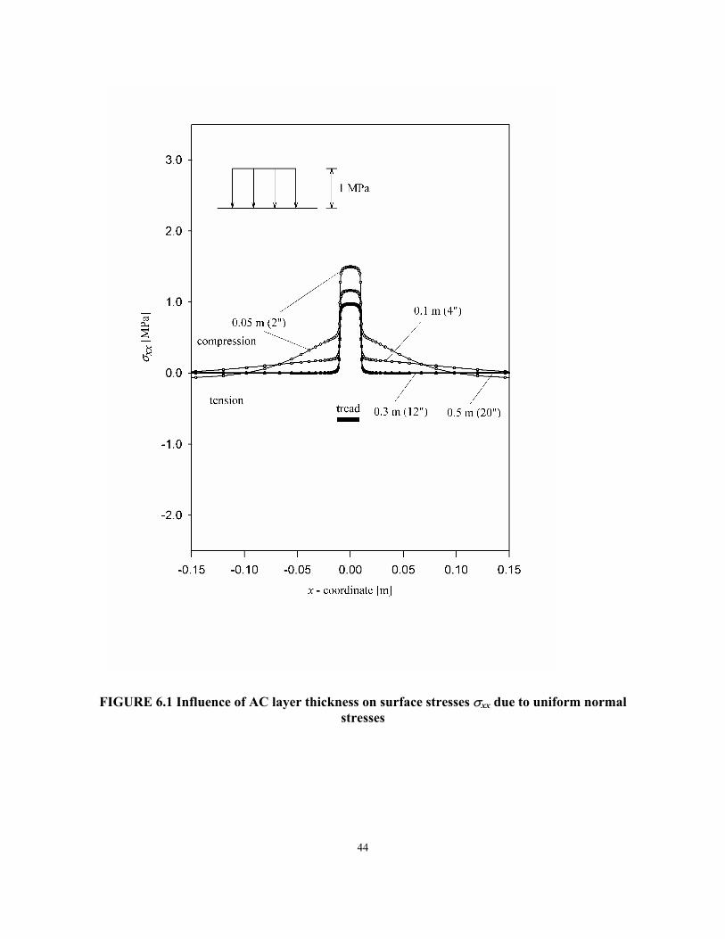
FIGURE 6.1 Influence of AC layer thickness on surface stresses σxx due to uniform normal stresses
44

1s
FIGURE 6.2 Influence of AC layer thickness on surface stresses σxx due to antisymmetric, outward shear stresses
45

s
1
FIGURE 6.3 Influence of AC layer thickness on surface stresses σxx due to uni-directional shear stresses
46

6.1.2 Surface stresses induced by tires
Using superposition and appropriate scaling, the results above were used to determine the normal stresses σxx due both to σn and τn for the central and outermost treads of tires tested by Pottinger and McIntyre (29), and for the AC layer thickness of 0.3 m (12 in.). For the outermost truck tire tread where the contact width was very small (Fig. 5.1a and c), additional ABAQUS computations were performed for the tread width of 0.005 m (0.2 in.). In arriving at the scaling factors, approximate global static equivalence of the loads transmitted by each tread on the pavement was used. Specifically, the distributions of σn were taken as constant, and the distributions of τn as linear; in either case, the integrals of the distributions were equal to those of the distributions reported in (29). The results are shown in Fig. 6.4 and Fig. 6.5.
Clearly, for both tires, no tensile stresses σxx develop within the loaded area of the central tread, Fig. 6.4a and 6.5a. The reason for that is the dominance of compressive stresses σxx induced by tractions σn over tensile stresses σxx induced by tractions τn distributed antisymmetrically with zero-value at the middle. Note that postulating a jump in τn at the center of the tread (6) would produce infinite tension that is not supported by contact mechanics solutions. Outside the loaded area, the stresses σxx still are compressive, but their magnitude is very small.
Significant tension develops outside of the loaded area for the outermost treads in truck and performance tires, as the unidirectional tangential tractions amplify the effect of normal tractions, Fig. 6.4b and 6.5b. The magnitude of tensile stress σxx is greater for performance tire because the total transmitted tangential force is greater than in the truck tire, where the contact area of shoulder tread is narrow. To assess the contribution of all treads on a tire on the surface stresses σxx, Fig. 6.6 and 6.7 representing half of the tire width were constructed. Fig. 6.6 and 6.7 also show the assumed distribution of σn and τn along the tire width, where again approximate static equivalence was used to match the experimental results. When comparing Fig. 6.6 and 6.7, it becomes evident that tensile stresses only develop outside the outermost treads, and their magnitude is greater for the passenger tire. This surprising result can be attributed to the pneumatic effect in the passenger tire tested by Pottinger and McIntyre (29), and should not be extended on other types of tires. It is also apparent that the contributions of neighboring treads are small. This implies that local tread analysis provides sufficiently accurate results for detecting and evaluating tensile surface stresses. Adequate modeling of tractions transmitted by the tread plays here a crucial role.
As mentioned before, the exact value of tractions next to the edge is not known, and increasing the gradient of τn with zero-value at the edge may influenceσxx. To assess this effect, computations were performed for the trapezoidal, uni-directional distribution of τn (Fig. 6.3) with the same slope of the central portion and two different slopes (gradients) at the edge, s = 100 MPa/m and s = 200 MPa/m. The increase in maximum tensile stress σxx amounted to about 20%, which may not be negligible.
47

FIGURE 6.4 Surface stresses σxx for truck tire: (a) central tread,and (b) outermost tread
48

FIGURE 6.5 Surface stresses σxx for passenger tire: (a) central tread and (b) outermost tread
49

FIGURE 6.6 Surface stresses σxx along truck tire width
50
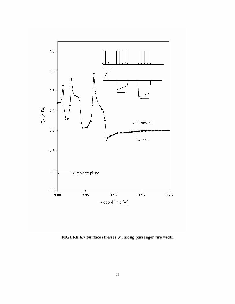
FIGURE 6.7 Surface stresses σxx along passenger tire width
51

6.1.3 Influence of AC layer thickness
From the above analysis, the outermost treads of passenger car tire seem to be more detrimental to AC pavement. Tensile surface stresses developed at some distance away from the loaded area in the thin AC layer. These tensile surface stresses are not due to the uni-directional tangential tractions on the surface, but to global bending of the thin AC layer. On the other hand, significant tensile stresses also developed just outside the outermost treads, as AC layer thickness increases. These tensile stresses are due to the uni-directional tangential tractions on the surface, Fig. 6.8. The maximum surface tensile stresses asymptotically approach the tensile stresses obtained from half-space solution as the AC layer thickness increases, Fig. 6.9.
FIGURE 6.8 Variation of horizontal normal surface stresses σxx
52

FIGURE 6.9 Variation of maximum horizontal normal surface stress σxx
6.2 Transverse cracks
6.2.1 Introduction
Computing 110 cases (55 uncracked, 55 cracked) generated a significant amount of data
that could not be displayed easily. Therefore, the presentation of the results was divided into different sections. Section 6.2.2 presents the distributions of horizontal normal stresses σxx and σyy along the top and bottom of the AC layer for a select number of cases. Section 6.2.3 contains simplified illustrations that present the most important stress data at certain locations for chosen cases. Section 6.2.4 presents the results concerning the influence of material properties (different seasons) on stresses in the AC layer as well as in the base layer. The next section, 6.2.5, addresses how the layer thickness influences the stress in the AC layer and the base layer. Section 6.2.6 presents graphs which summarize the influence of material properties, as well as layer thickness on stresses in the AC layer and base layer. Section 6.2.7 presents the results concerning the influence of transverse cracks have on surface stresses that are of interest in analyzing top-down cracks. 53

6.2.2 Stress distributions The stresses σyy (in the horizontal direction perpendicular to the crack) and σxx (in the horizontal direction parallel to the crack) along the top and bottom of the AC layer, respectively, were extracted from ABAQUS/CAE. These were then used to create graphs to illustrate how a transverse crack affects the stresses along the entire cross section through the center of loading of the pavement. Each of the 110 cases has four graphs: (1) stress σyy along the top of the AC layer, (2) stress σxx along the top of the AC layer, (3) stress σyy along the bottom of the AC layer, and (4) stress σxx along the bottom of the AC layer. Graphed on each plot are the stress distribution for an uncracked pavement (represented by the solid line) and the stress distribution for a pavement with a transverse crack present (represented by a dotted line). The scale for the horizontal axis for each graph remains the same. In each plot the vertical axis has the same scale. In other words, the vertical scale for all of the stress σxx and σyy distributions is the same. Stress distributions for four extreme cases were selected for presentation in this thesis. Figures 6.10 to 6.13 depict the stress distributions for a thin, 0.1 m (4 in.) AC layer, 0.076 m (3 in.) base, and 1.42 m (56 in.) sand subgrade with material properties representing summer conditions (case 3) and winter conditions (case 5). Figures 6.14 to 6.17 present the stress distributions for a thick, 0.3 m (12 in.) AC layer, 0.076 m base, and 1.22 m (48 in.) sand subgrade with material properties representing summer conditions (case 13) and winter conditions (case 15).
54

(a)
(b)
FIGURE 6.10 Horizontal stresses along top of AC layer for AC = 0.1 m (Case 3): (a) stress σyy – perpendicular to crack and (b) stress σxx – parallel to crack
55

(a)
(b)
FIGURE 6.11 Horizontal stresses along bottom of AC layer for AC = 0.1 m (Case 3): (a) stress σyy – perpendicular to crack and (b) stress σxx – parallel to crack
56

(a)
(b)
FIGURE 6.12 Horizontal stresses along top of AC layer for AC = 0.1 m (Case 5): (a) stress σyy – perpendicular to crack and (b) stress σxx – parallel to crack
57
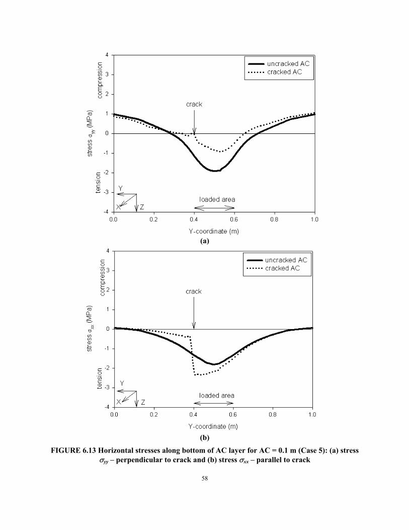
(a)
(b)
FIGURE 6.13 Horizontal stresses along bottom of AC layer for AC = 0.1 m (Case 5): (a) stress σyy – perpendicular to crack and (b) stress σxx – parallel to crack
58
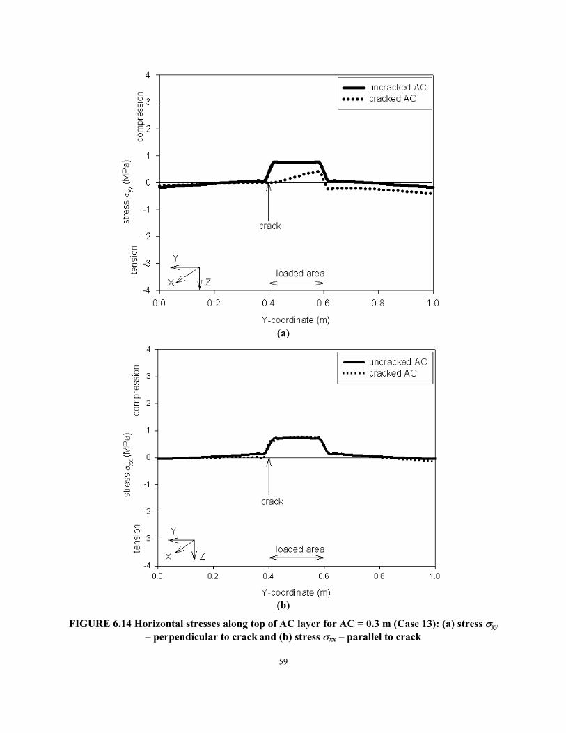
(a)
(b)
FIGURE 6.14 Horizontal stresses along top of AC layer for AC = 0.3 m (Case 13): (a) stress σyy – perpendicular to crack and (b) stress σxx – parallel to crack
59

(a)
(b)
FIGURE 6.16 Horizontal stresses along top of AC layer for AC = 0.3 m (Case 15): (a) stress σyy – perpendicular to crack and (b) stress σxx – parallel to crack
61
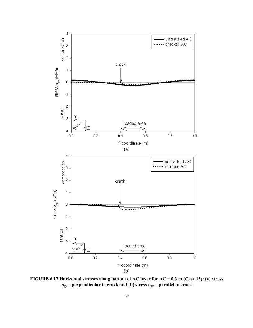
(a)
(b)
FIGURE 6.17 Horizontal stresses along bottom of AC layer for AC = 0.3 m (Case 15): (a) stress σyy – perpendicular to crack and (b) stress σxx – parallel to crack
62

From the results it is observed in general that the magnitude of stress σyy along both the top (compressive) and bottom (tensile) of the AC layer decrease when a transverse crack is present. Conversely, stresses σxx along the top and bottom of the AC layer are increased when a transverse crack is present. Documentation of the stress distributions for all 55 cases can be found on the accompanying CD.
The vertical stresses σzz were only determined at selected locations; therefore, no stress distributions are presented.
6.2.3 Summary cross sections
To present the results in a form readily indicative of the transverse crack effect on the stresses at specific points, summary cross sections were constructed. They show the geometry and material properties for a given case, as well as the magnitude of σxx, σyy, and σzz. The location of the specific point chosen for stress σxx and σyy is below the center of loading at the bottom of the AC layer. There are two specific locations where the magnitude of σzz is reported. The first point is below the center of loading in the base layer. The second point is located below the edge of the transverse crack in the base layer.
In addition to presenting stress values, the effect of transverse cracks on normal stresses in a given direction was quantified by the crack/no crack (stress) ratio CNR defined as
pavementuncrackedaninstresspavementcrackedainstress
CNR =
with CNR = 1 when there is no change in stresses. Four summary cross sections are presented (Figs. 6.18 to 6.21) for the four extreme cases described in Section 6.2.2.
In accordance with the stress distributions described in Section 6.2.2, it is observed that the magnitude of stress σyy along both the top (compressive) and bottom (tensile) of the AC layer decrease when a transverse crack is present. Beneath the center of loading, the corresponding CNR ranges from 0.3 to 0.7. Conversely, stresses σxx along the top and bottom of the AC layer are increased when a transverse crack is present, with the CNR from 1.0 to 1.8. The results also indicate that the compressive vertical stress σzz at the edge of the transverse crack in the base layer is magnified significantly when a transverse crack is present; the CNR reaches up to 36. However, only moderate increase in σzz is observed below the center of loading, CNR about 1.6 to 2.7.
Entire documentation of the summary cross sections for all 55 cases can be found in Appendix C.
6.2.4 Influence of material properties The influence of the five different seasons, or different material properties, was also investigated. The graphs constructed show the magnitude of the stresses σxx and σyy in a thin AC layer (AC = 0.1 m, 4 in.) and a thick AC layer (AC = 0.3 m, 12 in.) directly below the center of loading in an uncracked and in a cracked pavement at a specific location. 63

Each plot contains five cases with different material properties representing five different seasons (early spring, late spring, summer, fall, and winter), but the same geometry. Graphed on each plot are five points representing the five different cases for an uncracked pavement (represented by an open circle connected by a dotted line) and for a cracked pavement (represented by a filled circle connected by a solid line). The scale for the horizontal and vertical axes for each graph remains the same. Figures 6.22 and 6.23 illustrate the results.
64

(a)
(b)
FIGURE 6.15 Horizontal stresses along bottom of AC layer for AC = 0.3 m (Case 13): (a) stress σyy – perpendicular to crack and (b) stress σxx – parallel to crack
60

FIGURE 6.18 Summary cross section for case 3, AC = 0.1 m, base = 0.076 m, and sand subgrade = 1.42 m (C – stress in cracked pavement, NC – stress in pavement with no crack, CNR – crack/no crack (stress) ratio)
65
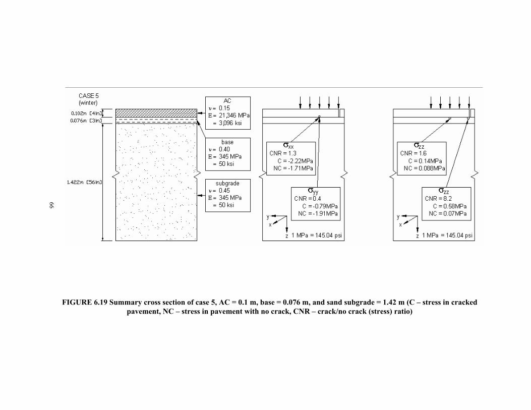
FIGURE 6.19 Summary cross section of case 5, AC = 0.1 m, base = 0.076 m, and sand subgrade = 1.42 m (C – stress in cracked pavement, NC – stress in pavement with no crack, CNR – crack/no crack (stress) ratio)
66

FIGURE 6.20 Summary cross section for case 13, AC = 0.3 m, base = 0.076 m, and sand subgrade = 1.22 m (C – stress in cracked pavement, NC – stress in pavement with no crack, CNR – crack/no crack (stress) ratio)
67

FIGURE 6.21 Summary cross section for case 15, AC = 0.3 m, base = 0.076 m, and sand subgrade = 1.22 m (C – stress in cracked pavement, NC – stress in pavement with no crack, CNR – crack/no crack (stress) ratio)
68

(a)
(b)
FIGURE 6.22 Seasonal horizontal stress variations for cases 1-5, AC = 0.1 m: (a) stress σyy – perpendicular to crack and (b) stress σxx – parallel to crack
69
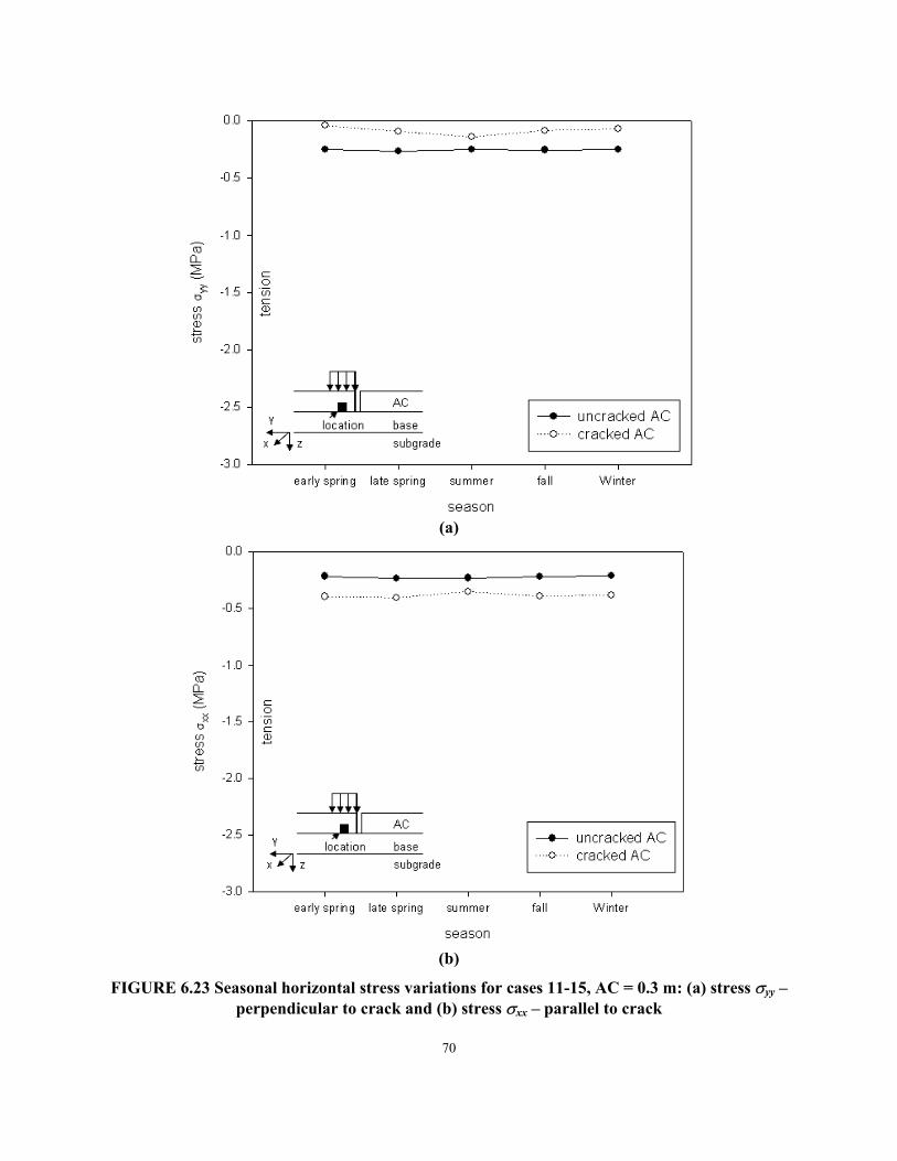
(a)
(b)
FIGURE 6.23 Seasonal horizontal stress variations for cases 11-15, AC = 0.3 m: (a) stress σyy – perpendicular to crack and (b) stress σxx – parallel to crack
70

It is observed once again that the magnitude of the tensile stress σxx increases for all five seasons when a transverse crack is present. The greatest increase takes place in cold seasons (winter and early spring) when the Young’s modulus of AC attains the highest value. In summer, when the Young’s modulus value is low, insignificant change is observed in the magnitude of stress σxx. The opposite effect pertains to the magnitude of the tensile stress σyy, as it decreases for all five seasons when a transverse crack is present. The largest decrease in magnitude is observed in cold seasons, and it is very small in summer.
The seasonal effect on the vertical compressive stress, σzz, in the base is illustrated in Figures 6.24 and 6.25. It is seen that the vertical stress in the base at the edge of the transverse crack is greatly amplified for all five seasons when a transverse crack is present. The greatest increase in magnitude is observed when summer material properties are assigned to the pavement structure. The vertical stress in the base below the center of loading was only slightly increased.
Full documentation of the seasonal stress variation graphs can be found on the accompanying CD.
71

(a)
(b)
FIGURE 6.24 Seasonal vertical stress variations for cases 1-5, AC = 0.1 m: (a) stress σzz below edge of crack in base and (b) stress σzz below center of loading in base
72

(a)
(b)
FIGURE 6.25 Seasonal vertical stress variations for cases 11-15, AC = 0.3 m: (a) stress σzz below edge of crack in base and (b) stress σzz below center of loading in base
73
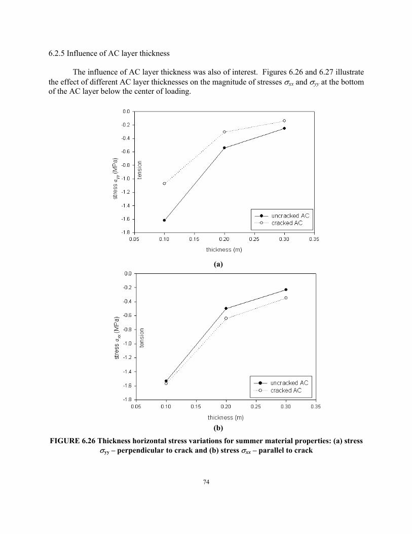
6.2.5 Influence of AC layer thickness The influence of AC layer thickness was also of interest. Figures 6.26 and 6.27 illustrate the effect of different AC layer thicknesses on the magnitude of stresses σxx and σyy at the bottom of the AC layer below the center of loading.
(a)
(b)
FIGURE 6.26 Thickness horizontal stress variations for summer material properties: (a) stress σyy – perpendicular to crack and (b) stress σxx – parallel to crack
74
Each plot contains three cases with different AC layer thicknesses, but the same material properties. Graphed on each plot are three points representing the three different cases for an uncracked pavement (represented by an open circle connected by a dotted line) and for a cracked pavement (represented by a filled circle connected by a solid line). The cases graphed in Figure 6.26 have material properties representing summer conditions, whereas the cases graphed in Figure 6.27 have material properties representing winter conditions. The scale of each graph horizontal axis remains the same. In each plot for a given stress, the vertical axis has the same scale.
It is observed that stress σxx decreases as the thickness of the AC layer increases, when a transverse crack is present. This same trend is observed when a crack is not present, as well. Overall, the magnitude of stress σxx in the cracked AC layer is greater than the magnitude of σxx in the uncracked AC layer. The stress σyy also exhibits the same trend of decreasing in magnitude as the thickness of the AC layer increases for both cracked and uncracked pavement. However, the magnitude of σyy in a cracked AC layer is less than σyy in an uncracked AC layer.
Full documentation of the influence of AC layer thickness graphs can be found on the accompanying CD.
Figures 6.28 and 6.29 illustrate the effect of different AC layer thicknesses on the magnitude of σzz below the edge of the transverse crack in the base, as well as below the center of loading in the base. The cases illustrated in Figure 6.28 have summer material properties whereas the cases presented in Figure 6.29 have winter material properties. The stress σzz both below the edge of the crack in the base, as well as below its center of loading, exhibits the same trend of decreasing in magnitude as the thickness of the AC layer increases for both cracked and uncracked pavement. The magnitude of the stress σzz in the cracked AC layer both below the edge of the crack in the base and below the center of loading in the base is greater than the magnitude of σzz in an uncracked AC layer.
75
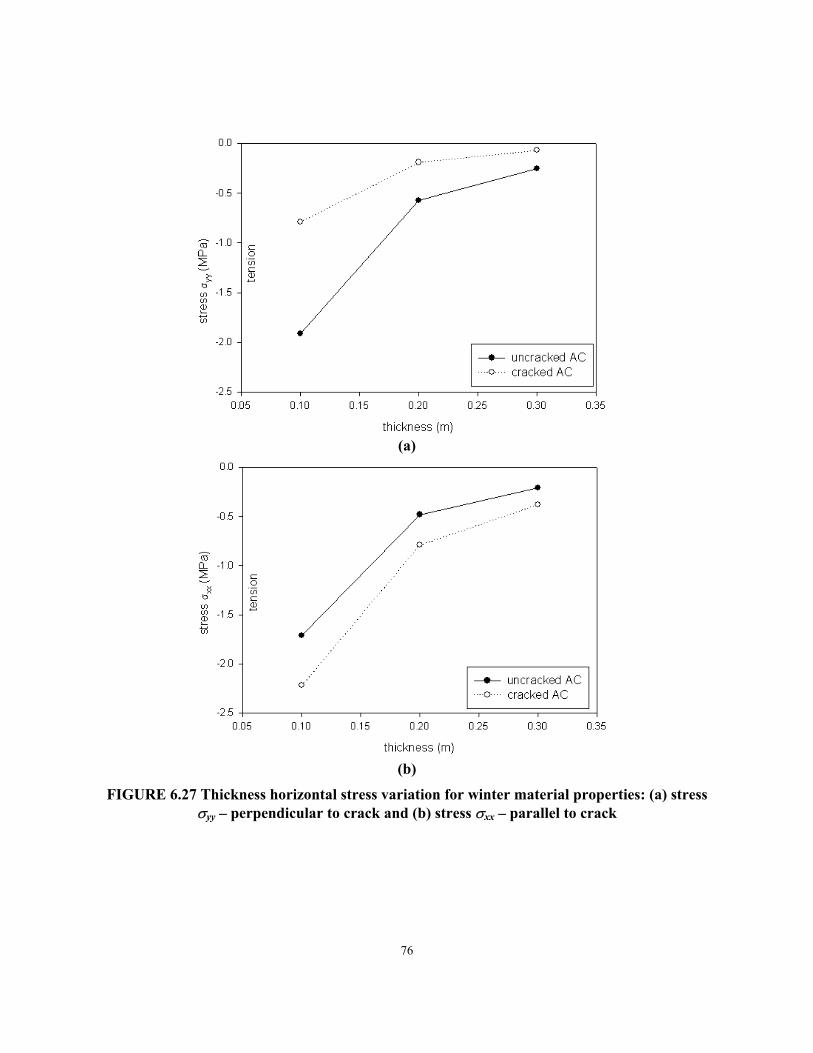
(a)
(b)
FIGURE 6.27 Thickness horizontal stress variation for winter material properties: (a) stress σyy – perpendicular to crack and (b) stress σxx – parallel to crack
76

(a)
(b)
FIGURE 6.28 Thickness vertical stress variations for summer material properties: (a) stress σzz below edge of crack in base and (b) stress σzz below center of loading in base
77

(a)
(b)
FIGURE 6.29 Thickness vertical stress variations for winter material properties: (a) stress σzz below edge of crack in base and (b) stress σzz below center of loading in base
78

6.2.6 CNR line graphs CNR line graphs are alternative illustrations of how the stresses change when a transverse crack is present. In these plots, the coordinates of points represent the stresses in the absence and presence of transverse cracks, and the radial lines correspond to a constant CNR value. The farther away the point is from the CNR = 1 diagonal line, the greater the change in stresses. Letters A and C define regions representing an increase in stresses (either compressive or tensile) due to the presence of crack, and letters B and D regions in decrease in stresses. As, in general, an increase in stresses is detrimental to pavements, regions A and C represent undesirable changes, and regions B and D changes that may be beneficial. Each plot contains 10 or 15 different cases varying either in geometry or material properties. Each case is referred to by case number. The corresponding geometry and material properties can be found in Appendix A. Three CNR line graphs are created for these 10 cases. Figures 6.30, 6.33, 6.36, and 6.39 illustrate the change in horizontal stress σyy, whereas Figures 6.31, 6.34, 6.37, and 6.40 illustrate the change in horizontal stress σxx. Figures 6.32, 6.35, 6.38, and 6.41 illustrate the change in vertical stress σzz below the edge of the transverse crack in the base.
79

FIGURE 6.30 Change in horizontal stress σyy (perpendicular to crack) at the bottom of the AC layer below the center of loading for cases 1-15
80

FIGURE 6.31 Change in horizontal stress σxx (parallel to crack) at the bottom of the AC layer below the center of loading for cases 1-15
81

FIGURE 6.32 Change in vertical stress σzz in the base below the edge of the transverse crack for cases 1-15
82

FIGURE 6.33 Change in horizontal stress σyy (perpendicular to crack) at the bottom of the AC layer below the center of loading for cases 16-30
83
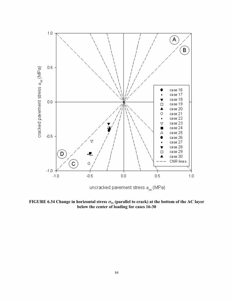
FIGURE 6.34 Change in horizontal stress σxx (parallel to crack) at the bottom of the AC layer below the center of loading for cases 16-30
84

FIGURE 6.35 Change in vertical stress σzz in the base below edge of transverse crack for case 16-30
85

FIGURE 6.36 Change in horizontal stress σyy (perpendicular to crack) at the bottom of the AC layer below the center of loading for cases 31-45
86

FIGURE 6.37 Change in horizontal stress σxx (parallel to crack) at the bottom of the AC layer below the center of loading for cases 31-45
87

FIGURE 6.38 Change in vertical stress σzz in the base below the edge of the transverse crack for cases 31-45
88

FIGURE 6.39 Change in horizontal stress σyy (perpendicular to crack) at the bottom of the AC layer below the center of loading for cases 46-55
89

FIGURE 6.40 Change in horizontal stress σxx (parallel to crack) at the bottom of the AC layer below the center of loading for cases 46-55
90
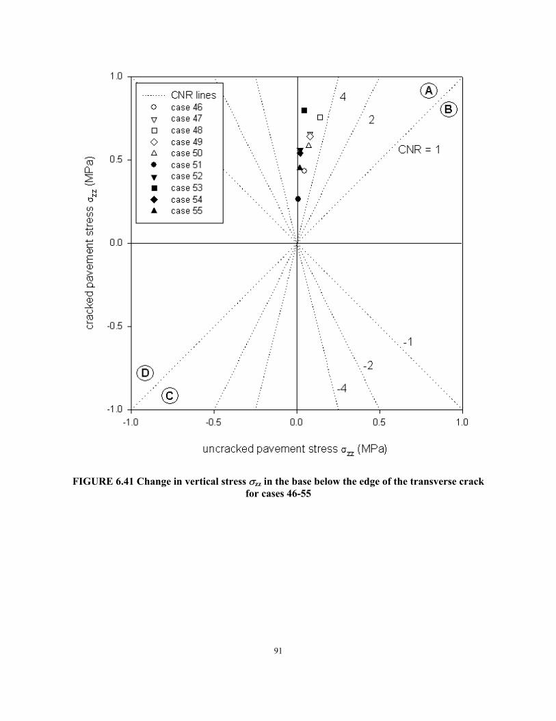
FIGURE 6.41 Change in vertical stress σzz in the base below the edge of the transverse crack for cases 46-55
91

Clearly, the changes at the bottom of the AC layer in the horizontal stresses parallel to the crack are greater than in stresses perpendicular to the crack. The presence of a transverse crack increased the vertical compressive stresses in the base both below the edge of the transverse crack as well as below the center of loading.
6.2.7 Surface stress related to top-down cracking The distributions of stress σxx along the edge of the transverse crack and through the center of loading were used to examine the effect that a transverse crack had on the tensile stresses in the vicinity of the loaded area. Figures 6.42 to 6.45 illustrate the stress distribution σxx (in the horizontal x-direction parallel to the transverse crack) along the edge of the transverse crack, as well as through the center of loading on the surface of the AC layer. Results for a thin AC layer (AC = 0.1 m) for both summer and winter material properties as well as for a thick AC layer (AC = 0.3 m) for both summer and winter material properties, are presented. Each plot is for one specific case of material properties and pavement geometry. Graphed on each plot are the stress distribution for an uncracked pavement (represented by the solid line) and the stress distribution for a pavement with a transverse crack present (represented by a dotted line). The scale for the horizontal and vertical axes for each graph remains the same.
92

(a)
(b)
FIGURE 6.42 Horizontal stresses along top of AC layer for case 3 (AC = 0.1 m, summer material properties): (a) stress σxx through center of loading and (b) stress σxx along the edge of
the transverse crack 93

(a)
(b)
FIGURE 6.43 Horizontal stresses along top of AC layer for case 5 (AC = 0.1 m, winter material properties): (a) stress σxx through center of loading and (b) stress σxx along the edge of the
transverse crack 94

(a)
(b)
FIGURE 6.44 Horizontal stresses along top of AC layer for case 13 (AC = 0.3 m, summer material properties): (a) stress σxx through center of loading and (b) stress σxx along the edge of
the transverse crack 95

(a)
(b)
FIGURE 6.45 Horizontal stresses distribution along top of AC layer for case 15 (AC = 0.3 m, winter material properties): (a) stress σxx through center of loading and (b) stress σxx along the
edge of the transverse crack 96

It is observed from the results that the tensile stress σxx increases when a transverse crack
is present. More specifically, the stress distribution through the center of loading when a transverse crack is present displays a greater increase than along the edge of the transverse crack. This implies that there is a greater potential for the occurrence of surface longitudinal cracks if the pavement contains transverse cracks.
97

98

Chapter 7: Closing Remarks and Conclusions
As stated previously in this report, there were two specific goals of this research project. The conclusions that follow are separated into two sections to address the two different goals.
7.1 Surface stresses in pavement structures
7.1.1 Conclusions derived from contact mechanics
It has been demonstrated in this work that contact mechanics provides valuable information on assigning value and sign to surface tractions in evaluating the tensile surface stresses induced in flexible pavement systems by wheel loads. This is critical when the experiments do not provide details of traction distribution, e.g., next to the edge of the tread. When the assumed distributions disregard the results derived from contact mechanics the corresponding numerical results may be grossly in error.
In particular, the normal and tangential tractions at the edge of the loaded area (tread) are of zero-value even though their gradient may be very high. If the tread is loaded only vertically, the tangential tractions are distributed antisymmetrically, outward, and have zero-value in the middle. If the load is inclined, as is the case with outer treads in pneumatic tires, the tangential tractions may act uni-directionally towards the center of the tire patch.
The distribution of normal tractions has no qualitative effect on horizontal surface stresses, which remain finite even if a jump of normal tractions is postulated at the tread edge. On the other hand, assuming a finite-value jump in tangential tractions, whether at the tread edge or at another location, leads to locally infinite horizontal surface stresses. As the latter is also unaffected by the thickness of the AC layer, inaccurate results may be obtained when a jump in tangential tractions is postulated.
7.1.2 Conclusions derived from numerical simulations
Numerical computations using ABAQUS for a specific rectangular loaded area simulating a tire tread, and for tractions with unit maximum magnitude, reveal the following observations:
1. The normal tractions induce horizontal stresses that are compressive within the loaded area and compressive/tensile outside the area. The location of tensile stresses and their magnitude depends on the thickness of the AC layer. In a very thin layer (0.05 m), the stresses become tensile at a distance of about five-times the width of the loaded area. With increasing thickness, maximum tensile stresses first are located further away and then closer to the edge of the area.
2. Antisymmetric tangential tractions pointing outward induce tensile stresses within the loaded
area and compressive stresses outside the area. This is unaffected by the AC layer thickness.
99

3. Uni-directional tangential tractions induce tensile surface stresses on the side opposite to the direction of tractions; on the other side, the stresses are compressive.
Computations using the loads reported by Pottinger and McIntyre (29) for the truck and passenger performance tires show that 4. For both types of tires, the wheel load transmitted through the inner treads induces high
horizontal compressive stresses within the loaded area, and small compressive stresses outside the area.
5. The load transmitted through the outer treads in truck and passenger tires induces high
compressive surface stresses within the loaded area and smaller but significant tensile stresses outside the tires.
6. The horizontal surface tension stress outside the outermost tire tread increases as the
thickness of AC layer increases. This tension will asymptotically reach a value similar to the one obtained from half-space solution.
7. The distribution of horizontal surface stresses for the whole tire is not much different from
distributions for individual treads; the effect of superposition is small. This implies that local analysis provides the important information on the sign and magnitude of horizontal surface stress.
8. It is observed from the results that the tensile stress σxx increases when a transverse crack is
present in a thin AC layer. The increase in the tensile stress σxx is negligible in a thick AC layer. This implies that there is a greater potential for the occurrence of surface longitudinal cracks if the AC pavement is thin and contains transverse cracks.
7.1.3 Remarks
Some of the findings above are case-specific in that they apply to tires and loads reported by Pottinger and McIntyre (29). Nonetheless, some general comments seem appropriate.
As the uni-directional tangential tractions induced at outer treads appear to be the main reason for tensile surface stresses, attention should focus on conducting tests and gathering data on their magnitude and distribution.
The computations indicated very high gradients of surface stresses next to the edge of the loaded areas (treads). Their effect on asphalt concrete failure is unclear. Also, a fuller analysis of all stress components should be conducted to investigate the possibility of high shear stresses.
Contact mechanics solutions indicate slip next to the edge of contact. This may result in fretting, the phenomenon of surface failure due to repeated local slip. Analyzing this phenomenon as a potential cause for top-down cracking seems intriguing.
It appears that the progress in analyzing top-down cracking will be slow unless future research focuses on the effect of tire geometry and the resulting loads on the surface stresses in AC layers. Cooperation with tire manufacturers plays here a crucial role. 100

7.2 Influence of transverse cracking on stresses in pavement structures
7.2.1 Conclusions
Numerical computations using ABAQUS provided information on normal stresses induced by a single wheel load (pressure) located next to a fully open transverse crack in flexible pavements with and without the presence of transverse (thermal) cracks. Conclusions that can be drawn from this research follow:
1. With the wheel load located next to a fully open transverse crack, there is noticeable
change in horizontal and vertical normal stresses in the asphalt concrete and in the base. This change occurs regardless of the thickness and properties of individual layers.
2. Beneath the center of the wheel load, the magnitude of the horizontal compressive normal stresses σyy in the direction perpendicular to the crack decrease at the top of the AC layer. The magnitude of the horizontal tensile normal stresses σyy in the direction perpendicular to the crack at the bottom of the AC layer also decreases. However, the magnitude of the normal stresses σxx at these locations increases in the direction parallel to the crack. Both changes are moderate and depend on asphalt concrete layer thickness and layer properties.
3. The vertical stresses in the base next to the asphalt concrete layer increase in the presence of transverse crack. Significant increase in vertical stresses takes place next to the bottom of the crack. A much smaller increase occurs beneath the center of the wheel load in the base away from the crack.
4. Overall, the magnitude of the horizontal tensile stress σyy at the bottom of the AC layer perpendicular to the crack decreases for all five seasons (different material properties). The most noticeable change in magnitude of stress σyy occurs during the seasons of early spring and winter. On the other hand, the magnitude of the horizontal tensile stress σxx at the bottom of the AC layer parallel to the crack increases for all five seasons. Once again, the most noticeable change in magnitude of stress σxx occurs during the seasons of early spring and winter. The vertical compressive stress in the base increases for all five seasons. A greater increase in magnitude is observed closer to the transverse crack in the base than in the base below the center of loading.
5. As the thickness of the AC layer increases, the magnitude of the stress (both σyy and σxx) decrease. This trend is observed in both uncracked and cracked pavement. The magnitude of the horizontal normal stress σyy at the bottom of the AC layer decreases for all AC layer thicknesses when a crack is present. Conversely, the magnitude of the horizontal normal stress σxx at the bottom of the AC layer increases for all AC layer thicknesses when a crack is present.
101

7.2.2 Remarks The necessity of modeling the pavement system three-dimensionally came because the change in the stress σxx, which is parallel to the crack, cannot be recovered using two-dimensional or plane-strain modeling. Employing an axisymmetric model does not allow for incorporating a transverse crack into the analysis.
Presenting the results of this research in a useful and easy-to-understand way was challenging, both because the problem was modeled three-dimensionally and because of the large number of cases that had to be computed. The amount of data generated was enormous. To report the results in a tabulated form was nearly impossible, as well as useless. Instead, various plots and illustrations were generated. Of the many possible ways to present the results, these plots and illustrations were deemed to be logical and useful. Due to the large number of graphs created, it was impossible to include all of the graphs within this report. The complete record of all computations is provided on a CD that accompanies this report. This CD contains the ABAQUS *.cae file, as well as the raw data for the stress distributions, material (seasons) variation graphs, and thickness variation graphs for each case.
It is recommended that future research concentrates on improving the modeling of the base and subgrade layers. In particular, elasto-plastic rather than elastic models should be considered, which capture the mechanical properties of these materials adequately. In fact, the high vertical stresses found in the base layer beneath the transverse crack may cause plastic yielding of the material. This phenomenon cannot be described by the elastic model. Testing the plastic (strength) properties of base and subgrade materials seems here mandatory for arriving at numerical values of the relevant parameters that are needed in numerical simulations.
102
References
1. MnPave Flexible Pavement Design Beta v5.010, Computer Shareware by B. Chadbourn, J. Siekmeier, S. Dai, D. Van Deusen, P. Davich, and B. Hoefer, Minnesota Department of Transportation, 2000-2001.
2. A. Collop and D. Cebon, “A Theoretical Analysis of Fatigue Cracking in Flexible Pavements,” Proceedings of the Institution of Mechanical Engineers. Part C, vol. 209, no. 5 (1995), 345-361.
3. A. Gerritsen, C.V. Gurp, J. van der Heide, A. Molenaar, and A. Pronk, “Prediction and Prevention of Surface Cracking in Asphaltic Pavements,” Proceedings of the 6th
International Conference on Structural Design of Asphalt Pavements (July 1987), 378-392.
4. M.M.J. Jacobs, A. de Bondt, A.A.A. Molenaar, and P. Hopman, “Cracking in Asphalt Concrete Pavements,” Proceedings of the 7th International Conference on Asphalt Pavements, vol. 1 (1992), 89-105.
5. A.A.A. Molenaar, “Fatigue and Reflection Cracking due to Traffic Loads,” Proceeding of the Association of Asphalt Paving Technologists, vol. 53 (1984), 440-474.
6. L.A. Myers, R. Roque, and B. Ruth, “Mechanisms of Surface-Initiated Longitudinal Wheel Path Cracks in High-Type Bituminous Pavements,” Journal of the Asphalt Paving Technologists, vol. 67 (1998), 401-432.
7. ABAQUS/CAE version 6.2-1, Computer Software for Interactive Finite Element Analysis by Hibbitt, Karlsson & Sorensen, Inc.
8. ABAQUS/STANDARD version 6.2-1, Computer Software for Finite Element Analysis by Hibbitt, Karlsson & Sorensen, Inc.
9. CIRCLY version 2, Computer Program for the Analysis of Multiple Complex Circular Loads on Layered Anisotropic Media by L.J. Wardle, Division of Applied Geomechanics, CSIRO, Australia, 1977.
10. Bitumen Structures Analysis in Roads (BISAR), Computer Program by Koninlikijke/Shell-Laboratorium, Amsterdam, July 1972.
11. A.M. Tabatabaie and E.J. Barenberg, “Finite-Element Analysis of Jointed or Cracked Concrete Pavements,” Transportation Research Record 671, Transporation Research Board (TRB), National Research Council (Washington, D.C., 1978), 11-19.
12. W. Uddin, A.H. Zhang, and F. Fernandez, “Finite Element Simulation of Pavement Discontinuities and Dynamic Load Response,” Transportation Research Record 1448, TRB, National Research Council (Washington D.C., 1994), 100-106.
103

13. W. Uddin and Z. Pan, “Finite Element Analysis of Flexible Pavements with Discontinuities,” Transportation Congress, Proceedings, vol. 1 (1995), 410-423.
14. M. Dauzats and A. Rampal, “Mechanism of Surface Cracking in Wearing Courses,” Proceedings of the 6th International Conference on Structural Design of Asphalt Pavements (1987), 232-247.
15. S. Matsuno and T. Nishizawa, “Mechanism of Longitudinal Surface Cracking in Asphalt Pavement,” Proceedings of 7th International Conference on Asphalt Pavements, vol. 2 (1992), 277-291.
16. A. Bensalem, A.J. Brown, M.E. Nunn, D.B. Merrill, and W.G. Lloyd, “Finite Element Modeling of Fully Flexible Pavement: Surface Cracking and Wheel Interaction,” Proceedings of the 2nd International Symposium on 3D Finite Element for Pavement Analysis, Design, and Research (October 2000), 103-113
17. J.S. Uhlmeyer, K. Willoughby, L.M. Pierce, and J.P. Mahoney, “Top-Down Cracking in Washington State Asphalt Concrete Wearing Courses,” Transportation Research Record 1730, Transportation Research Board (TRB), National Research Council (Washington D.C., 2000), 110-116.
18. Minnesota Department of Transportation, Field Observation Graphs For Longitudinal Surface Cracks (2000).
19. Z. Zhang, R. Roque, and B. Birgisson, “Evaluation of Laboratory Measured Crack Growth Rate for Asphalt Mixtures,” Transportation Research Record 1767, Transportation Research Board (TRB), National Research Council (Washington D.C., 2001), 67-75.
20. A.H.D. Markwick and J.H. Starks, “Stresses Between Tire and Road,” Journal of the Institution of Civil Engineers, vol. 16 (1940-1941), 309-325.
21. N. Seitz and A.W. Hussmann, “Forces and Displacements in Contact Area of Free Rolling Tires,” Society of Automotive Engineers, 710626, Society of Automotive Engineers, Inc. (1971), 1-7.
22. S.A. Lippmann, “Effects of Tire Structure and Operating Conditions on the Distribution of Stress Between the Tread and the Road,” The Tire Pavement Interface, ASTM (Philadelphia, 1985), 91-109.
23. P. Sebaaly and N. Tabatabaee, “Effects of Tire Pressure and Type on Response of Flexible Pavement,” Transportation Research Record 1227, Transportation Research Board (TRB), National Research Council (Washington D.C., 1989), 115-127.
24. M. Huhtala, J. Pihlajamäki, and M. Pienimäki, “Effects of Tires and Tire Pressure on Road Pavements,” Transportation Research Record 1227, Transportation Research Board (TRB), National Research Council (Washington D.C., 1989), 107-114.
104
25. M.G. Pottinger, “The Three-Dimensional Contact Patch Stress Field of Solid and Pneumatic Tires,” Tire Science and Technology, TSTCA, vol. 20, no. 1 (1992), 3-32.
26. J.T. Tielking and M.A. Abraham, “Measurement of Truck Tire Footprint Pressures,” Transportation Research Record 1435, Transportation Research Board (TRB), National Research Council (Washington D.C., 1994), 92-99.
27. M. DeBeer, C. Fisher, and F.J. Jooste, “Determination of Pneumatic Tyre/Pavement Interface Contacts Stresses Under Moving Loads and Some Effects on Pavements with Thin Asphalt Surfacing Layers,” Proceeding of the 8th International Conference on Asphalt Pavements, vol. 1 (1997), 179-227.
28. L.A. Myers, R. Roque, B.E. Ruth, and C. Drakos, “Measurement of Contact Stresses for Different Truck Types to Evaluate Their Influence on Near-Surface Cracking and Rutting,” Transportation Research Record 1655, Transportation Research Board (TRB), National Research Council (Washington D.C., 1999), 175-184.
29. M.G. Pottinger and J.E. McIntyre, “Effects of Suspension Alignment and Modest Cornering on the Footprint Behavior of Performance Tires and Heavy Duty Radial Tires,” Tire Science and Technology, TSTCA, vol. 27, no. 3 (1999), 128-160.
30. D. Perdomo and B. Nokes, “Theoretical Analysis of the Effects of Wide-Base Tires on Flexible Pavement Using CIRCLY,” Transportation Research Record 1388, Transportation Research Board (TRB), National Research Council (Washington D.C., 1993), 108-119.
31. M.M.J. Jacobs, Crack Growth in Asphaltic Mixes, Ph.D. thesis (Delft University of Technology, The Netherlands, 1995).
32. R. Roque, L.A. Myers, and B. Birgisson, “Evaluation of Measured Tire Contact Stresses for the Prediction of Pavement Response and Performance,” Transportation Research Record 1716, Transportation Research Board (TRB), National Research Council (Washington D.C., 2000), 175-184.
33. T. Svasdisant, M. Schorsch, G.Y. Baladi, and S. Pinyosunun, “Mechanistic Analysis of Top-Down Cracks in Asphalt Pavements,” Transportation Research Record, Transportation Research Board (TRB), National Research Council (Washington, D.C., 2002), Paper number: 02-2854.
34. J. Perret, “The Effect of Loading Conditions on Pavement Response Calculated Using a Linear-Elastic Model,” Proceeding of the 3rd International Symposium on 3D Finite Element for Pavement Analysis, Design and Research (2002), 283-303.
35. Y-H Cho, B.F. McCullough, and J. Weissmann, “Considerations on Finite-Element Method Application in Pavement Structural Analysis,” Transportation Research Record 1539, Transportation Research Board (TRB), National Research Council (Washington, D.C., 1996), 96-101.
105

36. H.M. Westergaard, “Computation of Stresses in Concrete Roads,” Proceedings, HRB, vol. 6 (1926), 25-35.
37. G. Pickett and G.K. Ray, “Influence Charts for Concrete Pavements,” Transportation, ASCE, vol. 116 (1951), 49-73.
38. S. Zahgoul and T. White, “Use of Three-Dimensional, Dynamic Finite-Element Program for Analysis of Flexible Pavement,” Transportation Research Record 1388, Transportation Research Board, National Research Council (Washington, D.C., 1993), 60-69.
39. K.L. Johnson, Contact Mechanics (Cambridge: Cambridge University Press, 1985).
40. G.G. Adams and D.B. Bogy, “The Plane Solution for the Elastic Contact Problem of a Semi-Infinite Strip and Half Plane,” Journal of Applied Mechanics, Transactions of the ASME, vol. 43, no. 4 (1976), 603-607.
41. J.P. Dempsey and H. Li, “A Flexible Rectangular Plate on an Elastic Layer: Large Area Contact,” Journal of Tribology, Transactions of the ASME, vol. 111 (1989), 518-524.
42. K.L. Johnson, J.J. O'Connor, and A.C. Woodward, “The Effect of the Indenter Elasticity on the Hertzian Fracture of Brittle Materials,” Proceedings of the Royal Society of London. Series A, Mathematical and Physical Sciences, vol. 334, no. 1596 (1973), 95-117.
43. M.R. Gecit, “Axisymmetric Contact Problem for a Semi-Infinite Cylinder and a Half Space,” International Journal of Engineering Science, vol. 24, no. 8 (1986), 1245-1256.
44. D.A. Spence, “The Hertz Contact Problem with Finite Friction,” Journal of Elasticity, vol. 5, no. 3-4 (1975), 297-319.
45. R.D. Mindlin, “Compliance of Elastic Bodies in Contact,” Journal of Applied Mechanics, Transactions of the ASME, vol. 16, no. 3 (1949), 259-268.
46. E.S. Barber, “Shear Loads on Pavements,” Public Road, A Journal of Highway Research, vol. 32, no. 6 (1963), 141-144.
47. L.A. Myers, R. Roque, and B. Birgisson, “Propagation Mechanisms for Surface-Initiated Longitudinal Wheel Path Cracks,” Transportation Research Record 1778, Transportation Research Board (TRB), National Research Council (Washington D.C., 2001), 113-122.
48. L.A. Myers and R. Roque, “Top-Down Crack Propagation in Bituminous Pavements and Implications for Pavement Management,” Journal of the Asphalt Paving Technologists, in press.
49. H.G. Poulos and E.H. Davis, Elastic Solutions for Soil and Rock Mechanics (New York: John Wiley & Sons, Inc., 1974).
106

107
50. A.E.H. Love, “The Stress Produced in a Semi-Infinite Solid by Pressure on Part of the Boundary,” Philosophical Transactions of the Royal Society of London. Series A, Containing Papers of a Mathematical or Physical Character, vol. 228 (1929), 377-420.
51. W.R. Dean, H.W. Parsons, and I.N. Sneddon, “A Type of Stress Distribution on the Surface of a Semi-Infinite Elastic Solid,” Proceeding of the Cambridge Philosophical Society, vol. 40 (1994), 5-19.
52. Weslea for Windows version 3.0, A Mechanistic Multi-layers Pavement Analysis Computer Program by D. Timm, B. Birgisson, and D. Newcomb, Department of Civil Engineering, University of Minnesota, 1999.
53. C.M. Gerrard and W. J. Harrison, “The Analysis of a Loaded Half Space Comprised of Anisotropic Layers,” CSIRO Aust. Div. Appl. Geomechanics Tech. Pap., no. 10 (1971).
54. L.J. Wardle, “Integral Transform Methods for Multilayered Anisotropic Elastic Systems,” CSIRO Aust. Div. Appl. Geomechanics Tech. Pap., no. 27 (1976).

Appendix A
Simulation Matrix

Appendix A – Simulation matrix CASE 1
(early spring) HMA Base Class 5 Select Granular Sub Grade
Thickness 4 in. (0.1 m) 3 in. (0.076 m) 0 56 in. (1.42 m) Clay loam
Young's modulus 1,647,000 psi (11,356 MPa)
11,000 psi (76 MPa) 0 50,000 psi
(345 MPa)
Poisson's ratio 0.15 0.4 0 0.45
CASE 2 (late spring) HMA Base Class 5 Select Granular Sub Grade
Thickness 4 in. (0.1 m) 3 in. (0.076 m) 0 56 in. (1.42 m) Clay loam
Young's modulus 641,900 psi (4426 MPa)
15,000 psi (104 MPa) 0 5100 psi
(35 MPa)
Poisson's ratio 0.26 0.4 0 0.45
CASE 3 (summer) HMA Base Class 5 Select Granular Sub Grade
Thickness 4 in. (0.1 m) 3 in. (0.076 m) 0 56 in. (1.42 m) Clay loam
Young's modulus 256,100 psi (1766 MPa)
19,000 psi (131 MPa) 0 6200 psi
(43 MPa)
Poisson's ratio 0.38 0.4 0 0.45
CASE 4 (fall) HMA Base Class 5 Select Granular Sub Grade
Thickness 4 in. (0.1 m) 3 in. (0.076 m) 0 56 in. (1.42 m) Clay loam
Young's modulus 974,800 psi (6721 MPa)
22,000 psi (152 MPa) 0 7300 psi
(51 MPa)
Poisson's ratio 0.19 0.4 0 0.45
CASE 5 (winter) HMA Base Class 5 Select Granular Sub Grade
Thickness 4 in. (0.1 m) 3 in. (0.076 m) 0 56 in. (1.42 m) Clay loam
Young's modulus 3,096,000 psi (21,346 MPa)
50,000 psi (345 MPa) 0 50,000 psi
(345 MPa)
Poisson's ratio 0.15 0.4 0 0.45
A-1

CASE 6 (early spring) HMA Base Class 5 Select Granular Sub Grade
Thickness 8 in. (0.2 m) 3 in. (0.076 m) 0 52 in. (1.32 m) Clay loam
Young's modulus 1,647,000 psi (11,356 MPa)
11,000 psi (76 MPa) 0 50,000 psi
(345 MPa)
Poisson's ratio 0.15 0.4 0 0.45
CASE 7
(late spring) HMA Base Class 5 Select Granular Sub Grade
Thickness 8 in. (0.2 m) 3 in. (0.076 m) 0 52 in. (1.32 m) Clay loam
Young's modulus 641,900 psi (4426 MPa)
15,000 psi (104 MPa) 0 5100 psi
(35 MPa)
Poisson's ratio 0.26 0.4 0 0.45
CASE 8
(summer) HMA Base Class 5 Select Granular Sub Grade
Thickness 8 in. (0.2 m) 3 in. (0.076 m) 0 52 in. (1.32 m) Clay loam
Young's modulus 256,100 psi (1766 MPa)
19,000 psi (131 MPa) 0 6200 psi
(43 MPa)
Poisson's ratio 0.38 0.4 0 0.45
CASE 9
(fall) HMA Base Class 5 Select Granular Sub Grade
Thickness 8 in. (0.2 m) 3 in. (0.076 m) 0 52 in. (1.32 m) Clay loam
Young's modulus 974,800 psi (6721 MPa)
22,000 psi (152 MPa) 0 7300 psi
(51 MPa)
Poisson's ratio 0.19 0.4 0 0.45
CASE 10 (winter) HMA Base Class 5 Select Granular Sub Grade
Thickness 8 in. (0.2 m) 3 in. (0.076 m) 0 52 in. (1.32 m) Clay loam
Young's modulus 3,096,000 psi (21,346 MPa)
50,000 psi (345 MPa) 0 50,000 psi
(345 MPa)
Poisson's ratio 0.15 0.4 0 0.45
A-2

CASE 11 (early spring) HMA Base Class 5 Select Granular Sub Grade
Thickness 12 in. (0.3 m) 3 in. (0.076 m) 0 48 in. (1.22 m) Clay loam
Young's modulus 1,647,000 psi (11,356 MPa)
11,000 psi (76 MPa) 0 50,000 psi
(345 MPa)
Poisson's ratio 0.15 0.4 0 0.45
CASE 12
(late spring) HMA Base Class 5 Select Granular Sub Grade
Thickness 12 in. (0.3 m) 3 in. (0.076 m) 0 48 in. (1.22 m) Clay loam
Young's modulus 641,900 psi (4426 MPa)
15,000 psi (104 MPa) 0 5100 psi
(35 MPa)
Poisson's ratio 0.26 0.4 0 0.45
CASE 13 (summer) HMA Base Class 5 Select Granular Sub Grade
Thickness 12 in. (0.3 m) 3 in. (0.076 m) 0 48 in. (1.22 m) Clay loam
Young's modulus 256,100 psi (1766 MPa)
19,000 psi (131 MPa) 0 6200 psi
(43 MPa)
Poisson's ratio 0.38 0.4 0 0.45
CASE 14
(fall) HMA Base Class 5 Select Granular Sub Grade
Thickness 12 in. (0.3 m) 3 in. (0.076 m) 0 48 in. (1.22 m) Clay loam
Young's modulus 974,800 psi (6721 MPa)
22,000 psi (152 MPa) 0 7300 psi
(51 MPa)
Poisson's ratio 0.19 0.4 0 0.45
CASE 15 (winter) HMA Base Class 5 Select Granular Sub Grade
Thickness 12 in. (0.3 m) 3 in. (0.076 m) 0 48 in. (1.22 m) Clay loam
Young's modulus 3,096,000 psi (21,346 MPa)
50,000 psi (345 MPa) 0 50,000 psi
(345 MPa)
Poisson's ratio 0.15 0.4 0 0.45
A-3

CASE 16 (early spring) HMA Base Class 5 Select Granular Sub Grade
Thickness 4 in. (0.1 m) 6 in. (0.15 m) 24 in. (0.6 m) 29 in. (0.75 m) Clay loam
Young's modulus 1,647,000 psi (11,356 MPa)
11,000 psi (76 MPa)
6200 psi (43 MPa)
50,000 psi (345 MPa)
Poisson's ratio 0.15 0.4 0.4 0.45
CASE 17
(late spring) HMA Base Class 5 Select Granular Sub Grade
Thickness 4 in. (0.1 m) 6 in. (0.15 m) 24 in. (0.6 m) 29 in. (0.75 m) Clay loam
Young's modulus 641,900 psi (4426 MPa)
15,000 psi (104 MPa)
8700 psi (60 MPa)
5100 psi (35 MPa)
Poisson's ratio 0.26 0.4 0.4 0.45
CASE 18 (summer) HMA Base Class 5 Select Granular Sub Grade
Thickness 4 in. (0.1 m) 6 in. (0.15 m) 24 in. (0.6 m) 29 in. (0.75 m) Clay loam
Young's modulus 256,100 psi (1766 MPa)
19,000 psi (131 MPa)
10,600 psi (73 MPa)
6200 psi (43 MPa)
Poisson's ratio 0.38 0.4 0.4 0.45
CASE 19
(fall) HMA Base Class 5 Select Granular Sub Grade
Thickness 4 in. (0.1 m) 6 in. (0.15 m) 24 in. (0.6 m) 29 in. (0.75 m) Clay loam
Young's modulus 974,800 psi (6721 MPa)
22,000 psi (152 MPa)
12,400 psi (86 MPa)
7300 psi (51 MPa)
Poisson's ratio 0.19 0.4 0.4 0.45
CASE 20 (winter) HMA Base Class 5 Select Granular Sub Grade
Thickness 4 in. (0.1 m) 6 in. (0.15 m) 24 in. (0.6 m) 29 in. (0.75 m) Clay loam
Young's modulus 3,096,000 psi (21,346 MPa)
50,000 psi (345 MPa)
50,000 psi (345 MPa)
50,000 psi (345 MPa)
Poisson's ratio 0.15 0.4 0.4 0.45
A-4

CASE 21 (early spring) HMA Base Class 5 Select Granular Sub Grade
Thickness 8 in. (0.2 m) 6 in. (0.15 m) 24 in. (0.6 m) 25 in. (0.65 m) Clay loam
Young's modulus 1,647,000 psi (11,356 MPa)
11,000 psi (76 MPa)
6200 psi (43 MPa)
50,000 psi (345 MPa)
Poisson's ratio 0.15 0.4 0.4 0.45
CASE 22
(late spring) HMA Base Class 5 Select Granular Sub Grade
Thickness 8 in. (0.2 m) 6 in. (0.15 m) 24 in. (0.6 m) 25 in. (0.65 m) Clay loam
Young's modulus 641,900 psi (4426 MPa)
15,000 psi (104 MPa)
8700 psi (60 MPa)
5100 psi (35 MPa)
Poisson's ratio 0.26 0.4 0.4 0.45
CASE 23 (summer) HMA Base Class 5 Select Granular Sub Grade
Thickness 8 in. (0.2 m) 6 in. (0.15 m) 24 in. (0.6 m) 25 in. (0.65 m) Clay loam
Young's modulus 256,100 psi (1766 MPa)
19,000 psi (131 MPa)
10,600 psi (73 MPa)
6200 psi (43 MPa)
Poisson's ratio 0.38 0.4 0.4 0.45
CASE 24
(fall) HMA Base Class 5 Select Granular Sub Grade
Thickness 8 in. (0.2 m) 6 in. (0.15 m) 24 in. (0.6 m) 25 in. (0.65 m) Clay loam
Young's modulus 974,800 psi (6721 MPa)
22,000 psi (152 MPa)
12,400 psi (86 MPa)
7300 psi (51 MPa)
Poisson's ratio 0.19 0.4 0.4 0.45
CASE 25 (winter) HMA Base Class 5 Select Granular Sub Grade
Thickness 8 in. (0.2 m) 6 in. (0.15 m) 24 in. (0.6 m) 25 in. (0.65 m) Clay loam
Young's modulus 3,096,000 psi (21,346 MPa)
50,000 psi (345 MPa)
50,000 psi (345 MPa)
50,000 psi (345 MPa)
Poisson's ratio 0.15 0.4 0.4 0.45
A-5

CASE 26 (early spring) HMA Base Class 5 Select Granular Sub Grade
Thickness 12 in. (0.3 m) 6 in. (0.15 m) 24 in. (0.6 m) 21 in. (0.55 m) Clay loam
Young's modulus 1,647,000 psi (11,356 MPa)
11,000 psi (76 MPa)
6200 psi (43 MPa)
50,000 psi (345 MPa)
Poisson's ratio 0.15 0.4 0.4 0.45
CASE 27
(late spring) HMA Base Class 5 Select Granular Sub Grade
Thickness 12 in. (0.3 m) 6 in. (0.15 m) 24 in. (0.6 m) 21 in. (0.55 m) Clay loam
Young's modulus 641,900 psi (4426 MPa)
15,000 psi (104 MPa)
8700 psi (60 MPa)
5100 psi (35 MPa)
Poisson's ratio 0.26 0.4 0.4 0.45
CASE 28 (summer) HMA Base Class 5 Select Granular Sub Grade
Thickness 12 in. (0.3 m) 6 in. (0.15 m) 24 in. (0.6 m) 21 in. (0.55 m) Clay loam
Young's modulus 256,100 psi (1766 MPa)
19,000 psi (131 MPa)
10,600 psi (73 MPa)
6200 psi (43 MPa)
Poisson's ratio 0.38 0.4 0.4 0.45
CASE 29
(fall) HMA Base Class 5 Select Granular Sub Grade
Thickness 12 in. (0.3 m) 6 in. (0.15 m) 24 in. (0.6 m) 21 in. (0.55 m) Clay loam
Young's modulus 974,800 psi (6721 MPa)
22,000 psi (152 MPa)
12,400 psi (86 MPa)
7300 psi (51 MPa)
Poisson's ratio 0.19 0.4 0.4 0.45
CASE 30 (winter) HMA Base Class 5 Select Granular Sub Grade
Thickness 12 in. (0.3 m) 6 in. (0.15 m) 24 in. (0.6 m) 21 in. (0.55 m) Clay loam
Young's modulus 3,096,000 psi (21,346 MPa)
50,000 psi (345 MPa)
50,000 psi (345 MPa)
50,000 psi (345 MPa)
Poisson's ratio 0.15 0.4 0.4 0.45
A-6
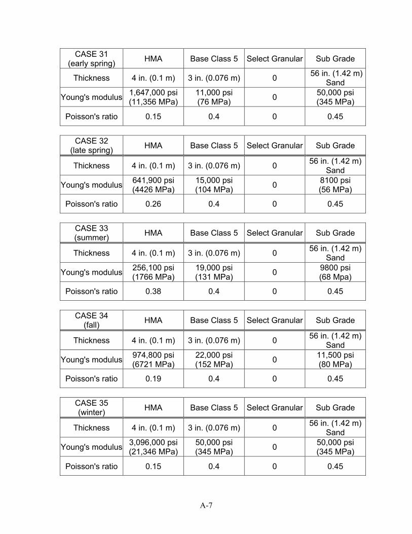
CASE 31 (early spring) HMA Base Class 5 Select Granular Sub Grade
Thickness 4 in. (0.1 m) 3 in. (0.076 m) 0 56 in. (1.42 m) Sand
Young's modulus 1,647,000 psi (11,356 MPa)
11,000 psi (76 MPa) 0 50,000 psi
(345 MPa)
Poisson's ratio 0.15 0.4 0 0.45
CASE 32
(late spring) HMA Base Class 5 Select Granular Sub Grade
Thickness 4 in. (0.1 m) 3 in. (0.076 m) 0 56 in. (1.42 m) Sand
Young's modulus 641,900 psi (4426 MPa)
15,000 psi (104 MPa) 0 8100 psi
(56 MPa)
Poisson's ratio 0.26 0.4 0 0.45
CASE 33 (summer) HMA Base Class 5 Select Granular Sub Grade
Thickness 4 in. (0.1 m) 3 in. (0.076 m) 0 56 in. (1.42 m) Sand
Young's modulus 256,100 psi (1766 MPa)
19,000 psi (131 MPa) 0 9800 psi
(68 Mpa)
Poisson's ratio 0.38 0.4 0 0.45
CASE 34
(fall) HMA Base Class 5 Select Granular Sub Grade
Thickness 4 in. (0.1 m) 3 in. (0.076 m) 0 56 in. (1.42 m) Sand
Young's modulus 974,800 psi (6721 MPa)
22,000 psi (152 MPa) 0 11,500 psi
(80 MPa)
Poisson's ratio 0.19 0.4 0 0.45
CASE 35 (winter) HMA Base Class 5 Select Granular Sub Grade
Thickness 4 in. (0.1 m) 3 in. (0.076 m) 0 56 in. (1.42 m) Sand
Young's modulus 3,096,000 psi (21,346 MPa)
50,000 psi (345 MPa) 0 50,000 psi
(345 MPa)
Poisson's ratio 0.15 0.4 0 0.45
A-7

CASE 36 (early spring) HMA Base Class 5 Select Granular Sub Grade
Thickness 8 in. (0.2 m) 3 in. (0.076 m) 0 52 in. (1.32 m) Sand
Young's modulus 1,647,000 psi (11,356 MPa)
11,000 psi (76 MPa) 0 50,000 psi
(345 MPa)
Poisson's ratio 0.15 0.4 0 0.45
CASE 37
(late spring) HMA Base Class 5 Select Granular Sub Grade
Thickness 8 in. (0.2 m) 3 in. (0.076 m) 0 52 in. (1.32 m) Sand
Young's modulus 641,900 psi (4426 MPa)
15,000 psi (104 MPa) 0 8100 psi
(56 MPa)
Poisson's ratio 0.26 0.4 0 0.45
CASE 38 (summer) HMA Base Class 5 Select Granular Sub Grade
Thickness 8 in. (0.2 m) 3 in. (0.076 m) 0 52 in. (1.32 m) Sand
Young's modulus 256,100 psi (1766 MPa)
19,000 psi (131 MPa) 0 9800 psi
(68 Mpa)
Poisson's ratio 0.38 0.4 0 0.45
CASE 39
(fall) HMA Base Class 5 Select Granular Sub Grade
Thickness 8 in. (0.2 m) 3 in. (0.076 m) 0 52 in. (1.32 m) Sand
Young's modulus 974,800 psi (6721 MPa)
22,000 psi (152 MPa) 0 11,500 psi
(80 MPa)
Poisson's ratio 0.19 0.4 0 0.45
CASE 40 (winter) HMA Base Class 5 Select Granular Sub Grade
Thickness 8 in. (0.2 m) 3 in. (0.076 m) 0 52 in. (1.32 m) Sand
Young's modulus 3,096,000 psi (21,346 MPa)
50,000 psi (345 MPa) 0 50,000 psi
(345 MPa)
Poisson's ratio 0.15 0.4 0 0.45
A-8

CASE 41 (early spring) HMA Base Class 5 Select Granular Sub Grade
Thickness 12 in. (0.3 m) 3 in. (0.076 m) 0 48 in. (1.22 m) Sand
Young's modulus 1,647,000 psi (11,356 MPa)
11,000 psi (76 MPa) 0 50,000 psi
(345 MPa)
Poisson's ratio 0.15 0.4 0 0.45
CASE 42
(late spring) HMA Base Class 5 Select Granular Sub Grade
Thickness 12 in. (0.3 m) 3 in. (0.076 m) 0 48 in. (1.22 m) Sand
Young's modulus 641,900 psi (4426 MPa)
15,000 psi (104 MPa) 0 8100 psi
(56 MPa)
Poisson's ratio 0.26 0.4 0 0.45
CASE 43 (summer) HMA Base Class 5 Select Granular Sub Grade
Thickness 12 in. (0.3 m) 3 in. (0.076 m) 0 48 in. (1.22 m) Sand
Young's modulus 256,100 psi (1766 MPa)
19,000 psi (131 MPa) 0 9800 psi
(68 Mpa)
Poisson's ratio 0.38 0.4 0 0.45
CASE 44
(fall) HMA Base Class 5 Select Granular Sub Grade
Thickness 12 in. (0.3 m) 3 in. (0.076 m) 0 48 in. (1.22 m) Sand
Young's modulus 974,800 psi (6721 MPa)
22,000 psi (152 MPa) 0 11,500 psi
(80 MPa)
Poisson's ratio 0.19 0.4 0 0.45
CASE 45 (winter) HMA Base Class 5 Select Granular Sub Grade
Thickness 12 in. (0.3 m) 3 in. (0.076 m) 0 48 in. (1.22 m) Sand
Young's modulus 3,096,000 psi (21,346 MPa)
50,000 psi (345 MPa) 0 50,000 psi
(345 MPa)
Poisson's ratio 0.15 0.4 0 0.45
A-9

CASE 46 (early spring) HMA Base Class 5 Select Granular Sub Grade
Thickness 4 in. (0.1 m) 12 in. (0.3 m) 0 47 in. (1.2 m) Clay loam
Young's modulus 1,647,000 psi (11,356 MPa)
11,000 psi (76 MPa) 0 50,000 psi
(345 MPa)
Poisson's ratio 0.15 0.4 0 0.45
CASE 47
(late spring) HMA Base Class 5 Select Granular Sub Grade
Thickness 4 in. (0.1 m) 12 in. (0.3 m) 0 47 in. (1.2 m) Clay loam
Young's modulus 641,900 psi (4426 MPa)
15,000 psi (104 MPa) 0 5100 psi
(35 MPa)
Poisson's ratio 0.26 0.4 0 0.45
CASE 48 (summer) HMA Base Class 5 Select Granular Sub Grade
Thickness 4 in. (0.1 m) 12 in. (0.3 m) 0 47 in. (1.2 m) Clay loam
Young's modulus 256,100 psi (1766 MPa)
19,000 psi (131 MPa) 0 6200 psi
(43 MPa)
Poisson's ratio 0.38 0.4 0 0.45
CASE 49
(fall) HMA Base Class 5 Select Granular Sub Grade
Thickness 4 in. (0.1 m) 12 in. (0.3 m) 0 47 in. (1.2 m) Clay loam
Young's modulus 974,800 psi (6721 MPa)
22,000 psi (152 MPa) 0 7300 psi
(51 MPa)
Poisson's ratio 0.19 0.4 0 0.45
CASE 50 (winter) HMA Base Class 5 Select Granular Sub Grade
Thickness 4 in. (0.1 m) 12 in. (0.3 m) 0 47 in. (1.2 m) Clay loam
Young's modulus 3,096,000 psi (21,346 MPa)
50,000 psi (345 MPa) 0 50,000 psi
(345 MPa)
Poisson's ratio 0.15 0.4 0 0.45
A-10
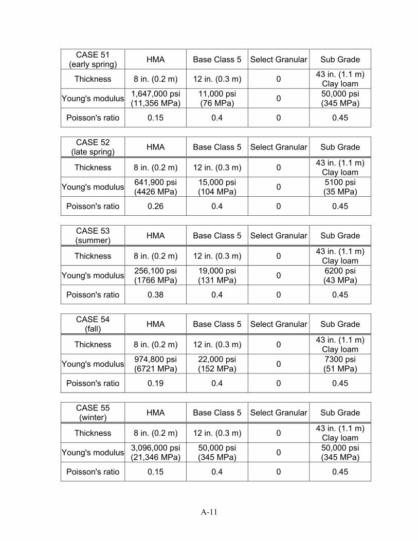
CASE 51 (early spring) HMA Base Class 5 Select Granular Sub Grade
Thickness 8 in. (0.2 m) 12 in. (0.3 m) 0 43 in. (1.1 m) Clay loam
Young's modulus 1,647,000 psi (11,356 MPa)
11,000 psi (76 MPa) 0 50,000 psi
(345 MPa)
Poisson's ratio 0.15 0.4 0 0.45
CASE 52
(late spring) HMA Base Class 5 Select Granular Sub Grade
Thickness 8 in. (0.2 m) 12 in. (0.3 m) 0 43 in. (1.1 m) Clay loam
Young's modulus 641,900 psi (4426 MPa)
15,000 psi (104 MPa) 0 5100 psi
(35 MPa)
Poisson's ratio 0.26 0.4 0 0.45
CASE 53 (summer) HMA Base Class 5 Select Granular Sub Grade
Thickness 8 in. (0.2 m) 12 in. (0.3 m) 0 43 in. (1.1 m) Clay loam
Young's modulus 256,100 psi (1766 MPa)
19,000 psi (131 MPa) 0 6200 psi
(43 MPa)
Poisson's ratio 0.38 0.4 0 0.45
CASE 54
(fall) HMA Base Class 5 Select Granular Sub Grade
Thickness 8 in. (0.2 m) 12 in. (0.3 m) 0 43 in. (1.1 m) Clay loam
Young's modulus 974,800 psi (6721 MPa)
22,000 psi (152 MPa) 0 7300 psi
(51 MPa)
Poisson's ratio 0.19 0.4 0 0.45
CASE 55 (winter) HMA Base Class 5 Select Granular Sub Grade
Thickness 8 in. (0.2 m) 12 in. (0.3 m) 0 43 in. (1.1 m) Clay loam
Young's modulus 3,096,000 psi (21,346 MPa)
50,000 psi (345 MPa) 0 50,000 psi
(345 MPa)
Poisson's ratio 0.15 0.4 0 0.45
A-11

Appendix B
ABAQUS

Appendix B – ABAQUS ABAQUS Task Description
The following is a step-by-step procedure required for completing (i.e. creating a model in ABAQUS/CAE to processing the output) one case study. This procedure has three main steps: creating an ABAQUS/CAE database, exporting data, and interpreting data. Within these steps are numerous sub-steps. 1. Create an ABAQUS/CAE database
a) Drafting the pavement system. This is done by entering the Part Module to name and assign a model type (i.e. two-dimensional or three-dimensional). Then the sketch module is entered to draw the prism representing the pavement system. To account for the varying layer thicknesses of all the layers (i.e. AC, base/subbase, and subgrade), the pavement structure model was partitioned into 0.025 m (1 in.) and 0.05 m (2 in.) elemental layers. By partitioning the model into small increments, only one pavement structure model had to be created in ABAQUS/CAE instead of eleven different models differing in layer thicknesses. This is accomplished using a sketching program (similar to AutoCAD 2000) in ABAQUS/CAE. A three-dimensional model is more time consuming to draft in comparison to a two-dimensional model.
b) Assigning material sections and properties to the model. This is done by entering the Property Module. In this module the material information is entered into a material dialog box followed by a section dialog box where material information is assigned to named sections. Finally, the section definitions, which contain material information, are assigned to the model.
c) If the model has different parts (e.g. the pavement and tire or different layers) that are drawn separately, the Assembly Module is needed. If the entire pavement system is drawn as one and then partitioned into sections, the Assembly Module is not needed. If there are separate parts they are moved and rotated so that they are in position in the Assembly Module. d) Creating time steps for loading in the Step Module. ABAQUS/CAE requires that a time step is created even if the model has static loading. The initial step in ABAQUS/CAE is a stress-free step. The user creates step 1 which follows the initial step and this is when the static load is applied to the model. If dynamic loading is required, numerous time steps would be created and load would be applied or removed at each of these time steps.
e) ABAQUS/CAE has the option of defining a contact (e.g. friction or smooth) interface. If the entire pavement system is drawn as one and then partitioned, ABAQUS/CAE treats the layer of the pavement system like they are glued together so there is no need for the Interaction Module. If there are separate parts of the pavement system, interaction properties (i.e. friction, contact) between the parts of the model are created and assigned in the Interaction Module. f) Creating and assigning the loading conditions and boundary conditions to the assembled pavement-tire system.
g) Creating a mesh for the pavement-tire system in the Mesh Module. This is done by seeding the edges of the model. The edges can be seeded by number of elements,
B-1

size of elements, or by a biased number (i.e. the number of seeds increases or decreases along the length of the edge). Once the edges are seeded, ABAQUS/CAE connects the edge seeds with lines to form the mesh. h) Submitting the job to ABAQUS/CAE. This is done in the in the Job Module. Once submitted, the ABAQUS/CAE database is processed. i) Upon completion, output files are created by ABAQUS/CAE or by the user for data exportation. This is done by selecting the information (i.e. stresses, strains, etc.) that is needed in the Visualization Module. For each case considered, an input file is generated with the extension *.inp (e.g. case1.inp). The *.inp file is run to create an initial output file with the extension *.odb (e.g. case1.odb). Once this is completed the stress distributions (σxx, σyy along the top and bottom of the HMA layer as well as σxx along the edge of the transverse crack and through the center of loading) are extracted from ABAQUS/CAE. ABAQUS/CAE labels the axis with numbers (1, 2, 3) instead of letters (x, y, z). Therefore the output (e.g. stresses) is labeled S11, S22, and S33. In this thesis the stress results are presented using the notation of sigma (σ) and x, y, and z to denote the direction. The labels S11, S22, and S33 must be changed manually to reflect the σxx, σyy, and σzz notation. Using the stress linearization command in ABAQUS/CAE, the value of the stress at the nodal points of the model are extracted from the *.odb file. When using the stress linearization command, ABAQUS/CAE selects a local coordinate system. The line which is defined to obtain the stresses of interest becomes the “1” or “x” axis even if it is globally labeled the “2” axis for example. The direction perpendicular and in the same horizontal plane to the defined line becomes the “3” or “y” axis. ABAQUS/CAE does not specifically state that it defines a local coordinate system in the program. Once the data files are created, they are then transferred from ABAQUS/CAE on the super computer to the desk top computer as a text file with the extension *.rpt. The text files are then opened in Microsoft Excel. Once in Excel, the data is manipulated so that no irrelevant data is included and the sign convention is changed so that compression is positive and tension is negative. Once these spreadsheets are completed, a master case spreadsheet is made. This spreadsheet includes the six stress distributions for a cracked model and six stress distributions for an uncracked model for one specific case. Creating the stress distributions is only part of the reported output.
j) Element numbers are recorded (by hand) of the desired elements for use later on while in the Visualization Module. The vertical stresses in the base below the edge of the transverse crack and below the center of loading are of interest. To obtain these stresses, the output file (*.odb file) from ABAQUS/CAE is opened and using the probe value command the two elements located below the edge of the transverse crack and below the center of loading are selected by pointing and clicking on them. The specified value is then reported. This is recorded and later entered into a chart.
B-2

FIGURE C.1: Summary cross section for case 1, C – stress in cracked pavement, NC – stress in pavement with no crack, CNR – crack/no crack (stress) ratio)
C-2

FIGURE C.2: Summary cross section for case 2, (C – stress in cracked pavement, NC – stress in pavement with no crack, CNR – crack/no crack (stress) ratio)
C-3

FIGURE C.3: Summary cross section for case 3, (C – stress in cracked pavement, NC – stress in pavement with no crack, CNR – crack/no crack (stress) ratio)
C-4
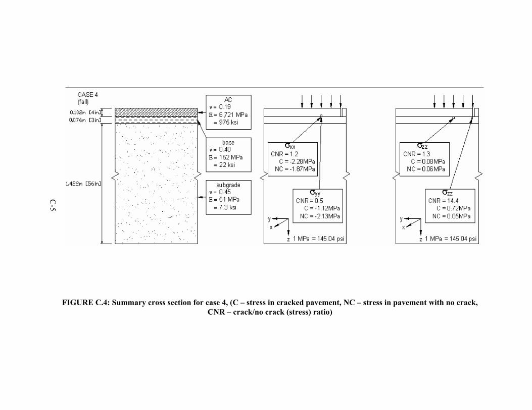
FIGURE C.4: Summary cross section for case 4, (C – stress in cracked pavement, NC – stress in pavement with no crack, CNR – crack/no crack (stress) ratio)
C-5

FIGURE C.5: Summary cross section for case 5, (C – stress in cracked pavement, NC – stress in pavement with no crack, CNR – crack/no crack (stress) ratio)
C-6

FIGURE C.6: Summary cross section for case 6, (C – stress in cracked pavement, NC – stress in pavement with no crack, CNR – crack/no crack (stress) ratio)
C-7

FIGURE C.7: Summary cross section for case 7, (C – stress in cracked pavement, NC – stress in pavement with no crack, CNR – crack/no crack (stress) ratio)
C-8

FIGURE C.8: Summary cross section for case 8, (C – stress in cracked pavement, NC – stress in pavement with no crack, CNR – crack/no crack (stress) ratio)
C-9

FIGURE C.9: Summary cross section for case 9, (C – stress in cracked pavement, NC – stress in pavement with no crack, CNR – crack/no crack (stress) ratio)
C-10

FIGURE C.10: Summary cross section for case 10, (C – stress in cracked pavement, NC – stress in pavement with no crack, CNR – crack/no crack (stress) ratio)
C-11

FIGURE C.11: Summary cross section for case 11, (C – stress in cracked pavement, NC – stress in pavement with no crack, CNR – crack/no crack (stress) ratio)
C-12

FIGURE C.12: Summary cross section for case 12, (C – stress in cracked pavement, NC – stress in pavement with no crack, CNR – crack/no crack (stress) ratio)
C-13

FIGURE C.13: Summary cross section for case 13, (C – stress in cracked pavement, NC – stress in pavement with no crack, CNR – crack/no crack (stress) ratio)
C-14

FIGURE C.14: Summary cross section for case 14, (C – stress in cracked pavement, NC – stress in pavement with no crack, CNR – crack/no crack (stress) ratio)
C-15
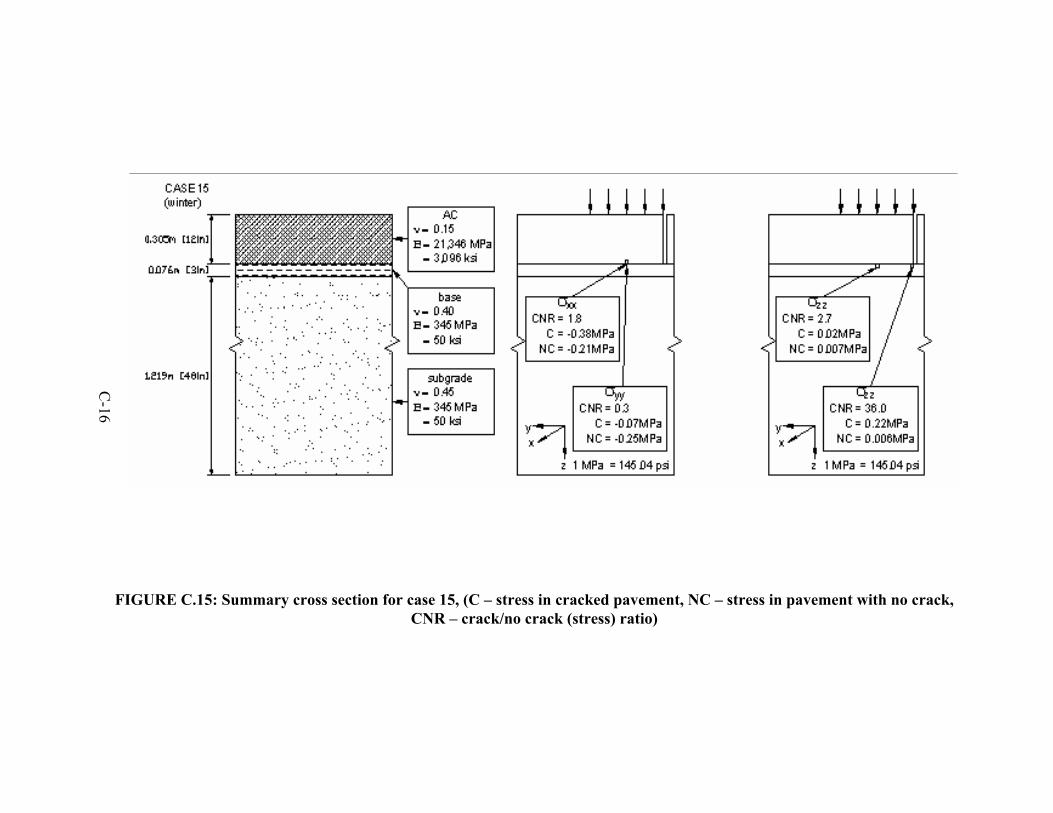
FIGURE C.15: Summary cross section for case 15, (C – stress in cracked pavement, NC – stress in pavement with no crack, CNR – crack/no crack (stress) ratio)
C-16

FIGURE C.16: Summary cross section for case 16, (C – stress in cracked pavement, NC – stress in pavement with no crack, CNR – crack/no crack (stress) ratio)
C-17

FIGURE C.17: Summary cross section for case 17, (C – stress in cracked pavement, NC – stress in pavement with no crack, CNR – crack/no crack (stress) ratio)
C-18

FIGURE C.18: Summary cross section for case 18, (C – stress in cracked pavement, NC – stress in pavement with no crack, CNR – crack/no crack (stress) ratio)
C-19
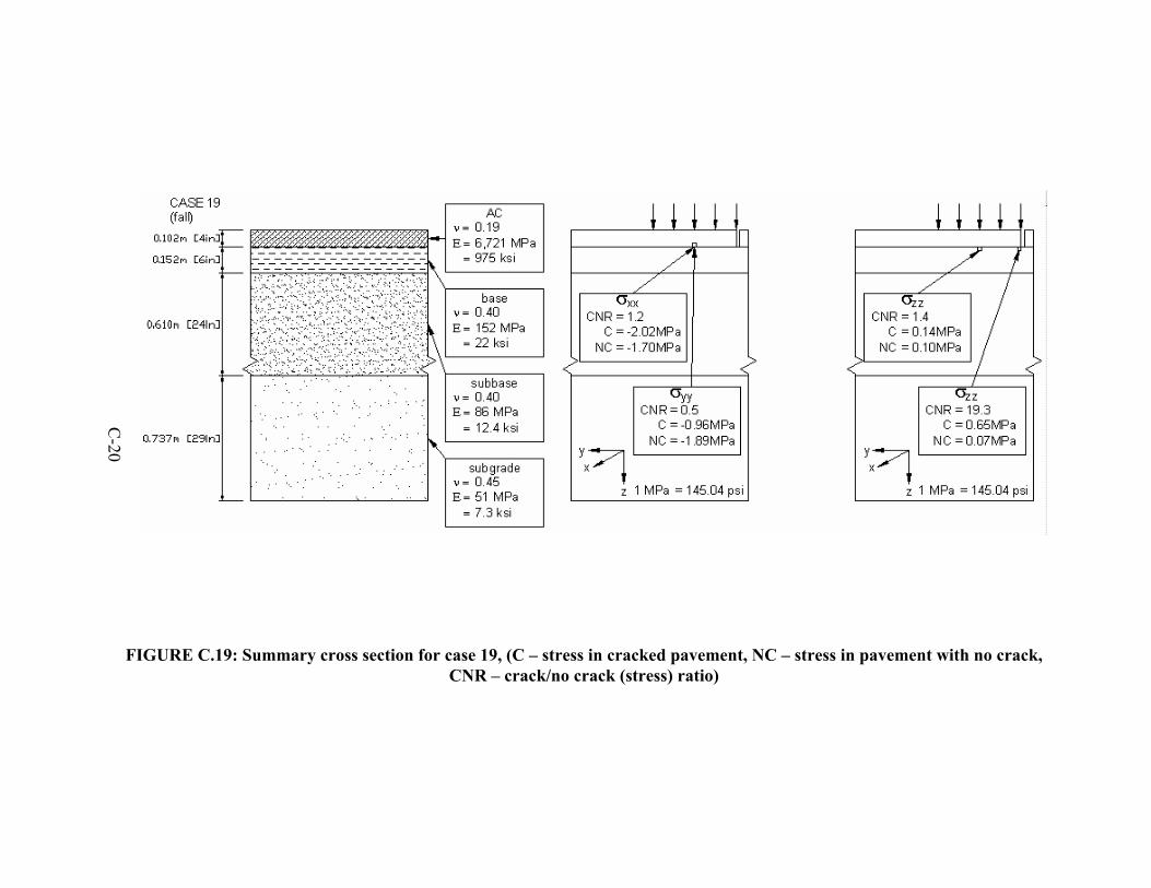
FIGURE C.19: Summary cross section for case 19, (C – stress in cracked pavement, NC – stress in pavement with no crack, CNR – crack/no crack (stress) ratio)
C-20

FIGURE C.20: Summary cross section for case 20, (C – stress in cracked pavement, NC – stress in pavement with no crack, CNR – crack/no crack (stress) ratio)
C-21
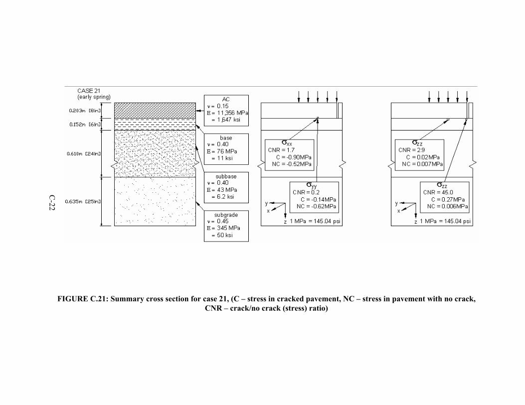
FIGURE C.21: Summary cross section for case 21, (C – stress in cracked pavement, NC – stress in pavement with no crack, CNR – crack/no crack (stress) ratio)
C-22

FIGURE C.22: Summary cross section for case 22, (C – stress in cracked pavement, NC – stress in pavement with no crack, CNR – crack/no crack (stress) ratio)
C-23

FIGURE C.23: Summary cross section for case 23, (C – stress in cracked pavement, NC – stress in pavement with no crack, CNR – crack/no crack (stress) ratio)
C-24

FIGURE C.24: Summary cross section for case 24, (C – stress in cracked pavement, NC – stress in pavement with no crack, CNR – crack/no crack (stress) ratio)
C-25

FIGURE C.25: Summary cross section for case 25, (C – stress in cracked pavement, NC – stress in pavement with no crack, CNR – crack/no crack (stress) ratio)
C-26

FIGURE C.26: Summary cross section for case 26, (C – stress in cracked pavement, NC – stress in pavement with no crack, CNR – crack/no crack (stress) ratio)
C-27
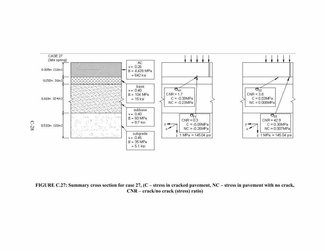
FIGURE C.27: Summary cross section for case 27, (C – stress in cracked pavement, NC – stress in pavement with no crack, CNR – crack/no crack (stress) ratio)
C-28

FIGURE C.28: Summary cross section for case 28, (C – stress in cracked pavement, NC – stress in pavement with no crack, CNR – crack/no crack (stress) ratio)
C-29

FIGURE C.29: Summary cross section for case 29, (C – stress in cracked pavement, NC – stress in pavement with no crack, CNR – crack/no crack (stress) ratio)
C-30
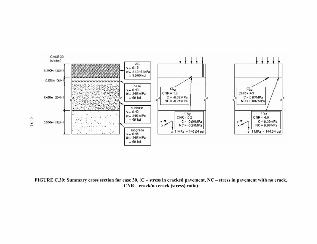
FIGURE C.30: Summary cross section for case 30, (C – stress in cracked pavement, NC – stress in pavement with no crack, CNR – crack/no crack (stress) ratio)
C-31

FIGURE C.31: Summary cross section for case 31, (C – stress in cracked pavement, NC – stress in pavement with no crack, CNR – crack/no crack (stress) ratio)
C-32
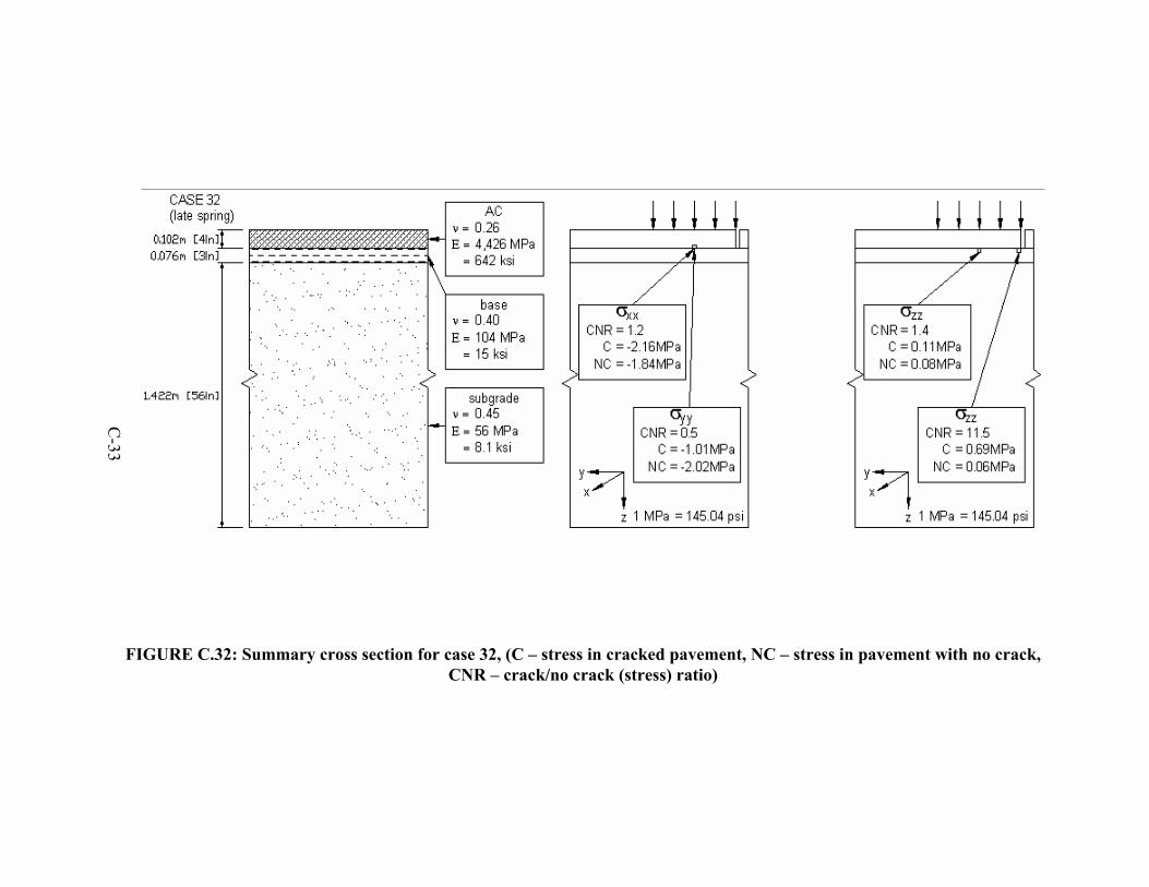
FIGURE C.32: Summary cross section for case 32, (C – stress in cracked pavement, NC – stress in pavement with no crack, CNR – crack/no crack (stress) ratio)
C-33

FIGURE C.33: Summary cross section for case 33, (C – stress in cracked pavement, NC – stress in pavement with no crack, CNR – crack/no crack (stress) ratio)
C-34

FIGURE C.34: Summary cross section for case 34, (C – stress in cracked pavement, NC – stress in pavement with no crack, CNR – crack/no crack (stress) ratio)
C-35

FIGURE C.35: Summary cross section for case 35, (C – stress in cracked pavement, NC – stress in pavement with no crack, CNR – crack/no crack (stress) ratio)
C-36

FIGURE C.36: Summary cross section for case 36, (C – stress in cracked pavement, NC – stress in pavement with no crack, CNR – crack/no crack (stress) ratio)
C-37

FIGURE C.37: Summary cross section for case 37, (C – stress in cracked pavement, NC – stress in pavement with no crack, CNR – crack/no crack (stress) ratio)
C-38

FIGURE C.38: Summary cross section for case 38, (C – stress in cracked pavement, NC – stress in pavement with no crack, CNR – crack/no crack (stress) ratio)
C-39
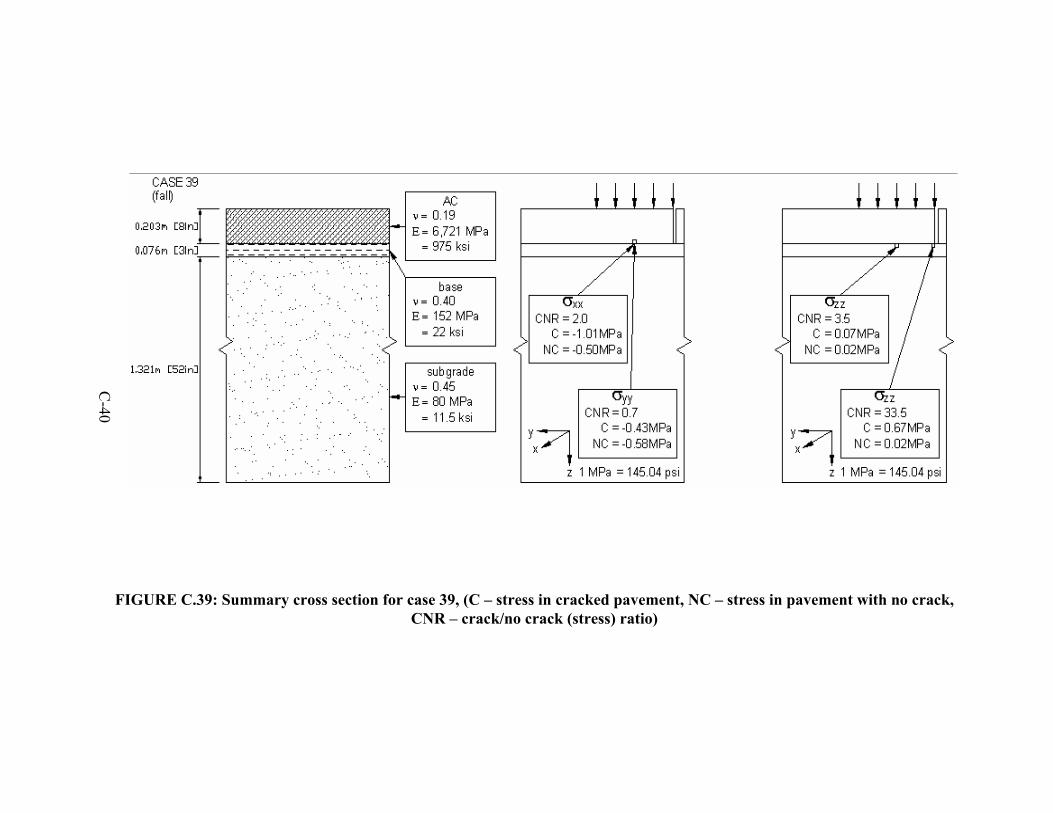
FIGURE C.39: Summary cross section for case 39, (C – stress in cracked pavement, NC – stress in pavement with no crack, CNR – crack/no crack (stress) ratio)
C-40
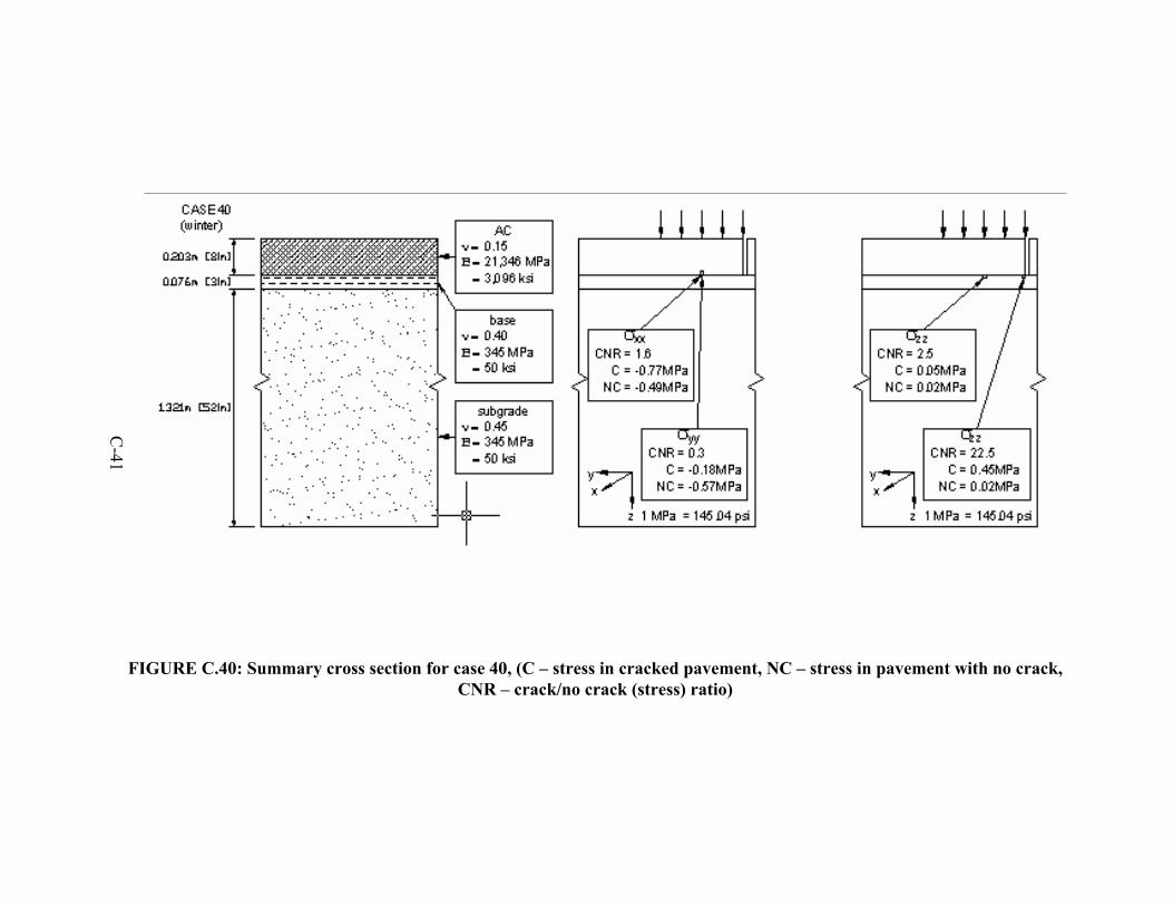
FIGURE C.40: Summary cross section for case 40, (C – stress in cracked pavement, NC – stress in pavement with no crack, CNR – crack/no crack (stress) ratio)
C-41

FIGURE C.41: Summary cross section for case 41, (C – stress in cracked pavement, NC – stress in pavement with no crack, CNR – crack/no crack (stress) ratio)
C-42

FIGURE C.42: Summary cross section for case 42, (C – stress in cracked pavement, NC – stress in pavement with no crack, CNR – crack/no crack (stress) ratio)
C-43

FIGURE C.43: Summary cross section for case 43, (C – stress in cracked pavement, NC – stress in pavement with no crack, CNR – crack/no crack (stress) ratio)
C-44

FIGURE C.44: Summary cross section for case 44, (C – stress in cracked pavement, NC – stress in pavement with no crack, CNR – crack/no crack (stress) ratio)
C-45

FIGURE C.45: Summary cross section for case 45, (C – stress in cracked pavement, NC – stress in pavement with no crack, CNR – crack/no crack (stress) ratio)
C-46

FIGURE C.46: Summary cross section for case 46, (C – stress in cracked pavement, NC – stress in pavement with no crack, CNR – crack/no crack (stress) ratio)
C-47

FIGURE C.47: Summary cross section for case 47, (C – stress in cracked pavement, NC – stress in pavement with no crack, CNR – crack/no crack (stress) ratio)
C-48

FIGURE C.48: Summary cross section for case 48, (C – stress in cracked pavement, NC – stress in pavement with no crack, CNR – crack/no crack (stress) ratio)
C-49

FIGURE C.49: Summary cross section for case 49, (C – stress in cracked pavement, NC – stress in pavement with no crack, CNR – crack/no crack (stress) ratio)
C-50
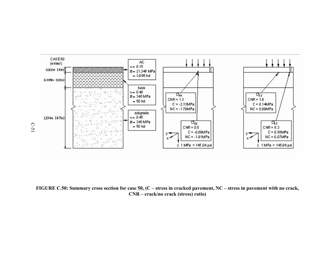
FIGURE C.50: Summary cross section for case 50, (C – stress in cracked pavement, NC – stress in pavement with no crack, CNR – crack/no crack (stress) ratio)
C-51
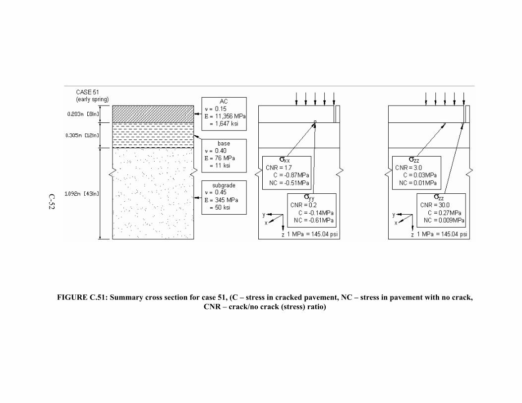
FIGURE C.51: Summary cross section for case 51, (C – stress in cracked pavement, NC – stress in pavement with no crack, CNR – crack/no crack (stress) ratio)
C-52

FIGURE C.52: Summary cross section for case 52, (C – stress in cracked pavement, NC – stress in pavement with no crack, CNR – crack/no crack (stress) ratio)
C-53

FIGURE C.53: Summary cross section for case 53, (C – stress in cracked pavement, NC – stress in pavement with no crack, CNR – crack/no crack (stress) ratio)
C-54

FIGURE C.54: Summary cross section for case 54, (C – stress in cracked pavement, NC – stress in pavement with no crack, CNR – crack/no crack (stress) ratio)
C-55

FIGURE C.55: Summary cross section for case 55, (C – stress in cracked pavement, NC – stress in pavement with no crack, CNR – crack/no crack (stress) ratio)
C-56