INVESTIGATION OF AN ENERGY EFFICIENT PUMP SPEED …

INVESTIGATION OF AN ENERGY EFFICIENT PUMP SPEED CONTROL

ALGORITHM FOR CONTROLLING SUMP LEVEL

by

Josh Dubey

A thesis submitted to the Faculty of the University of Delaware in partial

fulfillment of the requirements for the Master of Science in Electrical and Computer

Engineering

Fall 2018

© 2018 Josh Dubey

All Rights Reserved

INVESTIGATION OF AN ENERGY EFFICIENT PUMP SPEED CONTROL

ALGORITHM FOR CONTROLLING SUMP LEVEL

by

Josh Dubey

Approved: __________________________________________________________

Keith Goossen, Ph.D.

Professor in charge of thesis on behalf of the Advisory Committee

Approved: __________________________________________________________

Kenneth E. Barner, Ph.D.

Chair of the Department of Electrical and Computer Engineering

Approved: __________________________________________________________

Levi T. Thompson, Ph.D.

Dean of the College of Engineering

Approved: __________________________________________________________

Douglas J. Doren, Ph.D.

Interim Vice Provost for the Office of Graduate and Professional

Education

iii

ACKNOWLEDGMENTS

I wish to thank my parents, friends and my advisor for the continued support

necessary to complete my thesis.

iv

TABLE OF CONTENTS

LIST OF TABLES ......................................................................................................... v

LIST OF FIGURES ....................................................................................................... vi ABSTRACT ................................................................................................................ viii

Chapter

1 INTRODUCTION .............................................................................................. 1

2 THEORY ............................................................................................................ 4

2.1 Background on Pumping ........................................................................... 4

2.2 Variable Level Control .............................................................................. 7

3 EXPERIMENTAL SETUP ................................................................................ 9

3.1 Description of Pilot Scale Design .............................................................. 9

3.1.1 Control Hardware and Software .................................................... 9 3.1.2 Human Machine Interface ........................................................... 15

3.1.3 System Characteristics ................................................................. 16

3.2 Proposed Algorithm ................................................................................. 19 3.3 Test Flow Regime .................................................................................... 22

4 RESULTS AND DISCUSSION ....................................................................... 23

5 CONCLUSION ................................................................................................ 29

REFERENCES ............................................................................................................. 30

Appendix

MATLAB CODE ............................................................................................. 31

v

LIST OF TABLES

Table 4.1 Experimental SE values and % Savings. ................................................... 24

Table 4.2 Experimental Process Parameter Variables ............................................... 28

vi

LIST OF FIGURES

Figure 2.1 An arbitrary pump system with three system curves, S1, S2 and S3.

Isoefficiency lines are plotted as well. Adapted from 'Variable speed

wastewater pumping', 2013, White Paper, 7. ............................................ 5

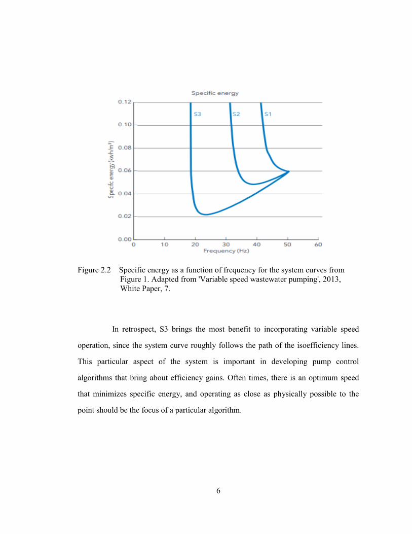
Figure 2.2 Specific energy as a function of frequency for the system curves from

Figure 1. Adapted from 'Variable speed wastewater pumping', 2013,

White Paper, 7. .......................................................................................... 6

Figure 2.3 Pump speed as a function of sump level for linear and concave up

control relationships. ................................................................................. 8

Figure 3.1 Control hardware for the pump station shown. From left to right, the

Micrologix PLC, the VFD, and the two power supplies for field

devices. .................................................................................................... 11

Figure 3.2 The main program file of the pump station control logic in RSLogix

Micro Starter. ........................................................................................... 12

Figure 3.3 A section of the ladder logic for the nonlinear control algorithm. The

exact algorithm is programmed in the block called PUMP SPEED

ALGORITHM OUTPUT. ....................................................................... 13

Figure 3.4 A section of the ladder logic for PID control of the pump. This logic

is executed mostly to return the sump level to a certain value

following an experimental test run. ......................................................... 14

Figure 3.5 The HMI for the pump station. A visualization of the process with real

time values is shown on the left, while a historical data trend of

process variables is shown graphically on the right ................................ 15

Figure 3.6 (a) Simulated variable speed pump curves for the experiment, with the

system curve developed for Level=50.8 cm (20 in.) and (b) Pump

efficiencies at variable speeds ................................................................. 17

Figure 3.7 The pilot scale pump station ..................................................................... 18

Figure 3.8 Experimental concave up speed control curves. “A” is the curvature

value. The sump tank level is shown here in centimeters ....................... 19

vii

Figure 3.9 Sump inlet flow rate (liters/min) as a function of time for one

experimental cycle. This exact flow regime is repeated for all cycles. ... 22

Figure 4.1 (a) Specific Energy and (b) Specific Energy Savings plotted for

experimental data. The markers are averages of each of the three test

cycles for each value of curvature. A second order fit of the savings

points is also plotted to show the experimental correlation .................... 23

Figure 4.2 (a) Average Level, (b) Speed and (c) Maximum Speed collected from

data for each curvature value. Each marker represents the average of

three test cycles for the corresponding curvature value. ......................... 25

Figure 4.3 (a) Pump Speed, (b) Sump Level and (c) Inlet Flow Rate collected

over the cycle time of 1800 seconds for each curvature value. Each

line represents the average of three test cycles at that particular

instance. ................................................................................................... 26

Figure 4.4 Active Power plotted for linear and curvature values of 7.5 and 15 ...... 27

viii

ABSTRACT

This thesis explores a new nonlinear control algorithm for variable speed

centrifugal pumps at water/wastewater pump stations that leads to specific energy

savings over the conventional linear one. The algorithm is useful for facilities where

pump speed is a linear function of liquid level in order to transport fluid and smooth

inflow peaks. A nonlinearity in the form of a quadratic term is added to the

conventional linear one in order to produce efficiency gains, with a single parameter,

curvature, varied to optimize energy savings. Results obtained by implementing the

new algorithm on a pilot-scale pump station show significant energy savings for fixed

pump flow, with a parabolic correlation of specific energy savings versus curvature of

the nonlinear quadratic determined. In addition, the cost of implementing this

algorithm is minimal to none, so the work presented has significant industrial

potential.

1

Chapter 1

INTRODUCTION

Growing awareness of issues such as sustainable energy use and energy

efficiency have prompted interest in energy saving research in various industrial

applications, including pumping systems. Particularly, Goldstein and Smith

[1] reported that nearly 4% of United States electricity is consumed by wastewater

treatment plants and almost 80% of the electricity in the wastewater treatment process

is used by pumps. Based on the large proportion of energy used for pumping, and the

vast number of wastewater plants across the country, just a small reduction in energy

use can lead to large savings. Here, we report a new control algorithm for sump

pumping systems, for example in wastewater treatment plants that results in up to 4 %

savings compared to the currently used control algorithms.

In general, savings in pump energy can be achieved in two main ways. One is

by designing more efficient pumps. Another, discussed and presented here, is

improving pump performance with effective control strategies. The latter often times

involves employing speed control of centrifugal pumps with frequency regulated by

Variable Speed Drives (VFD). By regulating pump speed according to process

parameters such as tank level, pump power can be reduced significantly compared to

constant-speed control. However, the precise speed control algorithm can result in

additional savings. Roughly, there are two algorithmic approaches. One is to attempt

to maintain speed at the best-efficiency point of the pump. Bakman, Geverkov and

Vodovozov [2] discussed a method for single and multi-pump predictive control to

2

maintain operation in the best-efficiency region. Tang and Zhang [3] considered a

model predictive control approach to improve operational efficiency incorporating

variables such as TOU tariff and water demand. Zhang, Zhen and Kusiak [4]

developed a scheduling model to generate energy optimal operational schedules for

wastewater pump systems. As discussed in [2-4], most of the pump control research

has focused on predictive control strategies, with emphasis on scheduling variable

speed centrifugal pump runs based on modelling of future inlet flow rates. While these

methods have potential to bring about efficiency gains and better operation, they are

often costly and require large investments in existing pump control systems.

Therefore, a simpler more cost-effective control strategy that results in energy savings

is highly desirable.

Wastewater treatment plants as well as other applications usually have an input

sump for collecting inlet flows. Since the inlet flows are highly variable, it is essential

to have an effective control strategy that will adjust outflow. For sump stations that

employ centrifugal outflow pumps on variable speed drives, two types of control

strategies exist. Constant sump level control, a form of closed loop Proportional-

Integral (PI) control where pump frequency is adjusted to maintain the tank level at a

desired set point, is one method. Variable level control, a soft control strategy where

pump frequency is a linear proportional function of sump level, is the second method,

and has the advantage of smoothing large inflow peaks compared to constant level

control. In the latter strategy, pump speed increases as inlet flow increases and level

rises, with no actual level set point and error variable, until a new equilibrium level is

achieved. All reported algorithms for speed-level control show pump speed increasing

linearly with level. In this paper, a nonlinear, quadratic term is added to the speed

3

versus level function and is explored experimentally to show lower energy use

compared to the linear-only function. Particularly, using a quadratic negative-

curvature function, a 4 % reduction in energy is found for a particular curvature.

While the exact curvature for a particular sump pumping system that minimizes

energy may depend upon the particular pumping system, we demonstrate here that

adding the quadratic into the algorithm can result in significant energy savings, and

potentially reduce overall United States electricity consumption on the order of a tenth

of a percent.

4

Chapter 2

THEORY

2.1 Background on Pumping

Over the last 10-15 years, there has been a large increase in the number of

municipalities adapting variable frequency drives (VFDs) to their pump stations.

Advantages of variable speed operation include the potential of decreased energy use,

more flexibility and the ability to soft start pump motors to extend lifetime. While not

all pump stations are necessarily fit for variable speed operation, particularly those

who are solely lift stations with high static head, many accrue considerable benefit

from installing adopting these drives. Energy savings for centrifugal pumps on

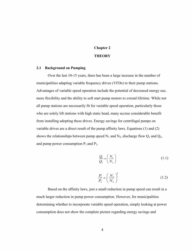
variable drives are a direct result of the pump affinity laws. Equations (1) and (2)

shows the relationships between pump speed N1 and N2, discharge flow Q1 and Q2,

and pump power consumption P1 and P2.

(1.1)

(1.2)

Based on the affinity laws, just a small reduction in pump speed can result in a

much larger reduction in pump power consumption. However, for municipalities

determining whether to incorporate variable speed operation, simply looking at power

consumption does not show the complete picture regarding energy savings and

1 1

2 2

Q N

Q N

3

1 1

2 2

P N

P N

5

potential payback. The most useful variable, and one that will be referred to in this

paper, is specific energy SE written as:

(1.3)

where E is the unit energy and V is the unit volume. Specific energy takes into

account the amount of discharge flow for a unit of energy consumed, and therefore

serves as the preferred statistic for comparing energy savings for different control

algorithms on a given pumping system. Figure 2.1 from Xylem Corporation [5] shows

an example of three different system curves operated by a single pump. Since the

static and dynamic head components are different for each system, the specific energy

curves shown in Figure 2.2 are dramatically different.

Figure 2.1 An arbitrary pump system with three system curves, S1, S2 and S3.

Isoefficiency lines are plotted as well. Adapted from 'Variable speed

wastewater pumping', 2013, White Paper, 7.

ESE

V

6

Figure 2.2 Specific energy as a function of frequency for the system curves from

Figure 1. Adapted from 'Variable speed wastewater pumping', 2013,

White Paper, 7.

In retrospect, S3 brings the most benefit to incorporating variable speed

operation, since the system curve roughly follows the path of the isoefficiency lines.

This particular aspect of the system is important in developing pump control

algorithms that bring about efficiency gains. Often times, there is an optimum speed

that minimizes specific energy, and operating as close as physically possible to the

point should be the focus of a particular algorithm.

7

2.2 Variable Level Control

For pump stations employing the technique known as variable level control,

pump speed is a function of sump level where the speed increases proportionally with

level. The pump speed will fluctuate with tank level until a temporary equilibrium

point is reached where the inlet flow matches the outlet flow from the sump. Thus far,

only algorithms where speed varies linearly with level have been in use, however

exploring adding a nonlinearity can potentially result in specific energy reductions for

pump systems. Especially for systems like S3 in Figure 2.2, it is possible that

developing an algorithm that results in a higher average sump level, and lower average

pump speed for a given operational period can bring about efficiency gains.

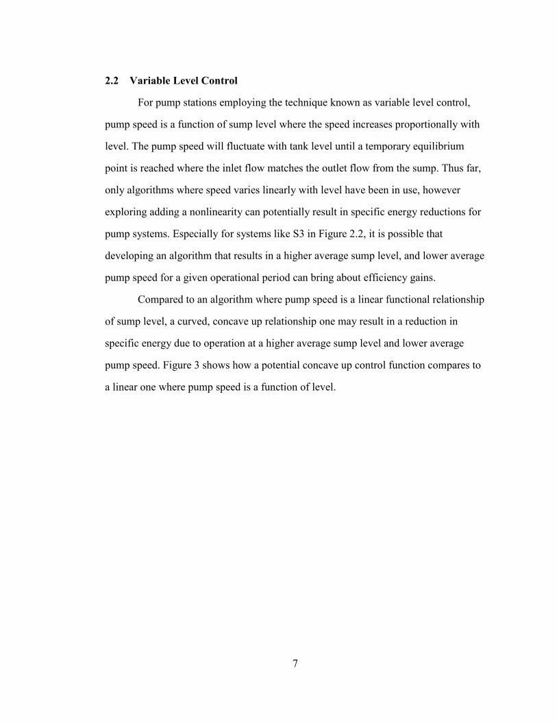
Compared to an algorithm where pump speed is a linear functional relationship

of sump level, a curved, concave up relationship one may result in a reduction in

specific energy due to operation at a higher average sump level and lower average

pump speed. Figure 3 shows how a potential concave up control function compares to

a linear one where pump speed is a function of level.

8

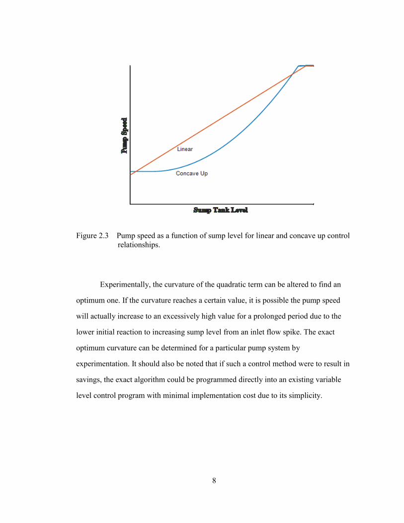
Figure 2.3 Pump speed as a function of sump level for linear and concave up control

relationships.

Experimentally, the curvature of the quadratic term can be altered to find an

optimum one. If the curvature reaches a certain value, it is possible the pump speed

will actually increase to an excessively high value for a prolonged period due to the

lower initial reaction to increasing sump level from an inlet flow spike. The exact

optimum curvature can be determined for a particular pump system by

experimentation. It should also be noted that if such a control method were to result in

savings, the exact algorithm could be programmed directly into an existing variable

level control program with minimal implementation cost due to its simplicity.

9

Chapter 3

EXPERIMENTAL SETUP

Testing of the proposed control algorithm was done experimentally on a pilot

scale pump station. Data was collected and analyzed to determine if there were

specific energy reductions. The exact methods used for developing the nonlinear

control algorithms are highlighted in this section.

3.1 Description of Pilot Scale Design

A pilot scale pump station is designed for experimenting with different

algorithms. A Xylem 0.75HP centrifugal pump is used to draw room temperature

water from a 58 centimeter (20 inch) sump tank that resides 0.61 meters (2 feet) below

the elevation of the pump. The pump frequency is controlled by a 1HP TECO-

Westinghouse Variable Speed Drive (VFD), which receives both run/stop and

frequency command via a 0-10V analog signal from an Allen Bradley Micrologix

Programmable Logic Controller (PLC). Water is pumped over a total distance of 10

feet from the sump to a 189 liter (50 gallon) tank that is located 9.5 feet above ground

level, which comprises the static head in the system.

3.1.1 Control Hardware and Software

The Micrologix PLC is used for controlling all operations of the pilot scale

pump station. The particular version used, the Micrologix 1400, has both analog and

digital inputs and outputs, enabling both continuous and discrete on-off control. This

particular series can receive 120 Volt AC digital signals, and has in excess of 16 dry

10

contact outputs that can send relay signals to field devices and motors, including the

run-stop command for the VFD. The power supplied to the controller is only sufficient

for powering the processer, so all field devices must be powered externally. For this

reason, a 24V DC external power supply is used for powering all analog and digital

transmitters and control valves. The VFD receives a digital input as a run/stop

command and a 0-10V analog signal for the motor frequency command. It also sends a

0-10V analog signal back to the PLC for a frequency feedback. The analog devices

used in the pump station include the VFD, a motorized control valve for modulating

flow to the sump tank, two flow sensors for measuring the input flow rate to the sump,

as well as a level transmitter, which records sump level and sends a voltage signal to

the PLC. Several digital devices are used, including two motorized ball valves, a

solenoid valve, and a momentary push button that is programmed to change the

operating mode of the station when pushed.

11

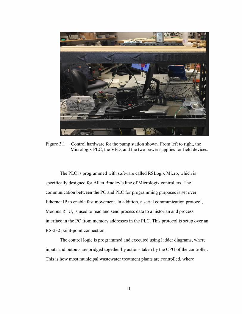
Figure 3.1 Control hardware for the pump station shown. From left to right, the

Micrologix PLC, the VFD, and the two power supplies for field devices.

The PLC is programmed with software called RSLogix Micro, which is

specifically designed for Allen Bradley’s line of Micrologix controllers. The

communication between the PC and PLC for programming purposes is set over

Ethernet IP to enable fast movement. In addition, a serial communication protocol,

Modbus RTU, is used to read and send process data to a historian and process

interface in the PC from memory addresses in the PLC. This protocol is setup over an

RS-232 point-point connection.

The control logic is programmed and executed using ladder diagrams, where

inputs and outputs are bridged together by actions taken by the CPU of the controller.

This is how most municipal wastewater treatment plants are controlled, where

12

multiple PLCs execute control logic across the entire process. In Figure 4, the main

page of the ladder program is shown:

Figure 3.2 The main program file of the pump station control logic in RSLogix

Micro Starter.

The ladder logic is executed from top to bottom at a particular scan rate set by

the user. The main routine (shown in Figure 3.2) is executed first, with subroutines

executed thereafter. For this setup, subroutines are created specifically for controlling

the pump speed based on sump level based on the experimental algorithms, for

controlling flow rate to the sump, and for controlling the pump via a typical

Proportional-Integral-Derivative (PID) control loop for experimental purposes. Figure

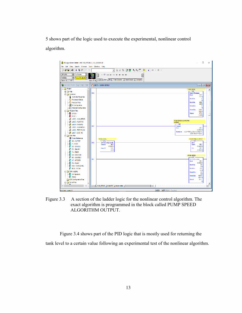
13

5 shows part of the logic used to execute the experimental, nonlinear control

algorithm.

Figure 3.3 A section of the ladder logic for the nonlinear control algorithm. The

exact algorithm is programmed in the block called PUMP SPEED

ALGORITHM OUTPUT.

Figure 3.4 shows part of the PID logic that is mostly used for returning the

tank level to a certain value following an experimental test of the nonlinear algorithm.

14

Figure 3.4 A section of the ladder logic for PID control of the pump. This logic is

executed mostly to return the sump level to a certain value following an

experimental test run.

The version of programming software works by using memory addresses in the

controller to assign values and execute logic. The user must assign the type of

variable, such as an integer, a bit or a floating-point value. For example, an address

shown in Figure 3.4, N7:0, is the value of the sump level stored as an integer value.

The analog values have 12-bit resolution, so N7:0 can range anywhere from 0-4096.

For the pump frequency signal coming to the PLC, the value of frequency between 0

and 60 Hz, is scaled to a value between 0-4096.

15

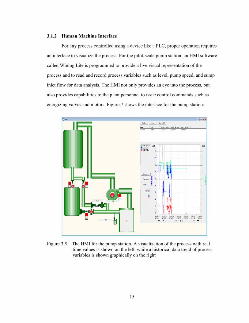
3.1.2 Human Machine Interface

For any process controlled using a device like a PLC, proper operation requires

an interface to visualize the process. For the pilot-scale pump station, an HMI software

called Winlog Lite is programmed to provide a live visual representation of the

process and to read and record process variables such as level, pump speed, and sump

inlet flow for data analysis. The HMI not only provides an eye into the process, but

also provides capabilities to the plant personnel to issue control commands such as

energizing valves and motors. Figure 7 shows the interface for the pump station:

Figure 3.5 The HMI for the pump station. A visualization of the process with real

time values is shown on the left, while a historical data trend of process

variables is shown graphically on the right

16

The process variable data trends shown in Figure 3.5 are a result of a Modbus

RTU communication between the HMI software and the controller. Commands are

issued from the software to read particular analog points that correspond to the correct

process variables and those values are recorded and displayed in the HMI

continuously. The HMI in this case is known as the Modbus master, while the PLC is

the Modbus slave, only capable of receiving commands from the HMI.

3.1.3 System Characteristics

Fittings in the pipe system include a full-bore manual ball valve, a swing check

valve, a globe valve on the discharge side used for introducing frictional resistance

into the system, as well as several 90-degree elbows. An integral flow meter is also

located on the discharge side, which records the total flow produced by the pump for a

given experimental cycle.

A simulated pump/system curve was created using AFT Fathom, a steady-state

fluid mechanics software used for modelling incompressible flow. The curve is

developed with the pump manufacture’s data and interpolation at variable speeds, with

the system curve created for a sump tank level of 58 centimeters (20 inches). Based on

the efficiency curves, it is found that all operating points from 30-60 Hz lie within ±

10% of the Best Efficiency Point (BEP) at a given speed. This figure is shown below:

17

Figure 3.6 (a) Simulated variable speed pump curves for the experiment, with the

system curve developed for Level=50.8 cm (20 in.) and (b) Pump

efficiencies at variable speeds

Inlet flow to the sump comes from the 189 liter (50 gallon) tank, as well as a

95 liter (25 gallon) tank that allows for simulating peak flow rates. Flow rate is

modulated with two on-off valves, as well as a proportional analog control valve that

also receives a 0-10V analog signal from the PLC. A picture of the pilot scale station

is shown below in Figure 3.7.

18

Figure 3.7 The pilot-scale pump station

The PLC programming software was used to control all process parameters,

including pump control algorithms and sump inlet flow rate. Process data was

collected via serial communication and sent to a Human Machine Interface (HMI) for

viewing and analysis. Pump power consumption was recorded through a plug load

logger at an interval of one second and is also collected via data collection software.

19

At the end of every flow cycle, the sump tank level is returned to a predetermined

value, and the next cycle commences.

3.2 Proposed Algorithm

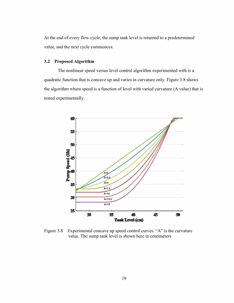
The nonlinear speed versus level control algorithm experimented with is a

quadratic function that is concave up and varies in curvature only. Figure 3.8 shows

the algorithm where speed is a function of level with varied curvature (A value) that is

tested experimentally.

Figure 3.8 Experimental concave up speed control curves. “A” is the curvature

value. The sump tank level is shown here in centimeters

20

The linear functional relationship (A=0) is shown first, with increasing A

values listed below consecutively. For this experimental setup, since the sump tank

maximum height is 50.8 centimeters (20 inches) and the maximum pump speed is

60Hz, the following linear speed versus level control function is created:

1.2*LS L (3.1)

where LS is equal to linear speed and L is the sump tank level in centimeters.

The curves are created by specifying the desired endpoints, and then adding

them to the linear control function. The defining characteristic of each quadratic,

which is the curvature, is defined as the A value, which is listed as experimental

constants in Equation (3.2):

𝐴 = [0 2.5 7.5 10 12.5 15] (3.2)

2

1 2

2 2

AB

L L

(3.3)

where B is equal to a constant, and L1 and L2 are the points where the curve

will intersect the x axis, and where the speed curve will intersect the linear speed

versus level function.

The equation of the curve C is based on the values of A and B and is shown in

Equation (3.4):

2

1 2*2

L LC A B L

(3.4)

21

To get the actual speed versus level control curve, C is added to the linear

speed LS, to come up with the actual speed curve S, shown in Equation (7).

2

1 21.2* *2

L LS L A B L

(3.5)

The values of L1 and L2 can be chosen based on the physical constraints of

any given setup. For the purpose of this experiment, they are chosen as 27.9 cm (11

inches) and 48.3 cm (19 inches) respectively. For A values greater than 5, there exist

points where the derivative of the curve is negative and the speed actually decreases

with increasing level. These points are rejected, and the last known value with a non-

negative derivative is held indefinitely. Since the level endpoint L1 is 27.9 cm, if the

level falls below this value, the calculated pump speed will be held indefinitely with

no further decrease in speed. No pump speed values less than 27.5Hz are considered in

the experiment; in wastewater plants, a minimum speed is generally established to

protect against clogging from solid materials in the sump.

The algorithm itself is created and then implemented using PLC ladder logic

programming, where the liquid level measurement is the input and the pump speed is

the output. The design of the control algorithm consists of specifying the level

endpoints, L1 and L2, and choosing an A value that maximizes the system efficiency

based on the characteristics of the individual pumping system. Essentially, the value of

A can be tuned in order to maximize system efficiency. Since there is no actual level

set-point, there is no error input to the algorithm and therefore no additional design

parameters are considered.

22

3.3 Test Flow Regime

The experiments consist of a test flow regime over a period of 1800 seconds,

where the inlet flow to the sump is controlled to meet a dynamic flow set point. This

flow regime is repeated for each test cycle. Figure 6 shows flow data collected during

one of the cycles to show what the flow regime looks like over an 1800 second period.

Noise looking features in the data are a result of oscillatory behavior of the analog

control valve.

Figure 3.9 Sump inlet flow rate (liters/min) as a function of time for one

experimental cycle. This exact flow regime is repeated for all cycles.

23

Chapter 4

RESULTS AND DISCUSSION

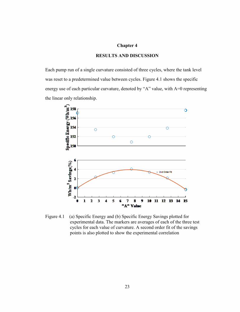
Each pump run of a single curvature consisted of three cycles, where the tank level

was reset to a predetermined value between cycles. Figure 4.1 shows the specific

energy use of each particular curvature, denoted by “A” value, with A=0 representing

the linear only relationship.

Figure 4.1 (a) Specific Energy and (b) Specific Energy Savings plotted for

experimental data. The markers are averages of each of the three test

cycles for each value of curvature. A second order fit of the savings

points is also plotted to show the experimental correlation

24

Table 4.1: Experimental SE Values and % Savings

The specific energy roughly follows a second order parabolic relationship with

a minimum at A=7.5. Using an A value of 15 actually leads to an increase in specific

energy compared to linear control, indicating that there is an optimum curvature to the

algorithm somewhere between A=0 and 15.

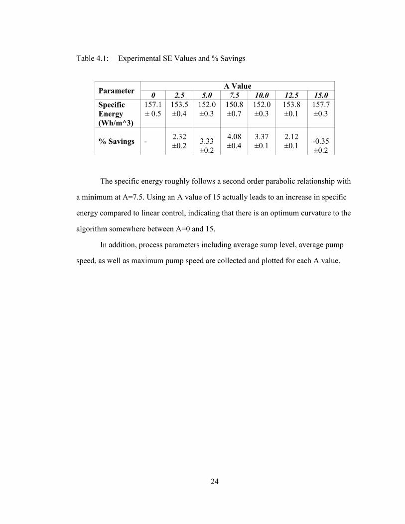
In addition, process parameters including average sump level, average pump

speed, as well as maximum pump speed are collected and plotted for each A value.

Parameter A Value

0 2.5 5.0 7.5 10.0 12.5 15.0

Specific

Energy

(Wh/m^3)

157.1

± 0.5

153.5

±0.4

152.0

±0.3

150.8

±0.7

152.0

±0.3

153.8

±0.1

157.7

±0.3

% Savings - 2.32

±0.2

3.33

±0.2

4.08

±0.4

3.37

±0.1

2.12

±0.1

-0.35

±0.2

25

Figure 4.2 (a) Average Level, (b) Speed and (c) Maximum Speed collected from

data for each curvature value. Each marker represents the average of

three test cycles for the corresponding curvature value.

As shown, while average speed is lower for A=15 than A=0, the maximum

speed is substantially higher. The amount of time spent operating at speeds in excess

of 50 Hz is highlighted in Figure 4.3.

26

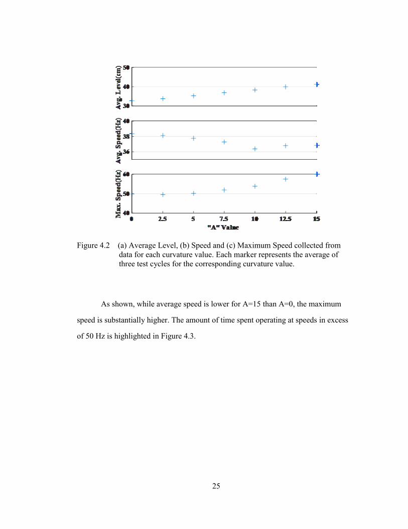
Figure 4.3 (a) Pump Speed, (b) Sump Level and (c) Inlet Flow Rate collected over

the cycle time of 1800 seconds for each curvature value. Each line

represents the average of three test cycles at that particular instance.

It is apparent from the speed versus time results that as the A value increases,

the absolute maximum recorded speed increases. However, for A values greater than

7.5, the duration of operation at high speeds increases substantially. For A=15, when

flow rate reaches one of its four peaks, the speed increases to above 50Hz for a total of

178 seconds on average, substantially more than the 23 seconds for A=7.5. Based on

the affinity laws, since pump power increases cubically with speed, the energy use

increases drastically during periods of high flow due to the pump operating at really

27

high speeds for an extended duration. At the minimum specific energy value of A=7.5,

while the absolute maximum speed (51.9 Hz) was higher than that for A=0 (49.9 Hz),

the duration of operation at the maximum speed was comparatively small, and the

reduced speed during times of lower inlet flow resulted in significant specific energy

savings compared to the linear control. The total operational time at speeds of greater

than 45Hz was 248 seconds for A=0, 196 seconds for A=7.5, and 313 seconds for

A=15. The same trends can be seen in Figure 11, where active power consumption is

monitored over time.

Figure 4.4 Active Power plotted for linear and curvature values of 7.5 and 15

28

Table 4.2: Experimental Process Parameter Values

While active power consumption for A=15 remains less than that of A=7.5 and

A=0 for more than 80% of the cycle duration, the power reaches values in excess of

500 W during the inflow peaks, which actually consumes enough to end up with more

energy drawn during the whole cycle compared to the A=0 algorithm. For A=7.5, the

peak power actually is only slightly more than that of A=0 and integrated over the

whole 1800 seconds and divided by total flow produced, leads to a substantially lower

specific energy compared to the A=0, on the order of 4% less.

Parameter A Value

0 2.5 5.0 7.5 10.0 12.5 15.0

Avg. Tank

Level (cm)

32.73±

0.03

33.73 ±

0.09

35.30

± 0.04

36.81

± 0.13

38.31

± 0.05

39.98 ±

0.03

41.24

±0.05

Avg. In. Flow

Rate

(lpm)

24.19

±0.07

24.18

±0.02

24.05

±0.03

23.95

±0.01

23.77

±0.01

23.65

±0.05

23.48

±0.04

Avg. Pump

Speed

(Hz)

38.36

±0.06

38.12

±0.09

37.78

±0.04

37.26

±0.07

36.41

±0.06

36.79

±0.07

36.83

±0.09

Max. Pump

Speed

(Hz)

49.85

±0.07

49.60

±0.10

50.20

±0.05

51.90

±0.08

53.80

±0.07

57.57

±0.08

60.00

±0.10

Total Pumped

Flow

(m^3/cycle)

0.8121

±

0.0006

0.807 ±

0.003

0.801

±

0.001

0.794

±

0.001

0.787

±

0.001

0.778 ±

0.0006

0.7693

± 0.002

29

Chapter 5

CONCLUSION

This paper has examined an energy efficient control algorithm for pump stations

tasked with controlled sump level, and has presented experimental results showing

specific energy reduction in excess of 4% compared with conventional, linear variable

level control. While the exact amount of savings will depend on specific pump station

parameters, the experimental data shows that there is savings from varying pump

speed nonlinearly with level, and that there is an optimum concave up curve that

produces the most reduction in specific energy.

30

REFERENCES

[1] Goldstein, R., and Smith, W. (2002). “Water & sustainability (Vol. 4): U.S.

electricity consumption for water supply & treatment—The next half century.”

Technical Rep., Electric Power Research Institute (EPRI), Palo Alto, CA.J.

Clerk Maxwell, A Treatise on Electricity and Magnetism, 3rd ed., vol. 2.

Oxford: Clarendon, 1892, pp.68–73.

[2] I. Bakman, L. Gevorkov and V. Vodovozov, "Predictive control of a variable-

speed multi-pump motor drive," 2014 IEEE 23rd International Symposium on

Industrial Electronics (ISIE), Istanbul, 2014, pp. 1409-1414.K. Elissa, “Title of

paper if known,” unpublished.

[3] Y. Tang and S. Zhang, "A Model Predictive Control Approach to Operational

Efficiency of Intake Pump Stations," 2010 International Conference on

Electrical and Control Engineering,

[4] Zhang, Zijun & Zeng, Yaohui & Kusiak, A. (2012). Minimizing pump energy

in a wastewater processing plant. Energy. 47. 505–514.

10.1016/j.energy.2012.08.048.

[5] FLYGT, a xylem brand (2013). Variable speed wastewater pumping. White

Paper, Retrieved from

http://www.wioa.org.au/operator_resources/documents/XylemVariableSpeedP

umping.pdf

31

Appendix

MATLAB CODE

Matlab code for:

Pump Speed Algorithm Curves

Power Data

Speed Data

Level Data

32

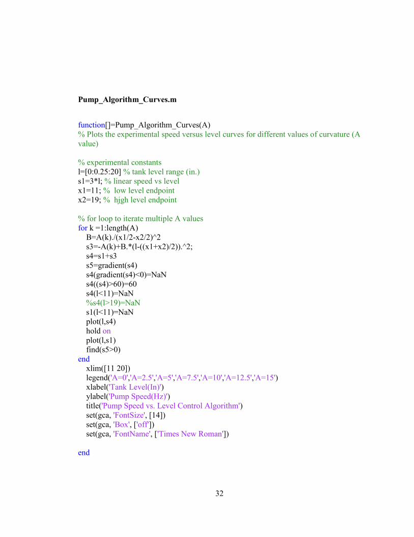
Pump_Algorithm_Curves.m

function[]=Pump_Algorithm_Curves(A)

% Plots the experimental speed versus level curves for different values of curvature (A

value)

% experimental constants

l=[0:0.25:20] % tank level range (in.)

s1=3*l; % linear speed vs level

x1=11; % low level endpoint

x2=19; % hjgh level endpoint

% for loop to iterate multiple A values

for k =1:length(A)

B=A(k)./(x1/2-x2/2)^2

s3=-A(k)+B.*(l-((x1+x2)/2)).^2;

s4=s1+s3

s5=gradient(s4)

s4(gradient(s4)<0)=NaN

s4((s4)>60)=60

s4(l<11)=NaN

%s4(l>19)=NaN

s1(l<11)=NaN

plot(l,s4)

hold on

plot(l,s1)

find(s5>0)

end

xlim([11 20])

legend('A=0','A=2.5','A=5','A=7.5','A=10','A=12.5','A=15')

xlabel('Tank Level(In)')

ylabel('Pump Speed(Hz)')

title('Pump Speed vs. Level Control Algorithm')

set(gca, 'FontSize', [14])

set(gca, 'Box', ['off'])

set(gca, 'FontName', ['Times New Roman'])

end

33

POWER_Data.m

% Experiment_Pumping Power Data for Pilot Scale Station

% Pump Power Data is taken for variable curvature(A value)Speed vs. Level

%% Excel Data

% Each curavture (A value) has 3 experimental cycles:

% A=0

dataset=xlsread('A=0(average).xlsx','A=0(2)','C2:C1801');%A=0

dataset2=xlsread('A=0(average).xlsx','A=0(3)','C2:C1801');%A=0

dataset3=xlsread('A=5,A=7.5(average).xlsx','Pump_Station_17','C10857:C12656');%

A=0

% A=5

dataset4=xlsread('A=5(new average).xlsx','Pump_Station_19','C3:C1802');%A=5

dataset5=xlsread('A=5(new average).xlsx','Pump_Station_19','C1813:C3612');%A=5

dataset6=xlsread('A=5(new average).xlsx','Pump_Station_19','H3:H1802');%A=5

% A=7.5

dataset7=xlsread('A=7.5_new_average.xlsx','Pump_Station_21','C3:C1802');%A=7.5

dataset8=xlsread('A=7.5_new_average.xlsx','Pump_Station_21','J3:J1802');%A=7.5

dataset9=xlsread('A=7.5_new_average.xlsx','Pump_Station_21','P3:P1802');%A=7.5

% A=10

dataset10=xlsread('A=10,A=2.5(average).xlsx','Pump_Station_18','C3:C1802');%A=1

0


A=10


A=10

% A=2.5


A=2.5


A=2.5

34


A=2.5

% A=12.5

dataset16=xlsread('A=12.5.xlsx','Pump_Station_22','C3:C1802');%A=12.5

dataset17=xlsread('A=12.5.xlsx','Pump_Station_22','C1813:C3612');%A=12.5

dataset18=xlsread('A=12.5.xlsx','Pump_Station_22','I3:I1802');%A=12.5

% A=15

dataset19=xlsread('A=15.xlsx','Pump_Station_25','C3:C1802');%A=15



%%

%% Mean Active Power (W)

pdmean=(dataset+dataset2+dataset3)/3;

pdemean2=(dataset4+dataset5+dataset6)/3;






x=[1:1800] % Array spanning length of dataset for plotting purposes

% For example sake, I overwrote values of power for times where the pump was

turned off

pdmean(pdmean<200)=200

pdemean3(pdemean3<190)=190

%%

%% Converting to Specific Energy

% Trapz takes integral under power data to get energy [Wh]

% Divide by total value of pumped flow to get specific energy [Wh/gallon]

% Convert to metric units for publication in Canada [Wh/m^3]

me=264.17 %gpm to m3/m

%A=0

energy = trapz(dataset)/(3600*214.71/me)

energy2 = trapz(dataset2)/(3600*214.5/me)


35

%A=5




%A=7.5




%A=10


energy11 = trapz(dataset11)/(3600*208/me)


%A=2.5




%A=12.5




%A=15




%Specific Energy Arrays

SE=[energy energy2 energy3] %A=0

SE2=[energy4 energy5 energy6] %A=5

SE3=[energy7 energy8 energy9] %A=7.5





%% Average, %Savings, and STD for different values of Curvature

% Average of Specific Energy

Avg=[mean(SE) mean(SE5) mean(SE2) mean(SE3) mean(SE2) mean(SE6)

mean(SE7)]

% %Savings of Specific Energy

savings=[0 (mean(SE)-mean(SE5))/((mean(SE)+mean(SE5))/2)*100 (mean(SE)-

mean(SE2))/((mean(SE)+mean(SE2))/2)*100 (mean(SE)-


36



mean(SE7))/((mean(SE)+mean(SE7))/2)*100]

% STD of Specific Energy

STD2=[0 std((SE)) std((SE5)) std((SE2)) std((SE3)) std((SE2)) std((SE6)) std((SE7))]

A=[0 2.5 5 7.5 10 12.5 15]

% Subplot 1 is average specific energy for each value of curvature

subplot(2,1,1)

plot(A,Avg,'o')

hold on

ylabel('Specific Energy (Wh/m^3)')




set(gca, 'XTick', [])

set(gcf, 'Color', [1 1 1])

set(gca, 'YGrid', 'on')

set(gca, 'LineWidth', [2.000])

% Subplot 2 is the %savings of each curvature compared to the linear one(A=0)

% Added a polyfit curve just to illustrate how the data is follow a trend

subplot(2,1,2)

plot(A,savings,'o')

P=polyfit(A,savings,2)

x1=linspace(0,15)

y1=polyval(P,x1)

hold on

plot(x1,y1)

xlabel('"A" Value','fontsize',18)




set(gca, 'XTick', [0 1 2 3 4 5 6 7 8 9 10 11 12 13 14 15])

set(gca, 'LineWidth', [2.000])

text(11,3.5,'\leftarrow 2nd Order Fit','FontSize',8,'FontWeight','bold')

ylabel('Wh/m^3 Savings(%)','fontsize',14)

%%

37

SPEED_data.m

sdataset=xlsread('A=0(average).xlsx','A=0(2)','E2:E1801');%A=0

sdataset2=xlsread('A=0(average).xlsx','A=0(3)','E2:E1801');%A=0

sdataset3=xlsread('A=5,A=7.5(average).xlsx','Pump_Station_17','C10857:C12656');%

A=0

sdataset4=xlsread('A=5(new average).xlsx','Pump_Station_19','E3:E1802');%A=5

sdataset5=xlsread('A=5(new average).xlsx','Pump_Station_19','E1813:E3612');%A=5

sdataset6=xlsread('A=5(new average).xlsx','Pump_Station_19','J3:J1802');%A=5

sdataset7=xlsread('A=7.5_new_average.xlsx','Pump_Station_21','L3:L1802');%A=7.5

sdataset8=xlsread('A=7.5_new_average.xlsx','Pump_Station_21','E3:E1802');%A=7.5

sdataset9=xlsread('A=7.5_new_average.xlsx','Pump_Station_21','R3:R1802');%A=7.5

sdataset10=xlsread('A=10,A=2.5(average).xlsx','Pump_Station_18','E3:E1802');%A=1

0

sdataset11=xlsread('A=10,A=2.5(average).xlsx','Pump_Station_18','E1813:E3612');%

A=10


A=10


A=2.5


A=2.5

sdataset15=xlsread('A=10,A=2.5(average).xlsx','Pump_Station_18','E9053:E10852');

%A=2.5

sdataset16=xlsread('A=12.5.xlsx','Pump_Station_22','E3:E1802');%A=12.5

sdataset17=xlsread('A=12.5.xlsx','Pump_Station_22','E1813:E3612');%A=12.5

sdataset18=xlsread('A=12.5.xlsx','Pump_Station_22','K3:K1802');%A=12.5

sdataset19=xlsread('A=15.xlsx','Pump_Station_25','E3:E1802');%A=12.5



sdmean=(sdataset+sdataset2)/2;

sdemean2=(sdataset4+sdataset5+sdataset6)/3;





38


sdmean(sdmean<30)=NaN

x=[1:1800]

%subplot(2,1,1)

%plot(x,dataset,x,dataset2,x,dataset3)

%legend('Linear(A=0)','Conc. Up(A=5)','Conc. Up(A=-6.5)')

xlabel('Time(s)')

ylabel('Pump Speed(Hz)')

%title('Pump Energy Data')



%text(10,500,'Spec. E =0.5979 wH','FontSize',8)

%text(10,475,'Spec. E=0.5832 wH','FontSize',8)


%subplot(2,1,2)

%A=0

speed = mean(sdataset)

speed2 = mean(sdataset2)


%A=5




%A=7.5




%A=10




%A=2.5




%A=12.5




%A=15



39


Sp=[speed speed2] %A=0

Sp2=[speed4 speed5 speed6] %A=5

Sp3=[speed7 speed8 speed9] %A=7.5





STD=[std(Sp) std(Sp5) std(Sp2) std(Sp3) std(Sp4) std(Sp6) std(Sp7)]

Avgs=[mean(Sp) mean(Sp5) mean(Sp2) mean(Sp3) mean(Sp4) mean(Sp6)

mean(Sp7)]

%max=[max(dataset) max(dataset15) max(dataset4) max(dataset7) max(dataset10)

max(dataset16) max(dataset19)]

Max=[max(sdmean),max(sdemean5),max(sdemean2),max(sdemean3),max(sdemean4)

,max(sdemean6),60]

%savings=[0 (mean(SE)-mean(SE5))/((mean(SE)+mean(SE5))/2)*100 (mean(SE)-





mean(SE7))/((mean(SE)+mean(SE7))/2)*100]

A=[0 2.5 5 7.5 10 12.5 15]

J=find(sdemean3>=45)

i=length(J)

H=find(sdmean>=45)

i2=length(H)

%P=polyfit(A,savings,2)

%x1=linspace(0,15)

%y1=polyval(P,x1)

subplot(3,1,1)

plot(A,AvgL,'+')

%plot(x,sdmean,x,sdemean2,x,sdemean3,x,sdemean4,x,sdemean5,x,sdemean6,x,sdem

ean7)

%hold on

%plot(x1,y1)

%legend('SE Savings','2nd Degree Fit')

ylabel('Avg. Level(cm)','fontsize',12)

%title('Specific Energy Savings')

%set(gca, 'FontSize', [15])

set(gca, 'FontWeight', ['bold'])


40


%set(gca, 'XTick', [0 300 600 900 1200 1500 1800])



set(gcf, 'Color', [1 1 1])

subplot(3,1,2)

plot(A,Avgs,'+')

%xlabel('"A" Value')

ylabel('Avg. Speed(Hz)','fontsize',12)






ylim([35 40])


subplot(3,1,3)

plot(A,Max,'+')

xlabel('"A" Value','fontsize',18)

ylabel('Max. Speed(Hz)','fontsize',12)





set(gca, 'XTick', [0 2.5 5.0 7.5 10.0 12.5 15.0])


41

LEVEL_data.m

%% Sump Tank Level Data taken for different values of Curvature (A Value)

%% Sump Tank Level Data pulled from Excel

% 3 datasets for each value of curvature (Each pump cycle is 1800 seconds)

% 2.54 converts inches to centimeters

% A=0

ldataset=2.54*xlsread('A=0(average).xlsx','A=0(2)','D2:D1801');%A=0

ldataset2=2.54*xlsread('A=0(average).xlsx','A=0(3)','D2:D1801');%A=0

% ldataset3 excel data is corrupted, just ignored it.

% A=5

ldataset4=2.54*xlsread('A=5(new

average).xlsx','Pump_Station_19','D3:D1802');%A=5

ldataset5=2.54*xlsread('A=5(new

average).xlsx','Pump_Station_19','D1813:D3612');%A=5

ldataset6=2.54*xlsread('A=5(new average).xlsx','Pump_Station_19','I3:I1802');%A=5

% A=7.5

ldataset7=2.54*xlsread('A=7.5_new_average.xlsx','Pump_Station_21','K3:K1802');%

A=7.5

ldataset8=2.54*xlsread('A=7.5_new_average.xlsx','Pump_Station_21','D3:D1802');%

A=7.5

ldataset9=2.54*xlsread('A=7.5_new_average.xlsx','Pump_Station_21','Q3:Q1802');%

A=7.5

% A=10

ldataset10=2.54*xlsread('A=10,A=2.5(average).xlsx','Pump_Station_18','D3:D1802');

%A=10

ldataset11=2.54*xlsread('A=10,A=2.5(average).xlsx','Pump_Station_18','D1813:D361

2');%A=10


2');%A=10

42

% A=2.5


2');%A=2.5


2');%A=2.5


52');%A=2.5

% A=12.5

ldataset16=2.54*xlsread('A=12.5.xlsx','Pump_Station_22','D3:D1802');%A=12.5

ldataset17=2.54*xlsread('A=12.5.xlsx','Pump_Station_22','D1813:D3612');%A=12.5

ldataset18=2.54*xlsread('A=12.5.xlsx','Pump_Station_22','J3:J1802');%A=12.5

% A=15

ldataset19=2.54*xlsread('A=15.xlsx','Pump_Station_25','D3:D1802');%A=15



%%

%% Mean Level Dataset

lsdmean=(ldataset+ldataset2)/2;

lsdemean2=(ldataset4+ldataset5+ldataset6)/3;






%%

%plot(x,lsdmean,x,lsdemean2,x,lsdemean3,x,lsdemean4,x,lsdemean5,x,lsdemean6,x,l

sdemean7)

%x=[1:1800]

%subplot(2,1,1)

%plot(x,dataset,x,dataset2,x,dataset3)

%legend('Linear(A=0)','Conc. Up(A=5)','Conc. Up(A=-6.5)')

xlabel('Time(s)')

ylabel('Power(W)')

title('Pump Energy Data')



%text(10,500,'Spec. E =0.5979 wH','FontSize',8)



%subplot(2,1,2)

43

%A=0

%% Average Level during each Pumping Cycle for given Curvature Value

% A=0

level = mean(ldataset)

level2 = mean(ldataset2)

% A=5




% A=7.5




% A=10




% A=2.5




% A=12.5




% A=15




SEl=[level level2] %A=0

SEl2=[level4 level5 level6] %A=5

SEl3=[level7 level8 level9] %A=7.5





44

%%

%% Average Level and STD

STD=[std(SEl) std(SEl5) std(SEl2) std(SEl3) std(SEl4) std(SEl6) std(SEl7)]

AvgL=[mean(SEl) mean(SEl5) mean(SEl2) mean(SEl3) mean(SEl4) mean(SEl6)

mean(SEl7)]

A=[0 2.5 5 7.5 10 12.5 15]

%Plot of Average Sump Level for value of Curvature

plot(A,AvgL,'+')

xlabel('"A" Value')

ylabel('Avg. Tank Level(cm)')




set(gca, 'XTick', [0 2.5 5.0 7.5 10.0 12.5 15.0])

%%

INVESTIGATION OF AN ENERGY EFFICIENT PUMP SPEED …

Documents

Transcript of INVESTIGATION OF AN ENERGY EFFICIENT PUMP SPEED …