Investigation into the effect of stripped gas liquor on ...

Investigation into the effect of stripped gas liquor

on the anaerobic digestion of Fischer-Tropsch reaction water

SCHOOL OF CHEMICAL ENGINEERING

HOWARD COLLEGE

Renésha Roopan

208504705

Submitted in fulfilment of the academic

requirements for the degree of

Master of Science

in the School of Chemical Engineering,

University of KwaZulu-Natal, Durban

March 2014

Supervisor: Dr K.M. Foxon

Pollution Research Group

As the candidate’s Supervisor I agree/ do not agree to the submission of this dissertation.

…………………………………… ……………………………..

Dr K.M. Foxon (Supervisor) Date

…………………………………… ……………………………..

Renésha Roopan (Student) Date

i

Declaration

I, Renésha Roopan, declare that

(i) The research reported in this dissertation, except where otherwise indicated, is my

original work

(ii) This dissertation has not been submitted for any degree or examination at any

other university

(iii) This dissertation does not contain other persons’ data, pictures, graphs or other

information, unless specifically acknowledged as being sourced from other

persons

(iv) This dissertation does not contain other persons’ writing, unless specifically

acknowledged as being sourced from other researchers.

Where other written sources have been quoted, then:

a) Their words have been re-written but the general information attributed to

them has been referenced;

b) Where their exact words have been used, their writing has been placed inside

quotation marks, and referenced.

(v) Where I have reproduced a publication of which I am an author, co-author or

editor, I have indicated in detail which part of the publication was actually written

by myself alone and have fully referenced such publications.

(vi) This dissertation does not contain text, graphics or tables copied and pasted from

the Internet, unless specifically acknowledged, and the source being detailed in

the dissertation and in the References sections.

…………………………………… ……………………………..

Renésha Roopan Date

ii

Acknowledgements

I would like to thank the following people for their integral contribution to the successful

completion of this Master of Science project:

My supervisor, Dr K.M. Foxon, for her support, advice and guidance throughout the

duration of this project and the many hours spent checking and rechecking my work.

My co-supervisor, Mr C. Brouckaert and the Head of the Pollution Research Group,

Prof C. Buckley for their invaluable input and advice.

Sasol Technology R&D, Environmental Science and Engineering and National

Research Foundation for the financing of the project.

The members of Sasol Technology R&D, Environmental Science and Engineering for

their vital feedback.

The workshop staff at the School of Chemical Engineering for the building of the

set-up used in the experiments of this project.

Merlien Reddy and the technical support staff at the School of Chemical Engineering

for their expansive help with the use of lab equipment.

Researchers who helped extensively with the research and experiments for this

project, including Daniel Teclu, Bjoern Pietruschka and Nicolette Govender.

Kevin Wickee for the training for the use of the gas chromatograph, as well as, the

maintanence and repairs of the gas chromatograph.

My family, mum, dad and sister, and friends who have supported me in countless

ways throughout this project. Thank you for your faith, support and love.

iii

Abstract

The Fischer-Tropsch reaction technology is utilised in Sasol’s Coal-to-liquid plant to produce

liquid fuels from low grade coal. There are several processes on the Coal-to-liquid plant that

generate aqueous streams which contain a high organic load and require treatment. The main

contributors to the wastewater are the Phenosolvan plant, producing stripped gas liquor

(SGL), and the Synthol plant, producing Fischer-Tropsch reaction water (FTRW). Stripped

gas liquor contains water, organic acids, ammonia, and potentially toxic phenols.

Fischer-Tropsch reaction water contains volatile fatty acids and alcohol. Stripped gas liquor

is therefore nitrogen-rich while FTRW is nitrogen-deficient and requires nutrient

supplementation for anaerobic treatment. Therefore co-treatment of the two streams could

reduce nitrogen supplementation requirements.

This study is part of a larger project to determine the feasibility of anaerobically co-digesting

FTRW and SGL.

This study has looked at the influence of SGL on the methanogenic activity of

FTRW-acclimated sludge and involved the development of a method which allows accurate

recording of the methanogenic activity in batch assays. Other studies involving the anaerobic

digestion of high phenolic wastewaters showed that the phenol had an inhibitory effect on the

specific methanogenic activity of the sludge, which was not acclimated to the phenol. The

objective of this work was to test the hypotheses that (1) anaerobic sludge acclimated to

FTRW will be inhibited by high molecular weight organics in SGL and

(2) FTRW-acclimated sludge will not degrade phenolic compounds in SGL. This information

will be used for designing process configurations for simultaneous treatment of the two

streams with minimum contamination of the effluent stream.

The serum bottle was used as a small batch reactor and the biogas production was monitored

as an indication of the state of the reaction. The biogas produced was collected and measured

by the downward displacement of a sodium hydroxide solution, which absorbed the carbon

dioxide and collected only the methane. A concentration of 1 g COD/ℓ FTRW was chosen as

the reference test due to the reproducibility of the replicates within each experiment as well

as its reproducibility across different batches of sludge. For the first inhibition test, the test

units contained an additional 5% SGL (0.05 g COD/ℓ SGL) and an additional 15% SGL

(0.15 g COD/ℓ SGL, i.e. 13% of the total COD load) respectively, added to 1 g COD/ℓ

iv

FTRW. The 5% SGL test unit showed no inhibition compared to the reference unit. There

was a reduction in the specific methanogenic activity of the 15% SGL test units compared to

the reference unit. Since the total COD load was not the same in each unit, it cannot be

conclusively stated that the SGL was responsible for the reduction in SMA, but this seems a

reasonable possibility in the light of results from the reference test selection experiments

which showed higher SMA at higher organic loading rates.

For the second inhibition test, the test units contained 85% FTRW (0.85 g COD/ℓ FTRW)

and 15% SGL (0.15 g COD/ℓ SGL) to make up a total COD load of 1 g COD/ℓ. There was

an increase in the specific methanogenic activity of the test unit compared to the reference

unit. There was very little change in the phenol concentration.

Therefore, it was concluded the addition of SGL potentially reduced the SMA and that this

could be an inhibitory effect, but that any inhibition would be a function of the concentration

of potentially inhibitory substances in SGL and that these concentrations vary from batch to

batch. However, the degree of SMA reduction is fairly low and would not prevent

co-digestion of the two streams at the concentrations tested. It has been shown that FTRW

anaerobic digestion can proceed adequately in the presence of SGL. There was some

evidence that phenolics were degraded but at a much slower rate than COD. The percentage

reduction in SMA due to additional SGL at concentrations and SGL:FTRW ratios tested was

between 0 and 51%.

Ultimately, this work is a first step in the development of a co-digestion model relating

organic loading rate, SGL:FTRW feed ratio to methane recovery and extent of

biodegradation of phenol for use in the design and optimization of a co-digestion system.

v

Table of contents

Declaration .................................................................................................................................. i

Acknowledgements .................................................................................................................... ii

Abstract .................................................................................................................................... iii

Table of contents ........................................................................................................................ v

List of figures ............................................................................................................................ ix

List of tables ........................................................................................................................... xiii

List of abbreviations ............................................................................................................... xiv

1. Introduction ........................................................................................................................ 1

1.1. Context of the Study ........................................................................................................ 1

1.2. Significance of the Study ................................................................................................ 4

2. Theory and Literature Review ............................................................................................ 6

2.1. Fischer-Tropsch Reaction Water ..................................................................................... 6

2.2. Stripped Gas Liquor ........................................................................................................ 7

2.3. Anaerobic Digestion ........................................................................................................ 7

2.4. Factors Affecting Anaerobic Digestion......................................................................... 11

2.4.1. Temperature ............................................................................................................ 11

2.4.2. pH ........................................................................................................................... 11

2.4.3. Weak acids and bases ............................................................................................. 12

2.4.4. Nutrients ................................................................................................................. 12

2.5. Co-digestion .................................................................................................................. 12

2.6. Inhibition ....................................................................................................................... 13

2.7. Serum Bottle Test .......................................................................................................... 14

2.8. Biogas measurement techniques ................................................................................... 15

2.9. Anaerobic Digestion of High Alcohol Wastewaters ..................................................... 16

2.10. Anaerobic Digestion of High Phenolic Wastewaters and Phenolic Compounds ........ 17

2.11. Summary ..................................................................................................................... 19

3. Experiment Design ........................................................................................................... 22

3.1. Hypotheses .................................................................................................................... 22

3.2. Research Outcomes ....................................................................................................... 23

3.3. Overview of Experiment Design ................................................................................... 23

3.4. Materials ........................................................................................................................ 24

3.4.1. Sludge ..................................................................................................................... 24

vi

3.4.2. Substrates ................................................................................................................ 24

3.4.3. Nutrients ................................................................................................................. 25

3.5. Physicochemical Characteristics of Substrates and Sludge .......................................... 26

3.5.1. pH test ..................................................................................................................... 26

3.5.2. Alkalinity test ......................................................................................................... 26

3.5.3. Solids test ................................................................................................................ 26

3.5.4. Chemical oxygen demand test ................................................................................ 27

3.6. Serum Bottle Test .......................................................................................................... 28

3.7. Gas Composition Measurement .................................................................................... 28

3.8. Phenol Measurement ..................................................................................................... 29

3.8.1. Colorimetric method ............................................................................................... 29

3.8.2. Gas chromatography ............................................................................................... 31

3.9. Data Interpretation......................................................................................................... 31

3.9.1. Cumulative volume ................................................................................................. 31

3.9.2. Net methane volume ............................................................................................... 33

3.9.3. Conversion of moles of methane to COD .............................................................. 33

3.9.4. Conversion of COD to volume of methane ............................................................ 34

3.9.5. Percentage COD recovery ...................................................................................... 34

3.9.6. Specific methanogenic activity (SMA) .................................................................. 35

3.9.7. Inhibition ................................................................................................................ 36

3.10. Statistical Methods ...................................................................................................... 37

3.10.1. Confidence limits for a mean................................................................................ 37

3.10.2. Difference between two means ............................................................................. 37

3.10.3. Paired two sample t-test ........................................................................................ 38

4. Method Development ....................................................................................................... 39

4.1. Water Displacement Method ......................................................................................... 39

4.1.1. Proof of concept...................................................................................................... 42

4.1.2. Set 1: Testing the water displacement method with FTRW and UASB 1 sludge .. 44

4.2. Acidified Brine Solution Method .................................................................................. 45

4.2.1. Set 2: Testing the acidified brine solution displacement method with FTRW and

UASB 1 sludge ................................................................................................................. 46

4.2.2. Set 3: Testing the necessity of additional nutrient supplementation ...................... 47


UASB 2 sludge ................................................................................................................. 49

vii

4.2.4. Advantages and disadvantages of the acidified brine solution displacement method

.......................................................................................................................................... 51

4.3. Alkaline Solution Method ............................................................................................. 52

4.3.1. Set 5: Comparison of the acidified brine solution method to the alkaline solution

method .............................................................................................................................. 54

4.3.2. Advantages and disadvantages of the alkaline solution method ............................ 57

4.4. Reference Test ............................................................................................................... 57

4.4.1. Set 6 ........................................................................................................................ 57

4.4.2. Set 7 ........................................................................................................................ 59

4.4.3. Comparing results from different batches of sludge .............................................. 61

4.5. Summary ....................................................................................................................... 65

5. Effect of SGL on FTRW Digestion .................................................................................. 66

5.1. Set 8: Constant FTRW COD load ................................................................................. 67

5.2. Set 9: Constant total COD load ..................................................................................... 72

6. Discussion ......................................................................................................................... 82

6.1. Method development ..................................................................................................... 82

6.1.1. The necessity of additional nutrients ...................................................................... 82

6.1.2. Gas collection techniques ....................................................................................... 83

6.1.3. Reference test ......................................................................................................... 83

6.2. Effect of SGL on FTRW digestion ............................................................................... 84

6.2.1. Constant FTRW COD load (Set 8) ......................................................................... 84

6.2.2. Constant total COD load (Set 9) ............................................................................. 85

6.3. Hypotheses .................................................................................................................... 86

7. Conclusions and Recommendations ................................................................................. 88

7.1. Conclusions ................................................................................................................... 88

7.2. Recommendations ......................................................................................................... 90

References ................................................................................................................................ 91

Appendices ............................................................................................................................... 97

A. Physicochemical characteristics of substrates and sludge ............................................ 97

Sludge and substrates used in sets 1 - 8 ............................................................................ 97

Sludge and substrates used in set 9 ................................................................................... 97

B. Gas chromatograph calibration curves for biogas testing ............................................. 98

C. Proof of concept of water displacement method......................................................... 100

Preparation of stock solution .......................................................................................... 100

viii

Theoretical amount of methane and carbon dioxide produced ....................................... 101

D. Volumes of sludge, nutrients and substrate used in experiments ............................... 102

Set 1: Testing the water displacement method with FTRW and UASB 1 sludge .......... 102

Set 2: Testing the acidified brine solution displacement method ................................... 102

Set 3: Testing the necessity of nutrients ......................................................................... 103

Set 4: Testing the acidified brine solution displacement method with FTRW and UASB 2

sludge .............................................................................................................................. 103

Set 5: Comparison of the acidified brine solution method to the alkaline solution method

........................................................................................................................................ 104

Set 6: COD values of 1, 1.5 and 2 g COD/ℓ ................................................................... 104

Set 7: COD values of 1, 1.5 and 2 g COD/ℓ ................................................................... 105

Set 8: Constant FTRW COD load .................................................................................. 106

Set 9: Constant total COD load ...................................................................................... 107

E. Standard operating procedures .................................................................................... 108

E1. Determination of characteristics of stripped gas liquor, Fischer-Tropsch reaction

water and UASB 1 sludge .............................................................................................. 108

E2. Serum bottle test procedure ...................................................................................... 118

E3. Gas chromatograph calibration and biogas testing .................................................. 120

E4. Phenol measurement ................................................................................................ 121

F. Paired two sample t-test .............................................................................................. 127

G. Percentage inhibition .................................................................................................. 128

ix

List of figures

Figure 1.1: Graph showing an uncalibrated model of co-digestion a labile and inhibitory

substrate (Foxon, unpublished) .................................................................................................. 3

Figure 2.1: Flow diagram of the stages involved in anaerobic digestion (Adapted from

Batstone et al., 2002) ............................................................................................................... 10

Figure 3.1: Diagram of a serum bottle, its components and contents ...................................... 28

Figure 3.2: The reaction of 4-aminoantipyrine with phenol (Emerson, 1943) ........................ 30

Figure 3.3: Representation of A) cumulative biogas volume vs time graphs of the control

(dashed line), reference unit and test unit and B) a net volume of biogas vs time graph (solid

line) (Source: Remigi et al., 2006) ........................................................................................... 32

Figure 3.4: Possible shapes of the graph of cumulative biogas volume vs time (Source:

Remigi et al., 2006) .................................................................................................................. 33

Figure 3.5: Representation of B) specific methanogenic activity vs time graphs and C) the

possible shapes of the graph of specific methanogenic activity vs time (Source: Remigi et al.,

2006) ........................................................................................................................................ 36

Figure 4.1: Set-up of the serum bottle test and water displacement method showing the

dropper arrangement for one of the bottles .............................................................................. 40

Figure 4.2: Photograph of the arrangement of the droppers with the bottom droppers being

the gas collection droppers and the droppers above being the overflow chambers ................. 41

Figure 4.3: Photograph showing the attachment of the serum bottles in the water bath to the

gas collection droppers ............................................................................................................ 41

Figure 4.4: Graph showing the average cumulative net biogas production (mℓ) over time

(days) in trial run 1 ................................................................................................................... 43


(days) in trial run 2 ................................................................................................................... 43

Figure 4.6: Graph showing the average cumulative net biogas produced (mℓ) over time (days)

when food-to-micro-organism ratios of 0.2, 0.25 and 0.3 were used with only Fischer-

Tropsch reaction water as the substrate ................................................................................... 44

Figure 4.7: Graph showing the specific biogas production rate (mℓ/gVSS.day) over time

(days) when food-to-micro-organism ratios of 0.2, 0.25 and 0.3 were used with only Fischer-

Tropsch reaction water as the substrate ................................................................................... 45


(days) with UASB 1 sludge, nutrients and Fischer-Tropsch reaction water as the substrate .. 46


(days) with UASB 1 sludge, nutrients and Fischer-Tropsch reaction water as the substrate .. 47


(days) with UASB 1 sludge and Fischer-Tropsch reaction water as the substrate .................. 48


(days) with UASB 1 sludge and Fischer-Tropsch reaction water as the substrate .................. 48


(days) with UASB 2 sludge and different concentrations of FTRW ....................................... 50

x


(days) with UASB 2 sludge and different concentrations of FTRW ....................................... 50


dropper arrangement for one of the bottles .............................................................................. 52

Figure 4.15: Photograph of the arrangement of the inverted bottles, filled with sodium

hydroxide solution, above the plastic cylinders ....................................................................... 53

Figure 4.16: Photograph of showing the attachment of the serum bottles in the water bath to

the inverted bottles filled with sodium hydroxide solution ..................................................... 53


(days) with UASB 2 sludge and 1 g COD/ℓ of FTRW using the acidified brine solution

method...................................................................................................................................... 54


(days) with UASB 2 sludge and 1 g COD/ℓ of FTRW using the acidified brine solution

method...................................................................................................................................... 55

Figure 4.19: Graph showing the average cumulative net methaneproduction (mℓ) over time

(days) with UASB 2 sludge and 1 g COD/ℓ of FTRW using the alkaline solution method.... 55

Figure 4.20: Graph showing the specific methanogenic activity (mℓ/gVSS.day) over time

(days) with UASB 2 sludge and 1 g COD/ℓ of FTRW using the alkaline solution method.... 56

Figure 4.21: Graph showing the average cumulative net methane production (mℓ) over time

(days) with UASB 2 sludge and 1, 1.5 and 2 g COD/ℓ of FTRW ........................................... 58



Figure 4.23: Graph showing the average cumulative net methane production (mℓ) over time




Figure 4.25: Graph showing the cumulative net methane production (mℓ) over time (days)

from different batches of sludge when 1 g COD/ℓ FTRW is used .......................................... 61


(days) from different batches of sludge when 1 g COD/ℓ FTRW is used ............................... 62


from different batches of sludge when 1.5 g COD/ℓ FTRW is used ....................................... 62


(days) from different batches of sludge when 1.5 g COD/ℓ FTRW is used ............................ 63


from different batches of sludge when 2 g COD/ℓ FTRW is used .......................................... 63


(days) from different batches of sludge when 2 g COD/ℓ FTRW is used ............................... 64

Figure 5.1: Graph showing the average cumulative net methane production (mℓ/gVSS)

against time (days) when only 1 g COD/ℓ of FTRW is degraded and when 1 g COD/ℓ of

FTRW is co-digested with 5% SGL and 15% SGL. Reference units are labelled according to

Table 5-3 .................................................................................................................................. 68

xi

Figure 5.2: Graph showing the percentage COD recovery (%) over time (days) when only 1 g

COD/ℓ of FTRW is degraded and when 1 g COD/ℓ of FTRW is co-digested with 5% SGL

and 15% SGL. Reference units are labelled according to Table 5-3 ....................................... 68

Figure 5.3: Graph showing the average specific methanogenic activity (mℓ/gVSS.day) over

time (days) when only 1 g COD/ℓ of FTRW is degraded and when 1 g COD/ℓ of FTRW is

co-digested with 5% SGL and 15% SGL ................................................................................ 69

Figure 5.4: Graph showing the proposed points and dates at which the extra bottles will be

sacrificed .................................................................................................................................. 73


against time (days) when only 1 g COD/ℓ of FTRW is degraded and when 0.85 g COD/ℓ of

FTRW is co-digested with 0.15 g COD/ℓ of SGL ................................................................... 74

Figure 5.6: Graph showing the percentage COD recovery (%) against time (days) when only

1 g COD/ℓ of FTRW is degraded and when 0.85 g COD/ℓ of FTRW is co-digested with 0.15

g COD/ℓ of SGL ...................................................................................................................... 74

Figure 5.7: Graph showing the specific methanogenic activity (mℓ/gVSS.day) against time

(days) when only 1 g COD/ℓ of FTRW is degraded and when 0.85 g COD/ℓ of FTRW is co-

digested with 0.15 g COD/ℓ of SGL ........................................................................................ 75

Figure 5.8: Graph showing the pH value against time (days) for the test unit with

0.85 g COD/ℓ of FTRW co-digested with 0.15 g COD/ℓ of SGL ........................................... 77

Figure 5.9: Graph showing the volatile suspended solids (mg/ℓ) against time (days) for the

test unit with 0.85 g COD/ℓ of FTRW co-digested with 0.15 g COD/ℓ of SGL ..................... 77

Figure 5.10: Graph showing the COD (mg/ℓ) against time (days) for the test unit with 0.85 g

COD/ℓ of FTRW co-digested with 0.15 g COD/ℓ of SGL ...................................................... 78

Figure 5.11: Graph showing the phenol concentration (mg/ℓ) against time (days) for the test

unit with 0.85 g COD/ℓ of FTRW co-digested with 0.15 g COD/ℓ of SGL ........................... 79

Figure 5.12: Gas chromatograph profile of the test unit showing the phenol peak at the

beginning of the experiment (day 1) ........................................................................................ 80

Figure 5.13: Gas chromatograph profile of the test unit showing the phenol peak at the end of

the experiment (day 23) ........................................................................................................... 80

Figure 5.14: Overlap of the gas chromatograph profiles of the test unit at the beginning

(orange) and end of the experiment (black) ............................................................................. 81

Figure B 1: Graph showing the response of air (mV/s) when different volumes of air (mℓ) are

injected into a gas chromatograph ........................................................................................... 98

Figure B 2: Graph showing the response of nitrogen (mV/s) when different volumes of

nitrogen (mℓ) are injected into a gas chromatograph .............................................................. 98

Figure B 3: Graph showing the response of carbon dioxide (mV/s) when different volumes of

carbon dioxide (mℓ) are injected into a gas chromatograph .................................................... 99

Figure B 4: Graph showing the response of methane (mV/s) when different volumes of

methane (mℓ) are injected into a gas chromatograph .............................................................. 99

xii

Figure G 1: Graph showing the cumulative net methane produced (mℓ) over time (days) for

the 15% SGL test unit in set 8 and the matching reference test ............................................ 130

xiii

List of tables

Table 3-1: Table showing the stock solutions for the preparation of the nutrients (Owen et al.,

1979) ........................................................................................................................................ 25

Table 4-1: Table showing the concentration of the substrates and the type of gas measurement

used in the method development experiments ......................................................................... 42

Table 5-1: Table showing the concentration of the substrates and the type of gas measurement

used in the experiments to determine the effect of SGL on FTRW digestion ......................... 66

Table 5-2: Table showing the initial characteristics of the SGL used in set 8 and 9 ............... 67

Table 5-3: Composition of test and reference units for constant FTRW load tests ................. 67

Table A 1: Table showing the characteristics of SGL, FTRW and sludge .............................. 97

Table A 2: Table showing the characteristics of SGL, FTRW and sludge used in set 9 ......... 97

Table D 1: Table showing the volumes of sludge, FTRW and nutrients used for set 1 ........ 102



Table D 4: Table showing the volumes of sludge and FTRW used for set 4 ........................ 103






Table E 1: Table showing the alkalinity of SGL in mgCaCO3/ℓ ........................................... 110

Table E 2: Table showing the total solids (mg/ℓ) of SGL and FTRW .................................. 111

Table E 3: Table showing the total, volatile and fixed suspended solids (mg/ℓ) of the sludge

................................................................................................................................................ 113

Table E 4: Table showing the molarity of ferrous ammonium sulphate................................ 116

Table E 5: Table showing the chemical oxygen demand (mgO2/ℓ) of SGL and FTRW ....... 117

Table F 1: Table showing the results from the paired two sample t-test ............................... 127

xiv

List of abbreviations

COD – Chemical oxygen demand

FAS – Ferrous ammonium sulphate

FTRW – Fischer-Tropsch reaction water

LCFA – Long chain fatty acids

SGL – Stripped gas liquor

SMA – Specific methanogenic activity

TSS – Total suspended solids

UASB – Upflow anaerobic sludge blanket

VFA – Volatile fatty acids

VSS – Volatile suspended solids

1

CHAPTER 1

1. Introduction

Sasol Technology Research and Development Environmental Science and Engineering are

looking into the feasibility of anaerobically co-digesting two of the wastewater streams

produced at the plant, that is, Fischer-Tropsch reaction water (FTRW) and stripped gas liquor

(SGL). The logic behind this approach is that the Fischer-Tropsch reaction water is a

nitrogen-deficient stream requiring nitrogen supplementation for anaerobic digestion, while

the stripped gas liquor stream has significant concentrations of ammonia that could supply

this nitrogen requirement.

In this Masters of Science in Chemical Engineering research project, the ratios of stripped gas

liquor and Fischer-Tropsch reaction water at which biodegradation under anaerobic

conditions is possible is investigated and it is determined whether there is any inhibition of

the anaerobic digestion of Fischer-Tropsch reaction water caused by the stripped gas liquor

and to what extent the organics in stripped gas liquor degrade using Fischer-Tropsch reaction

water acclimatised sludge. In this Chapter, the project is put into perspective. The context

and significance of the project within the Sasol plant is discussed.

1.1. Context of the Study

The Fischer-Tropsch reaction technology is utilised in Sasol’s Coal-to-liquid (CTL) plant in

order to produce liquid fuels from low grade coal. There are several processes on the

Coal-to-liquid plant that generate aqueous streams which contain a high organic load and are

required to be treated. The main contributors to the wastewater are the Phenosolvan plant,

which produces stripped gas liquor (SGL), and the Synthol plant, where the Fischer-Tropsch

reaction water (FTRW) is a by-product.

2

Stripped gas liquor from Phenosolvan’s stripping unit contains water, organic acids,

ammonia, as well as phenolic compounds. The Fischer-Tropsch reaction water contains

volatile fatty acids and alcohol, of which acetic acid is a major portion.

Stripped gas liquor is therefore nitrogen-rich while Fischer-Tropsch reaction water is

nitrogen-deficient and requires nutrient supplementation. The co-digestion of these two

streams could reduce the nitrogen supplementation requirements. However, there is a risk that

the higher molecular weight organics in stripped gas liquor, such as phenols, may inhibit the

anaerobic activity of the Fischer-Tropsch reaction water.

In order to determine if co-digestion of stripped gas liquor and Fischer-Tropsch reaction

water is possible, the project team has developed the concept of a co-digestion design model

which relates dilution rate of a continuous reactor, ratio of stripped gas liquor to

Fischer-Tropsch reaction water and the percentage of COD removed. The co-digestion design

model shows how a co-digestion system might behave at different loading and substrate

ratios. The dilution rate and the ratio of the stripped gas liquor to Fischer-Tropsch reaction

water can be varied in order to obtain a feasible co-digestion region. The feasible range is

where biomass populations that can degrade the organic constituents of the substrates have

been established. The boundary of the feasible range is where any one of the micro-organism

subpopulation gets severely inhibited or washed out. Figure 1.1 shows an uncalibrated

co-digestion model of a hypothetical labile substrate reduction when co-digested with an

inhibitory substrate at different ratios of the two substrates (shown as a fraction of the labile

substrate) and hydraulic loading rate (shown as dilution rate) (Foxon, unpublished). In order

to obtain a calibrated model, hundreds of experiments to obtain digestion kinetics for all load

and composition points would be required. Therefore, with this research, data can be

provided to design a simple model which can then be extrapolated to predict the entire

co-digestion design model from which the feasible co-digestion region can be located. These

results can then be used to design experiments for a continuous reactor to investigate the co-

digestion of stripped gas liquor and Fischer-Tropsch reaction water.

3

Figure 1.1: Graph showing an uncalibrated model of co-digestion a labile and inhibitory

substrate (Foxon, unpublished)

The project team would ultimately like to propose a process design for the simultaneous

treatment of the stripped gas liquor and Fischer-Tropsch reaction water streams with

minimum contamination of the final effluent. Depending on the facility with which the

streams can be co-digested, this may result in a single digester design, or two or more units in

which the feasible co-digestion regions are exploited. The co-digestion design objectives of

the broader project are to use the nitrogen from stripped gas liquor as a macronutrient for

Fischer-Tropsch reaction water digestion, to design an anaerobic system with good organics

removal efficiency, to identify the ratios of stripped gas liquor to Fischer-Tropsch reaction

water which result in efficient design and to size the digesters.

This specific project will be investigating the conditions at the edge of the co-digestion model

where the fraction of the labile substrate (Fischer-Tropsch reaction water) is near 1 and the

fraction of the inhibitory substrate (stripped gas liquor) is relatively small. The effect of the

stripped gas liquor on the anaerobic digestion of the Fischer-Tropsch reaction water will be

investigated. This project is a preliminary study which is not focused on obtaining high

precision kinetic and stoichiometric parameter values. Rather it concentrates on determining

the extent to which the specific methanogenic activity changes when stripped gas liquor is

anaerobically co-digested with the Fischer-Tropsch reaction water, compared to that when

Dilution rate Fraction labile substrate

4

only Fischer-Tropsch reaction water is digested. The fate of indicator compounds for

potentially toxic higher molecular weight organics in the stripped gas liquor, such as phenols,

will also be studied. This project is the first step towards answering the questions around the

feasibility of co-digestion of Fischer-Tropsch reaction water and stripped gas liquor.

1.2. Significance of the Study

The significance of co-digesting Fischer-Tropsch reaction water and stripped gas liquor is to

obtain a higher biodegradability of both wastewater streams. The emission of the nutrients,

such as nitrogen, available in the stripped gas liquor, into the environment will be reduced

and the nitrogen will instead be used to supplement the nitrogen-deficient Fischer-Tropsch

reaction water reducing the need and cost of adding nutrients.

The wastewater streams from the Sasol processes are currently treated, for reuse as process

cooling water, in an activated sludge process (Reddy, 2008). However, this process has many

drawbacks. Since this process is aerobic, it requires the system to be continuously aerated to

supply the micro-organisms with the oxygen they require for the breakdown of the organic

matter. Aeration utilises large quantities of energy which increases the operating cost of the

system (Wiseman, 1978). This process also produces large amounts of sludge which has to be

handled and disposed of (Crueger et al., 1990).

Therefore the use of anaerobic digestion as a feasible option to treat the wastewater should be

investigated. Anaerobic digestion will cut down significantly on the costs of treating the

wastewater. This process does not require aeration therefore saving operating costs of an

aeration system. The biomass production is much less than that for aerobic digestion

therefore reducing handling costs (Crueger et al., 1990). Methane is also produced which can

be used for electricity, heat or steam generation (Wiseman, 1978). However, anaerobic

digestion is extremely sensitive to inhibition by various factors including the concentration of

dissolved hydrogen, pH and nutrients therefore it is important to find a set of operating

conditions that give stable operation (Batstone et al., 2002).

However the disadvantage of co-digesting Fischer-Tropsch reaction water and stripped gas

liquor is that the higher molecular weight organics, such as phenols, in stripped gas liquor

may reduce biological activity and therefore affect the capacity of the treatment plant. The

5

effluent that will be released to the environment may be contaminated with more toxic

components, such as phenolics, than if Fischer-Tropsch reaction water was treated alone,

therefore adversely affecting the system.

With the knowledge of whether Fischer-Tropsch reaction water and stripped gas liquor can

be co-digested and in which ratios, a process design can be recommended to treat both the

streams simultaneously with minimum contamination of the effluent stream, thus improving

the efficiency and the profitability of the unit.

6

CHAPTER 2

2. Theory and Literature Review

In chapter 2, the relevant literature around the subject and state-of-the-art in terms of

anaerobic digestion science and technology is presented and reviewed. In sections 2.1 and

2.2, the substrates used in the project are discussed, giving the origin of the substrate and its

composition. In sections 2.3 and 2.4, the anaerobic digestion process is outlined. In section

2.5, co-digestion is defined and the reasons for co-digesting substrates are discussed. In

section 2.6, the technique used to measure the biodegradability of the substrates is presented.

It covers findings and protocols of other authors who have used the serum bottle test. In

section 2.7, biogas collection and measurement techniques used in literature and the source of

errors associated with the techniques is discussed. In sections 2.8 and 2.9, the anaerobic

digestion of high alcohol wastewater and phenolic compounds is reviewed, respectively.

2.1. Fischer-Tropsch Reaction Water

The Synthol process is based on the Fischer-Tropsch process. In the Fischer-Tropsch process,

carbon monoxide reacts with hydrogen over an iron or cobalt catalyst in order to produce

hydrocarbons which can be used as fuels (Brady, 1981). The mixture of carbon monoxide and

hydrogen is known as synthetic gas or syngas. Syngas is produced from the conversion of

coal by coal gasification.

One of the by-products of the Fischer-Tropsch process is the reaction water. The reaction

water contains volatile fatty acids and alcohol, of which the major portion is acetic acid

(Reddy, 2008).

7

2.2. Stripped Gas Liquor

Gas liquor from the Tar Separation Units and other phenolic streams are sent to the

Phenosolvan plant where they are used to recover valuable phenols and naphthas. The

Phenosolvan plant consists of stripping units. The stripped gas liquor from the stripping units

contains water, carbon dioxide, organic acids, nitrogen in the form of ammonia and some

toxic phenols. The phenols include mono-hydric phenols as well as poly-hydric phenols.

Examples of mono-hydric phenols are cresols, xylenols and ethyl phenols which contain one

hydroxyl group each. The poly-hydric phenols have two or more hydroxyl groups, such as

catechols and resorcinols. The composition of stripped gas liquor is not restricted to the

components listed above as different companies have different coal supplies, gasification

processes and conditions therefore causing the stripped gas liquor components to vary

(Beychok, 1975).

2.3. Anaerobic Digestion

Anaerobic digestion is the consecutive biochemical breakdown of complex organic matter to

methane, carbon dioxide, hydrogen and biomass, by a large range of organisms in an oxygen

free environment.

There are several important advantages of using anaerobic digestion rather than aerobic

digestion. Since the process takes place in the absence of oxygen, it does not require the

expenditure of energy to aerate the system (Crueger et al., 1990). The anaerobic

microorganisms are quite energy efficient and consequently exhibit a minimal energy

exchange. Therefore the energy available for the growth of new cells is low and the

production of biomass by anaerobic digestion is far less than that by the aerobic treatment.

This significantly reduces the cost of solids handling and disposal (Crueger et al., 1990).

Rather than being used to generate more organisms, the organic matter is converted to biogas,

which is composed of methane and carbon dioxide. The methane generated by this process

can be used as a source of energy.

The sequence of stages in the anaerobic process is: disintegration, hydrolysis, acidogenesis,

acetogenesis and methanogenesis and is presented in Figure 2.1.

8

Disintegration

Disintegration is the process whereby the complex organic matter in the stream being treated

is broken down, mechanically and by enzymes, into simpler substances including

carbohydrates, proteins, lipids and inert compounds (Batstone et al., 2002).

Hydrolysis

The carbohydrates, proteins and lipids are then broken down by extracellular hydrolases to

monosaccharides, amino acids and long chain fatty acids respectively (Aldin, 2010). The

enzymes which catalyse the process are produced by specific organisms which benefit from

the hydrolysis products of certain compounds (Batstone et al., 2002).

Acidogenesis

In this stage, acidogenic bacteria convert the products from the hydrolysis reaction, that is,

monosaccharides and amino acids to short chain fatty acids (volatile fatty acids), releasing

carbon dioxide and hydrogen (Crueger et al., 1990). Examples of the volatile fatty acids

produced are acetic acid (CH3COOH), propionic acid (CH3CH2COOH) and butyric acid

(CH3CH2CH2COOH). In wastewater treatment, organic acids are conventionally called

volatile fatty acids and their common names (mentioned above) are preferred, rather than

their IUPAC names (ethanoic acid, propanoic acid and butanoic acid, respectively).

Anaerobic oxidation

Anaerobic oxidation is the conversion of long chain fatty acids, CH3(CH2)nCOOH, to volatile

fatty acids, namely, acetic acid and propionic acid. The process also releases hydrogen. If the

“n” in the formula is an even number then the product is purely acetic acid. However if “n” is

an odd number then propionic acid is also produced. In this case, one mole of substrate will

generate one mole of propionic acid (Stieb et al., 1985).

9

Acetogenesis

Acetogenesis is the process whereby the higher volatile fatty acids, that is, propionic acid and

butyric acid, produced by the acidogenesis and anaerobic oxidation steps, are converted to

acetic acid (Crueger et al., 1990). Although acidogenesis also produces small amounts of

acetic acid and hydrogen, the bulk of these two products are obtained from the acetogenesis

stage.

Homoacetogenesis

In this process the hydrogen produced by the preceding stages, namely, acidogenesis,

anaerobic oxidation and acetogenesis, reacts with carbon dioxide to produce acetic acid

(Batstone et al., 2002).

Methanogenesis

Methanogenesis is the final and most important stage of anaerobic digestion as it is the stage

which removes COD from the stream being treated. Methane can be produced by

methanogens by two different processes, namely, acetoclastic methanogenesis or

hydrogenotrophic methanogenesis.

o Acetoclastic methanogenesis

In this process, acetoclastic methanogens convert the acetic acid, produced by acidogenesis,

anaerobic oxidation and acetogenesis, to methane and carbon dioxide (Batstone et al., 2002).

o Hydrogenotrophic methanogenesis

This is an additional process that occurs when carbon dioxide and the dissolved hydrogen,

produced by the system, react to produce methane and water (Goldman et al., 2009).

10

Figure 2.1: Flow diagram of the stages involved in anaerobic digestion (Adapted from

Batstone et al., 2002)

METHANE

COMPLEX ORGANIC MATTER

CARBOHYDRATES PROTEINS LIPIDS INERTS

MONOSACCHARIDES AMINO ACIDS LONG CHAIN

FATTY ACIDS

ACETIC ACID PROPIONIC ACID

BUTYRIC ACID

HYDROGEN

Disintegration

Hydrolysis

Acidogenesis

Anaerobic

oxidation

Methanogenesis

Acetogenesis

11

2.4. Factors Affecting Anaerobic Digestion

The stability of the anaerobic digestion process is very sensitive to changes in operating

parameters. Therefore factors such as the temperature, pH, nutrient composition and free

acids and bases need to be monitored closely and controlled to prevent upsets in the system.

There are two types of inhibition, biocidal inhibition and biostatic inhibition (Batstone et al.,

2002). Biocidal inhibition is caused by a reactive toxicity and this inhibition is usually

irreversible. This means that the system will be unable to recover from the toxicity and

cannot be re-established. Biocidal inhibitors include long chain fatty acids, aldehydes,

cyanide etc. Biostatic inhibition is caused by a non-reactive toxicity and the growth ceases

only temporarily. Once the conditions are favourable again, growth will resume. Examples of

biostatic inhibition are pH inhibition, product inhibition and weak acid or base inhibition

(Batstone et al., 2002).

2.4.1. Temperature

The temperature of the system can affect the reaction rate, decay rate and biomass yield. As

the temperature increases, the reaction rate increases following the Arrhenius equation until

the temperature optimum is reached. When the temperature increases above 40°C for

mesophilic the reaction rate decreases and quickly drops to zero (Batstone et al., 2002).

Temperature changes also affect the pH value of the system. The methanogenic bacteria are

very sensitive to changes in temperature (Dhadse et al., 2012). Therefore even low

temperature changes impacts on the metabolic rate of the methanogens. This results in the

accumulation of volatile fatty acids which lowers the pH.

2.4.2. pH

The optimal pH range for the anaerobic digestion process is generally taken to be between 6.5

and 7.5 although on a digester scale the range can be relatively wide and dependent on the

substrate, the method and stage of digestion and the microorganisms present (Liu et al.,

2007). Methanogenesis is extremely sensitive to changes in the pH value of the system. When

the pH drops below 6.5 all processes, including methanogenesis, are inhibited. Therefore,

because of the inhibition of methanogenesis, the volatile fatty acids, which are continuously

12

produced by acidogenesis, are not being converted to methane causing a buildup of acids and

lowering the pH further (Conklin et al., 2008). This cycle continues until methanogenesis is

inhibited entirely.

2.4.3. Weak acids and bases

Free acids and bases can pass through the cell membrane passively. Once the acid or base is

in the cell, it dissociates thereby changing the pH and disrupting the cell homeostasis. The

amount of free acids and bases are affected by the pH therefore the extent of the weak

acid/base inhibition also depends on the pH. At lower pH values, inhibition is caused by free

acids such as H2S and free organic acids (e.g. acetic, propionic, butyric and valeric acids)

with pKa values from 4.7 – 4.9. While at higher pH values, free bases (e.g. free ammonia

which is the main free base in anaerobic digesters and has a pKa value of 9.25) cause

inhibition (Batstone et al., 2002).

2.4.4. Nutrients

Micro-organisms require nutrients and trace metals in order to create new cells and to grow.

The nutrients are only required in small quantities since the biomass production is low.

However if the necessary nutrients are not available, the biodegradability of the substrate may

be affected. The most important nutrients are nitrogen, phosphorus, sulphur and iron

(Lettinga, 1995).

2.5. Co-digestion

Co-digestion is the simultaneous digestion of two different waste streams in the same digester

making the disposal of challenging effluents possible without reducing the performance of

the digester (Wu, 2007).

Co-digestion could be advantageous as it can enhance the digestion of the substrates and

improve the biogas yield, by (Remigi et al., 2006; Wu, 2007):

Providing an essential material or nutrient which may be lacking in one of the

substrates, but present in the other

13

Using a non-toxic stream to dilute a toxic stream to a concentration which does not

inhibit the activity of the micro-organisms

Improving the buffer capacity of the system

Unfortunately this process also has some disadvantages (Wu, 2007):

One of the substrates may introduce toxic components to the non-toxic stream which

cannot be degraded in the digester

Biological activity may be reduced or completely inhibited

Additional pre-treatment may be required

2.6. Inhibition

Inhibition is usually indicated by a decrease of the methane gas production rate and is caused

by inhibitory substances such as ammonia, sulphide, heavy metals or organic chemicals

which shift the microbial population or hinder bacterial growth. There are several

mechanisms of inhibition (Chen et al., 2007):

Free ammonia is hydrophobic and diffuses passively into the cell, causing proton

imbalance, changing the intracellular pH and inhibiting specific enzyme reaction.

In anaerobic digestion, sulphate is reduced to sulphide, by sulphate-reducing bacteria,

which is toxic to various types of bacteria. There is competition for common organic

and inorganic substrates from the sulphate-reducing bacteria, which reduces methane

production. Also, H2S, which is a toxic form of sulphide, can diffuse into the cell

membrane and denature the proteins.

Ions such as calcium, potassium, aluminium and sodium are important nutrients

necessary for microbial growth. However, excessive amounts of these ions slow down

and even inhibit microbial growth. Aluminium bonds to microbial cell membranes

and affects its growth. With regards to the calcium ion, precipitation of carbonate and

phosphate causes scaling of the biomass and reduces methanogenic activity.

Potassium ions diffuse passively into the cell and neutralize the membrane potential.

Heavy metals, such as iron, cobalt, copper and zinc, bind with thiol and other groups

on protein molecules or replace naturally occurring metals and disrupt enzyme

functions.

14

Organic chemicals which are poorly soluble in water or are adsorbed onto the surfaces

of sludge solids, such as alkyl benzenes, halogenated benzenes and phenol,

accumulate in bacterial membranes and cause damage to the cell membrane.

2.7. Serum Bottle Test

The anaerobic activity of micro-organisms can be measured using a serum bottle test. The

serum bottle test is simple to use and inexpensive (Owen et al., 1979). The serum bottle is

used as a small batch reactor where the state of the reaction is monitored by biogas

production.

Owen et al. (1979) presented techniques to measure the biodegradability (Biochemical

Methane Potential) and the toxicity (Anaerobic Toxicity Assay) of a material undergoing

anaerobic digestion. The biochemical methane potential is a simple test to determine the

ability of the substrate to degrade without the presence of any other test compound. The

control units for this experiment contain only sludge and nutrients to determine the reference

biogas production due to residue on the sludge. The test units contain sludge, nutrients and

the substrate. The anaerobic toxicity assay determines the adverse effect that the test material

has on the micro-organisms. The control units for this test are the same as the test units for

the biochemical methane potential and contain sludge, nutrients and the substrate. This is to

determine the reference activity when the test material is not present. The test units for the

anaerobic toxicity assay contain sludge, nutrients, the substrate and the test material and

determine the inhibition caused by the test material.

Remigi et al. (2006) investigated the co-digestion of distillery effluent and textile size

effluent. A three-step protocol was developed and verified. This involved (level 1) assessing

the biodegradability of the reference substrate to obtain baseline information, (level 2) adding

a test substrate to determine the effectiveness of co-digestion and finally (level 3) applying

the acquired data to start-up a semi-continuous co-digestion experiment. It was found that the

serum bottle test is a very accurate and reliable method for small-scale batch assays.

Shelton and Tiedjie (1984) investigated the ability of sludge from nine different municipal

treatment plants to degrade nine different chemicals of varying susceptibility to degradation

using the serum bottle test. The gas production was measured using a pressure transducer and

multimeter. The excess gas was vented through a three-way valve. The sludges varied in

15

which substrates they degraded however no correlation with the waste properties could be

determined. It was found that the results were reproducible and that triplicate bottles were

sufficient to draw a conclusion about the biodegradability.

Conklin et al. (2008) used a serum bottle assay to determine the stability of the municipal

wastewater sludge digester by measuring the maximum aceticlastic methane production rate

and the acetate capacity number which measures the excess capacity of the digester and its

capability to handle higher organic loading rates. It was concluded that the maximum

acetoclastic methane production rate gives a good indication of the maximum acetate

utilisation rate of the acetoclastic methanogens.

2.8. Biogas measurement techniques

Parajuli (2011) evaluated commonly used biogas measurement techniques and analysed the

source of errors associated with the techniques. The liquid displacement method by

downward displacement of gas was used for Parajuli’s analysis. However a major drawback

of the liquid displacement gas collecting and measuring system is the inaccuracy which arises

from the dissolution or diffusion of the biogas carbon dioxide in the displaceable liquid.

Therefore the solubility of carbon dioxide in different barrier solutions, such as simple tap

water, carbonated water, acidified water and acidified brine solution, was investigated.

Carbonated distilled water showed a high resistance to carbon dioxide diffusion at the

beginning of the experiment; however, it also experienced a great loss of carbon dioxide as

time passed. Acidified water with pH values of 2, 1 and 0.5 also did not perform well when it

came to preventing carbon dioxide solubility. When an acidified brine solution was used as

the barrier solution it was observed that as the concentration of salt increased, the solubility

of the gas decreased and resulted in a lower gas loss. A saturated acidified brine solution

showed lower carbon dioxide solubility among the tested solutions. Headspace gas

chromatography analysis and its errors were also investigated. The analysis of the headspace

biogas is affected by the balance between the liquid and gas phase in a closed anaerobic

system. The solubility of analyte gases (methane and carbon dioxide) in the liquid phase,

temperature and pressure can directly influence the balance of the gas concentration. It is a

very laborious and time consuming task to maintain the syringe temperature at the

experiment incubation temperature. More precise results can be achieved by the rapid

injection of samples with no delaying and the use of insulated syringes for gas samples.

16

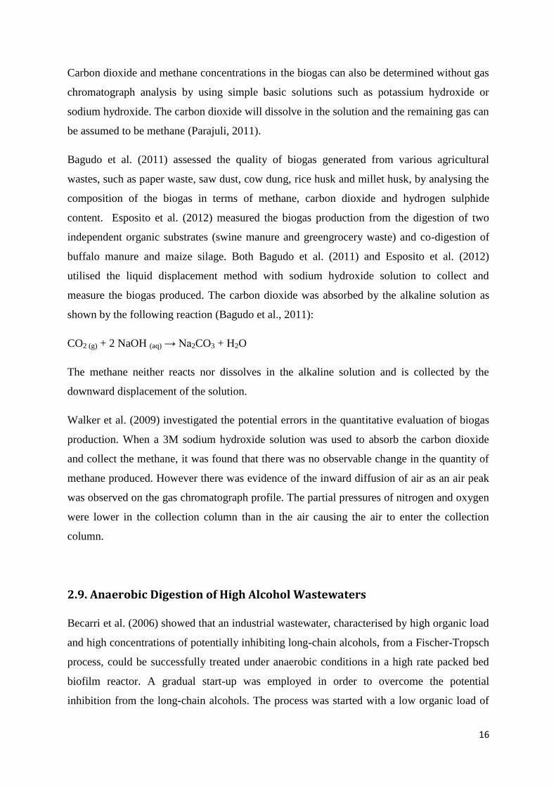
Carbon dioxide and methane concentrations in the biogas can also be determined without gas

chromatograph analysis by using simple basic solutions such as potassium hydroxide or

sodium hydroxide. The carbon dioxide will dissolve in the solution and the remaining gas can

be assumed to be methane (Parajuli, 2011).

Bagudo et al. (2011) assessed the quality of biogas generated from various agricultural

wastes, such as paper waste, saw dust, cow dung, rice husk and millet husk, by analysing the

composition of the biogas in terms of methane, carbon dioxide and hydrogen sulphide

content. Esposito et al. (2012) measured the biogas production from the digestion of two

independent organic substrates (swine manure and greengrocery waste) and co-digestion of

buffalo manure and maize silage. Both Bagudo et al. (2011) and Esposito et al. (2012)

utilised the liquid displacement method with sodium hydroxide solution to collect and

measure the biogas produced. The carbon dioxide was absorbed by the alkaline solution as

shown by the following reaction (Bagudo et al., 2011):

CO2 (g) + 2 NaOH (aq) → Na2CO3 + H2O

The methane neither reacts nor dissolves in the alkaline solution and is collected by the

downward displacement of the solution.

Walker et al. (2009) investigated the potential errors in the quantitative evaluation of biogas

production. When a 3M sodium hydroxide solution was used to absorb the carbon dioxide

and collect the methane, it was found that there was no observable change in the quantity of

methane produced. However there was evidence of the inward diffusion of air as an air peak

was observed on the gas chromatograph profile. The partial pressures of nitrogen and oxygen

were lower in the collection column than in the air causing the air to enter the collection

column.

2.9. Anaerobic Digestion of High Alcohol Wastewaters

Becarri et al. (2006) showed that an industrial wastewater, characterised by high organic load

and high concentrations of potentially inhibiting long-chain alcohols, from a Fischer-Tropsch

process, could be successfully treated under anaerobic conditions in a high rate packed bed

biofilm reactor. A gradual start-up was employed in order to overcome the potential

inhibition from the long-chain alcohols. The process was started with a low organic load of

17

3.4 g COD/ℓ/day and a modified synthetic wastewater with less or no long-chain alcohols.

The organic load and the concentration of the long-chain alcohols were then increased and

the COD removal, methane production and effluent concentration were monitored. It was

found that the reactor could be operated up to an organic load of 20 g COD/ℓ/day with no

loss of performance. A 96% COD removal and full conversion of the removed COD to

methane was achieved. The effluent contained only acetic and propionic acid that were easily

removed under aerobic conditions.

2.10. Anaerobic Digestion of High Phenolic Wastewaters and Phenolic

Compounds

Anaerobic digester upsets and failures may be caused by a wide range of inhibitory

substances which may be present in the wastewater in significant concentrations. Phenols are

among those substances that are known to inhibit anaerobic processes (Chen et al., 2007).

Kayembe et al. (2013) evaluated the inhibitory effects of phenolic monomers on

methanogenesis in anaerobic digestion. The effect of the number of hydroxyl groups in the

aromatic structure on the inhibition of methane production by acetoclastic methanogens was

also assessed. A serum bottle assay with a liquid displacement method to collect the biogas

was used to observe the methane production and therefore the specific methanogenic activity.

The biomass used was digested pig manure which had not been previously acclimated to any

aromatic compounds. The substrate was composed of acetic acid. Naturally occurring

phenolic compounds including phenol, resorcinol, hydroquinone and pyrogallol were used as

the potentially inhibitory aromatic compounds and benzene was used as the reference

aromatic compound. The inhibitory concentrations of benzene varied from 0 to 750 mg/ℓ.

The inhibitory concentrations of phenol and resorcinol varied from 0 to 4500 mg/ℓ. The

inhibitory concentrations of hydroquinone and pyrogallol varied from 0 to 10000 mg/ℓ. All of

the concentrations of the aromatic compounds tested were observed to have an inhibitory

effect on the specific acetoclastic methanogenic activity ranging from 0 – 100% inhibition.

The concentrations of benzene, phenol, resourcinol, hydroquinone and pyrogallol which

caused 50% inhibition of the methanogenic activity were 209 ± 6.32, 1249 ± 29.59,

1725 ± 5.27, 2745 ± 97.8 and 3173 ± 91.02 mg/ℓ, respectively. It was also found that as the

number of hydroxyl groups on the aromatic compounds increased, the phenolic monomers

18

toxicity decreased. Therefore the toxicity of the phenolic monomers increases in the

following order: pyrogallol < hydroquinone < resorcinol < phenol < benzene.

Fang et al. (1997) studied the effect of phenol on the methanogenic activity of three types of

UASB granules, with different bacterial composition and microstructure, in batch tests. The

three types of biogranules selected for these tests were from three different UASB reactors

degrading acetate, propionate and benzoate individually. The batch tests were carried out in

157 mℓ serum vials placed in a 37 °C shaking water bath. The biogranules were added to the

vials together with 100 mℓ of feed solution containing substrate, which was the same as the

substrate used in the biogranule-cultivating reactors mentioned previously, nutrients,

vitamins, trace metals and various concentrations of phenol. The control units contained a

phenol-free solution. The concentrations of phenol that caused 50% inhibition of the

methanogenic activity were 1750, 1000 and 1700 mg/ℓ for acetate-, propionate- and

benzoate-degrading biogranules. The concentrations of phenol that caused 100% inhibition of

the methanogenic activity were 3950, 2000 and 2200 mg/ℓ for acetate-, propionate- and

benzoate-degrading biogranules. The specific methanogenic activities (SMA) were measured

over 7 days. The toxicities of phenol were indicated by a decrease of the SMA relative to the

control units. It was observed that the higher the phenol concentration, the greater the SMA

reduction and therefore the higher the inhibition of the overall methanogenic activity.

Donaldson et al. (1987) evaluated a fluidised-bed bioreactor process for biooxidation of coal

gasification wastewater. The wastewater used was obtained from METC (Blacksville Coal)

and the majority of the sulphides and ammonia were stripped from the water using a steam

stripper. The biomass used to start up the bioreactor was one that had been used in previous

work. The bioreactor was started up on dilute phenol, mineral salts media and a small amount

of METC water (10%). During the next 5 days, dilute phenol mixed with METC water was

added to the bioreactor, first batch-wise in increasing amounts and then, after 3 days, with a

dilute continuous feed. Once the bioreactor was operating in a stable manner, feed makeup

was done once or twice a week which consisted of 2 ℓ METC water, 2 ℓ process water,

10 - 20 mℓ mineral salts media and 10 - 20 g of pure phenol. After approximately 3 months

of operation the additional phenol was phased out. When the build-up of biomass caused the

level of the fluidised-bed to become excessive about one-third of the bed volume was

withdrawn. At higher concentrations of phenol (greater than 400 ppm of phenol) the growth

of the biomass was slightly slower. During the stable operation of the bioreactor, its

performance was monitored by analysing the phenol concentration of the feed and the

19

effluent wastewater streams. The phenol concentration was analysed using the

4-aminoantipyrine method and the gas chromatograph with Carbowax or cross-linked 5%

phenyl column. Volumetric phenol degradation rates were calculated from the phenol

concentrations at the inlet and outlet of the bioreactor, the liquid flow rate and the settled bed

volume. Values in the range of 20 mg phenol/ℓ bed.min were achievable under proper

operating conditions. The phenol concentration was typically reduced by 40 - 50% depending

on the residence time.

Stepan (2006) investigated the technical feasibility of using an anaerobic process for the

treatment of the Dakota Gasification Company (DGC) stripped gas liquor (SGL). The

wastewater contained phenols, catechols, acids and alcohols. The phenolics concentration of

the wastewater was 500 mg/ℓ. A sample of recycle sludge was obtained from an anaerobic

digester (source of methanogenic bacteria) and was placed in a heated, mixed, glass reactor

vessel for acclimation and biomass development. The SGL was added in increasing amounts

to the reactor. Difficulty was experienced in establishing a high-rate catechol-degrading

culture and the acclimation period was longer than expected. Three bioreactors were operated

to acclimatise the biomass to the components of SGL. The reactor fed with synthetic SGL

emphasising catechol showed good removals of the catechol. However, the reactors fed with

actual SGL were inhibited and catechol degradation was negligible. It was suggested that the

catechol may have undergone a polymerisation reaction instead of degrading and producing

methane. The bioreactor system operation was continued and the feed dilution was decreased

until the catechol degradation could be sustained without inhibition using full-strength SGL

as the influent. The reactor feed was 5.3 ℓ/day and the gas production ranged from

3 - 4 ℓ/day. There was an improvement in the catechol degradation. The catechol degraded

such that the gas produced was half of the calculated theoretical production if all of the

catechol had been degraded. It was concluded that catechol can be degraded under anaerobic

conditions under the right operating conditions.

2.11. Summary

Anaerobic digestion is an attractive method of degrading organic matter as it has several

advantages; it does not require energy to aerate the system and it converts organic matter to

methane gas which can be used as a source of energy. However factors such as temperature

and pH have to be monitored closely to prevent system upsets. The serum bottle test is a

20

simple and reproducible technique to evaluate the anaerobic biodegradability of organic

matter by monitoring the biogas production. There are different methods of collecting and

measuring the biogas produced. The collection of the biogas by the downward displacement

of a saturated acidified brine solution showed the lowest carbon dioxide solubility and the

composition of the biogas could be analysed using a gas chromatograph. However the

composition of the headspace biogas is easily altered by the solubility of analyte gases in the

liquid phase resulting in inaccurate results. The use of the downward displacement of a

sodium hydroxide solution eliminated the errors arising from gas chromatograph

measurements by absorbing the carbon dioxide from the biogas produced, collecting only the

methane.

There was no literature that provided direct information for designing a Fischer-Tropsch

reaction water and stripped gas liquor co-digestion scheme. Literature did not provide an

answer of whether the stripped gas liquor would inhibit Fischer-Tropsch reaction water

digestion and to what extent and whether all of the components in stripped gas liquor can be

degraded in an anaerobic digestion scheme with a sludge acclimated to Fischer-Tropsch

reaction water only. There was no information regarding the anaerobic digestion kinetics of

Sasol stripped gas liquor. However information about the anaerobic digestion of high alcohol

wastewaters, similar to Fischer-Tropsch reaction water, and the anaerobic digestion of high

phenolic wastewaters, similar to stripped gas liquor, independently, could be obtained.

Fischer-Tropsch reaction water, from the Synthol process, contains organic acids and alcohol.

The anaerobic digestion of high alcohol wastewaters, similar to Fischer-Tropsch reaction

water, was researched. Becarri et al. (2006) showed that wastewaters with a high

concentration of long-chain alcohols can be successfully anaerobically digested by employing

a gradual start-up to acclimate the sludge to the wastewater. Therefore it can be presumed

that the Fischer-Tropsch reaction water used in this project will be readily degradable on its

own, especially since the sludge was acclimated to the Fischer-Tropsch reaction water prior

to the start of this project.

Stripped gas liquor, from the Phenosolvan plant, contains organic acids, ammonia and

phenols. The results of anaerobic digestion of high phenolic wastewaters, such as stripped gas

liquor, obtained from literature were reviewed. Kayembe et al. (2013) and Fang et al. (1997)

observed that phenolic compounds tended to inhibit the specific methanogenic activity in the

test units in comparison to the control units when the sludge was not acclimated to the

21

phenolic compounds. Since the sludge used in this project was not acclimated to the phenolic

compounds in stripped gas liquor, it was postulated that these phenolic compounds may

inhibit the anaerobic digestion of Fischer-Tropsch reaction water when stripped gas liquor is

added to the batch reactor.

Donaldson et al. (1987) and Stepan (2006) showed that phenol and catechol in stripped gas

liquor can be degraded under anaerobic conditions if the sludge is acclimated to the stripped

gas liquor. However, acclimation of the sludge to the phenolic compounds in stripped gas

liquor is very difficult. Stepan (2006) found that high-rate catechol-degrading cultures take a

long period of time to establish and Donaldson et al. (1987) observed that biomass growth

was slower at higher concentrations of phenol. Since the sludge used in this project was not

acclimated to stripped gas liquor prior to the start of this project, it can be reasonably

assumed that the anaerobic consortium that evolves during treatment of only Fischer-Tropsch

reaction water is only able to execute a limited range of metabolic pathways, selecting for

those micro-organisms that can most effectively metabolise short-chain volatile acids and

alcohols as found in Fisher-Tropsch reaction water. Therefore the micro-organisms capable

of metabolizing higher molecular weight organic contaminants, such as phenolic compounds,

found in stripped gas liquor may be slower growing and it is possible that they will not

establish to a significant degree in a mixed system. Thus by introducing stripped gas liquor to

the Fischer-Tropsch reaction water digester, there is a risk that the phenolic compounds will

not be treated. The final effluent will therefore be contaminated by these components, with

implications for reuse and discharge.

This project will be investigating the influence of stripped gas liquor on Fischer-Tropsch

reaction water digestion, the extent of inhibition of Fischer-Tropsch reaction water digestion

by stripped gas liquor, if any, and whether the phenolic compounds in stripped gas liquor will

be degraded by the Fischer-Tropsch reaction water acclimated sludge.

22

CHAPTER 3

3. Experiment Design

In chapter 3, the hypotheses of the project, which were developed based on the literature

reviewed, are discussed, the research outcomes expected to be achieved by the project are

stated and an experiment design in order to achieve the outcomes is presented. The materials

used throughout the project and the methods used to sample these materials, determine the

characteristics of the materials and to analyse the results obtained from the serum bottle tests

were outlined. In section 3.4, the source of the materials that are used in the serum bottle tests

and how these materials are sampled and stored are explained. In section 3.5, the methods

used to analyse the physicochemical characteristics of the materials before the serum bottle

tests are started and after the tests, to see the changes caused by the degradation of the

materials, are described. The biogas produced by the serum bottle test consists of carbon

dioxide and methane and it is important to know what composition of the biogas methane is

in order to determine the extent of the degradation that occurred. The analysis of the

composition of the biogas is covered in section 3.7. In section 3.8, an explanation of how the

phenol concentration in the stripped gas liquor can be measured before and after the serum

bottle tests, to obtain an indication of whether the FTRW acclimated sludge is capable of

degrading the high molecular weight organics in stripped gas liquor, is given. In section 3.9

and 3.10, the interpretation of the data obtained is detailed.

3.1. Hypotheses

The first hypothesis is that the anaerobic sludge, which is acclimated to Fischer-Tropsch

reaction water only, will be inhibited by the higher molecular weight organics such as

phenols in stripped gas liquor.

23

The second hypothesis is that the Fischer-Tropsch reaction water acclimated sludge will not

be able to degrade the phenolics in stripped gas liquor.

3.2. Research Outcomes

In order to test the hypotheses the following will be determined:

The influence of stripped gas liquor on the specific methanogenic activity of

Fischer-Tropsch reaction water acclimated sludge

The fate of indicator compounds for potentially toxic higher molecular weight

organics in stripped gas liquor, such as phenols, in batch anaerobic co-digestion

experiments

3.3. Overview of Experiment Design

Since this project was only the first step of a broader project to investigate the feasibility of

Fischer-Tropsch reaction water and stripped gas liquor co-digestion, there was no previous

data to base this project’s experiments on. Also, there was no information about the

co-digestion of FTRW and SGL in literature. Therefore many experiments needed to be

conducted to determine what loading rates and ratios of FTRW to SGL would be viable.

Therefore a continuous process would not be economical to use since a continuous reactor

takes time to start up and reach consistent steady state production. Thus, the serum bottle test,

which is a batch process, was the technique used to measure the methanogenic activity of the

Fischer-Tropsch reaction water and stripped gas liquor digested with a FTRW-acclimated

sludge, under mesophilic conditions, since it is simple and inexpensive. Although the serum

bottle technique does not give direct measurements of continuous process kinetics, it can

generate the maximum methane production rate which gives a good indication of the

maximum acetate utilisation rate of the aceticlastic methanogens (Conklin et al., 2008) and

therefore an idea of how the process would behave in a continuous reactor.

A method was developed to successfully collect the biogas produced. The liquid

displacement method was used and three different barrier solutions, to prevent the dissolution

of the biogas in the displacement liquid were tested, that is, tap water, acidified brine solution

and an alkaline solution.

24

Different COD loads of the FTRW were tested to determine what the base experiment should

look like and a reference test was selected. The SGL was then added to the base experiment

and the specific methanogenic activities of the reference units and test units were compared

to investigate whether the SGL would cause any inhibitory effect on the anaerobic digestion

of FTRW. The concentration of the indicator compounds in SGL (such as phenol) was tested

at the beginning and end of the co-digestion experiments, using the colorimetric method and

gas chromatograph, to determine the fate of the high molecular weight organics in SGL.

3.4. Materials

3.4.1. Sludge

The sludge used in the experiments were obtained from an upflow anaerobic sludge blanket

(UASB) reactor which had been operated for 9 months prior to the start of this study, in the

Pollution Research Group laboratory. The sludge had been acclimatised to Fischer-Tropsch

reaction water. The reactor was constructed with a bottom inlet for the wastewater, which

passed through the bed and the sludge blanket. When the sludge was sampled, the sludge was

first pumped around for approximately 30 minutes to ensure even distribution of the granules.

If the sludge was only to be used 1 – 2 days after sampling, it was stored in the cool room at

4 °C. The sludge was then incubated in a 2 ℓ Schott bottle in the water bath 24 hours before

the serum bottle test to increase the temperature of the sludge to the required temperature of

35 °C. Otherwise the sludge was used directly after sampling.

3.4.2. Substrates

The substrates were the Fischer-Tropsch reaction water, to which the sludge was

acclimatised, and the stripped gas liquor, which was the test substrate for the anaerobic

co-digestion. Both the Fischer-Tropsch reaction water and the stripped gas liquor were

received directly from the Sasol plant. The substrates were stored in the cool room at 4 °C.

On the day that the substrate was to be used, it was removed from the cool room and allowed

to reach room temperature.

25

3.4.3. Nutrients

The nutrients required to supplement the micro-organisms were prepared as described by

Owen et al. (1979). The nutrients were a combination of trace nutrients, macro-nutrients and

vitamins. The nutrients are said to be necessary for optimal growth of the micro-organisms

which would affect the ability of the micro-organisms to degrade the substrate.

Table 3-1: Table showing the stock solutions for the preparation of the nutrients

(Owen et al., 1979)

Solution Compound Concentration (g/ℓ)

S1 Resazurin 1

S2 (NH4)2HPO4 26.7

S3 CaCl2.2H2O 16.7

NH4Cl 26.6

MgCl2.6H2O 120

KCl 86.7

MnCl2.4H2O 1.33

CoCl2.6H2O 2

H3BO3 0.38

CuCl2.2H2O 0.18

Na2MoO4.2H2O 0.17

ZnCl2 0.14

S4 FeCl2.4H2O 370

S5 Na2S.9H2O 500

S6 Biotin 0.002

Folic acid 0.002

Pyridoxine hydrochloride 0.01

Riboflavin 0.005

Thiamin 0.005

Nicotinic acid 0.005

Pantothenic acid 0.005

B12 0.0001

ρ-aminobenzoic acid 0.005

Thioctic 0.005

26

3.5. Physicochemical Characteristics of Substrates and Sludge

3.5.1. pH test

The pH of the Fischer-Tropsch reaction water, the stripped gas liquor and the mixed liquor

from the serum bottles were measured using the Hanna pH meter (HI 255 combined meter).

Since the serum bottle test was a batch test and there was no online system to measure the pH

continuously, extra bottles were set up for the inhibition tests with the same composition of

sludge and substrates as the test units. These extra bottles were then sacrificed before and

after the serum bottle tests, as well as at intervals during the experiment to measure the pH

during the experiment.

3.5.2. Alkalinity test

Alkalinity is the measure of the capacity of the water to neutralise a strong acid to keep the

pH stable (Snoeyink et al., 1980). The alkalinity of a sample is a function of the

concentrations of the hydroxyl, carbonate and bicarbonate ions present. The method used to

determine the alkalinity involved adding a standardised acid to the sample until a colour

change of the indicator was observed or a predetermined end point pH of 4.5 was reached.

The indicator used was a mixture of bromocresol green and methyl red. However, since the

SGL used had such a dark brown colour, it was difficult to observe a colour change therefore

the end point was detected using a pH meter. Fischer-Tropsch reaction water had no

alkalinity since the pH of FTRW was already below 4.5.

3.5.3. Solids test

The total solids can be measured by taking a known volume of the sample and evaporating

the water contained in the sample by placing it in an oven at 103 – 105 °C and drying to a

constant weight. The residue remaining is the total solids which is comprised of suspended

solids and dissolved solids. Suspended solids are those solids that do not pass through a glass

microfiber filter paper (1 μm, 47 mm). After filtration the filter paper with the wet solids are

placed into the oven at a temperature of 103 – 105 °C for 30 minutes. The mass of solid

residue on the filter paper after drying is the total suspended solids. The dissolved solids are

the components, such as salts, in the sample filtrate that exist in the dissolved form but

27

precipitate when the sample is dried. The fixed solids can be determined by taking the

suspended solids and igniting it to a constant weight by placing it in a furnace at 550 °C for

1 hour. The volatile solids are the weight lost during ignition, while the fixed solids are the

mass remaining on the filter paper after ignition. These tests were performed on the substrates

(FTRW and SGL) and the sludge before any experiments were started.

3.5.4. Chemical oxygen demand test

The chemical oxygen demand (COD) is the amount of oxygen necessary to oxidise any

oxidisable material in a sample to water, carbon dioxide and ammonia. Chemical oxygen

demand is a conserved property, as the COD of a sample before anaerobic digestion is equal

to the sum of the COD of the substrate left and the COD removed and can be used to

determine the extent of the biodegradation of the substrate. In anaerobic digestion, COD is

only removed from the mixed liquor by conversion to gaseous methane, which escapes with

the biogas. Therefore measurement of the methane produced can be used to estimate the

COD removed from the mixed liquor by anaerobic digestion and hence the extent of

biodegradation of the substrate.

The oxygen demand can also be estimated by conducting a test using a chemical oxidising

agent. The COD is given as the amount of oxygen from the chemical oxidising agent used to

break down the organic compounds in a particular volume of sample under hot, acidic

conditions. The test is relatively quick and the results are reproducible. The most common

oxidizing agents used are potassium dichromate or potassium permanganate (Wiseman,

1978). In this study, the COD of the substrates and sludge were measured before the

experiments. Extra bottles were set up for the inhibition tests with the same composition of

sludge and substrates as the test units and these were sacrificed before, during and after the

experiment to measure the COD of the mixed liquor in the serum bottles. The samples were

digested for 2 hours in an ETHOS One microwave using the closed reflux method. The

program was set to ramp the temperature to 150 °C in 15 minutes, digest the sample at

150 °C for 30 minutes and then cool for 1 hour to 50 °C. The COD was then determined by

back titration of the oxidising agent when all the COD of the sample has been used up.

28

3.6. Serum Bottle Test

Figure 3.1: Diagram of a serum bottle, its components and contents

In a serum bottle test, the anaerobic sludge is placed in the vial together with the substrate to

degrade and the nutrient and mineral solution to provide the necessary micronutrients, such as

trace metals, amino acids and so forth, if necessary. The serum bottle is then kept at a

constant temperature of about 35°C for between 7 to 30 days using a water bath. As the

substrate is degraded, biogas is produced which consists of carbon dioxide and methane

(Owen et al., 1978). The biogas is then collected using a liquid displacement method where

the barrier solution could be either tap water, acidified brine solution or an alkaline solution.

This liquid displacement method generates biogas production activity as a function of time.

From this, the biogas production activity as a function of substrate concentration can be

inferred. The collection of the biogas produced is described in detail in Chapter 4, Method

Development.

3.7. Gas Composition Measurement

Since the biogas collected using the water displacement method and the acidified brine

solution method contained both methane and carbon dioxide, the biogas had to be analysed to

determine the percentage composition of each component. The Shimadzu gas chromatograph

with the GC Real Time Analysis programme was used for this purpose. The column used was

the Carboxen capillary column with an internal diameter of 2.1 mm and a length of 1.5 m,

29

which is suitable for the analyses of light hydrocarbons. A gas tight syringe was used to make

the injections manually with an injection port temperature of 25 °C. The volume of the gas

injected ranged from 0.1 to 0.4 mℓ. Helium was used as the carrier gas with a flow rate of

25 mℓ/min and the oven was held at a temperature of 100 °C for 8 minutes. The type of

detector used was a thermal conductivity detector (TCD) at a temperature of 25 °C. The gas

composition had to be measured as often as possible to obtain a reliable representation of

how the gas compositions were changing as the anaerobic digestion took place. However

since there were 12 serum bottles and triplicate readings were required for each bottle it was

not possible to measure the gas composition more than once a day with the manual injection

system available.

3.8. Phenol Measurement

One of the components in SGL that may inhibit biological activity is phenol. Although

phenol is not the only inhibitor, it was used as an indicator compound to determine the fate of

high molecular weight organics in SGL. Therefore it was important to measure the phenol

concentration (mg/ℓ) before and after anaerobic digestion to determine if the phenol could be

degraded by the FTRW acclimatised sludge and, if so, to what extent. There were two

methods whereby the phenol concentration could be determined, namely, the colorimetric

method and the gas chromatography. The colorimetric method was used to quantify all

phenolic compounds in a sample, while the GC was used for qualitative assessment of

phenolic compounds in the sample.

3.8.1. Colorimetric method

The first method used for the determination of the presence of phenols in the wastewater is

the colorimetric method. It is based on the reaction, observed by Emerson (1943), whereby

4-aminoantipyrine reacts with phenol forming an intensely red or purple coloured compound

in the presence of oxidising agents provided that the pH is high enough. The absorbance of

light of the solution at a given wavelength is measured using a spectrophotometer.

The bonding of the 4-aminoantipyrine with the phenol takes place in the para-position which

is opposite the OH group in the phenol. Therefore for the reaction to be possible the

30

para-position must either be free or occupied by a halogen, carboxyl, sulphonic acid,

hydroxyl or methyl group which is expelled to accommodate the 4-aminoantipyrine

(Emerson, 1943). Figure 3.2 below shows how 4-aminoantipyrine and phenol bond:

Figure 3.2: The reaction of 4-aminoantipyrine with phenol (Emerson, 1943)

If the pH is below 8, the 4-aminoantipyrine is instead oxidised to form the compound

antipyrine red (Ochynski, 1960). Therefore Gottlieb and Marsh (1946) suggest that a pH

range of 10.4 – 10.6 be used. Even a slight change in the pH may affect the intensity and the

stability of the colours produced. However it is very difficult to obtain the exact pH required

since the pH of the solution is usually analysed and accordingly adjusted before the addition

of the reagents which cause a drop in the pH value. A way to decrease the pH drop is to add

ammonium chloride which provides some buffering action and therefore stabilises the pH

(Dannis, 1951). The buffer solution used in the colorimetric analyses for this project was

made up of ammonium chloride and ammonium hydroxide.

The temperature is also a factor which affects the colour formation. To limit the effect that

the temperature has on the results, the samples should be analysed quickly (Ettinger, 1951). If

the samples are cloudy, intensely coloured or contain interfering compounds such as

sulphites, metallic ions, aromatic amines or quinones, distillation may be advisable before

any of the reagents are added. The distillation is done in a Pyrex all-glass distillation

apparatus after addition of copper sulphate and adjustment with phosphoric acid to

approximately pH 4 (Dannis, 1951). The phenolic compounds are separated out and the

distillate is analysed using the colorimetric method. The samples used in this project were

only slightly coloured therefore there was no need for distillation before the colorimetric

analysis.

31

The oxidising agent used was potassium ferricyanide because it allows rapid colour

formation, keeps the colour stable and has good sensitivity (Martin, 1949).

4-Aminoantipyrine is a good reagent due to the fact that it does not react with just the

alkaline oxidising agents alone to form coloured products, unlike p-aminophenol and

p-diamines which do (Emerson, 1943).

The absorbance was measured using a spectrophotometer at a wavelength of 510 nm. The

method used to determine the concentration of the samples was the standard addition method.

The standard addition method involved adding the buffer solution, aminoantipyrine solution,

potassium ferricyanide as well as a standard volume of sample (10 mℓ) to varying

concentrations of phenol. The absorbance was then plotted against the concentration and

extrapolated to the x-axis to obtain the phenol concentration in the sample (refer to

Appendix E4. Phenol measurement)

3.8.2. Gas chromatography

The Shimadzu gas chromatograph with the GC Solution programme was used to analyse the

effluent from the serum bottles for the presence of phenols. The column used was the

ZB-WAXplus column with an internal diameter of 0.25 mm and a length of 30 m, which is

suitable for the analyses of phenols. An automatic sample injector was used to make the

injections with an injection port temperature of 220 °C. The volume of the sample injected

was 1 μℓ. Helium was used as the carrier gas with a constant flow rate of 0.23 mℓ/min. The

oven temperature was programmed to ramp from 60 °C to 240 °C at a rate of 20 °C/min. The

oven temperature was then held at 240 °C for 6 minutes. Hydrogen was used to ignite the

flame ionisation detector (FID).

3.9. Data Interpretation

3.9.1. Cumulative volume

The cumulative volume of biogas can be plotted against the time of the test for the control

units (blanks), which contains only sludge and nutrients, the reference units, which contain

sludge, nutrients and Fischer-Tropsch reaction water and the test units, which contain sludge,

nutrients, Fischer-Tropsch reaction water and stripped gas liquor.

32

The purpose of the blank is to provide a measure of the endogenous biogas production rate. It

is assumed that the endogenous rate is due to cell death and decay, which occurs at the same

rate in the test units as in the blanks. The net volume of biogas can be plotted against time,

which can be calculated by subtracting the volume of methane measured from the blanks

from the volume of biogas measured from the test units. This gives the biogas generated by

the substrate only by eliminating the endogenous biogas production.

Figure 3.3: Representation of A) cumulative biogas volume vs time graphs of the control

(dashed line), reference unit and test unit and B) a net volume of biogas vs time graph

(solid line) (Source: Remigi et al., 2006)

There are various shapes (represented in Figure 3.3) that the cumulative biogas volume vs

time graph can take on depending on the biodegradability of the test material:

1. The test material is readily biodegradable

2. The test material is biodegradable after a lag phase

3. There is partial inhibition

4. There is complete inhibition

0

200

400

600

0 10 20 30 40Time

Vo

lum

e

Reference

Test unit

A

0

200

400

600

0 10 20 30 40Time

Vo

lum

e

B

33

Figure 3.4: Possible shapes of the graph of cumulative biogas volume vs time (Source:

Remigi et al., 2006)

3.9.2. Net methane volume

Equation 3-1

Where:

= Cumulative net volume of methane (mℓ) at time t

= Cumulative methane volume of test unit (mℓ) at time t

= Cumulative methane volume of blank (mℓ) at time t

3.9.3. Conversion of moles of methane to COD

The chemical oxygen demand (COD) is the amount of oxygen necessary to oxidise any

oxidisable material in a sample to water, carbon dioxide and ammonia. Therefore, to find the

COD of 1 mole of methane, the number of moles of oxygen needed to convert the methane to

carbon dioxide and water was determined:

Equation 3-2

Therefore 1 mole of methane = 2 moles COD

Since 1 mole of O2 = 1 mole COD = 32 g

1 mole of methane = 64 g COD

-150

-50

50

150

250

350

450

Time

Vo

lum

e

1 2 3

4

C

34

3.9.4. Conversion of COD to volume of methane

From above 1 mole of methane = 64 g COD

Using the ideal gas law, the volume of methane can be calculated

Equation 3-3

Where:

= Number of moles of methane (mol)

R = Universal gas constant = 8.314 (Pa.m3)/(mol.K)

= Temperature (K)

= Pressure (Pa)

Therefore 25 ℓ CH4 = 64 g COD

Giving 0.395 ℓ CH4 = 1 g COD (at atmospheric pressure and a reaction temperature of 35ºC)

3.9.5. Percentage COD recovery

In anaerobic digestion, COD is only removed from the mixed liquor by conversion to gaseous

methane, which escapes with the biogas. The percentage COD recovery shows what

percentage of the total COD added to the bottle was recovered as gaseous methane and thus

the extent of the biodegradation of the substrate.

Equation 3-4

(Remigi et al., 2006)

Where:

= The COD value of methane at the end of the experiment

= The initial COD value of substrate in the serum bottle

35

3.9.6. Specific methanogenic activity (SMA)

The specific methanogenic activity can be calculated as the amount of methane produced per

day per mass of volatile suspended solids, which is a surrogate measurement for the amount

of biomass. The specific methanogenic activity gives a good indication of the activity of the

biomass, and with this, a direct comparison between different experiments and different

substrates can be made.

Equation 3-5


Where:

= The net rate of methane production (mℓ/day)

= The biomass initially present in vial (gVSS)

The specific methanogenic activity of the sludge can then be plotted against time. These

curves also have different patterns depending on the effect the test material has on the activity

of the sludge (represented in Figure 3.5):

1. The test material is partially inhibitory but there is no lag phase or delay in the

methanogenic activity

2. The test material is partially inhibitory and there is a delay in the methanogenic

activity as the micro-organisms become acclimated to the test material

3. The test material is temporarily inhibitory and there is a lag phase before a specific

methanogenic activity, which is similar to that of the reference material, is observed

4. The test material is completely inhibitory and the sludge does not adapt to the test

material

36

Figure 3.5: Representation of B) specific methanogenic activity vs time graphs and C)

the possible shapes of the graph of specific methanogenic activity vs time (Source:

Remigi et al., 2006)

3.9.7. Inhibition

The inhibition effect can be calculated from:

Equation 3-6


Where:

= Specific methanogenic activity of the test unit (mℓ/gVSS.day)

= Specific methanogenic activity of the reference unit (mℓ/gVSS.day)

Therefore the inhibition is:

Equation 3-7


0

20

40

60

80

0 10 20 30 40Time

SM

A Reference

Test unit

B

0

20

40

60

80

0 10 20 30 40Time

SM

A

1

3

24

Reference

C

37

3.10. Statistical Methods

3.10.1. Confidence limits for a mean

The confidence interval is an indication of the reliability of the data. For a 95% confidence

interval, = 0.025 since the confidence level is defined as (1 – 2 ) for a two-tailed problem.

The confidence limits can be calculated from (Davies and Goldsmith, 1977):

⁄

√ Equation 3-8

Where:

= Mean value of measurements variable x

t = t-statistic for degrees of freedom at a confidence level of (1 – 2 ) for a two-tailed

problem

n = Number of observations

= Significance level

s = Estimated standard deviation of a population calculated from a sample

3.10.2. Difference between two means

In order to determine the confidence limits for the average difference between the means of

two independent data sets the following calculation can be used (Davies and Goldsmith,

1977):

√

Equation 3-9

Where:

and = The mean values of measurements variables and respectively

t = t-statistic for degrees of freedom at a confidence level of (1 – 2a) for a two-tailed

problem

= Number of degrees of freedom

and = Number of observations in data sets 1 and 2 respectively

= Significance level

38

and = Estimated standard deviation of data sets 1 and 2 respectively

The number of degrees of freedom, , can be calculated from:

[

]

[

]

Equation 3-10

Where:

3.10.3. Paired two sample t-test

The paired two sample t-test is a widely used statistical method to compare the means of

two data sets of paired samples. The paired t-test examines if the difference between the

means is significantly different from the hypothesised value of zero, = 0

(Park, 2009). Microsoft Excel was used to execute the t-test to compare the two sets of

data. The P value displayed in the table of results describes the probability that the

measured data would be obtained (assuming a normal distribution of measurement errors) if

the null hypothesis is supported. Therefore a value of P = 0.05 means that there is a 5%

probability that the calculated value between the measurement of the two means would have

been obtained if there was no significant difference between the two measurement

populations (Davies and Goldsmith, 1977).

39

CHAPTER 4

4. Method Development

The design of the method and the equipment used to attain the objectives of this research

project are extremely important as they directly affect the quality and reliability of the results.

In chapter 4, the details of the development of the method and equipment, from the water

displacement method (Section 4.1) through to the acidified brine solution method (Section

4.2) and finally to the alkaline solution method (Section 4.3) is given, providing results which

support the reasons for the changes made. The advantages and disadvantages of each method

are compared. In section 4.4, the reference test, which contains only sludge and

Fischer-Tropsch reaction water, is selected. This is to determine the reference activity when

the test material is not present. Different COD loads of FTRW were tested to determine

which gave the most reproducible results with different batches of sludge. Therefore there is

a known methane production to which the results from the co-digestion experiments can be

compared to determine whether the methanogenic activity is enhanced or inhibited by the

addition of the stripped gas liquor. In sections 4.4.1 and 4.4.2, the results obtained when COD

loads of 1, 1.5 and 2 g COD/ℓ of FTRW are used with different batches of sludge are

presented. The results are compared in Section 4.4.3 to determine the reproducibility when

different batches of sludge are used.

4.1. Water Displacement Method

The initial set-up consisted of twelve 250 mℓ serum bottles with screw-on caps, a water bath

and temperature regulator, a metal rack to place the serum bottles in, 24 droppers, 12 pipes of

the same length and a stand to attach the droppers to. The method used to collect the biogas

was a water displacement method. The droppers were arranged in pairs so that one dropper

acted as a gas collection dropper filled with water and the other dropper above it acted as an

40

overflow chamber to collect the displaced water. The biogas was collected by attaching one

end of a pipe to the serum bottle in which the anaerobic digestion was taking place and the

other end to the top of the gas collection dropper. As the biogas was produced it flowed

directly into the gas collection dropper and displaced the water with a volume equal to the

volume of gas produced. Therefore there was no need to vent the serum bottles so often. The

gas volume could be read directly off the graduations on the dropper. Since the total biogas,

which consists of methane and carbon dioxide, was collected in the gas collection dropper,

the gas composition had to be analysed in a Shimadzu 2010 gas chromatograph.


dropper arrangement for one of the bottles

35 °C

3

2

4

5

6

7

1

8

1 - Temperature regulator 2 - Water bath 3 - Metal bottle rack 4 - 250 ml Serum bottle 5 - Connecting pipes 6 - Gas collection dropper 7 - Overflow chamber 8 - Metal dropper stand

41

Figure 4.2: Photograph of the arrangement of the droppers with the bottom droppers

being the gas collection droppers and the droppers above being the overflow chambers

Figure 4.3: Photograph showing the attachment of the serum bottles in the water bath

to the gas collection droppers

42

Table 4-1: Table showing the concentration of the substrates and the type of gas

measurement used in the method development experiments

Experiment Type of gas

measurement

Sodium

acetate

(g COD/ℓ)

FTRW

(g COD/ℓ)

SGL

(g COD/ℓ)

Sludge Purpose of experiment

Trial run 1 Water

displacement

2.5 0 0 Brewery Proof of concept

Trial run 2 Water

displacement

2.5 0 0 Brewery Proof of concept

Set 1 Water

displacement

0 1.2, 1.5, 1.8 0 UASB 1 Selection of F:M ratio

Set 2 Acidified

brine solution

0 1.5 0 UASB 1 Test acidified brine

solution displacement

method

Set 3 Acidified

brine solution

0 5 0 UASB 1 Test necessity of

additional nutrient

supplementation

Set 4 Acidified

brine solution

0 1, 1.5, 2 0 UASB 2 Selection of F:M ratio

Set 5 Acidified

brine solution

& alkaline

solution

0 1 0 UASB 2 Comparison of acidified

brine solution method to

alkaline solution method

Set 6 Alkaline

solution

0 1, 1.5, 2 0 UASB 2 Selection of FTRW

concentration

Set 7 Alkaline

solution

0 1, 1.5, 2 0 UASB 2 Selection of FTRW

concentration

4.1.1. Proof of concept

In order to prove that this set-up works, two trial runs were carried out using brewery sludge

and acetate. A stock solution was made up using sodium acetate and distilled water such that

when 5 mℓ of the solution was added to each bottle it provided a concentration of

2.5 g COD/ℓ. The calculations for the preparation of the stock solution and the theoretical

amount of biogas that should be produced (approximately 436 mℓ) can be found in

Appendix C. Although the experiments were not run to completion (i.e. until the methane

production curve flattened out and there was no further production of methane) it can be seen

43

from Figure 4.4 and Figure 4.5 that the set-up works. The small error bars indicate that the

serum bottle experiment gives good, reproducible results.


(days) in trial run 1


(days) in trial run 2

0

50

100

150

200

250

0 0.5 1 1.5 2 2.5 3 3.5

Cu

mu

lati

ve n

et

bio

gas

pro

du

ctio

n (

mℓ

)

Time (days)

0

50

100

150

200

250

0 0.5 1 1.5 2 2.5 3 3.5 4

Cu

mu

lati

ve n

et

bio

gas

pro

du

ctio

n (

mℓ

)

Time (days)

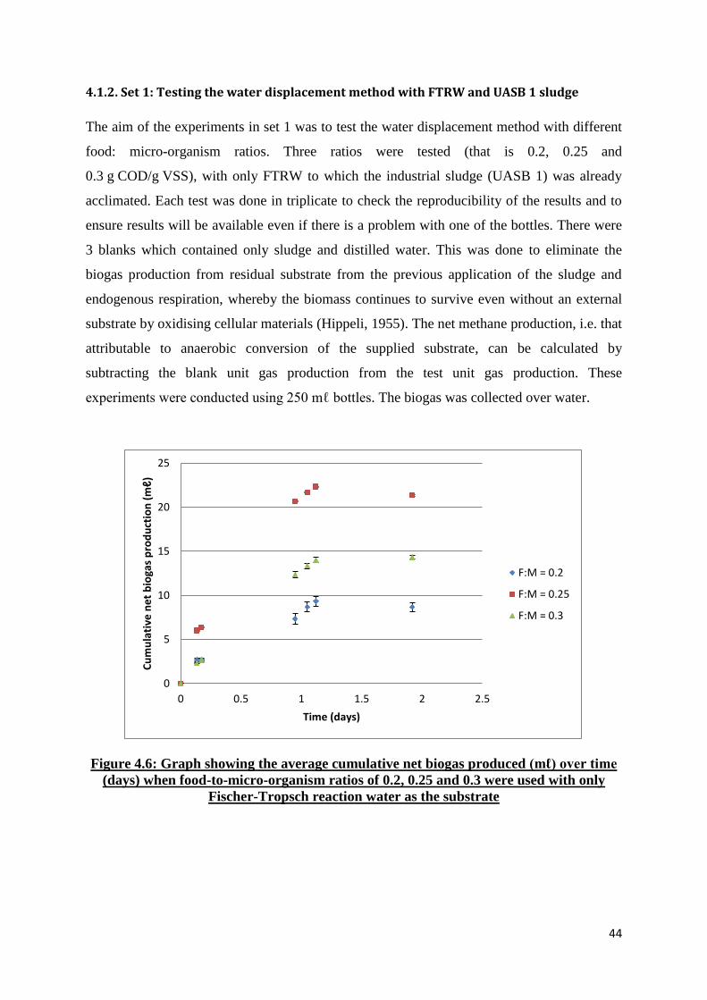
44

4.1.2. Set 1: Testing the water displacement method with FTRW and UASB 1 sludge

The aim of the experiments in set 1 was to test the water displacement method with different

food: micro-organism ratios. Three ratios were tested (that is 0.2, 0.25 and

0.3 g COD/g VSS), with only FTRW to which the industrial sludge (UASB 1) was already

acclimated. Each test was done in triplicate to check the reproducibility of the results and to

ensure results will be available even if there is a problem with one of the bottles. There were

3 blanks which contained only sludge and distilled water. This was done to eliminate the

biogas production from residual substrate from the previous application of the sludge and

endogenous respiration, whereby the biomass continues to survive even without an external

substrate by oxidising cellular materials (Hippeli, 1955). The net methane production, i.e. that

attributable to anaerobic conversion of the supplied substrate, can be calculated by

subtracting the blank unit gas production from the test unit gas production. These

experiments were conducted using 250 mℓ bottles. The biogas was collected over water.

Figure 4.6: Graph showing the average cumulative net biogas produced (mℓ) over time

(days) when food-to-micro-organism ratios of 0.2, 0.25 and 0.3 were used with only

Fischer-Tropsch reaction water as the substrate

0

5

10

15

20

25

0 0.5 1 1.5 2 2.5

Cu

mu

lati

ve n

et

bio

gas

pro

du

ctio

n (

mℓ

)

Time (days)

F:M = 0.2

F:M = 0.25

F:M = 0.3

45


(days) when food-to-micro-organism ratios of 0.2, 0.25 and 0.3 were used with only

Fischer-Tropsch reaction water as the substrate

It can be observed in Figure 4.6 that the average cumulative net biogas volume decreased

after 1.2 days instead of increasing as expected. This gave a negative specific biogas

production rate as shown in Figure 4.7. This decrease was reproducible in all 9 units that

were tested in this experiment. This may be due to the gaseous carbon dioxide of the biogas

which is produced being dissolved in or diffusing through the displacement liquid (Parajuli,

2011), in this case water.

4.2. Acidified Brine Solution Method

The acidified brine solution method is similar to the water displacement method. All of the

equipment and the components are identical. However the water in the gas collection dropper

is replaced with acidified brine solution to prevent the carbon dioxide collected in the dropper

from dissolving in the displacement liquid (Iyagba, 2009).

-1

0

1

2

3

4

5

6

0 0.5 1 1.5 2 2.5

Spe

cifi

c b

ioga

s p

rod

uct

ion

rat

e

(mℓ

/gV

SS.d

ay)

Time (days)

F:M = 0.2

F:M = 0.25

F:M = 0.3

46


UASB 1 sludge

From set 1 it was clear that the biogas could not be collected over water and that some sort of

barrier was needed to prevent the carbon dioxide from dissolving. According to Iyagba,

Mangibo and Mohammad (2009) an acidified brine solution could prevent the dissolution of

the biogas. Therefore this method was tested in set 2. A solution was added to the droppers

(which was prepared by adding sodium chloride to water until saturated and then adding a

few drops of sulphuric acid to acidify it). A food: micro-organism ratio of 0.25 g COD/g VSS

was used.


(days) with UASB 1 sludge, nutrients and Fischer-Tropsch reaction water as the

substrate

0

1

2

3

4

5

6

7

8

9

0 0.5 1 1.5 2 2.5

Cu

mu

lati

ve n

et

bio

gas

pro

du

ctio

n (

mℓ

)

Time (days)

47


(days) with UASB 1 sludge, nutrients and Fischer-Tropsch reaction water as the

substrate

Figure 4.8 shows a smoother curve than that observed in Figure 4.6. The specific biogas

production rate observed in Figure 4.9 remained positive throughout the experiment

indicating that the cumulative net biogas production in set 2 did not decrease during the

experiment. This suggests that the acidified brine solution lowered the solubility of the

carbon dioxide in the displacement liquid to a certain extent. Therefore this method of

collecting the gas was continued in the subsequent tests.

4.2.2. Set 3: Testing the necessity of additional nutrient supplementation

Set 3 was testing whether the use of additional nutrients in the serum bottles to supplement

the sludge was required. The preparation of the nutrients was presented in Section 3.4.3.

Nutrients). A food: micro-organism ratio of 0.25 g COD/g VSS was used with FTRW as the

only substrate and UASB 1 sludge. The biogas produced was collected using the acidified

brine solution displacement method.

0

0.5

1

1.5

2

2.5

3

3.5

4

4.5

0 0.5 1 1.5 2 2.5

Spe

cifi

c b

ioga

s p

rod

uct

ion

rat

e

(mℓ

/gV

SS.d

ay)

Time (days)

48

Figure 4.10: Graph showing the average cumulative net biogas production (mℓ) over

time (days) with UASB 1 sludge and Fischer-Tropsch reaction water as the substrate

Figure 4.11: Graph showing the specific biogas production rate (mℓ/gVSS.day) over

time (days) with UASB 1 sludge and Fischer-Tropsch reaction water as the substrate

The biogas production (Figure 4.10) and the specific biogas production rates (Figure 4.11)

in the bottles without additional nutrients and with additional nutrients were similar.

Therefore the use of additional nutrients to supplement the sludge was not necessary for

experiments carried out over a short time period and additional nutrients were not used in

0

2

4

6

8

10

12

14

16

0 1 2 3 4

Cu

mu

lati

ve n

et

bio

gas

pro

du

ctio

n (

mℓ

)

Time (days)

Without nutrients

With nutrients

-0.5

0

0.5

1

1.5

2

2.5

3

0 1 2 3 4

Spe

cifi

c b

ioga

s p

rod

uct

ion

rat

e

(mℓ

/gV

SS.d

ay)

Time (days)

Without nutrients

With nutrients

49

subsequent experiments. This may be due to the fact that the sludge was obtained from a

UASB reactor which was being fed nutrients frequently, including nitrogen supplementation.

In a batch test with relatively low growth requirement, the nutrients present in the UASB

sludge was sufficient for additional growth that occurred. In addition, some nutrients,

particularly reduced nitrogen are present in SGL. The fact that nutrients were not required for

the batch test does not negate the purpose of this research to use nitrogen in SGL to provide

nutrients for FTRW digestion. The batch serum bottle test with pre-conditioned sludge had

sufficient nutrients for the growth requirements for the duration of the test. However, in a

continuous system treating FTRW, the nutrients at the start of the continuous operation would

be depleted by growth and dilution. Therefore these results do not suggest that there is no

value in using SGL as a nitrogen source for the digestion of FTRW.


UASB 2 sludge

From the low volume of biogas collected in the previous experiments it was questionable

whether the UASB 1 sludge was still active. Therefore the aim of the experiments in set 4

was to test the UASB 2 sludge with different food: micro-organism ratios. Three

food: micro-organism ratios were tested (that is 0.03, 0.05, 0.07 g COD/g VSS), to which the

sludge from UASB 2 (mixture of brewery and municipal sludge) is already acclimated. The

food: micro-organism ratios corresponded to COD values of 1, 1.5 and 2 g COD/ℓ

respectively. Each test was done in triplicate to check the reproducibility of the results and to

ensure results were available even if there is a problem with one of the bottles. There were 3

blanks which contained only sludge and water. The biogas was collected over an acidified

brine solution.

50


time (days) with UASB 2 sludge and different concentrations of FTRW


time (days) with UASB 2 sludge and different concentrations of FTRW

The total volume of biogas produced using UASB 2 sludge in set 4 was much higher than

that produced by UASB 1 sludge in set 2 even with food: micro-organism ratios which are

much lower than those used in the previous experiments. Therefore the use of UASB 2 sludge

was continued in subsequent tests. Figure 4.12 shows the cumulative biogas volume

0

10

20

30

40

50

60

70

80

90

0 1 2 3 4 5 6

Cu

mu

lati

ve n

et

bio

gas

pro

du

ctio

n (

mℓ

)

Time (days)

1 g COD/l

1.5 g COD/l

2 g COD/l

-1

0

1

2

3

4

5

6

0 1 2 3 4 5 6

Spe

cifi

c b

ioga

s p

rod

uct

ion

rat

e

(mℓ

/gV

SS.d

ay)

Time (days)

1 gCOD/l

1.5 gCOD/l

2 gCOD/l

51

produced. There is no evidence of inhibition at high substrate loading which is indicated by

the fact that the cumulative volume of biogas produced at the end of the experiment was in

proportion to the initial organic loading. Figure 4.13 shows the specific biogas production

rate which also appears to be in proportion to the initial loading rate. Therefore the growth

rate was not saturated with respect to the substrate concentration in these experiments. The

theoretical volume of biogas that could have been produced with 1 g COD/ℓ of FTRW was

calculated to be about 165 mℓ (assuming that the only non-dissolvable gas was methane with

a composition of 60% with regards to the total volume of biogas produced). However this

set-up produced less than half of what was expected. This low gas production and the

decrease of the cumulative biogas already produced can be explained by the fact that as more

gas is produced in the serum bottle, the higher the concentration of carbon dioxide in the

headspace which then affects the concentration of carbon dioxide in the liquid phase and

consequently the pH. When the pH increases it causes carbon dioxide in the headspace to

dissolve into the liquid phase causing the noticeable decrease in the cumulative volume

(Parajuli, 2011). This would not be an issue if the methane composition from the gas analysis

using the gas chromatograph were reliable since the methane remains in the gas phase.

However technical problems with the GC analysis prevented gas composition data being

collected for these experiments. Therefore a method to collect the gas and absorb the carbon

dioxide, leaving only methane, was investigated, with the hope of eliminating the uncertainty

caused by the carbon dioxide dynamics.

4.2.4. Advantages and disadvantages of the acidified brine solution displacement method

Advantages Disadvantages

Theoretically gives total biogas

produced

With GC analysis can get

more information about CH4 and CO2

composition

Can observe independent changes in

specific methane production rate and

specific total gas production rate

CO2 is partially retained in solution

making gas production data difficult

to interpret

GC analysis wasn’t giving reliable

results at the time

When equilibrating, air enters the

bottle and affects the CO2 dynamics

even further

52

4.3. Alkaline Solution Method

This set-up consists of twelve 250 mℓ serum bottles with screw-on caps, a water bath and

temperature regulator, a metal rack to place the serum bottles in, twelve more serum bottles

filled with an alkaline solution, twelve 100 mℓ plastic cylinders, twelve pipes of the same

length and a stand to attach the serum bottles filled with the alkaline solution and the plastic

cylinders to. The method used to collect the biogas involves bubbling the biogas through the

alkaline solution. The alkaline solution absorbs the carbon dioxide from the biogas leaving

only methane which is collected above the alkaline solution. The volume of alkaline solution

displaced is equal to the volume of methane collected. The displaced alkaline solution is

collected in the plastic cylinder below the serum bottle filled with the alkaline solution and

the volume can be read directly off the graduations on the plastic cylinder (Esposito et al.,

2012). If the solution becomes saturated with carbon dioxide the thymol blue indicator will

change the solution from blue to a purple-orange colour.


dropper arrangement for one of the bottles

35

°C

1 2

3

4

5

6

8

7

1 - Temperature regulator 2 - Water bath 3 - Metal bottle rack 4 - 250 ml Serum bottle 5 - Connecting pipe 6 - Stand 7 - Gas collection bottle with NaOH solution 8 - Solution collection cylinder

53

Figure 4.15: Photograph of the arrangement of the inverted bottles, filled with sodium

hydroxide solution, above the plastic cylinders

Figure 4.16: Photograph of showing the attachment of the serum bottles in the water

bath to the inverted bottles filled with sodium hydroxide solution

54

4.3.1. Set 5: Comparison of the acidified brine solution method to the alkaline solution

method

In set 5 the acidified brine solution and the alkaline solution gas collection methods were

compared. Six bottles were set up with the acidified brine solution displacement method. The

other six bottles were set up with the alkaline solution method. The alkaline solution was

prepared by adding 50 g/ℓ of sodium hydroxide to distilled water and a pinch of thymol blue

indicator. The tests were done in triplicate using both methods. A food: micro-organism ratio

of 0.03 g COD/g VSS was used (which corresponded to an FTRW concentration of

1 g COD/ℓ) with the UASB 2 sludge.


time (days) with UASB 2 sludge and 1 g COD/ℓ of FTRW using the acidified brine

solution method

-20

0

20

40

60

80

100

0 2 4 6 8 10 12 14Cu

mu

lati

ve n

et

bio

gas

pro

du

ctio

n

(mℓ

)

Time (days)

55


time (days) with UASB 2 sludge and 1 g COD/ℓ of FTRW using the acidified brine

solution method

Figure 4.19: Graph showing the average cumulative net methaneproduction (mℓ) over

time (days) with UASB 2 sludge and 1 g COD/ℓ of FTRW using the alkaline solution

method

-0.5

0

0.5

1

1.5

2

2.5

3

0 2 4 6 8 10 12 14

Spe

cifi

c b

ioga

s p

rod

uct

ion

rat

e

(mℓ

/gV

SS.d

ay)

Time (days)

0

10

20

30

40

50

60

70

80

90

100

0 2 4 6 8 10 12 14 16

Cu

mu

lati

ve n

et

me

than

e p

rod

uct

ion

(m

ℓ)

Time (days)

56


(days) with UASB 2 sludge and 1 g COD/ℓ of FTRW using the alkaline solution method

Figure 4.17 shows the total biogas produced and collected using the acidified brine solution

method for 1 g COD/ℓ of FTRW. Figure 4.19 shows the methane produced and collected

using the alkaline solution method for 1 g COD/ℓ of FTRW. The theoretical volume of

methane that could have been produced with 1 g COD/ℓ of FTRW is approximately 99 mℓ

(assuming that methane is the only non-dissolvable gas produced). The theoretical volume of

total biogas that could be produced with 1 g COD/ℓ of FTRW is approximately 165 mℓ

(assuming that the composition of methane with regards to the total volume of biogas

produced is 60%). Since Figure 4.17 shows the results for the acidified brine solution method

which collects the total biogas produced, the cumulative volume should be much higher than

(almost double) that shown in Figure 4.19, which is only the methane production. However,

Figure 4.17 shows that only 80 mℓ of biogas was produced instead of the theoretical volume

of biogas of 165 mℓ. This indicates that at least half of the biogas produced is being retained

in the solution in the serum bottle giving inaccurate results. Figure 4.19 shows that the

volume of methane collected using the alkaline solution method was 90 mℓ which is very

close to the theoretical volume of methane of 99 mℓ. The initial specific methanogenic

activity of the sludge observed in Figure 4.20 when using the alkaline solution method of gas

collection was also higher than the initial specific biogas production rate observed in Figure

4.18 when the acidified brine solution method was used. Therefore the alkaline solution

method is a much more reliable means of collecting the gas produced.

-0.5

0

0.5

1

1.5

2

2.5

3

0 2 4 6 8 10 12 14 16

Spe

cifi

c m

eth

ano

gen

ic a

ctiv

ity

(mℓ

/gV

SS.d

ay)

Time (days)

57

4.3.2. Advantages and disadvantages of the alkaline solution method

Advantages Disadvantages

Gives methane production only

Eliminates uncertainties arising from

the CO2 dynamics

No need for GC analysis

Direct measurement of specific

methanogenic activity

Gives no indication of the activity of

the acidogenic micro-organisms

4.4. Reference Test

4.4.1. Set 6

In set 6 three concentrations of FTRW were tested (that is 1, 1.5 and 2 g COD/ℓ), to which

the sludge from UASB 2 was already acclimated. The respective food: micro-organism ratios

were 0.03, 0.05 and 0.07 g COD/g VSS. The biogas was bubbled through an alkaline solution

so that the carbon dioxide was absorbed leaving only the methane produced. The methane

was collected above the alkaline solution and displaced a volume of the solution equal to the

volume of methane produced. The solution was collected in a cylinder from which the

volume could be read directly. Each test was done in triplicate to check the reproducibility of

the results and to ensure results were available even if there was a problem with one of the

bottles.

58

Figure 4.21: Graph showing the average cumulative net methane production (mℓ) over

time (days) with UASB 2 sludge and 1, 1.5 and 2 g COD/ℓ of FTRW


(days) with UASB 2 sludge and 1, 1.5 and 2 g COD/ℓ of FTRW

Figure 4.21 shows the net methane production for set 6 where 1, 1.5 and 2 g COD/ℓ of

FTRW was tested. The small error bars in Figure 4.21 indicate that the three replicates of

each FTRW concentration showed identical behaviour. From Figure 4.21 it can be observed

that the bottles with the higher concentration of organics (higher COD values of FTRW)

produced larger volumes of methane. Figure 4.22 shows the specific methanogenic activity

0

10

20

30

40

50

60

70

80

90

0 2 4 6 8

Cu

mu

lati

ve n

et

me

than

e p

rod

uct

ion

(m

ℓ)

Time (days)

1 g COD/l

1.5 g COD/l

2 g COD/l

0

1

2

3

4

5

6

7

0 2 4 6 8

Spe

cifi

c m

eth

ano

gen

ic a

ctiv

ity

(mℓ

/gV

SS.d

ay)

Time (days)

1 gCOD/l

1.5 gCOD/l

2 gCOD/l

59

for set 6 experiments. A paired two sample t-test indicated that the SMA for the 1 g COD/ℓ

FTRW test unit was significantly lower than for the 1.5 g COD/ℓ FTRW test unit test at a

95% confidence level (P = 0.038). A paired two sample t-test also indicated that the SMA for

the 1.5 g COD/ℓFTRW test unit was significantly lower than for the 2 g COD/ℓ FTRW test

unit test at a 95% confidence level (P < 0.01). This suggests that an increase in the

concentration of FTRW tested with this batch of sludge resulted in an increase in the

methanogenic activity as expected and that there was no inhibition of this batch of sludge up

to 2 g COD/ℓ of the FTRW, to which the sludge was acclimated.

4.4.2. Set 7

The aim of the experiments in set 7 was to determine which food: micro-organism ratio was

the most reliable by comparing the results obtained from this experiment with the results

obtained from other batches of sludge tested with the same COD values of FTRW. The same

three concentrations of FTRW were tested (that is 1, 1.5 and 2 g COD/ℓ), to which the sludge

from UASB 2 (mixture of brewery and municipal sludge) was already acclimated. The

respective food: micro-organism ratios were 0.03, 0.05 and 0.07 g COD/g VSS. Each test was

done in triplicate to check the reproducibility of the results and to ensure results were

available even if there was a problem with one of the bottles. There were 3 blanks which

contained only sludge and water.

Figure 4.23: Graph showing the average cumulative net methane production (mℓ) over

time (days) with UASB 2 sludge and 1, 1.5 and 2 g COD/ℓ of FTRW

0

10

20

30

40

50

60

0 2 4 6 8

Cu

mu

lati

ve n

et

me

than

e p

rod

uct

ion

(m

ℓ)

Time (days)

1 g COD/l

1.5 g COD/l

2 g COD/l

60


(days) with UASB 2 sludge and 1, 1.5 and 2 g COD/ℓ of FTRW

Figure 4.23 shows the net methane production for set 7 where 1, 1.5 and 2 g COD/ℓ of

FTRW was tested. The small error bars in Figure 4.23 indicate that the three replicates of

each FTRW concentration showed identical behaviour. From Figure 4.23 it can be observed

that the bottles with the higher concentration of organics (higher COD values of FTRW) did

not produce larger volumes of methane as expected. At the beginning of the experiment (over

the first 4 days) the methane volumes produced by the 1.5 and 2 g COD/ℓ FTRW test units

were higher than the 1 g COD/ℓ test units. However after 4 days, the bottles with the lower

concentration of organics, the 1 g COD/ℓ test units, produced more methane than those

bottles with the higher concentration of organics (1.5 and 2 g COD/ℓ test units). Figure 4.24

shows the specific methanogenic activity for set 7 experiments. A paired two sample t-test

indicated that the SMA for the 1 g COD/ℓ FTRW test unit was not significantly different

from the 1.5 g COD/ℓ FTRW test unit test at a 95% confidence level. A paired two sample

t-test indicated that the SMA for the 1 g COD/ℓ FTRW test unit was significantly lower than

for the 2 g COD/ℓ FTRW test unit test at a 95% confidence level over the first 2 days

(P = 0.013). A paired two sample t-test over the rest of the data (after 2 days) indicated that

the SMA for the 2 g COD/ℓ FTRW test unit was significantly lower than for the 1 g COD/ℓ

FTRW test unit test at a 95% confidence level (P < 0.001). This suggests that an increase in

the concentration of FTRW tested with this batch of sludge did not result in an increase in the

-0.2

0

0.2

0.4

0.6

0.8

1

1.2

1.4

1.6

1.8

0 2 4 6 8

Spe

cifi

c m

eth

ano

gen

ic a

ctiv

ity

(mℓ

/gV

SS.d

ay)

Time (days)

1 gCOD/l

1.5 gCOD/l

2 gCOD/l

61

methanogenic activity as expected and that there may be inhibition of this batch of sludge at

2 g COD/ℓ of the FTRW.

4.4.3. Comparing results from different batches of sludge

The cumulative net methane volume and the specific methanogenic activity of each FTRW

concentration was compared for set 6 and set 7.

Figure 4.25: Graph showing the cumulative net methane production (mℓ) over time

(days) from different batches of sludge when 1 g COD/ℓ FTRW is used

0

10

20

30

40

50

60

70

0 2 4 6 8

Cu

mu

lati

ve n

et

me

than

e p

rod

uct

ion

(m

ℓ)

Time (days)

Set 6

Set 6

Set 7

Set 7

62




(days) from different batches of sludge when 1.5 g COD/ℓ FTRW is used

-0.5

0

0.5

1

1.5

2

2.5

3

0 2 4 6 8

Spe

cifi

c m

eth

ano

gen

ic a

ctiv

ity

(mℓ

/gV

SS.d

ay)

Time (days)

Set 6

Set 6

Set 7

Set 7

0

10

20

30

40

50

60

70

0 2 4 6 8

Cu

mu

lati

ve n

et

me

than

e p

rod

uct

ion

(m

ℓ)

Time (days)

Set 6

Set 6

Set 6

Set 7

63


(days) from different batches of sludge when 1.5 g COD/ℓ FTRW is used



0

0.5

1

1.5

2

2.5

3

3.5

4

4.5

5

0 2 4 6 8

Spe

cifi

c m

eth

ano

gen

ic a

ctiv

ity

(mℓ

/gV

SS.d

ay)

Time (days)

Set 6

Set 6

Set 6

Set 7

0

10

20

30

40

50

60

70

80

90

0 2 4 6 8

Cu

mu

lati

ve n

et

me

than

e p

rod

uct

ion

(m

ℓ)

Time (days)

Set 6

Set 6

Set 6

Set 7

Set 7

Set 7

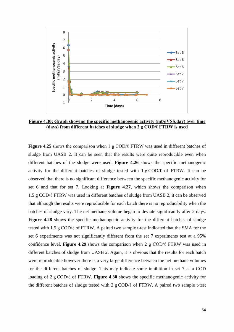
64



Figure 4.25 shows the comparison when 1 g COD/ℓ FTRW was used in different batches of

sludge from UASB 2. It can be seen that the results were quite reproducible even when

different batches of the sludge were used. Figure 4.26 shows the specific methanogenic

activity for the different batches of sludge tested with 1 g COD/ℓ of FTRW. It can be

observed that there is no significant difference between the specific methanogenic activity for

set 6 and that for set 7. Looking at Figure 4.27, which shows the comparison when

1.5 g COD/ℓ FTRW was used in different batches of sludge from UASB 2, it can be observed

that although the results were reproducible for each batch there is no reproducibility when the

batches of sludge vary. The net methane volume began to deviate significantly after 2 days.

Figure 4.28 shows the specific methanogenic activity for the different batches of sludge

tested with 1.5 g COD/ℓ of FTRW. A paired two sample t-test indicated that the SMA for the

set 6 experiments was not significantly different from the set 7 experiments test at a 95%

confidence level. Figure 4.29 shows the comparison when 2 g COD/ℓ FTRW was used in

different batches of sludge from UASB 2. Again, it is obvious that the results for each batch

were reproducible however there is a very large difference between the net methane volumes

for the different batches of sludge. This may indicate some inhibition in set 7 at a COD

loading of 2 g COD/ℓ of FTRW. Figure 4.30 shows the specific methanogenic activity for

the different batches of sludge tested with 2 g COD/ℓ of FTRW. A paired two sample t-test

-1

0

1

2

3

4

5

6

7

8

0 2 4 6 8

Spe

cifi

c m

eth

ano

gen

ic a

ctiv

ity

(mℓ

/gV

SS.d

ay)

Time (days)

Set 6

Set 6

Set 6

Set 7

Set 7

Set 7

65

indicated that the SMA for the set 7 experiments was significantly less than that for the set 6

experiments test at a 95% confidence level.

4.5. Summary

The use of additional micro-nutrients to supplement the sludge was not necessary for

experiments carried out over a short period of time since it was obvious the sludge inoculum

had sufficient micro-nutrients to last the experiment. Three methods of gas collection were

tested, the water displacement, acidified brine solution and alkaline solution methods. With

the water displacement method it was found that the gaseous carbon dioxide in the biogas

may have been dissolving in or diffusing through the displacement liquid (water) causing the

cumulative biogas volume to decrease. The acidified brine solution method lowered the

solubility of the carbon dioxide in the displacement liquid (acidified brine solution) to a

certain extent. However it was only collecting less than half of the expected biogas volume

which suggests that as the biogas volume increased, the concentration of the gaseous carbon

dioxide in the headspace increased and caused the carbon dioxide to dissolve back into the

liquid phase. Therefore the alkaline solution method was used to absorb the carbon dioxide

produced, collecting only the methane produced, which eliminated the uncertainty caused by

the carbon dioxide dynamics. The volume of methane collected using the alkaline solution

method was similar to the theoretical volume of methane expected. A concentration of

1 g COD/ℓ FTRW with UASB 2 sludge was chosen as the reference test due to its

reproducibility of the replicates within each experiment as well as its reproducibility (in

methane volume and specific methanogenic activity) across different batches of sludge.

Therefore, for the inhibition experiments, which tested the effect of SGL on the FTRW

digestion, a concentration of 1 g COD/ℓ of FTRW was used together with an additional

predetermined concentration of SGL. Additional micro-nutrients were not used to supplement

the sludge. The alkaline solution method was used to collect the methane produced.

66

CHAPTER 5

5. Effect of SGL on FTRW Digestion

In chapter 5, the effect that stripped gas liquor has on the anaerobic digestion of

Fischer-Tropsch reaction water is investigated. The aim is to test whether the stripped gas

liquor ultimately enhances or inhibits the digestion of the Fischer-Tropsch reaction water

with a sludge which is acclimated to the Fischer-Tropsch reaction water. In this chapter, it is

also determined whether there is any change in the phenol concentration during digestion. In

section 5.1, a constant concentration of 1 g COD/ℓ of Fischer-Tropsch reaction water is used,

with the stripped gas liquor contributing an additional COD loading of 0.05 and

0.15 g COD/ℓ, respectively, to the experiment. In section 5.2, the effect when a constant total

COD loading of 1 g COD/ℓ is used, with the Fischer-Tropsch reaction water contributing

85% and stripped gas liquor contributing 15% to the COD loading, is considered. Additional

micro-nutrients were not used to supplement the sludge in any of the following experiments.

The alkaline solution method was used to collect the methane produced.

Table 5-1: Table showing the concentration of the substrates and the type of gas

measurement used in the experiments to determine the effect of SGL on FTRW

digestion

Experiment Type of gas

measurement

Sodium

acetate

(g COD/ℓ)

FTRW

(g COD/ℓ)

SGL

(g COD/ℓ)

Sludge Purpose of

experiment

Set 8 Alkaline

solution

0 1 0.05, 0.15 UASB

2

Effect of SGL on

FTRW digestion

Set 9 Alkaline

solution

0 0.85 0.15 UASB

2

Effect of SGL on

FTRW digestion

67

Table 5-2: Table showing the initial characteristics of the SGL used in set 8 and 9

COD (mg/ℓ) Phenol concentration (mg/ℓ)

Set 8 2070.94 140.2

Set 9 1509.9 65.58

5.1. Set 8: Constant FTRW COD load

Set 8 tested the effect of SGL on the anaerobic digestion of FTRW. This experiment was

used to determine if there is any change in the phenol concentration in the course of the test.

The first three bottles were used as the reference units and contained 100 mℓ sludge and

1 g COD/ℓ FTRW only. The next three bottles were the test units and contained 100 mℓ

sludge, 1 g COD/ℓ FTRW and 0.05 g COD/ℓ SGL. The last three bottles were also the test

units and contained 100 mℓ sludge, 1 g COD/ℓ FTRW and 0.15 g COD/ℓ SGL. The

respective food: micro-organism ratios were 0.03, 0.034 and 0.038 g COD/g VSS. Each data

set was averaged over 3 replicates to give a mean and 95% confidence interval.

Table 5-3: Composition of test and reference units for constant FTRW load tests

Subset a and b c (5% SGL) d (15% SGL*)

Reference 1 g COD/ℓ FTRW 1 g COD/ℓ FTRW 1 g COD/ℓ FTRW

Test - (1 FTRW + 0.05 SGL) g COD/ℓ (1 FTRW + 0.15 SGL) g COD/ℓ

Duration (a) 7 d (b) 27 d 6 d 9 d

*Note: 15% SGL for set 8 is based on the COD of the reference test. When the percentage SGL was

calculated from the total COD load of the test unit it was found to be 13%. However in the discussion,

the unit test will be referred to as 15% SGL.

68


against time (days) when only 1 g COD/ℓ of FTRW is degraded and when 1 g COD/ℓ of

FTRW is co-digested with 5% SGL and 15% SGL. Reference units are labelled

according to Table 5-3

Figure 5.2: Graph showing the percentage COD recovery (%) over time (days) when

only 1 g COD/ℓ of FTRW is degraded and when 1 g COD/ℓ of FTRW is co-digested with

5% SGL and 15% SGL. Reference units are labelled according to Table 5-3

*Note: The COD recovery for the 15% SGL test [d] was much lower than the other curves due to the

fact that the VSS was lower in that experiment and therefore the rate of reaction was lower for these

test units

0

1

2

3

4

5

6

0 5 10 15 20 25 30

Cu

mu

lati

ve n

et

me

than

e p

rod

uct

ion

(m

ℓ/g

VSS

)

Time (days)

[a]

1 g COD/ℓ FTRW & 15% SGL *d+

[c]

1 g COD/ℓ FTRW & 5% SGL *c+

[d]

0

10

20

30

40

50

60

70

80

90

0 5 10 15 20 25 30

Pe

rce

nta

ge C

OD

re

cove

ry (

%)

Time (days)

1 g COD/ℓ FTRW only *b+

1 g COD/ℓ FTRW & 5% SGL *c+

1 g COD/ℓ FTRW & 15% SGL *d+* [d]*

[a]

[c]

[b]

69

Figure 5.3: Graph showing the average specific methanogenic activity (mℓ/gVSS.day)

over time (days) when only 1 g COD/ℓ of FTRW is degraded and when 1 g COD/ℓ of

FTRW is co-digested with 5% SGL and 15% SGL

Figure 5.1 shows the net cumulative methane produced over time. All test units showed

similar net methane production profiles. There is an initial exponential increase during the

first day, after which the methane production curve seems to flatten. There is then a second

increase after 5 days. Since the substrates were at room temperature before being added to the

serum bottles and placed in the water bath at 35 °C, a reasonable explanation of the initial

high, but variable calculated activity, would be thermal expansion brought about by a

decrease in the headspace temperature through addition of cooler substrates and then

reheating to the incubation temperature of 35 ºC after the units were sealed. It could also be a

period of high methanogenic activity brought about by the addition of substrate but

subsequently inhibited by pH reduction through acidogenesis.

The test units containing SGL produced similar amounts of methane to reference units. After

27 days at the sludge solids concentration used in subset d, 80% of COD had been recovered

as methane. Methane production was still continuing.

Figure 5.3 showed the specific methanogenic activity against time. The periodic increase and

decrease of the 15% test unit SMA was due to the averaging of methane volume of the

replicate bottles and the calculation of the derivative of these averages. Although the bottles

containing SGL had a higher net concentration of organics than those without SGL, this did

not translate into an increase in methanogenic activity. A paired two sample t-test was done

-1

0

1

2

3

4

5

6

0 5 10 15 20 25 30

Spe

cifi

c m

eth

ano

gen

ic a

ctiv

ity

(mℓ

/gV

SS.d

ay)

Time (days)

1 g COD/ℓ FTRW & 5% SGL


1 g COD/ℓ FTRW only

70

to compare the 5% and 15% SGL test units to the paired reference tests. This analysis was

performed only for data after the first day of the test as there may have been non-biological

effects involved in the measured gas production of the first day. The t-test indicated that the

SMA for the 5% SGL test unit was not significantly different from the SMA of the matching

1 g COD/ℓ FTRW reference test at a 95% confidence level (P = 0.103). The SMA for the

15% SGL test unit was significantly lower than for the matching 1 g COD/ℓ FTRW reference

test at a 95% confidence level (P = 9 × 10-5

) (refer to Appendix F for an example of the

calculation). This suggests that the addition of 15% SGL quantifiably reduces the SMA. It is

not possible to conclude that this is due to an inhibitory effect of SGL since the total COD

load was not the same between units with SGL and those with only FTRW. From previous

experiments it was found that there was no inhibition at higher COD loads in some batches of

sludge (Section 4.4.1. Set 6) while other batches indicated some inhibition at 2 g COD/ℓ and

above (Section 4.4.2. Set 7). However, the magnitude of the reduction in SMA suggests that

at the SGL concentrations and total COD load tested, reduction of SMA due to additional

COD load and the presence of SGL was not sufficiently great to indicate that co-digestion of

these two substrates would not be possible. This can be seen in Figure 5.1, where the net

methane production for the samples with SGL was reduced, but not dramatically so,

compared to the paired reference units.

The colorimetric analysis returns a lumped measurement of phenolic compounds. The

concentration of phenolics in the bottle with 5% SGL was measured, before the experiment

was started, as 8.53 ± 7.25 mg/ℓ and again 6 days later as 7.78 ± 6.70 mg/ℓ. The wide

confidence interval shows that the measurement is near the detection limit, and therefore the

values have limited reliability, however, the difference between these two values is not

statistically significant. The concentration of phenols in the bottle with 15% SGL was

measured, before the experiment was started, as 17.53 ± 3.07 mg/ℓ and again 7 days later as

12.1 ± 1.03 mg/ℓ. There is a significant decrease in the phenol concentration for 15% SGL.

This result suggests that conversion of phenolic compounds may be possible using a sludge

that has been acclimated to FTRW. A modification of the standards addition technique for

this analysis resulted in a smaller confidence interval in the second set of tests (Appendix E4.

Phenol measurement).

The percentage SMA reduction for the 15% SGL test unit, which had a phenol concentration

of 17.53 ± 3.07 mg/ℓ, was calculated by averaging the percentage SMA reduction at each

time (difference in the SMA as a percentage of the reference SMA) and was found to be 31%.

71

The confidence interval on the percentage reduction was difficult to calculate since there was

a high variance in the data, there was a high variance in the variance for different times and

the SMA values were derivatives of the data. However 35 observations is a significant

number of paired measurements and a confidence interval on the mean of the calculated

percentage SMA reductions at each time should give an indication of the percentage

inhibition experienced even if it may be different to the percentage inhibition in a continuous

system. The confidence interval was calculated as 20%. Therefore the percentage SMA

reduction ranged from 11 – 51%. It seems that the reduction in methanogenic activity is

significant. An alternate way to calculate the percentage SMA reduction of the 15% SGL test

unit was by comparing the average SMA difference to the average SMA of the reference and

was found to be 24% for all data after day one. This value falls in the range of 11 – 51%. The

percentage inhibition was also checked by comparing the cumulative methane produced from

day 2 to day 9 in the test unit to the cumulative methane produced in the reference unit and

was calculated to be 23% which also fall in the range of 11 – 51%. Calculations for the

percentage SMA reduction are shown in Appendix G. Therefore, despite the noisiness of the

data, several different methods of calculating the average reduction in SMA suggest that it

lay between 11 and 51% lower than the paired reference test value.

Kayembe et al. (2013) observed that 1249 ± 29.59 mg/ℓ of phenol gave a percentage

inhibition of 50% in a batch system and Fang et al. (1997) observed that the concentration of

phenol which gave a percentage inhibition of 50% ranged from 1000 to 1750 mg/ℓ in a batch

system. Assuming a linear relationship between the phenol concentration and the percentage

inhibition and using the values found in literature, the theoretical percentage inhibition for the

15% SGL test unit would range from 0.51 – 0.9%. The range of these values was much lower

than the range of the percentage SMA reductions calculated from the experiments. This

difference may be due to the different sludge types used in literature which may contain a

different mix of organisms than the sludge used in this project and thus may be able to cope

better with the sudden influx of phenol.

72

5.2. Set 9: Constant total COD load

From the previous experiments it was not possible to definitively conclude whether the

reductions in activity were due to higher COD loading or an inhibitory effect of SGL.

Therefore, in set 9, all tests had the same total COD (i.e. 1 g COD/ℓ). Tests were done in

triplicate. The blanks contained only sludge and tap water. A food: micro-organism ratio of

0.036 g COD/g VSS was used. A reference of 1 g COD/ℓ FTRW was used for comparison of

the co-digestion tests. For the co-digestion tests, the ratio of SGL to FTRW tested was 15%

SGL and 85% FTRW. The percentages were on a COD basis.

There were six extra test units set up, with the same composition as the 15% SGL test, to

sacrifice at different times during the experiment to measure phenolics, COD, VSS, pH and

for GC analysis. Since all of the additional bottles had the same initial composition as the

15% SGL test, analysis of the sacrificed bottles were assumed to be indicative of conditions

in the replicate tests.

The results from the previous experiment were used as a guide as to the approximate time

when the extra test units should be sacrificed and analysed. Looking at the results of the

previous experiments it could be seen that there were 3 critical points at which a deeper

understanding of the chemistry of the bottles would be desirable (circled in orange

on Figure 5.4 below) to understand the specific methanogenic activity curve. The additional

test units were sacrificed at each of the points indicated and analysed for COD, solids,

phenols concentration, and pH as indicated on Figure 5.4 below. The sacrificing of the

remaining 3 bottles (shown in green on Figure 5.4 below) were distributed throughout the

experiment with analysis being done more often at the beginning of the experiment and less

often as the activity slows down. Analysis for solids, pH, COD and phenolics were also done

at the beginning and end of the experiment.

73

Figure 5.4: Graph showing the proposed points and dates at which the extra bottles will

be sacrificed

For set 9, new sludge had to be grown since the sludge used in the previous experiments had

been exhausted. Sludge was originally obtained from the South African Brewery wastewater

treatment plant. This sludge was acclimated to FTRW in a UASB reactor for two months.

Since the acclimation period for the new sludge was shorter than the acclimation period for

the sludge used in set 1 – 8, the micro-organism consortium that established in the new

sludge may have been fundamentally different to the micro-organism consortium of the

previous sludge and therefore may have different biokinetic characteristics and may behave

differently with the substrates.

Accurate and frequent liquid displacement data were obtained by using webcams which

captured an image of the collection vessels every minute. All of the bottles (except those

which were sacrificed) were run to completion (i.e. until the methane production curve

flattened out and there was no further production of methane).

-1

0

1

2

3

4

5

6

0 5 10 15 20 25 30

Spe

cifi

c m

eth

ano

gen

ic a

ctiv

ity

(mℓ

/gV

SS.d

ay)

Time (days)

74


against time (days) when only 1 g COD/ℓ of FTRW is degraded and when 0.85 g COD/ℓ

of FTRW is co-digested with 0.15 g COD/ℓ of SGL

Figure 5.6: Graph showing the percentage COD recovery (%) against time (days) when

only 1 g COD/ℓ of FTRW is degraded and when 0.85 g COD/ℓ of FTRW is co-digested

with 0.15 g COD/ℓ of SGL

0

1

2

3

4

5

6

7

8

9

10

0 5 10 15 20 25 30

Cu

mu

lati

ve n

et

me

than

e p

rod

uct

ion

(m

ℓ/g

VSS

)

Time (days)

0.85 g COD/ℓ & 0.15 g COD/ℓ SGL


0

20

40

60

80

100

120

140

0 5 10 15 20 25 30

Pe

rce

nta

ge C

OD

re

cove

ry (

%)

Time (days)



75

Figure 5.7: Graph showing the specific methanogenic activity (mℓ/gVSS.day) against

time (days) when only 1 g COD/ℓ of FTRW is degraded and when 0.85 g COD/ℓ of

FTRW is co-digested with 0.15 g COD/ℓ of SGL

Figure 5.5 shows the cumulative net methane produced over time when only 1 g COD/ℓ of

FTRW was digested (reference unit) and when 0.85 g COD/ℓ of FTRW was co-digested with

0.15 g COD/ℓ of SGL (test unit). The small error bars in Figure 5.5 indicate that the three

replicates of the reference and test units showed identical behaviour. The profile of the curves

in this experiment (set 9) was much smoother than that in set 8 since the temperature of the

substrates were controlled by bringing the substrate temperature to the required temperature

of 35 °C before adding the substrates to the serum bottle. There were no step increases like

that observed in set 8 and it seemed to follow the curve of a typical Monod curve. At the

beginning of the experiment, for approximately 3 – 4 days, the methane production for both

the reference and test units were very similar. Thereafter, there was a significant difference in

the methane volumes produced, with the test unit with SGL producing more methane. There

was a decrease in the net cumulative methane curve towards the end of the reference test

which may be due to endogenous respiration as the labile substrates were exhausted and the

micro-organisms began to die. The decrease could also be due to the net methane curve in

Figure 5.5 being calculated from a difference between the methane production of the test unit

and the methane production of the blank. The percentage COD recovery was determined by

converting the volume of gas collected (assumed to be methane only) to g COD and

comparing it to the initial quantity of food added to the bottle. The percentage COD recovery

-2

-1

0

1

2

3

4

5

6

7

8

0 5 10 15 20 25 30

Spe

cifi

c m

eth

ano

gen

ic a

ctiv

ity

(mℓ

/gV

SS.d

ay)

Time (days)



76

for both the reference and test units were above 100% as shown in Figure 5.6. This may be

due to sludge stimulation which caused an enhanced degradation of slowly degradable

material that may have been present in the sludge from the previous use of the sludge or the

degradation of products resulting from biomass death. The specific methanogenic activity is

shown in Figure 5.7 and it could be observed that the specific methanogenic activity of the

reference unit was significantly lower than that of the test unit. A paired two sample t-test

confirmed this difference with P = 3.8 × 10-5

. The analysis was performed with data from

day 0 to day 24. Therefore there was no evidence of SMA reduction by the addition of SGL.

There may even have been some stimulation of the anaerobic activity as a result of the

presence of different labile substrate constituents in the sludge. The reduction in the specific

methanogenic activity of the test unit in the previous experiment (set 8) may have been due to

the higher COD loading rather than an inhibitory effect of SGL. However previous

experiments found that there was no inhibition at higher COD loads in some batches of

sludge (Section 4.4.1. Set 6) while other batches indicated some inhibition at 2 g COD/ℓ and

above (Section 4.4.2. Set 7). Therefore the suggestion that the apparent reduction in the

activity in set 8 may be due to the increased COD load instead of the inhibitory effect of SGL

is not strongly supported. The SGL used in set 8 and set 9 were from different batches and

had different COD and phenol concentrations. The SGL used in set 8 had a higher COD and

phenol concentration than that used in set 9 as shown in Table 5-2. The phenol concentration

of the SGL used in set 9 was 65.58 mg/ℓ while the phenol concentration of the SGL used in

set 8 was 140.2 mg/ℓ, which was more than twice the concentration of the set 9 SGL.

Therefore it was concluded the addition of SGL potentially reduced the SMA and that this

could be an inhibitory effect, but that any inhibition would be a function of the concentration

of potentially inhibitory substances in SGL and that these concentrations vary from batch to

batch. However, even if the SGL is inhibitory at the 15% SGL level with a total COD load of

1.15 g COD/ℓ, the degree of inhibition is fairly low and would not prevent co-digestion of the

two streams at the concentrations tested. The mechanism of inhibition is unknown at this

stage and determining the mechanism of inhibition would require much more complex,

expensive and time-consuming experiments that were outside the scope of the project.

The pH, VSS, COD and phenol concentration of the test units (0.85 g COD/ℓ FTRW and

0.15 g COD/ℓ SGL) were measured during the experiment.

77

Figure 5.8: Graph showing the pH value against time (days) for the test unit with

0.85 g COD/ℓ of FTRW co-digested with 0.15 g COD/ℓ of SGL

Figure 5.8 showed the pH of the test unit at intervals during the experiment. All

measurements were made from different but identically constituted bottles. The pH remained

between 6.5 and 7.5 which is the optimum pH range for anaerobic digestion (Liu et al.,

2007).

Figure 5.9: Graph showing the volatile suspended solids (mg/ℓ) against time (days) for

the test unit with 0.85 g COD/ℓ of FTRW co-digested with 0.15 g COD/ℓ of SGL

6

6.2

6.4

6.6

6.8

7

7.2

7.4

0 5 10 15 20 25 30

pH

Time (days)

0

5000

10000

15000

20000

25000

0 5 10 15 20 25 30

VSS

(m

g/ℓ

)

Time (days)

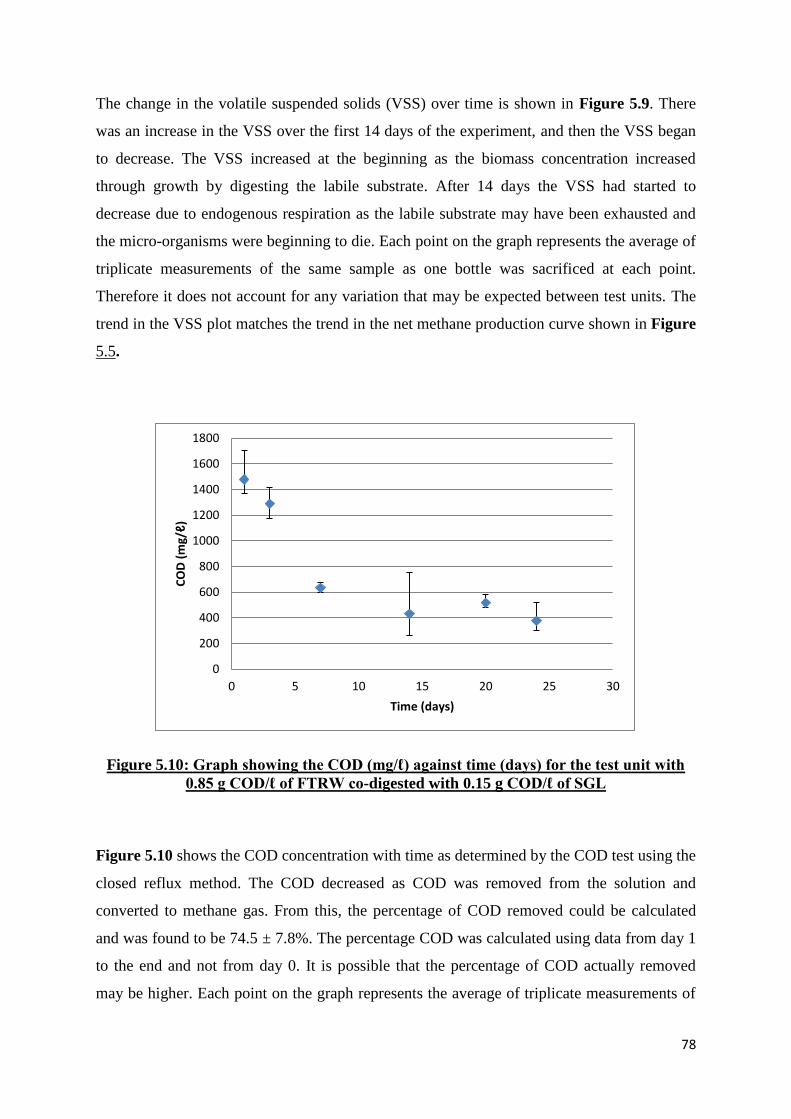
78

The change in the volatile suspended solids (VSS) over time is shown in Figure 5.9. There

was an increase in the VSS over the first 14 days of the experiment, and then the VSS began

to decrease. The VSS increased at the beginning as the biomass concentration increased

through growth by digesting the labile substrate. After 14 days the VSS had started to

decrease due to endogenous respiration as the labile substrate may have been exhausted and

the micro-organisms were beginning to die. Each point on the graph represents the average of

triplicate measurements of the same sample as one bottle was sacrificed at each point.

Therefore it does not account for any variation that may be expected between test units. The

trend in the VSS plot matches the trend in the net methane production curve shown in Figure

5.5.

Figure 5.10: Graph showing the COD (mg/ℓ) against time (days) for the test unit with

0.85 g COD/ℓ of FTRW co-digested with 0.15 g COD/ℓ of SGL

Figure 5.10 shows the COD concentration with time as determined by the COD test using the

closed reflux method. The COD decreased as COD was removed from the solution and

converted to methane gas. From this, the percentage of COD removed could be calculated

and was found to be 74.5 ± 7.8%. The percentage COD was calculated using data from day 1

to the end and not from day 0. It is possible that the percentage of COD actually removed

may be higher. Each point on the graph represents the average of triplicate measurements of

0

200

400

600

800

1000

1200

1400

1600

1800

0 5 10 15 20 25 30

CO

D (

mg/

ℓ)

Time (days)

79

the same sample as one bottle was sacrificed at each point. Therefore it does not account for

any variation that may be expected between test units.

The phenols were analysed by the colorimetric method and the gas chromatograph.

Figure 5.11: Graph showing the phenol concentration (mg/ℓ) against time (days) for the

test unit with 0.85 g COD/ℓ of FTRW co-digested with 0.15 g COD/ℓ of SGL

Figure 5.11 shows the phenol concentration results from the colorimetric method. At the

beginning of the experiment the phenol concentration was 8.21 ± 0.91 mg/ℓ and at the end of

the experiment it was 6.49 ± 0.67 mg/ℓ. There was a decrease in the concentration of the

phenols in the test unit from the beginning of the experiment to the end and the two values

were significantly different, but only by a very small amount. While some removal may

occur, the percentage phenol removal appears to be a lot lower than the percentage COD

removal, suggesting that even if phenols are degraded, the sludge is not effective for phenol

removal.

0

2

4

6

8

10

12

14

16

18

0 5 10 15 20 25 30

Ph

en

ol c

on

cen

trat

ion

(m

g/ℓ

)

Time (days)

80


beginning of the experiment (day 1)


end of the experiment (day 23)

0.25 0.50 0.75 1.00 1.25 1.50 1.75 2.00 2.25 2.50 2.75 3.00 3.25 3.50 3.75 4.00 4.25 4.50 4.75 min

0.00

0.25

0.50

0.75

1.00

1.25

1.50

1.75

2.00

2.25

uV(x10,000,000)

0

50

100

150

200

250

300

350

400

C

Column Temp.(Setting)Chromatogram

0.25 0.50 0.75 1.00 1.25 1.50 1.75 2.00 2.25 2.50 2.75 3.00 3.25 3.50 3.75 4.00 4.25 4.50 4.75 min

0.00

0.25

0.50

0.75

1.00

1.25

1.50

1.75

2.00

2.25

uV(x10,000,000)

0

50

100

150

200

250

300

350

400

C

Column Temp.(Setting)Chromatogram

81

Figure 5.14: Overlap of the gas chromatograph profiles of the test unit at the beginning

(orange) and end of the experiment (black)

The concentration of the phenol in the test unit test was also analysed using a gas

chromatograph. A solid phase extraction was performed before GC analysis. During the solid

phase extraction there were a number of steps where uncertainty may have been introduced

and with the heterogeneous nature of the samples it was not possible to obtain a high enough

precision on the standard samples to be confident in the calibration curve. Therefore the

chromatograph profiles have been used for a qualitative validation of the results obtained

from the colorimetric method. An analysis of a pure phenol solution showed that the retention

time for the phenol peak was around 2.4 minutes. Figure 5.12 and Figure 5.13 show the gas

chromatograph profiles of the test unit at the beginning and end of the experiment,

respectively. An overlay of the gas chromatograph profiles (Figure 5.14) showed that there

was no significant difference in the phenol peaks and therefore little change in the phenol

concentration during the experiment.

82

CHAPTER 6

6. Discussion

The purpose of this study was to determine the influence of stripped gas liquor on the specific

methanogenic activity of Fischer-Tropsch reaction water acclimated sludge and to investigate

the fate of indicator compounds for potentially toxic higher molecular weight organics in

stripped gas liquor, such as phenols, in batch anaerobic co-digestion experiments. In order to

determine this, serum bottle tests were performed under mesophilic conditions to measure the

methanogenic activity when Fischer-Tropsch reaction water and stripped gas liquor are

anaerobically co-digested. The biogas produced was collected and monitored during the

experiments. This chapter discusses the experimental results obtained with regards to the

research outcomes.

6.1. Method development

The method development chapter investigated whether the use of additional nutrients was

necessary and evaluated techniques to collect and measure the biogas produced. Different

COD loads of the FTRW were tested to determine what the base experiment should look like

and a reference test was chosen.

6.1.1. The necessity of additional nutrients

It was found early in the method development that the use of additional micro-nutrients to

supplement the sludge was not necessary for experiments carried out over a short period of

time since the biogas produced was similar in the test units with and without additional

nutrients. It was obvious the sludge inoculum had sufficient micro-nutrients to last the

experiment. Therefore nutrients were not added to subsequent serum bottle tests.

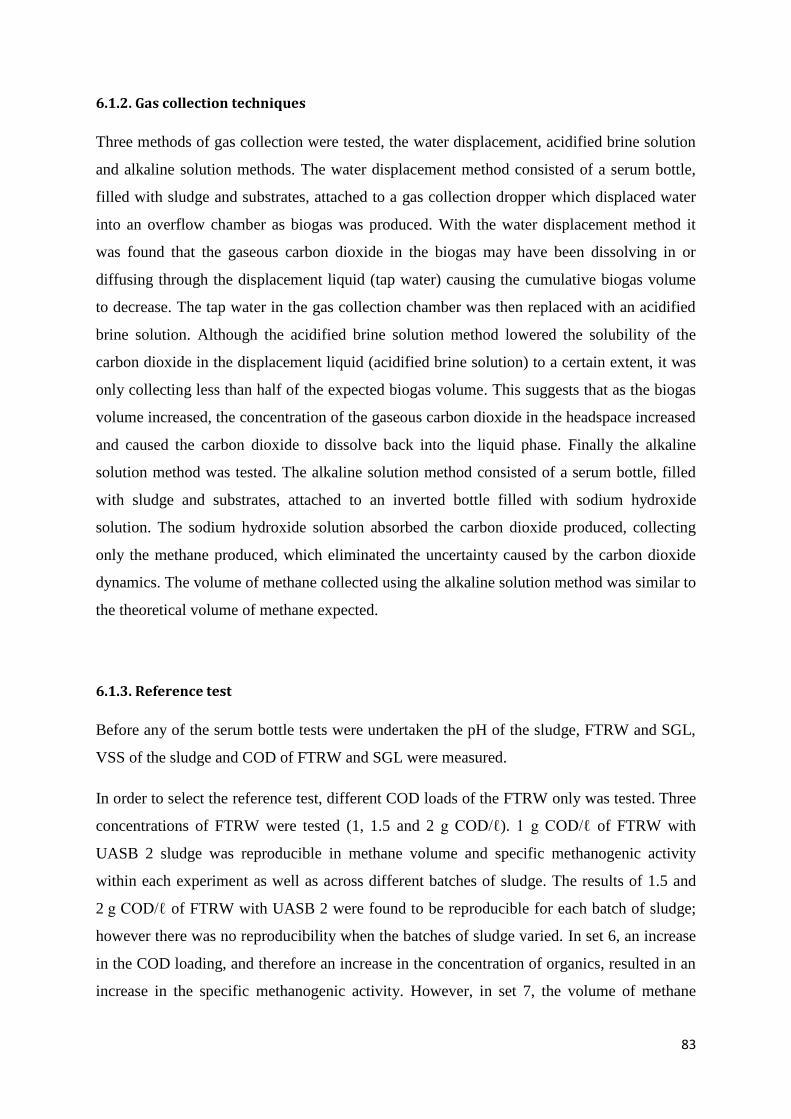
83

6.1.2. Gas collection techniques

Three methods of gas collection were tested, the water displacement, acidified brine solution

and alkaline solution methods. The water displacement method consisted of a serum bottle,

filled with sludge and substrates, attached to a gas collection dropper which displaced water

into an overflow chamber as biogas was produced. With the water displacement method it

was found that the gaseous carbon dioxide in the biogas may have been dissolving in or

diffusing through the displacement liquid (tap water) causing the cumulative biogas volume

to decrease. The tap water in the gas collection chamber was then replaced with an acidified

brine solution. Although the acidified brine solution method lowered the solubility of the

carbon dioxide in the displacement liquid (acidified brine solution) to a certain extent, it was

only collecting less than half of the expected biogas volume. This suggests that as the biogas

volume increased, the concentration of the gaseous carbon dioxide in the headspace increased

and caused the carbon dioxide to dissolve back into the liquid phase. Finally the alkaline

solution method was tested. The alkaline solution method consisted of a serum bottle, filled

with sludge and substrates, attached to an inverted bottle filled with sodium hydroxide

solution. The sodium hydroxide solution absorbed the carbon dioxide produced, collecting

only the methane produced, which eliminated the uncertainty caused by the carbon dioxide

dynamics. The volume of methane collected using the alkaline solution method was similar to

the theoretical volume of methane expected.

6.1.3. Reference test

Before any of the serum bottle tests were undertaken the pH of the sludge, FTRW and SGL,

VSS of the sludge and COD of FTRW and SGL were measured.

In order to select the reference test, different COD loads of the FTRW only was tested. Three

concentrations of FTRW were tested (1, 1.5 and 2 g COD/ℓ). 1 g COD/ℓ of FTRW with

UASB 2 sludge was reproducible in methane volume and specific methanogenic activity

within each experiment as well as across different batches of sludge. The results of 1.5 and

2 g COD/ℓ of FTRW with UASB 2 were found to be reproducible for each batch of sludge;

however there was no reproducibility when the batches of sludge varied. In set 6, an increase

in the COD loading, and therefore an increase in the concentration of organics, resulted in an

increase in the specific methanogenic activity. However, in set 7, the volume of methane

84

produced in the bottles testing 2 g COD/ℓ of FTRW was much lower than that produced in

the bottles with 1 and 1.5 g COD/ℓ of FTRW. This may indicate some inhibition in this batch

of sludge with a COD loading of 2 g COD/ℓ of FTRW.

Therefore, for the inhibition experiments, which tested the effect of SGL on the FTRW

digestion, a concentration of 1 g COD/ℓ of FTRW was used together with an additional

predetermined concentration of SGL. Additional micro-nutrients were not used to supplement

the sludge. The alkaline solution method was used to collect the methane produced.

6.2. Effect of SGL on FTRW digestion

Chapter 5 investigated whether the stripped gas liquor would enhance or inhibit the digestion

of the Fischer-Tropsch reaction water with a sludge which was acclimated to the

Fischer-Tropsch reaction water and whether there would be any change in the phenol

concentration during digestion.

6.2.1. Constant FTRW COD load (Set 8)

A concentration of 1 g COD/ℓ of FTRW only was used as the reference unit. For the test

units, a constant concentration of 1 g COD/ℓ of FTRW was used, with the SGL contributing

an additional COD loading of 0.05 g COD/ℓ (5% SGL) and 0.15 g COD/ℓ (15% SGL),

respectively, to the experiment. This gave the test units total COD loadings of 1.05 g COD/ℓ

and 1.15 g COD/ℓ, respectively. The SMA for the 5% SGL test unit was not significantly

different from the SMA of the matching 1 g COD/ℓ FTRW reference test. The SMA for the

15% SGL test unit was significantly lower than for the matching 1 g COD/ℓ FTRW reference

test. This suggested that the addition of 15% SGL quantifiably reduced the SMA. However it

was not possible to conclude whether this was due to an inhibitory effect of SGL or a higher

COD loading since the total COD load was not the same between the test units with SGL and

the reference unit with only FTRW. Previous experiments showed that there was no

inhibition at higher COD loads in some batches of sludge (Section 4.4.1. Set 6) while other

batches indicated some inhibition at 2 g COD/ℓ and above (Section 4.4.2. Set 7).

The colorimetric analysis was performed at the beginning and end of the experiment to

determine whether the phenol concentration had decreased during the anaerobic digestion of

85

FTRW and SGL. For the 5% SGL test unit, the difference between the two values was not

statistically significant. There was a significant but small decrease in the phenol

concentration for the 15% SGL test unit. This result suggested that conversion of phenolic

compounds may be possible using a sludge that has been acclimated to FTRW. However the

reduction of phenol was lower than the reduction of COD.

6.2.2. Constant total COD load (Set 9)

In this experiment the total COD load was kept constant at 1 g COD/ℓ. The reference test was

1 g COD/ℓ FTRW only. The test unit consisted of 85% FTRW (0.85 g COD/ℓ) and 15% SGL

(0.15 g COD/ℓ). This was to determine whether the reduction in the SMA in the previous

experiment was due to an inhibitory effect of SGL or an increase in the COD load. Although

in set 9 the total COD load was kept constant in order to make comparison of results simpler,

it is not the only option. The acetate concentration could be kept constant by calculating the

acetate contribution from SGL and FTRW and ensuring that each of the replicates added up

to a constant value. A constant low molecular weight organics concentration can be

calculated in a similar manner.

It was found that the SMA of the test unit was higher than that of the reference unit.

Therefore there seemed to be no inhibition by SGL when the COD load was kept constant.

This suggested that the reduction in SMA in the test unit in the previous experiment may

have been due to an increase in the COD load when SGL was added over and above the

1 g COD/ℓ of FTRW. However, it could also have been due to a fundamental difference

between the two batches of SGL since they had different COD and phenol concentrations.

The SGL used in set 8 had a higher COD and phenol concentration than that used in set 9.

The phenol concentration of the SGL used in set 8 was more than twice the phenol

concentration of the set 9 SGL.

The pH, VSS, COD and phenol concentration of the test units were measured regularly

during the experiment. The pH remained within the optimum pH range of 6.5 and 7.5. The

VSS increased as more biomass was produced. Then after 14 days the VSS began to decrease

due to endogenous respiration as the labile substrate was exhausted and the micro-organisms

began to die. The COD decreased as it was removed from solution and converted to methane

gas. 74.5 ± 7.8% of COD was removed between day 1 and the end of the test. The overall

86

percentage COD removed between day 0 and the end of the test would be higher. The

colorimetric method and the gas chromatograph profiles showed that there was little decrease

in the phenol concentration during the test.

6.3. Hypotheses

The first hypothesis was that the anaerobic sludge, which was acclimated to Fischer-Tropsch

reaction water only, would be inhibited by the higher molecular weight organics such as

phenols in stripped gas liquor. The results from Chapter 5 (Effect of SGL on FTRW

Digestion) were ambiguous in terms of the first hypothesis. This may be due to the

differences in the SGL batches between the two sets of experiments (set 8 and 9). Set 8

supports the first hypothesis, but not conclusively since the COD load was varying between

the reference and test units. Set 9 does not support the first hypothesis since there was no

evidence of inhibition by the SGL. Therefore it has not been proven that SGL will not be

inhibitory, but it has been shown that FTRW digestion can occur in the presence of SGL and

that certain components of the SGL can be degraded (as shown by the higher methanogenic

activity in the test units in set 9). The percentage reduction in methanogenic activity of the

15% SGL test units ranged from 11% to 51% for set 8 and there was no inhibition in set 9.

This suggests that any reduction in SMA due to additional SGL at concentrations and

SGL:FTRW ratios tested was between 0 and 51%. However, the phenolic compounds in the

SGL used in this project had a larger range of SMA reduction percentages than that found in

literature. This difference may be due to the different sludge types used in literature which

may contain a different mix of organisms than the sludge used in this project and thus may be

able to cope better with a sudden influx of phenol.

The second hypothesis was that the Fischer-Tropsch reaction water acclimated sludge would

not be able to degrade the phenolics in stripped gas liquor. Set 8 does not seem to support the

second hypothesis since a significant decrease in the phenol concentration was observed after

7 days of incubation with the FTRW-acclimated sludge. However, percentage wise, the

phenol reduction was lower than the COD removal. In set 9, the second hypothesis seems to

be supported in that there was very little change in the measured phenol concentration after

24 days of incubation with the FTRW-acclimated sludge. However, the results are again not

conclusive because of the high variance between values. However again, the percentage

decrease in the phenol concentration is small compared to the percentage decrease in COD.

87

By looking at the variance between the samples in set 9, it could be seen that there can be

quite a large difference between samples, but no evidence overall that the phenol

concentration was decreasing.

At the COD blend ratios tested during this project, anaerobic digestion proceeds adequately.

However, there is evidence that certain components present in SGL cannot be degraded or are

degraded slowly. The sludge will have to be acclimated to SGL if these constituents are to be

degraded in the co-digester. In a continuous digester which is appropriately seeded and

acclimated to SGL, much higher rates of phenol removal might be observed.

The experimental method used in this project has certain limitations. The serum bottle

technique used was only a batch process and could not accurately represent the behaviour of

the micro-organisms in a continuous process. The serum bottles were small and could only

accommodate a limited volume of biomass and substrates. The NaOH collection system also

had limitations as it had to be emptied while the reaction was still continuing whenever it

filled up too much. However, the experimental method was sufficient for the requirements of

this project as it is just the first step in the broader project of FTRW and SGL co-digestion.

The experiments in this project gave an indication of the inhibition of the FTRW digestion by

SGL. The results from this project can be used to design, model and select possible

continuous experiments at 15% SGL and higher since it is impossible to physically try every

option. The inhibition for the continuous experiments can then be measured. The “worst case

scenario” of percentage SMA reduction values can be used in a model for a conservative

experiment design. It is recommended that a sensitivity analysis be performed using a range

of SMA reduction values to observe how differences in this value influence the possible

range of operating conditions of a continuous co-digester.

88

CHAPTER 7

7. Conclusions and Recommendations

This project was set out to investigate the effect that stripped gas liquor had on the

Fischer-Tropsch reaction water anaerobic digestion by determining the influence of stripped

gas liquor on the specific methanogenic activity of Fischer-Tropsch reaction water acclimated

sludge and by evaluating the fate of indicator compounds for potentially toxic higher

molecular weight organics in stripped gas liquor, such as phenols, in batch anaerobic

co-digestion experiments. The serum bottle was used as a batch reactor and the biogas

production was monitored to measure the extent of the degradation.

It was hypothesised that (i) the anaerobic sludge, which was acclimated to Fischer-Tropsch

reaction water only, would be inhibited by the higher molecular weight organics such as

phenols in stripped gas liquor; and (ii) the Fischer-Tropsch reaction water acclimated sludge

would not be able to degrade the phenolics in stripped gas liquor.

This chapter presents the conclusions relating to the experiment design and the hypotheses. It

also gives recommendations that may be useful in future research.

7.1. Conclusions

The use of additional nutrients to supplement the sludge was not necessary for

experiments carried out over a short time period.

A method was investigated to successfully collect the biogas produced. The alkaline

solution displacement method, which absorbed the carbon dioxide produced and

collected only the methane, was selected to collect and measure the biogas produced

since it eliminated the uncertainties arising from the carbon dioxide dynamics.

A concentration of 1 g COD/ℓ FTRW was chosen as the reference test due to its

reproducibility of the replicates within each experiment as well as its reproducibility

89

(in methane volume and specific methanogenic activity) across different batches of

sludge.

From the results of the co-digestion it was concluded that the addition of SGL

potentially reduced the SMA and that this could be an inhibitory effect, but that any

inhibition would be a function of the concentration of potentially inhibitory

substances in SGL and that these concentrations vary from batch to batch. However,

even if the SGL is inhibitory at the 15% SGL level with a total COD load of

1.15 g COD/ℓ, the degree of inhibition is fairly low and would not prevent

co-digestion of the two streams at the concentrations tested.

There was a significant but small decrease in the phenol concentration. Therefore it

was concluded that the Fischer-Tropsch reaction water acclimated sludge may be able

to degrade some of the phenolics in stripped gas liquor but the measured percentage

removal of phenol was lower than the measure percentage COD removal.

In terms of the first hypothesis (the anaerobic sludge, which is acclimated to

Fischer-Tropsch reaction water only, will be inhibited by the higher molecular weight

organics such as phenols in stripped gas liquor) it has not been proven that SGL will

not be inhibitory, but it has been shown that FTRW anaerobic digestion can proceed

adequately in the presence of SGL. The percentage SMA reduction observed ranged

from 0 – 51% for the 15% SGL test units, however it is anticipated that much lower

ranges would be observed in a continuous system. Literature and set 9 suggest that the

actual SMA reduction due to potentially inhibitory organic compounds in the SGL

may be negligible.

In terms of the second hypothesis (the Fischer-Tropsch reaction water acclimated

sludge will not be able to degrade the phenolics in stripped gas liquor) there was some

evidence that phenolics were degraded but at a much slower rate than COD.

90

7.2. Recommendations

In future research it is recommended that some way be developed to take samples of the gas

collected above the alkaline solution method in the inverted bottle during the experiment. The

samples can then be analysed in a gas chromatograph to ensure that only methane is present

to eliminate the possibility that air may diffuse into the inverted bottle and cause incorrect gas

measurements.

The results from this project can be incorporated into a simple co-digestion model which

could later be used to design continuous experiments at a range of FTRW:SGL ratios. The

inhibition can then be measured for the continuous experiments. It is recommended that a

sensitivity analysis be performed using a range of SMA reduction values to observe how

differences in this value influence the possible range of operating conditions of a continuous

co-digester.

Experiments can be conducted to determine the mechanism of inhibition.

The experiments in this project found that there was a very small decrease in the phenol

concentration when stripped gas liquor was anaerobically digested by Fischer-Tropsch

reaction water acclimated sludge. Therefore it may be useful to acclimatise the sludge to

stripped gas liquor instead (Chen et al., 2007), by using a gradual start-up and slowly

introducing the higher molecular weight organics so that the micro-organisms that are

capable of metabolising these organics can become well-established.

This project is only the first step of the development of a co-digestion model relating organic

loading rate, SGL: FTRW feed ratio to methane recovery and extent of biodegradation of

phenol for use in the design and optimization of a co-digestion system. There is some

indication of how SGL and the higher molecular weight organics, such as phenols, in SGL

may affect FTRW digestion and an indication of percentage SMA reduction that may be

experienced. The results from this project can be incorporated into a simple co-digestion

model, together with results from future projects investigating the digestion of SGL, to design

and model continuous experiments from which the inhibition can be measured. This will

contribute to the investigation of the co-digestion of stripped gas liquor and Fischer-Tropsch

reaction water.

91

References

1. Aldin S. (2010), The Effect of Particle Size on Hydrolysis and Modelling of Anaerobic

Digestion, Department of Chemical and Biochemical Engineering, University of

Western Ontario, Ontario, pages 15 - 16

2. Bagudo B.U., Garba B., Dangoggo S.M. and Hassan L.G. (2011), The Qualitative

Evaluation of Biogas Samples Generated from Selected Organic Wastes, Archives of

Applied Science Research, Volume 3, No. 5, pages 549 – 555

3. Batstone D. J., Keller J., Angelidaki R. I., Kalyuzhnyi S. V., Pavlostathis S. G., Rozzi

A., Sanders W. T. M., Siegrist H. and Vavilin V. A. (2002), Anaerobic Digestion

Model No. 1 (ADM1) Scientific and Technical Report No.13 IWA Task Group for

Mathematical Modelling of Anaerobic Wastewater, IWA publishing, London, pages

13 - 25

4. Beccari M., Majone M., Dionisi D., Dionisi A., Addario E.N.D. and Sbardellati R.

(2006), High-rate Anaerobic-aerobic Biological Treatment of a Wastewater from a

Fischer-Tropsch Process, Sapienza University of Rome, Dept of Chemistry and Eni

S.p.A, Refining and Marketing Division, Italy

5. Beychok M.R. (1975), Coal Gasification and the Phenosolvan Process, Irvine,

California, pages 86 – 87

6. Brady III R.C. and Pettit R. (1981), Mechanism of the Fischer-Tropsch reaction. The

chain propagation step, American Chemical Society, Volume 5, No. 103,

pages 1287 - 1289

7. Chen Y., Cheng J.J. and Creamer K.S. (2007), Inhibition of Anaerobic Digestion

Process: A Review, Bioresource Technology, Volume 99, pages 4044 – 4064

8. Conklin A.S., Chapman T., Zahller J.D., Stensel H.D. and Ferguson J.F. (2008),

Monitoring the Role of Aceticlasts in Anaerobic Digestion: Activity and Capacity,

Water Research, Volume 42, pages 4895 - 4904

92

9. Crueger W. and Crueger A. (1990), Biotechnology: A Textbook of Industrial

Microbiology, second edition, Science Tech Publishers, United States of America,

pages 317 - 324

10. Dannis M. (1951), Determination of Phenols by the Amino-Antipyrine Method,

Sewage and Industrial Wastes, Water Environment Federation, Volume 23, No. 12,

pages 1516 - 1522

11. Davies O.L. and Goldsmith P.L. (1977), Statistical methods in research and

production, 4th edition, Longman Group Limited, London

12. Dhadse S., Kankal N.C. and Kumari B. (2012), Study of Diverse Methanogenic and

Non-methanogenic Bacteria Used for the Enhancement of Biogas Production,

International Journal of Life Sciences Biotechnology and Pharma Research,

Volume 1, No. 2

13. Dochain D. and Vanrolleghem P.A. (2001), Dynamical Modelling and Estimation in

Wastewater Treatment Processes, IWA Publishing, London, UK, pages 197 - 201

14. Donaldson T.L., Lee D.D. and Singh S.P.N. (1987), Treatment of Coal Gasification

Wastewaters, Oak Ridge National Laboratory, Martin Marietta Energy Systems Inc.,

United States of America

15. Donoso-Bravo A., Pérez-Elvira S., Aymerich E. and Fdz-Polanco F. (2011),

Assessment of the Influence of Thermal Pre-Treatment Time on the Macromolecular

Composition and Anaerobic Biodegradability of Sewage Sludge, Bioresource

Technology, Volume 102, pages 660–666

16. Emerson E. (1943), The Condensation of Aminoantipyrine: II. A New Colour Test for

Phenolic Compounds, Chemical Laboratory, Trinity College

17. Ettinger M.B., Ruchhoft C.C. and Lishka R.J. (1951), Sensitive 4-Aminoantipyrine

Method for Phenolic Compounds, Analytical Chemistry, Volume 23, No. 12,

pages 1783 – 1788

93

18. Esposito G., Frunzo L., Liotta F., Panico A. and Pirozzi F. (2012), Biomethane

potential tests to measure the biogas production from the digestion and co-digestion

of complex organic substrates, The Open Environmental Engineering Journal,

Volume 5, pages 1 – 8

19. Fang H.H.P. and Chan O. (1997), Toxicity of Phenol Towards Anaerobic Biogranules,

Water Research, Volume 31, No. 9, pages 2229 – 2242

20. Farbiszewska T., Farbiszewska-Kiczma J., Jazdzyk E., Sadowski Z. and Szubert A.

(2006), Kinetic Study of Biodegradation of Organic Matter Extracted from Black

Shale Ore, Physicochemical Problems of Mineral Processing, Volume 40,

pages 317 – 325

21. Foxon K.M. (2009), Analysis of a Pilot-Scale Anaerobic Baffled Reactor Treating

Domestic Wastewater, School of Chemical Engineering, University of KwaZulu

Natal, South Africa

22. Gerber M. and Span R. (2008), An Analysis of Available Mathematical Models for

Anaerobic Digestion of Organic Substances for Production of Biogas, International

Gas Union Research Conference, Paris, pages 10 – 11

23. Girish C.R. and Murty V.R. (2012), Adsorption of Phenol from Wastewater using

Locally Available Adsorbents, Journal of Environmental Research and Development,

Volume 6, No. 3A, 763 – 772

24. Goldman A.D., Leigh J.A. and Samudrala R. (2009), Comprehensive Computational

Analysis of Hmd Enzymes and Paralogs in Methanogenic Archea, BMC Evolutionary

Biology, Volume 9, Issue 199

25. Gottlieb S. and Marsh P.B. (1946), Quantitative Determination of Phenolic

Fungicides, Industrial and Engineering Chemistry, Volume 18, No. 1, pages 16 – 19

26. Hippeli E.M. (1955), Exogenous and Endogenous Respiration in Microorganisms,

United States Naval Postgraduate School, Monterey, California

27. Iyagba E.T., Mangibo I.A. and Mohammad Y.S. (2009), The Study of Cow Dung as

Co-substrate with Rice Husk in Biogas Production, Scientific Research and Essay,

Volume 4, No. 9, pages 861 – 866

94

28. Kayembe K., Basosila L., Mpiana P.T., Sikulisimwa P.C. and Mbuya K. (2013),

Inhibitory Effects of Phenolic Monomers on Methanogenesis in Anaerobic Digestion,

British Microbiology Research Journal, No. 3, pages 34 – 41

29. Kupiec T. (2004), Quality-Control Analytical Methods: Gas Chromatography,

International Journal of Pharmaceutical Compounding, Volume 8, No. 4,

pages 305 – 309

30. Lettinga G. (1995), Anaerobic Digestion and Wastewater Treatment Systems, Antonie

van Leeuwenhoek, Volume 67, pages 3 – 28

31. Liu C., Yaun X., Zeng G., Li W. and Li J. (2008), Prediction of Methane Yield at

Optimum pH for Anaerobic Digestion of Organic Fraction of Municipal Solid Waste,

Bioresource Technology, Volume 99, pages 882 – 888

32. Lokshina L., Vavilin V.A., Kettunen R.H., Rintala J.A., Holliger C. and

Nozhevnikova A.N. (2001), Evaluation of Kinetic Coefficients Using Integrated

Monod and Haldane Models for Low-Temperature Acetoclastic Methanogenesis,

Water Research, Volume 35, No. 12, pages 2913 – 2922

33. Martin R.W. (1949), Rapid Colorimetric Estimation of Phenol, Analytical Chemistry,

Volume 21, No. 11, pages 1419 – 1420

34. Moody L., Burns R., Wu-Haan W and Spajić R. (2008), Use of Biochemical Methane

Potential (BMP) Assays for Predicting and Enhancing Anaerobic Digester

Performance, 44th

Croatian and 4th

International Symposium on Agriculture, Croatia,

pages 930 - 934

35. Nwaneri C.F. (2009), Physico-Chemical Characteristics and Biodegradability of

Contents of Ventilated Improved Pit Latrines (VIPS) in Ethekwini Municipality,

School of Biological and Conservation sciences, University of KwaZulu Natal,

pages 43 – 50

36. Ochynski F.W. (1960), The Absorptiometric Determination of Phenol, Department of

Scientific and Industrial Research, National Chemical Laboratory, Teddington,

Middlesex

95

37. Owen W.F., Stuckey D.C., Healy J.B, Young L.Y. and McCarty P.L. (1979),

Bioassay for Monitoring Biochemical Methane Potential and Anaerobic Toxicity,

Water Research, Volume 13, Pergamon Press, New York, pages 485 – 492

38. Parajuli P. (2011), Biogas Measurement Techniques and the Associated Errors,

Department of Biological and Environmental Science, University of Jyvӓskylӓ,

Finland

39. Park H.M. (2009), Comparing Group Means: T-tests and One-way ANOVA Using

Stata, SAS, R and SPSS*, University Information Technology Services Center for

Statistical and Mathematical Computing, Indiana University

40. Reddy P. (2008), Environmental Impact Report for the Water Recovery Growth

Project, Sasol Synfuels, Mpumalanga Province, Bohlweki-SSI Environmental

41. Remigi E. and Buckley C.A. (2006), Co-Digestion of High Strength/ Toxic Organic

Effluents in Anaerobic Digesters at Wastewater Treatment Works. Water Research

Commission Report in Preparation, South Africa

42. Remigi E. and Buckley C.A. (2006), Anaerobic Digestion for the Treatment of Toxic

and High Strength Organic Wastes : A Case Study in eThekwini Municipality,

Research report K5/1538, Water Research Commission, Pretoria, South Africa

43. Remigi E., Dlamini S. and Buckley C. (2006), Verification of a Protocol for the

Assessment of the Disposal of Industrial Organic Waste by Co-Digestion, Pollution

Research Group, University of KwaZulu Natal

44. School of Chemical Engineering (2007), A Guide to Serum Bottle Tests, Howard

College Campus, University of KwaZulu Natal

45. Shelton D.R. and Tiedjie J.M. (1984), General Method for Determining Anaerobic

Biodegradation Potential, Michigan Agricultural Experiment Station, Journal Article

No. 11032, pages 850 – 857

46. Snoeyink V.L. and Jenkins D. (1980), Water Chemistry, John Wiley & Sons, New

York

96

47. Stieb M. and Schink B. (1985), Anaerobic Oxidation of Fatty Acids by Clostridium

Bryantii sp. nov., a Sporeforming, Obligately Syntrophic Bacterium, Archives of

Microbiology, No. 140, pages 387 – 390

48. Walker M., Zhang Y., Heaven S. and Banks C. (2009), Potential Errors in the

Quantitative Evaluation of Biogas Production in Anaerobic Digestion Processes,

Bioresource Technology, Volume 100, No. 24, pages 6339 – 6346

49. Wiseman A. (1978), Topics in Enzyme and Fermentation Biotechnology 2, Ellis

Horwood Limited, England, pages 202 - 271

50. Wu W. (2007), Anaerobic Co-Digestion of Biomass for Methane Production: Recent

Research Achievements, Iowa State University, United States of America, pages 1 – 2

51. Van Zyl P.J. (2008), Anaerobic Digestion of Fischer-Tropsch Reaction Water:

Submerged Membrane Anaerobic Reactor Design, Performance Evaluation &

Modelling, Water Research Group, Department of Civil Engineering, University of

Cape Town, pages 86 - 88 and 230

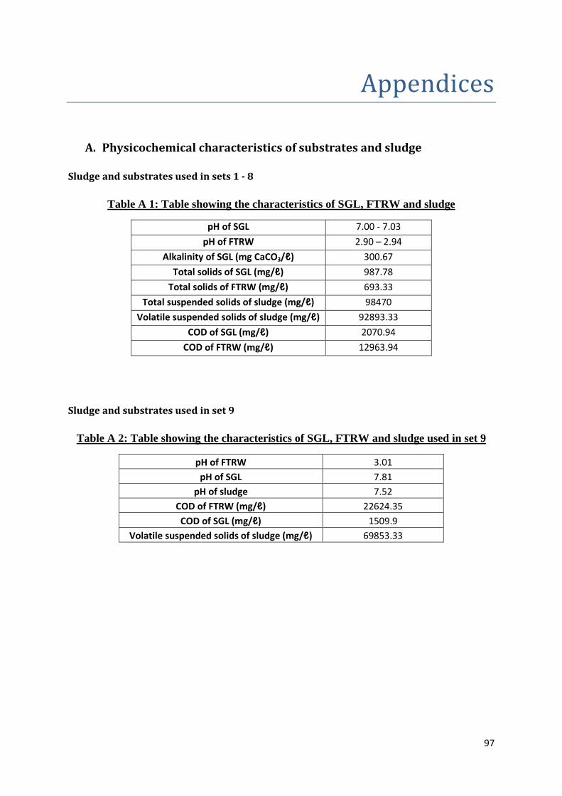
97

Appendices

A. Physicochemical characteristics of substrates and sludge

Sludge and substrates used in sets 1 - 8

Table A 1: Table showing the characteristics of SGL, FTRW and sludge

pH of SGL 7.00 - 7.03

pH of FTRW 2.90 – 2.94

Alkalinity of SGL (mg CaCO3/ℓ) 300.67

Total solids of SGL (mg/ℓ) 987.78

Total solids of FTRW (mg/ℓ) 693.33

Total suspended solids of sludge (mg/ℓ) 98470

Volatile suspended solids of sludge (mg/ℓ) 92893.33

COD of SGL (mg/ℓ) 2070.94

COD of FTRW (mg/ℓ) 12963.94

Sludge and substrates used in set 9

Table A 2: Table showing the characteristics of SGL, FTRW and sludge used in set 9

pH of FTRW 3.01

pH of SGL 7.81

pH of sludge 7.52

COD of FTRW (mg/ℓ) 22624.35

COD of SGL (mg/ℓ) 1509.9

Volatile suspended solids of sludge (mg/ℓ) 69853.33

98

B. Gas chromatograph calibration curves for biogas testing

Figure B 1: Graph showing the response of air (mV/s) when different volumes of air

(mℓ) are injected into a gas chromatograph

Figure B 2: Graph showing the response of nitrogen (mV/s) when different volumes of

nitrogen (mℓ) are injected into a gas chromatograph

y = 2E+06x R² = 0.9928

0

100000

200000

300000

400000

500000

600000

700000

800000

900000

1000000

0 0.1 0.2 0.3 0.4 0.5

Re

spo

nse

(u

V/m

in)

Volume of air (mℓ)

Air calibration

Upper 95% confidenceinterval

Lower 95% confidenceinterval

Linear (Air calibration)

y = 5E+06x R² = 0.9956

0

500000

1000000

1500000

2000000

2500000

0 0.1 0.2 0.3 0.4 0.5

Re

spo

nse

(u

V/m

in)

Volume of nitrogen (mℓ)

Nitrogen calibration



Linear (Nitrogen calibration)

99

Figure B 3: Graph showing the response of carbon dioxide (mV/s) when different

volumes of carbon dioxide (mℓ) are injected into a gas chromatograph

Figure B 4: Graph showing the response of methane (mV/s) when different volumes of

methane (mℓ) are injected into a gas chromatograph

y = 3E+06x R² = 0.9966

0

200000

400000

600000

800000

1000000

1200000

0 0.1 0.2 0.3 0.4 0.5

Re

spo

nse

(u

V/m

in)

Volume of carbon dioxide (mℓ)

Carbon dioxide calibration



Linear (Carbon dioxidecalibration)

y = 2E+06x R² = 0.9963

0

100000

200000

300000

400000

500000

600000

700000

800000

0 0.1 0.2 0.3 0.4 0.5

Re

spo

nse

(u

V/m

in)

Volume of methane (mℓ)

Methane calibration



Linear (Methanecalibration)

100

C. Proof of concept of water displacement method

Preparation of stock solution

Using acetate:

Molar mass = 60 g/mol

COD = 1.07 g COD/g acetate

Want a COD of 2.5 g/ℓ

for a 250 mℓ bottle:

(diluted in 5 mℓ water)

To make up a stock solution of 100 mℓ:

Using sodium acetate:

Molar mass of sodium = 82.03 g/mol

Molar mass of acetate = 60 g/mol

101

To make up a stock solution of 100 mℓ:

Theoretical amount of methane and carbon dioxide produced

0.584 g acetate is used per 250 mℓ bottle

For an ideal gas 1 mol = 22.4 ℓ

102

D. Volumes of sludge, nutrients and substrate used in experiments

Set 1: Testing the water displacement method with FTRW and UASB 1 sludge

Table D 1: Table showing the volumes of sludge, FTRW and nutrients used for set 1

FTRW:Sludge 0 0.2 0.25 0.3

Percentage sludge 25 25 25 25

Volume of sludge (mℓ) 75 75 75 75

mg VSS of sludge 1500 1500 1500 1500

mg COD of FTRW 0 300 375 450

Volume of FTRW (mℓ) 0 23.14 28.93 34.71

Volume of nutrients (mℓ) 75 75 75 75

Volume of liquid (mℓ) 150 173.14 178.93 184.71

Headspace (mℓ) 150 126.86 121.07 115.29

Headspace: total volume 0.5 0.42 0.40 0.38

Set 2: Testing the acidified brine solution displacement method


FTRW:Sludge 0 0.25 0 0.25



mg VSS of sludge 3000 3000 1800 1800

mg VSS/ℓ 20000 14433.29 10000 8383.34

mg COD of FTRW 0 750 0 450

Volume of FTRW (mℓ) 0 57.85 0 34.71

g COD/ℓ 0 3 0 1.8

Volume of nutrients (mℓ)

90 90

Volume of liquid (mℓ) 150 207.85 180 214.71

Headspace (mℓ) 150 92.15 120 85.29


103

Set 3: Testing the necessity of nutrients


FTRW: Sludge 0 0.25 0 0.25


Volume of sludge (mℓ) 48.44 48.44 48.44 48.44

mg VSS of sludge 4500 4500 4500 4500

mg VSS/ℓ 20000 20000 20000 20000

mg COD of FTRW 0 1125 0 1125

Volume of FTRW (mℓ) 0 86.78 0 86.78

g COD/ℓ 0 4.5 0 4.5

Volume of nutrients (mℓ)

48.44 48.44

Volume of water (mℓ) 176.56 89.78 128.11 41.34

Volume of liquid (mℓ) 225 225 225 225

Headspace (mℓ) 75 75 75 75


Set 4: Testing the acidified brine solution displacement method with FTRW and UASB 2

sludge

Table D 4: Table showing the volumes of sludge and FTRW used for set 4



mg VSS of sludge 6591 6591 6591 6591

mg VSS/ℓ 26364 26364 26364 26364

mg COD of FTRW 0 259.28 388.92 518.56

Volume of FTRW (mℓ) 0 20 30 40

g COD/ℓ 0 1.04 1.56 2.07

Volume of water (mℓ) 200 180 170 160




104

Set 5: Comparison of the acidified brine solution method to the alkaline solution method


Water displacement method Alkaline solution method

Percentage sludge 0.17 0.17 0.17 0.17


mg VSS of sludge 10517.08 10517.08 10517.08 10517.08

mg VSS/ℓ 42068.33 42068.33 42068.33 42068.33

mg COD of FTRW 0 343.12 0 343.12


g COD/ℓ 0 1.37 0 1.37




Headspace:total volume 0.17 0.17 0.17 0.17

Set 6: COD values of 1, 1.5 and 2 g COD/ℓ




mg VSS of sludge 10517.08 10517.08 10517.08 10517.08

mg VSS/ℓ 42068.33 42068.33 42068.33 42068.33

mg COD of FTRW 0 343.12 514.68 686.25


g COD/ℓ 0 1.37 2.06 2.74





105

Set 7: COD values of 1, 1.5 and 2 g COD/ℓ




mg VSS of sludge 21034.17 21034.17 21034.17 21034.17

mg VSS/ℓ 84136.67 84136.67 84136.67 84136.67

mg COD of FTRW 0 343.12 514.68 686.25


g COD/ℓ 0 1.37 2.06 2.74





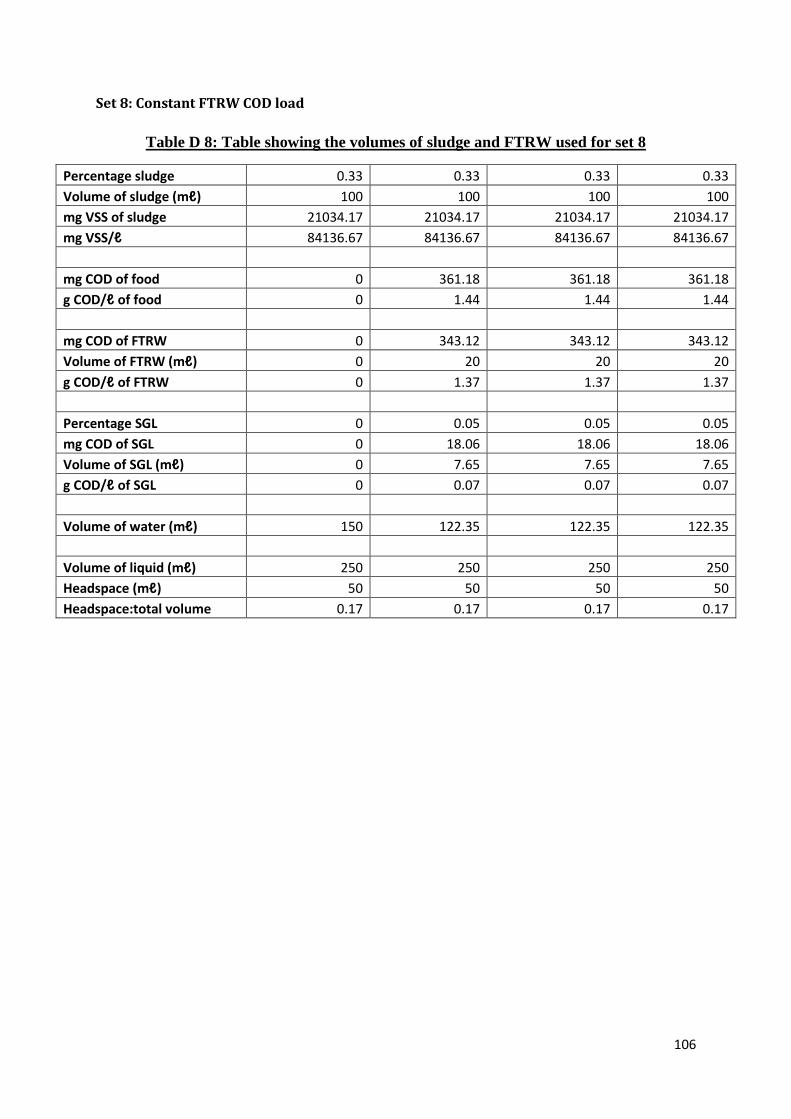
106

Set 8: Constant FTRW COD load




mg VSS of sludge 21034.17 21034.17 21034.17 21034.17

mg VSS/ℓ 84136.67 84136.67 84136.67 84136.67

mg COD of food 0 361.18 361.18 361.18

g COD/ℓ of food 0 1.44 1.44 1.44

mg COD of FTRW 0 343.12 343.12 343.12


g COD/ℓ of FTRW 0 1.37 1.37 1.37

Percentage SGL 0 0.05 0.05 0.05

mg COD of SGL 0 18.06 18.06 18.06

Volume of SGL (mℓ) 0 7.65 7.65 7.65

g COD/ℓ of SGL 0 0.07 0.07 0.07

Volume of water (mℓ) 150 122.35 122.35 122.35



Headspace:total volume 0.17 0.17 0.17 0.17

107

Set 9: Constant total COD load


Percentage sludge 0.17 0.17 0.17 0.17 0.17

Volume of sludge (mℓ) 50 50 50 50 50

mg VSS of sludge 1117.33 1117.33 1117.33 1117.33 1117.33

mg VSS/ℓ 4469.33 4469.33 4469.33 4469.33 4469.33

mg COD of food 0 257.39 257.39 257.39 257.39

g COD/ℓ of food 0 1.03 1.03 1.03 1.03

mg COD of FTRW 0 257.39 244.52 231.65 218.78

Volume of FTRW (mℓ) 0 8 7.6 7.2 6.8

g COD/ℓ of FTRW 0 1.03 0.98 0.93 0.88

Percentage SGL 0 0 0.05 0.1 0.15

mg COD of SGL 0 0 12.87 25.74 38.61

Volume of SGL (mℓ) 0 0 5.51 11.02 16.52

g COD/ℓ of SGL 0 0 0.05 0.1 0.15

Volume of water (mℓ) 200 192 186.89 181.78 176.68

Volume of liquid (mℓ) 250 250 250 250 250

Headspace (mℓ) 50 50 50 50 50

Headspace:total volume 0.17 0.17 0.17 0.17 0.17

108

E. Standard operating procedures

E1. Determination of characteristics of stripped gas liquor, Fischer-Tropsch reaction

water and UASB 1 sludge

pH test

Chemicals

Distilled water

Buffer solutions of pH 4.01, 7.01 and 10.01

Stripped gas liquor

Fischer-Tropsch reaction water

Equipment

Hanna pH meter (HI 255 combined meter) with pH probe (blue probe)

Temperature probe (silver probe)

Small beaker

Calibration procedure

1. The pH probe was washed with distilled water and wiped dry

2. The cal button on pH meter was pressed to begin calibration

3. The pH probe was placed in the buffer solution of the same pH as that displayed on

the right-hand side of the screen (eg. pH 7.01)

4. Waited until the reading was close to pH of buffer solution

5. When the screen displayed ready, the CFM/GLP button was pressed to confirm the

value

6. The pH probe was removed, washed with distilled water and wiped dry

7. The procedure was repeated for buffer solutions of pH 4.01 and 10.01 as prompted

pH measurement procedure

1. The pH and temperature probes were washed with distilled water and wiped dry

2. The beaker was washed with distilled water

3. A sample (i.e. stripped gas liquor or Fischer-Tropsch reaction water) was poured into

the beaker with a volume large enough for the tip of the pH probe to be completely

submerged

4. The pH and temperature probes were placed into the sample

5. The pH and temperature readings on pH meter were recorded when it became

relatively stable

109

6. The procedure was followed for three samples each for the stripped gas liquor and


7. The probes were washed and dried after each time it was placed into a solution

Alkalinity test

Chemicals

Distilled water

0.1 N sulphuric acid

Indicator: 0.2 g bromocresol green and 0.04 g methyl red in 100 mℓ 95% ethyl

alcohol

Stripped gas liquor

Equipment

Digital burette

Small beaker

Hanna pH meter with pH probe (blue probe)

25 mℓ volumetric flask

Alkalinity measurement procedure

1. The beaker and volumetric flask were washed with distilled water

2. The pH probe was washed with distilled water and dried

3. 25 mℓ of the stripped gas liquor was measured using the volumetric flask and poured

into the small beaker

4. Two drops of the indicator were added to the sample

5. The air bubbles in the digital burette were removed and the reading on the digital

burette was zeroed

6. The sample was titrated slowly and the pH was checked after every few drops of

sulphuric acid on the pH meter since the strip gas liquor was brown which made it

difficult to observe the colour change

7. The titration was continued and the pH checked until a pH of 4.5 was reached

8. The alkalinity was then calculated according the following equation:

(

)

110

Where:

A = Volume of sulphuric acid used (mℓ)

N = Normality of standard acid

V = Volume of sample (mℓ)

Table E 1: Table showing the alkalinity of SGL in mgCaCO3/ℓ

Sample Normality of acid

(N)

Volume of

sample (mℓ)

Volume of acid

used (mℓ)

Alkalinity

(mgCaCO3/ℓ)

SGL 1 0.1 25 1.51 302

SGL 2 0.1 25 1.51 302

SGL 3 0.1 25 1.49 298

Average 300.67

SD 2.31

%RSD 0.77

Sample calculation:

Total solids test

Chemicals

Distilled water

Stripped gas liquor


Equipment

Crucibles

Oven

Desiccator

Mass balance

Total solids measurement procedure

1. The crucibles were washed with distilled water

2. The crucibles were then placed in the oven at about 103 - 105°C for 2 hours to dry

3. Thereafter the crucibles were placed in the desiccator for 15 minutes to cool

111

4. Once cool, the crucibles were labelled (from 1 to 6) and weighed

5. 30 mℓ each of stripped gas liquor was added to the first three crucibles (1 to 3)

6. 30 mℓ each of Fischer-Tropsch reaction water was added to the other three crucibles

(4 to 6)

7. The crucibles were left in the oven overnight

8. The crucibles were then placed in the desiccator for 15 minutes to cool

9. The weight of the crucibles and the residue were measured

10. The total solids was calculated according to the following equation:

(

)

Where:

W1 = Weight of crucible (g)

W2 = Weight of crucible + residue (g)


Table E 2: Table showing the total solids (mg/ℓ) of SGL and FTRW

Sample Weight of

crucible only

(g)

Volume of

sample (mℓ)

Weight of

crucible +

residue (g)

Weight of

residue only

(g)

Total solids

(mg/ℓ)

SGL 1 30.8842 30 30.9124 0.0282 940

SGL 2 33.0619 30 33.0900 0.0281 936.7

SGL 3 27.0261 30 27.0587 0.0326 1086.7

Average 987.78

SD 85.66

%RSD 8.67

FTRW 1 29.7381 30 29.7621 0.0240 800

FTRW 2 30.1774 30 30.1950 0.0176 586.7

Average 693.33

SD 75.43

%RSD 10.88

Sample calculation:

112

Total suspended solids test

Chemicals

Distilled water

Stripped gas liquor


Equipment

Whatman glass microfiber filters (90 mm diameter)

Desiccator

Mass balance

Funnel and flask

Vacuum pump

Crucibles

Oven

Total suspended solids measurement procedure

1. The filter papers were placed in the oven at about 103 - 105°C for 30 minutes to dry

2. The filter papers were then placed in the desiccator for 20 minutes to cool

3. The filter papers were labelled, weighed and the weights were recorded

4. A filter paper was placed in the funnel and the vacuum pump was switched on

5. The filter paper was wet with distilled water to seal it to the funnel surface

6. 100 mℓ of the sample (Fischer-Tropsch reaction water or stripped gas liquor) was

poured into the funnel onto the middle of the filter paper

7. After filtration, the filter paper was removed, folded in half and placed into a labelled

crucible

8. The crucible was then placed into the oven at 103 - 105°C for 1 hour

9. This was done 3 times for the Fischer-Tropsch reaction water and 3 times for the

stripped gas liquor

10. Two blanks were prepared by using the same volume (100 mℓ) of distilled water as

the sample and following the above procedure

11. After 1 hour all of the crucibles were removed from the oven and placed into the

desiccator for 20 minutes to cool

12. The filter papers with the solid residue were weighed and the suspended solids was

calculated according to the following equation:

(

)

[ ]

113

Where:

W1 = Weight of filter paper (g)

W2 = Weight of filter paper + residue (g)

WB = Weight of blank (g)


Table E 3: Table showing the total, volatile and fixed suspended solids (mg/ℓ) of the

sludge

Sample Weight of

filter

paper

only (g)

Volume

of

sample

(mℓ)

Weight of

filter paper +

residue

before

ignition (g)

Weight of

filter paper +

residue after

ignition (g)

Total

suspended

solids

(mg/ℓ)

Volatile

solids

(mg/ℓ)

Fixed

solids

(mg/ℓ)

Sludge 1 0.3983 10 0.4664 0.4151 6810 5130 1680

Sludge 2 0.3909 10 1.0349 0.4517 64400 58320 6080

Sludge 3 0.3968 10 2.6388 0.4865 224200 215230 8970

Average 98470 92893.33 5576.67

SD 112628.49 109233.64 3670.97

%RSD 114.38 117.59 65.83

Sample calculation:

Volatile and fixed solids test

(Follows on from total suspended solids test)

Chemicals

As above

Equipment

Furnace

As above

114

Volatile and fixed solids measurement procedure

1. The filter paper and residue from total suspended solids test were placed into the

furnace at 550°C for 30 minutes to ignite to constant weight

2. After 1 hour, the samples were removed and cooled partially in air

3. The samples were then cooled in the desiccator

4. The filter papers and the residue were weighed and recorded

5. The volatile solids and fixed solids were calculated according to the following

equations:

(

)

(

)

Where:

W1 = Weight of filter paper (g)

W2 = Weight of filter paper + residue before ignition (g)

W3 = Weight of filter paper + residue after ignition (g)


Sample calculation (from Table E3):

Chemical oxygen demand test

Chemicals

Potassium dichromate (K2Cr2O7)

Silver sulphate (Ag2SO4)

Sulphuric acid (H2SO4)

1,10-Phenanthroline monohydrate (C12H8N2.H2O)

Ferrous sulphate heptahydrate (FeSO4.7H2O)

Ammonium iron (II) sulphate hexahydrate (Fe(NH4)2(SO4)2.6H2O)

Distilled water

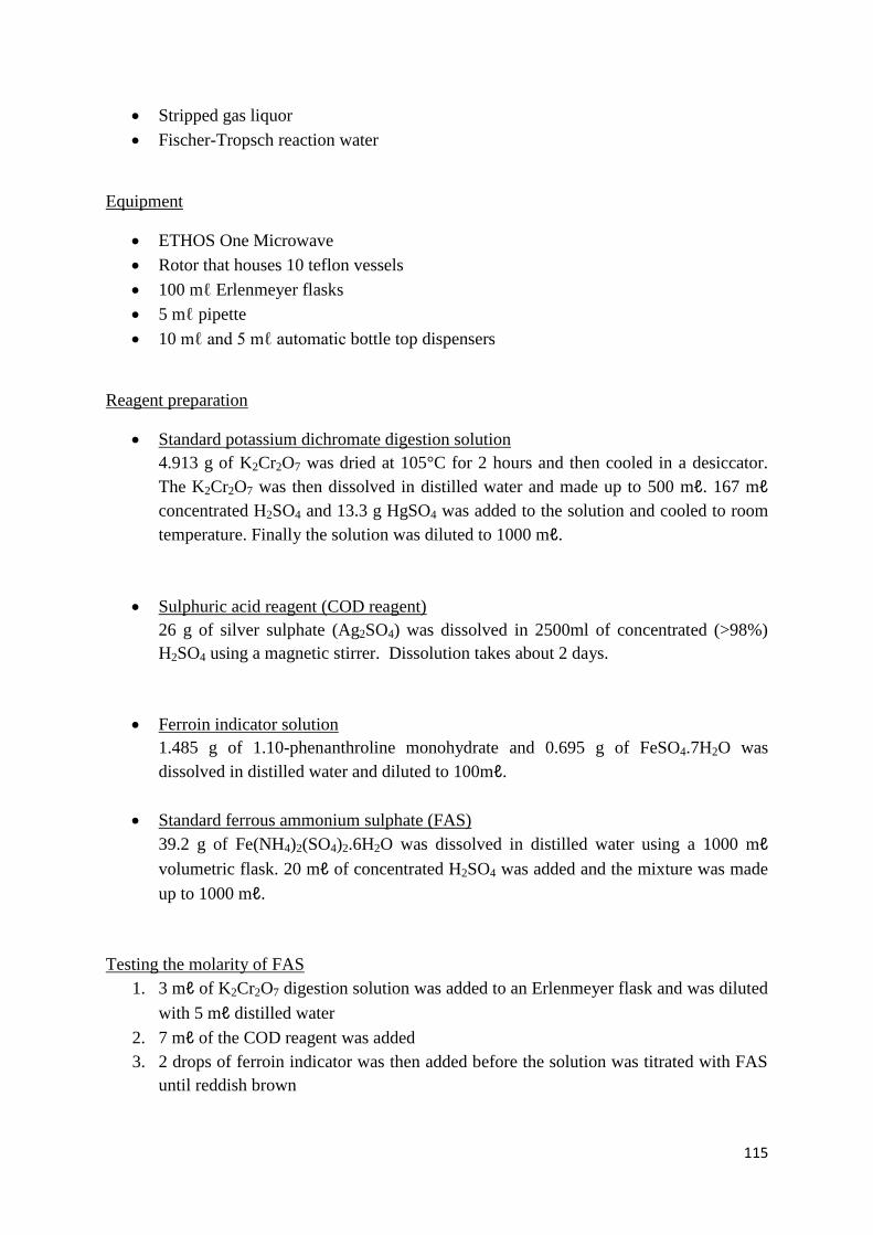
115

Stripped gas liquor


Equipment

ETHOS One Microwave

Rotor that houses 10 teflon vessels

100 mℓ Erlenmeyer flasks

5 mℓ pipette

10 mℓ and 5 mℓ automatic bottle top dispensers

Reagent preparation

Standard potassium dichromate digestion solution

4.913 g of K2Cr2O7 was dried at 105°C for 2 hours and then cooled in a desiccator.

The K2Cr2O7 was then dissolved in distilled water and made up to 500 mℓ. 167 mℓ

concentrated H2SO4 and 13.3 g HgSO4 was added to the solution and cooled to room

temperature. Finally the solution was diluted to 1000 mℓ.

Sulphuric acid reagent (COD reagent)

26 g of silver sulphate (Ag2SO4) was dissolved in 2500ml of concentrated (>98%)

H2SO4 using a magnetic stirrer. Dissolution takes about 2 days.

Ferroin indicator solution

1.485 g of 1.10-phenanthroline monohydrate and 0.695 g of FeSO4.7H2O was

dissolved in distilled water and diluted to 100mℓ.

Standard ferrous ammonium sulphate (FAS)

39.2 g of Fe(NH4)2(SO4)2.6H2O was dissolved in distilled water using a 1000 mℓ

volumetric flask. 20 mℓ of concentrated H2SO4 was added and the mixture was made

up to 1000 mℓ.

Testing the molarity of FAS

1. 3 mℓ of K2Cr2O7 digestion solution was added to an Erlenmeyer flask and was diluted

with 5 mℓ distilled water

2. 7 mℓ of the COD reagent was added

3. 2 drops of ferroin indicator was then added before the solution was titrated with FAS

until reddish brown

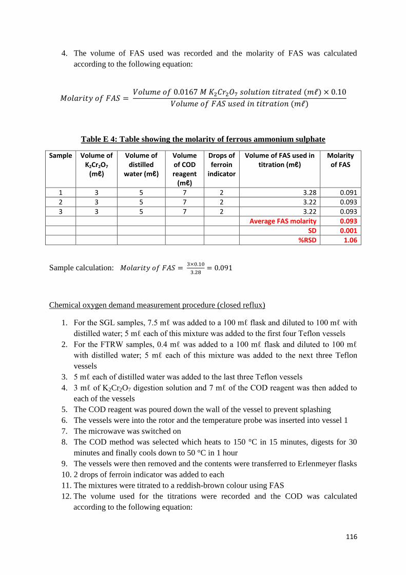
116

4. The volume of FAS used was recorded and the molarity of FAS was calculated

according to the following equation:

Table E 4: Table showing the molarity of ferrous ammonium sulphate

Sample Volume of K2Cr2O7

(mℓ)

Volume of distilled

water (mℓ)

Volume of COD reagent

(mℓ)

Drops of ferroin

indicator

Volume of FAS used in titration (mℓ)

Molarity of FAS

1 3 5 7 2 3.28 0.091

2 3 5 7 2 3.22 0.093

3 3 5 7 2 3.22 0.093

Average FAS molarity 0.093

SD 0.001

%RSD 1.06

Sample calculation:

Chemical oxygen demand measurement procedure (closed reflux)

1. For the SGL samples, 7.5 mℓ was added to a 100 mℓ flask and diluted to 100 mℓ with

distilled water; 5 mℓ each of this mixture was added to the first four Teflon vessels

2. For the FTRW samples, 0.4 mℓ was added to a 100 mℓ flask and diluted to 100 mℓ

with distilled water; 5 mℓ each of this mixture was added to the next three Teflon

vessels

3. 5 mℓ each of distilled water was added to the last three Teflon vessels

4. 3 mℓ of K2Cr2O7 digestion solution and 7 mℓ of the COD reagent was then added to

each of the vessels

5. The COD reagent was poured down the wall of the vessel to prevent splashing

6. The vessels were into the rotor and the temperature probe was inserted into vessel 1

7. The microwave was switched on

8. The COD method was selected which heats to 150 °C in 15 minutes, digests for 30

minutes and finally cools down to 50 °C in 1 hour

9. The vessels were then removed and the contents were transferred to Erlenmeyer flasks

10. 2 drops of ferroin indicator was added to each

11. The mixtures were titrated to a reddish-brown colour using FAS

12. The volume used for the titrations were recorded and the COD was calculated

according to the following equation:

117

(

) *

+

Where:

8000 = milliequivalent weight of O2 × 1000 mℓ/ℓ

Table E 5: Table showing the chemical oxygen demand (mgO2/ℓ) of SGL and FTRW

Sample Volume of sample (mℓ)

Volume of

K2Cr2O7 (mℓ)

Volume of COD

reagent (mℓ)

Drops of ferroin

indicator

Volume of FAS used in

titration (mℓ)

COD (mgO2/ℓ)

Blank 1 5 3 7 2 3.2

Blank 2 5 3 7 2 3.17

Blank 3 5 3 7 2 3.09

Average 3.15

SD 0.057

%RSD 1.80

SGL 1 5 (DF = 40/3) 3 7 2 2.03 2219.1

SGL 2 5 (DF = 40/3) 3 7 2 2.17 1942.53

SGL 3 5 (DF = 40/3) 3 7 2 2.07 2140.08

Average 2.15 1982.04

SD 2.11 2070.94

%RSD 0.066

3.14

FTRW 1 5 (DF = 250) 3 7 2 2.86 10865.02

FTRW 2 5 (DF = 250) 3 7 2 2.78 13828.21

FTRW 3 5 (DF = 250) 3 7 2 2.77 14198.61

Average 2.80 12963.94

SD 0.049

%RSD 1.76

Sample calculation: *

+

118

E2. Serum bottle test procedure

Serum bottle test procedure with water displacement method or acidified brine

solution method

Chemicals

Sludge

Stripped gas liquor


Water

Sodium chloride

Sulphuric acid

Apparatus

Water bath

Temperature regulator

Dropper stand

Twelve 250 mℓ serum bottles

Serum bottle metal holder

24 droppers

Procedure

1. Clamp droppers to stand (12 at the bottom – for gas collection and 12 at the top – for

water displacement)

2. Attach a pipe from the bottom dropper to the top dropper so that there are 12 pairs

3. Ensure that water bath is filled to the correct level and temperature regulator is at

35°C

4. Fill bottom droppers with water (or acidified brine solution)

5. The acidified brine solution is made up by adding sodium chloride to water until

supersaturated and then adding a few drops of sulphuric acid

6. Fill serum bottles with the appropriate volume of sludge, substrate (e.g. stripped gas

liquor and Fischer-Tropsch reaction water) and nutrients (if necessary)

7. Flush with nitrogen

8. Place serum bottles in metal holders in water bath

9. Attach pipe at the top of the gas collection dropper to serum bottle

10. Record volume of gas collected at regular intervals

11. Analyse gas composition using gas chromatograph

119

Serum bottle test procedure with alkaline solution method

Chemicals

Sludge

Stripped gas liquor


Distilled water

Sodium hydroxide

Apparatus

Water bath

Temperature regulator

Stand

Twenty-four 250 mℓ serum bottles

Serum bottle metal holder

Twelve 100 mℓ plastic cylinders

Procedure

1. Ensure that water bath is filled to the correct level and temperature regulator is at

35°C

2. Make up an alkaline solution by dissolving sodium hydroxide in distilled water

3. Fill twelve serum bottles with the alkaline solution

4. Fill the other twelve serum bottles with the appropriate volume of sludge, substrate

(e.g. stripped gas liquor and Fischer-Tropsch reaction water) and nutrients (if

necessary)

5. Place serum bottles in metal holders in water bath

6. Place the twelve plastic cylinders at the bottom of the stand

7. Use the pipes to connect the serum bottles in the water bath in which the reaction is

taking place to the serum bottles which are filled with the alkaline solution

8. Turn the bottles filled with the alkaline solution upside-down and attach to the stand

above the plastic cylinders

9. Record volume of alkaline solution collected (which is a direct indication of methane

collected) at regular intervals

120

E3. Gas chromatograph calibration and biogas testing

Chemicals

Helium

Nitrogen

Carbon dioxide

Methane

Equipment

Shimadzu gas chromatograph

Gas tight syringe

Switching on the gas chromatograph

1. The helium valve was opened

2. The gas chromatograph was switched on

3. The GC Real Time Analysis program and the Pollution_Research_Group method

were opened

Oven profile: 100 °C for 8 minutes

Carrier gas: constant flow He, 25 mℓ/min

Injection: 25 °C

Column: Carboxen, length = 1.5 m, I.D. = 2.1 mm

4. The column temperature was checked to ensure that it was set at 100°C

5. The system was switched on and left to reach the required temperature

6. Thereafter the detector was switched on and left until the baseline stabilised

Calibrating the gas chromatograph

1. The gases that were calibrated were air, nitrogen, methane and carbon dioxide

2. The gas being calibrated was collected in a gas collection unit (bomb)

3. The calibration was started with methane gas

4. The methane line was connected to the gas collection unit, both valves on the unit

were opened and the unit was flushed with methane for approximately 3 minutes

5. Both the valves were then closed

6. The button Single Run was clicked on and a file was opened to save the results by

clicking on Sample Login

7. It was ensured that the program indicated that the gas chromatograph was ready and

then the start button on the program was pressed

121

8. 0.1 mℓ of methane was then injected into the gas chromatograph and the start button

on the gas chromatograph was pushed

9. When the analysis was complete the stop button on the program was pressed

10. The analyses were done for four different volumes i.e. 0.1, 0.2, 0.3 and 0.4 mℓ and

each volume done in triplicates

11. The response (area) obtained was plotted against the volume in Microsoft Excel

12. The procedure was repeated for air, nitrogen and carbon dioxide

Gas testing

1. A sample of 0.4 mℓ was obtained from each bottle and injected into the gas

chromatograph following the procedure above

2. Each run takes about 7-8 minutes to complete

Switching off the gas chromatograph

1. The system was switched off and left to cool for about 30 minutes

2. The detector was then switched off and the program was closed

3. The gas chromatograph was switched off and the helium valve was closed

E4. Phenol measurement

Colorimetric method

Chemicals

Ammonium chloride (NH4Cl)

Ammonium hydroxide (NH4OH)

Distilled water

4-aminoantipyrine

Potassium ferricyanide (K3Fe(CN)6)

Phenol

Stripped gas liquor


Equipment

100 mℓ volumetric flasks

Erlenmeyer flasks

pH meter

122

1-10 mℓ pipette

10-100µℓ pipette

Spectrometer

Reagent preparation

Buffer solution

16.9 g of ammonium chloride was dissolved in 143 mℓ of ammonium hydroxide and

thereafter diluted to 250 mℓ with distilled water.

Aminoantipyrine solution

2 g of 4-aminoantipyrine was added to a 100 mℓ volumetric flask and diluted to 100

mℓ with distilled water.

Potassium ferricyanide solution

8 g of potassium ferricyanide was added to a 100 mℓ volumetric flask and diluted to

100 mℓ with distilled water.

Stock phenol solution

1 g of phenol was added to a 1 ℓ volumetric flask and diluted to 1 ℓ with distilled

water

Standard addition method

1. Five 100 mℓ volumetric flasks were washed

2. 0, 0.2, 0.4, 0.6 and 0.8 mℓ (later modified to 0, 0.02, 0.04, 0.06 and 0.08 mℓ) of the

1000 mg/ℓ stock phenol solution was added to each of the flasks respectively

3. 10 mℓ of the sample was added to each flask and mixed

4. These were diluted to 100 mℓ with distilled water

5. 2 mℓ of the buffer solution was added to each flask and mixed to increase the pH of

the solution

6. The pH of the solutions with the lowest (0 mg/ℓ) and highest concentrations (0.8

mg/ℓ) were determined with the pH meter to ensure that they were above a pH of 10

7. 2 mℓ of the aminoantipyrine solution was added to each of the flasks and mixed

8. Finally 2 mℓ of the potassium ferricyanide solution was added to each of the flasks

and mixed

9. This gave a total volume of 106 mℓ, therefore giving a dilution factor of 10.6

10. The solutions were then allowed to stand for 15 minutes and thereafter the absorbance

was measured with the spectrometer at 510 nm

11. Three readings were taken for each sample

12. The absorbance was plotted against the concentration

13. The graph was extrapolated until it intercepted the x-axis

123

14. The concentration of the phenols in the sample was calculated by multiplying the

dilution factor and the x-intercept

Figure E 1: Graph showing the extrapolated graph of the absorbance (λ) of light of the

solution at a wavelength of 510 nm against the phenol concentration of the standard

solutions

Phenol concentration of the sample = |x-intercept| × dilution factor

= (-0.07/0.1143) × (106/10)

= 0.61 × 10.6

= 6.49 mg/ℓ

Gas Chromatography

Solid phase extraction

Chemicals

Dichloromethane

Hexane

Phenol

Stripped gas liquor

y = 0.1143x + 0.07 R² = 0.9955

-0.02

0

0.02

0.04

0.06

0.08

0.1

0.12

0.14

0.16

0.18

-1 -0.5 0 0.5 1Ab

sorb

ance

(λ)

at

wav

elen

gth

of

51

0 n

m

Phenol concentration (mg/ℓ)

Series1

Series2

Series3

Average

Linear (Average)

124

Equipment

SPE vacuum

200 mg Strata Silica cartridges from Phenomenex

Vacuum pump

Two beakers for hexane and dichloromethane

Beakers for samples

Glass vials

Pipette to measure out hexane, dichloromethane and samples

15 ml Cellstar tubes

Solid phase extraction procedure

1. Remove top of SPE vacuum and place glass vials (without the caps) in the SPE

vacuum manifold

2. Replace top and ensure that the droppers fit into the glass vials and top fits securely

3. Remove yellow caps from the SPE vacuum and attach cartridges

4. Attach the vacuum pump to the SPE vacuum

5. Open SPE vacuum valves

6. Condition/equilibrate cartridges by adding 1 ml of dichloromethane to each cartridge

and turn on vacuum slowly

7. Turn off vacuum after dichloromethane has passed through the cartridges

8. Condition/equilibrate cartridges by adding 1 ml of hexane to each cartridge and turn

on vacuum slowly

9. Turn off vacuum after hexane has passed through the cartridges

10. Add 7 ml of sample (phenol or stripped gas liquor) to the cellstar tube, followed by 7

ml of hexane and shake thoroughly

11. Add 2 ml of this mixture to each cartridge (take sample from bottom of cellstar tube)

12. Turn on the vacuum slowly

13. Turn off vacuum after sample has passed through the cartridges

14. Wash cartridges by adding 1 ml of hexane to each cartridge and turn on vacuum

slowly

15. Turn off vacuum after hexane has passed through the cartridges

16. Wash once more with 1 ml of hexane

17. Increase vacuum to just below 20 inches of mercury and leave for approximately 10

minutes to dry cartridges

18. Turn off vacuum and close SPE vacuum valves

19. Remove top of SPE vacuum remove glass vials (waste) and place new clean glass

vials, without the caps, (cleaned with dichloromethane) in the SPE vacuum manifold

20. Replace top and ensure that the droppers fit into the glass vials and top fits securely

21. Open SPE vacuum valves

22. Elute by adding 1 ml of dichloromethane to each cartridge and turn on the vacuum

slowly

125

23. Turn off vacuum after dichloromethane has passed through the cartridges

24. Elute once more with 1 ml of dichloromethane

25. Turn off vacuum and close SPE vacuum valves

26. Remove cartridges and throw away

27. Replace yellow caps

28. Remove top of SPE vacuum, remove glass vials with samples and replace caps

(ensure that glass vials are labelled appropriately so as to not confuse samples)

29. Replace top and ensure that it fits securely

30. Remove vacuum pump

GC

Chemicals

Acetone

Sample prepared using solid phase extraction

Helium

Hydrogen

Air

Equipment

Shimadzu GC2010 Plus

Glass vial

Switching on the GC

1. The helium, hydrogen and air valves were opened

2. The gas chromatograph was switched on

3. The computer was switched on and the GC Solution program was opened

4. The method, ReneMethod2, was opened:

Oven profile: 60 °C to 240 °C at 20 °C/min for 6 minutes

Carrier gas: constant flow He, 0.23 mℓ/min

Injection: 220 °C

Column: ZB-WAXplus, length = 30 m, I.D. = 0.25 mm

5. The system was switched on and the parameters were downloaded

6. The GC was left to reach the required temperature and stabilise

7. When the GC had reached the required parameters “Ready” was displayed on the

screen

8. Before performing any runs ensure that the solvent vial is full

126

Calibrating the GC

1. Different concentrations of phenol were prepared using the solid phase extraction

2. The first (lowest) concentration of phenol was emptied into the 1.5mℓ vial and placed

in the sample rack

3. The sample was logged in by clicking on Sample Login on the side-bar and a name

for the file was entered

4. The run was then started by clicking on Start on the side-bar

5. The run takes 15 minutes to complete (phenol elutes at approximately 2.4 minutes)

6. The same sample was repeated 2 more times

7. The first concentration was removed, the next concentration was placed in the sample

rack and the procedure was repeated

8. This was done for all concentrations of phenol

9. The file of the completed run was opened and the peak at 2.4 minutes was integrated

10. The retention time, area and height of the peak were recorded

11. The phenol concentration was then plotted against the area and the height on

Microsoft Excel to obtain the calibration curve

Sample testing

1. The sample was emptied into the 1.5mℓ vial and placed in the sample rack

2. The sample was logged in by clicking on Sample Login on the side-bar and a name

for the file was entered

3. The run was then started by clicking on Start on the side-bar

4. The run takes 15 minutes to complete (phenol elutes at approximately 2.4 minutes)

5. The same sample was repeated 2 more times

6. The file of the completed run was opened and the peak at 2.4 minutes was integrated

7. The retention time, area and height of the peak were recorded

8. Using the area of the peak of the sample and the calibration curve, the phenol

concentration of the sample was determined

Switching off the GC

1. The system was switched off and left to cool down

2. The GC was then switched off

3. The helium, hydrogen and air valves were closed

127

F. Paired two sample t-test

The paired t-test examines if the difference between the means is significantly different

from the hypothesised value of zero, = 0 (Park, 2009). Microsoft Excel was used

to execute the t-test to compare the two sets of data. The analysis tool t-Test: Paired Two

Sample for Means was accessed under Data Analysis. The range of SMA values for the

test and reference units were selected and an alpha value of 0.05 was used. A table

presenting the P-value was displayed. For example, for the comparison of the 5% SGL

test unit SMA and the paired reference unit SMA in set 8, the following table was

obtained:

Table F 1: Table showing the results from the paired two sample t-test

Variable 1 Variable 2

Mean 0.598095292 0.476312

Variance 0.210954727 0.067458

Observations 10 10

Pearson Correlation 0.832777063

Hypothesized Mean Difference 0

df 9

t Stat 1.363916232

P(T<=t) one-tail 0.102864051

t Critical one-tail 1.833112933

P(T<=t) two-tail 0.205728102

t Critical two-tail 2.262157163

Therefore P = 0.103

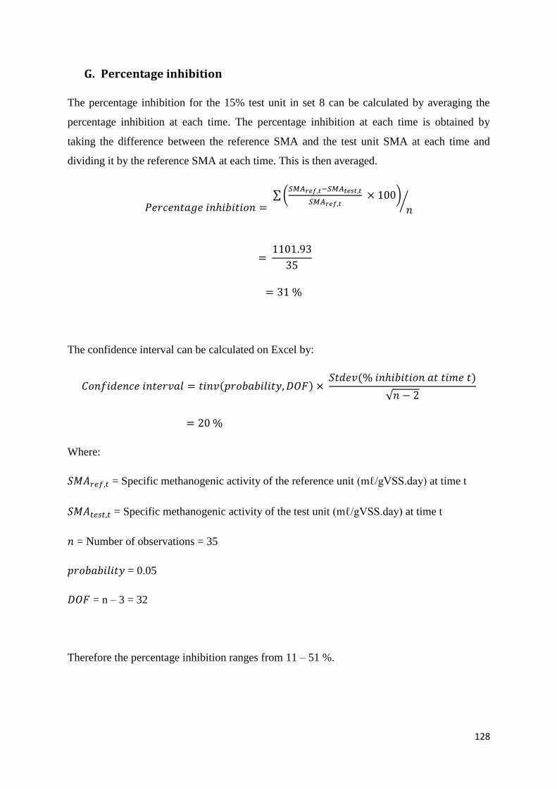
128

G. Percentage inhibition

The percentage inhibition for the 15% test unit in set 8 can be calculated by averaging the

percentage inhibition at each time. The percentage inhibition at each time is obtained by

taking the difference between the reference SMA and the test unit SMA at each time and

dividing it by the reference SMA at each time. This is then averaged.

∑ (

)

⁄

The confidence interval can be calculated on Excel by:

√

Where:

= Specific methanogenic activity of the reference unit (mℓ/gVSS.day) at time t

= Specific methanogenic activity of the test unit (mℓ/gVSS.day) at time t

= Number of observations = 35

= 0.05

= n – 3 = 32

Therefore the percentage inhibition ranges from 11 – 51 %.

129

An alternative way to calculate the percentage inhibition for the 15% test unit in set 8 is by

comparing the average SMA difference to the average reference SMA. The SMA difference

is obtained by taking the difference between the reference SMA and the test unit SMA at

each time. These values are then averaged to get the average SMA difference.

∑ ⁄

∑ ⁄

⁄

⁄

This value fits into the range calculated above.

The percentage inhibition can also be calculated by comparing the cumulative methane

produced in the test unit from day 2 to day 9 to the cumulative methane produced in the

reference unit.

(

)

(

)

This value also falls between the range above.

130

Figure G 1: Graph showing the cumulative net methane produced (mℓ) over time (days)

for the 15% SGL test unit in set 8 and the matching reference test

0

5

10

15

20

25

30

0 2 4 6 8 10

Cu

mu

lati

ve n

et

me

than

e v

olu

me

(m

ℓ)

Time (days)


1 g COD/ℓ FTRW

Investigation into the effect of stripped gas liquor on ...

Documents

Transcript of Investigation into the effect of stripped gas liquor on ...