
Investigation into skill leveled operators in a multi ...
14
Transcript of Investigation into skill leveled operators in a multi ...
Scientia Iranica E (2020) 27(6), 3219{3232
Sharif University of TechnologyScientia Iranica
Transactions E: Industrial Engineeringhttp://scientiairanica.sharif.edu
Investigation into skill leveled operators in amulti-period cellular manufacturing system with theexistence of multi-functional machines
M. Ra�ee� and A. Mohamaditalab
Department of Industrial Engineering, Sharif University of Technology, Tehran, Iran.
Received 3 June 2017; received in revised form 3 July 2018; accepted 21 July 2019
KEYWORDSMulti-period cellularmanufacturingsystem;Machine reliability;Workforce learning-forgetting e�ect;Alternative processrouting.
Abstract. Numerous studies published in the �eld of cellular manufacturing system arebased on the assumption that machines are reliable in the entire production line withoutany breakdown. Since such assumptions are not usually realistic, to contribute to closingthis gap between assumption and reality, a new model was proposed that additionallyconsidered machine reliability, alternative process routings, and workforce assignment in adynamic environment. Given such considerations in this research, the modi�ed problem wasde�ned and formulated and an extended mixed integer multi-period mathematical modelwas proposed. In order to evaluate the e�ectiveness and capability of the extended model,some hypothetical numerical instances were generated and computational experiments werecarried out using GAMS optimization package. Experimental results demonstrated thatthe demand value could a�ect the machine breakdown rate, and a machine with a minimumbreakdown rate was implemented more often than others. Moreover, the observed trade-o� between the workforce-related costs and cell-formation costs indicated that workforce-related issues had a signi�cant impact on the total e�ciency of the system. The proposedmodel can be quite applicable to medium- and large-scale manufacturing companies.© 2020 Sharif University of Technology. All rights reserved.
1. Introduction
Group Technology (GT), known as an e�ective manu-facturing technique, necessitates, as the name suggests,ful�lling similar tasks in the same way. This approachcan be viably employed in a competitive production en-vironment, which makes manufacturing systems adaptthemselves to the erratic changes and dynamics ofproduction factors such as part demand changes, newproduct development, machine requirements, etc. Be-ing highly potential and enjoying high performance in
*. Corresponding author. Tel.: +98 21 6616 5725E-mail addresses: ra�[email protected] (M. Ra�ee);[email protected] (A. Mohamaditalab)
doi: 10.24200/sci.2019.21513
manufacturing, Cellular Manufacturing System (CMS)as an application of GT can be implemented at mostindustrial plants. However, Cell Formation (CF),Inter/intra-Cell Layout (CL), and workforce alloca-tion are the three main sub-problems in designingan e�cient CMS. Many researcher have tackled theseproblems e�ectively, especially in case of complicatedmodels, in which two or three of the abovementionedproblems are simultaneously taken into account. Liuet al. [1], for instance, presented a new model byintegrating production planning with facility transferin a dynamic cellular manufacturing environment inthe supply chain. Similarly, Askin [2] reviewed thedevelopment of CMS-related organizational issues andoptions. Accordingly, relevant studies can be catego-rized in terms of designing and optimization. Amongother studies, Ameli and Arkat [3] aimed to solve the
3220 M. Ra�ee and A. Mohamaditalab/Scientia Iranica, Transactions E: Industrial Engineering 27 (2020) 3219{3232
CF problem and developed a pure integer mathemat-ical model. They also considered issues of machinereliability and Alternative Process Routings (APRs).Bulgak and Bektas [4] conducted another research inwhich CF problem along with Production Planningwas investigated, and recon�guring the system wassimultaneously taken into consideration. Mehdizadehet al. [5] presented a multi-objective Mixed IntegerProgramming (MIP) model to simultaneously solve CFand production planning problems. They considerednumerous real-world parameters such as alternativeplans for processing the part types, exibility of work-ers and machines, multi-period production planning,capacity of machines, recon�guration of dynamic sys-tems, sequence of operations, duplicate machines, timeavailability of workers, and worker assignment weretaken into consideration. Furthermore, Mahdavi et al.[6] extended a dynamic CF considering PP and work-force assignment which aimed to minimize the currentinventory, in-process inventory and backlog, inter-cellpart trip, recon�guration of machines, and workforce-related costs. Similarly, Aryanezhad et al. [7] proposedan extended model to address CF and workforce as-signment problems while, at the same time, examiningthe following real-world production factors: exibilityof part routings, machine, and labor enhancementtraining for mastery of higher skill level. Similarly,Bagheri and Bashiri [8] proposed a comprehensivemodel in which the dynamic CF problems, includinginter-cell layout and workforce assignment problems,were integrated. In fact, in a dynamic environment,they analyzed the learning ability of labors. Javadi etal. [9] introduced a novel model in order to investigatethe layout and CF problems simultaneously. Theirproposed model attempted to design the material-handling ow path structure and inter/intra-cell layoutproblem concurrently. Bagheri et al. [10] considered anewfangled model for CMS considering some produc-toin features comprising reliability of machines withstochastic parameters such as service and arrival timesin a dynamic area and APRs. Moreover, they em-ployed a benders decomposition method to overcomethe complexity of the mentioned problem. Bayramand S�ahin [11] also proposed a mathematical modelin which many real-world production factors such assequences of operations, splitting of lots, changingdemands for products, capacities of machines, theproducts' alternative processing routes, and machineduplication were addressed.
Nowadays, in competitive production systems,the workforce-related issues are of importance. There-fore, it is necessary to review the relevant studies inthis domain. Recently, Azadeh et al. [12] applieda novel model to the dynamic CMS in a multi-objective area called MDCMS with emphasis on humanfactors. Two main objectives including minimizing
the inconsistency of the decision-making mode forthe workforce in the public manufacturing cells andbalancing the workload of the cells with respect toworkforce e�cacy were emphasized in their research.Moreover, in their research, Liu et al. [13] aimedto develop a combined decision model of productionplanning and assignment of workers in a dynamic CMSarea of �ber connector manufacturing business. In thesame manner, Mehdizadeh and Rahimi [14] attemptedto develop a joint model to tackle the dynamic CFproblem with emphasis on the assignment of workforceand inter/intra cell layout problems in the presence ofmachine duplication. Similarly, Ra�ei and Ghodsi [15]proposed an ant colony optimization to tackle theproblem of CF integrated with workforce-related issues.Sakhaii et al. [16] also proposed and applied robustoptimization methods to investigate the dynamic CFproblem with focus on the concepts of reliability ofmachines, production planning, allocation of workforce,inter cell layout, and APRs. A comprehensive multi-objective model of the CMS in a dynamic area wasextended by Nouri [17] who considered several keycell design factors including designations of machines,inter/intra-cell material handling, allotting of workers,workload balancing and outsourcing according to theoperation time, and the operation sequence of parts.However, in this study and other related researches,workforce-related issues were not addressed in detail.In addition, the present study aimed to �ll the gapmentioned earlier.
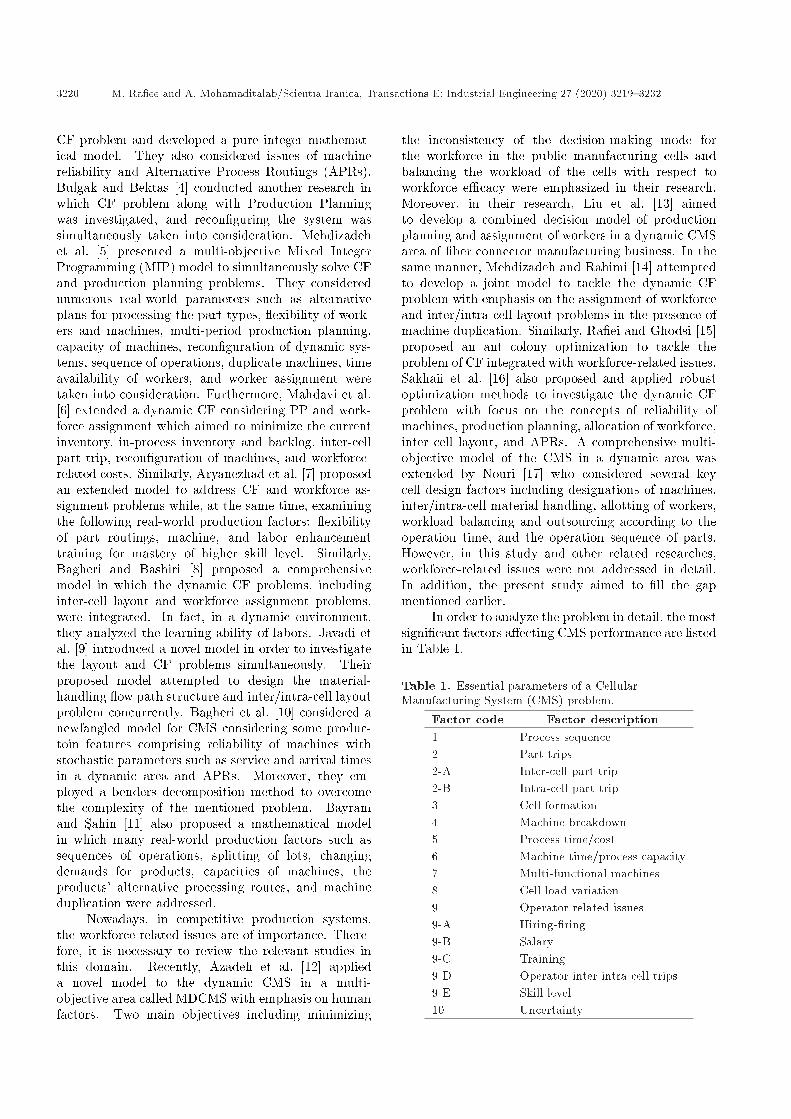
In order to analyze the problem in detail, the mostsigni�cant factors a�ecting CMS performance are listedin Table 1.
Table 1. Essential parameters of a CellularManufacturing System (CMS) problem.
Factor code Factor description1 Process sequence2 Part trips2-A Inter-cell part trip2-B Intra-cell part trip3 Cell formation4 Machine breakdown5 Process time/cost6 Machine time/process capacity7 Multi-functional machines8 Cell load variation9 Operator related issues9-A Hiring-�ring9-B Salary9-C Training9-D Operator inter-intra cell trips9-E Skill level10 Uncertainty

M. Ra�ee and A. Mohamaditalab/Scientia Iranica, Transactions E: Industrial Engineering 27 (2020) 3219{3232 3221
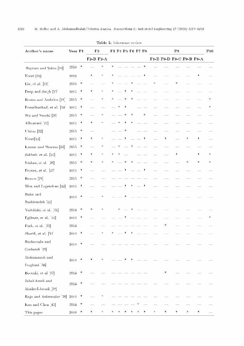
Based on the factors listed in Table 1, it has beenattempted to analyze the recent studies, the obtainedresults of which are reported in Table 2. According tothis table, several vital realistic assumptions such asreliability of machines, APRs, and workforce learning-forgetting e�ect have been neglected by a numberof previous studies. In the following, however, anoptimization problem will be introduced and general-ized by emphasizing the APRs and workforce-relatedissues while multi-functional machines are availableand machines are not reliable. The generalized problemis presented with the aim of reducing the inter-cellpart trips and minimizing machine breakdown andworkforce-related costs. In fact, the proposed modelis an extended version of the research conducted byBagheri and Bashiri [8], to which many other realisticfactors such as APRs, machine reliability, and work-force learning-forgetting e�ect are added.
In the following, a Mixed Integer Non-LinearMathematical Programming (MINLP) model will beproposed which is in line with the mentioned objectives.Then, a linearization technique was implemented toconvert the model into an MIP form. Section 3analyzes the e�ectiveness of the presented model whichis veri�ed through giving some numerical examplesfollowed by the conclusion and some suggestions forfuture research in the last section.
2. The optimization model
2.1. Problem explanation and mathematicalformulation
A majority of the previous approaches are based onan unrealistic assumption that machines are reliablein the whole production horizon without any break-down. In fact, in industrial environments, machinesare unreliable and their breakdown costs should beconsidered in order to enhance the e�ciency of CMS.To this end, this paper proposes a framework toconsider the costs of machine breakdown, i.e., repairingand installation-uninstallation costs. Consequently,exponential distribution should be considered with agiven breakdown (failure) rate of machine reliability inits operating time:R = exp(��t); (1)
where R is the machine reliability at time t. Thebreakdown rate � is also given in the planning horizon;therefore, the mean time among the failures calledMTBF is determined through Eq. (2):
MTBF =1�: (2)
To determine the total machine breakdown cost withinits production horizon, the total production time isdivided by its MTBF and then, the obtained value ismultiplied by machine-failure unit cost.
Other basic assumptions considered in modelingthe problem are described as follows:
1. Some features are already given and �xed overthe planning horizon such as the number of cells,demand of each part type in each period, andlower/upper bounds of cell capacity;
2. There are machine tools that can be installed onthe prede�ned machines. Each tool can be used tomachine a speci�c operation of a part;
3. Workforce can be assigned to the responsibility ofmore than one tool or machine according to theirskill level;
4. Training the operators is allowed; in other words,workforce could be taught to work with a particularmachine by paying a teaching cost. However, thetrained workforce can be applied in other periodswithout any extra training cost. Besides, accordingto a prede�ned forgetting rate, workforce mayforget working with a tool.
2.2. NotationsIndices:m The number of machines, m0 = 1; :::;Mg Machine tools, g0 = 1; :::; Gi = 1; :::; I The number of partsc The number of machine cells that
should be constructed, c0 = 1; :::; Cj = 1; :::; O The number of operations for each part
typet = 1; :::; T The number of manufacturing cycles
(term)k = 1; :::;K The number of available workforcel = 1; :::; L Workforce skill level
Input parameters:MCi Inter-cell part trip costSM Machine install/uninstall cost in a cellSG Tool install/uninstall cost on a machineijg Tool consumption costBm The repairing cost of machine \m"mcaptimem The maximum time of processing by
machine \m"um; lm The maximum and minimum numbers
of tools that can be installed onmachine \m"
uc; lc The maximum and minimum numbersof machines that could be assigned tocell \c"
q The percentage of cell load variation
MTBF =1�m
The average time of the machine \m"breakdowns
3222 M. Ra�ee and A. Mohamaditalab/Scientia Iranica, Transactions E: Industrial Engineering 27 (2020) 3219{3232
Table 2. Literature review
Author's name Year F1 F2 F3 F4 F5 F6 F7 F8 F9 F10
F2-B F2-A F9-E F9-D F9-C F9-B F9-A
Bayram and S�ahin [10] 2016 * { * * { { { { * { { { { { {
Nouri [16] 2016 * * * { { { { * { { { { * {
Liu, et al. [12] 2016 * { { * { { * { { * { * { { {
Deep and Singh [17] 2015 * * * * { * * { { { { { { { {
Renna and Ambrico [18] 2015 * { * * { * * { { { { { { { *
Esmailnezhad, et al. [19] 2015 * { { { * * { { { { { { { *
Wu and Suzuki [20] 2015 * { * { { * * * { { { { { {
Alhourani [21] 2015 * * * { * * * { { { { { { { {
Ulutas [22] 2015 * { { { * { { { { { { { {
Nouri[23] 2015 * * * { { * { { * { * { * * {
Kumar and Sharma [24] 2015 * { * { * { * { { { { { { { {
Sakhaii, et al. [25] 2015 * * * * * { { { { { * * *
Niakan, et al. [26] 2015 * * * * { * * { { { { { * * *
Erozan, et al. [27] 2015 * { { { { * { { * { { { { { {
Brusco [28] 2015 * { { { { { { { { { { { { { {
Won and Logendran [29] 2015 * { { { { * * { * { { { { { {
Halat and
Bashirzadeh [30]2015 * { * { { * { { { { { { { { {
Yadollahi, et al. [31] 2014 * * * * { * { { { { { { { {
Egilmez, et al. [32] 2014 * { { { { * { { { { { { { { *
Park, et al. [33] 2014 { { { { { { { { { * { { { {
Shari�, et al. [34] 2014 * { * * { * * { { { { { { { {
Baykasoglu and
Gorkemli [35]2014 * { { { { { { { { { { { { { {
Mohammadi and
Forghani [36]2014 * * * { { * * { { { { { { { {
Bootaki, et al [37] 2014 * { { { { { { { { * { { { {
Jabal-Ameli and
Moshref-Javadi [28]2014 * { { { { { { { { { { { { { {
Raja and Anbumalar [39] 2014 * { * { { { { { { { { { { { {
Kao and Chen [40] 2014 * { { { { { { * { { { { { { {
This paper 2016 * * * * * * * * * * * * * * {

M. Ra�ee and A. Mohamaditalab/Scientia Iranica, Transactions E: Industrial Engineering 27 (2020) 3219{3232 3223
H;F Workforce hiring/�ring costSAl The salary of the workforce with the
skill level lmovek The workforce trip cost of cellsat=1kg 1 if workforce k can work with tool g
at the start time of planning horizonawg The minimum skill level to work with
tool \g"@l Skill level boundaryw1; w2 Increase and decrease in workforce skill
levelDti The demand value for the i-th part in
the t-th manufacturing termdiscc0 The distance between the two
candidate locations c and c0timeijgm The processing time of operation j on
machine type m for part type i withtool g
MINEM The least number of workforce su�cientto be hired in each manufacturing term
Opcaptime The maximum time of working foreach workforce
�tijg 1 if operation j of part type i canbe processed by tool g in productionperiod t; 0 otherwise
�tgm 1 if tool g can be installed on machinem in production period t; 0 otherwise
Decision variables:
xtmc =
8><>:1; If machine m in period t is designatedto cell c
0; Otherwise
ytgm =
8><>:1; If tool g in period h is installedon machine m
0; Otherwise
ptijg =
8><>:1; If operation j of part type i in period tis processed with tool g
0; Otherwise
btk =
(1; If operator k is working in period t0; Otherwise
htk =
(1; If operator k is hired in period t0; Otherwise
wtkg =
8><>:1; If operator k is working with machinetool g in period t
0; Otherwise
letkl =
8><>:1; If operator k is in skill level of lin period t
0; Otherwise
at�2kg =
8><>:1; Ifoperator k can work with toolg in period t
0; Otherwise
2.3. The objective functionThe proposed MINLP model for the CMS design iso�ered as Eqs. (3) to (11):
min Model 1 :
TXt=1
IXi=1
OiXj=1
GXg;g0=1
MXm;m0=1
Xc;c6=c0
xtmc�ytgm�ptijg�xtm0c0
�ytg0m0�pti(j+1)g0�Dti�disc;c0�MCi; (3)
+TXt=1
IXi=1
OiXj=1
GXg;g0=1
CXc=1
Xm;m0 6=m
xtmc� ytgm� ptijg
� xtm0c� ytg0m0� pti(j+1)g0�Dti�MCi; (4)
+T�1Xt=1
MXm=1
Xc;c 6=c0
xtmc � xt+1mc0 � disc;c0 � SM; (5)
+TXt=1
MXm=1
IXi=1
OiXj=1
GXg=1
ytgm � ptijg �Dti �ijg; (6)
+T�1Xt=1
GXg=1
Xm;m 6=m0
ytgm � yt+1gm0 � SG; (7)
+TXt=1
MXm=1
IPi=1
OiPj=1
GPg=1
ptijg�ytgm�timeijgm�Dti
MTBFm
�Bm; (8)
KXk=1
(h1k�H)+
TXt=2
KXk=1
(htk�H+(1�btk)�F); (9)
+TXt=1
KXk=1
Xg;g0
Xm;m0
Xc;c 6=c0
wtkg � wtkg0 � ytgm � xtmc
� ytg0m0 � xtm0c0 � disc;c0 �movek; (10)
+TXt=1
KXk=1
LXl=1
GXg=1
IXi=1
OiXj=1
MXm=1
CXc=1
ptijg � ytgm
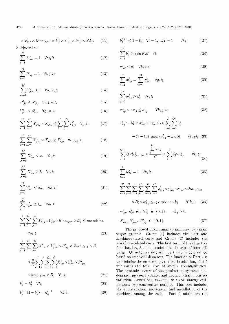
3224 M. Ra�ee and A. Mohamaditalab/Scientia Iranica, Transactions E: Industrial Engineering 27 (2020) 3219{3232
� xtmc � timeijgm �Dti � wtkg � letlk � SAl; (11)
Subjected to:CXc=1
Xtmc = 1 8m; t; (12)
GXg=1
P tijg = 1 8i; j; t; (13)
MXm=1
Y tgm � 1 8g;m; t; (14)
P tijg � �tijg 8i; j; g; t; (15)
Y tgm � �tgm 8g;m; t; (16)
CXc=1
MXm=1
Y tgm �Xtmc �
IXi=1
OiXj=1
P tijg 8g; t; (17)
CXc=1
MXm=1
Y tgm �Xtmc � P tijg 8i; j; g; t; (18)
MXm=1
Xtmc � uc 8c; t; (19)
MXm=1
Xtmc � lc 8c; t; (20)
GXg=1
Y tgm � um 8m; t; (21)
GXg=1
Y tgm � lm 8m; t; (22)
IXi=1
OiXj=1
GXg=1
P tijg�Y tgm�timeijgm�Dti � mcaptime
8m; t; (23)
IXi=1
OiXj=1
GXg=1
Xtmc � Y tgm � P tijg � timeijgm �Dt
i
� qC
CXc=1
IXi=1
OiXj=1
GXg=1
Xtmc�Y tgm�P tijg
�timeijgm �Dti 8c; t; (24)
b1k = h1k 8k; (25)
bt+1k (1� btk) = ht+1
k 8k; t; (26)
ht+1k � 1� btk 8t = 1; :::; T � 1 8k; (27)
KXk=1
btk � minEM 8t; (28)
wtkg � btk 8k; g; t; (29)
KXk=1
wtkg =MXm=1
ytgm 8g; t; (30)
GXg=1
wtkg � btk 8k; t; (31)
wtkg � awg � atkg 8k; g; t; (32)
at+1kg =btk � atkg + wtkg � !1
IXi=1
OiXj=1
�tg
+ (1� btk) max (atkg � !2; 0) 8k; gt; (33)
L�1Xl=1
@l�let(l+1)k �GPg=1
atkg
G�
LXl=1
@l�letlk 8k; t;(34)
LXl=1
letlk = 1 8k; t; (35)
TXt=1
GXg=1
IXi=1
OiXj=1
MXm=1
CXc=1
ptijg�ytgm�xtmc�timeijgm
�Dti�wtkg � opcaptime�btk 8 k; t; (36)
wtkg; htk; b
tk; le
tkl 2 f0; 1g atkg � 0;
Xtmc; Y
tgm; P
tijg 2 f0; 1g: (37)
The proposed model aims to minimize two maintarget groups: Group (1) includes the part andmachine-related costs and Group (2) includes theworkforce-related costs. The �rst term of the objectivefunction, i.e., 3, aims to minimize the trips of inter-cellparts. Of note, an inter-cell part trip is determinedbased on inter-cell distances. The function of Part 4 isto minimize the intra-cell part trips. In addition, Part 5minimizes the total cost of system recon�guration.The dynamic nature of the production systems, i.e.,demand, process routings, and machine characteristicsvariation, causes the machine to move among cellsbetween two consecutive periods. This cost includesthe uninstallation, movement, and installation of themachines among the cells. Part 6 minimizes the

M. Ra�ee and A. Mohamaditalab/Scientia Iranica, Transactions E: Industrial Engineering 27 (2020) 3219{3232 3225
total consumption costs of tools. Moreover, Part 7minimizes the installation/uninstallation costs of toolson di�erent machines. Part 8 minimizes the overallmachine breakdown cost. This cost is determinedaccording to the total processing time of a machineand its breakdown rate. The function of Part 9 isto minimize the workforce hiring/�ring costs. Part10 takes control over the workforce among cells trips.Moreover, workforce salary cost is minimized usingPart 11.
Constraint (12) guarantees that any type of ma-chine is accurately assigned to a given cell. Eq. (13)ensures that the operation of each part can be per-formed by only one tool. It is assumed that a tool canbe installed on only one machine. This constraint isguaranteed by Relation (14). Therefore, the presenceof unused tools in a production period is possible.Relations (15) and (16) ensure that each operationand tool can be assigned to a tool and machine,respectively, with the capability of that installation.Constraints (17) and (18) ensure that the unused toolin a production period cannot be installed on anymachine. The maximum and minimum numbers ofmachines for a cell are represented by Constraints(19) and (20), respectively, which are in the cell sizerange. Moreover, the allocated number of tools toeach machine are presented by Constraints (21) and(22), respectively. The maximum amount of time thateach machine consumes is eliminated by Constraint(23). Moreover, Constraint (24) balances the loadvariations of each cell during a production period. Inthe 1st period, if a worker is hired, he/she shouldbe assigned to working with a machine. This issueis guaranteed by Constraint (25). The workforcehiring/�ring balance between two consecutive periodsis shown in Constraints (26) and (27). Constraint (28),in each manufacturing term, speci�es the least numberof workforce that should be hired. Workforce canwork with a tool only if that workforce is implementedin a production period. Constraint (29) guaranteesthis point. Constraint 30 states that for a tool,workforce should be hired in a production period.Furthermore, if a workforce is hired, he/she shouldbe assigned to some tools (machines) (Constraint(31)). Based on Constraint (32), workforce with aminimum skill value can be selected to work witha machine tool. The workforce learning-forgettinge�ect is assumed according to Constraints (33) and(34). Based on these two constraints, workforce skilllevel must be updated in each production period.Constraint (35) emphasizes that workforce should beranked and given a skill level according to his/herabilities. Workforce time capacity for working ina production period is limited by Constraint (36).Finally, Constraints (37) de�nes the types of modelvariables.
2.4. LinearizationSince the presented MINLP model owing to the exis-tence of nonlinearities in terms 3, 4, 5, 6, 7, 8, 10, and11 and Constraints (17), (18), (23), (24), (26), and (33)is a nonlinear one, here, it was transformed into a linearMIP model using three linearization techniques.
Proposition 1. Consider the pure quadratic 0-1variable Z = X1�X2� :::�Xn, where Xi (i = 1; ::; n)is a binary variable. The amount of variable Z isobviously 1 if and only if all other variables are 1;otherwise 0 [8]. The mentioned mathematical view isformulated below by utilizing some new supplementarylimitations.
Z � Xi 8i = 1; ::; n; Z �nXi=1
Xi � (n� 1):
Proposition 2. Consider the variable Z = X � Yin which X and Y are binary and integer positivevariables, respectively. Utilizing some new auxiliaryconstraints transforms the model into a linear form.The needed limitations are mentioned as follows:Z �M �X; Z � Y ;
Z � Y � (1�X) M ; Z � 0 and int:
Proposition 3. Consider the term:min T;
St :
T = max (X; a);
where X is a variable. By introducing some newauxiliary constraints, the mentioned nonlinear termcould be converted into a linear one. The neededlimitations are mentioned as follows:T � X; T � a:
Accordingly, new variables are de�ned as follows:PXY 1tijgmc=xtmcy
tgmp
tijgx
tm0c0y
tg0m0p
ti(j+1)g0 ; (38)
PXY 2tijgmc=xtmcytgmp
tijgx
tm0cy
tg0m0p
ti(j+1)g0 ; (39)
XXtmcc0 = xtmcx
t+1mc0 ; (40)
Y Xtgmc = ytgmx
tmc; (41)
PY tijgm = ptijgytgm; (42)
PXY tijgmc = ptijgxtmcy
tgm; (43)
Y Y tgmm0 = ytgmyt+1gm0 ; (44)
WW tkgg0 = wtkgw
tkg0 ; (45)
WLtkgl = wtkgletlk; (46)

3226 M. Ra�ee and A. Mohamaditalab/Scientia Iranica, Transactions E: Industrial Engineering 27 (2020) 3219{3232
Btk = bt+1k � (1� btk); (47)
Z = max(atkg � !2; 0); (48)
BAtkg = btk � atkg; (49)
BZtk = (1� btk)� Z: (50)
The following supplementary limitations shouldbe considered along with the previous model:
PXY 1tijgmc � Y Xtgmc + ptijg + Y Xt
g0m0c0
+ pti(j+1)g0 � 3; (51)
PXY 1tijgmc � Y Xtgmc; (52)
PXY 1tijgmc � ptijg; (53)
PXY 1tijgmc � Y Xtg0m0c0 ; (54)
PXY 1tijgmc � pti(j+1)g0 ; (55)
PXY 2tijgmc � Y Xtgmc + ptijg + Y Xt
g0m0c
+ pti(j+1)g0 � 3; (56)
PXY 2tijgmc � Y Xtgmc; (57)
PXY 2tijgmc � ptijg; (58)
PXY 2tijgmc � Y Xtg0m0c; (59)
PXY 2tijgmc � pti(j+1)g0 ; (60)
XXtmcc0 � xtmc + xt+1
mc0 � 1; (61)
XXtmcc0 � xtmc; (62)
XXtmcc0 � xt+1
mc0 ; (63)
Y Xtgmc � ytgm + xtmc � 1; (64)
Y Xtgmc � ytgm; (65)
Y Xtgmc � xtmc; (66)
PY tijgm � ptijg + ytgm � 1; (67)
PY tijgm � ptijg; (68)
PY tijgm � ytgm; (69)
PXY tijgm � xtmc + PY tijgm � 1; (70)
PXY tijgm � PY tijgm; (71)
PXY tijgm � xtmc; (72)
WPXY tijkgm � wtkg + PXY tijgm � 1; (73)
WPXY tijkgm � wtkg; (74)
WPXY tijkgm � PXY tijgm; (75)
Y Y tgmm0 � ytgm + yt+1gm0 � 1; (76)
Y Y tgmm0 � ytgm; (77)
Y Y tgmm0 � yt+1gm0 ; (78)
WW tkgg0 � wtkg + wtkg0 � 1; (79)
WW tkgg0 � wtkg; (80)
WW tkgg0 � wtkg0 ; (81)
WLtkgl � wtkg + letlk � 1; (82)
WLtkgl � wtkg; (83)
WLtkgl � letlk; (84)
WLPXY tijkgml �WLtkgl + PXY tijgm � 1; (85)
WLPXY tijkgml �WLtkgl; (86)
WLPXY tijkgml � PXY tijgm; (87)
WYXtkgg0mm0cc0 �WW t
kgg0 + Y Y tgmm0
+XXtmcc0 � 2; (88)
WYXtkgg0mm0cc0 �WW t
kgg0 ; (89)
WYXtkgg0mm0cc0 � Y Y tgmm0 ; (90)
WYXtkgg0mm0cc0 � XXt
mcc0 ; (91)
Btk � bt+1k + (1� btk)� 1; (92)
Btk � bt+1k ; (93)
Btk � (1� btk); (94)
Z � atkg � !2; (95)
Z � 0; (96)
BAtkg � atkg �M1(1� btk); (97)
BAtkg � atkg; (98)
BAtkg �M1 � btk; (99)
BZtk � Z �M1[1� (1� btk)]; (100)
BZtk � Z; (101)

M. Ra�ee and A. Mohamaditalab/Scientia Iranica, Transactions E: Industrial Engineering 27 (2020) 3219{3232 3227
BZtk �M1 � (1� btk): (102)
Therefore, the linear version of the MIP model can alsobe considered.
min Model 2 =TXt=1
IXi=1
OiXj=1
GXg;g0=1
MXm;m0=1
Xc;c6=c0
PXY 1tijgmc �Dti � disc;c0 �MCi; (103)
+TXt=1
IXi=1
OiXj=1
GXg;g0=1
CXc=1
Xm;m 6=m0
PXY 2tijgmc�Dti ; (104)
+T�1Xt=1
MXm=1
Xc;c6=c0
XXtmcc0 � disc;c0 � SM; (105)
+TXt=1
MXm=1
IXi=1
OiXj=1
GXg=1
PY tijgm �Dti � ijg; (106)
+T�1Xt=1
GXg=1
Xm;m 6=m0
Y Y tgmm0 � SG; (107)
+TXt=1
MXm=1
IPi=1
OiPj=1
GPg=1PY tijgm� timeijgm�Dt
i
MTBFm�Bm; (108)
KXk=1
�h1k �H�+ TX
t=2
KXk=1
�htk�H + (1�btk)� F �; (109)
TXt=1
KXk=1
Xg;g0
Xm;m0
Xc;c0 6=c
WYXtkgg0mm0cc0�disc;c0 ; (110)
+MXm=1
TXt=1
KXk=1
LXl=1
GXg=1
WLPXY tijkgml � timeijgm
�Dti � SAl: (111)
The above model is conditional on the unaltered set ofConstraints (12){(17), (19){(22), (25), (27){32), (34),(35) and the new auxiliary Constraints (51){(92).
Moreover, the set of Constraints (17), (18), (23),(24), (26), and (33) is replaced by:
CXc=1
MXm=1
Y Xtgmc �
IXi=1
OiXj=1
P tijg 8g; t; (112)
CXc=1
MXm=1
Y Xtgmc � P tijg 8i; j; g; t; (113)
IXi=1
OiXj=1
GXg=1
PY tijgm � timeijgm �Dti � captime
8m; t; (114)
Btk = ht+1k 8k; t; (115)
at+1kg = !1
IXi=1
OiXj=1
WPXY tijkgm +BZtk +BAtkg
8k; g; t; (116)
and the last set of constraint, i.e., Constraint (36) isreplaced by:
wtkg; htk; b
tk; le
tkl; B
tk; p
tijg;WW t
kgg0 ;WLtkgl; xtmc; y
tgm;
PY tijgm; PXYtijgmc; PXY 1tijgmc; PXY 2tijgmc;
WPXY tijkgm;WLPXY tijkgml;WY Xtkgg0mm0cc0 ;
XXtmcc0 ; Y X
tgmc; Y Y
tgmm0 2 f0; 1gBAtkg;
BZtk; z; atkg � 0: (117)
3. Computational experience
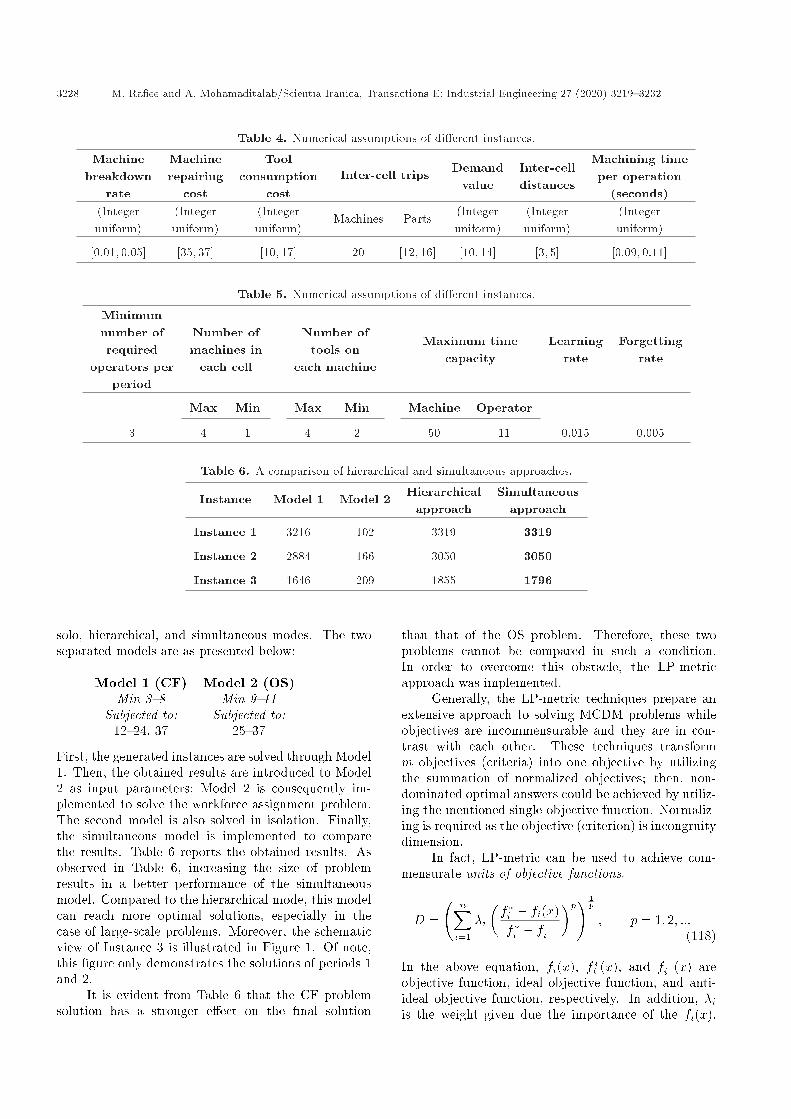
In the following, the experiments conducted to evaluatethe capability of solving the CMS problem through thepresented model and applied approach are presented.Three instances were randomly generated. Experi-ments were performed on the implemented and solvedmodel on a Core i5 PC with 1 GB of RAM using GAMS23.5. The input data of generated instances are givenin Tables 3{5. According to Bagheri and Bashiri [8],to obtain an optimal solution, two problems of CF andworkforce assignment should be simultaneously solved.To this end, the present paper aims to separate andsolve these two problems in three modes, namely the
Table 3. Numerical assumptions of di�erent instances
InstanceNumber ofmachines
Number ofparts
Number oftime periods
Number ofcells
Number ofoperators
Number ofmachine tools
Instance 1 3 2 3 2 4 5Instance 2 4 4 3 2 6 7Instance 3 3 4 3 2 8 10
3228 M. Ra�ee and A. Mohamaditalab/Scientia Iranica, Transactions E: Industrial Engineering 27 (2020) 3219{3232
Table 4. Numerical assumptions of di�erent instances.
Machinebreakdown
rate
Machinerepairing
cost
Toolconsumption
costInter-cell trips Demand
valueInter-celldistances
Machining timeper operation
(seconds)(Integeruniform)
(Integeruniform)
(Integeruniform)
Machines Parts (Integeruniform)
(Integeruniform)
(Integeruniform)
[0:01; 0:05] [35; 37] [10; 17] 20 [12; 16] [10; 14] [3; 5] [0:09; 0:11]
Table 5. Numerical assumptions of di�erent instances.
Minimumnumber ofrequired
operators perperiod
Number ofmachines in
each cell
Number oftools on
each machine
Maximum timecapacity
Learningrate
Forgettingrate
Max Min Max Min Machine Operator
3 4 1 4 2 50 11 0.015 0.005
Table 6. A comparison of hierarchical and simultaneous approaches.
Instance Model 1 Model 2 Hierarchicalapproach
Simultaneousapproach
Instance 1 3216 102 3319 3319
Instance 2 2884 166 3050 3050
Instance 3 1646 209 1855 1796
solo, hierarchical, and simultaneous modes. The twoseparated models are as presented below:
Model 1 (CF) Model 2 (OS)Min 3{8 Min 9{11
Subjected to: Subjected to:12{24, 37 25{37
First, the generated instances are solved through Model1. Then, the obtained results are introduced to Model2 as input parameters; Model 2 is consequently im-plemented to solve the workforce assignment problem.The second model is also solved in isolation. Finally,the simultaneous model is implemented to comparethe results. Table 6 reports the obtained results. Asobserved in Table 6, increasing the size of problemresults in a better performance of the simultaneousmodel. Compared to the hierarchical mode, this modelcan reach more optimal solutions, especially in thecase of large-scale problems. Moreover, the schematicview of Instance 3 is illustrated in Figure 1. Of note,this �gure only demonstrates the solutions of periods 1and 2.
It is evident from Table 6 that the CF problemsolution has a stronger e�ect on the �nal solution
than that of the OS problem. Therefore, these twoproblems cannot be compared in such a condition.In order to overcome this obstacle, the LP-metricapproach was implemented.
Generally, the LP-metric techniques prepare anextensive approach to solving MCDM problems whileobjectives are incommensurable and they are in con-trast with each other. These techniques transformm objectives (criteria) into one objective by utilizingthe summation of normalized objectives; then, non-dominated optimal answers could be achieved by utiliz-ing the mentioned single-objective function. Normaliz-ing is required as the objective (criterion) is incongruitydimension.
In fact, LP-metric can be used to achieve com-mensurate units of objective functions.
D =
nXi=1
�i�f�i � fi(x)f�i � f�i
�p! 1p
; p = 1; 2; :::(118)
In the above equation, fi(x), f�i (x), and f�i (x) areobjective function, ideal objective function, and anti-ideal objective function, respectively. In addition, �iis the weight given due the importance of the fi(x).

M. Ra�ee and A. Mohamaditalab/Scientia Iranica, Transactions E: Industrial Engineering 27 (2020) 3219{3232 3229
Figure 1. The schematic view of the solution to Instance 3.
Table 7. The trade-o� matrix of Cell Formation (CF) and OS problems.
Positive ideal solutions Negative ideal solutions
f1 f2 f1 f2
f1 f�1 = 1569:979 273 f�1 = 17968:82 271f2 13156.49 f�2 = 209:484 10634.63 f�2 = 549:491
Attempts were made to minimize the distance betweenthe ideal and anti-ideal pursuant to the constraints anddiscover the non-dominated solution. Therefore, in Eq.(118), LP-metric represents the distance between F (x)and F �(x).
Based on this approach, the trade-o� matrix canbe generated, as shown in Table 7.
By changing the �i value, which represents theweight considered for each of the aforementioned prob-lems, the Pareto optimal solution can be obtained, asshown in Figure 2.
As observed in this �gure, workforce-related costshave a signi�cant impact on the CF solution. In orderto analyze the OS problem in detail, expert workforcewho worked only with a machine tool without anytraining cost was carefully supervised. The salary ofthis workforce was naturally higher than that of others.In this situation and based on the results, workforce
Figure 2. The pareto solution to Cell Formation (CF)and OS problems.
with a lower skill level was selected to be trained howto work with that machine tool. With a decrease in thesalary of the expert workforce, he/she was selected asa machine tool workforce.

3230 M. Ra�ee and A. Mohamaditalab/Scientia Iranica, Transactions E: Industrial Engineering 27 (2020) 3219{3232
Figure 3. Cost sensitivity analysis versus demand rate.
Figure 4. The increasing rate of demand vs. the numberof operations assigned to a machine (period 1) Instance).
In addition, it can be concluded that any changein the demand value might signi�cantly a�ect theessential cost terms, shown in Figure 3. Accordingto this Figure, with an increase in the demand value,the inter-cell part trip cost has exponentially increased.Hence, a decision-maker should control the demandvalue to avoid extra inter-cell part trip costs. Moreover,a meticulous maintenance plan can decrease the rate ofmachine breakdown in high-demand companies.
Machines are the second main manufacturingresources required to be analyzed in detail. Machinebreakdown and demand rate are of considerable signif-icance in machine implementation in a manufacturingcompany. Figure 4 illustrates the increasing rate of
demand on the total number of operations assigned toa machine in a production period (Instance 1).
According to this Figure 4, Machine 3 can processa maximum number of 4 operations in a productionperiod. As mentioned earlier, a machine cannot beinterrupted while processing a task. According to theinput data, the rate of breakdown in machine 3 ishigher than that in the other two machines. Therefore,it is preferable that this machine would process only 3operations, even in a high-demand situation.
To adjust real-world cellular production systemmodels, it is required to add more variables andlimitations to the model, which will demand a lotof time to solve such models by time, memory, andprocessing power. As a result, nowadays, modernmethods are applied to a Genetic Algorithm (GA). AGA is part of random search techniques that are usedto solve NP-complete problems, such as cell-systemproduction models.
In this section, MATLAB software (GA tool-Genetic algorithm GUI) was utilized to solve the com-plexities of the hierarchical and simultaneous modelwith the GA to evaluate the performance of the modelsin vaster dimensions. In Table 8, the dimensions of 4numerical instances are solved using GA. The obtainedresults are given in both Table 9 and Figure 5. Ofnote, the simulation model has achieved a better resultthan the hierarchical model. By developing a varietyof the dimensions of the models, the deviation of theoptimum values obtained in the two models becomesmore signi�cant than ever.
Due to the lack of a similar article and a real casestudy in Iran, the sensitivity analysis of one of theexamined examples mentioned in the paper was per-formed to validate the model. For instance, in Instance4, by assuming that the dimensions of the model were
Table 8. Numerical assumptions of instance.
Instance Number ofmachines
Number ofparts
Number oftime periods
Number ofcells
Number ofoperators
Number ofmachine tools
Instance GA 1 10 20 3 2 13 2
Instance GA 2 15 25 3 3 14 3
Instance GA 3 20 27 3 3 15 5
Instance GA 4 25 30 3 5 16 6
Table 9. A comparison of hierarchical and simultaneous approaches (genetic algorithm).
Instance Model 1 Model 2 Hierarchicalapproach
Simultaneousapproach
Instance GA 1 7560 1003 8563 8294Instance GA 2 8640 2845 11485 9869Instance GA 3 10380 5004 15384 10384Instance GA 4 15230 9384 24614 17974

M. Ra�ee and A. Mohamaditalab/Scientia Iranica, Transactions E: Industrial Engineering 27 (2020) 3219{3232 3231
Figure 5. Functional behavior in the genetic algorithm.
Figure 6. Cost sensitivity analysis versus demand rate inthe genetic algorithm.
constant, the sensitivity of the model parameters wasanalyzed. For example, the sensitivity analysis of thedemand parameter that changed all decision variablesand optimal values is shown in Figure 6. Some quanti-ties were not signi�cantly di�erent in costs such as thecost of installing machines and cellular con�gurations.In other cases, the breakdown of machines and cost ofintercellular mobility were considerably high; therefore,the resulting changes seem reasonable.
4. Conclusion
The present paper proposed a new-fangled model to de-sign an e�cient Cellular Manufacturing System (CMS).The basic assumptions of the proposed model were theincorporation of machine tools, machine breakdown,and the workforce learning-forgetting e�ect. To thebest of the authors' knowledge, only a few researchershave focused on such real-world parameters. In termsof both computational time and optimality, the exper-imental results veri�ed the e�ciency of the proposedapproach. Moreover, analytical experiments wereperformed to assess the sensitivity of the presentedmodel and it could be concluded that the machinefailure played a key role in elevating the performanceof CMS, especially in companies of high demands.In addition, workforce-related costs were found tohave a strong impact on the cell formation solution.Another sensitivity analysis of the proposed model
revealed the impact of changing demand on the rateof machine utilization. In other words, by increasingthe demand value, the machine with the minimumbreakdown cost value was implemented more oftenthan other ones. Besides, nowadays, in the competitiveatmosphere of the world, the workforce representsthe main production resources. Hence, analyzingand proposing new models is essential to optimallysolve OS problems. In this paper, some workforce-related issues including hiring, �ring, their salary,training, and the workforces' learning-forgetting e�ectwere taken into account. Given all these considerations,the developed mathematical model could be employedfor factories with the capability of having a cellulardesign. In fact, numerous industrial factories suchas car manufacturers with a rich diversity in theirproduct types and uctuations in the demand value canemploy the proposed model with the aim of designingan optimal CMS via the minimum amount of costs.The main objective of this research was to considersome real-world production elements to be applied tomany factories.
As a guideline for future studies, it would bemotivating to develop some solution approaches tooptimally solve the model. Moreover, incorporatingother real-world industrial factors such as intra-cell GLand machine duplication in providing a framework canbe of great value for future research. Additionally,the concept of uncertainty can be considered in theprovided framework. As an instance, uncertainty inthe demand value or the processing time is one of themain issues in real world application and thus, it canbe explored in more detail in future studies.
Acknowledgement
The authors would like to state their gratitude to IranNational Science Foundation (INSF) for all their kindsupport of the present project.
References
1. Liu, C., Wang, J., and Leung, J.Y.T. \Integratedbacteria foraging algorithm for cellular manufacturingin supply chain considering facility transfer and pro-duction planning", Applied Soft Computing, 62, pp.602{618 (2018).
2. Askin, R.G. \Contributions to the design and analy-sis of cellular manufacturing systems", InternationalJournal of Production Research, 51, pp. 6778{6787(2013).
3. Ameli, M.S.J. and Arkat, J. \Cell formation withalternative process routings and machine reliabilityconsideration", The International Journal of AdvancedManufacturing Technology, 35, pp. 761{768 (2008).
4. Bulgak, A.A. and Bektas T. \Integrated cellular manu-facturing systems design with production planning and

3232 M. Ra�ee and A. Mohamaditalab/Scientia Iranica, Transactions E: Industrial Engineering 27 (2020) 3219{3232
dynamic system recon�guration", European Journal ofOperational Research, 192, pp. 414{428 (2009).
5. Mehdizadeh, E., Niaki S.V.D., and Rahimi, V. \Avibration damping optimization algorithm for solvinga new multi-objective dynamic cell formation problemwith workers training", Computers & Industrial Engi-neering, 101, pp. 35{52 (2016).
6. Mahdavi, I., Aalaei, A., Paydar, M.M., and Soliman-pur, M. \Designing a mathematical model for dynamiccellular manufacturing systems considering productionplanning and worker assignment", Computers & Math-ematics with Applications, 60, pp. 1014{1025 (2010).
7. Aryanezhad, M.B., Deljoo, V., and Mirzapour Al-e-Hashem, S. \Dynamic cell formation and the workerassignment problem: a new model", The InternationalJournal of Advanced Manufacturing Technology, 41,pp. 329{342 (2009).
8. Bagheri, M. and Bashiri M. \A new mathematicalmodel towards the integration of cell formation withworkforce assignment and inter-cell layout problemsin a dynamic environment", Applied MathematicalModelling, 38, pp. 1237{1254 (2014).
9. Javadi, B., Jolai, F., Slomp, J., Rabbani, M., andTavakkoli- Moghaddam, R. \An integrated approachfor the cell formation and layout design in cellularmanufacturing systems", International Journal of Pro-duction Research, 51, pp. 6017{6044 (2013).
10. Bagheri, M., Sadeghi, S., and Saidi-Mehrabad, M. \Abenders' decomposition approach for dynamic cellularmanufacturing system in the presence of unreliablemachines", Journal of Optimization in Industrial En-gineering, 17, pp. 37{49 (2015).
11. Bayram, H. and S�ahin, R. \A comprehensive math-ematical model for dynamic cellular manufacturingsystem design and linear programming embedded hy-brid solution techniques", Computers & IndustrialEngineering, 91, pp. 10{29 (2016).
12. Azadeh, A., Ravanbakhsh, M., Rezaei-Malek, M.,Sheikhalishahi, M., and Taheri-Moghaddam, A.\Unique NSGA-II and MOPSO algorithms for im-proved dynamic cellular manufacturing systems con-sidering human factors", Applied Mathematical Mod-elling, 48, pp. 655{672 (2017).
13. Liu, C., Wang, J., and Leung, J.Y.T. \Worker as-signment and production planning with learning and
forgetting in manufacturing cells by hybrid bacteriaforaging algorithm", Computers & Industrial Engi-neering, 96, pp. 162{179 (2016).
14. Mehdizadeh, E. and Rahimi, V. \An integrated mathe-matical model for solving dynamic cell formation prob-lem considering workforce assignment and inter/intracell layouts", Applied Soft Computing, 42, pp. 325{341(2016).
15. Ra�ei, H. and Ghodsi, R. \A bi-objective mathemat-ical model toward dynamic cell formation consideringlabor utilization", Applied Mathematical Modelling,37, pp. 2308{2316 (2013).
16. Sakhaii, M., Tavakkoli-Moghaddam, R., Bagheri, M.,and Vatani, B. \A robust optimization approach for anintegrated dynamic cellular manufacturing system andproduction planning with unreliable machines", Ap-plied Mathematical Modelling, 40, pp. 169{191 (2016).
17. Nouri, H. \Development of a comprehensive model andBFO algorithm for a dynamic cellular manufacturingsystem", Applied Mathematical Modelling, 40, pp.1514{1531 (2016).
Biographies
Majid Ra�ee received his BSc degree in IndustrialEngineering from Isfahan University, Isfahan, Iran in2003 and his MSc and PhD degrees in Industrial Engi-neering from Sharif University of Technology, Tehran,Iran in 2006 and 2013, respectively. In 2013, hejoined the Department of Industrial Engineering atSharif University of Technology, Tehran, Iran as anAssistant Professor. Dr. Ra�ee's research interestsinclude stochastic programming, operations research,mathematical programming, quality management, andquality control.
Atye Mohammaditalab received his BSc degreein Industrial Engineering from Sharif university ofTechnology, Tehran, Iran, and his MSc degree in Math-ematics from University of Tehran, Tehran, Iran in2013 and 2016, respectively. Her main areas of interestare integer programming, mathematical modeling, andoptimization.