Investigation and validation of wake model combinations for large windfarm modelling in neutral boundary layers

Eric TROMEUR(1), Sophie PUYGRENIER(1),Stéphane SANQUER(1)

(1) Meteodyn France, 14bd Winston Churchill, 44100, Nantes, France

ABSTRACT

An original approach consisting on the combination of two wake patterns – a single wake model with a neutralboundary layer modification - is investigated in order to model large wind farm wake effect. Sensitivity studiesof boundary layer parameters are carried out to optimize the velocity and power corrections whatever the type ofwind farms and the wind directions. Two single wake models (Park and Fast EVM) were combined to a refinedboundary layer model and validated against measurements and four standard wake models. This very promisingmodel combination allows us to take into account the slowdown in large wind farms.

1 Introduction

When air under neutral conditions flows from one surface through a wind turbine with adifferent roughness, the air is slowed [1][2], an internal boundary layer growing downwindfrom the roughness change [3][4][5]. The region in the flow behind the turbine is called thewake of a wind turbine. Its effects are seen as wake effects.

It is thus important to evaluate and model these effects and boundary layer changes toestimate the amount of power remaining downstream of the turbine.

Wind resource softwares like WindFarmer [6], Wakefarm [7], WaSP [8][9], NTUA [10] orMeteodyn WT [11] were evaluated for small wind farms [12] or single wakes [13]. However,it has become apparent that standard single wake models as Park [14][15] and Fast EVM [16]models tend to underestimate wake losses in large wind farms as offshore arrays [17].

In this paper, an original approach consisting on the combination of two wake patterns – asingle wake model with a neutral boundary layer modification - is investigated and validatedagainst measurements and four standard wake models as in [18] in order to model large windfarm wake effect and compute velocity deficit.

2 Measurements

Wind turbine power production data from two large offshore wind farms, Horns Rev andNysted, are used to validate our large wind farm model results as in [18]. The normalizedpower (with respect to the power of the first wind farm column, see figure 1) at each turbineis calculated for seven wind direction sectors centered on an exact wind farm row (ER) ( 270°+/- 2.5° at Horns Rev and 278° +/- 2.5° at Nysted), and for mean wind directions of +5°,+10°, and +15° and -5°, -10°, and -15° from ER. Flow down at ER thus represents the likelymaximum wake effect, while the wind directions that are slightly offset from ER assist inassessing the wake width.

In both cases, wake effects is evaluated for a free-stream velocity mainly coming from thewest (not shown) and equal to 8 m.s-1 as in [18].

Figure 1: Horns rev wind farm layout [18].

3 Large wind farm model: parametrization and activation

Single wake models don’t consider the change of the atmospheric boundary layer by theadditional roughness associated with wind turbines. An original approach consists oncalculating the velocity deficit in each point of the wind farm by combining a wake effectfrom a single wind turbine with the boundary layer modification.

Two single wake models (Park and Fast EVM) used in Meteodyn WT software [11] and alarge wind farm model taking into account inner boundary layer (IBL) modification arecombined and named WT Park+IBL and WT Fast EVM+IBL.

The boundary layer profile is then expressed as a function of the equivalent roughness z'0 andthe wind position relative to the upstream turbine.

Three steps and sensitivity studies are necessary to optimize and compute the velocity deficitvia combined wake models:

1. Equivalent roughness z'0 computation

2. Boundary layer profile estimation

3. Large wind farm model activation

3.1 Roughness z'0 influence

The equivalent roughness z'0 is calculated with the method of Frandsen [19][20] for eachwind direction and wind speed at each turbine. It depends on the spacing between two rowsof wind turbines along the wind direction Sd and the crosswind direction Sc. Sc has a hugeinfluence on the roughness (example on Figure 2 for the wind turbine WT74 at the HornsRev with Sd = 7). It impacts directly the normalized power with respect to the wind turbineWT04, going down to 10% if Sc = 3 (see Table 1).

An algorithm has been developed to optimize Sc and Sd whatever the type of wind farms andthe wind directions. Figure 3 presents an example of Sc and Sd evolutions at Horns Rev forER incidence (other incidences not shown here).

Figure 2: Frandsen roughness function of wind speed and Sc with Sd=7 at ER incidence and wind turbine WT74at Horns Rev

Table 1: Normalized power evolution function of z'0, Sc and Sd

The number of upstream wind turbines for a specific position is increasing for a wind turbinegoing far away from the first column of the array. Sc and Sd are homogeneous over the allwind farm considering at least one wind turbine is detected upstream. Sc and Sd has beenfound equal to 7 for both wind farms in Denmark.

3.2 Inner boundary layer influence

The velocity deficit coefficient correction is the ratio between the wind speed in the IBL andthe wind speed taken at the same height before the roughness change. However, an offsetHstart (function of the fetch and z’0.) from which the boundary layer starts and the IBL heighthibl influence it. Sensitivity studies of Hstart and hibl are then carried out at Horns Rev with thetwo combined wake models in order to optimize wind speed and power corrections:

As shown in Table 2, the more Hstart is low, the more velocity and power deficits arelow. On the contray to [6] proposing Hstart = 2/3 hhub (with hhub the hub height), theoptimum Hstart is equal to zero, meaning the inner boundary layer influence starts fromthe ground.

According to [21], 0.05h ≤ hibl ≤ 0.09h, where h is the boundary layer height.Comparisons between both combined models and observations in Figure 4 show abetter agreement for hibl=0.05h (case B/) against 9% of h in [6]. The same is observedfor all other directions, except for ER-15° and ER-10° (not shown).

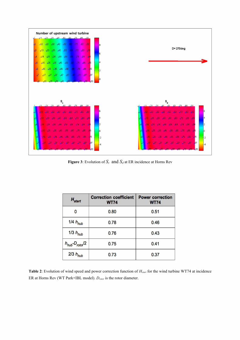
Figure 3: Evolution of Sc and Sd at ER incidence at Horns Rev

Table 2: Evolution of wind speed and power correction function of Hstart for the wind turbine WT74 at incidence

ER at Horns Rev (WT Park+IBL model). Drotor is the rotor diameter.

Figure 4: Normalized power at ER +15° at Horns Rev for ibl = 0.09 (A/) and 0.05 (B/).

All these optimized parameters are considered by default in the next validation section 4.

3.3 Large wind farm model activation

A geometric measure of turbine density is used to activate the large wind farm model.Considering the turbine density for 5° sectors, the large wind farm correction to ambient windspeed is applied if there is at least one turbine in the selected sector. Moreover, this model isalways activated from the fourth wind farm column.

Finally, the velocity deficit is computed as the velocity deficit minimum taken between thelarge wind farm model and the single wake Park or Fast EV models.

Figure 5: Mean normalized power from Horns Rev (top), Nysted (down) and model simulations for the second (left) and the eighth (right) columns of wind turbines.

4 Model comparisons with offshore wind farm data

A model intercomparison is performed at the two offshore wind farms for four different wakemodels as in [18] and the two combined models.

4.1 Wake width

As for other models, WT Park and Fast EVM models+IBL capture well the wake width at thesecond column of wind turbines (Figure 5) and show greater agreement with the observedwake depth than WaSP though both overestimate (respectively underestimate) the magnitudeof the wake width at Horns Rev (Nysted).

For the entire wind farm (column 8), normalized powers of both combined models fit betterwith observations than other models even if they tend to overestimate (underestimate) thepower for sectors less (greater) than ER.

In general, the root-mean-square error (RMSE) of normalized power shown in Table 3indicates that WT Park+IBL and WT Fast EVM+IBL models perform better (i.e., exibit lowerRMSE) for direct flow down the row (i.e, ER) than for oblique angles.

4.2 Power deficit by downwind distance

In Figures 6 and 7, both combined models appear to capture the shape of power deficit as afunction of distance into both wind farms. In general, WT Fast EMV+IBL model has a verygood agreement with Windfarm and WindFarmer models, being even better at an incidentwind directions of 255°, 260°, 275°, 285° for Horns Rev and 263°, 268°, 273°, 283° forNysted.

Table 3: RMSE of normalized power from the models vs observations at Horns Rev (top) and Nysted (down).

5 Conclusion

Investigation for large wind farm modelling under neutral conditions have been carried out bycombination of two single wake models (Park and Fast EVM) with a refined version ofboundary layer models based on [6] and [21].

Sensitivity studies of IBL parameters (Sc , Sd, Hstart and hibl) allow us to design optimumcombination whatever the type of wind farms and wind directions.

The large wind farm models are then validated against measurements and four standard wakemodels, suggesting combined wake models well represent the losses in those wind farms.

In the future, a linear combination of single wake models with the boundary layermodification will be investigated to compute velocity and power deficits.

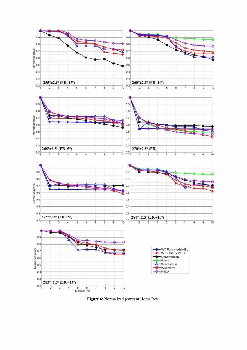
Figure 6: Normalized power at Horns Rev.

Figure 7: Normalized power at Nysted.

References

[1] Crespo, A, J. Hernandez and S. Frandsen, Survey of modelling methods for wind turbinewakes and wind farms, Wind Energy, Vol. 2, pp. 1-24, 1999.

[2] Vermeer, L.J., J.N. Sørensen and A. Crespo, Wind turbine wake aerodynamics, Progressin Aerospace Sciences, Vol. 39, pp. 467-510, 2003.

[3] Bradley, E.F., A micrometeorological study of velocity profiles and surface drag in theregion modified by a change in surface roughness, Quart. J. R. Met. Soc., 94, pp. 361-379,1968.

[4] Jensen, N.O., Change of surface roughness and the planetary boundary layer, Qart. J. R.Met. Soc., 104, pp. 351-356, 1978.

[5] Rao, K.S., J.C. Wyngaard and D.R. Coté, The structure of the two-dimensional internalboundary layer over a sudden change of surface roughness, J. Atmos. Sci., 26, pp. 432-440,1974.

[6] Schlez W., and A. Neubert, New developments in large wind farm modelling, Proc.European Wind Energy Conf., Marseille, France, EWEA PO.167, 8 p., 2009.

[7] Schepers, J.G., ENDOW: Validation and improvement of ECN’s wake model, EnergyResearch Center for the Netherlands rep. ECN-C-03-034, 113 p., 2003.

[8] Mortensen, N.G., Heathfield, D.N., Myllerup, L., L. Landberg and O. Rathmann, Windatlas analysis and application program: WAsP 8 help facility, Risø National Laboratory,Roskilde, Denmark, 2005.

[9] Rathmann, O., R.J.Barthelmie and S.T. Frandsen, Turbine wake model for wind resourcesoftware, Proc. European Wind Energy Conf., Athens, Greece, EWEA, BL3.313, 2006.

[10] Magnusson, M., K.G. Rados and S.G. Voutsinas, A study of the flow down stream of awind turbine using measurements and simulations, Wind Eng., 20, 389-403, 1996.

[11] Li, R., D. Delaunay, and Z. Jiang, A new Turbulence Model for the Stable BoundaryLayer with Application to CFD in Wind Resource Assessment, EWEA Proceedings, 9 p.,Paris, France, 17-20 November, 2015.

[12] Barthelmie, R.J. And Coauthors, Efficient development of offshore windfarms(ENDOW): Modelling wake and boundary layer interactions, Wind Energy, 7, 225-245, 2004.

[13] Barthelmie, R.J., Folkerts, L., Rados, K., Larsen, G.C., Pryor, S.C., Frandsen, S., B.Lange, and G. Schepers, Comparison of wake model simulations with offshore wind turbinewake profiles measured by sodar, J. Atmos. Oceanic Technol., 23, 88-901, 2006.

[14] Jensen, N.O., A note on wind generator interaction, Technical report from the RisøNational Laboratory (Risø-M-2411), Roskilde, Denmark, 16 p., 1983.

[15] Katic, I., J, Hojstrup, N.O. Jensen, A simple model for cluster efficiency, EWECProceedings, Rome, Itally, 5 p., 1986.

[16] Ainslie, J.F., Calculating the flowfield in the wake of wind turbines, I. Wind Eng. AndInd Aero., Vol. 27, pp. 213-224, 1988.

[17] Beaucage, P., Robinson, N., M. Brower and C. Alonge, Overview of six commercial andresearch wake models for large offshore wind farms, EWEA Proceedings, 10 p., Copenhagen,Germany, 16-19 April, 2012.

[18] Barthelmie, R.J., Pryor; S.C., Frandsen, S.T., Hansen, K.S., Schepers, J.G., Rados, K.,Schlez, W., Neubert, A., L.E. Jensen and S. Neckelmann, Quantifying the Impact of WindTurbines Wakes on Power Output at Offshore Wind Farms, Journal of Atmospheric andOceanic Technology, Vol. 27, pp. 1302-1317, 2010.

[19] Frandsen, S., Barthelmie, R., Pryor, S., Rathmann, O., Larsen, S., Højstrup, J., and M.Thøgersen, Analytical modelling of wind speed deficit in large offshore wind farms. WindEnergy, 9, 2006.

[20] Frandsen, S.T., Turbulence and Turbulence-Generated Structural Loading in WindTurbine Clusters, Technical report from the Risø National Laboratory (Risø-R-1188),Roskilde, Denmark, 130p., 2007.

[21] Larsen, Søren Ejling; Mortensen, Niels Gylling; Sempreviva A. M.; Troen, Ib.; Responseof neutral boundary layers to changes of roughness, Meteorology and Wind EnergyDepartment. Annual Progress Report. 1 January - 31 December 1987 (pp. 15-43). RisøNational Laboratory, Denmark. Forskningscenter Risoe. Risoe-R; No.560), 1988.