ARTICLE IN PRESS

1352-2310/$ - se

doi:10.1016/j.at

�Correspondfax: +612 6125

E-mail addr1Senior Lectu2Reader.

Atmospheric Environment 40 (2006) 984–991

www.elsevier.com/locate/atmosenv

Investigating the mixture of air pollutants associated withadverse health outcomes

Steven Roberts�,1, Michael A. Martin2

Faculty of Economics and Commerce, School of Finance and Applied Statistics, Australian National University,

Canberra ACT 0200, Australia

Received 17 May 2005; accepted 12 October 2005

Abstract

Most investigations of the adverse health effects of multiple air pollutants analyse the time series involved by

simultaneously entering the multiple pollutants into a Poisson log–linear model. Concerns have been raised about this type

of analysis, and it has been stated that new methodologies or models need to be developed for investigating the adverse

health effects of multiple air pollutants. To this end, it has recently been stated that it may be more reasonable to assume

that there is a mixture of pollutants considered harmful to health and that assessing the adverse health effects of an air

pollution mix may be both more meaningful and more tenable than attempting to isolate the effects of individual

pollutants. In this paper, a new model is introduced that is able to reveal the mixture of pollutants associated with an

adverse health outcome and the effect of this mixture on the adverse health outcome. The model is shown to have a

number of advantages over the traditional method of estimating the adverse health effects of multiple air pollutants. In

addition, the model is also shown to be an improvement over a previously proposed, and somewhat ad-hoc, method for

estimating the mixture of pollutants associated with an adverse health outcome.

r 2005 Elsevier Ltd. All rights reserved.

Keywords: Air pollution; Mortality; Time series; Multiple pollutants

1. Introduction

Numerous time series studies have investigatedthe association between daily adverse health out-comes and daily ambient air pollution concentra-tions (Chock et al., 2000; Cifuentes et al., 2000;Goldberg et al., 2003; Kelsall et al., 1997, 2000;

e front matter r 2005 Elsevier Ltd. All rights reserved

mosenv.2005.10.022

ing author. Tel.: +61 2 6125 3470;

0087.

ess: steven.roberts@anu.edu.au (S. Roberts).

rer.

Kwon et al., 2001; Moolgavkar, 2000; Ostro et al.,1999; Roemer and van Wijnen, 2001; Smith et al.,2000a, b; Stieb et al., 2002; Styer et al., 1995). Thesestudies typically fit a Poisson log–linear model toconcurrent time series of daily mortality or morbid-ity, ambient air pollution and meteorologicalcovariates. The fitted models are then used toquantify the adverse health effects of ambient airpollution. Because the US Environmental Protec-tion Agency regulates pollutants independently,most of the current time series research on theadverse health effects of air pollution has focused onestimating the effects of an individual pollutant

.

ARTICLE IN PRESSS. Roberts, M.A. Martin / Atmospheric Environment 40 (2006) 984–991 985

(Dominici and Burnett, 2003). However, due to thepotentially high correlation between ambient airpollutants, the results from studies that focus on asingle pollutant can be difficult to interpret inpractice (Vedal et al., 2003). For example, anobserved positive association could occur becausethe single air pollutant is a proxy for another airpollutant or for a mixture of air pollutants.

To overcome the limitations of single-pollutanttime series studies, a number of studies haveinvestigated the concurrent adverse health effectsof multiple air pollutants (Moolgavkar, 2000; Wonget al., 2002). In the majority of studies of thisnature, the multiple air pollutants are simulta-neously entered into a single Poisson log–linearmodel. The results from these studies are used toisolate the adverse health effects of the individualpollutants. However, one important question thatthese multiple pollutant studies do not answer iswhether there is a mixture of pollutants that isassociated with the adverse health outcome. More-over, it has recently been stated that it may be morereasonable to assume that there is a mixture ofpollutants that is considered harmful to health(Dominici and Burnett, 2003; Moolgavkar, 2003;Stieb et al., 2002). Assessing the adverse healtheffects of an air pollution mix may, therefore, beboth more interpretable and more feasible thanattempting to isolate the effects of individualpollutants. The development of new methodologyor models to concurrently estimate the adversehealth effects of multiple air pollutants has beenidentified by statisticians, epidemiologists and pol-icymakers as an important area of future research(Cox, 2000; Dominici and Burnett, 2003).

In this paper, a new model is introduced thatreveals the mixture of pollutants associated with anadverse health outcome and the effect of this mixtureon that outcome. This new model uses time seriesdata to assign each air pollutant a weight whichindicates the pollutant’s contribution to the airpollution mixture that is associated with the adversehealth outcome under investigation. The model isillustrated by applying it to time series data from nineUnited States counties for the period 1987–2000.

2. Materials and methods

2.1. Materials

The data used in this paper were obtained fromthe publicly available National Morbidity, Mortal-

ity, and Air Pollution Study (NMMAPS) database.The data extracted consists of concurrent daily timeseries of mortality, weather and air pollution fornine cities in the United States for the period1987–2000. The nine cities selected had a relativelylarge number of days with measurements for all fiveair pollutants considered. Many of the cities in theNMMAPS database do not collect data on all fiveair pollutants and/or have a large number of dayswith missing air pollutant concentrations.

The mortality time series data, aggregated at thelevel of county, are non-accidental daily deaths ofindividuals aged 65 and over. Deaths of non-residents were excluded from the mortality counts.The weather time series data are 24 h averages oftemperature and dew point temperature, computedfrom hourly observations.

The five air pollutants considered are particulatematter of less than 10 mm in diameter (PM), ozone(O3), sulphur dioxide (SO2), carbon monoxide (CO)and nitrogen dioxide (NO2). For PM, SO2, CO andNO2 average daily concentrations were used. ForO3, the maximum hourly concentration for each daywas used. In the analyses that follow, each of thepollutant time series was standardised to have a unitvariance.

2.2. Methods

The majority of time series studies that concur-rently investigate the adverse health effects ofmultiple air pollutants simultaneously enter thepollutants into a single Poisson log–linear model.Under this model, the daily adverse health outcomecounts are modelled as independent Poisson ran-dom variables with a time varying mean mt where

logðmtÞ ¼ confounderst þ b1X 1t þ b2X 2t þ � � � þ bkX kt,

(1)

and where confounderst represents other time-varying variables which are related to the adversehealth outcome, X it; i ¼ 1; . . . ; k, represent the k

pollutants that are being investigated, andbi; i ¼ 1; . . . ; k, measure the adverse health effectof pollutant i. Hereafter, model (1) will be referredto as the ‘‘standard model’’.

As discussed above, one important question thatthe standard model cannot answer is whether there isa mixture of pollutants that is associated with theadverse health outcome under investigation. Toanswer this question, we propose fitting the follow-ing model which, like the standard model, models

ARTICLE IN PRESSS. Roberts, M.A. Martin / Atmospheric Environment 40 (2006) 984–991986

the daily adverse health outcome counts as inde-pendent Poisson random variables with a timevarying mean mt; but where

logðmtÞ ¼ confounderst þ bðw1X 1t þ w2X 2t þ � � � þ wkX ktÞ,

(2)

and where wi; i ¼ 1; . . . ; k, is the weight assigned topollutant i in the relevant air pollutant mixtureassociated with the adverse health outcome. Theweights are constrained to be non-negative, and sumto one. This ensures that w1X 1t þ w2X 2t þ � � � þ

wkX kt can be readily interpreted as an air pollutantmixture. b is the effect of the air pollutant mixtureðw1X 1t þ w2X 2t þ � � � þ wkX ktÞ on the adversehealth outcome. The terms confounderst andX it; i ¼ 1; . . . ; k, are as defined in model (1). Model(2) will be referred to as the ‘‘weighted model’’.

The weighted model is fit by expressing the wi; i ¼1; ::; k in model (2) as

wi ¼expðliÞ

1þPk�1

i¼1 expðliÞ; i ¼ 1; . . . ; k � 1,

wk ¼ 1�Xk�1

i¼1wi.

Maximum likelihood estimation is then used toestimate li and hence wi: Expressing wi in this formallows the coefficients in model (2) to be estimatedusing unconstrained rather than constrained opti-misation software. The maximum likelihood esti-mates of ðb;w1; . . . ;wkÞ are obtained iteratively intwo repeated steps. The first step fixes the para-meters corresponding to the air pollution termsðb;w1; . . . ;wkÞ at their current values and estimatesthe parameters corresponding to the confounders.This step can be performed using generalised linearmodelling software. The second step fixes theparameters corresponding to the confounders attheir current values and estimates the parameterscorresponding to the air pollution terms. This stepcan be performed using standard optimizationsoftware. The two steps are iterated until conver-gence to obtain the final parameter estimates. Theresults in this paper were obtained using thestatistical package S-PLUS.

To reiterate, the standard model estimates anindividual coefficient ðbiÞ for the effect of each airpollutant on the adverse health outcome, while theweighted model produces a (positive) weight for eachpollutant ðwiÞ and an overall estimated coefficientðbÞ of the effect of the air pollutant mixture definedby the weights ðw1X 1t þ w2X 2t þ � � � þ wkX ktÞ onthe adverse health outcome. The output of this new

model is therefore twofold: first, the discovery of arelevant air pollutant mixture related to mortalityand, second, an indication of the effect of thatmixture on the adverse health outcome. The airpollutant mixture found by the weighted model isreadily interpretable because the weights are con-strained to be non-negative and sum to one. It isimportant to note that there is no re-parameterisa-tion that will allow the standard model to return areadily interpretable air pollutant mixture as well asan estimate of the effect of this air pollutant mixtureon the adverse health outcome. For instance, thestandard model may result in different pollutantsbeing assigned coefficients having different signs—this phenomenon will never occur for the weightedmodel. This means that, unlike the standard model,the weighted model is able to address the importantquestion of whether there is a biologically relevantpollutant mixture that is related to the adversehealth outcome under investigation by forming, aspart of the fitting process, a particular linear, orweighted, combination of pollutants. Moreover,through interpretation of the weights, it is alsopossible to consider the relative importance ofindividual pollutants to the overall mixture.

3. Simulation study

In this section, a simulation study is conducted toconfirm that the weighted model is able to recoverthe air pollutant mixture that is associated with theadverse health outcome of interest.

In order to conduct the simulations, a way ofgenerating realistic mortality time series with knownair pollution mortality effects was required. Weused a method previously shown to generate arealistic mortality time series, which proceeds byfitting the following Poisson log–linear modelsimilar to those used in previous NMMAPSanalyses (Daniels et al., 2000), to the actual CookCounty mortality and meteorological time seriesdata

logðmtÞ ¼ mþ St1ðtime; 7 df per yearÞ

þ St2ðtemp0; 6 dfÞ þ St3ðtemp1�3; 6 dfÞ

þ St4ðdew0; 3 dfÞ þ St5ðdew1�3; 3 dfÞ

þ gDOWt ð3Þ

where the subscript t refers to the day of the study,mt is the mean number of deaths on day t and m is anintercept term. The quantities StiðÞ are smoothfunctions of time, temperature and dew point

ARTICLE IN PRESSS. Roberts, M.A. Martin / Atmospheric Environment 40 (2006) 984–991 987

temperature, with the indicated degrees of freedom.The smooth functions are represented using naturalcubic splines. The quantity temp0 is the currentday’s mean 24 h temperature and temp1�3 is theaverage of the previous three days’ 24 h meantemperatures. The values dew0 and dew1�3 aresimilarly defined for the 24 h mean dew pointtemperature, and DOWt is a set of indicatorvariables for the day of the week.

Once model (3) was fit, the estimated meanmortality counts, denoted m̂t; were extracted. Theeffects of the five air pollutants on mortality werethen explicitly specified and incorporated into thegenerated mortality time series, by producingmortality time series of length 2920 days that werePoisson distributed with mean ct on day t where

logðctÞ ¼ logðm̂tÞ þ yða1 X 1t þ a2 X 2t

þ a3 X 3t þ a4 X 4t þ a5 X 5tÞ, ð4Þ

and where, X it; i ¼ 1; . . . ; 5 are, respectively, thecurrent day’s daily concentrations of PM, NO2, CO,O3 and SO2, ai; i ¼ 1; . . . ; 5 are the correspondingweights for each pollutant and y is the effect of theair pollutant mixture ða1 X 1t þ a2 X 2t þ a3 X 3t þ

a4 X 4t þ a5 X 5tÞ on mortality.In the simulations, nine ðy; a1; a2; a3; a4; a5Þ com-

binations were used. For these nine combinations,the effect of the air pollutant mixture on mortality yranged from 0 to 0.1. Since each of the air pollutanttime series was standardised to have unit variance, ay value of 0.1 corresponds to approximately a 10%increase in mortality for a simultaneous 1 standarddeviation increment in the concentration of each airpollutant.

Table 1 contains for each of the nineðy; a1; a2; a3; a4; a5Þ combinations, the mean andstandard deviation of the bi and

P5i¼1 bi estimates

(multiplied by 100) obtained from the standard

model and the mean and standard deviation of the band wi estimates (again scaled by 100) obtainedfrom the weighted model. In each case, the mean andstandard deviations were based on 200 simulations.These results indicate that the weighted model isgiving appropriate and interpretable results—theestimates of the effect of the air pollutant mixtureon mortality are unbiased and the pollutants thatare in the generated air pollutant mixture are, onaverage, receiving the largest weight. For example,in simulation number 6, where the air pollutantmixture is 1

3PMþ 1

3NO2 þ

13CO and the effect of

this air pollutant mixture is 3.00, the weighted

model returns average weights of 33%, 30% and34% for pollutants PM, NO2 and CO, respectively,and an air pollutant mixture effect of 3.02 isreturned. The standard model via summing up theindividual pollutant effects

P5i¼1 bi also returns

unbiased estimates for the effect of the air pollutantmixture on mortality. However, the estimates of theeffect of the air pollutant mixture on mortalityobtained from the weighted model have a smallerestimation variance compared to the estimatesobtained from the standard model.

In summary, the simulations have shown that theweighted model provides an unbiased estimate of theeffect of the air pollutant mixture on the adversehealth outcome of interest that has smaller estima-tion variance than the estimate obtained from thestandard model, and is successful in estimating themixture of pollutants that is associated with theadverse health outcome. This latter point isimportant because, although the standard model

provides an unbiased estimate of the effect of the airpollutant mixture on mortality, it does not providean estimate of the mixture of pollutants that isassociated with the adverse health outcome.

4. Application

In this section, the data from the nine citiesdescribed above are used to illustrate the use of thestandard model compared to that of the weighted

model. As the goal of this study is to introduce theuse of the weighted model, this section should beviewed as an illustration of the use of the weighted

model compared to the standard model, rather thanas explicit reanalysis of the data from each city. Forboth models, the confounder adjustments used hadthe same specification described in the previoussection.

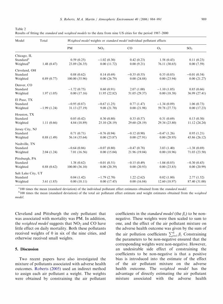
Table 2 contains the results of fitting the modelsto the data from each city. This table contains theindividual pollutant effects obtained from thestandard model and the weights assigned to eachpollutant and the estimated effect of this airpollutant mixture obtained from the weighted

model.The weighted model produces more interpretable

and parsimonious results than the standard model

because the weighted model assigns weights to eachair pollutant and pollutants attracting weight closeto 0 can be ignored. For example, in Chicago thestandard model suggests that increments in theconcentration of PM, CO, O2 and SO2 will result

ARTICLE IN PRESS

Table 1

Results of simulations comparing the standard and weighted models

Total Weighted model weights or standard model individual pollutant effects

PM NO2 CO O3 SO2

Actuala 0.00 20.00 20.00 20.00 20.00 20.00

sb 0.00 (0.79) 0.02 (0.27) 0.01 (0.42) 0.00 (0.31) 0.00 (0.45) �0.04 (0.29)

wc 0.00 (0.57) 18.26 (27.08) 19.28 (31.96) 17.82 (28.00) 22.84 (31.82) 21.80 (30.94)

Actual 0.75 33.33 33.33 33.33 0.00 0.00

s 0.70 (0.81) 0.24 (0.30) 0.23 (0.39) 0.24 (0.33) �0.05 (0.46) 0.04 (0.31)

w 0.90 (0.36) 28.12 (27.18) 19.01 (27.69) 29.57 (27.33) 8.90 (18.35) 14.40 (21.86)

Actual 1.25 20.00 20.00 20.00 20.00 20.00

s 1.29 (0.79) 0.31 (0.27) 0.19 (0.45) 0.29 (0.33) 0.24 (0.41) 0.27 (0.28)

w 1.31 (0.36) 23.96 (20.79) 19.63 (23.94) 22.38 (18.16) 14.39 (18.70) 19.63 (17.58)

Actual 1.50 33.33 33.33 33.33 0.00 0.00

s 1.52 (0.74) 0.52 (0.29) 0.52 (0.36) 0.48 (0.30) 0.02 (0.40) �0.01 (0.27)

w 1.63 (0.34) 30.37 (17.39) 27.50 (21.29) 31.62 (18.88) 5.72 (11.37) 4.80 (9.27)

Actual 2.50 20.00 20.00 20.00 20.00 20.00

s 2.57 (0.78) 0.53 (0.28) 0.48 (0.41) 0.50 (0.32) 0.55 (0.42) 0.52 (0.29)

w 2.51 (0.47) 21.4 (12.42) 20.50 (17.45) 20.49 (12.01) 17.14 (14.74) 20.47 (11.70)

Actual 3.00 33.33 33.33 33.33 0.00 0.00

s 2.93 (0.79) 1.00 (0.28) 1.02 (0.41) 0.97 (0.34) �0.07 (0.43) 0.01 (0.27)

w 3.02 (0.33) 32.99 (9.42) 29.86 (16.63) 34.24 (13.22) 1.05 (4.53) 1.86 (5.09)

Actual 5.00 20.00 20.00 20.00 20.00 20.00

s 4.96 (0.82) 1.00 (0.27) 0.92 (0.41) 1.07 (0.34) 0.99 (0.45) 0.98 (0.32)

w 4.86 (0.56) 20.95 (6.48) 19.36 (10.90) 22.38 (7.40) 17.13 (10.58) 20.17 (6.89)

Actual 6.00 33.33 33.33 33.33 0.00 0.00

s 6.01 (0.80) 1.97 (0.28) 2.03 (0.41) 1.99 (0.32) 0.03 (0.45) 0.00 (0.31)

w 5.99 (0.31) 32.92 (4.69) 32.51 (9.23) 34.11 (7.29) 0.12 (1.22) 0.34 (1.96)

Actual 10.00 20.00 20.00 20.00 20.00 20.00

s 10.01 (0.81) 2.00 (0.29) 1.96 (0.40) 2.02 (0.33) 2.02 (0.46) 2.01 (0.30)

w 9.95 (0.58) 20.14 (3.12) 19.92 (4.74) 20.31 (3.42) 19.32 (5.35) 20.31 (2.96)

a100 times the actual values of y and ai that were used to generate mortality.b100 times the mean (standard deviation) of the total and individual pollutant effect estimates obtained from the standard model over

200 simulations.c100 times the mean (standard deviation) of the total air pollutant effect estimate and weight estimates obtained from the weighted model

over 200 simulations.

S. Roberts, M.A. Martin / Atmospheric Environment 40 (2006) 984–991988

in increased mortality, while increments in theconcentration of NO2 will result in reduced mortal-ity. On the other hand, the weighted model predictsthat the air pollutant mixture associated withincreases in mortality is made up of approximatelyone part PM to three parts O3, and that NO2, COand SO2 are not associated with mortality. In thisexample, the weighted model provides three benefitsover the standard model. Firstly, the weighted model

avoids the implausible assertion that air pollutantcan have a protective effect. Secondly, the weighted

model assigns three air pollutants weights of 0,indicating that in Chicago these three pollutants are

not associated with increases in mortality. Lastly,the weighted model provides an estimate of the airpollutant mixture that is associated with increases inmortality. These benefits of the weighted model canalso be seen in the results for the other eight cities.

The results for the weighted model reveal inter-esting interpretations from the analysis about theeffects of the five air pollutants on mortality in thenine cities considered. This insight is unavailablefrom the results of the standard model. In all citiesexcept Houston the weighted model suggests that thepollutant mixture associated with daily mortalityconsists only of one or two pollutants. In both

ARTICLE IN PRESS

Table 2

Results of fitting the standard and weighted models to the data from nine US cities for the period 1987–2000

Model Total Weighted model weights or standard model individual pollutant effects

PM NO2 CO O3 SO2

Chicago, IL

Standarda 0.59 (0.25) �1.02 (0.30) 0.42 (0.23) 1.58 (0.43) 0.11 (0.23)

Weightedb 1.48 (0.47) 23.89 (26.35) 0.00 (11.72) 0.00 (9.21) 76.11 (30.65) 0.00 (7.59)

Cleveland, OH

Standard 0.88 (0.62) 0.14 (0.69) �0.35 (0.55) 0.35 (0.85) �0.01 (0.54)

Weighted 0.89 (0.77) 100.00 (35.96) 0.00 (26.79) 0.00 (24.88) 0.00 (23.94) 0.00 (21.27)

Denver, CO

Standard �1.72 (0.75) 0.60 (0.91) 2.07 (1.00) �1.10 (1.05) 0.85 (0.66)

Weighted 1.97 (1.05) 0.00 (17.16) 11.95 (22.82) 51.05 (29.37) 0.00 (18.38) 36.99 (27.41)

El Paso, TX

Standard �0.95 (0.87) �0.67 (1.25) 0.77 (1.47) �1.34 (0.89) 1.06 (0.73)

Weighted �1.99 (1.24) 31.13 (27.19) 9.08 (21.70) 0.00 (21.98) 59.78 (27.73) 0.00 (17.23)

Houston, TX

Standard 0.05 (0.42) 0.30 (0.80) 0.33 (0.57) 0.31 (0.69) 0.13 (0.50)

Weighted 1.11 (0.66) 4.84 (18.89) 25.10 (28.19) 29.60 (28.19) 29.34 (23.80) 11.12 (24.24)

Jersey City, NJ

Standard 0.71 (0.71) �0.76 (0.94) �0.12 (0.90) �0.47 (1.26) 0.95 (1.21)

Weighted 0.88 (1.49) 56.14 (35.64) 0.00 (23.87) 0.00 (27.91) 0.00 (28.95) 43.86 (26.12)

Nashville, TN

Standard �0.64 (0.86) �0.07 (0.80) �0.47 (0.78) 3.03 (1.40) �1.38 (0.69)

Weighted 2.04 (1.24) 7.01 (16.56) 0.00 (15.04) 21.96 (19.04) 0.00 (18.96) 71.03 (23.50)

Pittsburgh, PA

Standard 1.38 (0.62) �0.01 (0.51) �0.15 (0.49) �1.04 (0.85) �0.30 (0.43)

Weighted 0.88 (0.62) 100.00 (36.10) 0.00 (20.39) 0.00 (20.93) 0.00 (23.85) 0.00 (20.99)

Salt Lake City, UT

Standard 0.04 (1.42) �1.79 (2.70) 1.22 (2.62) 0.02 (1.80) 2.77 (1.52)

Weighted 3.61 (1.85) 0.00 (18.11) 0.00 (17.45) 0.00 (16.84) 12.60 (18.97) 87.40 (31.00)

a100 times the mean (standard deviation) of the individual pollutant effect estimates obtained from the standard model.b100 times the mean (standard deviation) of the total air pollutant effect estimate and weight estimates obtained from the weighted

model.

S. Roberts, M.A. Martin / Atmospheric Environment 40 (2006) 984–991 989

Cleveland and Pittsburgh the only pollutant thatwas associated with mortality was PM. In addition,the weighted model suggests that NO2 and CO havelittle effect on daily mortality. Both these pollutantsreceived weights of 0 in six of the nine cities, andotherwise received small weights.

5. Discussion

Two recent papers have also investigated themixture of pollutants associated with adverse healthoutcomes. Roberts (2005) used an indirect methodto assign each air pollutant a weight. The weightswere obtained by constraining the air pollutant

coefficients in the standard model (the bi) to be non-negative. These weights were then scaled to sum toone, and the effect of the air pollutant mixture onthe adverse health outcome was given by the sum of

the air pollution coefficientsPk

i¼1 bi Constraining

the parameters to be non-negative ensured that thecorresponding weights were non-negative. However,an undesirable side effect of constraining thecoefficients to be non-negative is that a positivebias is introduced into the estimate of the effectof the air pollutant mixture on the adversehealth outcome. The weighted model has theadvantage of directly estimating the air pollutantmixture associated with the adverse health

ARTICLE IN PRESSS. Roberts, M.A. Martin / Atmospheric Environment 40 (2006) 984–991990

outcome yet returns an unbiased estimate for theeffect of the air pollutant mixture on the adversehealth outcome. For these reasons the weightedmodel is an improvement over the model developedby Roberts. Hong et al. (1999) used a number of airpollution indices to evaluate the combined effects ofvarious air pollutants. The indices used by Hong etal. were selected a priori and gave each pollutantincluded in the air pollutant index equal weight.This method will perform poorly if the actual airpollutant mixture associated with the adversehealth outcome varies from an equal weighting.The approach proposed here avoids this problem,instead estimating the weights directly fromthe data.

The use of the weighted model in a given locationmay also give rise to other interesting questions thatrequire further investigation such as why in somelocations a pollutant attracted a large weight but inother locations it received an estimated weight of 0.For example, why in Cleveland and Pittsburgh wasPM given a weight of 100% but in Denver, Houstonand Nashville it was given a very small weight?One reason for this result could be that PMhas a different chemical composition in Clevelandand Pittsburgh than in Denver, Houston andNashville. The chemical composition of PM hasalready been investigated in a few air pollutionmortality time series studies (Burnett et al.,2003; Smith et al., 2000a, b). The results from theweighted model could assist and inform suchinvestigations, suggesting in this case that thechemical composition of PM in cities where PM isthe dominant pollutant in the air pollutant mixtureshould be contrasted with the chemical compositionof PM in cities where PM is a minor component ofthe air pollutant mixture.

Instead of investigating the unique effects ofspecific pollutants, it has been suggested that itmight be more reasonable to assume that it is amixture of pollutants that might be consideredharmful to health (Dominici and Burnett, 2003;Moolgavkar, 2003; Stieb et al., 2002). For thesereasons, the development of new models to con-currently estimate the adverse health effects ofmultiple air pollutants has been identified bystatisticians, epidemiologists and policy makers asan important topic of research (Dominici andBurnett, 2003). The weighted model presented here,which provides for identification and estimation of amixture of pollutants associated with adverse healtheffects, is an effective step in this direction.

References

Burnett, R.T., Brook, J., Dann, T., et al., 2003. Association

between particulate and gas phase components of urban air

pollution and daily mortality in eight Canadian cities.

Inhalation Toxicology 12 (Suppl. 4), 15–39.

Chock, D.P., Winkler, S.L., Chen, C., 2000. A study

of the association between daily mortality and ambient

air pollutant concentrations in Pittsburgh, Pennsylvania.

Journal of the Air & Waste Management Association 50,

1481–1500.

Cifuentes, L.A., Vega, J., Kopfer, K., Lave, L.B., 2000. Effect of

the fine fraction of particulate matter versus the coarse mass

and other pollutants on daily mortality in Santiago, Chile.

Journal of the Air & Waste Management Association 50,

1287–1298.

Cox, L.H., 2000. Statistical issues in the study of air pollution

involving airborne particulate matter. Environmetrics 11,

611–626.

Daniels, M.J., Dominici, F., Samet, J.M., Zeger, S.L., 2000.

Estimating particulate matter-mortality dose-response curves

and threshold levels: an analysis of daily time-series for the 20

largest US cities. American Journal of Epidemiology 152,

397–406.

Dominici, F., Burnett, R.T., 2003. Risk models for particulate air

pollution. Journal of Toxicology and Environmental Health-

Part A 66, 1883–1889.

Goldberg, M.S., Burnett, R.T., Valois, M.F., et al., 2003.

Associations between ambient air pollution and daily

mortality among persons with congestive heart failure.

Environmental Research 91, 8–20.

Hong, Y.C., Leem, J.H., Ha, E.H., Christiani, D.C., 1999. PM10

exposure, gaseous pollutants, and daily mortality in Inchon,

South Korea. Environmental Health Perspectives 107,

873–878.

Kelsall, J.E., Samet, J.M., Zeger, S.L., Xu, J., 1997. Air pollution

and mortality in Philadelphia, 1974–1988. American Journal

of Epidemiology 146, 750–762.

Klemm, R.J., Mason Jr., R.M., Heilig, C.M., Neas, L.M.,

Dockery, D.W., 2000. Is daily mortality associated specifically

with fine particles? Data reconstruction and replication

analyses. Journal of the Air & Waste Management Associa-

tion 50, 1215–1222.

Kwon, H.J., Cho, S.H., Nyberg, F., Pershagen, G., 2001. Effects

of ambient air pollution on daily mortality in a cohort of

patients with congestive heart failure. Epidemiology 12,

413–419.

Moolgavkar, S.H., 2000. Air pollution and daily mortality in

three US Counties. Environmental Health Perspectives 108,

777–784.

Moolgavkar, S.H., 2003. Air pollution and daily mortality

in two US counties: season-specific analyses and

exposure–response relationships. Inhalation Toxicology 15,

877–907.

Ostro, B.D., Hurley, S., Lipsett, M.J., 1999. Air pollution and

daily mortality in the Coachella Valley, California: a study of

PM10 dominated by coarse particles. Environmental Re-

search 81, 231–238.

Roberts, S., 2005. A new model for investigating the mortality

effects of multiple air pollutants in air pollution mortality

time series studies, in press.

ARTICLE IN PRESSS. Roberts, M.A. Martin / Atmospheric Environment 40 (2006) 984–991 991

Roemer, W.H., van Wijnen, J.H., 2001. Daily mortality and air

pollution along busy streets in Amsterdam, 1987–1998.

Epidemiology 12, 649–653.

Smith, R.L., Davis, J.M., Sacks, J., Speckman, P., Styer, P.,

2000a. Regression models for air pollution and daily

mortality: analysis of data from Birmingham, Alabama.

Environmetrics 11, 719–743.

Smith, R.L., Kim, Y., Fuentes, M., Spitzner, D., 2000b.

Threshold dependence of mortality effects for fine and course

particles in Phoenix, Arizona. Journal of the Air & Waste

Management Association 50, 1367–1379.

Stieb, D.M., Judek, S., Burnett, R.T., 2002. Meta-analysis of

time-series studies of air pollution and mortality: effects of

gases and particles and the influence of cause of death, age,

and season. Journal of the Air & Waste Management

Association 52, 470–484.

Styer, P., McMillan, N., Gao, F., Davis, J., Sacks, J., 1995. Effect

of outdoor airborne particulate matter on daily death counts.

Environmental Health Perspectives 103, 490–497.

Vedal, S., Brauer, M., White, R., Petkau, J., 2003. Air pollution

and daily mortality in a city with low levels of pollution.

Environmental Health Perspectives 111, 45–51.

Wong, T.W., Tam, W.S., Yu, T.S., Wong, A.H., 2002.

Associations between daily mortalities from respiratory and

cardiovascular diseases and air pollution in Hong Kong,

China. Occupational and Environmental Medicine 59, 30–35.