Investigating the Fundamentals of Swarm Computingevans/theses/persaud.pdf · Investigating the...

Investigating the Fundamentals of Swarm Computing

A Thesis in TCC 402

Presented to

The Faculty of the

School of Engineering and Applied Science University of Virginia

In Partial Fulfillment

of the Requirements for the Degree

Bachelor of Science in Computer Science

by

Ryan K. Persaud

March 27, 2001

On my honor as a University student, on this assignment I have neither given nor received unauthorized aid as defined by the Honor Guidelines for Papers in TCC Courses. ____________________________________________________ Approved _______________________________________________ Technical Advisor - Professor David Evans Approved _______________________________________________

TCC Advisor - Professor W. Bernard Carlson

ii

Abstract

Swarm computing involves devices operating like a swarm of insects. A swarm device is

a small mobile robot with sensing capabilities. Therefore, swarm computing is

significantly different from traditional computing methods in that swarm programs must

be able to handle unknown environments and nodes that are capable of moving. Because

swarm computing differs so drastically from traditional computing, traditional

programming techniques will not work in swarm computing. Before such techniques can

be developed for swarm computing, a better understanding needs to be gained of a swarm

of computing devices. Through experimentation, I sought to gain an understanding of the

basic principles of swarm computing. I used the libraries in the Swarm Development

Group’s package to create multiple programs implementing the same swarm behavior

(primitives). Having wrote these programs, I ran them in the Swarm simulator and

compare characteristics such as the power consumption of nodes. Having completed this

project, I delivered a set of swarm primitives and information that I have gathered on

basic swarm behavior. These primitives are not particularly useful by themselves but

they can be combined and integrated to form swarm applications that actually perform a

useful task. Ideally, other researchers can use my insights to develop future swarm

programs. The researchers can then write programs for swarms of computational devices

to accomplish such tasks as the exploration of Mars, clearing the blockage in arteries or

other tasks that require the coordination of a multitude of devices.

iii

Table of Contents Abstract ...............................................................................................................................ii List of Tables....................................................................................................................... v List of Figures ....................................................................................................................vi 1.0 SWARM COMPUTING NOW AND IN THE FUTURE ...................................... 1

1.1 A Potential Scenario.................................................................................................. 1 1.2 What is Currently Possible........................................................................................ 1 1.3 Definition of Swarm Computing............................................................................... 3 1.4 What is Needed ......................................................................................................... 4 1.5 The Work Done in this Project.................................................................................. 4

2.0 TOOLS USED AND DEFINITION OF PRIMITIVES.......................................... 5

2.1 The Swarm Simulator................................................................................................ 5 2.2 Description of the Cluster and Disperse Primitives .................................................. 6 2.3 Major Difference between Cluster and Disperse ...................................................... 7

3.0 ONE SQUARE AWARE VERSUS TWO SQUARE AWARE............................. 8

3.1 Explanation of structure of Technical Report ........................................................... 8 3.2 Description of how the One Square Aware algorithms were implemented.............. 8 3.3 Description of how the Two Square Aware algorithm was implemented ................ 9

3.3.1 Assumptions made about the devices’ abilities.................................................. 9 3.4 Comparing the Algorithms...................................................................................... 10

3.4.1 Explanation of how Algorithms were Compared............................................. 10 3.4.2 Description of modifications necessary to support movement measurement .. 10 3.4.3 Comparison of Two Square Aware and One Square Aware Algorithms ........ 11

3.5 Analysis of Results.................................................................................................. 11 3.6 Hybrid Implementation of Two Square Aware....................................................... 12

3.6.1 Problem with Two Square Aware Disperse ..................................................... 12 3.6.2 Explanation of Hybrid Disperse Algorithm ..................................................... 13

3.7 Analysis of Hybrid Algorithm................................................................................. 13 4.0 N-SQUARE AWARE ALGORITHM.................................................................. 14

4.1 General Description of Algorithm........................................................................... 14 4.2 Description of how the N-Square Algorithm was Implemented............................. 15

4.2.1 Assumptions..................................................................................................... 15 4.2.2 Modifications to the Base Heatbug Class ........................................................ 16

4.3 Weighting ................................................................................................................ 16 4.4 Result and Analysis of N-Square Algorithm........................................................... 17

4.4.1 Starting Configuration of the Bugs .................................................................. 17 4.4.2 Performance of N-Square Compared to Hybrid and One Square Aware Algorithms:................................................................................................................ 18 4.4.3 Performance of N-Square with 1 <= N <= 4................................................... 19

4.5 Situations where the N-Square algorithm will not terminate:................................. 20 4.6 Computational Issues: ............................................................................................. 21

iv

5.0 THE FUTURE OF MY PRIMITIVES AND SWARM COMPUTING............... 22 5.1 Observations............................................................................................................ 22 5.3 Improvements to my Primitives .............................................................................. 23 5.4 Use of Primitives by Future Researchers ................................................................ 24 5.5 The Future of Swarm Computing............................................................................ 24

Bibliography...................................................................................................................... 26

Works Cited............................................................................................................... 26 References ................................................................. Error! Bookmark not defined.

Appendix A: N-Square Algorithm Implementation.......................................................... 28

v

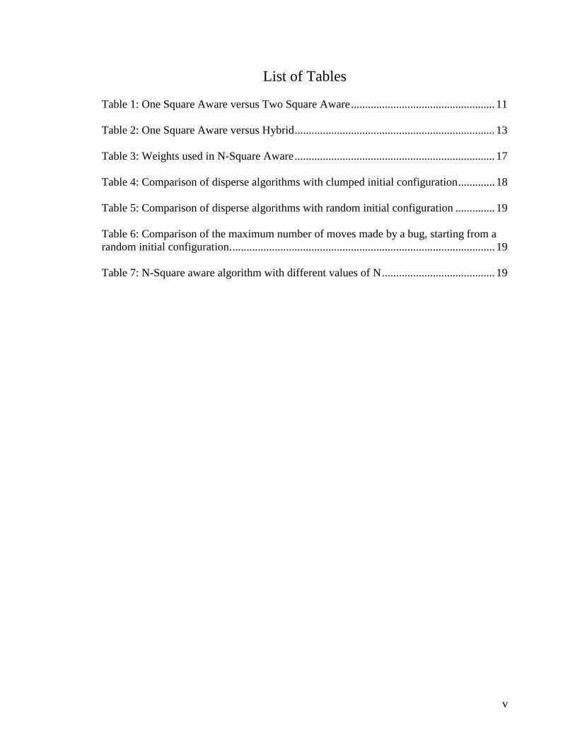
List of Tables Table 1: One Square Aware versus Two Square Aware................................................... 11 Table 2: One Square Aware versus Hybrid....................................................................... 13 Table 3: Weights used in N-Square Aware....................................................................... 17 Table 4: Comparison of disperse algorithms with clumped initial configuration............. 18 Table 5: Comparison of disperse algorithms with random initial configuration .............. 19 Table 6: Comparison of the maximum number of moves made by a bug, starting from a random initial configuration.............................................................................................. 19 Table 7: N-Square aware algorithm with different values of N........................................ 19

vi

List of Figures Figure 1: [1:45].................................................................................................................... 3 Figure 2: Sensing in the 2-Square Aware Algorithm........................................................ 10 Figure 3: Sample square grids........................................................................................... 12 Figure 4: A bug and its candidate squares........................................................................ 14 Figure 5: Evaluation of candidate squares 1 and 3............................................................ 14 Figure 6: Evaluation of a candidate square adjacent to a wall .......................................... 15 Figure 7: Clumped initial configuration versus random initial configuration .................. 18

1

1.0 SWARM COMPUTING NOW AND IN THE FUTURE 1.1 A Potential Scenario

In December of 1999, the Mars Polar Lander was supposed to land on the surface

of Mars and analyze the soil at the South Pole. NASA scientists believe that a

malfunctioning sensor caused the lander to miscalculate its altitude and crash into the

surface. The failure of one sensor caused the failure of a $165 million project [7].

In the future, instead of deploying a solitary unit to survey a planet or other

inaccessible area, a multitude of devices might be employed. These devices would be

rather small in size, but they would have locomotion, sensing and significant processing

capabilities. Furthermore, they would be able to communicate and coordinate their

activities to maximize the use of their resources (power being the most important). For

example, if one device detected an area of interest, it could signal others in its area to

assist it in investigating the region. Another important advantage that this solution has

over the single lander is that even if some devices fail, the remaining units can still

accomplish the mission’s goals.

1.2 What is Currently Possible

While current hardware technology allows for the construction of devices similar

to those mentioned above, the software does not yet exist to coordinate these devices.

For example, in “Next Century Challenges: Mobile Networking for ‘Smart Dust,’” Kahn,

et. al. discuss how sensors and the corresponding signal processing circuitry can be

embedded onto a device that is less than a cubic millimeter.

2

The Smart Dust project is essentially a group of microsensors that report their

readings to a Base-Station Transceiver or BTS. In the simplest situation, the pieces of

dust (nodes) simply relay the information they collect to the BTS using lasers. The

primary problem with this method is that it depends on line-of-sight, so if a node can’t

see the BTS, it will be unable to transmit its data. The Smart Dust devices are currently

unable to move themselves around like the devices in my scenario; however, there are

still similarities. For example, Kahn, et. al. describe a scenario where the Smart Dust

model changes from a group of autonomous sensors to a collection of coordinated

groups. Instead of each “dust particle” having multiple sensors, each device will

specialize and call on the other particles when needed. The main problem inherent in this

scenario is communication between nodes. If a node wants to communicate with another

one, it can attempt to send its message to the BTS and have it act as a relay.

Unfortunately, if the sending node cannot see the BTS, there is no way for the message to

be delivered. Kahn et al believe that the solution to this problem is to implement a

multihop system where the message is either passed to the BTS or to the destination

node. Because of the dynamic nature of the dust’s operating environment and the fact

that links between nodes are not necessarily bi-directional or symmetric, conventional

routing methods will not work with smart dust. New routing algorithms are being

constructed that work with asymmetric links, but none are being developed that consider

unidirectional links [5:277].

3

1.3 Definition of Swarm Computing

The cost of microelectronic mechanical components has decreased to the point

where they can be placed on the same chip with microprocessors and communication

Figure 1: [1:45]

devices [2:74]. As Figure 1 indicates, it is projected that only 150 million of the 8-billion

microcontroller solutions produced in the year 2000 will be used in traditional computers

[1:45]. As more and more devices are equipped with microcontrollers and sensors, a new

class of computational devices will emerge. These devices fall into a class of computing

sometimes referred to as swarm computing, because they operate in a manner that can be

likened to a swarm of insects. The devices exploring Mars in my scenario are an

example of a swarm.

4

1.4 What is Needed

Swarm computing is significantly different from traditional computing methods in

that swarm programs must be able to handle unpredictable physical environments and

execute on nodes that move. Consequently, many of the techniques used to create and

verify traditional programs will not work in swarm computing. Techniques that are

applicable to swarm computing can begin to be developed once the behavior of a swarm

of computing devices is better understood.

1.5 The Work Done in this Project

The main objective of this project was to write and understand the properties of

swarm primitives (basic swarm behaviors). Most of these primitives have analogs in the

insect world such as swarm (all the nodes going in one direction) and cluster (all the

nodes gathering together).

5

2.0 TOOLS USED AND DEFINITION OF PRIMITIVES

2.1 The Swarm Simulator

Early on, professor Evans and I considered extending an existing network

simulator to support the functionality necessary to simulate a swarm and to support

visualization. Once I had extended the simulator, I could then write Swarm primitives

and experiment with them. After some further investigation, we decided that modifying

the simulator would entail quite a bit of work and could probably be considered a thesis

project in its own right. Consequently, we decided to use the Swarm Development

Group’s (SDG) Swarm simulator. The Swarm Simulator already has support for

visualization and simulation programs can be written in Java. I have spent the last two

summers programming with Java, so I am comfortable with it. An example program that

came with the simulator referred to the nodes in the simulator as bugs, and Professor

Evans and I have begun to call the nodes bugs too. Throughout this paper, when I use the

term bug, I mean a node. One characteristic of SDG’s simulator that should be noted is

the way that the bugs execute. A list of the bugs is maintained and this list is iterated

through with each bug’s action function being called. This means that in the simulator

the bugs execute sequentially instead of simultaneously as they would in reality. It would

be too difficult for me to modify the simulator to model simultaneous execution, and for

my purposes sequential execution should be sufficient.

6

2.2 Description of the Cluster and Disperse Primitives

The disperse primitive is where all the nodes in the simulation attempt to situate

themselves so that they are not adjacent to any other nodes. In the context of the swarm

simulator, adjacent means any square that is touching the square in question.

Here is the generalized pseudocode for disperse: DisperseProgram(swarm){

if is_Dispersed(swarm)done

elseDisperse(swarm)

} is_Dispersed(swarm) {

for all bugsif bug has neighbors

return falsereturn true

}

Disperse(swarm) {for all bugs

if bug has neighborsmove()

}

The cluster primitive is essentially the opposite of disperse. Each node attempts to situate

itself so that it is adjacent to at least one other node. The pseudocode for cluster is very

similar to disperse’s:

ClusterProgram(swarm){if is_Clustered(swarm)

doneelse

Cluster(swarm)}

7

is_Clustered(swarm) {

for all bugsif bug has no neighbors

return falsereturn true

}

Cluster(swarm) {for all bugs

if bug has no neighborsmove()

} The only portion of the code that is variable is the implementation of the move function.

In this project, I have basically written different implementations of the move function

and examined their behavior.

2.3 Major Difference between Cluster and Disperse

While Cluster and Disperse may seem very similar, there is one major difference

that makes Disperse more difficult to implement. In Cluster, once a bug has moved

adjacent to another bug, it will never move again. In Disperse, however, a bug may

satisfy the disperse criteria and stop moving, but at some later time be forced to move

again by another bug moving adjacent to it.

8

3.0 ONE SQUARE AWARE VERSUS TWO SQUARE AWARE

3.1 Explanation of structure of Technical Report

In undertaking this project, the direction that I took was often dictated by the

results of the current code I was working on. Consequently, I decided that it made more

sense to present the description of algorithms and their results together instead of putting

them in separate chapters.

3.2 Description of how the One Square Aware algorithms were

implemented

When I first started to work with the Swarm simulator, I wanted to try and write a

simple implementation of a primitive in order to familiarize myself with the package. A

popular example swarm application (for the Java version) is the Heatbug simulation.

Basically, each bug is represented by an instance of a class. These instances are

maintained in a linked list in an ObserverSwarm. The ObserverSwarm constantly iterates

over the list and calls each bug’s Action function. In the standard Heatbug simulation,

the map that the bugs reside on has heat values assigned to each grid location. When a

bug’s action function is invoked, it moves so that it minimizes its heat. The first

modification that I made was to remove all heat considerations from the action function.

For the disperse primitive, I modified the code so that if a bug was adjacent to the current

bug, the current bug moved randomly to an open adjacent location (if possible). For the

cluster primitive, I modified the code so that if the current bug was not adjacent to any

other bugs, the current bug moved randomly to an adjacent location.

9

3.3 Description of how the Two Square Aware algorithm was

implemented 3.3.1 Assumptions made about the devices’ abilities

After implementing the One Square algorithms and viewing their performance, I

began to think of ways to enhance their efficiency. This led me to develop a set of

assumptions about the bugs. The first assumption that I made is that the bugs have the

ability to “sense” what is around them. This assumption was actually used in the One

Square Aware implementations of disperse and cluster. If the bugs did not have the

ability to sense, they would not know when they satisfied the criteria of the respective

primitives. The next assumption that I made is that moving a bug is more expensive than

having the bug do a computation. This means that an extra computation would usually be

preferred to an extra move.

3.3.2 Modifications to the Heatbug Class

The Two Square Aware algorithms assume that the bugs have the ability to sense

any square that can be reached in two moves. This means that the bugs can see further in

the diagonal directions (NE, SW, etc.) than in the regular directions (N, S, etc.). This

may seem odd at first, but there is no way to ensure that a circular area is sensed.

Squares are atomic, and you either see all of one or none of it. As long as the current bug

is not adjacent to any other bugs (first level sensing), the Two Square Aware cluster

algorithm checks the second level of squares in every direction, and moves the bug in the

first direction that has a bug in its second square (see Figure 2). For the Two Square

Aware disperse algorithm, I tried a similar tactic: the first two squares in every direction

10

were checked, and the bug was moved in the first direction that did not have a bug in its

squares. This implementation had some problems that will be discussed in a later section.

Pass 1

bug Pass 2

Figure 2: Sensing in the 2-Square Aware Algorithm 3.4 Comparing the Algorithms 3.4.1 Explanation of how Algorithms were Compared

After I developed the Two Square algorithms, I needed some means to compare

their efficiency to that of the One Square ones. I decided to use the total amount of

moves made by the bugs as my primary metric. As previously mentioned, movement is

assumed to be the main consumer of power. The amount of power that processing and

communication consume is negligible when compared with movement.

3.4.2 Description of modifications necessary to support movement measurement I wanted an overall view of the efficiency of the algorithm, so I decided to

aggregate the movement of all the individual bugs into one variable. This idea lent itself

well to a static class variable in the Bug class. Each time a bug makes a move, it

increments the class variable. Also, every time a bug makes a move, the value of this

variable is displayed to the console.

11

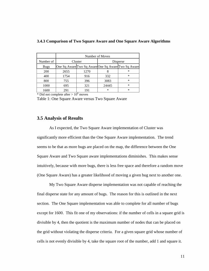
3.4.3 Comparison of Two Square Aware and One Square Aware Algorithms

Number of Moves Number of Cluster Disperse

Bugs One Sq Aware Two Sq Aware One Sq Aware Two Sq Aware200 2655 1270 8 * 400 1754 916 332 * 800 755 396 3083 *

1000 695 321 24445 * 1600 291 191 * *

* Did not complete after > 106 moves Table 1: One Square Aware versus Two Square Aware

3.5 Analysis of Results

As I expected, the Two Square Aware implementation of Cluster was

significantly more efficient than the One Square Aware implementation. The trend

seems to be that as more bugs are placed on the map, the difference between the One

Square Aware and Two Square aware implementations diminishes. This makes sense

intuitively, because with more bugs, there is less free space and therefore a random move

(One Square Aware) has a greater likelihood of moving a given bug next to another one.

My Two Square Aware disperse implementation was not capable of reaching the

final disperse state for any amount of bugs. The reason for this is outlined in the next

section. The One Square implementation was able to complete for all number of bugs

except for 1600. This fit one of my observations: if the number of cells in a square grid is

divisible by 4, then the quotient is the maximum number of nodes that can be placed on

the grid without violating the disperse criteria. For a given square grid whose number of

cells is not evenly divisible by 4, take the square root of the number, add 1 and square it.

12

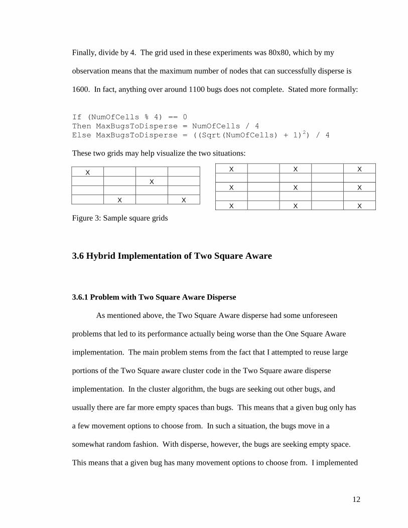
Finally, divide by 4. The grid used in these experiments was 80x80, which by my

observation means that the maximum number of nodes that can successfully disperse is

1600. In fact, anything over around 1100 bugs does not complete. Stated more formally:

If (NumOfCells % 4) == 0Then MaxBugsToDisperse = NumOfCells / 4Else MaxBugsToDisperse = ((Sqrt(NumOfCells) + 1)2) / 4

These two grids may help visualize the two situations:

X X X X

Figure 3: Sample square grids 3.6 Hybrid Implementation of Two Square Aware

3.6.1 Problem with Two Square Aware Disperse

As mentioned above, the Two Square Aware disperse had some unforeseen

problems that led to its performance actually being worse than the One Square Aware

implementation. The main problem stems from the fact that I attempted to reuse large

portions of the Two Square aware cluster code in the Two Square aware disperse

implementation. In the cluster algorithm, the bugs are seeking out other bugs, and

usually there are far more empty spaces than bugs. This means that a given bug only has

a few movement options to choose from. In such a situation, the bugs move in a

somewhat random fashion. With disperse, however, the bugs are seeking empty space.

This means that a given bug has many movement options to choose from. I implemented

X X X X X X X X X

13

the checking of the various directions in a switch statement in the bug class. Since the

bugs had so many options, they were all choosing the first case. This led to all the bugs

moving in the same direction in an approximation of the swarm algorithm.

3.6.2 Explanation of Hybrid Disperse Algorithm

As the name indicates, the hybrid disperse algorithm combines elements of the

One Square Aware algorithm and the Two Square Aware algorithm. First the directly

adjacent squares are scanned. If there is a bug next to the current bug, a direction is

chosen at random, and if the two squares in that direction are clear, the bug will move. If

either square is not clear, another direction is chosen at random. This process of

choosing random directions continues for a fixed number of iterations.

Number of Moves

Number of Disperse Bugs One Sq Hybrid 200 68 99 400 332 283 800 3083 3679 1000 24445 23001 1600 * *

* Did not complete after > 106 moves Table 2: One Square Aware versus Hybrid 3.7 Analysis of Hybrid Algorithm

The hybrid implementation is slightly more efficient than the One Square Aware

implementation in most cases. I would like to develop an aware disperse algorithm that

has the same kind of performance improvement that the Two Square Aware cluster

algorithm has.

14

4.0 N-SQUARE AWARE ALGORITHM 4.1 General Description of Algorithm

Based upon the observations that I made while writing and experimenting with

the Two Square Aware algorithm, Professor Evans and I came up with a more general

algorithm – the N-Square Aware Algorithm. N-Square is similar to the Two Square

algorithm, with the primary difference being that each square surrounding a given

location is fully evaluated; that is all of its surroundings are checked.

2 3 4 1 Bug 5 8 7 6

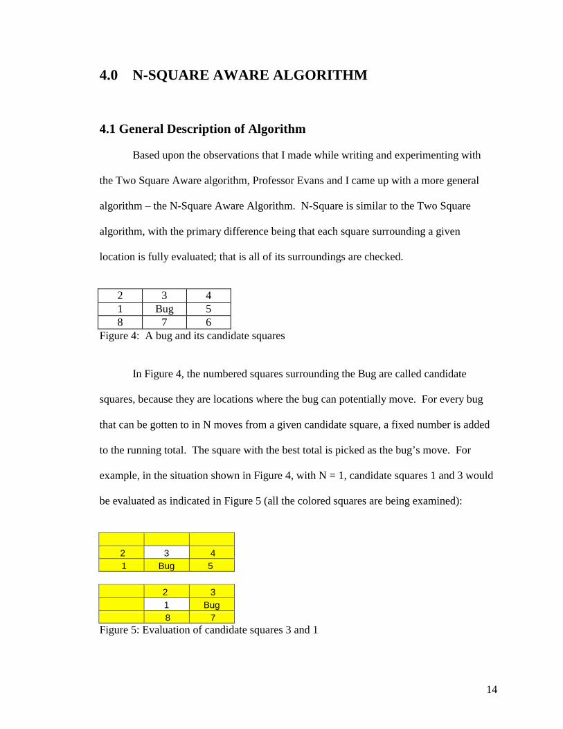
Figure 4: A bug and its candidate squares

In Figure 4, the numbered squares surrounding the Bug are called candidate

squares, because they are locations where the bug can potentially move. For every bug

that can be gotten to in N moves from a given candidate square, a fixed number is added

to the running total. The square with the best total is picked as the bug’s move. For

example, in the situation shown in Figure 4, with N = 1, candidate squares 1 and 3 would

be evaluated as indicated in Figure 5 (all the colored squares are being examined):

2 3 4 1 Bug 5

2 3 1 Bug 8 7

Figure 5: Evaluation of candidate squares 3 and 1

15

N can be set to different values to increase the sensing radius of the algorithm. Setting N

to a value higher than 1 does not mean that only squares at radius N are examined. All

radii from 1 to N are considered and added to a square’s running total. Here is the

pseudocode for the N-Square algorithm:

move(Square,N) {for currSquare = all the candidate squares of Square

for radius = 1 to Ncheck for bugs radius away from currSquareincrease currSquare’s score by # bugs found

move to candidate square with the best score}

4.2 Description of how the N-Square Algorithm was Implemented 4.2.1 Assumptions

Several assumptions were necessary in translating the N-Square algorithm from

pseudocode to Java code that would work in the Swarm simulator. These assumptions

are mainly due to the fact that a Swarm map is a finite environment (like the real world).

The first assumption necessary was that a wall does not count as a bug and therefore does

not affect a location’s running total. Next, a location’s total will be calculated using all

valid locations; that is, out of range locations will not be considered.

3 4 5 2 A 6 1 8 7

Figure 6: Evaluation of a candidate square adjacent to a wall In Figure 6, the thick black vertical line represents a wall. Only squares 4, 5, 6, 7 and 8

will be used to determine the score for candidate square A. Squares 1, 2 and 3 (which do

16

not actually exist) will not be used. This assumption brings up the issue of weighting,

which will be discussed in Section 4.3.

4.2.2 Modifications to the Base Heatbug Class

The implementation of the N-Square algorithm required significant modifications

to the base Heatbug class. Because there were many possible situations for a bug to be in

(in a corner, against the wall, in the middle of the map, etc.), it was necessary to add

functions to calculate the number of bugs in a given direction (top, bottom, left, right and

diagonals). Additionally, a function had to be added that could determine which

combination of the directional functions needed to be called for a given bug. A fairly

involved function was also added to maintain scoring information for each possible

candidate square of the current bug. While I was testing the N-Square algorithm, I

noticed that it was exhibiting swarm behavior. This behavior was subtler than in the Two

Square Aware disperse, but it was still noticeable that the bugs were favoring the lower

left direction and congregating in that area of the map. I applied what I learned in writing

the Two Square Aware algorithm, and selected a location at random if several locations

had the same score. The Java code for the N-Square algorithm can be found in Appendix

A.

4.3 Weighting

After the initial implementation of the N-Square Aware algorithm, it became

evident that some form of weighting would be necessary. Because the same number of

locations is not checked for all candidate locations, it is necessary to normalize each

17

location’s score by dividing by the number of locations actually examined. In Figure 6,

the score for square A with N=1 is divided by 5 before being added to the running total.

It also became evident, that for all N greater than 1, additional weighting is

necessary. As N increases, locations further and further away from the bug are being

considered, and the values obtained in these iterations should affect the totals less and

less. I initially (somewhat naively) believed that a single function that dependent upon N

could be used to scale down the weights. After some experimentation and discussion

with Professor Evans, I decided that the ideal weighting for each N would have to be

determined experimentally.

I used the results for when N=1 to determine suitable weightings for the other Ns.

Basically for a given value of N, I attempted to find the weighting that would consistently

outperform the algorithm using lower values of N. For example, for N=2, I determined

that dividing each candidate square’s score by 5 (after normalizing the score by dividing

by the number of squares considered) provided the best results. Therefore whenever

N=2, 1/5 is used as the weighting.

N Weight 1 1 2 1/5 3 1/11 4 1/15

Table 3: Weights used in N-Square Aware 4.4 Result and Analysis of N-Square Algorithm 4.4.1 Starting Configuration of the Bugs

18

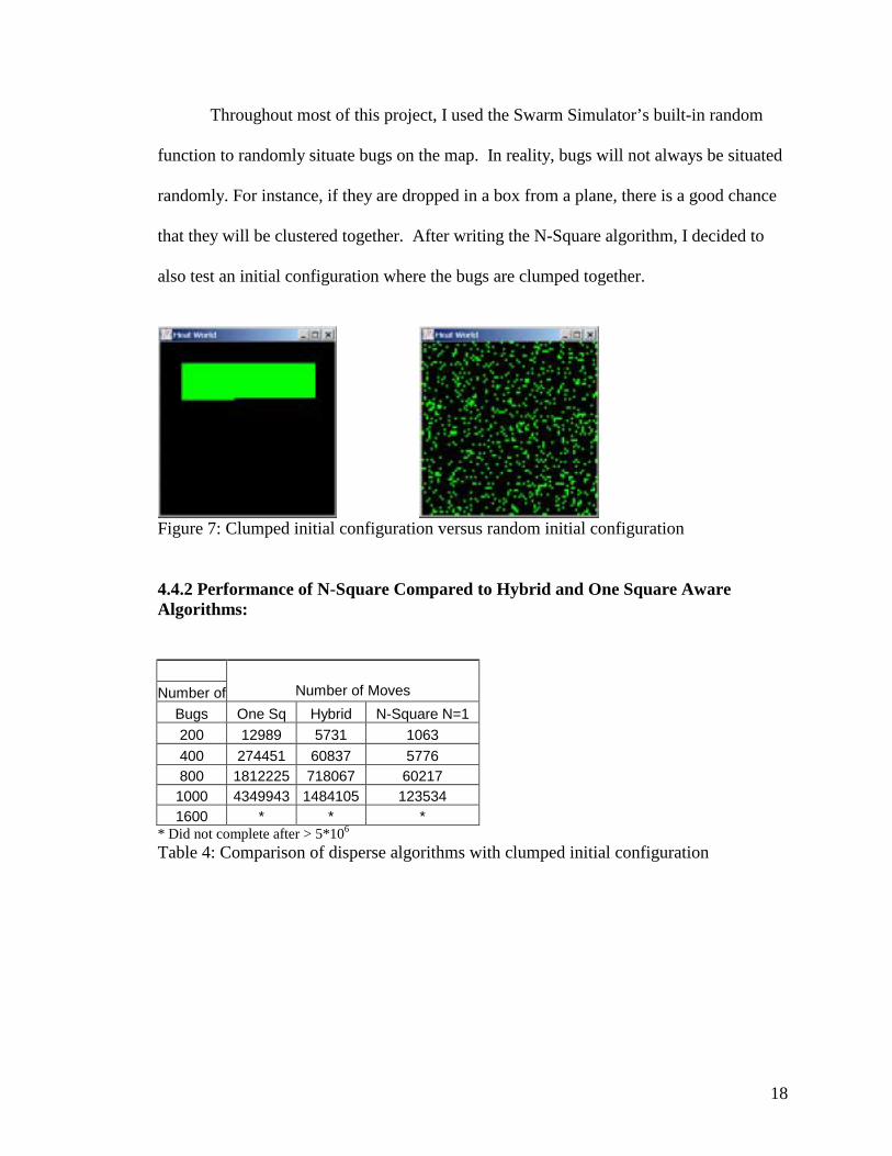
Throughout most of this project, I used the Swarm Simulator’s built-in random

function to randomly situate bugs on the map. In reality, bugs will not always be situated

randomly. For instance, if they are dropped in a box from a plane, there is a good chance

that they will be clustered together. After writing the N-Square algorithm, I decided to

also test an initial configuration where the bugs are clumped together.

Figure 7: Clumped initial configuration versus random initial configuration 4.4.2 Performance of N-Square Compared to Hybrid and One Square Aware Algorithms:

Number of Number of Moves

Bugs One Sq Hybrid N-Square N=1 200 12989 5731 1063 400 274451 60837 5776 800 1812225 718067 60217 1000 4349943 1484105 123534 1600 * * *

* Did not complete after > 5*106

Table 4: Comparison of disperse algorithms with clumped initial configuration

19

Number of Number of Moves

Bugs One Sq Hybrid N-Square N=1 200 68 99 31 400 332 283 112 800 3083 3679 496 1000 24445 23001 1063 1600 * * *

* Did not complete after > 5*106 Table 5: Comparison of disperse algorithms with random initial configuration

Max Number of Move Made by a Bug Number of Cluster Disperse

Bugs One Sq Two Sq One Sq Hybrid N-Square N=1 200 238 121 4 7 1 400 77 53 11 5 2 800 64 24 29 35 3 1000 36 23 88 88 8 1600 19 6 * * *

* Did not complete after > 5*106 Table 6: Comparison of the maximum number of moves made by a bug, starting from a random initial configuration.

As can be seen from the Tables 4, 5 and 6, the N-Square Aware algorithm performs

significantly better than either of the previous algorithms.

4.4.3 Performance of N-Square with 1 <= N <= 4 Number of Number of Moves

Bugs N=1 N=2 N=3 N=4 200 31 31 31 31 400 112 112 113 111 800 496 480 475 466 1000 1063 986 926 939 1600 * * * *

* Did not complete after > 5*106 Table 7: N-Square aware algorithm with different values of N, starting from a random initial configuration

20

Increasing the value of N produced better results from N=1 to N=3, but for N >= 4, the

performance of the algorithm was not consistently better than lower values of N.

4.5 Situations where the N-Square algorithm will not terminate:

When there are many bugs (1200+ in an 80x80 grid), it is possible for a bug to get

“trapped” between other bugs and the wall. The bug will oscillate indefinitely in the area

it is in. A more intelligent weighting system (probably involving giving the walls some

weighting) may prevent this situation from occurring. Additionally, when there are

1200+ bugs, it is possible for two bugs to infinitely rotate around each other. Such

behavior occurs in a region in the middle of symmetrically situated bugs as shown in

Figure 8. This is because the squares in the region always have a lower score than the

squares that lie between the other bugs (these in-between squares are the “escape route”

that the bugs need to take to get to an area where they can properly disperse). This

problem is far more evident for values of N>1.

Figure 8: A situation where two bugs rotate around each other indefinitely Another situation where the algorithm will not terminate is when there are more bugs

than can successfully disperse for a given map size.

21

4.6 Computational Issues:

As the value of N gets larger and larger, the algorithm will obviously take longer

and longer to complete (assuming that this is possible). In calculating the scores for

various scores, there is a significant amount of overlap in the regions that are examined.

By taking advantage of this overlap, the N-Square algorithm could be significantly

optimized.

22

5.0 THE FUTURE OF MY PRIMITIVES AND SWARM COMPUTING

5.1 Observations

The principle that was evident throughout this project is that increasing the local

area examined by a bug provides better global results. In Table 1, the Two Square

Algorithm that examines squares further away than the One Square Algorithm provides

better Cluster results. Also, in table Tables 4 and 5, the N-Square Algorithm provides

much better results than the One Square and Hybrid Algorithms. Furthermore, as seen in

Table 7, increasing the value of N in the N-Square Algorithm (increasing the area

examined) also yields increasingly better results. After a certain point, however,

increasing the area examined no longer reduces the moves that the algorithm makes. In

fact, the performance of the algorithm might actually worsen. An example of this can be

seen in Table 7 with N=4. Additionally, as N increases, the amount of squares that must

be investigated increases by 8N, and the algorithm performs slower and slower.

In implementing the Two Square Algorithm and the N-Square Algorithm, I also

noticed that randomness is useful. When bugs must choose their action from a list of

options (a switch statement for example) and many of the options are valid, a large

number of the bugs will choose the same one. In such a situation, undesirable swarming

behavior (many bugs moving in one direction) will result. By having bugs randomly

choose from the list of valid options, swarm behavior can be avoided.

Throughout this project, I was constantly made aware of the difficulty involved in

predicting swarm behavior. When I implemented the Two Square Aware Disperse, I was

fairly confident that I would have an algorithm that outperformed the One Square Aware.

23

I did not at all expect to end up with a pseudo-swarming primitive. Later, when I

implemented the N-Square Aware algorithm, I expected the efficiency to increase with N

at least to values of 10. Instead, I saw a drop-off in efficiency at the low value of N=4.

Regardless of the weight used, the N-Square algorithm with N=4 cannot consistently

outperform the N=3 version.

5.3 Improvements to my Primitives

Throughout the course of this project, Professor Evans and I thought of many

improvements that could be made to my primitives, but due to time constraints many of

these were not implemented. The most important improvement that can be made is the

ability to pass messages between bugs. With message passing, primitives such as cluster

and disperse can be implemented without assuming sensing capabilities. I made some

attempts to implement a type of simple broadcasting between bugs, but my solution

involved bugs activating each other’s member functions, and it was not a very natural or

clean implementation. Additionally, I was not sure how to represent the direction where

a message was originating.

With the addition of broadcast capabilities, it would also be useful to have some

means to measure time. Bugs could assign timestamps to the messages they receive from

other bugs and use them to determine which message to give the most priority to. This

might require a modification of the Swarm simulator, because currently all the bugs

execute sequentially.

Walls are not given any weight in the N-Square algorithm, and I believe this lead

to some situations where a bug moves indefinitely in a region between bugs and a wall.

24

If the walls had weight, then the bug might be forced to move out of the area they are

oscillating in.

5.4 Use of Primitives by Future Researchers

The primitives I wrote in the course of this project provide little use by

themselves. However, future researchers can use the primitives developed in this project

to create more complicated swarm programs for applications such as the planetary

exploration scenario I presented earlier.

Another use of the primitives by researchers is to experimentally gather data that

will allow them to create formal mathematical models about swarm computing. The

observations I have made in this project are general empirical observations that are not

rigorous. Having formal mathematical models will aid in the development of swarm

applications.

5.5 The Future of Swarm Computing

Several long-term positive impacts are also possible due to the size and

intelligence of a swarm. Nanotechnology is already being applied to medicine, and the

addition of swarm technology would allow for the robots to work closely together for a

common objective, such as clearing blockage in an artery. Another potential application

is exploration. In the past, robots have been used to explore areas that were either too

dangerous or too distant for humans. In most cases a solitary robot would be deployed;

however, as evidenced by the lost Mars’ Polar Lander, this method is not very fault

tolerant. If instead, a swarm of robots was used, the area could be surveyed intelligently

25

and with a higher chance of success. That is, the mission could still be completed

successfully even with some of the robots failing. Professor Evans also sees the methods

used in governing a swarm’s behavior as having applications in the field of e-commerce.

Computerized agents who essentially represent a consumer in his online transactions

have to be able to coordinate their efforts. [3:3]

26

Bibliography

Works Cited 1. Tennenhouse, David. (2000). Embedding the Internet: Proactive Computing.

Communications of the ACM, 43, 44-50. 2. Abelson, Harold, Don Allen, Daniel Coore, Chris Hanson, Erik Rauch, Gerald Jay

Sussman, and Ron Weiss. (2000). Amorphous Computing. Communications of the ACM, 43, 74-82.

3. Evans, David. (2000). Programming the Swarm 4. Kahn, J. M., Katz R. H., & Pister, K. S. J. (1999). Next century challenges: mobile

networking for Smart Dust. Proceedings of the fifth annual ACM/IEEE international conference on Mobile computing and networking, Seattle, WA, August 15-19, 1999 (pp. 271-278). Seattle: ACM.

5. Joshi, Anupam. (2000). On Mobility and Agents. In S. Rajasekaran, P. Pardalos, &D.

F. Hsu, (Eds.), Mobile Networks and Computing (pp. 161-170). Providence, R.I.: American Mathematical Society.

6. Flinn, J., & Satyanarayanan, M. (1999) PowerScope: A Tool for Profiling the Energy

Usage of Mobile Applications. In K. Kelly (Ed.), Second IEEE Workshop on Mobile Computing Systems and Applications, New Orleans, LA, February 25-26, 1999 (pp 2-10). Los Alamitos:IEEE Computer Society.

7. O’Brien, Miles. (1999, December). Scientists continue attempts to contact Mars Polar

Lander as hopes fade. CNN. Retrieved March 14, 2001 from the World Wide Web: http://www.cnn.com/1999/TECH/space/12/08/mars.review/

Additional Works Consulted Estring, D., Govindan, R., Heidemann, J., & Kumar, S. (1999). Next century challenges:

scalable coordination in sensor networks. Proceedings of the fifth annual ACM/IEEE international conference on Mobile computing and networking, Seattle, WA, August 15-19, 1999 (pp. 271-278). Seattle: ACM.

Satyanarayanan, M. (1996). Fundamental challenges in mobile computing. Proceedings

of the fifteenth annual ACM symposium on Principles of distributed computing, Philadelphia, PA, May 23-26, 1996 (pp. 1-7). Philadelphia: ACM.

Li, Q., & Rus, D. (2000). Sending messages to mobile users in disconnected ad-hoc

wireless networks. Proceedings of the sixth annual international conference on

27

Mobile computing and networking, Boston, MA, August 6-11, 2000 (pp. 44-55). Boston: ACM.

Lu, S., & Bharghavan, V. (1996). Adaptive resource management algorithms for indoor

mobile computing. Conference proceedings on Applications, technologies, architectures, and protocols for computer communications, Palo Alto, CA, August 28-30, 1996 (pp. 231-242). Palo Alto: ACM.

28

Appendix A: N-Square Algorithm Implementation public class Heatbug {

//moves this bug has madepublic int locmoves = 0;//maximum amount of moves any bug has madepublic static int locmax = 0;//number of square examined in a given iterationpublic int squares = 0;//total amount of moves made by the swarmpublic static int moves = 0;//spatial coordinatespublic int x, y;//size of the worldpublic int worldXSize, worldYSize;

//Calculates the weighting of the bottom portion of the squaresurrounding a

//candidate squarepublic int Bottom(int a, int b, int n) {

int sum = 0;int start = a - (n - 1);int stop = a + (n - 1);if (start < 0)

start = 0;if (stop > worldXSize)

stop = worldXSize;for (int j = start; j <= stop; j++) {

if (world.getObjectAtX$Y (j, b + n) != null)sum += bugValue;

squares++;}return sum;

}

//Calculates the weighting of the left portion of the squaresurrounding a

//candidate squarepublic int Left(int a, int b, int n) {

int sum = 0;int start = b - (n - 1);int stop = b + (n - 1);if (stop > worldYSize)

stop = worldYSize;if (start < 0)

start = 0;for (int k = start; k <= stop; k++) {

if (world.getObjectAtX$Y (a - n, k) != null)sum += bugValue;


}

29

//Calculates the weighting of the right portion of the squaresurrounding a

//candidate squarepublic int Right(int a, int b, int n) {

int sum = 0;int start = b - (n - 1);int stop = b + (n - 1);if (start < 0)

start = 0;if (stop > worldYSize)

stop = worldYSize;for (int k = start; k <= stop; k++) {

if (world.getObjectAtX$Y (a + n, k) != null)sum += bugValue;


}

//Calculates the weighting of the upper-left corner of the squaresurrounding

//a candidate squarepublic int LeftTop(int a, int b, int n) {

int sum = 0;if (world.getObjectAtX$Y (a - n, b - n) != null)

sum += bugValue;squares++;return sum;

}

//Calculates the weighting of the upper-right corner of the squaresurrounding

//a candidate squarepublic int RightTop(int a, int b, int n) {

int sum = 0;if (world.getObjectAtX$Y (a + n, b - n) != null)


}

//Calculates the weighting of the lower-left corner of the squaresurrounding

//a candidate squarepublic int LeftBottom(int a, int b, int n) {

int sum = 0;if (world.getObjectAtX$Y (a - n, b + n) != null)


}

//Calculates the weighting of the lower-right corner of the squaresurrounding

//a candidate squarepublic int RightBottom(int a, int b, int n) {

int sum = 0;

30

if (world.getObjectAtX$Y (a + n, b + n) != null)sum += bugValue;

squares++;return sum;

}

//Determines which regions of the square surrounding a candidatesquare should

//be investigated and determines the total weight for the candidatesquare

public int GetWeight(int a, int b, int n) {squares = 0;if (world.getObjectAtX$Y (a, b) != null) {

return -100000;}int length = 8*n;int sum = 0;int wallvalue = 0;if ((b - n) > 0)

sum += Top(a,b,n);else

sum += wallvalue;if ((a - n) > 0)

sum += Left(a,b,n);else

sum += wallvalue;if ((a + n) < worldXSize)

sum += Right(a,b,n);else

sum += wallvalue;if ((b + n) < worldYSize)

sum += Bottom(a,b,n);else

sum += wallvalue;if (((b - n) > 0) && ((a - n) > 0))

sum += LeftTop(a,b,n);else

sum += wallvalue;if (((a + n) < worldXSize) && ((b - n) > 0))

sum += RightTop(a,b,n);else

sum += wallvalue;if (((b + n) < worldYSize) && ((a + n) < worldXSize))

sum += RightBottom(a,b,n);else

sum += wallvalue;if (((a - n) > 0) && ((b + n) < worldYSize))

sum += LeftBottom(a,b,n);else

sum += wallvalue;return sum/squares;

}

//determines the best movepublic void makeMove() {

int max = -100000;int Weights[] = {0,0,0,0,0,0,0,0};

31

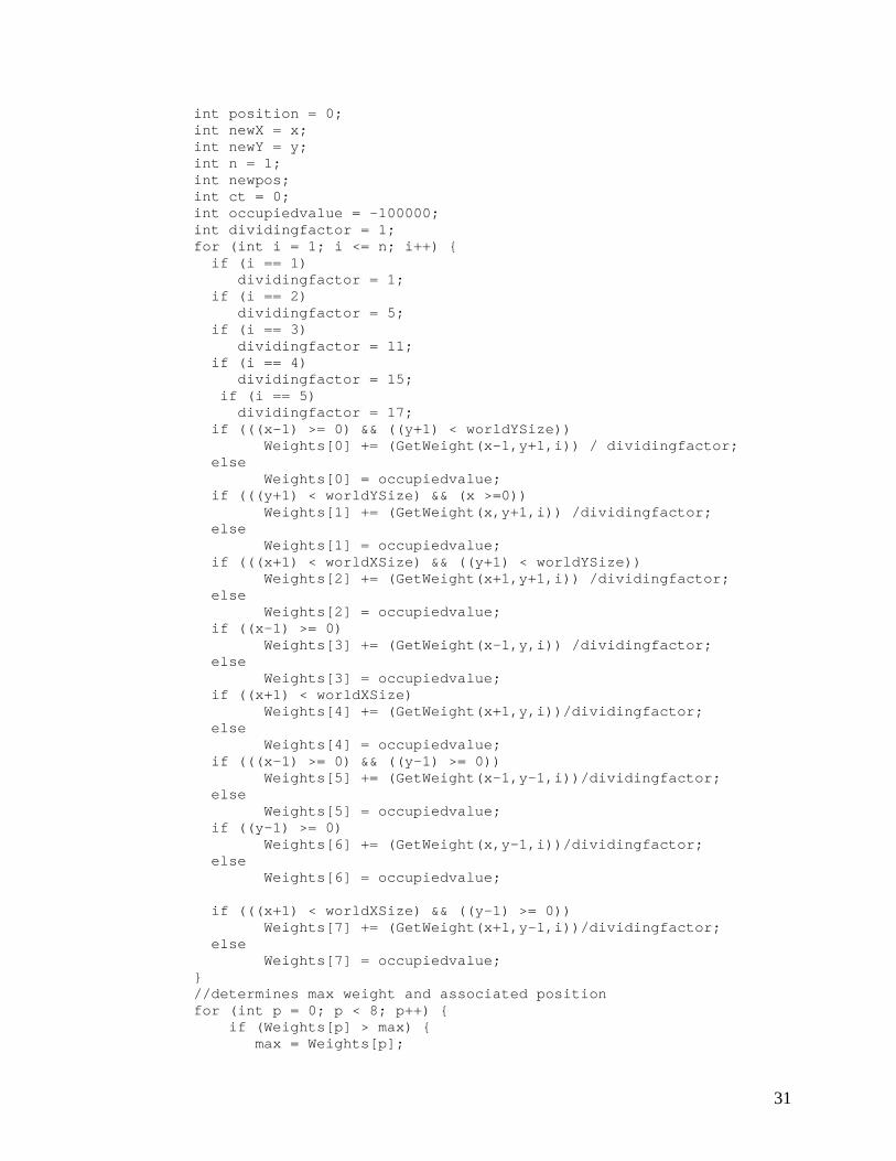
int position = 0;int newX = x;int newY = y;int n = 1;int newpos;int ct = 0;int occupiedvalue = -100000;int dividingfactor = 1;for (int i = 1; i <= n; i++) {

if (i == 1)dividingfactor = 1;





if (((x-1) >= 0) && ((y+1) < worldYSize))Weights[0] += (GetWeight(x-1,y+1,i)) / dividingfactor;

elseWeights[0] = occupiedvalue;

if (((y+1) < worldYSize) && (x >=0))Weights[1] += (GetWeight(x,y+1,i)) /dividingfactor;


if (((x+1) < worldXSize) && ((y+1) < worldYSize))Weights[2] += (GetWeight(x+1,y+1,i)) /dividingfactor;


if ((x-1) >= 0)Weights[3] += (GetWeight(x-1,y,i)) /dividingfactor;


if ((x+1) < worldXSize)Weights[4] += (GetWeight(x+1,y,i))/dividingfactor;


if (((x-1) >= 0) && ((y-1) >= 0))Weights[5] += (GetWeight(x-1,y-1,i))/dividingfactor;


if ((y-1) >= 0)Weights[6] += (GetWeight(x,y-1,i))/dividingfactor;


if (((x+1) < worldXSize) && ((y-1) >= 0))Weights[7] += (GetWeight(x+1,y-1,i))/dividingfactor;


}//determines max weight and associated positionfor (int p = 0; p < 8; p++) {

if (Weights[p] > max) {max = Weights[p];

32

position = p;}

}//determines if more than one position has the max weightint temp[] = new int[8];int tempsize = 0;for (int r = 0; r < 8; r++) {

if (Weights[r] == max) {temp[tempsize] = r;

tempsize++;}

}

//randomly selects from equally weighted positionsif (tempsize > 1) {

position = temp[Globals.env.uniformIntRand.getIntegerWithMin$withMax (0, tempsize-1)];

}

//moves bugif (max != -100000) {

switch (position){case 0:

newX = x-1; newY = y+1; // SWbreak;

case 1:newX = x ; newY = y+1; // Sbreak;

case 2:newX = x+1 ; newY = y+1; // SEbreak;

case 3:newX = x-1 ; newY = y; // Wbreak;

case 4:newX = x+1 ; newY = y; // Ebreak;

case 5:newX = x-1 ; newY = y-1; // NWbreak;

case 6:newX = x ; newY = y-1; // Nbreak;

case 7:newX = x+1 ; newY = y-1; // NEdefault:break;

}

moves++;locmoves++;if (locmoves > locmax)

locmax = locmoves;System.out.println(moves);System.out.println(locmax);world.putObject$atX$Y (null, x, y);

33

x = newX;y = newY;world.putObject$atX$Y (this, newX, newY);

}}

public void heatbugStep () {int newX, newY;newX = x;newY = y;

int location, xm1, xp1, ym1, yp1;xm1 = (x - 1);xp1 = (x + 1);ym1 = (y - 1);yp1 = (y + 1);//Ensures that makeMoves is only called if there is a possible

valid moveif (

//case 1(((x == 0) && (y == 0)) && ((world.getObjectAtX$Y (xp1, y) !=

null)|| (world.getObjectAtX$Y (x, yp1) !=

null)|| (world.getObjectAtX$Y (xp1, yp1) !=

null))) ||//case 2

(((y == 0) && (x != 0)) && (x != (worldXSize -1))&& ((world.getObjectAtX$Y (xm1, y) != null)|| (world.getObjectAtX$Y (xm1, yp1) != null)|| (world.getObjectAtX$Y (x, yp1) != null)|| (world.getObjectAtX$Y (xp1, yp1) != null)|| (world.getObjectAtX$Y (xp1, y) != null))) ||

//case3(((y == 0) && (x == (worldXSize -1)))

&& ((world.getObjectAtX$Y (xm1, y) !=null)

|| (world.getObjectAtX$Y (xm1, yp1) != null)|| (world.getObjectAtX$Y (xp1, y) != null))) ||

//case4(((x == (worldXSize-1)) && (y != 0) && (y != (worldYSize-1)))

&& ((world.getObjectAtX$Y (x, ym1) !=null)

|| (world.getObjectAtX$Y (xm1, ym1) != null)|| (world.getObjectAtX$Y (xm1, y) != null)|| (world.getObjectAtX$Y (xm1, yp1) != null)|| (world.getObjectAtX$Y (x, yp1) != null))) ||

//case 5(((x == (worldXSize-1)) && (y == (worldYSize-1)))

&& ((world.getObjectAtX$Y (x, ym1) != null)|| (world.getObjectAtX$Y (xm1, ym1) != null)|| (world.getObjectAtX$Y (xm1, y) != null))) ||

34

//case 6(((y == (worldYSize-1)) && (x != 0) && (x != (worldXSize-1)))

&& ((world.getObjectAtX$Y (xm1, y) != null)|| (world.getObjectAtX$Y (xm1, ym1) != null)|| (world.getObjectAtX$Y (x, ym1) != null)|| (world.getObjectAtX$Y (xp1, ym1) != null)|| (world.getObjectAtX$Y (xp1, y) != null))) ||

//case 7(((x == 0) && (y == (worldYSize-1)))

&& ((world.getObjectAtX$Y (x, ym1) != null)|| (world.getObjectAtX$Y (xp1, ym1) != null)|| (world.getObjectAtX$Y (xp1, y) != null))) ||

//case 8(((x == 0) && (y != 0) && (y != (worldYSize-1)))

&& ((world.getObjectAtX$Y (x, ym1) !=null)

|| (world.getObjectAtX$Y (xp1, ym1) != null)|| (world.getObjectAtX$Y (xp1, y) != null)|| (world.getObjectAtX$Y (xp1, yp1) != null)|| (world.getObjectAtX$Y (x, yp1) != null))) ||

//case 9(((x != 0) && (x != (worldXSize -1)) && (y != 0)

&& (y != (worldYSize -1))) &&((world.getObjectAtX$Y (xm1, y) != null)

|| (world.getObjectAtX$Y (xp1, y) != null)|| (world.getObjectAtX$Y (x, ym1) != null)

|| (world.getObjectAtX$Y (x, yp1) != null)|| (world.getObjectAtX$Y (xm1, ym1) != null)|| (world.getObjectAtX$Y (xm1, yp1) != null)|| (world.getObjectAtX$Y (xp1, ym1) != null)|| (world.getObjectAtX$Y (xp1, yp1) !=

null))))

{makeMove();

}

}

Investigating the Fundamentals of Swarm Computingevans/theses/persaud.pdf · Investigating the...

Documents

Transcript of Investigating the Fundamentals of Swarm Computingevans/theses/persaud.pdf · Investigating the...