INVESTIGATING THE EFFECTS OF CORROSION ON THE FATIGUE

LIFE OF WELDED STEEL ATTACHMENTS

A Thesis

by

JACK WESLEY SOAPE

Submitted to the Office of Graduate Studies of Texas A&M University

in partial fulfillment of the requirements for the degree of

MASTER OF SCIENCE

May 2012

Major Subject: Civil Engineering

Investigating the Effects of Corrosion on the Fatigue

Life of Welded Steel Attachments

Copyright 2012 Jack Wesley Soape

INVESTIGATING THE EFFECTS OF CORROSION ON THE FATIGUE

LIFE OF WELDED STEEL ATTACHMENTS

A Thesis

by

JACK WESLEY SOAPE

Submitted to the Office of Graduate Studies of Texas A&M University

in partial fulfillment of the requirements for the degree of

MASTER OF SCIENCE

Approved by:

Chair of Committee, Peter B. Keating Committee Members, Gary Fry Alan B. Palazzolo Head of Department, John Niedzwecki

May 2012

Major Subject: Civil Engineering

iii

ABSTRACT

Investigating the Effects of Corrosion on the Fatigue

Life of Welded Steel Attachments. (May 2012)

Jack Wesley Soape, B.S., Texas A&M University

Chair of Advisory Committee: Dr. Peter B. Keating

The railroad industry plays a pivotal role in commerce and greatly impacts

America’s economy. With this in mind, they cannot afford downtime or service

interruptions due to bridge or member replacement. Corrosion of bridges causes millions

of dollars each year for the railroad industry in terms of maintenance and inspection.

Since a large number of these bridges are steel and their service life is typically governed

by fatigue of welded details, it is important to determine the interactions of the corrosion

and fatigue mechanisms. While there are differing opinions on the effects of corrosion

on the fatigue life of welded steel attachments, the intent of this research is to

experimentally investigate the relationship between fatigue and corrosion and determine

whether this relationship is beneficial, neutral, or detrimental to the fatigue behavior of

welded attachments.

In order to investigate the effects of corrosion on the fatigue life of welded steel

attachments, a testing methodology simulating the conditions a bridge could be expected

to experience during its service life is established, executed and the results evaluated.

iv

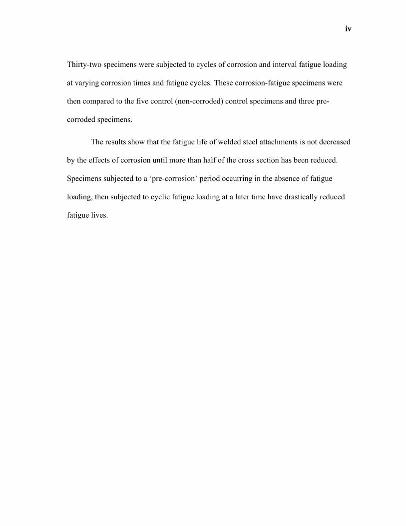
Thirty-two specimens were subjected to cycles of corrosion and interval fatigue loading

at varying corrosion times and fatigue cycles. These corrosion-fatigue specimens were

then compared to the five control (non-corroded) control specimens and three pre-

corroded specimens.

The results show that the fatigue life of welded steel attachments is not decreased

by the effects of corrosion until more than half of the cross section has been reduced.

Specimens subjected to a ‘pre-corrosion’ period occurring in the absence of fatigue

loading, then subjected to cyclic fatigue loading at a later time have drastically reduced

fatigue lives.

v

TABLE OF CONTENTS

Page

ABSTRACT ..................................................................................................................... iii 

TABLE OF CONTENTS ................................................................................................... v 

LIST OF FIGURES .......................................................................................................... vii 

LIST OF TABLES ............................................................................................................. x 

1. INTRODUCTION .......................................................................................................... 1 

1.1 Background .................................................................................................. 1 

1.2 Research Objective ...................................................................................... 2

2. FATIGUE AND CORROSION DAMAGE .................................................................. 3 

2.1 Fatigue .......................................................................................................... 3 

2.2 Corrosion ...................................................................................................... 5 

2.3 Applications ................................................................................................. 9 

2.4 Previous Research ...................................................................................... 11 

2.5 Objective .................................................................................................... 19

3. TESTING PARAMETERS & PROCEDURE ............................................................. 22 

4. RESULTS AND DISCUSSION .................................................................................. 35 

4.1 Fatigue Life ................................................................................................ 35 

4.2 Corrosion Rate ........................................................................................... 44 

4.3 Corrosion Prior to Fatigue Loading ........................................................... 51 

vi

Page

5. LINEAR ELASTIC FRACTURE MECHANICS ....................................................... 56 

6. CONCLUSIONS .......................................................................................................... 64 

7. FURTHER INVESTIGATION .................................................................................... 68 

REFERENCES ................................................................................................................. 70 

VITA ................................................................................................................................ 75 

vii

LIST OF FIGURES

Page

Figure 1. Corrosion Product Deposit .................................................................................. 6 

Figure 2. Surface Corrosion Around Weld ........................................................................ 8 

Figure 3. Initial Corrosion of Mill Scale ............................................................................ 9 

Figure 4. Advanced Corrosion of Mill Scale ..................................................................... 9 

Figure 5. Weathered A588 Weldments ............................................................................ 13 

Figure 6. Weathered A588 Rolled Beams ........................................................................ 15 

Figure 7. Qualitative Diagram of Crack Growth and Corrosion Rate vs. Time .............. 20 

Figure 8. Typical Weld Toe ............................................................................................. 23 

Figure 9. Fatigue Specimen Geometry ............................................................................. 23 

Figure 10. Specimen in Test Frame ................................................................................. 25 

Figure 11. Tensile Test Results ........................................................................................ 26 

Figure 12. S-N Curve for Control Specimens .................................................................. 29 

Figure 13. Specimen Identification .................................................................................. 31 

Figure 14. Stamped Specimen .......................................................................................... 32 

Figure 15. Front of Corrosion Containers ........................................................................ 34 

viii

Page

Figure 16. Back of Corrosion Containers ......................................................................... 34 

Figure 17. S-N Curve for 5%-7 Day Specimens .............................................................. 36 

Figure 18. S-N Curve for 2.5%-7 Day Specimens ........................................................... 36 

Figure 19. S-N Curve for 5%-3.5 Day Specimens ........................................................... 38 

Figure 20. S-N Curve for 2.5%-3.5 Day Specimens ........................................................ 38 

Figure 21. S-N Curve for 1%-3.5 Day Specimens ........................................................... 39 

Figure 22. S-N Curve for 0.5%-3.5 Day Specimens ........................................................ 39 

Figure 23. S-N Curve for All Corrosion-Fatigue Specimens ........................................... 41 

Figure 24. Thru Crack in Specimen 2.5-1 ‘3.5 Day’ (front) ............................................ 42 

Figure 25. Thru Crack in Specimen 2.5-1 ‘3.5 Day’ (back) ............................................ 42 

Figure 26. Fracture Surface of Specimen 5-3 ‘3.5 Day’ at ‘Failure’ ............................... 43 

Figure 27. Fracture Surface of Specimen 5-3 ‘3.5 Day’ at ‘Remaining’ ......................... 44 

Figure 28. 7 Day Corrosion Rate ..................................................................................... 48 

Figure 29. 3.5 Day Corrosion Rate .................................................................................. 49 

Figure 30. Corrosion Damage at Stiffener Termination .................................................. 50 

Figure 31. Corrosion Damage at Root of Weld ............................................................... 50 

Figure 32. Advanced Corrosion led to Fracture at Weld ................................................. 51 

ix

Page

Figure 33. Reduced Cross Section ................................................................................... 53 

Figure 34. S-N Curve for Pre-Corroded & Corrosion-Fatigue Specimens ...................... 53 

Figure 35. Elliptical Surface Crack .................................................................................. 56 

Figure 36. Elliptical Crack Growth .................................................................................. 57 

Figure 37. Crack Growth Rates ........................................................................................ 61 

x

LIST OF TABLES

Page

Table 1. Steel Chemistry and Strength Test Results ........................................................ 27 

Table 2. Control Specimen Fatigue Life .......................................................................... 28 

Table 3. Fatigue Cycle Intervals ...................................................................................... 30 

Table 4. ‘7 Day’ Corrosion-Fatigue Specimens ............................................................... 35 

Table 5. ‘3.5 Day’ Corrosion-Fatigue Specimens ............................................................ 37 

Table 6. ISO Atmospheric Corrosion Category Rates ..................................................... 45 

Table 7. ‘7 Day’ Corrosion Results .................................................................................. 46 

Table 8. ‘3.5 Day’ Corrosion Results ............................................................................... 46 

Table 9. Pre-Corroded Specimens .................................................................................... 52 

Table 10. LEFM Crack Growth Rates ............................................................................. 60 

1

1. INTRODUCTION

1.1 Background

In 2011 the railroad industry invested over $20 billion into our nation’s rail

network. With over 139,000 miles of railroads and nearly 170,000 employees, the

railroads play a pivotal role in not only the American economy but also America’s

productivity (Railroad Infrastructure Investment, 2012). With stakes this high, an

industry cannot afford any downtime or service interruption. By improving the

inspection practices and, in turn, prolonging the service life of bridges, the industry can

better allocate their financial resources to increase overall productivity.

Over the years, our nation’s infrastructure has garnered a great deal of attention

from the public. In 2009 the American Society of Civil Engineers (ASCE) gave the

United States a grade ‘D’ for overall infrastructure and a ‘C’ for bridges (Home: Report

Card for America's Infrastructure, 2011). At a cost of $2.2 trillion over a period of five

years, it would require extensive resources to raise our infrastructure to an acceptable

level. What if the corrosion process was not detrimental to the service life of steel

bridges?

One of the primary design criteria for bridges is fatigue. Fatigue occurs when

cyclical loads cause localized plastic stresses at the tip of an existing flaw or crack.

____________

This thesis follows the style of ASCE: Journal of Structural Engineering.

2

These plastic stresses lead to deformation and damage causing the crack to grow. Abrupt

changes in cross section are significant contributors to increasing the applied stress to the

plastic stress zone by providing a geometric stress concentration. Fatigue design is based

on the severity of the stress concentration induced by changes in cross section and the

respective inherent flaws incurred during the manufacture and fabrication of each

specific condition. With each load cycle the crack grows by an incremental amount

which can ultimately lead to failure.

Previous research programs have tried to determine the relationship between

corrosion and fatigue in steel; all of which have lead to different conclusions. Various

researchers have concluded that the corrosion process decreases the fatigue life of

welded details while others suggested that corrosion can extend the fatigue life.

1.2 Research Objective

The objective of this research program is to validate a testing methodology that

simulates the coupling of the corrosion process with fatigue crack initiation and

propagation. A better understanding of this relationship will provide bridge owners with

better tools to manage the maintenance of bridges as well to operate bridges with

increased reliability in their safety.

3

2. FATIGUE AND CORROSION DAMAGE

2.1 Fatigue

Since the 1950’s, structural engineers have been trying to minimize the effects of

fatigue on steel bridges. Fatigue life is always a concern during the design of a structure

which will see cyclical loads over its lifespan. Fatigue damage occurs when a small flaw

slowly propagates into a crack due to repeated load cycles. Although flaws are not

always visible, they exist in all materials. For bridges, the governing fatigue life is

typically attributed to welded sections. As Fisher et al. (1974) noted, fatigue cracks are

first seen at welds and weld terminations around stiffeners, gusset plates, cover plates, or

other attachments. The fatigue life for welded details is typically governed by the

presence of defects (undercut, slag inclusions, shrinkage cracks, misalignment, etc.),

while the surface defects prove to be the most detrimental to fatigue life. These defects

reside in the stress concentration region of the weld toe and serve as locations for fatigue

crack nucleation (Fisher, Frank, Hirt, & McNamee, 1970).

An initial flaw must experience tensile stresses for a fatigue crack to occur.

During the welding process, regions of high residual tensile stress are created. The

residual stress in these regions can be as high as the tensile yielding stress. These areas

of residual tensile stress are what have caused a higher occurrence of fatigue related

issues in welded construction as compared to riveted construction of the past. Since

weldments have regions of high tensile residual stress, all stress cycles are fully effective

4

in contributing to crack propagation, even if a portion of the stress cycle is compressive.

For the flaw to propagate, the cyclical load must exceed a threshold value. Below this

threshold value, only elastic stresses are experienced at the crack tip, which does not

result in any growth. Above this threshold level, the crack tip develops a plastic stress

region, which causes deformation and leads to the crack growing with each load cycle.

As the crack grows, the net section is decreased, reducing the load carrying capacity and

increasing the overall stress. As the stress increases, the amount of growth occurring

during each successive load cycle increases, leading to exponential growth. The different

category of fatigue details (A, B, C, etc.) as recognized by AISC, AASHTO, etc., are

dependent on the geometric stress risers present at a specific section.

It is very hard to determine the initial flaw size in welds by non-destructive

testing methods. After the completion of fatigue testing, the initial flaw size can be

determined by careful inspection using high magnification microscopes. Since the sizes

can only be known after failure, researchers use various assumptions for initial flaw size

in order to calculate a projected fatigue life. Barsom (1984) found that for category C, D,

and E details the flaws were “equal to or smaller than 0.016 in.” Sakano et al. (1989)

later assumed an initial depth of 20µm (0.000787 in) for estimating the fatigue life.

Although initial flaws may exist, they do not immediately begin to propagate as a

crack with the first cycle experienced. The initial flaws do not contain sharp crack tips

required for crack propagation to occur. Fatigue life is composed of two segments: crack

initiation and crack propagation. For high-cycle fatigue lives, the crack initiation phase

is predominant. The initiation phase is required to transform the radiused root of the

5

initial defect into a sharp crack-like flaw. Numerous researchers have concluded that

approximately 80% of the fatigue life of low stress-high cycle specimens are attributed

to crack initiation.

2.2 Corrosion

ASM (2003) defines aqueous corrosion as “an electrochemical process occurring

at the interface between a material and an aqueous solution.” For this to happen, an

oxidation and reduction (redox) reaction occur at the same time.

The oxidation reaction is the dissolution of the metal and or the formation of

metal oxide, while the reduction reaction is dissolved oxygen reduction. The redox

reaction of iron can be seen in the following equation (ASM, 2003):

2

2 22 2 2 4Fe O H O Fe OH

When the dissolved oxygen in the saltwater reacts with the metallic iron in steel,

the iron is converted to rust. This reaction leads to the iron anode being ‘eaten away’ as

the rust deposit grows (Fisher, Yen, & Wang, 1991). Pitting occurs when a passive film,

such as mill scale, suffers a localized breakdown. This breakdown creates an anode, and

leads to the accelerated dissolution of the underlying metal (ASM, 2003). Figure 1

shows a deposit of corrosion product around a weld toe due to corrosion in an aqueous

environment.

6

Figure 1. Corrosion Product Deposit

During the fabrication and construction phase of a bridge, the steel is either

sandblasted to remove mill scale then painted, or in the case of weathering steel, the mill

scale is removed to allow for ‘uniform’ weathering. Both of these methods are done in

an attempt of corrosion protection. During the life cycle of a bridge, the initial paint

coating will slowly deteriorate and form cracks. If the mill scale is left on, it will also

develop cracks under loading due to its brittle nature. Neither method of surface

treatment is completely successful at mitigating the effects of corrosion.

Similar to fatigue cracks, the corrosion process begins at the surface. Cracks in

the mill scale or paint coating form optimal environments for crevice corrosion and

pitting to take place (Albrecht & Friedland, 1980; Fisher, Kaufmann, & Pense, 1998). In

carbon steel and high-strength low-alloy steel these small surface cracks in the protective

layer (paint or mill scale) lead to an accelerated corrosion rate as compared to a nearby

7

flat area of steel (Fisher, Yen, & Wang, 1991). Even in weathering steels (e.g., ASTM

A588), which are expected to form a protective coating under optimal weathering

conditions, these surface flaws lead to localized pitting as it provides an oxygen deficient

region which acts as the anode for an active corrosion cell (Fisher, Yen, & Wang, 1991).

Since mill scale is cathodic, it is complementary to the anodic region, completing the

corrosion cell (Culp & Tinklenberg, 1980). Since abrupt changes in geometry, such as a

cover plate termination, not only provide a region of stress concentration but can also

make it difficult to apply a protective coating, like paint, these areas tend to show the

first signs of corrosion.

During the welding process the mill scale’s integrity is compromised, due to the

high heat, after which it can easily flake off. As the corrosion mechanism continues, the

affected area will grow outward from the weld. Over time as the corrosion spreads, it

reduces the material thickness as the rust scale flakes away (Culp & Tinklenberg, 1980).

Figure 2 shows the process of corrosion as it spreads from the toe of a weld. The small

crater-like areas seen are individual corrosion cells where the ‘pit’ of the crater is the

local anode.

8

Figure 2. Surface Corrosion Around Weld

Figure 3 shows the effects of corrosion on an unpainted mill scale surface after

15 corrosion cycles of 7 days each in a 3.5% NaCl solution. The areas of bare steel are

where the corrosion process has begun. On the left is a stiffener plate and its weld toe.

The weld toe was the first area to corrode and then began to progress outward. At the

same time, small surface imperfections in the mill scale, which occurred during the

rolling process, begin to corrode. On the far right is the grip section of the specimen. The

tensile grips use a cross hatch pattern to grip the steel which causes breaks in the mill

scale. Figure 4 is a more advanced case of corrosion of mill scale than that of Figure 3.

9

Figure 3. Initial Corrosion of Mill Scale

Figure 4. Advanced Corrosion of Mill Scale

2.3 Applications

Initially, weathering steel was used in bridges because early laboratory testing

showed that under regular wet/dry cycles the high copper content would allow the

formation of a dense outer oxide which would resist future corrosion. In the 1970’s the

Michigan Department of Transportation conducted a study on the effects of corrosion on

weathering steel. Weathering steel had started becoming more prevalent in cases where

10

the bridge would be located over a roadway with high volume traffic below. Due to the

required regular painting of low-alloy steel bridges, it was decided that the additional

initial cost of weathering steel would be more economical than the prohibitive costs of

traffic control associated with the maintenance associated with traditional low-alloy

structural steel (Culp & Tinklenberg, 1980).

It was found that in bridge applications weathering steel was not performing as

expected. Due to Michigan being in a northern climate, deicing salts were used during

the winter months. When weathering steel is contaminated with these salts, the steel

corrodes in the same fashion as traditional non-weathering steels. The salt penetrates the

dense protective oxide and corrodes the material beneath, which forces the protective

oxide layer to rupture as the corrosion product underneath it expands. Initially, the ends

of the bridge girders, which came into contact with supports, were painted in an attempt

to prevent contact with the deicing salts. Upon inspection, it was realized that the middle

section of the bridge girders were exposed to salt contaminated water runoff through

holes in the bridge deck and leaking expansion joints (Culp & Tinklenberg, 1980).

Bridges with and without under-bridge traffic were also subject to airborne salt

contamination. When deicing salts were applied to the roadways, the vehicle traffic

would create a ‘salt cloud,’ which would then settle on the bridge structure. This

occurred regardless of if the bridge structure was above or below the roadway. This

airborne salt contamination even occurred on river crossing bridges (Culp &

Tinklenberg, 1980).

11

Salt contamination was not the sole reason that weathering steels were exceeding

expected corrosion rates. Girder details, such as stiffeners, become catch-alls for dirt and

debris. Upon closer inspection, it was realized that this debris maintained a moist

environment, extending the time of wetness (TOW), which led to extensive corrosion

damage and localized pitting around the detail (Culp & Tinklenberg, 1980).

Since weathering steels are proven to behave comparably to low-alloy steel in the

field, any research regarding the corrosion-fatigue performance of low-alloy steel can be

extrapolated and applied to weathering steels without the need to consider two separate

steel types.

2.4 Previous Research

Throughout the years many well intentioned testing theories have been executed

in attempt to understand the correlation between corrosion and fatigue life. The effects

of corrosion on fatigue life are of importance to many facets of the engineering

community; although there are two sectors from which most of the previous research

was generated: bridge and offshore structures. Unfortunately, none of these testing

theories has recreated an accurate representation of the service conditions bridges

experience.

Albrecht et al. (1983; 1980) conducted a study on small samples and concluded

that if weathering steel were left to weather over a long period of time, the micro-cracks

in the mill scale would lead to crevice corrosion and early crack nucleation. The test

12

specimens were composed of ASTM A588 weathering steel with two welded transverse

stiffeners, which created a Category C detail. The experiment used six stress ranges: 110

MPa, 124 MPa, 144 MPa, 177 MPa, 229 MPa, and 262 MPa (16.0 ksi, 18.0 ksi, 20.9 ksi,

25.6 ksi, 33.2 ksi, and 38.0 ksi). A minimum stress of 3 MPa (0.5 ksi) was used for all

six stress ranges. From a total of 62 specimens, 12 were tested in as-welded condition,

16 were tested after three years of weathering, and 22 were tested after eight years of

weathering. The remaining 12 specimens were weathered for three years, tested to one-

eighth of the average life of the previously tested 3 year weathered specimens, then

weathered for another six months. At the end of six month weathering period, the

specimens were again tested to one-eighth of the average 3 year specimen life. This

cycle of alternate weathering and testing continued until failure.

Testing was conducted on an MTS 89 kN (20 kip) load frame using flat-plate

friction grips. The load was applied as a sinusoidal wave at frequencies ranging from 5

Hz to 10 Hz with a loading rate of 668 kN/sec (150 kip/sec). Albrecht defined failure as

the separation of the sample into two separate pieces.

The specimens were weathered outdoors in University Park, Maryland. Due to

University Park’s proximity to a large metropolitan area, the specimens were exposed to

an above average amount of automobile exhaust. Although the specimens were not

subjected to direct salt contamination or prolonged wet/dry cycles, rust pitting still

occurred. These specimens were tested after three and eight years of weathering and it

was found that they had a reduced fatigue life when compared to the control specimens.

13

The resulting data can be seen in Figure 5 (Albrecht & Friedland, 1980; Albrecht &

Cheng, 1983).

Figure 5. Weathered A588 Weldments

In another study, Albrecht et al. (1994; 2009) conducted an experiment using full

size A588 beams. The beams were blast-cleaned and weathered outdoors. The beams

were weathered in two different fashions, bold exposure and sheltered. During the

weathering process, they were sprayed with a 3% saltwater solution, three times weekly,

50

500

1E+05 1E+06 1E+07

Stress Ran

ge, S

r(M

Pa)

Number of Cycles, N

S‐N Curve: Weathered A588 Weldments

B C D

14

during 3 months of each winter season to simulate contamination by de-icing salts.

During the remainder of the weathering time, the beams were sprayed with plain water

once every 2 weeks.

Three types of beams were tested: built-up welded beams, hot rolled beams, and

hot rolled beams with welded cover plates. Also, three testing environments were used:

air, moist freshwater and moist saltwater. The freshwater and saltwater environments

were applied by using sponges, saturated with their respective solution, during the

testing period. The saltwater solution was composed of 3% sodium chloride dissolved in

freshwater. Failure was defined when at least 50% of the tension flange cracked

(Albrecht & Shabshab, 1994; Albrecht & Lenwari, 2009).

Albrecht found that the corrosion process reduced the fatigue life of welded

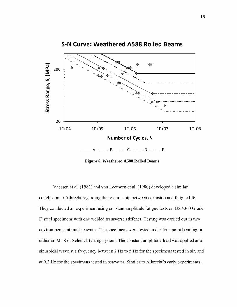
beams, cover-plated beams and hot rolled beams. The results of the hot rolled beam

fatigue testing can be seen in Figure 6. In the sheltered, welded beams, all the cracks

were observed to initiate from rust pits. These results are similar to those of the smaller

weldment samples he tested previously. Since the crevice corrosion and pitting had

already reduced the cross section area, prior to fatigue loading, the results are

understandable (Albrecht & Shabshab, 1994; Albrecht & Lenwari, 2009).

15

Figure 6. Weathered A588 Rolled Beams

Vaessen et al. (1982) and van Leeuwen et al. (1980) developed a similar

conclusion to Albrecht regarding the relationship between corrosion and fatigue life.

They conducted an experiment using constant amplitude fatigue tests on BS 4360 Grade

D steel specimens with one welded transverse stiffener. Testing was carried out in two

environments: air and seawater. The specimens were tested under four-point bending in

either an MTS or Schenck testing system. The constant amplitude load was applied as a

sinusoidal wave at a frequency between 2 Hz to 5 Hz for the specimens tested in air, and

at 0.2 Hz for the specimens tested in seawater. Similar to Albrecht’s early experiments,

20

200

1E+04 1E+05 1E+06 1E+07 1E+08

Stress Ran

ge, S

r(M

Pa)

Number of Cycles, N

S‐N Curve: Weathered A588 Rolled Beams

A B C D E

16

all cracks initiated from locations near the toe of the weld. Vaessen and van Leeuwen

found that the existing design curves were not accurate for projecting the fatigue lives of

welded joints experiencing corrosion by immersion in a seawater environment.

Palin-Luc et al. (2010) conducted testing on low-alloy steel specimens. These

findings also supported those previously found by Albrecht. The test specimens were

made of non-standard hot rolled low-alloy steel, typically used in the manufacture of

mooring chains. Testing was conducted at 20 kHz on an ultrasonic fatigue testing

machine. Three conditions were tested: without corrosion, after pre-corrosion and under

real time artificial seawater flow.

Palin-Luc et al. found that for non-corroded specimens, fatigue cracks

propagated from surface flaws. For the pre-corroded specimens and specimens tested

while immersed, failure occurred due to fatigue cracks propagating from surface

corrosion pits (Palin-Luc, Perez-Mora, Bathias, Dominguez, Paris, & Arana, 2010).

Both Barsom (1984), Out et al. (1984), and Fisher et al. (1991) have proposed

that the corrosion process can be beneficial to the fatigue life. Due to the critical flaws

responsible for fatigue failure of welded details being located on the surface, the

controlling fatigue life is greatly influenced by the stress concentrations welding

typically creates. If the environmental corrosion rate is higher than the crack propagation

rate, the corrosion process could “eliminate or at least decrease the size of the surface

imperfections.” By reducing the flaw size, corrosion would in turn reduce the stress

raiser and prolong the fatigue life (Barsom, 1984).

17

Out et al. (1984) conducted testing on four built-up riveted stringers taken from a

railroad bridge. The bridge from which the stringers originated was 80 years old, and

had considerable signs of corrosion damage. The purpose of the experiment was to

determine the fatigue life of riveted details in high-cycle regions, and determine the

fatigue behavior of built-up members that suffered deterioration, due to corrosion, during

service. The stringers were tested using two Amsler 245 kN (55 kip) hydraulic jacks and

one pulsator in a four-point bending arrangement. The load was applied at a constant

amplitude of 520 cycles per minute (8.67 Hz). Out concluded that if the net cross section

was reduced by more than half due to corrosion, the resulting fatigue life was more

accurately predicted by the next severe detail category. (For example, for the category D

sections that had lost more than half of their area to corrosion, their fatigue life was more

accurately predicted by the design life of category E.)

Waldvogel (1997) conducted testing on the effects of corrosion on the fatigue life

of steel specimens with a machined notch. The specimens were machined into a dog-

bone shape with a 1/32nd of an inch (0.8 mm) groove perpendicular to the direction of

loading. Testing was conducted on an MTS load frame with a nominal stress range of 35

ksi (241.3 MPa) applied as a sinusoidal wave at 20 Hz. Corrosion took place in a 3.5%

sodium chloride solution for a period of either 3.5 days or 7 days, depending on which

exposure group the specimen belonged to. The incremental fatigue loading cycles, of

each load group, were based on 50%, 25%, 12.5% or 6.25% of the average control

specimen fatigue life.

18

After an initial exposure period of seven days for all specimens in the sodium

chloride solution, the specimens were then subjected to their respective incremental

fatigue loading cycles. After the incremental fatigue loading, specimens were returned to

the corrosion solution for another exposure period of either 3.5 days or 7 days. This

sequence of alternating exposure to a corrosive environment and incremental fatigue

loading continued until the specimen failed due to unstable fatigue crack growth. Failure

was defined as the specimen separating into two separate pieces due to fatigue crack

propagation. After each exposure period in the corrosion solution, specimens were

cleaned prior to the incremental fatigue loading. This cleaning process removed the

corrosion product, and allowed for more thickness measurements to be taken, in order to

record the corrosion rate.

Although the data showed that the mean corroded fatigue life exceeded the mean

non-corroded fatigue life, due to the high fatigue cycle intervals which the specimens

experienced, the results were inconclusive in showing a delay in the crack initiation due

to corrosion (Waldvogel, 1997).

The research conducted by Ewalds and Edwards (1982) discussing the effects of

crack closure prevention due to corrosion product wedging, should also be addressed.

The wedging of corrosion product causes a raise in the minimum stress intensity factor.

This change results in the total range of the stress intensity factor, which is the driving

force determining crack growth rates, is decreased. If the stress range intensity factor is

decreased sufficiently, the result can be retardation or even stopping the crack growth.

19

While this phenomena is possible on notched specimens fatigue tested while

submersed in a corrosive solution, this will not occur in the welded details previously

discussed. By testing while the specimen is submersed, it allows for the pumping effect

of the crack displacement to introduce the corrosive solution to the entire depth of the

crack. This does not occur during typical bridge loading as the bridge members are not

submerged and the corrosion occurs on the surface. Without the pumping effect, the

corrosion product cannot develop within the crack, and in turn cause corrosion product

wedging.

Also, welded sections typical to bridges have regions of high residual tensile

stress in the area where the fatigue crack is expected to occur. This region of high

residual tensile stress raises the effective stress range the crack experiences. As the range

of effective stress is raised, the minimum stress value is above the level which could be

affected by corrosion product being present within the crack. Since the crack does not

close due to the residual tensile stresses, the findings of Ewalds and Edwards (1982) is

interesting, but not directly applicable to this research.

2.5 Objective

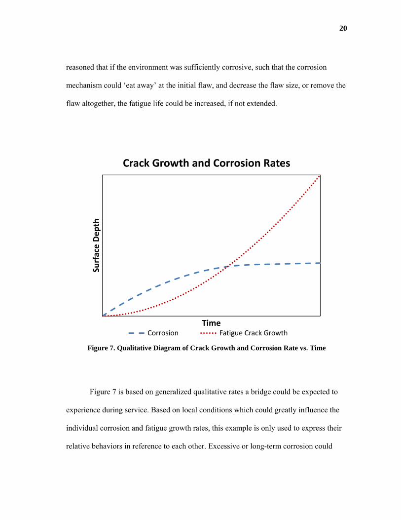
The objective of this research is to show that the corrosion process is not

detrimental to the fatigue life in most cases. Since both the corrosion process and critical

fatigue cracks begin on the surface, it seems logical to deduce that corrosion could in

fact be beneficial to fatigue life. Based on the relationships shown in Figure 7, it can be

20

reasoned that if the environment was sufficiently corrosive, such that the corrosion

mechanism could ‘eat away’ at the initial flaw, and decrease the flaw size, or remove the

flaw altogether, the fatigue life could be increased, if not extended.

Figure 7. Qualitative Diagram of Crack Growth and Corrosion Rate vs. Time

Figure 7 is based on generalized qualitative rates a bridge could be expected to

experience during service. Based on local conditions which could greatly influence the

individual corrosion and fatigue growth rates, this example is only used to express their

relative behaviors in reference to each other. Excessive or long-term corrosion could

Surface Depth

Time

Crack Growth and Corrosion Rates

Corrosion Fatigue Crack Growth

21

result in significant cross section loss causing fracture, or yielding in the event of

overload. This hypothesis is also supported by Fisher et al. (1991) during his field

investigation of riveted bridge members, as well as by Barsom (1984).

The hypothesis that corrosion does not accelerate fatigue crack growth is based

on fracture mechanics. For a fillet weld toe, fatigue failure occurs when surface flaws

develop into unstable cracks. If the corrosion process can slow the development of these

flaws, the fatigue life could be extended.

To test this hypothesis in a laboratory, the typical bridge service life must be

condensed into a reasonable period of time. Although there have previously been studies

conducted on weathering steels (ASTM A588), the current research intends to determine

the effects that corrosion has on the fatigue life of low-alloy structural steel, since the

findings can be applied to weathering steel subject to corrosion due to non-optimal

service environments.

22

3. TESTING PARAMETERS & PROCEDURE

To investigate the effects of corrosion on the fatigue life, the corrosion specimens

were subjected to alternating periods of exposure to a corrosive environment and cyclic

fatigue loading.

The specimens consisted of a 51mm x 3mm x 381mm (2” x 1/8” x 15”) long

main plate, to which one 25.5mm x 13mm x 127mm ( 1” x 1/2” x 5”) longitudinal

stiffener was welded to each side with a 5mm (3/16”) weld. Since the tensile strength

has no relation to the fatigue life, all specimens were created from ASTM A36 bar stock

(Fisher, Frank, Hirt, & McNamee, 1970; Fisher, Albrecht, & Yen, 1974). The welds

were made using a MIG welder with AWS 5.18 ER70S-6 wire. All specimens were

fabricated on the same day by one professional welder to ensure consistency. A typical

weld toe where fatigue cracks are expected to propagate from can be seen in Figure 8.

The dimensions and configuration of the specimens can be seen in Figure 9.

23

Figure 8. Typical Weld Toe

Figure 9. Fatigue Specimen Geometry

24

This AASHTO Category E detail was chosen to provide a lower nominal stress

range, similar to what railroad bridges experience in service, while still having a

reasonably short life cycle. If the nominal stress were, lower it would greatly increase

the fatigue life, and extend the research beyond a reasonable time frame.

All specimens were tested with a stress range (Sr) of 138 MPa (20 ksi), and a

minimum stress (Smin) of 69 MPa (10 ksi). The loading was applied at 30 Hz as a

constant amplitude sinusoidal wave. This loading rate was chosen due to the low stress

range, which would cause a high cycle fatigue life. Had the loading rate been lower,

each testing sequence would have extended beyond a reasonable time frame.

Additionally, the specimens were preloaded to a mean stress of 138 MPa (20 ksi) to

begin testing. The preload was applied to prevent the process variable control (PVC)

function of the testing software from exceeding the maximum stress value during the

first quarter of the sine wave as the load ramps upwards. The servo-hydraulic test frame

used was an MTS Model 312.21, capable of producing 100 kN (22 kips) of force. The

servo-hydraulic test frame was controlled by MTS Basic TestWare software program.

The software was used in its load control mode, which allowed the user to determine the

upper and lower bounds of the sinusoidal load wave. In addition to the applied load

function settings, force and displacement interlocks were utilized to ensure that power

surges or shortages did not influence the results. Since the program was in load control,

the only data that needed to be recorded was cycle count, which was recorded in the test

log. Each specimen had a designated testing and log file that kept a continuous record of

each individual incremental fatigue loading cycle counts, total fatigue cycle counts to

25

date, and any errors encountered (such as the displacement/force interlocks being

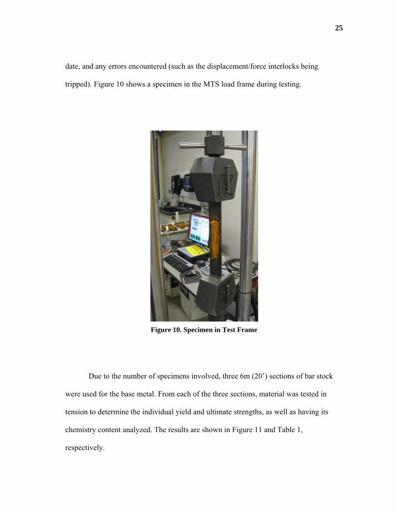
tripped). Figure 10 shows a specimen in the MTS load frame during testing.

Figure 10. Specimen in Test Frame

Due to the number of specimens involved, three 6m (20’) sections of bar stock

were used for the base metal. From each of the three sections, material was tested in

tension to determine the individual yield and ultimate strengths, as well as having its

chemistry content analyzed. The results are shown in Figure 11 and Table 1,

respectively.

26

Figure 11. Tensile Test Results

0

30

60

90

0.0 0.2 0.4 0.6 0.8 1.0 1.2

Stress (ksi)

Displacement (in)

Tensile Strength

Sample A Sample B Sample C

27

Table 1. Steel Chemistry and Strength Test Results

Figure 11 shows that each of the three samples had very similar behavior during

the yield and ultimate strength testing. Based on the similarity of the stress-strain plots of

‘Sample B’ and ‘Sample C’, it is likely that both came from the same stock. While

‘Sample A’ had slightly less elongation prior to failure than the other two samples, all

yield strengths and ultimate strengths are nearly identical. The high yield strength results

of these samples are typical of thin A36 steel plate.

The samples also had very similar chemical content, which can be seen in Table

1. It is obvious that the chemical content meets the minimum ASTM requirements for

A36 steel. It should also be noted that the chemical composition is very similar to the

requirements for weathering steel (A588). Because of this chemical similarity to

weathering steel, the conclusions of this research will be applicable to both weathering

Sample: A B C Weld A36

Carbon 0.2 0.2 0.2 0.091 0.25 (max)

Manganese 0.8 0.77 0.77 1.13

Phosphorus 0.045 0.046 0.046 0.029 0.04 (max)

Sulfur 0.047 0.033 0.034 0.033 0.05 (max)

Silicon 0.18 0.15 0.15 0.61 0.40 (max)

Nickel 0.13 0.12 0.12 0.03

Molybdenum 0.02 0.02 0.02 0.01

Chromium 0.09 0.09 0.09 0.04

Copper 0.56 0.56 0.56 0.36 0.20 (min)

Cobalt 0.011 0.011 0.011 0.005

Tin 0.020 0.018 0.018 <0.005

Fy (ksi) 61 60 60   36 (min)

Fu (ksi) 85 84.5 85 36 (min)

28

and non-weathering steels alike. The consistency of these three samples is beneficial for

this experiment since there are no major variances in the strength or chemical

composition. This consistency allows for a more controlled experiment with less factors

of uncertainty.

Five control specimens were fatigue tested without exposure to a corrosive

environment in order to establish a baseline for the fatigue life. For both the control and

corrosion specimens, failure was defined as the separation of the specimen into two

separate pieces. The results of the control specimen fatigue lives are shown in Table 2,

and plotted with the lower bound design life for AASHTO Category E details in Figure

12.

Table 2. Control Specimen Fatigue Life

Specimen Base Metal Fatigue Life

CS I A 645,244

CS II B 687,437

CS III C 362,802

CS IV C 445,190

CS V A 448,703

518,000Average Life :

29

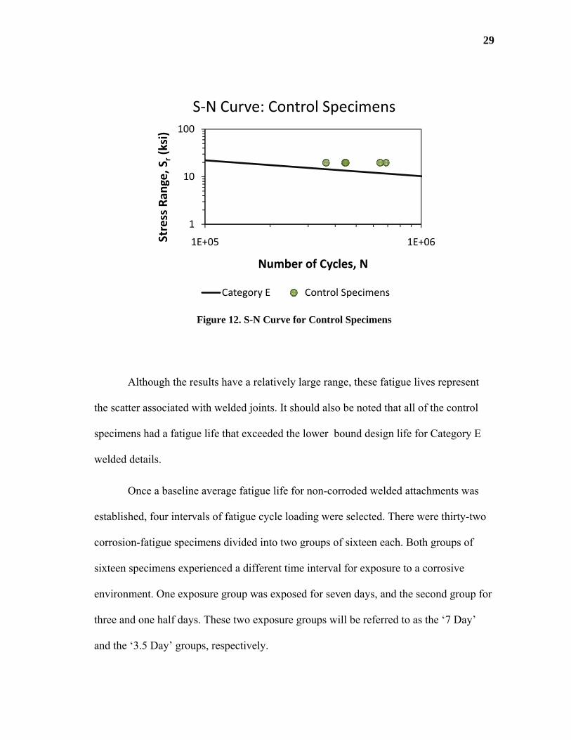
Figure 12. S-N Curve for Control Specimens

Although the results have a relatively large range, these fatigue lives represent

the scatter associated with welded joints. It should also be noted that all of the control

specimens had a fatigue life that exceeded the lower bound design life for Category E

welded details.

Once a baseline average fatigue life for non-corroded welded attachments was

established, four intervals of fatigue cycle loading were selected. There were thirty-two

corrosion-fatigue specimens divided into two groups of sixteen each. Both groups of

sixteen specimens experienced a different time interval for exposure to a corrosive

environment. One exposure group was exposed for seven days, and the second group for

three and one half days. These two exposure groups will be referred to as the ‘7 Day’

and the ‘3.5 Day’ groups, respectively.

1

10

100

1E+05 1E+06Stress Ran

ge, S

r(ksi)

Number of Cycles, N

S‐N Curve: Control Specimens

Category E Control Specimens

30

Each exposure group was tested at the end of its exposure period; after the

incremental fatigue testing, the surviving specimens within the exposure group were

returned to the corrosive environment for their respective exposure times. Prior to each

fatigue testing interval, specimens were individually cleaned under running water with a

nylon brush and steel wool to remove any corrosion scale that had accumulated during

the exposure period. As a result of this cleaning process, the corrosion rate was a linear

function of time, which closely approximates the long-term steady-state corrosion of

bridges. The corrosion process and fatigue loading sequence was repeated until failure.

Each of the two exposure groups were further divided into four groups of four.

These sub-groups would each experience separate fatigue load cycle intervals at the end

of each exposure period. The four fatigue load cycle intervals were determined as a

percentage of the average control specimen fatigue lives (Table 2). Each sub-group’s

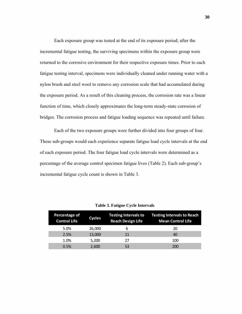
incremental fatigue cycle count is shown in Table 3.

Table 3. Fatigue Cycle Intervals

Percentage of 

Control LifeCycles

Testing Intervals to 

Reach Design Life

Testing Intervals to Reach 

Mean Control Life

5.0% 26,000 6 20

2.5% 13,000 11 40

1.0% 5,200 27 100

0.5% 2,600 53 200

31

From Table 3, it can be seen that the specimen group projected to reach mean

control life first is the 5%-‘3.5 Day’ after 10 weeks, and the last group will be the 0.5%-

‘7 Day’ after 200 weeks.

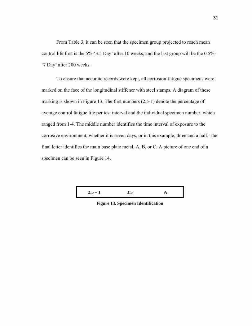
To ensure that accurate records were kept, all corrosion-fatigue specimens were

marked on the face of the longitudinal stiffener with steel stamps. A diagram of these

marking is shown in Figure 13. The first numbers (2.5-1) denote the percentage of

average control fatigue life per test interval and the individual specimen number, which

ranged from 1-4. The middle number identifies the time interval of exposure to the

corrosive environment, whether it is seven days, or in this example, three and a half. The

final letter identifies the main base plate metal, A, B, or C. A picture of one end of a

specimen can be seen in Figure 14.

2.5 – 1 3.5 A

Figure 13. Specimen Identification

32

Figure 14. Stamped Specimen

In addition to the corrosion-fatigue specimens, there were three pre-corroded

specimens. These three specimens were placed into the corrosion solution and did not

experience any interval fatigue loading. The pre-corroded specimens were marked as ‘X-

1’,’X-2’, and ‘X-3’. To maintain similar conditions as the corrosion-fatigue specimens,

the pre-corroded specimens were removed from the corrosion bath and cleaned every

seven days. The pre-corroded specimens were to determine the effect on the fatigue life

of specimens suffering from corrosion cross section loss prior to any cyclic fatigue

loading, similar to the experiments performed by Albrecht (1984).

The corrosion-fatigue specimens were initially placed in the corrosive

environment for seven days prior to the start of the fatigue loading intervals. After this

initial exposure period, each specimen was subjected to its respective fatigue loading

interval, then returned to the corrosive environment for another exposure period (3.5

days or 7 days).

The corrosive environment, that the corrosion-fatigue and pre-corroded

specimens were exposed to, was composed of eight containers which housed the

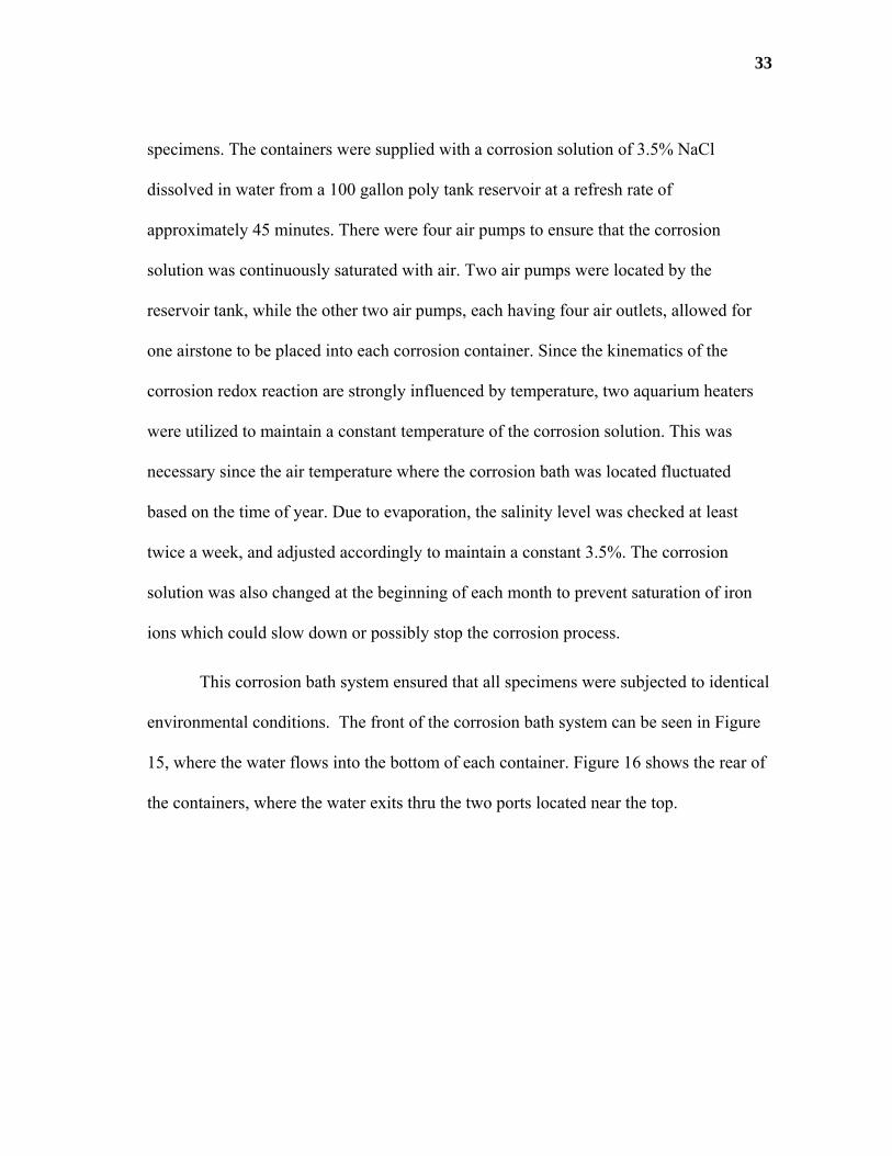
33

specimens. The containers were supplied with a corrosion solution of 3.5% NaCl

dissolved in water from a 100 gallon poly tank reservoir at a refresh rate of

approximately 45 minutes. There were four air pumps to ensure that the corrosion

solution was continuously saturated with air. Two air pumps were located by the

reservoir tank, while the other two air pumps, each having four air outlets, allowed for

one airstone to be placed into each corrosion container. Since the kinematics of the

corrosion redox reaction are strongly influenced by temperature, two aquarium heaters

were utilized to maintain a constant temperature of the corrosion solution. This was

necessary since the air temperature where the corrosion bath was located fluctuated

based on the time of year. Due to evaporation, the salinity level was checked at least

twice a week, and adjusted accordingly to maintain a constant 3.5%. The corrosion

solution was also changed at the beginning of each month to prevent saturation of iron

ions which could slow down or possibly stop the corrosion process.

This corrosion bath system ensured that all specimens were subjected to identical

environmental conditions. The front of the corrosion bath system can be seen in Figure

15, where the water flows into the bottom of each container. Figure 16 shows the rear of

the containers, where the water exits thru the two ports located near the top.

34

Figure 15. Front of Corrosion Containers

Figure 16. Back of Corrosion Containers

35

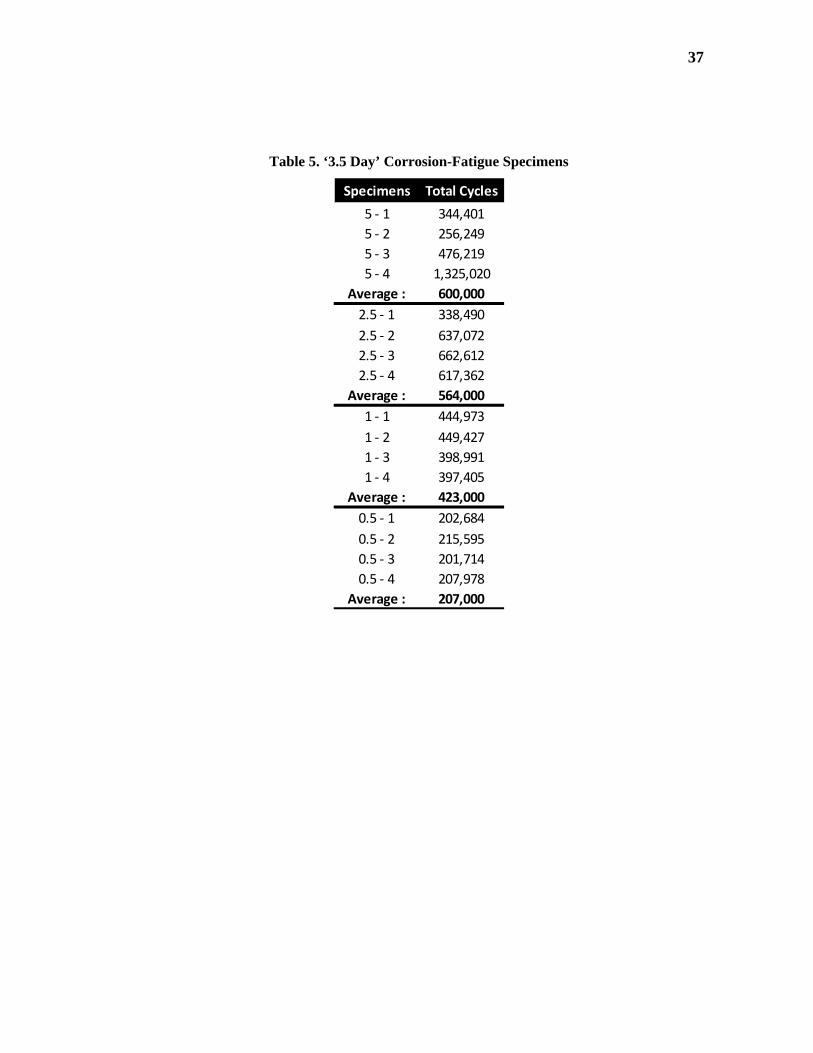
4. RESULTS AND DISCUSSION

4.1 Fatigue Life

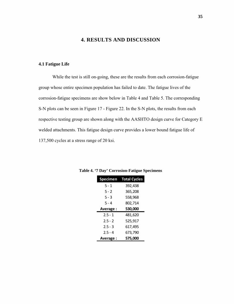
While the test is still on-going, these are the results from each corrosion-fatigue

group whose entire specimen population has failed to date. The fatigue lives of the

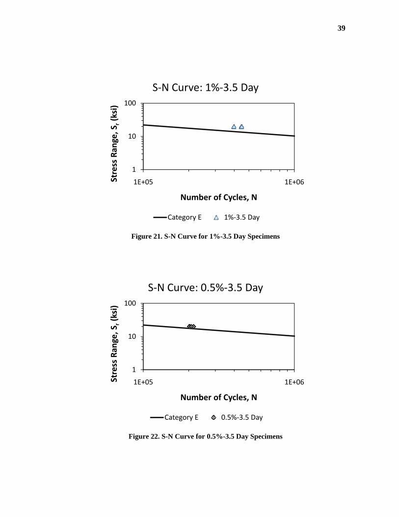
corrosion-fatigue specimens are show below in Table 4 and Table 5. The corresponding

S-N plots can be seen in Figure 17 - Figure 22. In the S-N plots, the results from each

respective testing group are shown along with the AASHTO design curve for Category E

welded attachments. This fatigue design curve provides a lower bound fatigue life of

137,500 cycles at a stress range of 20 ksi.

Table 4. ‘7 Day’ Corrosion-Fatigue Specimens

Specimen Total Cycles

5 ‐ 1 392,438

5 ‐ 2 365,208

5 ‐ 3 558,968

5 ‐ 4 802,714

Average : 530,000

2.5 ‐ 1 481,620

2.5 ‐ 2 525,917

2.5 ‐ 3 617,495

2.5 ‐ 4 673,790

Average : 575,000

36

Figure 17. S-N Curve for 5%-7 Day Specimens

Figure 18. S-N Curve for 2.5%-7 Day Specimens

1

10

100

1E+05 1E+06Stress Ran

ge, S

r(ksi)

Number of Cycles, N

S‐N Curve: 5%‐7 Day

Category E 5%‐7 Day

1

10

100

1E+05 1E+06Stress Ran

ge, S

r(ksi)

Number of Cycles, N

S‐N Curve: 2.5%‐7 Day

Category E 2.5%‐7 Day

37

Table 5. ‘3.5 Day’ Corrosion-Fatigue Specimens

Specimens Total Cycles

5 ‐ 1 344,401

5 ‐ 2 256,249

5 ‐ 3 476,219

5 ‐ 4 1,325,020

Average : 600,000

2.5 ‐ 1 338,490

2.5 ‐ 2 637,072

2.5 ‐ 3 662,612

2.5 ‐ 4 617,362

Average : 564,000

1 ‐ 1 444,973

1 ‐ 2 449,427

1 ‐ 3 398,991

1 ‐ 4 397,405

Average : 423,000

0.5 ‐ 1 202,684

0.5 ‐ 2 215,595

0.5 ‐ 3 201,714

0.5 ‐ 4 207,978

Average : 207,000

38

Figure 19. S-N Curve for 5%-3.5 Day Specimens

Figure 20. S-N Curve for 2.5%-3.5 Day Specimens

1

10

100

1E+05 1E+06Stress Ran

ge, S

r(ksi)

Number of Cycles, N

S‐N Curve: 5%‐3.5 Day

Category E 5%‐3.5 Day

1

10

100

1E+05 1E+06Stress Ran

ge, S

r(ksi)

Number of Cycles, N

S‐N Curve: 2.5%‐3.5 Day

Category E 2.5%‐3.5 Day

39

Figure 21. S-N Curve for 1%-3.5 Day Specimens

Figure 22. S-N Curve for 0.5%-3.5 Day Specimens

1

10

100

1E+05 1E+06Stress Ran

ge, S

r(ksi)

Number of Cycles, N

S‐N Curve: 1%‐3.5 Day

Category E 1%‐3.5 Day

1

10

100

1E+05 1E+06Stress Ran

ge, S

r(ksi)

Number of Cycles, N

S‐N Curve: 0.5%‐3.5 Day

Category E 0.5%‐3.5 Day

40

As seen in Table 5, the fatigue lives of the corrosion-fatigue specimens in groups

‘1%-3.5 Day’ and ‘0.5%-3.5 Day’ showed a decreased fatigue life. This is likely due to

the extent of corrosion damage and the resulting cross section loss. The results are

discussed later in more detail.

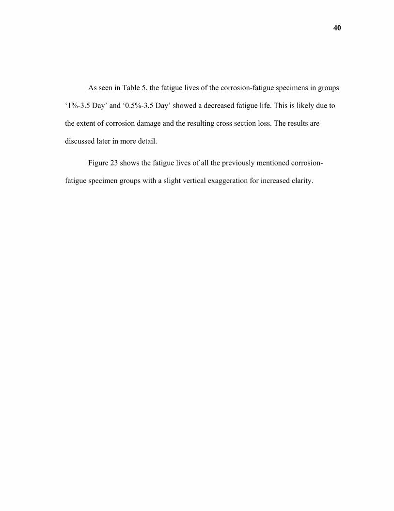
Figure 23 shows the fatigue lives of all the previously mentioned corrosion-

fatigue specimen groups with a slight vertical exaggeration for increased clarity.

41

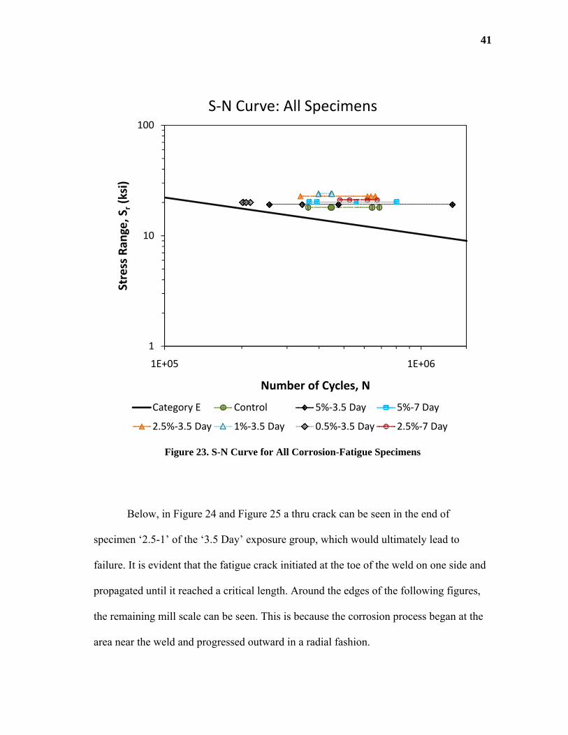
Figure 23. S-N Curve for All Corrosion-Fatigue Specimens

Below, in Figure 24 and Figure 25 a thru crack can be seen in the end of

specimen ‘2.5-1’ of the ‘3.5 Day’ exposure group, which would ultimately lead to

failure. It is evident that the fatigue crack initiated at the toe of the weld on one side and

propagated until it reached a critical length. Around the edges of the following figures,

the remaining mill scale can be seen. This is because the corrosion process began at the

area near the weld and progressed outward in a radial fashion.

1

10

100

1E+05 1E+06

Stress Ran

ge, S

r(ksi)

Number of Cycles, N

S‐N Curve: All Specimens

Category E Control 5%‐3.5 Day 5%‐7 Day

2.5%‐3.5 Day 1%‐3.5 Day 0.5%‐3.5 Day 2.5%‐7 Day

42

Figure 24. Thru Crack in Specimen 2.5-1 ‘3.5 Day’ (front)

Figure 25. Thru Crack in Specimen 2.5-1 ‘3.5 Day’ (back)

43

Figure 26 shows the fatigue fracture surface of the failure end of specimen ‘5-3’

of the ‘3.5 Day’ exposure group. It is a clear example of the incremental damage that

each later fatigue loading interval contributed to the ultimate failure of the specimen.

There are multiple crack initiation sites which can be seen.

Figure 26. Fracture Surface of Specimen 5-3 ‘3.5 Day’ at ‘Failure’

While the specimens can only fail at one end of the welded stiffener, it is very

likely that the remaining weld toe also experienced fatigue crack growth. To investigate,

the remaining weld toe is cut down to size and the base plate is notched along the same

plane as the leading edge of the weld toe. Liquid nitrogen is then used to lower the

sample below its brittle transition temperature, making it easier to fracture the steel

along the failure plane of the crack and the notch. The results of using this technique can

be seen below in Figure 27.

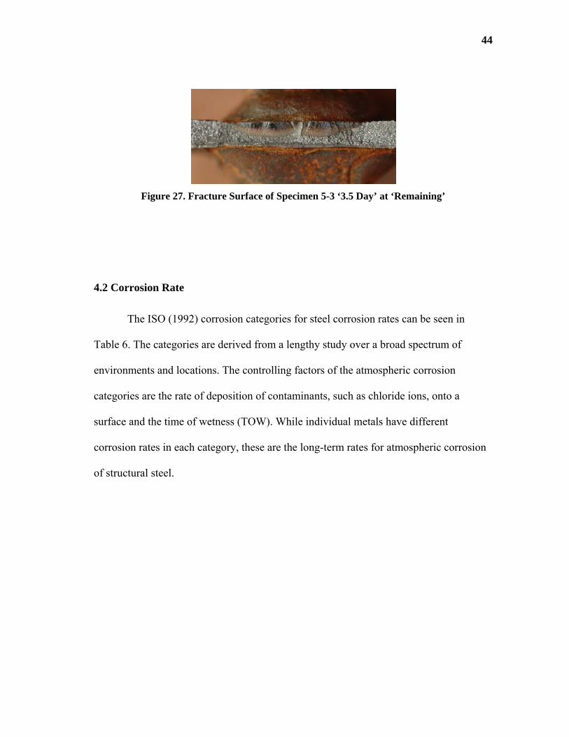
44

Figure 27. Fracture Surface of Specimen 5-3 ‘3.5 Day’ at ‘Remaining’

4.2 Corrosion Rate

The ISO (1992) corrosion categories for steel corrosion rates can be seen in

Table 6. The categories are derived from a lengthy study over a broad spectrum of

environments and locations. The controlling factors of the atmospheric corrosion

categories are the rate of deposition of contaminants, such as chloride ions, onto a

surface and the time of wetness (TOW). While individual metals have different

corrosion rates in each category, these are the long-term rates for atmospheric corrosion

of structural steel.

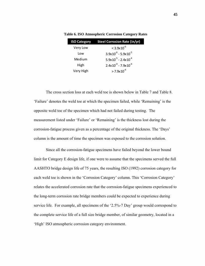
45

Table 6. ISO Atmospheric Corrosion Category Rates

ISO Category Steel Corrosion Rate (in/yr)

Very Low < 3.9x10‐6

Low 3.9x10‐6‐ 5.9x10

‐5

Medium 5.9x10‐5‐ 2.4x10

‐4

High 2.4x10‐4‐ 7.9x10

‐4

Very High > 7.9x10‐4

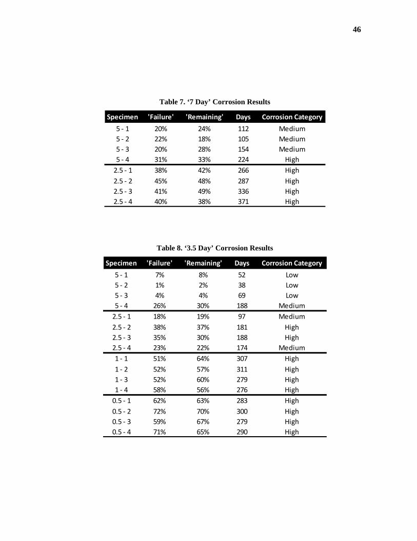
The cross section loss at each weld toe is shown below in Table 7 and Table 8.

‘Failure’ denotes the weld toe at which the specimen failed, while ‘Remaining’ is the

opposite weld toe of the specimen which had not failed during testing. The

measurement listed under ‘Failure’ or ‘Remaining’ is the thickness lost during the

corrosion-fatigue process given as a percentage of the original thickness. The ‘Days’

column is the amount of time the specimen was exposed to the corrosion solution.

Since all the corrosion-fatigue specimens have failed beyond the lower bound

limit for Category E design life, if one were to assume that the specimens served the full

AASHTO bridge design life of 75 years, the resulting ISO (1992) corrosion category for

each weld toe is shown in the ‘Corrosion Category’ column. This ‘Corrosion Category’

relates the accelerated corrosion rate that the corrosion-fatigue specimens experienced to

the long-term corrosion rate bridge members could be expected to experience during

service life. For example, all specimens of the ‘2.5%-7 Day’ group would correspond to

the complete service life of a full size bridge member, of similar geometry, located in a

‘High’ ISO atmospheric corrosion category environment.

46

Table 7. ‘7 Day’ Corrosion Results

Specimen 'Failure' 'Remaining' Days Corrosion Category

5 ‐ 1 20% 24% 112 Medium

5 ‐ 2 22% 18% 105 Medium

5 ‐ 3 20% 28% 154 Medium

5 ‐ 4 31% 33% 224 High

2.5 ‐ 1 38% 42% 266 High

2.5 ‐ 2 45% 48% 287 High

2.5 ‐ 3 41% 49% 336 High

2.5 ‐ 4 40% 38% 371 High

Table 8. ‘3.5 Day’ Corrosion Results

Specimen 'Failure' 'Remaining' Days Corrosion Category

5 ‐ 1 7% 8% 52 Low

5 ‐ 2 1% 2% 38 Low

5 ‐ 3 4% 4% 69 Low

5 ‐ 4 26% 30% 188 Medium

2.5 ‐ 1 18% 19% 97 Medium

2.5 ‐ 2 38% 37% 181 High

2.5 ‐ 3 35% 30% 188 High

2.5 ‐ 4 23% 22% 174 Medium

1 ‐ 1 51% 64% 307 High

1 ‐ 2 52% 57% 311 High

1 ‐ 3 52% 60% 279 High

1 ‐ 4 58% 56% 276 High

0.5 ‐ 1 62% 63% 283 High

0.5 ‐ 2 72% 70% 300 High

0.5 ‐ 3 59% 67% 279 High

0.5 ‐ 4 71% 65% 290 High

47

The cross section loss measurements were taken at approximately 0.2 inches

away from the weld toe at the center of the base metal. This location was chosen in order

to rule out an artificially thin measurement due to material necking, which occurs during

failure. Measurements were taken using a digital Mitutoyo micrometer with 0.050 inch

diameter tips.

In addition to the measurements taken at the weld toe of each specimen, two

coupons from a leftover section base metal ‘A’ were used to approximate the corrosion

rate. The mill scale on each was removed to approximate the conditions around the weld

toe where the mill scale was damaged during the welding processs, as well as to provide

a uniform surface for precise and consistent measurements. Each coupon was then

carefully measured and weighed. After their respective exposure periods, each coupon

was removed, cleaned with a nylon brush and fine steel wool, and measured. The results

can be seen in Figure 28 and Figure 29.

48

Figure 28. 7 Day Corrosion Rate

0

0.2

0.4

0.6

0.8

1

0

0.05

0.1

0.15

0.2

0.25

0.3

0 10 20 30 40 50

gram

s

mm

Time (days)

7 Day Corrosion Rate

Length Loss Width Loss Thickness Loss Weight Loss

49

Figure 29. 3.5 Day Corrosion Rate

These coupon results can only serve as a reference for the corrosion rates

experienced by the corrosion-fatigue test specimens. Since the corrosion coupons were

not loaded and were smaller than the corrosion-fatigue specimens, there will inherently

be some variation in the coupon corrosion rates as compared to that of the corrosion-

fatigue specimens.

Although the extent of corrosion damage on each corrosion-fatigue specimen

varied, Figure 30 shows how aggressive the corrosion process was as the silhouette of

the remaining portion of weld toe can be seen. Figure 31 shows that the corrosion

process has nearly eaten through to the root of the weld. In fact, the stiffener shown in

0

0.2

0.4

0.6

0.8

0

0.05

0.1

0.15

0.2

0.25

0 10 20 30 40

gram

s

mm

Time (days)

3.5 Day Corrosion Rate

Length Loss Width Loss Thickness Loss Weight Loss

50

Figure 31 fell off when liquid nitrogen was used to fracture the remaining weld toe of

the corrosion-fatigue specimen, as previously discussed; the result can be seen in Figure

32.

Figure 30. Corrosion Damage at Stiffener Termination

Figure 31. Corrosion Damage at Root of Weld

51

Figure 32. Advanced Corrosion led to Fracture at Weld

The corrosion results from this research are in line with the findings of Culp and

Tinklenberg (1980). Table 1 shows that the weld metal has a rich chemical composition,

which is similar to that of ASTM A588 weathering steel, yet Figure 30-Figure 32 show

that the weld region corroded as quickly as the base metal. Since it is known that the

field weathering behavior of A588 steel is not as corrosion resistant as initially thought,

the findings of this research will be applicable to carbon steel, high strength low-alloy

steel and weathering steels susceptible to salt contamination (Culp & Tinklenberg,

1980).

4.3 Corrosion Prior to Fatigue Loading

The results of the three pre-corroded specimens that were exposed to the

corrosive environment for 376 days without experiencing any fatigue loading, are shown

below in Table 9 and Figure 33. Prior to their fatigue testing, the three pre-corroded

52

specimens were measured to determine the approximate amount of cross sectional area

lost, and thickness lost at the center of the base plate. All losses are given as percentages

of original dimensions. Figure 34 shows the reduced cross section of the base plate due

to the corrosion process; the white dotted line represents the original section outline.

Table 9. Pre-Corroded Specimens

SpecimenArea Loss at 

Failure Section

Thickness Loss at 

Failure SectionFatigue Life

X‐1 44% 44% 64,147

X‐2 48% 47% 76,559

X‐3 51% 47% 1,252

53

Figure 33. S-N Curve for Pre-Corroded & Corrosion-Fatigue Specimens

Figure 34. Reduced Cross Section

1

10

100

1E+03 1E+04 1E+05 1E+06

Stress Ran

ge, S

r(ksi)

Number of Cycles, N

S‐N Curve: All Specimens

Category E Control 5%‐3.5 Day 5%‐7 Day

2.5%‐3.5 Day 1%‐3.5 Day 0.5%‐3.5 Day 2.5%‐7 Day

X‐1 X‐2 X‐3

54

These results coincide with the findings of Albrecht et al. (1980; 1983) that

weathering prior to fatigue cycling can reduce the fatigue life. By pre-corroding the

specimens prior to any fatigue loading, the location of the most severe stress

concentrations transition from being in the weld region to the most severe case of rust

pitting. This is true for both weathering and non-weathering steels alike. For non-

weathering steel, the net area is also reduced locally (Ref. Table 7 & Table 9) which

causes a reduction in fatigue life.

By comparing the fatigue lives of the pre-corroded specimens with the fatigue

lives of corrosion-fatigue specimens suffering similar cross section loss, it is evident that

the interaction between simultaneous corrosion and cyclic loading improves fatigue life.

This is because corrosion-fatigue specimens, which underwent simultaneous corrosion

and fatigue loading, had much longer fatigue lives with as much, if not more, cross

section loss than the pre-corroded specimens.

Although it is not captured in this study due to the small specimen geometry, if

large scale specimens, composed of non-weathering steel, are allowed to weather prior

to any fatigue loading, localized rust pitting and crevice corrosion may not create a

sufficiently large stress concentration to limit the fatigue life. Since the stress

concentration around a hole is less severe than the stress concentrations of Category E

details, the fatigue life could be extended. Large scale specimens allow for force

redistribution as the corrosion and fatigue mechanisms progress.

55

Since it is not common practice to construct a steel bridge on site and let it

weather for years or even decades prior to it experiencing any cyclical loading, these

results should not be reason to change the provisions regarding the design of fatigue life

of welded sections. This only shows that a flawed testing methodology can produce

results which may be misconstrued and lead to design provisions that may unnecessarily

have a detrimental influence on future design.

56

5. LINEAR ELASTIC FRACTURE MECHANICS

By using linear elastic fracture mechanics, it is possible to compare the early

incremental crack propagation rate to the corrosion rate. The flaws residing in a weld can

be generalized as a semi-elliptical surface flaw as depicted in Figure 35 (Irwin, 1962).

Figure 35. Elliptical Surface Crack

Although the idealized crack begins as a semi-ellipse, the ratio of the depth

component (a) to the width component (2c) does not remain constant, due to the

localized stress at the crack tip in the minor axis direction being larger than the localized

stress in the major axis direction (Hertzberg, 1996). Smith and Smith (1983) observed

that regardless of the initial ratio of the semi-elliptical depth to width, during stable

growth the ratio converged to a shape “slightly shallower than semi-circular.” Due to the

complexity required to accurately model the entire life cycle, only the initial stage of

crack propagation will be analyzed so we can neglect the differential growth rates of the

57

separate axes and assume that their ratio remains constant. By the time the crack reaches

thru-thickness, the vast majority of the fatigue life has been exhausted. Hirt and Fisher

(1973) noted that 75% of the crack growth life was spent propagating from the initial

phase to a visible crack.

From Figure 26, Figure 27 and Figure 36, it is evident that the assumption of the

crack shape being semi-elliptical is accurate.

Figure 36. Elliptical Crack Growth

Crack growth is defined by the Paris power law (Paris & Erdogan, 1963), which

has the following form:

dadN

C ∆K

where C and n are constants taken to be 2x10-10 and 3.0, respectively, based on the

average crack growth rate of structural steel (Hirt & Fisher, 1973). This equation relates

the crack growth rate, da/dN (in/cycle), to the range in the stress intensity factor, K

58

(ksiin). The stress intensity factor is a quantitative description of the severity caused in

the local stress field by a flaw. It is calculated using the following equation (Tada, Paris,

& Irwin, 2000; Maddox, 1974; Albrecht & Yamada, 1978):

∆K S ∙ √πa ∙ f g

where Sr is the nominal stress range (ksi) applied remotely in relation to the crack

location, a is the crack depth (in) as seen in Figure 35, and f(g) is a generalized term for

a correction factor which accounts for specific boundary conditions, non-uniform stress

distributions, free surfaces, etc. Tada et al. (2000) has numerous solutions for various

crack and specimen geometries and loading configurations.

The generalized term for correction based on specific specimen and crack

geometry, f(g), is a product of the applicable correction factors, and is always greater

than one. For conditions of this experiment, the correction factors are the following four:

free surface correction factor, finite width correction factor, elliptical shape correction

factor, and stress gradient correction factor.

f g F ∙ F ∙ F ∙ F

For the assumed semi-elliptical crack geometry, a free surface correction factor,

Fs, must be accounted for using the following equation (Tada, Paris, & Irwin, 2000):

59

Fs 1.211 0.186a

c

The finite width of the specimen is considered by the finite width correction

factor, Fw (Tada, Paris, & Irwin, 2000):

Fw2b

πatan

πa

2b

Since we are considering the initial stages of fatigue life, Fw 1.

The elliptical crack shape correction factor, Fe, is the inverse of the complete

elliptical integral of the second kind evaluated at the desired location (Irwin, 1962).

Fe1

1c2 a2

c2 sin2θ 1/2dθπ

20

The stress gradient correction factor, Fg, for a transverse fillet weld is of the

following form (Zettlemoyer & Fisher, 1977):

FgKtm

1 6.789 at

0.4348

60

where Ktm is the stress concentration factor for the toe of the weld.

By assuming that the initial semi-elliptical surface flaw has a depth, ai, between

0.003-0.03 inches, the expected crack growth rates for each fatigue loading interval can

be seen in Table 10 (Smith & Smith, 1983). These results were calculated by using the

previously discussed correction factors and using numerical integration to determine the

crack growth rates. While a nominal ratio of crack depth to width of 0.45 was chosen, in

reality this ratio will vary. As previously mentioned, the initial semi-elliptical flaw shape

will approach that of a slightly shallow semi-circle.

Table 10. LEFM Crack Growth Rates

Interval Cycle 

Count (N)ai (in) ai/2c  af (in)

(da/dN)avg 

(in/cyc)

0.003 0.45 0.0128 3.77E‐07

0.030 0.45 0.0883 2.24E‐06

0.003 0.45 0.0061 2.38E‐07

0.030 0.45 0.0561 2.01E‐06

0.003 0.45 0.0040 1.92E‐07

0.030 0.45 0.0397 1.87E‐06

0.003 0.45 0.0035 1.92E‐07

0.030 0.45 0.0347 1.81E‐06

26,000

13,000

5,200

2,600

Consider the ‘0.5%-7 Day’ group of specimens with a hypothetical initial flaw

size of 0.03 inches and a corrosion rate of 8.5x10-5 in/day, the average corrosion rate of

that specimen sub-group. Since the specimens were corroded for 7 days prior to the

61

beginning of the interval fatigue loading sequence the flaw size would have been

reduced from its initial depth (ai) to 0.0294 inches. After the first fatigue loading interval

of 2,600 cycles the flaw would grow to 0.0340 inches. The specimen would then be

corroded for an additional 7 days, after which the flaw would be reduced to a depth of

0.0334 inches. This process would continue resulting in an initial crack growth life seen

in Figure 37.

Figure 37. Crack Growth Rates

0.0275

0.0325

0.0375

0.0425

0.0475

0.0525

0.0575

0 2000 4000 6000 8000 10000 12000

Crack Depth, a

 (in)

Cycles (N)

Effects of Corrosion on Crack Growth

Corrosion and Fatigue Fatigue Only

62

The conditions experienced during the service life of an actual bridge vary

somewhat from the idealized conditions the specimens of this experiment underwent.

Bridges typically see cycles on the order of tens of millions over their lifetime versus the

approximately half a million cycles the control test specimens averaged. Bridges also

experience much smaller stress ranges at Category E detail locations (Fisher J. , 1984).

While we assumed a maximum initial flaw size depth of 0.03 inches to be our worst

case, this assumption would not change as the specimen geometry changes. This means

that in real bridges where a Category E detail could be the case at the transverse welded

termination of a 1 inch thick cover plate over a 1.5 inch thick flange. This translates to a

much smaller stress range intensity factor. Since the corrosion process is continual as is

the loading rate, the resulting crack growth curve would become more horizontal than

the curves in Figure 37.

It is important to recall that numerous researchers have expressed that the vast

majority of the fatigue crack life is in the ‘initiation’ phase as opposed to the

‘propagation’ phase. The ‘initiation’ phase is responsible for shaping the defect into

having a sharp crack-like tip. The sharp crack tip, and its corresponding area of plastic

stress ahead of the crack tip, is responsible for crack growth predicted by the linear

elastic fracture mechanics method used previously. It is during this ‘initiation’ phase that

corrosion plays the biggest role in extending the fatigue life.

Based on the example, one can envision the scenario where the corrosion rate can

consume a portion of the flaw if given the appropriate environment and sufficient time.

While there are many variables associated with corrosion and fatigue crack propagation,

63

which make it difficult to accurately represent using traditional linear elastic fracture

mechanics concepts, their basic relationship can be ascertained, as was just shown.

64

6. CONCLUSIONS

Due to the high variability associated with fatigue failures at welded joints, in

addition to the variable nature of the corrosion process, definitive trends are difficult to

isolate. However, the results of the present study show that corrosion does not decrease

the fatigue life until over 50% of the cross section has been lost.

These results resolve the discrepancy between the conclusions of Albrecht et al.

(1980; 1983; 2009) that weathering had a significant effect on the loss of fatigue life and

the conclusions of Fisher et al. (1991), Barsom (1984), and Out et al. (1984) that the

fatigue life could benefit from the corrosion process. For welded specimens

simultaneously experiencing corrosion and fatigue, the fatigue life is governed by the

flaws residing in the weld region until approximately half of the cross section is lost to

the corrosion process.

Only two specimens failed below the minimum range of the control specimens,

5-2 and 2.5-1 of the ‘3.5 Day’ group. This leads to the notion that corrosion can be

beneficial to the fatigue life, as 63% of the corrosion-fatigue specimens did not fail at a

weld toe which had suffered the most cross section loss due to corrosion.

As the corrosion process advances and the cross section is reduced, the

dimensions of the crack responsible for fatigue failure decrease. During testing, the first

specimens to fail gave ample warning time as it took many fatigue loading and corrosion

intervals for the flaw to propagate into unstable growth, causing fracture. Later on as the

65

specimens got thinner, there was little to no warning prior to failure since the critical

crack size was much smaller. Since the original maximum nominal stress (Smax) was half

of the yield stress, as the cross section decreased to less than 50% of its original size, the

stress experienced at the critical section approached, if not exceeded, the yield strength

of the material. Due to the observed behavior, it is suggested that once an in-service

bridge has been determined to be approaching 50% local section loss around welded

details that the inspection schedule be adjusted accordingly.

After failure the fatigue crack surfaces were examined under a optical

microscope. Due to the aggressive corrosion process, the initial fatigue crack initiation

sites were typically consumed as they corroded. It was evident however, that for the

specimens that lost less than 50% of their cross section to corrosion, the fatigue cracks

initiated from locations of shrinkage cracks and undercuts. All of the fatigue crack

failure surfaces exhibited multiple initiation sites, which coalesced into one large crack.

A small number of specimens showed that micro-cracks initiated from corrosion pits

located in the stress concentrated region of the weld toe. Although corrosion pits did

provide locations for fatigue micro-crack nucleation to occur, the weld defects were

responsible for the controlling fatigue life.

The specimens which lost more than 50% of their original thickness to corrosion

typically failed from fatigue cracks originating at corrosion pits located a distance away

from the weld toe, or simply from yielding due to the increase in stress of the net area, as

previously discussed. This is because the advanced corrosion rate coupled with small

66

fatigue loading intervals eliminated the weld defects, which controlled the fatigue lives

of the other specimens.

Since Category E details contain severe stress concentrations, these findings can

be extrapolated to other welded details with similar or smaller degrees of stress

concentration. To extrapolate these results, the detail should experience an equal or

smaller stress range, without load reversal, and constant and known corrosion and

fatigue loading rates. Since welded bridge details experience smaller stress ranges than

the specimens of this experiment, the findings could be easily applied to bridges meeting

the previously mentioned criteria.

While the conclusion of this research is that the corrosion process is not

detrimental to the fatigue life of welded sections until more than half of the cross section

has been lost, this should not be taken as a suggestion to encourage corrosion of steel

members in service. It is not suggested to remove all protective coatings and allow free

corrosion potential in all environments. Similarly, it would not be recommended to

remove an in-service bridge from a corrosive environment and relocate it for service in a

dry, arid environment.

Consider a typical bridge of non-weathering steel, which has been in service for a

considerable time period. As time has progressed it could be a reasonable assumption

that the surface coating has deteriorated and is no longer providing its original corrosion

protection. If this is the case, and the bridge is not suffering from severe fatigue damage,

it would not be recommended that the bridge be repainted, or any other measures be

67

taken to limit further corrosion. If steps were taken to prevent future corrosion, they

could in fact be detrimental to the fatigue life of the structure. Not only would the

painting stop future corrosion and create a condition similar to which the ‘pre-corroded’

specimens experienced, but it would also limit the effectiveness of future inspections. By

repainting an existing bridge, it makes detecting fatigue crack growth by means of visual

inspection more difficult.

68

7. FURTHER INVESTIGATION

To further investigate the effects of corrosion on the fatigue life of welded details

a few modifications to the testing methodology and procedure could be recommended:

1. Use full size specimens in order to better mimic the force redistribution

which occurs in bridge members. Since a corrosion bath would not be

feasible for a full size beam, a fogging system could be utilized to

continuously spray saltwater onto the specimen during testing. With

proper planning and forethought the system could be implicated so that

the actuators are not exposed to the corrosive solution and the water is

drained into a large reservoir which could allow the corrosion product to

settle out and reduce the frequency that the solution would need to be

changed.

2. Instead of a constant amplitude load function use a variable amplitude

sine wave, similar to the research Fisher (1993) conducted. This would

more accurately simulate the diversity of loads experienced during

service.

3. Use a variety of welding techniques. Since the bridges in service have

been constructed over many years and utilized different welding

processes during their construction, it could be of interest to investigate

their response to the corrosion process.

69

4. Use a variable corrosion rate. This could be implemented by using a

simple random number generator in conjunction with the fogging system

described above to vary the duration of the wet/dry cycles.

5. Conduct testing on specimens near to and below the stress threshold for

infinite fatigue life. It is possible that the corrosion process affects the

fatigue stress threshold level due to the local reduction in cross section.

6. Implement non-destructive testing (NDT) methods to establish the initial

flaw size and monitor the growth during the fatigue loading. By

accurately correlating the flaw size, growth rate and corrosion rate, the

AWS Bridge Welding Specifications could be rewritten to fully capitalize

on any benefits the corrosion process may have on fatigue life when a

bridge’s service environment is known.

70

REFERENCES

Albrecht, P., & Cheng, J.-G. (1983). "Fatigue Tests of 8-yr Weathered A588 Steel

Weldment." American Society of Civil Engineers: Journal of Structural

Engineering , 109 (9), 2048-2065.

Albrecht, P., & Friedland, I. M. (1980). "Fatigue Tests of 3-yr Weathered A588 Steel

Weldement." American Society of Civil Engineers: Journal of the Structural

Division , 106 (ST5), 991-1003.

Albrecht, P., & Lenwari, A. (2009). "Fatigue Strength of Weathered A588 Steel Beams."

American Society of Civil Engineers: Journal of Bridge Engineering , 14 (6),

436-443.

Albrecht, P., & Naeemi, A. H. (1984). "Performance of Weathering Steel in Bridges."

National Cooperative Highway Research Program. Washington, D.C.:

Transportation Research Board.

Albrecht, P., & Shabshab, C. (1994). "Fatigue Strength of Weathered Rolled Beam

Made of A588 Steel." ASCE: Journal of Materials in Civil Engineering , 6 (3),

407-428.

Albrecht, P., & Yamada, K. (1978). "Rapid Calculation of Stress Intensity Factors."

Journal of the Structural Division - ASCE , 104 (8), 1326-1327.

ASM. (2003). ASM Metals Handbook. Materials Park: ASM.

71

Barsom, J. (1984). "Fatigue Behavior of Weathered Steel Components." Washington

D.C.: Transportation Research Board Report 950.

Culp, J., & Tinklenberg, G. (1980). "Interim Report on Effects of Corrosion on Bridges

of Unpainted A588 Steel and Painted Steel Types." Research Report No. R-1142.

Lansing: Michigan Transportation Commission.

Ewalds, H., & Edwards, R. (1982). "Effect of Crack Surface Corrosion Layers on

Fatigue Crack Growth." Paper presented at EFC-meeting on Low Frequency

Cyclic Loading. Milan, Italy.

Fisher, J. (1984). Fatigue and Fracture in Steel Bridges. New York: John Wiley & Sons.

Fisher, J. W., Frank, K. H., Hirt, M. A., & McNamee, B. M. (1970). "Effect of

Weldments on the Fatigue Strength of Steel Beams." Washington D.C.:

Transportation Research Board.

Fisher, J. W., Kaufmann, E. J., & Pense, A. W. (1998). "Effect of Corrosion on Crack

Development and Fatigue Life." Journal of the Transportation Research Board ,

1624, pp. 110-117.

Fisher, J. W., Nussbaumer, A., & Keating, P. B. (1993). "Resistance of Welded Details

Under Variable Amplitude Long-Life Fatigue Loading." Washington D.C.:

Transportation Research Board.

72

Fisher, J. W., Yen, B. T., & Wang, D. (1991). "Corrosion and Its Influence on Strength

of Steel Bridge Members." Washington D.C.: Transportation Research Board

Record 1290.

Fisher, J., Albrecht, P., & Yen, B. (1974). "Fatigue Strength of Steel Beams with

Welded Stiffeners and Attachments." Washington D.C.: Transportation Research

Board.

Hertzberg, R. W. (1996). Deformation and Fracture Mechanics of Engineering

Materials (4th ed.). John Wiley & Sons.

Hirt, M., & Fisher, J. (1973). "Fatigue Crack Growth in Welded Beams." Engineering

Fracture Mechanics , 5 (2), 415-429.

Home: Report Card for America's Infrastructure. (2011, July 28). Retrieved September

5, 2011, from Report Card for America's Infrastructure:

http://www.infrastructurereportcard.org/

Irwin, G. (1962, December). "Crack-Extension Force for a Part-Through Crack in a

Plate." Journal of Applied Mechanics , 651-654.

ISO. (1992). "Corrosion of metals and alloys - Corrosivity of atmospheres - Guiding

values for the corrosivity categories." Geneva.

Maddox, S. J. (1974). "Assessing the Significance of Flaws in Welds Subject to

Fatigue." Welding Journal , 52 (9), 401-409.

73

Out, J., Fisher, J., & Yen, B. (1984). "Fatigue Strength of Weathered and Deteriorated

Riveted Members." Second Bridge Engineering Conference (pp. 10-20).

Transportation Research Board.

Palin-Luc, T., Perez-Mora, R., Bathias, C., Dominguez, G., Paris, P. C., & Arana, J. L.

(2010, July). "Fatigue Crack Initiation and Growth on a Steel in the Very High

Cycle Regime with Sea Water Corrosion." Engineering Fracture Mechanics , 77

(11), pp. 1953-1962.

Paris, P., & Erdogan, F. (1963). "A Critical Analysis of Crack Propagation Laws."

Journal of Basic Engineering , 85 (4), 528-534.

Railroad Infrastructure Investment. (2012, January 27). Retrieved from American

Association of Railroads: http://www.aar.org

Sakano, M., Arai, H., & Nishimura, T. (1989). "Long Life Fatigue Behavior of Fillet

Welded Joint in Corrosive Environment." Japan Society of Civil Engineers:

Structural Engineering/Earthquake Engineering , 6 (2), 365-373.

Smith, I. F., & Smith, R. A. (1983). "Fatigue Crack Growth in a Fillet Welded Joint."

Engineering Fracture Mechanics , 18 (4), 861-869.

Tada, H., Paris, P. C., & Irwin, G. R. (2000). The Stress Analysis of Cracks Handbook

(3rd ed.). New York: American Society of Mechanical Engineers.

Vaessen, G., deBack, J., & van Leeuwen, J. (1982). "Fatigue Behavior of Welded Steel

Joints in Air and Seawater." Journal of Petroleum Technology , 34 (2), 440-446.

74

van Leeuwen, J. J., deBack, J., & Vaessen, G. (1980). "Constant Amplitude Fatigue

Tests on Welded Steel Joints Performed in Air and Seawater." International

Conference on Steel in Marine Structures. Paris.

Waldvogel, T. S. (1997). "Investigating the Effects of Corrosion on the Fatigue Life of

Steel." College Station: Texas A&M University.

Zettlemoyer, N., & Fisher, J. (1977). "Stress Gradient Correction Factor for Stress

Intensity at Welded Stiffeners and Cover Plates." Welding Journal (56), 393-398.

75

VITA

Name: Jack Wesley Soape

Address: Texas A&M University Zachry Dept. of Civil Engineering Structural & Materials Testing Laboratory Room 140 WERC MS-3136 College Station, Texas 77843-3136

Email Address: jacksoape@gmail.com

Education: B.S., Civil Engineering, Texas A&M University, 2010

M.S., Civil Engineering, Texas A&M University, 2012