INVESTIGATING COLLEGE INSTRUCTORS’ METHODS OF DIFFERENTIATION

AND DERIVATIVES IN CALCULUS CLASSES

by

Wedad Mubaraki

A thesis

submitted in partial fulfillment

of the requirements for the degree of

Master of Science in Mathematics Education

Boise State University

March 2017

© 2017

Wedad Mubaraki

ALL RIGHTS RESERVED

BOISE STATE UNIVERSITY GRADUATE COLLEGE

DEFENSE COMMITTEE AND FINAL READING APPROVALS

of the thesis submitted by

Wedad Mubaraki

Thesis Title: Investigating College Instructors’ Methods of Differentiation and

Derivatives in Calculus Classes

Date of Final Oral Examination: 14 October 2016

The following individuals read and discussed the thesis submitted by student Wedad

Mubaraki, and they evaluated her presentation and response to questions during the final

oral examination. They found that the student passed the final oral examination.

Sasha Wang, Ph.D. Chair, Supervisory Committee

Margaret Kinzel, Ph.D. Member, Supervisory Committee

Joe Champion, Ph.D. Member, Supervisory Committee

The final reading approval of the thesis was granted by Sasha Wang, Ph.D., Chair of the

Supervisory Committee. The thesis was approved by the Graduate College.

iv

DEDICATION

I dedicate this humble effort

To Allah, for his blessings and strengths he gave me everyday and for giving me

the opportunity to continue my studies.

To my dear husband, for his support, help, and encouragement. He always

supported me to reach my dreams and hopes.

To my special mother, for her prayer for me, her love, her kindness, and for her

motivating words.

To my special father, for his lovely advice, his fear, and for him always caring.

To my sweet kiddoes, son and daughter.

To all my siblings and my family, for their love, supportive words, and for their

prayers for me asking Allah to guide me and help me.

To all my friends, who are from the US and from the Kingdom of Saudi Arabia,

for their kind words and sweet dealing with me during my studies.

v

ACKNOWLEDGEMENTS

First, I want to extend my sincere thanks, great appreciation, and gratitude to my

advisor and the chair of my thesis committee, Dr. Sasha Wang, for all the times she

worked with me, her effort, her guidance, counseling, and encouragement.

Second, I want to express my gratitude to my thesis committee members: Dr.

Margaret Kinzel for her suggestions and willingness to help in the literature review, and

to Dr. Joe Champion for his comments and advising during my proposal defense.

Third, I want to thank the three instructors from the Mathematics Department who

volunteered to participate in this study for their generosity to allow me observing their

classes and to learn from their teaching practices.

vi

ABSTRACT

This case study investigates three college instructors’ instructional approaches

and their mathematical discourses in the context of calculus (e.g., concepts of limit and

derivatives). The analyses focus on ways in which instructors communicate limit and

derivative concepts that are observed in the classrooms, using Sfard’s discursive

framework (a communicational approach). In particular, instructors’ use of mathematical

words while introducing derivative and limit concepts are analyzed, as well as

instructors’ ways of using visual mediators such as symbols, numbers, expressions, and

graphs are investigated. The findings of the study indicate instructors’ different

instructional approaches and differences in their mathematics discourses while teaching

concepts of limit and derivatives.

vii

TABLE OF CONTENTS

DEDICATION ....................................................................................................... iv

ACKNOWLEDGEMENTS .....................................................................................v

ABSTRACT ........................................................................................................... vi

LIST OF TABLES ................................................................................................. ix

LIST OF FIGURES .................................................................................................x

LIST OF ABBREVIATIONS ............................................................................... xii

CHAPTER ONE: INTRODUCTION ......................................................................1

CHAPTER TWO: LITERATURE REVIEW ..........................................................6

2.1 What Calculus Is ................................................................................................6

2.1.1 Calculus as a Limit Concept ...............................................................7

2.1.2 Calculus as a Derivative Concept .......................................................8

2.1.3 Connections Between Limits and Derivatives ..................................10

2.2 Learning of Calculus ........................................................................................11

2.2.1 Calculus in Its Connections with Functions .....................................12

2.2.2 Calculus and Its Representations with Graphing ..............................13

2.2.3 How Students Learn Calculus ...........................................................15

2.2.4 Challenges and Promises ..................................................................18

2.3 Teaching of Calculus .......................................................................................19

2.3.1 Curricula Materials ...........................................................................19

2.3.2 Classroom Instructional Methods .....................................................21

2.3.3 Technology in the Classroom ...........................................................23

2.4 Mathematics Classroom Discourse ..................................................................26

2.4.1 The Rule of Questioning in Classroom Discourse ............................28

2.4.2. Discourse in the Calculus Classroom ..............................................29

CHAPTER THREE: THEORETICAL FRAMEWORK .......................................32

3.1 Word Use .........................................................................................................32

3.2 Visual Mediators ..............................................................................................33

3.3 Routines ...........................................................................................................33

viii

3.4 Endorsed Narratives .........................................................................................34

CHAPTER FOUR: METHODOLOGY ................................................................36

4.1 Setting ..............................................................................................................36

4.2 Participants .......................................................................................................37

4.3 Data Collection ................................................................................................37

CHAPTER FIVE: FINDINGS ...............................................................................38

5.1 Case 1: Henry’s Calculus Class Observation...................................................38

5.1.1 Word Use ..........................................................................................39

5.1.2 Summary of Henry’s Case ................................................................52

5.2 Case 2: Dina’s Calculus Class Observation .....................................................54

5.2.1 Word Use ..........................................................................................56

5.2.2 Summary of Dina’s Case ..................................................................68

5.3 Case 3: Jack’s Calculus Class Observation .....................................................70

5.3.1 Word Use ..........................................................................................71

5.3.2 Summary of Jack’s Case ...................................................................79

CHAPTER SIX: SUMMARY OF FINDINGS .....................................................82

6.1 Discussion ........................................................................................................82

6.2 Limitations .......................................................................................................87

6.3 Future Study .....................................................................................................88

REFERENCES ......................................................................................................90

APPENDIX A ........................................................................................................94

Instructor Interview Protocol .................................................................................95

ix

LIST OF TABLES

Table 5.1 Henry's Word Use in Derivative and Limit Concepts ...................................... 53

Table 5.2 Dina’s Word Use of the Derivative Concepts .................................................. 68

Table 5.3 Jack's Word Use of the Derivative Concepts .................................................... 80

x

LIST OF FIGURES

Figure 2.1 Graphical interpretation for the first definition of the limit. ............................. 7

Figure 2.2 Rogawski & Adams definition of the derivative. .............................................. 9

Figure 2.3 Zandieh’s layers illustrate the connection between limits and derivatives ..... 11

Figure 2.4 Graph of a function and its derivative. ............................................................ 14

Figure 5.1 (a) Henry’s approach of using graphing calculator to discuss the slope of

tangent line for a sine function.................................................................. 45

Figure 5.1 (b) Henry’s approach of using graphing calculator to discuss the slope of

tangent line for a sine function.................................................................. 45

Figure 5.2 Henry’s writing of the constant function and its derivative. ........................... 46

Figure 5.3 Illustration of Henry’s approach in the limit concepts. ................................... 53

Figure 5.4 Illustration of a diagram for Dina's analysis of the derivative concept. .......... 58

Figure 5.5 Dina’s graphs of two functions y = x2 and y = (3x + 2)2. ........................... 59

Figure 5.6. The diagrams of rectangles used by Dina ....................................................... 61

Figure 5.7 Dina’s example of finding the derivative of the function, f(x) = 3√x + 2ex. 62

Figure 5.8 Dina’s graph of the function f and its derivative f′. ......................................... 64

Figure 5.9 Graph of function f [Dina’s worksheet] and its derivative f′[Dina’s graph]. .. 65

Figure 5.10 Dina’s graph of f′and graphs of three functions ............................................ 66

Figure 5.11 Dina’s examples of finding anti-derivatives of different functions. .............. 68

Figure 5.12 Jack’s writing of the unit circle. .................................................................... 75

Figure 5.13 Jack’s graph of slopes at the two points (m = a) and (m = -a) on the graph of

the function f(x) = 10 − x2. ..................................................................... 75

xi

Figure 5.14 Jack’s graph of a triangle by tangent line on the graph of f(x) =1

x. ............. 77

Figure 5.15 Jack's graph of a function v(t). ..................................................................... 78

Figure 5.16 (a) Jack’s table of functions and their anti-derivatives. ................................. 79

Figure 5.16 (b) Jack’s table of the function f(x) = x3and its anti-derivative with

constant C. ................................................................................................. 79

xii

LIST OF ABBREVIATIONS

RC Rate of Change

ARC Average Rate of Change

IV Instantaneous Velocity

IRC Instantaneous Rate of Change

DQ Difference Quotient

1

CHAPTER ONE: INTRODUCTION

Calculus is an important mathematical topic and it is a difficult subject for

students to learn and acquire its concepts. It is also especially difficult for teachers to

communicate its concepts effectively (Bezuidenhout, 1998) in their teaching. The

learning of calculus also builds on the understanding of the concepts of functions (Burns,

2014; Tall, 1997; Park 2015; Orhun, 2012), and it requires students have a good

understanding of the concepts of functions in order to apply with the concepts of calculus

and to have success in advanced calculus courses (Burns, 2014). Discourse is key to

effective teaching and learning calculus because learning is dependent on how the

students and the teacher communicate their ideas in the classroom in order to acquire the

necessary knowledge and information of the course. Therefore, study of how instructors

introduce the concepts of calculus and ways they communicate with their students could

help to add more information in this line of research and help improve classroom

instruction in calculus.

Recalling my own experience in my country, Saudi Arabia, calculus is taught at

the college level. When I was a college student, I studied calculus for four semesters.

Seven years ago, I took Calculus I in the first semester, and there were only two classes.

Each class had approximately 50 students. The calculus class was taught in traditional

ways. For example, the instructor taught the lessons by writing the notes on the board and

students copied them into notebooks. I remember that we were not engaged in any kind

of activities, group work, or discussions except for when the teacher asked questions and

2

anyone could participate by answering her questions while she was presenting the lecture.

We did not spend class time working on online work or working in groups, so we had

very little discussion of the concepts of the course during the class time. Furthermore,

during my experience as a student at that time, technology was not incorporated in the

classrooms as a tool for teaching and learning of calculus.

As a college student, I memorized all the information I could in calculus classes

to do well on the tests. For instance, I learned the derivatives and the differentiations, and

memorized many of the rules and procedures such as the slope of the tangent lines, the

rate of changes, and the velocity, without understanding the conceptual meaning of them.

At the time, I knew that the slopes could be represented as the derivatives of given

functions, and I knew the arithmetic when calculating them, but I could not visualize

them graphically, nor relate to them numerically.

In teaching of calculus courses, instructors’ instructional practices, materials,

choices of textbooks, or other tools that are used to promote the learning are different

from one classroom to another classroom. As Tall (1997) wrote, “This position between

elementary and advanced mathematics allows it [calculus] to be approached in different

ways, with a consequent variety of curricula” (pp. 1). Therefore, it is challenging for

college instructors to teach Calculus I (introduction to calculus) classes that contain

students who have learned pre-calculus in high school and students who are studying

calculus for the first time. Thus, determining how to communicate the concept of

Calculus I to a variety of students with different mathematical backgrounds is hard.

Researchers have studied different instructional approaches in teaching calculus at both

high school and college levels (e.g. Park, 2015; Kendal & Stacey, 2003; Bode, Drane,

3

Kolikant, and Schuller, 2009; Diković 2009; and Tall, Smith, and Piez, 2001). In

particular, some studies showed that instructors’ mathematical discourse, questioning,

discussing, thinking, and interactions (the way ideas are exchanged) influence students’

understandings of the concepts of derivatives and differentiation in calculus classes (e.g.

Park, 2015; Park, 2016, Nardi, Ryve, Stadler, & Viirman, 2014; Kendal, & Stacey, 2003;

Habre, & Abboud, 2006; Burns, 2014). Given these research results, I am interested in

investigating and exploring how college instructors communicate the concept of Calculus

I, as well as their mathematical thinking and understanding of derivatives in calculus.

The necessity of learning the Calculus I content builds substantial skills in

mathematics, which helps students to transfer and shift their knowledge to subsequent

classes of calculus. Those skills include communication skills, technology skills, and

collaboration skills (e.g., as group work) (Bressoud, Mesa, and Rasmussen, 2014). For

instance, when calculus students face difficulties to determine graphs of functions, by

drawing graphs or using graphing calculators, their lack of experience in the concepts of

functions would cause difficulty in their advanced level calculus classes (Tall, 1992).

Investigating the way instructors communicate their ideas with students is very

important because effective mathematical communication in the classroom increases

opportunities for expanding learning of the mathematical meanings (Moschkovich,

2010). College instructors have become more aware of the importance of identifying

effective classroom practices and they are facing challenges in doing so (Schleppegrell,

2010; Park, 2016; Park, 2015; Ball, 1993; Bressoud, Mesa, and Rasmussen, 2014).

Discourse practices in the classrooms are ways that instructors represent, discuss, and

communicate their mathematical ideas with students through classroom interactions, and

4

such practices can help to elicit students’ mathematical thinking. To support effective

mathematical teaching and learning, teachers’ discourse practices are important tools for

developing effective classroom communication.

Research in the mathematics education community makes progress on

investigating factors influencing the teaching and learning of calculus (Bressoud, Mesa,

and Rasmussen, 2014). For example, researchers have argued that the communicational

approach (Sfard, 2008) plays a significant role in students’ understandings of the

concepts of derivatives and differentiation by applying different representations,

graphical and symbolic representations, to the concepts (Park, 2015; Nardi, Ryve,

Stadler, & Viirman, (2014). There is an increase in studying the teaching and learning of

calculus at the undergraduate level in the field of mathematics within the education

research community (Park, 2015; Gucler, 2013; Nardi, Ryve, Stadler, & Viirman, 2014),

however, how college instructors communicate their mathematical ideas with students in

calculus is rarely studied. Therefore, this study focuses on exploring college instructors’

mathematical discourse in teaching derivatives and differentiation in Calculus I

classrooms.

To better understand how calculus is taught in the United States, this study is

guided by the following questions using discourse analysis (Sfard, 2008) in context of

Calculus I classes, particularly in two concepts, derivative and limit:

1) What are the instructional approaches that college instructors use to emphasize

the basic concepts of derivative and/or limit in Calculus I?

2) How do college instructors communicate the concepts of the derivative in

Calculus I classrooms?

5

In chapter 2, I review all relevant literature from existing studies about the

teaching and learning of calculus in school and college level and studies addressing a

discursive approach in teaching of calculus. In chapter 3, I introduce the theoretical

framework adopting Sfard’s discursive framework (a communicational approach) and

describing in detail the four features characteristic of her framework. In chapter 4, I

describe the methodology of this study including participants and classroom

observations. In chapter 5, I address findings on three cases of the analyses conducted

from three instructors’ classroom observations. In chapter 6, I include a summary of the

findings summarizing the classroom discourse and the instructional approaches among all

three instructors. Finally, in chapter 7, I provide a discussion including limitations.

6

CHAPTER TWO: LITERATURE REVIEW

In this chapter, I will provide brief reviews on how current research relates to my

study in terms of how calculus is defined in the mathematics research community,

connections between calculus, functions and graphs from the learning perspective,

teaching and learning of calculus, use of technology in calculus classrooms, and how

calculus is taught from existing literature as well as the research on mathematical

discourse in the classrooms.

Calculus is a common course that contains a variety of topics. Mathematicians

have defined calculus in different ways. Tall (1992) described the meaning of calculus in

two ways: informal calculus and formal analysis. The informal calculus includes the

knowledge of informal information including differentiation rules, the rate of change,

integration, and calculations of area and volume. Likewise, the formal analysis contains a

formal idea of differentiation, Riemann integration, limits, continuity, completeness, and

theorems such as the fundamental theorem of calculus, etc. Calculus curricula often differ

from one country to another. Some countries present it dynamically in terms of intuitive

form, introducing the concepts of the limit as a variable quantity or getting close to. In

other places, calculus is studied by the formal theory of mathematical analysis which

introduces the limit in terms of a formal definition of 휀 − 𝛿 𝑣𝑎𝑙𝑢𝑒𝑠 (Tall, 1997).

2.1 What Calculus Is

In this section, the concepts of calculus are discussed, and in particular, they are

perceived as a limit concept and as a derivative concept within the calculus context.

7

2.1.1 Calculus as a Limit Concept

The limit concept is normally about how a function 𝑓 behaves as 𝑥 approaches a

number 𝑎. Also, it plays a key role in understanding rates of change. The limit concepts

are usually taught and learned as definitions. However, limit could be addressed as a

symbolic expression, algebraic expression, and graph of secant lines. Also, in many

textbooks, the limit would be represented with numerical values. From a commonly used

calculus textbook in the United States edited by Rogawski and Adams (2015) the limit

concept is defined as the following two definitions:

lim𝑥→𝑐

𝑓(𝑥) = 𝐿 𝑖𝑓 |𝑓(𝑥) − 𝐿| can be made arbitrarily small by taking 𝑥

sufficiently close (but not equal) to 𝑐. We say that

- The limit of 𝑓(𝑥) as 𝑥 approaches 𝑐 is 𝐿, or

- 𝑓(𝑥) approaches (or converges) to 𝐿 as 𝑥 approaches 𝑐 (p. 69).

The formal definition (called the 휀 − 𝛿 definition): lim𝑥→𝑐

𝑓(𝑥) = 𝐿 if, for all 휀 >

0, there exists a 𝛿 > 0 such that

𝑖𝑓 0 < |𝑥 − 𝑐| < 𝛿, than |𝑓(𝑥) − 𝐿| < 휀 (p. 108).

For the first definition (see Figure 2.1), it indicates if the values of 𝑓(𝑥) do not converge

to any number 𝐿 as 𝑥 → 𝑐, we say that lim𝑥→𝑐

𝑓(𝑥) does not exist.

Figure 2.1 Graphical interpretation for the first definition of the limit.

8

Therefore, according to the first definition, limit is an explicit expression in which

students could just apply rules and find values, for example, find the limit in the

following expression:

limℎ→0

(𝑥 + ℎ)2 − 𝑥2

ℎ

The second definition, also called the 휀 − 𝛿 definition, is often used to conduct

mathematical proofs in real analysis, a key ingredient of proofs in calculus. The limit here

in the formal definition depends on the values of 𝑓(𝑥) near 𝑐 but not on 𝑓(𝑐) itself, and

the number 𝛿 shows just how close is “sufficiently close” for a given 휀.

Mathematically, as Tall (1997) discussed the term of limit evaluated by “varying

h dynamically to see what happens as [h goes to zero]” (p. 16). When h is not equal to

zero, then “it simplifies to 2𝑥 + ℎ, and as h ‘tends to zero’, this expression visibly

becomes 2𝑥” (p. 16). In terms of the concept of the derivative in calculus, the derivative

is the limit of the difference quotients. In her study, Park (2016) argued that the limit was

“applied to the [difference quotients] DQ as a process” (p. 398) and students focused on

computing the average rate of change, the instantaneous rate of change, tangent line, and

velocity. However, in calculus courses, limits arise in the study of the average rate of

change and tangent lines (Rogawski and Adams, 2015). Introducing the limit concepts

allow educators and learners to set the stage for the derivative concepts (Rogawski and

Adams, 2015).

2.1.2 Calculus as a Derivative Concept

Mathematicians have defined the derivative in three important ways: as a rate of

change, as the slope of a tangent line, and as the limit of the difference quotients. The

derivative in the calculus textbook (see Figure 2.2) is defined as:

9

𝑓′(𝑥) = limℎ→0

𝑓(𝑥 + ℎ) − 𝑓(𝑥)

ℎ

Figure 2.2 Rogawski & Adams definition of the derivative.

As a result of Park’s (2016) study, she reported that this definition consists of four

components: “function, difference quotients (DQ), limit, and derivative” (p.398). The

function can be seen as a process (connecting elements between two sets) and an object

(the “relation”). Thus, the process is important for introducing the derivative as a

function. Also, the DQ can be seen as a process in comparing the changes of x and y, or

an object, “the ratio itself.” The limit is defined in her study as process when applying the

DQ which is the object of the derivative at a point, and as a “final object” (the product of

the limit process). Finally, the derivative also can be seen as a process (input and output

values), or an object of finding the derivative in numbers, or of sketching the graph of it

visually (Park, 2016). In a different study, Park (2015) has reported: “the derivative can

also be viewed (1) as a point-specific object, (2) as a function at any point” (p. 237). At

the first one, the point is clarified visually from a graph of some function “𝑦 = 𝑓(𝑥)” as

the slope of the tangent line. In the second view, the point is denoted “with a letter (e.g.,

10

𝑥) and is visually mediated with the notation 𝑦 = 𝑓′(𝑥) and the graph or equation of the

derivative of a function” (p.237).

The derivative concept can be communicated by words such as the slope of

tangent line or average rate of change; and is visually mediated using symbols, numbers,

and/or graphs (Park, 2015; Park, 2016). For example, Park (2015) stated that the word

“slope” plays an important role connecting the graphical and symbolic mediators for both

derivative and limit as a process and/or as final objects, “especially when these numerical

values are not provided” (p. 237). In fact, among those concepts (limits and derivatives)

the connection between calculus, functions and graphs would be recognized while they

are being learned and applied.

2.1.3 Connections Between Limits and Derivatives

The study of calculus includes the concepts of functions, limits, and derivatives.

Researchers and mathematicians had confirmed that the derivative concept is usually

built on the limit and function concepts. For example, Zandieh (1997) argued that the

fundamental understandings that lead to the derivative concepts can be described in

diverse representations and in various tasks from the context of calculus. The average rate

of change of any function can be computed using a difference quotient formula. Thus,

this calculation of the average rate is itself a process because it calculates the changes in

the output and the input values of the domain of a function. We could notate this by a

standard notation, the Leibniz notation of a ratio Δ𝑓

Δ𝑥. The process of calculating the

average rate of change can be described as an object in finding the limit of a function at a

certain point. Thus, we might represent the limit as a process in Leibniz notation, lim∆𝑥→0

Δ𝑓

Δ𝑥.

From this point, the limit, described as a process or an object, is integrated to the

11

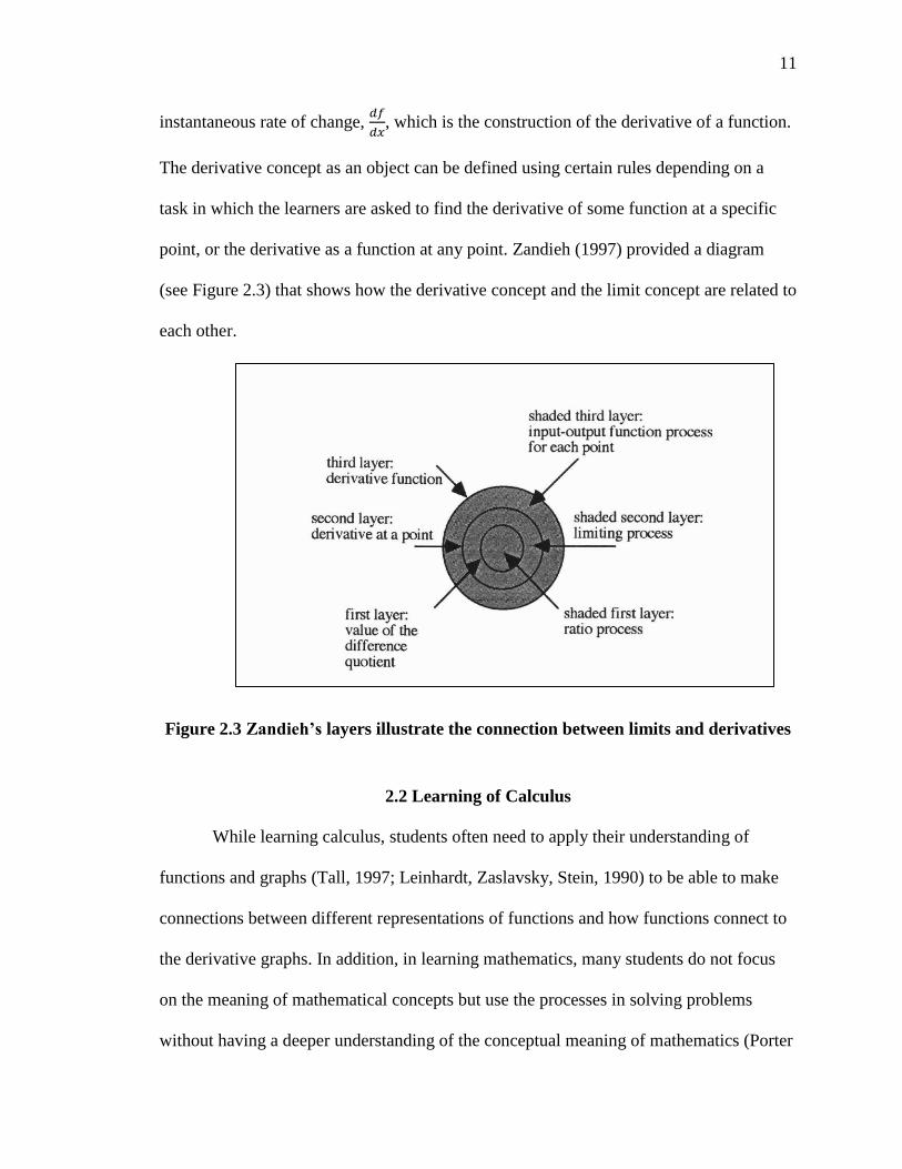
instantaneous rate of change, 𝑑𝑓

𝑑𝑥, which is the construction of the derivative of a function.

The derivative concept as an object can be defined using certain rules depending on a

task in which the learners are asked to find the derivative of some function at a specific

point, or the derivative as a function at any point. Zandieh (1997) provided a diagram

(see Figure 2.3) that shows how the derivative concept and the limit concept are related to

each other.

Figure 2.3 Zandieh’s layers illustrate the connection between limits and derivatives

2.2 Learning of Calculus

While learning calculus, students often need to apply their understanding of

functions and graphs (Tall, 1997; Leinhardt, Zaslavsky, Stein, 1990) to be able to make

connections between different representations of functions and how functions connect to

the derivative graphs. In addition, in learning mathematics, many students do not focus

on the meaning of mathematical concepts but use the processes in solving problems

without having a deeper understanding of the conceptual meaning of mathematics (Porter

12

& Masingila, 2000). Calculus concepts were learned where students implemented the

exact processes of solving problems, yet lack the understanding of the underlying specific

concepts. When calculus students have learned of the concepts of the subject, they can

extend and emphasize their knowledge when memorizing formulas. In this section, I will

discuss the connections between calculus, functions and graphs, how students learned the

calculus concepts, and difficulties students encountered.

2.2.1 Calculus in Its Connections with Functions

Functions are a necessary concept in learning mathematics, calculus in particular,

and is a foundational concept in teaching and learning mathematics. Students must

understand functions to succeed in the subsequent mathematics classes. Burns (2014)

states: “It is of vital importance that students learn and come to a clear understanding of

functions in order to succeed in mathematics courses” (p. 8). Researchers in the

mathematics education community have done many studies on teaching and learning

functions. Functions were beginning their notion in terms of describing the variables x

and y. Then, Tall (1997) discussed in the twentieth century, the “set-theoretic definition”

of function had been defined from a “visual idea of graph” (p. 9). Functions are difficult

concepts for students and often cause conceptual difficulties. Researchers in mathematics

education have studied function concepts and their relationships with calculus concepts.

They have investigated how they are taught and learned (e.g., Tall, 1997; Leinhardt,

Zaslavsky, Stein, 1990; Park, 2015; Orhun, 2012). They found that students’ difficulties

appeared when students made connections between functions and graphs, for example,

finding the equation of a function given with graph. Also, the misconceptions of

functions found in students’ grasping concepts of variables that are not actually shown on

13

a graph. They were not able to use the mathematical language of the graphs to describe

the functions.

A recent study of students’ misconceptions on functions and their derivatives by

Burns (2014), focused on investigating students’ insights and “students’ understanding of

the vertex of the quadratic function in connection to the concept of the derivative by use

of the think-aloud method…” (p.9). He found that most of the students had lacked an

understanding of the vertex of a quadratic function, and students did not fully understand

how the vertex of a quadratic function shaped to the derivative concepts. Misconceptions

were also found when the students applied the derivative in application problems. He

suggested that educators should apply more effort to emphasizing the concept of

functions, and that students need to understand these concepts fully before they learn

about derivatives in calculus. He also stated students need to develop their understanding

of the two concepts: the quadratic function and its derivative. Then, they would be able to

think about the derivative of a quadratic function in terms of the graph as the slope of the

tangent line, as instantaneous rate of change, or as velocity (Burns, 2014). According to

Burns, “this emphasizes the importance of understanding quadratic functions and

functions in general as a pre-requisite to understanding calculus” (p. 110).

2.2.2 Calculus and Its Representations with Graphing

Researchers have analyzed students’ understandings of the derivative concept

with graphing manipulations, such as the ‘action-process-object-schema’, or APOS,

theoretical framework used by Asiala, Cottrill, Dubinsky, & Schwingendorf, (1997).

Also, studies in mathematics show that using graphing skills is a possible technique to a

better understanding of calculus in general (Orhun, 2012; Tall, 1997; Leinhardt,

14

Zaslavsky, Stein, 1990). For example, when students experience multiple representations

while learning derivative concepts they made the connections between algebraic

expressions and their graphs of functions (Gravemeijer & Doorman, 1999; Tall, 1997;

Park, 2016; Tall & Vinner, 1981; Orhun, 2012; Kendal & Stacey, 2003). Tall (1997)

claimed that a graphing calculator is an alternative tool to help students understand

functions and their derivatives better. For instance, when students learn the derivative of

functions using visual representation such as graphs (e.g., from Rogawski’s & Adams

(2015) calculus textbook), they can make visual connections between the original

function and its derivative, such as the slope of the tangent line or the secant line on the

curve (see Figure 2.4).

Figure 2.4 Graph of a function and its derivative.

15

Recently, Park (2015) emphasized the derivative as a function on a graph. She concluded

the following:

In discussing the derivative as a function on the graph, the instructors quantified

the derivative as a number mainly by using functions with limited graphical

features such as linear functions or functions with horizontal tangents, they

quantified the derivative as “positive” or “negative” on an interval rather than as

numbers showing how the derivative changes as x changes (p. 246).

2.2.3 How Students Learn Calculus

Researchers have been investigating and exploring students’ learning of

mathematics in general and calculus courses in particular. They have suggested a variety

of ways to explore how students learn calculus. For instance, Tall & Vinner (1981)

discussed students’ understanding of calculus in terms of concept images and concept

definitions. On one hand, they stated that the concept definition is composed of “words

used to specify that concept,” whereas the concept image is holding a certain concept of

“all the mental pictures and associated properties and processes” (p. 2). Students can

develop their mathematical understandings through a variety of representations when

they apply them to solving problems. Furthermore, these representations might help

students make connections between memorizing rules and understanding the conceptual

meanings of Calculus I (Park, 2015; Tall & Vinner, 1981; Tall, 1997). Some students see

the value of using technology such as a graphic calculator while other students may not

use graphic calculators effectively. Nevertheless, some prefer to use one type of symbolic

representation to learn; whereas, others prefer to use multiple-types of representations in

learning concepts (Tall, 1997).

Also, calculus can be learned by creating a deeper understanding of the

conceptual meaning of mathematical concepts such as functions, limit, velocity, and

16

distance and by developing skills to apply these concepts. Asiala, Cottrill, Dubinsky, &

Schwingendorf (1997) have studied students’ understandings of a function and its

derivative. The authors in this study described the ‘instructional treatment’ that they

designed to learn about and compare the performance of students receiving the

researchers’ instructional methods, versus students receiving methods traditionally taught

in calculus courses. They explored the effectiveness of the instructional approaches on

the students’ outcome in learning functions and derivatives. Also, the researchers

investigated the instructional approaches of teaching calculus concepts and discussed the

conceptual/procedural understandings of the calculus courses by examining the effects of

writing tasks in order to learn mathematics (Porter & Masingila, 2001; Habre & Abboud,

2006).

Porter & Masingila (2001) investigated students’ conceptual understanding and

how they used the mathematical procedures in learning calculus by examining two

different groups of students, the WTLM group “Write To Learn Mathematics” and a

“non-writing” group. Porter and Masingila’s study focused on written tasks where

students engaged to discuss their thinking. The written tasks were used to test students’

insights and thinking about calculus. The study showed that there were no significant

differences between the two groups; no evidence showing different effects on the WTLM

activities rather than the non-writing activities. However, students from both groups were

able to communicate their understanding of the concept. In another study conducted by

Habre and Abboud (2006), they explored on how students learn function and its

derivative by two different approaches, a traditional Calculus I course and a reformed

Calculus 1 course, which had more effort on visualization. The aim was to investigate

17

students’ understanding of a function and its derivative geometrically and analytically

using the two curricula. Authors conducted interviews with students during the period of

their experimental course and they found that most of the students had complete

geometric understanding on the derivative concept, but they failed when they were asked

to define the derivative.

In the field of mathematics education research, researchers need to pay attention

to the intellectual processes required rather than an emphasis on the mathematics to be

taught. Some researchers focus on the students’ experiences of applying concepts such as

velocity, distance, and acceleration (Tall, 1997). Furthermore, these concepts can be

reproduced with computer simulations, as Tall (1997) stated that driving a car can be

“linked to numeric and graphic displays of distance and velocity against time” (p. 3).

Applying this process of learning will open the window to available representations of

teaching and learning calculus according to Tall (1997):

This widens the representations available in the calculus to include:

enactive representations with human actions giving a sense of change,

speed, and acceleration,

numeric and symbolic representations that can be manipulated by hand or

by computer, including the possibility of programming by the student,

visual representations that can be produced roughly by hand or more

accurately and dynamically on computers, and formal representations in

analysis that depend on formal definitions and proof (p. 3).

These representations (e.g., symbolic, numeric, etc.) and other manipulations are useful

tools for calculus students to enhance their learning of calculus concepts. Learning

calculus has been developed from very traditional ways of solving problems symbolically

to more sophisticated procedural ways of thinking and visualizing (Tall, 1997).

18

2.2.4 Challenges and Promises

One of the challenges in learning calculus for students is when teachers are using

new approaches to teach the courses, making changes in calculus curriculums, adopting

unpopular practices, and/or using technology (Habre & Abboud, 2006). In fact, while

students often do well on routine problems that are familiar to them and had practiced

before in class, researchers have reported that students often struggle when they are faced

with non-routine problems in calculus courses (Selden et al., 1994) (as cited in Habre &

Abboud, 2006). For example, experts provided an unusual test for calculus students

asking them to write down as many of their ideas as possible. These problems on the test

were chosen to examine students’ understanding of the function and its derivative, how

this could impact their answers as they had in their mind patterns of skills and procedures

to solve problems.

However, challenges may also occur in learning calculus when a student learns

the concept of calculus negatively or without having a deeper understanding of what they

have learned in the class. For instance, college students usually have misunderstandings

of the prerequisite concepts of calculus, such as functions, which is due to their

background knowledge. In a study reporting on students’ understandings of the chain

rule, for example, the authors found a large number of students had difficulties in dealing

with decomposition and composition functions (Clark et al., 1997). In addition,

researchers have identified some calculus students’ misconceptions about the rate of

change concepts as related to the idea of relations between concepts such as “average rate

of change,” “average value of a continuous function,” and “arithmetic mean”

(Bezuidenhout, 1998).

19

2.3 Teaching of Calculus

Calculus is always a challenging area for college students and it is a requirement

for many majors. It is a complex course with many connections in mathematics.

Therefore, in this section, I will discuss the instructional methods and curricula materials

for teaching calculus as well as the use of technology.

2.3.1 Curricula Materials

Contextual materials in teaching calculus play a significant role in students’

understandings of calculus concepts. For instance, in the past, Clark et al. (1997) studied

two different groups of students; one taught traditionally, called, “lecture-recitation

course”, which focused on students constructing the concepts of calculus from lectures,

class group work, and assignments. The study showed that students from the traditional

classes were not engaged in using computers or programs. The second group taught with

a method known as ‘𝐶4𝐿’ “Caculus, Concepts, Computers, and Cooperative Learning”,

which is used to help construct understanding and applying of the Chain Rule. Authors in

this study explored students’ understanding of the chain rule by conducting interviews

with students from both groups. As a result, they interpreted findings on understanding

the chain rule involved the “building of a schema” (p. 31) through three stages called

“Intra, Inter, and Trans”. Among these three stages: the Intra focused on a single object

from other actions, processes, or objects, the Inter focused on recognizing relationships

between different schemas, and finally the Trans focused on constructing the

relationships discovered in the Inter stage. As result, they found many students did well

using the algebraic way and they could realize rules and procedures for example,

recognizing the power rule and providing general statement of the chain rule but “had not

20

yet constructed the underlying structure of the relationships” (p. 10). They also found that

students from traditional classes did poorly in solving tasks than students from the other

group. Also, a national survey conducted by the MAA (Mathematical Association of

America) reported on instructor pedagogy and its impacts on students’ attitudes in

calculus college courses (Bressoud, Carlson, Mesa, & Rasmussen, 2013). The survey

reported on many different selected institutions conducted with STEM majors. According

to the survey, the context of Calculus I provided in 17 selected institutions was offered

and formatted based on the institutions’ goals and needs. Usually the Calculus I at college

level in the United States covers basic concepts of differentiation and integral calculus,

but the course contents in Calculus I have changed over time (Burn & Mesa, 2013). The

classrooms’ size in many of the universities is about 30-40 students, and in some of them

the use of technology such as CAS, online work, and graphing calculator were

incorporated. Also, according to the survey, students in Calculus I classes engaged in

practicing projects, presentations, and group works. Instructors who are teaching

Calculus I among all the institutions range in background between PhD, Master, and

Graduate Teaching Assistant (Selinski & Milbourne, 2013). More recently, Park (2015)

reported how instructors taught the derivative as point-specific and as a function from her

study. Park (2016) also analyzed calculus textbooks and their effectiveness on

instructors’ teaching practices and students’ learning in specific topics in calculus such as

with derivatives. Those studies demonstrated how instructional approaches of using

curricula materials influence the students’ outcome and their understanding of the

calculus concepts.

21

2.3.2 Classroom Instructional Methods

Besides the importance of the curricula materials, instructors need to be careful

when they apply their mathematical knowledge and to create efficient approaches that are

relevant to their classroom. Therefore, the instructional approach is important because it

is the key, for the instructors and students, to communicate their ideas in the classroom.

Tall, Smith, and Piez (2008) argued that the subject of calculus serves not only to

solve mathematics problems or mathematics applications, “but also [calculus serves] as a

natural pinnacle of the beauty and power of mathematics for the vast majority of calculus

students who take it as their final mathematics course” (p.2). They suggested how

calculus should be taught based on the results of their study at that time. Calculus

traditionally introduces the concepts of differentiation and integration in terms of

symbolic manipulations and applies these concepts to solve problems. Tall (1997)

indicated that there are different instructional methods used to teach calculus, and some

methods are more appropriate for elementary versus advanced mathematics education.

Furthermore, it is clear that students’ backgrounds and knowledge of calculus are the

biggest challenges that may inform instructors when determining their instructional

practices.

In the past, researchers categorized different representations to teach and learn

calculus and found that there were three ways to present calculus’ knowledge (e.g.

functions). First is the numerical way for solving problems as functions, such as (𝑦 =

3𝑥2 + 𝑥 − 5). Second is the graphical way, which works for investigating the shape of

functions (visual image of graphs of a function “𝑓(𝑥)”). The third is the symbolic way,

22

which is appropriate for the use of Computer Algebra Systems (CAS). These

representations can be used independently or together (Ferrara, Pratt, & Robutti, 2006).

Hardy (2009) showed that, at her college, the calculus course material was created

collectively by committees who were responsible for designing and structuring the

course. At the time of her study, the college, where she had conducted her study, had

nineteen sections of the course and 14 instructors. The committees selected a beneficial

textbook, practices, homework, tasks, and a final exam. Although the instructional

methods varied among instructors, every student in each section learned the same topics

and practiced the same information on the homework and for their test. Students in one

section and in another section compared their notes and studied together in groups. This

treatment of instructional materials, which were limited and given by the college, was

also investigated. The study found that students depended on a set of steps and

instructions when they solved problems, which caused a lack of understanding of the

concept, and led students to fail when they apply to a non-routine problem. The routines

tasks had a negative impact on the students when they generalized their understanding

with practicing by norms instead of practicing by rules. According to Hardy (2009),

“students' models are emphasized and validated by the tasks proposed by the institution”

(p. 21).

Researchers have found and adopted a framework for creating instructors’

teaching practices in teaching derivative concepts. For example, Asiala, Cottrill,

Dubinsky, & Schwingendorf (1997) had addressed three elements of those constructions:

“theoretical analysis, instructional treatments, and observations and assessments” (p. 2).

The theoretical analysis had a place to suggest a “genetic decomposition” that the learner

23

has a mental construction (such as the ‘APOS theory’) to develop his or her

understanding of the concepts. The instructional methods used depend on the basis of

“genetic decomposition of mathematical concepts”. Moreover, this instructional method

that helps students make connections between calculus concepts is called “the ACE

teaching cycle (Activities, Class tasks, and Exercises)” (p. 2). As a result, from their

study, authors found that students could use mathematical programs, engage in group

work to discuss their results in problem-solving, and “investigate mathematical concepts

using a symbolic computer system” (p. 2) while they were learning derivatives.

Even though there are a small number of studies about teaching derivatives in

calculus courses, there is a study from Bezuidenhout (1998) who suggested that calculus

teachers must consider students’ fundamental misconceptions concerning main concepts

in first-year calculus such as “the rate of change” and other fundamental concepts of

calculus;

An important challenge to mathematics educators is to create innovative curricula

and pedagogical approaches that will provide calculus students with the

opportunity to construct relevant and powerful concept images and allow them to

reflect on the efficacy and consistency of their mathematical thinking (p. 397).

Researchers have noted that calculus is a difficult subject, and they have tried to

study and explore efficient instructional strategies to help students acquire the

foundational knowledge of calculus concepts.

2.3.3 Technology in the Classroom

Using technology in college calculus courses is one didactic way to learn and

teach calculus and it has been become more prevalent as its availability has increased.

The use of technology, such as CAS, was discovered in calculus classes from the past, for

example, Kendal & Stacey (2000) discussed how students acquire conceptual

24

understanding of differentiation incorporating graphical, numerical, and symbolic using

computer algebra systems (CAS) in the classrooms. Researchers have responded to many

questions and issues on the teaching of variables and expressions with technology. Below

is an example from one group of those researchers (Ferrara, Pratt, & Robutti, 2006):

Trends in emphasizing students’ learning and multiple views of concepts through

multiple representations clearly appear, but so little, if not any, attention has been

paid to curricular aspects and teachers’ knowledge or teaching practice up to now

(p. 246).

Nonetheless, much technology has evolved to be used in calculus classrooms, such as

CAS, Mathematica, Maple, and Derive (Tall, Smith, and Piez, 2008). Experts have tried

to explain the concept of calculus in a variety of ways, from the traditional methods and

algorithm structures to using graphing software (Tall, Smith, and Piez, 2008; Ferrara,

Pratt, & Robutti, 2006; and Habre & Abboud, 2006). To develop students’

understandings, Haber and Abboud (2006) examined an experimental calculus course,

and focused on the use of “Autograph”, calculus software, and a calculator to help

students comprehend the concepts of a function and its derivative. The results showed

that a large number of students failed to find the derivative geometrically and used the

mechanical methods, as a result of the fact that the “mathematical definitions are

traditionally analytical, creating an obstacle in the minds of the students” (p. 68). They

also concluded that the new approach of the technological approaches such as using the

software Autograph was challenging for many students and benefitted few students.

Using technology such as graphing calculators and online homework helped

students to understand and grasp the concepts easily because it helped combine both the

numerical and graphical approaches (Zandieh, 1997; Leinhardt, Zaslavsky, Stein, 1990;

Kendal & Stacey, 2000). Technology, such as the use of a graphing calculator, allowed

25

entering texts or numbers, drawing a graph, and working while studying calculus

concepts (Kendal & Stacey, 2000). For example, the use of graphing calculators could

help students to visualize the relationship between the rate of change (tangent), or the

slope of the tangent line, and the derivatives, thus, enhancing their understanding of the

concepts rather than just relying on the algorithm and calculations by hand. When

teachers use symbolic representations to find the derivative of a given function without

providing graphical representations (i.e., drawing by hand, or using GeoGebra, graphical

calculator, etc.), students may solve the problem using arithmetic without having a deeper

understanding of the relationship between the value of the derivative and the slope at a

specific point. The use of technology may help students to understand the concepts by

visualizing them. Individualized learning could be developed when students learn and

apply their mathematics concepts by using some helpful devices such as a graphing

calculator. Researches have argued the impact of incorporating technology in calculus

classrooms, for example Bressoud, Carlson, Mesa, & Rasmussen (2013) from the MAA

National Study of College Calculus reported three different factors of pedagogical

characteristics: “good teaching”, “technology”, and “ambitious teaching”; and have found

the use of “technology” was not significant; whereas, “ambitious teaching” had a

negative effect and “good teaching” had a positive effect on students. In the survey, they

reported that most of the instructors use graphing calculators and online homework

grading systems. They found an increasing use of graphing calculator in the classrooms

and greater percentage of instructors’ permitting graphing calculator use on exams.

When technology such as ‘WebAssign’ arrived in calculus, it allowed new

methods and provided a new learning environment to develop in the mathematics

26

classroom and in calculus demonstrated tasks might be solved using graphing calculators

(Tall, 1997). There are many advantages of using the technological way of teaching and

learning calculus. For example, it is convenient that students can use them anytime and

anywhere as needed. This technological way would encourage creativity and possible

new strategies in the teaching of calculus. It is very important to increase emphasis on

how to make calculus a more understandable subject for various students by helping

students learn a variety of helpful ways (e.g., increase of visualizing graphs of functions

and their derivatives) to comprehend calculus through the use of technology.

2.4 Mathematics Classroom Discourse

In every classroom, language is a powerful tool for social interaction and it is also

a way to deliver concepts to the learners. Language in mathematics plays a critical role in

establishing the learning environment in the classroom (Walshaw & Anthony, 2008;

Moschkovich, 2010). The use of appropriate language in the mathematics classroom

helps instructors to improve the learning and teaching of mathematical concepts, and

researchers have reviewed the relationship between language and mathematics learning,

asserting their complexity in classroom environment (e. g., Moschkovich, 2010). It is

often seen that in mathematics and calculus classes, teachers usually do not give attention

to the language used to deliver their ideas and concepts of mathematics (Schleppegrell,

2010). For example, when instructors discuss any of the mathematical terms incompletely

defined and shift the students’ attention toward the procedure rules instead forcing

thinking and reasoning, students’ struggles will show up and meet a lack of establishing

information foundation. Walshaw & Anthony (2008) noted that the use of language in the

mathematics classroom supports the students to be more engaged in mathematical

27

discussions and helps the teachers to understand their students better. According to them,

“Reframing student talk in mathematically acceptable language provides teachers with

the opportunity to enhance connections between language and conceptual understanding”

(p. 530). This creates an overall learning and contributory environment to engagement

from both educators and learners.

Mathematics is a difficult subject as compared to other subjects. Language itself

is very important in mathematics. Sometimes, students use incorrect mathematics

terminology, which leads to negative impact on students’ learning and makes a gap in

their future learning (Gutiérrez, Sengupta-Irving, & Dieckmann, 2010; Schleppegrell,

2010). There are a number of words that have a specific mathematical meaning such as

“to cancel”, or “to eliminate”, but these have totally different meanings in daily life

conversation. For example, in our daily life, we use ‘cancel’ when we cancel a meeting,

but, in mathematics classroom, the word ‘cancel’ usually means to ‘simplify’

expressions. Discourse practice in the classrooms could shed light on how mathematical

words are used. Instructors communicate the mathematical concept with vocabulary and

students must learn that vocabulary to build a greater understanding of the mathematical

meaning. Students must be able to think and reason mathematically when they learn

mathematical ideas. Mathematicians aimed to investigate teacher practices and tried to

make changes in their instructional approaches when they taught mathematics in

secondary school. For example, (Ball, 1993) focused her study on the development of

teaching practices when she was teaching mathematics at elementary level (8 – 9 years of

age). According to her, “Students must learn mathematical language and ideas that are

currently accepted. They must develop a sense of mathematical questions and activity”

28

(p. 376). “In the context of teacher development” Schleppegrell, (2010) declared that, “a

focus on language can help address the difference between questions like do you know

mathematics? and can you talk about mathematics?” (p. 105). Allowing instructors to

communicate their ideas with students makes their students become involved in

discussions and talk about their mathematical knowledge. Therefore, it is important to

take account of instructors’ approaches and the ways they teach and communicate the

Calculus I course.

2.4.1 The Rule of Questioning in Classroom Discourse

In classroom discourse practices, questioning plays an important role in

understanding different concepts (Walshaw & Anthony, 2008) because it is the design of

communications that math instructors must create in the classroom. Questioning is a way

to guide instructors in useful discussions where students can engage in the mathematical

discourse. The quality of interaction with students and the use of discursive approaches in

classrooms has a special impact on the learning process. According to Walshaw and

Anthony (2008), there are two critical techniques in the productive environment of

mathematics classroom discourse. The main object of these techniques is to involve the

students in active questioning by the use of conversations between students and teacher.

These conversations include sharing of ideas and receiving feedback from instructors and

other students. This helps improve student understandings of the mathematical

knowledge. In another study conducted by Cazden & Beck (2003) “handbook of

discourse process”, the authors made an emphasis on the ways instructors ask questions

that help in keeping classroom discussions with students moving forward and make

students think and reason about the mathematical knowledge, and asking them to explain

29

their answers and reasoning with their peers. According to Cazden & Beck (2003),

“Instead of the traditional pattern of classroom talk in which teachers ask test-like

questions and students give short, test-like answers, teachers are being asked to lead

discussions that stimulate and support higher order thinking” (p. 165). In their study of

classroom discourse, they also reported on how researchers and instructors believed the

teacher’s questions could have powerful effects on students’ learning.

Questioning in classroom discourse helps instructors understand their students

and then inform their instructional approaches by determining what questions they should

ask depending on students’ knowledge. The decisions that instructors make when they

plan their lessons include questions that help the students engage in the mathematical

discourse, exploring and reasoning. Discourse in classrooms also allows instructors to

think not only about their students’ understanding, but also about the approaches they use

in their everyday practices, and how well they understand the mathematical ideas and

present them in productive ways. According to Walshaw & Anthony (2008), they argued

about how the students’ outcome is influenced by teaching:

In this conceptualization, teaching is influenced by adaptive rather than additive

factors and by interactive rather than isolated variables. This means that the

outcomes of teaching are contingent on a network of interrelated factors,

conditions, and environments. These are the factors and conditions that shape

how, and with what effect, mathematics is taught and learned (p. 542).

2.4.2. Discourse in the Calculus Classroom

Gaining effective mathematical communication in the classroom is complex when

it is not clear to students and without explicit teaching. In the mathematical classroom,

the discussions related to mathematical concepts are critical in developing proficiency in

learning and teaching of mathematics (Ball, 1993). Discourse in the classrooms consists

30

of textbook definitions and approaches that mathematics instructors use to communicate

their mathematical ideas. In the mathematics classroom, there is a close relationship

between allowing the students to talk about math and their understandings of

mathematics. In an effective learning environment, the teacher must be flexible and

careful to encourage a safe and equitable space for classroom discourse. Discourse in

mathematics and calculus classes is the way that describes student-instructor interactions,

language, vocabulary, and communications skills. Nardi, Ryve, Stadler & Viirman (2014)

stated that “In this sense, learning mathematics, or any other topic, is an initiation into a

discourse, where discourse is meant as a type of communication that characterizes a

particular community” (p. 184). Considering and examining mathematics through the

discourse approach is a new line of inquiry in the area of mathematics education research,

and studies that investigate teaching and learning of the calculus in the context of

classroom discourses are very rare.

In existing studies, researchers (e.g., Park, 2015; and Nardi, Ryve, Stadler &

Viirman, 2014) explored the mathematics discourses in the teaching and learning of

calculus. For example, in the study of the derivative as point-specific and as a function

conducted by Park (2015), the researcher examined three college instructors in how they

addressed the concept of the derivatives with word uses and visual mediators. Her study

also found how instructors could make connections between visual mediators when

introducing the derivative concepts with algebraic notations, graphing illustrations, and

symbols. A study conducted by Nardi, Ryve, Stadler & Viirman (2014) showed students’

interactions and thinking about the concept of function through the communication

approach. Results from their study found to expand the communication approach by

31

developing Sfard’s commognitive approch in analyzing the learning and teaching of

mathematics.

According to Sfard (2008), discourse is defined in terms of mathematical

thinking as “the commognitive vision of mathematics as a type of discourse – as a well-

defined form of communication, made distinct by its vocabulary, visual mediators,

routines and the narratives it produces” (p. 433). In the following chapter, I will provide

an explanation for Sfard’s commognitive framework with four features of the

mathematical discourse: word use, visual mediator, routines, and narrative.

32

CHAPTER THREE: THEORETICAL FRAMEWORK

In this section, I discuss mathematical discourse through Sfard’s framework, the

commognitive approach, in the context of calculus, and I adopted this framework in

analyzing my data because it helps me to guide and discuss the instructional approaches

and the way instructors teach Calculus I course. Also, Sfard’s framework contains useful

tools for research designs and discussions; it allows me to observe classes and to take a

deeper look into why and how instructors teach calculus in the United States. First, Sfard

characterized mathematics discourse by four components: word use, visual mediators,

routines, and endorsed narratives. Second, I describe in detail how to analyze the

discourse with regards to the derivative/ limit concepts using primarily word use and

visual mediators.

3.1 Word Use

Word use is an important key to teaching and learning in calculus courses.

Mathematics discourse about calculus is a discourse in which we use a lot technical terms

in the text of calculus. For example, in calculus discourse, we use words such as

functions, limits, derivatives and integrals that would be addressed in any level of

calculus classroom. In this study, the instructors’ words used in teaching limit and

derivative concepts (and any related concepts such as Rate of Change (RC),

Instantaneous Rate of Change (IRC), slope, slope of tangent lines, secant lines) are

observed and their use of those words are investigated. The way instructors’ use words to

explain what they mean by limit or derivative are important because students need the

33

opportunities to express themselves and make coherent sense of the relationship between

the concepts of calculus. For example, there is a connection between the concepts of the

average rate of change, the definition of limits as “approaches” and computing the

derivative. The more clearly the instructor’s word use illustrates derivative connections

with functions and derivative connections with limit concepts, the more students are able

to grasp and articulate calculus concepts precisely.

3.2 Visual Mediators

Visual mediators are operationalized as objects that are considered as the

instructors’ way of addressing the derivative concepts or limit concepts in calculus

classrooms. In calculus discourse, visual mediators are often represented as graphs,

diagrams, tables, symbolic notations such as [𝑓′(𝑥) 𝑜𝑟 𝑑

𝑑𝑥], algebraic expressions,

numerical values, and equations that serve as tools for communication. For instance,

visual representations which instructors used to find the derivatives from given functions

or drawings of functions and their derivatives are considered as visual mediators. In this

study, in the Calculus I classroom, the visual mediator is described as graphs of functions

and their derivatives, notations, expressions, and numerical values of calculating the limit

or the derivative of functions using differentiation rules. Visualizing graphs allows

students to think about their understanding of the derivative concepts and encourages

them to use multiple approaches to connect their understanding with symbolic

representations while applying the process.

3.3 Routines

In a calculus class, routines are defined as the repetitive patterns in instructors’

communicating derivative concepts. Routines can be described as what kind of tasks

34

instructors are offering when they respond to the concepts underlying the derivative, or

what the usual actions of computing the derivative are. It could also be the descriptive

techniques of calculating the concept of derivative (e.g., average rate of change,

instantaneous average rate, slope, etc.). In addition to the calculus classroom, routines are

embedded in descriptive teaching practices that illustrate the derivative concepts (e.g., by

the limit definition, slopes, graphing, finding the area, anti-derivative) while the

instructors are introducing them in their classrooms. For example, while finding the

derivative of a function by computation, an instructor might use a graph to illustrate the

slope of tangent lines and to help connect the function and its derivative with the original

one. Another instructor might use only the algebraic expressions or the symbolic notation

of the definition to find the derivative without sketching graphs. Also, in calculus classes,

routines could be found on the process of how instructors define velocity, rate of change,

and slope at a point.

3.4 Endorsed Narratives

In mathematical discourse, the endorsed narratives are the statements of the

mathematical concepts as definitions, theorems, or identified justification. For example,

in calculus, instructors may endorse a narrative about the derivative of a constant as zero

by comparing the slope of the tangent line in a graph of a constant function (e.g., 𝑓(𝑥) =

𝑎) with horizontal line and showing that visually with a graphical interpretation.

Using Sfard’s discursive framework, my study is designed to investigate 1)

college instructors’ interactions with students in calculus classrooms, 2) the way college

instructors communicate the concept of derivatives connecting the multiple

representations of addressing the concepts from discourse perspective, 3) calculus

35

instructors’ instructional approach in terms of their use of technology and contextual

materials, while communicating derivatives and differentiation. In this study, I focused

my analysis primarily on the area of word use to have a better understanding of how

instructors communicate the concepts of derivative and limit with their students in

college classrooms. I will also include visual mediators in my analyses as they were used

in different illustrations such as symbols, graphs, and expressions.

36

CHAPTER FOUR: METHODOLOGY

All classroom observations were completed in the spring of 2016 at a

northwestern university in the United States. The classroom observation data and

interview data were collected and analyzed.

4.1 Setting

The classroom observations were conducted in Calculus I classes. This course

was chosen because it offers knowledge and concepts that are related to differentiations

and derivatives, such as the slope of the tangent line, and the limit of the average rate of

change, etc. The calculus textbook (Rogawski and Adams, 2015) that the instructors used

includes seventeen chapters with a variety of topics such as Functions and Models

(Chapter 1), Limits and Derivatives (Chapter 2), Differentiation Rules (Chapter 3),

Application of Differentiation (Chapter 4), Integrals, etc. (Stewart, 2015). Derivatives

and differentiation are generally introduced early in the semester because they appear

early in the textbook. The mathematics department of the university offers seven sections

of Calculus I each semester. The classroom observations focus on Chapter 2 (Limits and

Derivatives), Chapter 3 (Differentiation Rules), and Chapter 4 (Applications of

Differentiation). Calculus I instructors usually spend two to three weeks covering those

topics, which is around six to seven class meetings (I obtained this information in my

personal communications with instructors during the pilot study). The class size of each

Calculus I class was about 30-40 students.

37

4.2 Participants

The participants in the study were mathematics instructors who teach Calculus I at

the university. Usually, these mathematics instructors have received their Master’s

degrees or Ph.D. in mathematics. In this study, I recruited three instructors, Henry, Dina,

and Jack, and their participation in the study was completely voluntary. To learn more

about their instructional approaches and ways they communicate with their students in

calculus, I conducted a 15-20 minute one-on-one informal interview with each of them

after their first or second classroom observations.

4.3 Data Collection

The data sources included field notes, recordings from interviews with instructors,

and classroom recordings (video recordings with students’ permission). I conducted a 15-

20 minute informal interview with each instructor to get some information about their

educational background, the challenges of teaching and learning derivatives and

differentiations, the instructional approaches they use to teach these topics, and their

plans to include technology such as computers and graphing calculators. All interviews

are recorded and transcribed. I have six class observations from each instructor across

two to three weeks to investigate their instructional approaches and to observe their

interactions with students. All classroom video recordings are transcribed and coded. I

compiled all the data to identify themes and to analyze their mathematical discourse.

38

CHAPTER FIVE: FINDINGS

As described earlier in the literature review, the teaching and learning of calculus

primarily focuses on functions, limits, and derivatives. Therefore, my analyses in

observing calculus classrooms included analyzing instructors’ use of mathematical words

(word use) that relate to the concepts of limits and derivatives, as well as their

instructional approaches of introducing those concepts and the way instructors

communicate these concepts.

5.1 Case 1: Henry’s Calculus Class Observation

Henry was one of the three participating instructors in this study. In my interviews

with Henry, I learned that he has a Master’s degree in mathematics, and he has been

teaching the Calculus I course for three semesters, since spring of 2015. Henry is the

newest instructor among the three instructors in the study with teaching experience with

Calculus I. He is part of a collaborative group in which the mathematics department

supports and guides in teaching Calculus I. Instructors in this group meet regularly to

discuss their course material and they provide the same exam for all of their students.

They have a similar class setting, where the students are distributed in groups of 4-5

students. Generally, the instructors give 20-30 minute lectures and then the students are

mandated to work in groups or individually to complete online work on a required

website that is called “WebAssign”.

I observed his Calculus I classes (n = 6) during the spring of 2016 on Mondays

and Wednesdays. Each lesson is labeled as “L” with the lesson number 1, 2...6. Each

39

class observation took place for about 105 minutes (one hour and 45 minutes). The class

size consisted of about 30 students. The students in this classroom were sitting in nine to

eleven groups of 2 -5 students. Each student had his/ her laptop because he or she had to

work on his or her online homework at the end of each class time. Henry usually lectured

for about 40 minutes and the remainder of the class time was spent doing the online

homework on “WebAssign”. My analyses, in this case, will focus on how the instructor

introduced the concepts of limits and derivatives and the way he communicated his

thinking to his students during the 30-40 minutes of discourse instruction.

5.1.1 Word Use

First, in this section, I will show a list of quotes from Henry’s classroom

observations. These quotes were chosen to highlight the word use when he discussed the

concept of limit and derivative, and to recognize how he used the same words such as

“slope” or “rate of change” in the contexts of the derivative and limit. The quotes are

verbal narratives from the classroom observations while he was discussing the concepts

of derivatives and limits.

Henry’s verbal narratives about the limit concept

“What does the section say here [he is gesturing on the board] how do we read

that? The derivative, yeah the derivative of h at t equal 2. Yeah, t equals two.

Let’s write it in terms of stuff here. We know the limit of [he is writing on the

board] we know the limit in the average rate of change is what? as u approaches

2? How would we shrink that interval [he is gesturing to the board] we’d like to

actually to calculate the instantaneous rate of change in 2 rather than the average

rate of change in the interval? We need to shrink the interval, right? That kind of

procedures we’ve been doing” [observation L1].

“What makes this interval skinnier; you just let u get closer and closer to 2 [S1].

Yeah! And that’s how we write that…we write what happens to our average slope

formula as u approaches 2. In other words, what is the limit of that calculation,

secant slopes as u approaches 2” [observation L1].

40

“… That is our instantaneous rate of change or our velocity this space, right?

Let’s think about a distinct, yeah, that’s our instantaneous velocity at t equal 2.

So, this is an important part, right? [he is gesturing to the board] This is, this is

what we mean by derivative. This is by definition is true; let’s put this means [he

wrote ∆ℎ

∆𝑡]𝑡=2]” [observation L1].

“If you want to find the derivative or the instantaneous rate of change at generic t,

another notation, prime notation [𝑑ℎ

𝑑𝑡= ℎ′(𝑡)] means the same thing the derivative

of h at t. that’s gonna be the limit of our secant slope formula, which is [he is

writing] (50-16(u+t)) as u approaches t” [observation L1].

In analyzing word use, I include the analysis of how Henry used mathematical

words such as limit, derivative, rate of change, slope, velocity, as well as how he

communicated those concepts using symbols, expressions, graphs and other visual

mediators. In Henry’s case, I focus my analysis, first, on the word “limit” as it was used

to articulate the concept in two categories: limit as a process and limit as an object.

As noted earlier, limit as a process is defined as the mathematical calculations of

computing the average rate of change, instantaneous velocity, difference quotient, or

slope numerically or symbolically (Park, 2015). For example, when students were asked

to find the limit of a function h when t approaching to 2, given a function h in height

ℎ(𝑡) = 100𝑡 + 50𝑡 − 16𝑡2, they applied 2 to the function in order to calculate the limit

and found a particular value of function, h, at this point, when 𝑡 = 2. First, Henry

discussed what a student had written on the board calculating the average rate of change

Δℎ

Δ𝑡 on the interval [2, n] and then he evaluated the limit of that average rate of change at

t=2, as he was talking to the whole class:

...What does this section say here [he is gesturing on the board] how do we read

that? The derivative, yeah the derivative of h at t equal 2. Yeah, t equals two.

Let’s write it in terms of stuff here. We know the limit of [he is writing on the

board] we know the limit in the average rate of change is what? as u approaches

2? How would we shrink that interval [he is gesturing to the board] we’d like to

actually to calculate the instantaneous rate of change in 2 rather than the average

41

rate of change in the interval? We need to shrink the interval, right? That kinds of

procedures we’ve been doing what makes this interval skinnier; you just let u get

closer and closer to 2 [S1]. Yeah! And that’s how we write that, we write what

happens to our average slope formula as u approaches 2. In other words, what is

the limit of that calculation, secant slopes as u approaches 2 [observation L1].

In this case, Henry used the word “slope” explicitly with terms “secant slope”

when he discussed verbally the limit as a process. In the process of his calculating the

limit he mediated the limit by words such as “How would we shrink that interval” and

“what makes this interval skinnier,” or for by describing the location in the computation

as when he said “you just let u get closer and closer to 2.”

The limit as a process was also observed when Henry was graphing secant lines as

to what he did (as a process) to highlight the concept of limits. For instance, when Henry

discussed the slope of the secant line over the integral [2, n], he interpreted the average

rate of change on that interval in terms of a graph. Verbally, he said:

We were working to compute the what we are calling the average rate of change

delta t over delta h [he is writing on the board] the average rate of change on [2,

n] [he wrote it] Think what it is? In terms of lines maybe. In terms of graph, this

number corresponds to [he is gesturing on the board ∆ℎ

∆𝑡𝑜𝑛 [2, 𝑛]] number secant

lines, yah, response to the slope of the secant lines. That’s what we gonna come

up with the whole number of secant sloped. This interval [2,u] and by definition

we know that f of h minus f of 2 over u minus 2, so delta h over delta t. we simply

plugged in …… [observation L1].

Limit as A Process

From all of my observations in Henry’s classroom, the limit as a process was

addressed with calculations of numbers and communicated with key words such as rate

of change, average rate of change, instantaneous rate of change, instantaneous velocity,

and slope. The following is the analysis of where these words were used in Henry’s

classroom when he introduced limits as process.

42

Average Rate of Change/ Rate of Change. Mathematically, the average rate of

change is defined as ∆𝑦

∆𝑥=

𝑓(𝑥1)−𝑓(𝑥0)

𝑥1−𝑥0, (Adams & Rogawski, 2015), where ∆𝑦 is the

change in y and ∆𝑥 is the change in x. In this case, the limit as a process was

communicated using the words ‘rate of change’ or ‘average rate of change’ when

computing the limit of a given function by calculating the ratio of the average rate of

change, ∆𝑓

∆𝑥=

𝑓(𝑥1)−𝑓(𝑥0)

𝑥1−𝑥0 over the interval [𝑥𝑜 , 𝑥1]. For instance, when Henry

demonstrated the limit of the function ℎ(𝑡) = 100𝑡 + 50𝑡 − 16𝑡2 over the interval [2, 𝑢]

where 2 was the fixed point, he calculated the average rate of change and then he took the

limit of that calculation as u approached 2, lim𝑢→2

(Δℎ

Δ𝑡) = lim

𝑢→2(−16𝑢 + 18) = −16(2) + 18.

Another example of limit as a process was when Henry was calculating the limit for the

same function but over the interval [𝑡, 𝑢] where was t the fixed point, lim𝑢→𝑡

(50 −

16(𝑢 + 𝑡)) = 50 − 32𝑡. In a different case, Henry provided a proof of a differentiation

rule when introducing it. For example, he calculated the average rate of change as a

process, given a function 𝑓(𝑥) = 𝑥2over [𝑥, 𝑥 + ℎ], as x was the fixed point and h went

to zero, and the limit of the rate change calculation was, limℎ→0

(Δ𝑓

Δ𝑥) = lim

ℎ→0(2𝑥 + ℎ) = 2𝑥.

He then explained:

Let’s calculate the average rate of change of the function [𝑓(𝑥) = 𝑥2] umm, I’m

goanna pick like this [x, x+h] Ok! So, how we should shrink this interval, I guess

figure it out. x is fixed, what we should do with h? Yeah, we should get in closer

and closer to zero. Good. Let’s do that average rate calculation [observation L1].

Instantaneous Rate of Change/ Instantaneous Velocity. Henry also used phrases

such as ‘instantaneous rate of change’ or ‘instantaneous velocity’ when he was solving

the limit as a process in a problem that gave a height of an object by a function at a

43

generic time (t) and thinking about it as a distance. Henry was computing the limit by

using these phrases as noted words to describe the process of the limit computations.

Mathematically, the instantaneous rate of change is defined by the following rule,

𝑓′(𝑥0) = lim∆𝑥→0

∆𝑦

∆𝑥= lim

𝑥1→𝑥0

𝑓(𝑥1)−𝑓(𝑥0)

𝑥1−𝑥0 (Adams & Rogawski, 2015). Based on this

definition, Henry illustrated that when students had calculated the limit of the average

rate of change in the previous function, where (𝑡 = 2), they actually were calculating the

instantaneous rate of change or the velocity at a distance in 2. Thus, after the calculations,

it provided a value in terms of feet per second,

𝑑ℎ

𝑑𝑡|𝑡=2 ≈ lim

𝑢→2(

Δℎ

Δ𝑡) = lim

𝑢→2(−16𝑢 + 18) = −16(2) + 18 = −14

𝑓𝑡𝑆𝑒𝑐⁄ .

Slopes. The limit as a process was also communicated with the word ‘slopes’

when calculating the basic algebraic calculation of the average slope formula, 𝑓(𝑥1)−𝑓(𝑥0)

𝑥1−𝑥0,

the slope of the secant line through the points (𝑥0, 𝑓(𝑥0)) and (𝑥1, 𝑓(𝑥1)). For example,

when Henry addressed the limit of the function ℎ(𝑡) = 100𝑡 + 50𝑡 − 16𝑡2 at 𝑡 = 2, he

was calculating the slope of the secant line on h as u approaches 2, Δℎ

Δ𝑡𝑜𝑛 [2, 𝑢] =

ℎ(𝑢)−ℎ(2)

𝑢−2=

100+50𝑢−16𝑢2−(236)

𝑢−2. Thus, in this case, the limit calculations of the average

rate of change of any function h were completed as a process of finding the slope of a

secant line between two points.

To sum up, introducing the limit as a process was evident in Henry’s case, and it

followed in two ways: calculating the difference quotients, the average rate of change,

instantaneous velocity, or slopes, and graphing the secant lines.

Limit as an object is defined as the mathematical recognition of estimating the

value of the limit of the average rate of change visually (e.g., on a graph) and the

44

visualizing slope of the tangent lines from graphs of a function. For example, when

finding the rate of change at some point that has a zero slope because it is a horizontal

line, we can see the rate of change or the slope is zero from the graph of the function.

In my analysis, the word use of “limit” as a process includes concepts of average

rate of change, instantaneous velocity, and slopes. For example, when the instructor

mentioned the limits, he used key words (e.g., rate of change, slope of a secant lines,

etc.), to calculate the limit of the difference quotient. In contrast, the use of the word

“limits” as objects includes images of graphs of tangents lines and the mathematical

symbols and expressions of limit notations. For example, ℎ′(2), as mentioned earlier, the

derivative (h prime) of the function h when 𝑡 = 2 (The limit of the average rate of change

can also be notated as lim𝑢→2

(Δℎ

Δ𝑡), when u approaches 2).

The limit as an object was addressed with graphs of slopes, and communicated

with key words such as ‘slope’ and ‘slope of the tangent lines’. The following is the

analysis of the graph of slopes discussed in Henry’s classroom when he represented the

limit as objects.

Limit as An Object

My observation from Henry’s calculus classroom found that he introduced the

limit concept as objects with graphs. For example, Henry used graphs of sine functions

on the projector to discuss how the graphs of the functions changed by paying attention to

the slope of tangent lines as the rates of change to address the limit of the sine functions.

In this context, Henry used graphs for the sine functions to show students how the slopes

of tangent lines of the sine functions changed. He also compared the slopes of the sine

functions as they approach zero. Thus, in this case, the visual images of the slope of the

45

tangent lines of the sine functions and their values at those points were considered as

objects to communicate the idea of “limit”. The following is an example of the sine

function and it tangent lines after transformations, where the transformations of the sine

function is shown, using a graphing calculator (see Figure 5.1, a & b):

Figure 5.1 (a) Henry’s approach of using graphing calculator to discuss the slope of

tangent line for a sine function.

Figure 5.1 (b) Henry’s approach of using graphing calculator to discuss the slope of

tangent line for a sine function.

The two graphs illustrated the concepts of the limit as objects by estimating the

slopes of the tangent lines of the sine functions as the rate of change, as Henry described

46

it, “so this solves for that purple tangent line and that’s actually the fastest sine change is

1; is grade of one okay. Steepest, steepest tangent line we can find” [observation L3].

Another example I observed was when the instructor discussed limit as an object

while he was introducing the limit of constant functions. He argued that the rate of

change of a constant function, on a graph at that point, was zero and had no change

because the slope of the secant line corresponded to the line itself (Figure 5.2).

Figure 5.2 Henry’s writing of the constant function and its derivative.

As I described earlier in the literature review, derivative concepts are usually built

on the concepts of limit. Teaching limit, as a process or object, involves the teaching of

the derivative concept, as it was the calculation of derivative definition of the limit in the

difference quotient form. For example, findings in this case show the basics of

differentiation rules (Power Rule, Chain Rule, Product Rule, and Quotient Rule) were

addressed and applied to articulate the concept of the derivative as well as using its

notations. The following analysis of the derivative concepts includes the analysis of how

Henry communicated and addressed the rules of differentiation using symbols and words.

The Derivative Concepts

Mathematically, the derivative is defined as a function 𝑓′ whose value at 𝑥 = 𝑎 is

the derivative 𝑓′(𝑎), and it has several different notations of 𝑦 = 𝑓(𝑥):

47

𝑦′, 𝑦′(𝑥), 𝑓′(𝑥),𝑑𝑦

𝑑𝑥, 𝑜𝑟

𝑑𝑓

𝑑𝑥. The value of the derivative at 𝑥 = 𝑎 is written:

𝑦′(𝑎), 𝑓′(𝑎),𝑑𝑦

𝑑𝑥|𝑥=𝑎, 𝑜𝑟

𝑑𝑓

𝑑𝑥|𝑥=𝑎 (Adams & Rogawski, 2015).

In this study, the concepts of derivative were addressed in all six observations,

and Henry used the word “derivative” with different meanings. In Henry’s classroom, the

derivative concept was communicated using constant functions, linear functions,

exponential functions, etc. and in determining what rule needed to be used in finding the

derivative of given functions. Henry also wrote the derivatives of a given function in

different notations such as third derivatives of a function could be written as 𝑑3

𝑑𝑥(𝑒𝑘𝑥). My

analyses show that Henry addressed the concept of derivatives in three different areas of

contexts: differentiation rules with very different types of functions, notations, and anti-

derivatives as they were used for applying the general rules. The following are quotes

from Henry’s classroom when he was introducing the derivatives:

Henry’s verbal narratives about the derivative concept

“If you’d like very quickly to recognize the patterns in the differentiations in the

sort of things we get. The derivative of power, thing like that so, let’s start

something like the derivative of a constant function.” [observation L1].

“Yah. It’s a constant function, so it doesn’t change, right? Yah, so the rate of

change should be zero, the outputs have no the input. Maybe think of graph

what’s the slope of a tangent line in this graph at that point. The tangent line and

the line itself correspond whole the secant line whole the tangent line directly the

same line. [he is drawing on the board and writing, in general 𝑑

𝑑𝑥(𝑎) =

0 𝑓𝑜𝑟 𝑎𝑛𝑦 𝑐𝑜𝑛𝑠𝑡𝑎𝑛𝑡 𝑎]” [observation L1].

“Think about the derivative of a linear function in general, why the derivative and

what they are? In terms of a graph, think about that is should be just a [right]? But

what is a? In terms of the graph in this function? Think about it, yeah this

corresponds to the slope. That makes perfect sense; the rate of change in the

function is the slope of constant slope of the tangent line, slope of the secant

line…” [observation L1].

48

“… of course that’s our rules Power rule in general. The derivative of n as the

[…] is constant, not changing so, no changes the […] respect to x; all the secant

lines all the tangent lines have slopes zero” [observation L2].

“That’s [he pointed to the 𝑑

𝑑𝑥(𝑥2 + 1)2] a pretty general form of us. In other

words, stuff to the power [he wrote 𝑦 = (𝑠𝑡𝑢𝑓𝑓)𝑛]” [observation L2].

“Okay! now our chance to apply the chain rule, right? let’s name the insides in

this case. [what’s insides?] 2x+4 [student said] yeah, stuff inside the parentheses.

We can call that u… outside is 𝑦 = 𝑢2, so what’s chain rule say? Chain rule says

𝑑𝑦 by 𝑑𝑥 = 𝑑𝑢

𝑑𝑥 𝑑𝑦

𝑑𝑢. So, the derivative of the insides times the derivative outsides,

or the derivative of outsides times the derivative of insides” [observation L2].

“…Of course notice the insides in terms of antiderivative are always, always with

us, [not ever go away]” [observation L2].

“What about this [𝑓′(𝑡)] is that make sense? Yeah, really [this is] just, just

another notation for this [𝑑

𝑑𝑡(𝑓(𝑡))] and are really the same so we didn’t say

anything else. We just [noted it]” [observation L5].

Now, in the following, I focus my analysis on the word “derivative” when it was

used to find the derivatives of given functions using differentiation rules.

Differentiation Rules

Power, Constant, and Linearity Rules. The power rule and constant rule were

communicated with words (word use) such as “slopes”, “rate of changes”, “exponents”

and symbols (visual mediators) in the first three lessons of my observation in Henry’s

classroom. The constant rule was explained as a process with use of the words “slope,”

“secant line,” “tangent line,” and “the rate of change” and generated with use of the

words “the derivative of a constant function” and they represented the visual mediator

with symbol “𝑑

𝑑𝑥(𝑎) = 0 𝑓𝑜𝑟 𝑎𝑛𝑦 𝑐𝑜𝑛𝑠𝑡𝑎𝑛𝑡 𝑎.” Henry stated:

…let’s start something like the derivative of a constant function. So the question

is how the constant function change the input change[s]… zero…zero! … Isn’t

the rate of change zero? That makes sense. Yeah. It’s a constant function, so it

doesn’t change right? Yeah, so the rate of change should be zero. The outputs

have no; no … the input…. Maybe think of graph what’s the slope of a tangent

49

line in this graph at that point [he is pointing on the graph on the board]. The

tangent line and the line itself correspond to the secant line to the tangent line

directly the same line [observation L1]

The power rule was introduced with the use of words, symbols, and numbers in

the first lessons. For instance, the instructor used the word “exponents” to help determine

and be explicit about recognizing the power rule. He also explained this rule in general

using symbols such as “𝑑

𝑑𝑥(𝑥𝑛) = 𝑛𝑥𝑛−1” and numbers. For example, he used

𝑑

𝑑𝑥(𝑥2) =

2𝑥2−1 = 2𝑥, and directly talked about the power rule that is used in the function 𝑓(𝑥) =

𝑥2 after he had found the derivative of that function by the definition and he was explicit

in saying that “of course you don’t have to go back to the definition of derivative when

talking about taking the derivative, so we need to recognize the pattern very quickly…”

Chain Rule. The chain rule was communicated with words, symbols, and numbers

in four lessons. He used words such as the derivative of “stuff,” “insides” function,

“outsides” function, “linear stuff,” “inside parenthesis,” “stuff to the power,” and/ or

“insides stuff.” Mathematically, the chain rule in Leibniz notation says (Adams &

Rogawski, 2015), let

𝑦 = 𝑓(𝑢) = 𝑓(𝑔(𝑥))

Then, by the Chain Rule,

𝑑𝑦

𝑑𝑥= 𝑓′(𝑢)𝑔′(𝑥) =

𝑑𝑓

𝑑𝑢

𝑑𝑢

𝑑𝑥

or

𝑑𝑦

𝑑𝑥=

𝑑𝑦

𝑑𝑢

𝑑𝑢

𝑑𝑥

When Henry was introducing the chain rule by reading it, he stated, “the

derivative of y respect to x, derivative of u respect to x multiply by the derivative of y

50

respect to u” or “the derivative of the insides times the derivative of the outsides, or the

derivative of the outsides times the derivative of the insides.” The chain rule was

communicated with visual mediators using symbols such as “𝑦 = (𝑠𝑡𝑢𝑓𝑓)𝑛” or “𝑦 =

𝑢2,” by “𝑑𝑦 by 𝑑𝑥 = 𝑑𝑢

𝑑𝑥 𝑑𝑦

𝑑𝑢,” and numbers such as

𝑑

𝑑𝑥(𝑥2 + 1)2 = 2(𝑥2 + 1) (2𝑥).

Product and Quotient Rule. The product and the quotient rule were communicated

with symbols (visual mediators), words (word use) about symbols and numbers. For

example, in one of Henry’s lessons, he used the symbols “𝑑

𝑑𝑥 (𝑓𝑔) = 𝑓′𝑔 + 𝑓𝑔′” when

he discussed the answer for computing the derivative of the function 𝑑

𝑑𝑥 (sin(𝑥) cos(𝑥))

using the product rule. Also, the quotient rule was used with symbols that were written as

𝑑

𝑑𝑥(

𝑓

𝑔) =

𝑓′𝑔−𝑓𝑔′

𝑔2 .

Henry’s Derivative Notations

The derivatives of functions were communicated with three kinds of notations:

“prime notations,” ∆ℎ

∆𝑡 “delta h over delta t” when calculating the rate of change, or

𝑑𝑦

𝑑𝑥 “dy

by dx”/ 𝑑

𝑑𝑥 “d by dx”. Henry showed all kinds of notations that would be possible when

taken the derivative of functions. For instance, he compared the notations of the first

derivative and third derivative by symbols; the notations of the following function:

𝑑

𝑑𝑥(

𝑑

𝑑𝑥(

𝑑

𝑑𝑥(𝑒𝑘𝑥)))

are the same as the notations of 𝑑3

𝑑𝑥3(𝑒𝑘𝑥) which is generated by

𝑑𝑛

𝑑𝑥𝑛(𝑒𝑘𝑥).

Henry’s Examples of Anti-derivative

51

An anti-derivative is defined as: a function F is an antiderivative of f on an open

interval (a,b) if F'(x) = f (x) for all x in (a,b) (Adams & Rogawski, 2015). In other

words, F is an anti-derivative of f if F' = f. In Henry’s case, the antiderivative was

addressed with numbers and symbols (visual mediators) in one observation in the context

of reversing the chain rule of derivatives. For example, when he showed the following

example of a given function written in terms of the power rule (𝑓(𝑥) = 𝑥2), he addressed

the concept with symbols using letters. He mentioned that in the following statement:

“We know if 𝑑𝑓

𝑑𝑥= 𝑥𝑛, then 𝑓(𝑥) =

𝑥𝑛+1

𝑛+1,” and then, he applied anti-derivative on this

specific form of a function with numbers, for instance:

Say 𝑑𝑓

𝑑𝑥= 𝑥5𝑛 then 𝑓(𝑥) =

𝑥5+1

5+1=

𝑥6

6

𝑑

𝑑𝑥(

𝑥6

6) =

1

6

𝑑

𝑑𝑥(𝑥6)

=1

6(6𝑥5)

= 𝑥5

He also gave another example that addressed the concept of anti-derivative using

the chain rule to compute the anti-derivative. He addressed the concepts with symbols

(visual mediators), for example, 𝑑𝑓

𝑑𝑥= (𝑎𝑥 + 𝑏)𝑛 then 𝑓(𝑥) =

1

𝑎(𝑛+1)(𝑎𝑥 + 𝑏)𝑛+1, and

then he applied the anti-derivative with a function, 𝑔(𝑥) = (2𝑥 + 4)3 using numbers. He

wrote:

let 𝑑𝑔

𝑑𝑥(2𝑥 + 4)3 then 𝑔(𝑥) =

1

2

(2𝑥+4)3+1

(3+1)=

(2𝑥+4)4

8,

52

𝑑𝑦

𝑑𝑥=

𝑑

𝑑𝑥[

(2𝑥+4)4

8] “inside”: 2𝑥 + 4 = 𝑢

=1

8

𝑑

𝑑𝑥[(2𝑥 + 4)4] “outside”: 𝑦 = 𝑢4

=1

88(2𝑥 + 4)3

𝑑𝑦

𝑑𝑥=

𝑑𝑦

𝑑𝑢

𝑑𝑢

𝑑𝑥

= (2𝑥 + 4)3 = 2(4𝑢3) = 2(4)(2𝑥 + 4)3

In general, in his case, the anti-derivative was addressed with formulas of a given

function, 𝑑𝑓

𝑑𝑥= (𝑎𝑥 + 𝑏)𝑛 then 𝑓(𝑥) =

1

𝑎(𝑛+1)(𝑎𝑥 + 𝑏)𝑛+1, and

𝑑𝑓

𝑑𝑥= 𝑥𝑛 then 𝑓(𝑥) =

𝑥𝑛+1

𝑛+1. He would then compute examples of functions step by step to find the anti-

derivative.

5.1.2 Summary of Henry’s Case

Henry’s use of words and visual mediators were found in the context of limits and

derivatives. The limit concepts were addressed as two categories: limit as a process and

limit as an object, and they were communicated with words such as “rate of change”,

“average rate of change”, “slope”, “instantaneous rate of change”, and “instantaneous

velocity”, as were explained in the previous analysis; the diagram below shows a

summary of analyzing the limits concept as processes and objects [see Figure 5.3].

53

Figure 5.3 Illustration of Henry’s approach in the limit concepts.

However, the derivative concepts were found in three areas: differentiation rules,

notations, and anti-derivatives. The words such as “rate of change” and “slope” were

found in both the limit and the derivative concepts, and the table below [Table 5.1] shows

all of Henry’s words used in his case; you can see the way he discussed the limit concept

and derivative concept fit too large a category.

Table 5.1 Henry's Words Used in Derivative and Limit Concepts

Word Use

Limit

Rate of change, Average rate of change, Instantaneous rate of change

Instantaneous velocity

Slope, Slope of tangent lines

Derivative

Slope, Secant line, Tangent line

Rate of change

Limit as a process

computing: ARC, IV, DQ, or slope (ex. finding the limit of h(t) when approaching to 2).

can be observed by graphing of secant lines (in this case was verbally, ex. discussing the slope of the secant line over [2,n], interpreted the

ARC on that interval in term of graph).

Limit as an object

estimating the value of the limit of the ARC visually and visual the slope of tangent

lines from graphs.

Ex. finding the RC at some point its slope has zero

slope.

54

Inside and outside function, Inside parenthesis

Stuff to the power, Inside stuff

Table 5.1 illustrates Henry’s word used in the two concepts: limit concepts and

derivative concepts. As you see, Henry has used the same mathematical terms in both

these concepts, such as the word “slope” and “rate of change”. That information here can

tell us how Henry could communicate his ideas of derivative concept by integrating his

ideas of the limit concept using same words. Also, in communicating the differentiation

rules, Henry used his own word such as the word “stuff” of describing the chain rule to

help students recognizing the new rule from previous rules they had learned.

In this study, visual mediators are mathematical symbols (such as notations),

expressions, and graphs and they are identified to support the meaning of the words used

in that context. For example, when Henry communicated the concepts of the derivatives

and the limits in contents of differentiation rules, derivatives, rate of change, slope, and

velocity using symbols (e.g., ℎ(𝑢)−ℎ(2)

𝑢−2), expressions, graphs and other visual mediators.

In this study, the visual mediators and word use are considered and observed as two

features that are connected to each other. For example, when Henry introduced the

derivative of a function using the chain rule, he communicated the concepts with

mathematical symbols and his word used of explanations of the new rule, as he stated that

by writing: 𝑦 = (𝑠𝑡𝑢𝑓𝑓)2.

5.2 Case 2: Dina’s Calculus Class Observation

During my interviews with Dina, I learned that she has a Master’s degree in

mathematics and she has been teaching the Calculus I course (Math 170) for three years

55

at the university in which I conducted my study. Dina has also been teaching Math 160,

Survey of Calculus for business and biology majors, for 28 years. She was a part of the

collaborative group that the mathematics department supports and guides in teaching

Calculus I. Students in her class were sitting in groups, and she had a Learning Assistant

who helped her with checking the students’ work. Generally, this instructor gave 20-30

minute lectures or discussions on a selected problem from the warm up, and then the

students worked on WebAssign for the rest of the class time.

Dina’s Calculus I classes were observed (n = 6) during the spring of 2016 on

Mondays, Wednesdays, and Fridays. Each class observation took place for about 75

minute (or one hour and 15 minutes.) Dina’s class size consisted of about 40 students.

Students in this classroom were sitting in 10 groups of 3 -5 students. The students were

required to bring laptops because they had to work on their online homework at the end

of class time. Each lesson labeled as “L” with the lesson number 1, 2...6. My analysis will

focus on four lessons of classroom observations (L1, L3, L4, L6) because the topics

introduced on the other two lessons were not relevant for this study. In one lesson, Dina

did not lecture, she only provided a warm-up sheet, Scratch Off, for teamwork. The class

engaged in work and the instructor was checking students’ work and helping them. The

other lesson was about ‘unit analysis', which were determining units of a different form

of functions. Unlike Henry, the topic of the concept limit was not addressed. Thus, in this

case, my analysis will focus only on how Dina introduced the concept of derivative and

the ways she communicated her thinking to her students during her 20-30 minutes of

instruction.

56

5.2.1 Word Use

I observed six class meetings and the following is a list of quotes from Dina’s

classroom observations. Those quotes were chosen to highlight the word use when she

discussed the concept of the derivative. They show Dina’s approaches of communicating

these concepts using words such as ‘slope’ or ‘rate of change’. As you will see, the fourth

quote showed us how Dina described the derivative concept by the mathematical idea of

the slope of the tangent line.

“..If you did take a step on your paper to rewrite it, [writing on board] then you

would want to label that f(x) because we’re not actually taking the derivative yet

and so this would 3x½ plus 2ex” [observation L1].

“Remember, in both of these cases, the reason that we are rewriting it is so that it

puts it in the form of one of our derivative rules. Specifically, the derivative rule

that is xn” [observation L1].

“…When I say compare the slopes of the tangents, I don’t mean calculate them, I

mean just visualize what they would be and compare them, which ones bigger,

that kind of thing. Okay” [observation L1].

Now, slopes of tangents, remember in calculus, slopes of tangents are called?

Students: derivative [observation L1].

Teacher: Derivative, right. You take a derivative to find the slope of a tangent. So

if this inside function changes the slopes of the tangents, then that means it’s

going to change the derivative [observation L1].

“Okay, so on number two, there’s three different ways that you can estimate these

rates, these derivatives” [observation L3].

“So to do that you had to know that each prime of one means not only the

derivative of one but the slope of the tangent line at one” [observation L3].

“Now, one word of caution about using the idea that if it looks like a parabola

then your velocity is going to be a straight line or if your function, like on number

one the function is a cube function, so some people learned that, your derivative

would always be squared, which makes sense because you lower the power by

one when you take a derivative, but keep in mind that we’re going to focus on

finding these derivative graphs from the original graph you’re usually not going to

have a function to work with and you’re not going to be given the whole function

57

so you can’t depend on that. You need to be able to look at the characteristics of

the graph and draw the derivative graph from that” [observation L3].

“Remember, the slopes of the tangents, which is what you were estimating here,

those are the outputs on the derivative graph. So, when you graph the derivative,

those should be the outputs that you’re graphing out here” [observation L4].

Okay, so one last thing, make sure that you can infer or find things from this

graph to help you graph this one [gestures to board]. Also, you should be able to

go in reverse. You should be able to take a derivative graph and that will tell you

about the function itself” [observation L4].

“We’re going to call it the rate of change because the same concept applies. This

is saying something about changes, just flat, the change in something, and we’re

going to apply that concept to rate of change, and in calculus, the rate of change is

the derivative, so we’re going to apply it to that” [observation L6].

“Now, to extend this, to the rate of change, we could say the rate of change

[writing on board] of a product is not equal to the product of the rate of changes.

And go one step further, the rate of change is the derivative, so we can say the

derivative of a product…” [observation L6].

In Dina’s case, the analysis of word use focused only on the word “derivative” as

it was used to articulate the concept of derivatives, and the way she communicated these

concepts using different approaches of visual mediators such as algebraic explanations,

and/or graphing.

The concepts of derivatives were communicated with key words such as “slope,”

“slope of the tangent,” and “rate of change,” and they were addressed with graphs to

interpret reasons for using such different rules in other functions when finding the

derivative of those functions. For example, she asked her students to sketch with a

calculator two given functions, (e.g., 𝑓 (𝑥) = 𝑥2, 𝑓(𝑥) = (3𝑥 + 2)2, or 𝑓 (𝑥) =

𝑒𝑥, 𝑓 (𝑥) = 𝑒0.5𝑥). My analysis focuses on how Dina communicated the concept in three

sections: differentiation rules, applications of derivatives, and anti-derivatives.

The following is a diagram illustrating how the analysis of the derivative concept

in Dina’s classes was addressed:

58

Figure 5.4 Illustration of a diagram for Dina's analysis of the derivative concept.

Figure 5.4 illustrates Dina’s words used in the different context of derivatives:

Rules, anti-derivatives and its applications. For each context, she used graphs to make a

connection between representations, for example, connecting the graphs of a function and

its derivative to the symbolic representation in explicit way of making sense of the rules.

In the following I will give more detailed analyses in these area.

Differentiation Rules

This section addresses the analysis of how Dina addressed the basic

differentiation rules using graphing and algebraic illustrations (visual mediators) with

words (word use) such as “slopes” and “rate of changes.”

Differentiation Rules with Graphing Illustration. The analysis in the following

focuses on two differentiation rules: first Chain Rule from graphs of slopes, and second

Product Rule from rates of change of a rectangle by computing the changes in x, in y, and

in the product (xy).

First, the Chain Rule was communicated with words such as “slope,” and “slope

of the tangent line” when it was addressed by graphs. For example, when Dina compared

the slopes of the tangent lines at 𝑥 = 1 on the graph of the two given functions: 1) 𝑦 =

Derivative concept

Rules

graphing (slopes, rates)

algebric explaination

Anti-derivative

Applications in derivatives

the derivative behavior of graphs (slopes of tangent)

59

𝑥2 and 2) 𝑦 = (3𝑥 + 2)2 with “window” [-5, 5] [see Figure 5.5], she illustrated that the

second function, 𝑦 = (3𝑥 + 2)2, which is the less narrower one on the figure 5.5, had a

larger slope at 𝑥 = 1.

Figure 5.5 Dina’s graphs of two functions 𝒚 = 𝒙𝟐 and 𝒚 = (𝟑𝒙 + 𝟐)𝟐.

Dina illustrated the graphs of the two functions, 𝑦 = 𝑥2 and 𝑦 = (3𝑥 + 2)2 on the board

(see Figure 5.5), as noted, the graph of 𝑦 = (3𝑥 + 2)2 was incorrect. Dina acknowledge

her error, and continued to explain the connections of the slopes of the two functions at

one, as she explains, “this one [𝑦 = (3𝑥 + 2)2], which would be the narrower one, would

be shifted to the left a little bit. So, let’s pretend that mine’s shifted to the left.” As a

result, the slope of the tangent line of the second function changed from the first function

which was 𝑦 = 𝑥2 because the variable position had changed from being just a variable,

x, to being a function of a variable, x, (the inside function). Thus, the inside function

which was (3𝑥 + 2) had affected the slope of the tangent line as well as it had changed

the derivative with a different rule, as Dina explained:

If that inside function changes the slopes of the tangents, it’s got to change the

derivative as well. So, that’s why this takes a different derivative rule and this

derivative rule is called the chain rule [observation L1].

Slope of the tangent line of

𝑦 = (3𝑥 + 2)2, at 𝑥 = 1.

60

In addition, the chain rule was described from the graphs of functions, and it was

represented with words such as “something squared,” “variable,” “function of x instead

of just x,” “function of/on a variable,” and “variable position.” For example, when Dina

introduced the concept of the chain rule and explained how her students could recognize

it from the function using these two functions as discussion points, 𝑦 = (3𝑥 + 2)2and

𝑓 (𝑥) = 𝑒0.5𝑥, Dina said;

So, if you look at this, [gesturing to board] we talked last time about that this is a

variable, squared, or something squared, but I want you to see that this is the same

form, it’s something squared. So, this right here, the variable position (writing on

board) has now just changed to be a function of x instead of just x. And the same

thing applies here. On our basic function the variable position was in the

exponent, though, on this one, because it’s an exponential function, and it

changed from being just a variable to being a function of a variable….. And the

two things we need to see is that the basic form of the function is something

squared, something squared. That determines the shape, that’s why these had the

same shape because they both were something squared…[observation L1].

The chain rule was represented and interpreted by graphing and comparing the

slopes of the tangent line between a parent function (e.g., in the form of power rule that

they learned its derivative before) and another function that is a transformed version of

the same parent function.

Second, the product rule was communicated with words such as “rates” and “rate

of change” when considering the rate of changes in an object with changes in width x,

∆𝑥, changes in height y, ∆𝑦, and the changes in the area ∆(𝑥𝑦). For instance, when Dina

applied the concept of the changes, in x and y, to the rate of change that was addressed as

the derivative, she determined that the changes or (the rates of change) ∆𝑥 and ∆𝑦 were

not equal to the change in a product (or the rate of change of a product) ∆(𝑥𝑦). This was

proven when we multiplied ∆𝑥 by ∆𝑦, it would not give us the change in ∆(𝑥𝑦), 0.8 ×

61

0.5 ≠ 10.2. The following shows this actual situation with pictures of the rectangles [see

Figure 5.6 (a) & (b)] and Dina’s quote illustrating the product rule with these diagrams:

Suppose you have an elastic rectangle. Width, x, and height, y, are both variable. At

first the rectangle is 6 cm by 10 cm, but then both sides stretch to 6.5 cm by 10.8 cm.

(a)

(b)

Figure 5.6. The diagrams of rectangles used by Dina

The product rule was represented and described by estimating the rate of changes

in two products of changes in x and changes in y. Dina introduced what the product rules

were from the diagram [see Figure 5.6] when she visually addressed the concept saying:

Now, we can see from this diagram [Figure 5.6] why there is so much more to the

product rule because if I was looking back up here [gestures to board] this thing

we said was not equal, the change in x times the change in y, we said that was 0.5

times 0.8 was 0.4 square centimeters, that is just this little white rectangle right

there [gestures to screen] [see Figure 5.6 (b)], and what we wanted on this side of

the equation was the change in the area, which was this, plus that, plus that, so

there’s a lot more to it to get that change. So, this is what you have to do with a

product [observation L6].

Differentiation Rules with Algebraic Illustration. In the following, my analyses

focus on how differentiation rules are presented algebraically in the context of Power

Rule, Constant Rule, Chain Rule, Product and Quotient Rule.

Among all my observations in Dina’s classes, the power rule and constant rule

were discussed with words (word use) and symbols (visual mediators) using expressions

of she called, ‘thinking steps’ or ‘rewriting step’. For example, when she was finding the

62

derivative of the function, 𝑓(𝑥) = 3√𝑥 + 2𝑒𝑥, she took a rewriting step to put the given

function in the form of the power rule which was addressed as the “derivative rule that is

𝑥𝑛”, and in the same example she applied the constant rule with the second term (2𝑒𝑥)

(see Figure 5.7).

Figure 5.7 Dina’s example of finding the derivative of the function, 𝒇(𝒙) = 𝟑√𝒙 +

𝟐𝒆𝒙.

Chain Rule. The chain rule was communicated with words (word use) and

symbols (visual mediators). It was observed with words such as “inside function,”

“outside function,” “something to a power,” “the base is something other than x,” and

“something squared.” Mathematically, as noted earlier, the chain rule is defined in

Leibniz notation by, 𝑑𝑦

𝑑𝑥=

d𝑦

d𝑢

𝑑𝑢

𝑑𝑥, so are the inside function is

d𝑦

d𝑢 and the outside function is

𝑑𝑢

𝑑𝑥. In Dina’s case, the chain rule was explained using these words, for example, when her

students were finding the derivative of the function, y = (3x + 2)2, she represented the

rule by saying:

The next thing we’re going to do after you identify the inside and the outside

functions and write them down, the next thing you just take the derivative of each

of these… Then the chain rule says this: if I take these two things [gestures to

board] and multiply them together, then I will get the derivative of my original

[observation L1].

63

The chain rule was also communicated with symbols (visual) such as “𝑦 = 𝑢2”,

and “𝑑𝑦

𝑑𝑥=

d𝑦

d𝑢

𝑑𝑢

𝑑𝑥”, and was represented with numbers (visual). For instance, when Dina

found the derivative of the previous function y = (3x + 2)2, she ended up with 𝑑𝑦

𝑑𝑥=

6(3𝑥 + 2).

Product and Quotient Rule. The product and the quotient rule were communicated

with symbols (visual mediators), words for the symbol (word use), and numbers when

were applied with examples. For example, in one of the lessons, Dina used the symbols

“𝑑

𝑑𝑥 (𝑓𝑔) = 𝑓′𝑔 + 𝑓𝑔′” when she was introducing the product rule, and she used words

for this symbol according to her “the derivative of a product, it is equal to the derivative

of 𝑓times 𝑔 plus 𝑓times the derivative of 𝑔.” Also, she used the symbols “𝑑

𝑑𝑥(

𝑓

𝑔) =

𝑓′𝑔−𝑓𝑔′

𝑔2 ” when she was showing the quotient rule using words as she explained, “the

quotient rule says take f prime g minus f g prime.”

Applications in Derivative

In a different class meeting, Dina communicated the concept of the derivative

using graphs while using the words used such as “slopes of the tangent lines,” “rate of

changes”. In this section, I provide findings on how Dina addressed the derivative

concept using the behaviors of a graph in two ways: graphs of a given function and

graphs with no function.

Graph with a Given Function. The concept of the derivative was addressed with

words such as “slopes of tangent,” “rate of change” and with graphs (visual mediator)

when finding the derivative at certain points and then plotting those points to graph the

derivative of the given function. For example, Dina discussed the graph of a given

64

function, ℎ(𝑡) =1

3𝑡3 − 2𝑡2 − 5𝑡 + 50, where h was in meters and t was in seconds, and

she sketched the graph of ℎ′(𝑡) using the information by finding the derivative of ℎ′(2),

ℎ′(5), and ℎ′(8) and from the graph of ℎ(𝑡). By visualizing some slopes of the tangent

lines or the rate of changes, the students could sketch the derivative graph using the

behavior of the actual graph (e.g., looking for “negative” or “positive” slopes). For

instance, from the previous example, when students looked at the slope of important

points such as at 5 by visualizing the graphs where the slope of the tangent line is zero

[see Figure 5.8 (a)] because the slope is horizontal. As a result, they could sketch the

derivative of that function using extrema and inflection points [see Figure 5.8 (b)].

Figure 5.8 Dina’s graph of the function 𝒇 and its derivative 𝒇′.

Graphs with no Function Given. The concept of the derivative was communicated

with words such as “slopes”, “tangent line”, “secant line”, and “instantaneous rate”, and

it was communicated by graphing a function (visual mediators) that was not given when

estimating the graph of the derivative. For example, the instructor showed three different

(a)

(b)

65

ways on how to estimate the derivative and its graph when there is a graph with no

equation, e.g., Figure 5.9 (a).

(a)

(b)

Figure 5.9 Graph of function f and its derivative 𝒇′.

The first way was by drawing the tangent lines and estimating the slopes of those

tangent lines by pulling points on the graph, and it was done verbally. The second way

was by finding the average of two secant lines. For example, Dina found the slopes of the

secant lines from [0,1] and from [1,2] by estimating the instantaneous rate of that change

(as earlier defined). The third way was by finding the slope of one secant line. For

example, Dina found the secant line at [0,2]. From the ideas of the graph behaviors where

student can look at slopes (negative or positive) and the extrema and inflection points,

Dina used that information of the graph of the function to sketch the derivative graph as

shown in Figure 5.9 (b).

Another example was when Dina reversed the idea of finding the derivative using

information from a graph with no given function to finding the graph of a function by a

given graph of a derivative. For instance, when Dina had communicated with her students

66

on how they could find “things” from the derivative graph to help them sketch the graph

of that function, she drew a graph of 𝑓′ [see Figure 5.10 (a)]

(a)

(b)

Figure 5.10 Dina’s graph of 𝒇′and graphs of three functions

and then she asked them which graph of the following is the graph of 𝑓 [Figure 5.10 (b)],

the conversations between Dina and her students is as follows:

Dina: What’s happening on the graph of f at b?

S1: It has no rate of change, it’s flat.

Dina: Okay, so that means, what kind?

S1: Zero slope.

Dina: Yeah, the tangent is horizontal, has zero slope. So what does it tell you about

what’s happening there? I can’t remember your name, sorry… David?

S2: Yes. It’s turning around?

Dina: Yes, usually it means it’s turning around. The tangent will be a slope of zero,

sometimes it’s not, you can get a graph that looks like this [writing on board] and right

here, if this is flat enough, you can have a horizontal tangent there, as well, but more

often than not, it’s either this or this, it’s either a relative maximum or relative minimum.

67

So how do we tell which one? This is the derivative [gestures to the board]. What do we

know about our slopes to the left of b? They’re negative. So, if they’re negative, which

one of these does that fit?

S1: The right one [see Figure 5.10 (b)] [observation L4].

From this conversation between Dina and her students, we learned that by using

slope features and visualizing slopes of derivative function given in a graph, students

could determine the original function and its graph. That means we can look at the graphs

forth and back from a graph of function 𝑓 to the graph of 𝑓′, and from graph of 𝑓′ to the

graph of 𝑓.

Dina’s Examples of Anti-derivative

The anti-derivative was addressed and communicated by reversing the

differentiation rules using symbols (visual mediators). For example, in one observation,

Dina discussed the anti-derivatives in contexts of reversing power and constant rule while

finding derivatives of functions. She explained the anti-derivative in terms of reversing

the differentiation rules by saying:

Remember that you can just reverse the rules on the derivatives. For example, on

a derivative we multiply the power times the coefficient and lower the power by

one. Now if you listen to those two steps and reverse them, instead of lowering

the power by one, on the anti-derivative we’re going to raise the power by one.

And instead of multiplying the power, we’re going to divide. So, we divided by

the new power. We’re just reversing them [observation L1].

She also addressed the anti-derivative using numbers from different examples, as is

shown in the figure 5.11 [see Figure 5.11]:

68

Figure 5.11 Dina’s examples of finding anti-derivatives of different functions.

5.2.2 Summary of Dina’s Case

The findings of Dina’s case focused on the derivatives, and how she

communicated the concepts by using words and visual mediators. The analysis of word

use and visual mediators was found in three groups of derivative concepts: differentiation

rules, application in derivatives, and anti-derivatives. In introducing the differentiation

rules, Dina presented the concept of the chain rule and the product rule using graphical

illustrations and algebraic explanations. She also communicated the derivative concepts

with graphs when she provided applications in derivative; finding the derivative by using

the graphs’ behaviors with given functions and the graph with no equations. The table

below summarized her words used when she communicated the derivative concepts, and

how she used the same words such as slopes and rate of change in different context of

derivative.

Table 5.2 Dina’s Word Use of the Derivative Concepts

Word Use

69

Chain Rule

Slopes

Something squared, Something to the power, The base is

something other than x

Variable, Function on a variable, Function of x instead of

just x, Variable position

Inside/ outside functions

Product Rule Rates, Rate of change

Applications

in Derivative

Slopes, Slope of tangent

Rate of change

Table 5.2 summarizes Dina’s words used when she discussed the concepts of

derivative. When introducing differentiation rules, she used words such as “slopes”, “rate

of change”, “something to the power”, and “variable position” to discuss the chain rule

and product rule. She also used the words “slope”, “slope of tangent”, and “rate of

change” while communicating the concepts in different applications in derivatives.

As for visual mediators, in Dina’s case, graphing illustrations, expressions, and

symbols were used to facilitate explaining her words used (e.g., “slope” and “rate of

change”) when introducing differentiation rules and addressing the mathematical ideas of

derivative concepts. My analysis also showed that the visual mediators such as calculus

notations, graphs of the functions, and other algebra expressions were served as visual

tools in communicating the concept of derivatives. Therefore, the visual mediators were

identified to support the mathematical meaning of derivative concepts in those areas

(differentiation rules and applications in derivatives).

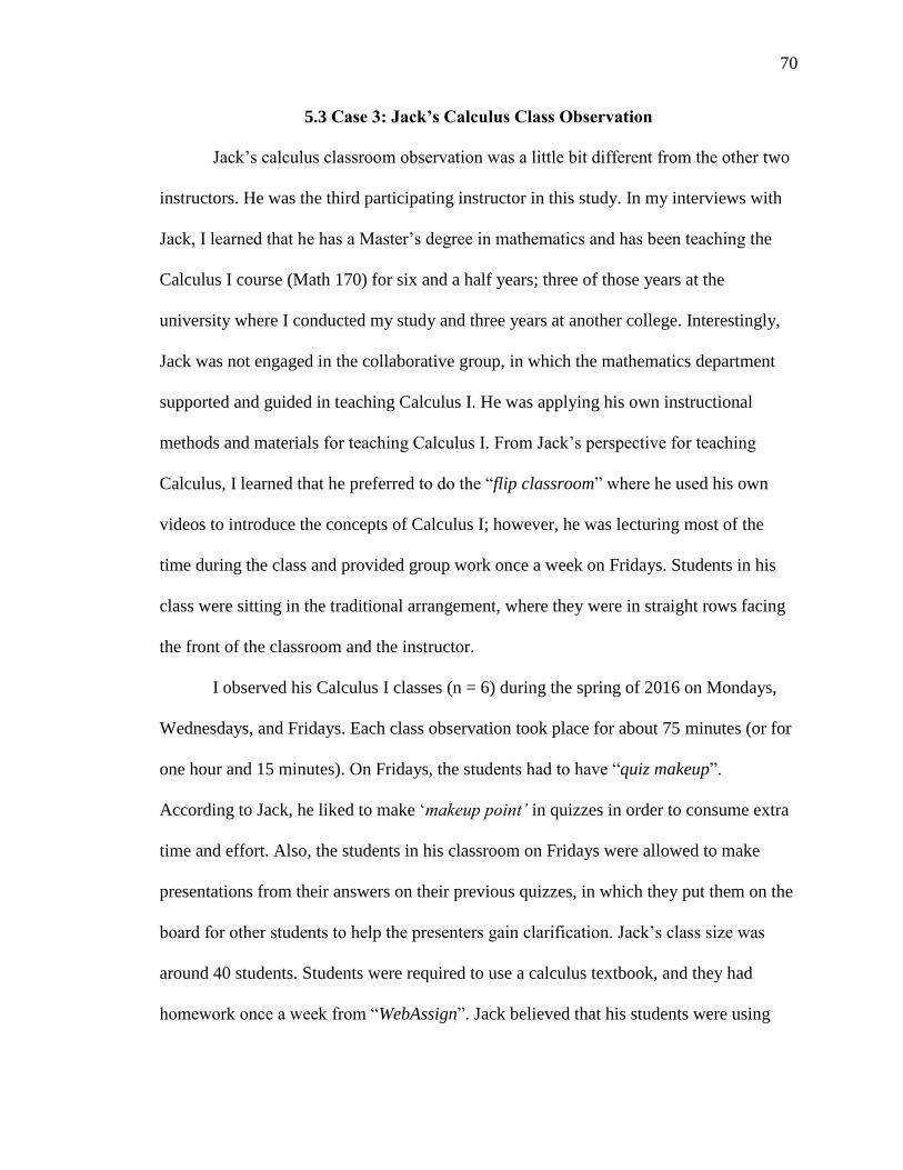
70

5.3 Case 3: Jack’s Calculus Class Observation

Jack’s calculus classroom observation was a little bit different from the other two

instructors. He was the third participating instructor in this study. In my interviews with

Jack, I learned that he has a Master’s degree in mathematics and has been teaching the

Calculus I course (Math 170) for six and a half years; three of those years at the

university where I conducted my study and three years at another college. Interestingly,

Jack was not engaged in the collaborative group, in which the mathematics department

supported and guided in teaching Calculus I. He was applying his own instructional

methods and materials for teaching Calculus I. From Jack’s perspective for teaching

Calculus, I learned that he preferred to do the “flip classroom” where he used his own

videos to introduce the concepts of Calculus I; however, he was lecturing most of the

time during the class and provided group work once a week on Fridays. Students in his

class were sitting in the traditional arrangement, where they were in straight rows facing

the front of the classroom and the instructor.

I observed his Calculus I classes (n = 6) during the spring of 2016 on Mondays,

Wednesdays, and Fridays. Each class observation took place for about 75 minutes (or for

one hour and 15 minutes). On Fridays, the students had to have “quiz makeup”.

According to Jack, he liked to make ‘makeup point’ in quizzes in order to consume extra

time and effort. Also, the students in his classroom on Fridays were allowed to make

presentations from their answers on their previous quizzes, in which they put them on the

board for other students to help the presenters gain clarification. Jack’s class size was

around 40 students. Students were required to use a calculus textbook, and they had

homework once a week from “WebAssign”. Jack believed that his students were using

71

“WebAssign” as “a tool to learn” the concept of calculus, and they worked on required

problems from the textbook. Each lesson labeled as “L” with the lesson number 1, 2...6. I

will provide findings on three lessons from my observations (L1, L2, L3) because Jack’s

other three lessons had different topics other than the derivative concepts focused on this

study. Also, whenever Jack had presentations from students on Fridays, he had more

interactions with individual students, so I could not observe most of the teacher-student

interactions. My observations were mostly based on whole class discussion from his

classes, and showed that the topic of “limit” was not addressed during that time and the

rules of differentiation had previously been addressed. Even though Jack said he was

teaching derivative and integral concepts at the same time, unfortunately, I missed his

classes when he introduced the differentiation rules for taking derivatives from basic

functions (e.g., polynomials…etc.). As a result, my analysis on Jack’s class observations

will focus on how the instructor communicated the concept of the derivative using visual

mediators (graphs and expressions) with words such as “slopes”, “tangent line”,

“position”, “velocity”, and “acceleration” and how he introduced the concepts of anti-

derivatives.

5.3.1 Word Use

In this section, I highlighted the words used in the following quotes from Jack

when he introduced the concept of the derivative, to show how he communicated the

derivative concept using words such as tangent lines, slopes, and velocity connecting

these concepts graphically.

“The calculus concept is very small. There is very little calculus going on here.

Very little calculus. Take a derivative; derivatives of polynomials use the power

rule, that’s it” [observation L1].

72

“You’re going to find all points where the tangent line is horizontal. What’s the

slope of the horizontal line?” [observation L1].

“What’s the slope of the function? What’s the slope of the function, f-prime,

right? [writing on board] That’s the slope of the function?” [observation L1].

“Okay, so the function is f of x [writing on board] equals ten minus x-squared. So,

what’s the slope of the tangent line at any x? Negative 2x, right? So, what’s the

slope of the tangent line on a? [writing on board] Negative 2a. What’s the slope of

the tangent line at negative a? Negative two, negative a, right, which is 2a”

[observation L1].

“So, perpendicular lines have negative reciprocal slopes. [writing on board] Let’s

say this is maybe m1 and m2, slope one and slope two, so, what I’m saying is m1 is

equal to negative one over m2, that’s it. That’s a factor from previous classes.

Okay, so now we can solve this equation for a” [observation L1].

“Teacher: Okay, problem two. The concept here is that the tangent line for a

straight line [writing on board] is itself (always). Okay, so the tangent line, f(x) =

2x + 3, the tangent line for any point on the line is y = 2x + 3. Is itself”

[observation L1].

“Right, that’s what a line is, it’s all points that are related by this equation, where

the y-coordinate is equal to 2 times x plus three. That’s what a line is, right? So,

all of these points, [writing on board] all of these points are on the line 2x + 3. So,

that’s why you put them all in points slope form, just get all, all I’ve done is I’ve

written the same line five times, just in different ways” [observation L1].

“All of this revolves around the fact that the tangent line for a straight line is

itself. It all revolves around that fact. The tangent line for a straight line is itself.

So immediately you can see that the slope is going to be the same …”

[observation L1].

“So the derivative of position is velocity, the derivative of velocity is acceleration,

is acceleration” [observation L2].

“Acceleration [writing on board]…. So acceleration is the, this is just our

definition, acceleration is the derivative of velocity, so acceleration is the slope of

the velocity. We could really see, we could see a lot from this by looking at the

graph, so, now think about slopes of tangent lines. Okay, now are the slopes of

those, are these lines getting steeper or are they getting flatter?”[observation L2].

What’s the derivative of five?

S1: Zero

Teacher: Zero, right? Remember that we can look at that in two different ways,

right, think of the, what’s the slope of the function at five, function at five, the

constant function, the constant function [gestures to board] here. The slope is

zero, you can also look at it like [writing on board]. So, five is the same as five

73

times one, 5 times zero times x to the zero minus one equals zero. Anyway, so the

derivatives and constants are zero, right, ... [observation L2].

In this case, the analysis of word use will focus on the word “derivative” as it was

discussed in contexts of slopes and rate of change using graphs, expressions, notations,

definitions and other visual mediators.

The Derivative Concepts

The derivative concepts were communicated with key words such us “slope”,

“slope of the tangent”, “tangent line” “slope of the function f-prime” and “position,

velocity, acceleration”, and they were addressed using graphs, symbols, and definitions.

For example, when Jack calculated the slope of a tangent line on the graph of a function,

he took the derivative of that function and then solved the equation for x depending on

the type of tangent lines, whether were horizontal, straight, or perpendicular line. Also,

Jack presented the concepts of the derivative in the form of definitions when he

introduced “position, velocity, acceleration” using words and symbols. The findings

focus on how the instructor communicated the concept of derivative as two contexts:

derivatives and anti-derivatives.

In the following analysis, the derivative concept is defined, first, as finding the

equations of a tangent line to a function 𝑓(𝑥) at point (𝑥, 𝑦) using the slopes equation.

For example, mathematically, according to Adams & Rogawski (2015) it is defined that

the “Point-slope form of the line trough P= (a, b) with slope m is the following:

𝑦 − 𝑏 = 𝑚(𝑥 − 𝑎)

Second, derivative concept is defined as finding the area of triangles formed by a

tangent line to a function at given points. Note that what I learned from Jack’s interviews

concerning his teaching of derivatives and integrals (which was about areas) at the same

74

time was that it was often in indirect ways or circuitous ways. Then, third, analyzing the

derivative concepts as “velocity”, according to Jack, from physics, velocity was about

speed and directions, so acceleration was the slope of velocity. My analyses show that the

word use of “slope” appeared in all three areas described above, as well as in how Jack

introduced the concept and used it.

Slope and Slope of the Tangent. The derivative was communicated in the word

use of “slopes” or “slope of tangent line” when the instructor was solving an equation of

‘f-prime’ for a variable x calculating the slope of that tangent line. For example, when

Jack was finding all the points that were on the graph of function 𝑓(𝑥) = 𝑥3 − 𝑥 where

the tangent line was a horizontal line, first Jack took the derivative of that function using

the power rule, 𝑓′(𝑥) = 3𝑥2 − 1, and then he solved that equation for x as the slope of

the horizontal line as zero, which is solving f-prime 3𝑥2 − 1 = 0 for x. In this case, Jack

used the word “slope” to get his students to know the main concept of how they could

solve the problems on a classwork worksheet because the slope of the horizontal line was

zero. He taught them to take the derivative 𝑓’ of the function 𝑓 using differentiation rules

and then wrote the equation in term of 𝑓′(𝑥) = 0 saying: “When the slope of the function

is equal to zero, solve that equation for x using algebra”. In another example, dealing

with a trigonometric function 𝑓(𝑥) = cos(𝑥) + sin(𝑥), Jack found all the points on the

graph of that function where the tangent line was horizontal which meant the slope of the

function, 𝑓′(𝑥) = − sin(𝑥) + cos (𝑥), equals to zero [0 = − sin(𝑥) + cos (𝑥)]. Jack

explained the points using the unit circle [Figure 5.12]:

And so just using that sine and cosine, it’s that right there … zero [writing on

board] … So when is sine x equal cosine x it’s the same as saying when is the, for

what angles, for what angles is the x equal to the y…For what angle is the x-

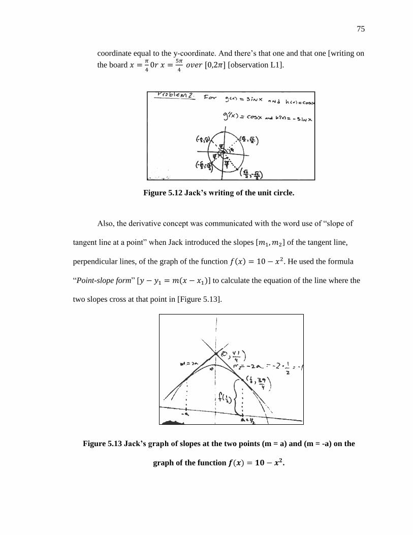
75

coordinate equal to the y-coordinate. And there’s that one and that one [writing on

the board 𝑥 =𝜋

40𝑟 𝑥 =

5𝜋

4 𝑜𝑣𝑒𝑟 [0,2𝜋] [observation L1].

Figure 5.12 Jack’s writing of the unit circle.

Also, the derivative concept was communicated with the word use of “slope of

tangent line at a point” when Jack introduced the slopes [𝑚1, 𝑚2] of the tangent line,

perpendicular lines, of the graph of the function 𝑓(𝑥) = 10 − 𝑥2. He used the formula

“Point-slope form” [𝑦 − 𝑦1 = 𝑚(𝑥 − 𝑥1)] to calculate the equation of the line where the

two slopes cross at that point in [Figure 5.13].

Figure 5.13 Jack’s graph of slopes at the two points (m = a) and (m = -a) on the

graph of the function 𝒇(𝒙) = 𝟏𝟎 − 𝒙𝟐.

76

He explained the concept using the phrase “slope of the tangent line at…”, and he stated:

So, what’s the slope of the tangent line at any x? Negative 2x, right? So, what’s

the slope of the tangent line on a? [writing on board] Negative 2a. What’s the

slope of the tangent line at negative a? Negative two, negative a, right, which is

2a…Now what do we know about the slope of perpendicular lines? Negative

reciprocals, right? So, then we know that the slope of this line is the negative

reciprocal of this line, so we know that 2a is equal to negative one over negative

2a [writing on board]. All right, so, perpendicular lines have negative reciprocal

slopes. [writing on board] Let’s say this is maybe m1 and m2, .. Okay, so now we

can solve this equation for a” [observation L1].

Tangent line and Finding Areas. The derivative concepts were communicated

with the word “tangent line” when finding the area of triangles in a variety of functions

(given in several tasks) by the tangent line to that functions 𝑓(𝑥) at specific points (𝑥, 𝑦),

the x-axis and the y-axis. For instance, the instructor was finding the area of the triangle

shown in Figure 5.14 when calculating the slope of the tangent line at 2 to the function

𝑓(𝑥) =1

𝑥. After he took the derivative of the function f, he wrote 𝑓′(𝑥) = −𝑥−2 = −

1

𝑥2,

and found the slope at 2, he then wrote on the board, 𝑚 = 𝑓′(2) = −1

4. He used the

“point-slope form” to find the equation of the line, 𝑦 −1

2=

1

4(𝑥 − 2). He explained the

previous example by saying:

Ok, so, let’s graph f of x equal 1 over x…we look at the point, we look at 2. Umm

[he is drawing the tangent line on the graph] so the tangent line at 2 forms the

triangle [he is shading the area of the triangle] with x and y axis’s. We want to

find the area of that triangle. What is the area of triangle…[observation L3].

77

Figure 5.14 Jack’s graph of a triangle by tangent line on the graph of 𝒇(𝒙) =𝟏

𝒙.

This example of discussing the derivative concepts as finding area of triangles

tells as about Jack’s approach in teaching Calculus I. As you can see the way he

connected his mathematical ideas of the derivative concepts with context of finding areas

relaying on the ideas of calculating slope of the tangent lines by slopes’ formulas to find

the equations.

Velocity and Slope. The derivative concept was introduced with the ideas of

“velocity” and it was used to articulate the concept that Jack had addressed in class

“(Acceleration) = 𝑎(𝑡) = 𝑣’(𝑡) = (slope of velocity)”, using the word “slope” and

recognizing it from graphs. For example, when he presented the concept in the example

function 𝑣(𝑡) = 𝑡3 − 3𝑡2 + 2𝑡, 0 ≤ 𝑡 ≤ 2, v(t) is in feet/sec.; he was graphing [see

Figure 5.15] the “slopes” of tangent lines and looking for their behavior to see if the lines

were “getting steeper” or getting flatter. He addressed those ideas of slopes with no more

detail. He went on to say:

… So the slope of the steeper lines would be more than the slope of the flatter

lines, right? So the slope is, so the slope is going down, the slope is going down.

Here you can see that we’re going faster here than we are there, right. So, we’re

slowing down, right, we’re slowing down and then we’re, and then, over here,

right, okay, you can see things like that, you know, we’re slowing down, um,

[pause] let’s see now, what happened there, we’re getting steeper, but in the

negative. So, okay, right, anyway, okay, all right, good enough [observation L2].

78

Figure 5.15 Jack's graph of a function 𝒗(𝒕).

Jack’s Example of Anti-derivative

The anti-derivative was introduced using polynomial functions and addressed

with numbers and definitions. Jack started introducing the concept with an example of

“inverse operations” in addition and multiplication, then he gave a definition for anti-

derivative:

… So the overall point here is that [writing on board] the inverse undoes the

original...The same is true for derivatives. More or less true, not entirely true, but

you can think of it that way, it’s fine. The same is true for derivatives. [writing on

board] Say “an” because there’s more than one, right, an anti-derivative of f of x

is a function whose derivative is f of x [observation L2].

Also, the anti-derivative was addressed with numbers and symbols in a table. See

Figures 5.16 (a) and (b) where Jack created a table with columns of functions, their anti-

derivatives, and why.

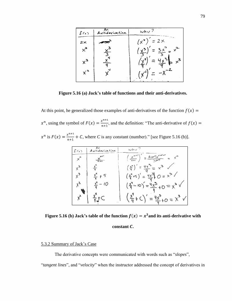
79

Figure 5.16 (a) Jack’s table of functions and their anti-derivatives.

At this point, he generalized those examples of anti-derivatives of the function 𝑓(𝑥) =

𝑥𝑛, using the symbol of 𝐹(𝑥) =𝑥𝑛+1

𝑛+1, and the definition: “The anti-derivative of 𝑓(𝑥) =

𝑥𝑛 is 𝐹(𝑥) =𝑥𝑛+1

𝑛+1+ 𝐶, where C is any constant (number).” [see Figure 5.16 (b)].

Figure 5.16 (b) Jack’s table of the function 𝒇(𝒙) = 𝒙𝟑and its anti-derivative with

constant 𝑪.

5.3.2 Summary of Jack’s Case

The derivative concepts were communicated with words such as “slopes”,

“tangent lines”, and “velocity” when the instructor addressed the concept of derivatives in

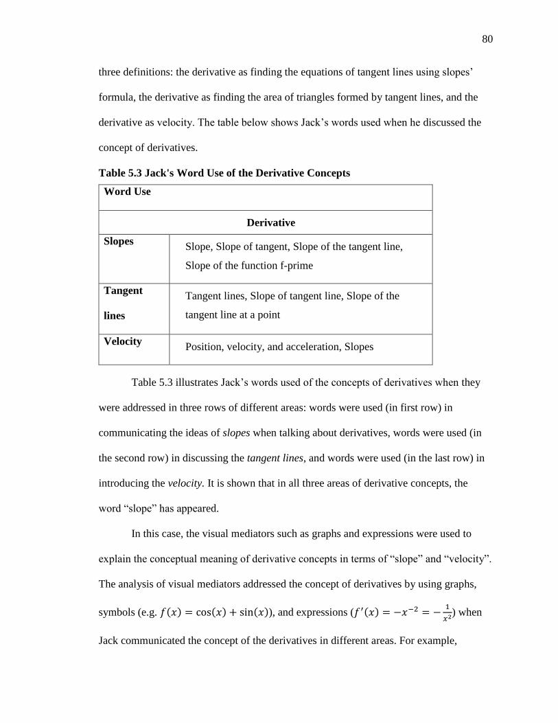
80

three definitions: the derivative as finding the equations of tangent lines using slopes’

formula, the derivative as finding the area of triangles formed by tangent lines, and the

derivative as velocity. The table below shows Jack’s words used when he discussed the

concept of derivatives.

Table 5.3 Jack's Word Use of the Derivative Concepts

Word Use

Derivative

Slopes Slope, Slope of tangent, Slope of the tangent line,

Slope of the function f-prime

Tangent

lines

Tangent lines, Slope of tangent line, Slope of the

tangent line at a point

Velocity Position, velocity, and acceleration, Slopes

Table 5.3 illustrates Jack’s words used of the concepts of derivatives when they

were addressed in three rows of different areas: words were used (in first row) in

communicating the ideas of slopes when talking about derivatives, words were used (in

the second row) in discussing the tangent lines, and words were used (in the last row) in

introducing the velocity. It is shown that in all three areas of derivative concepts, the

word “slope” has appeared.

In this case, the visual mediators such as graphs and expressions were used to

explain the conceptual meaning of derivative concepts in terms of “slope” and “velocity”.

The analysis of visual mediators addressed the concept of derivatives by using graphs,

symbols (e.g. 𝑓(𝑥) = cos(𝑥) + sin(𝑥)), and expressions (𝑓′(𝑥) = −𝑥−2 = −1

𝑥2) when

Jack communicated the concept of the derivatives in different areas. For example,

81

applying the derivative in finding the equations of a tangent line to a function 𝑓(𝑥) at

points using the slopes equation and graphs, and in finding the area of triangles in

different type of given functions by the tangent line of functions 𝑓(𝑥) at specific points

(x, y).

82

CHAPTER SIX: SUMMARY OF FINDINGS

6.1 Discussion

This study investigated how three college instructors communicated the concepts

of derivatives using the concepts of limits, slopes of tangent lines, rates of changes, and

anti-derivatives. In this study, I applied Sfard’s communicational approach to analyze my

data with its two characteristics, word use and visual mediators from calculus classrooms.

I explored three college instructors’ mathematical discourse and the ways they

communicate the concepts of derivative or limit. The findings have highlighted the

instructors’ word use when presenting the concepts of limit and derivative using different

expressions, symbols, and graphs in which they were identified to aid the meaning of the

words used in discussing these concepts. Regarding my research questions, the findings

of the study summarized their instructional approaches and ways instructors

communicate their knowledge in calculus from discourse perspective as follows:

Overall, instructors’ discussions of derivative or limit concepts highlighted the

variation of their word use to communicate these concepts. For example, the

derivative concepts were addressed with various words use such as “velocity”,

“slopes of tangent lines”, and “the limit of the average rate of changes”.

Also, the way that the three instructors represented the derivative concepts were

very different. For example, when Dina was explained the mathematical meaning

of the slopes of tangent lines of given functions while introducing the

differentiation rules, she used graphing illustrations to connect the concepts with

83

expressions and symbols, whereas, Henry communicated his mathematical ideas

of the slopes of the secant lines verbally, when calculating the average rate of

change, and he did not use graphs in introducing the rules. The graphing

illustrations were also found in Jack’s mathematical discourse, when he discussed

the derivative concepts (e.g., solving slope equations).

The differentiation rules were addressed and communicated differently from one

instructor to another. In introducing new rules, only one of the three instructors

(Dina) made explicit connections between the visual mediators, expressions and

graphs of functions, and how the functions affected the slopes of the tangent lines

when graphing the functions of a parent function to a function with multiple

transformations. But Henry had not made connections between graphs and

symbols in introducing differentiation rules; he explained the rules by applying

them in examples, symbolically and numerically.

Instructors’ discourse practices while introducing the anti-derivatives were very

different. They communicated their mathematical ideas of anti-derivative by

definitions and applying the anti-derivative in context of chain rule (as in Henry’s

class), reversing constant and power rule (as in Dina’s class), or creating tables to

generalize definitions in context of power rule (as in Jack’s class).

The two instructors Henry and Dina, who were participating in using the group

materials of teaching Calculus I course in the university, had very different

instructional approaches when they discussed the concept of derivatives or limits.

For example, Dina provided various activities that involved discussions in

graphing explanation, and Henry lectured more and provided similar problems

84

that just asked for finding the derivative algebraically. However, Jack focused on

lecturing and discussing the concepts on the board using visualization meaning,

for example, every time he talked about the derivative concepts, he mainly drew

graphs of the original functions to discuss slopes of tangents line.

Dina and Jack were more eager to use a graph function and its derivative than

Henry was. For example, Dina provided examples of applications using

derivatives to show the derivative behaviors related to graphs of a function f and

the derivative of that function f-prime.

Among the three instructors, Henry and Dina followed the calculus textbook to

introduce the topics in which the concept of the derivatives was taught and

addressed, whereas Jack was applying different teaching approaches as he was

teaching derivative and integral indirectly at the same time. For example, when he

asked questions about finding the area of the triangles formed by tangent lines of

a function at the point (x, y), his discussions with students focused on how they

could find the area using the triangle area formula and slopes formula.

To sum up, this study found that when three instructors taught Calculus I courses,

they all address the concepts of derivative, and always communicated the concepts using

the words “slopes” and “slopes of the tangent lines”. Although the three instructors’

classrooms were observed at different times, the use of the word “slopes” appeared in the

three instructors’ classroom observations in a variety of contexts. As a result, in all of the

three instructors’ classrooms, the derivative concepts were addressed with various words

use such as “velocity”, “slopes of tangent lines”, “the limit of the average rate of

changes”, and were illustrated with graphing explanations besides expressions and

85

symbols as in Jack and Dina’s cases. For example, when Dina was estimating the

derivatives of functions with a graph of those functions, she used the function’s graph to

sketch the derivative’s graph. She communicated her mathematical ideas of derivatives

using graphing behaviors by paying attention to the important points on graphs and

slopes as negative or positive slopes. However, in Jack case, he always used graphs of

original functions when he discussed the ideas of derivatives in terms of velocity, slopes,

or slopes of tangent lines at points. Whereas in Henry case, he rarely used graphs to

communicate his ideas, for example, when he discussed, verbally, the concepts of the

limit of the function 𝑓(𝑡)as average rate of change and instantaneous velocity, then and

computing it.

When the three instructors addressed the derivative and or limit concepts,

sometimes they did not make explicit connections between their use of words and their

visual mediators. For instance, when Henry addressed the concepts of the derivatives

when he was finding the derivative of a function over an interval or at point “a” by

definition, he communicated the concept using words such as “limit of the average rate of

change”, “velocity”, or “instantaneous velocity” without making clear connections with

graphs of the function (visual mediators) and explaining the mathematical meaning of his

words used. However, in Dina’s case, the connections between representations

(graphical, symbolic, and numerical) were found when she explicitly introduced the chain

rule and the product rule. She started her communication about the new rules by graphs

first and then she connected the ideas of the graphs to set up the rules symbolically. After

that, she provided examples to apply these rules numerically using expressions. Also in

the discussion of the differentiation rules in Henry and Dina’s cases, they had different

86

approaches. For example, on one hand, whenever Henry presented the new rules, he

explained them during the lecture time with symbols and numbers providing examples

for applying the new rules, verbally. On the other hand, Dina addressed the

differentiation rules with symbols and graphs to help students connect the concepts of the

new rules, the slopes of the tangents lines, and how the graph of the functions affected the

slope of the tangent lines. She used graphs (visually) in an explicit way to discuss and

differentiate the new rules with the ones that students had learned in previous classes,

connecting that with symbols and numbers by applying the rules.

The derivative concepts were addressed and communicated in variety ways from

the instructors’ calculus classrooms. First, Henry used the same type of warm-up

questions each class time when he introduced the concept of derivatives, after students’

discussion as groups he discussed the warm-up in more detail on the board. Second, Dina

provided a variety of activities when she introduced the derivative concepts using

graphing explanations to communicate her mathematical ideas about the concepts. For

example, on one day, she asked her students to use the graphing calculator to help them

sketch graphs of functions and discuss their answers. Finally, in Jack’s case, he addressed

the concept of derivatives using more algorithmic approaches, and he interpreted the

concepts by the use of graphs and calculations. For instance, when he had computed the

slope of the tangent lines on graphs, he solved the equations using the mathematical

process of the slopes formulas.

Connecting to what Park (2015) had found, some of the key communication skills

are “leaving some fairly difficult steps implicit for the students” (p. 249) in instructors’

teaching and students’ learning. Student difficulties may arise from the instructors’ lack

87

of explicit connections between representations in the classroom discourse. When

instructors provide good communications to guide and direct their mathematical

discussions, students could receive the greatest benefit possible. Moreover, discourse in

the classroom also helps students to have the opportunity to use the mathematical

language including symbols or notations and share their ideas with the teachers (by

asking questions) or with peers (by thinking and reasoning). For example, in the calculus

classroom, the notations of calculus concepts have different meanings, such as ‘f-prime’

or 𝑓′(𝑥), 𝑓 (𝑥), 𝑑𝑓

𝑑𝑥,

𝑑𝑓3

𝑑3𝑓, and

𝑑

𝑑𝑥. Therefore, instructors must put more emphasis and effort

on presenting all the possible notations when talking about the derivative due to its

importance in learning calculus in subsequent classes. Instead, using only common

notations such as f-prime notation, students lack a good sense of using different notations

when they study calculus.

The connections made here between the results from this study and studies found

in teaching and learning of the Calculus I courses emphasize the instructional approaches

and the ways that instructors communicate the course in order to provide a discursive

environment in their classrooms. However, the communication approaches of learning

and teaching mathematics are encouraging the productive roles of instructors to explain

their ideas, and making excellent progress in students’ development (Park, 2015; Sfard,

2008; Nardi, Ryve, Stadler, & Viirman, 2014).

6.2 Limitations

There are few limitations in the study. In this study, I focused on how instructors

teach or communicate the concepts of derivatives or limits. Due to recruitment

challenges, I was not able to collect student data, and it has been helpful to have students’

88

learning data as responses to their instructors’ teaching approaches. Thus, when the

instructors provided group work at the class time, it was challenging to record student-

instructor discussions. Only three instructors participated in this study, and their

instructional approaches were not observed at the same time when they addressed same

topics. The focus of the study, however, was to document and explore the ways in which

the concepts of derivatives and differentiation were communicated by a small group of

college instructors (the three instructors), and how their approaches would help me to

teach the same concepts in the near future. Finally, the instructors’ classroom discourses

and instructional approaches depend on the students’ background because the instructor’s

instructional approaches are influenced by his or her students and will not often clarify

the teaching practices in highly differentiated calculus classes.

6.3 Future Study

This study, in documenting an analysis emphasizing some of the instructors’

mathematical discourses when teaching Calculus I courses, in particular, derivative

concepts, analyzing students’ interactions with their instructors, and focusing on their

understandings of the concepts, could help educators and learners in assessing the

discourse itself. It would be beneficial if we look at how students’ respond to what they

have learned in the classroom and how they communicate their mathematical ideas with

peers and instructors. It would be also important to study different instructors who teach

the same mathematical topics from the same institution, different institutions, and

institutions across different countries. There is a need to promote mathematics education

research in Saudi Arabia in order to increase development in teaching and learning of

mathematics or of any subjects in general. Exploring and investigating mathematics

89

classrooms discourse will benefit both instructors’ and students’ learning. We need to

support our education in how instructors integrate their traditional approaches in teaching

mathematics to the communication approach, discussion, reasoning, thinking, and sharing

ideas with others. This study suggests a mathematical education researcher’s

investigation include the following questions: How do instructors and students

communicate the concepts of derivatives with comprehensive approaches? How does the

use of words in the instructor’s classroom discourse affect a student’s understanding of

particular topics in mathematics, particularly in Calculus I?

90

REFERENCES

Asiala, M., Cottrill, J., Dubinsky, E., & Schwingendorf, K. E. (1997). The development

of students' graphical understanding of the derivative. The Journal of

Mathematical Behavior, 16(4), 399-431.

Ball, D. L. (1993). With an eye on the mathematical horizon: Dilemmas of teaching

elementary school mathematics. The elementary school journal, 373-397.

Bressoud, D.M., Mesa, V., Rasmussen, C. (2014). The calculus student: insights from

the Mathematical Association of America national study. International Journal of

Mathematical Education in Science and Technology .

Bezuidenhout, J. (1998). First‐year university students’ understanding of rate of

change. International Journal of Mathematical Education in Science and

Technology, 29(3), 389-399.

Bode, M., Drane, D., Kolikant, Y. B. D., & Schuller, M. (2009). A clicker approach to

teaching calculus. Notices of the AMS, 56(2), 253-256.

Burns, A. (2014). Calculus Students' Understanding of the Derivative in Relation to the

Vertex of a Quadratic Function.

Cazden, C. B., & Beck, S. W. (2003). Classroom discourse. Handbook of discourse

processes, 165-197.

Clark et al. (1997). Constructing a schema: The case of the chain rule?. The Journal of

Mathematical Behavior, 16(4), 345-364.

91

Ferrara, F., Pratt, D., & Robutti, O., (2006). The role and uses of technologies for the

teaching of algebra and calculus. Handbook of research on the psychology of

mathematics education. past, present and future, 237-274.

Güçler, B. (2013). Examining the discourse on the limit concept in a beginning-level

calculus classroom. Educational Studies in Mathematics,82(3), 439-453.

Gutiérrez, K. D., Sengupta-Irving, T., & Dieckmann, J. (2010). Developing a

mathematical vision. Language and mathematics education: Multiple perspectives

and directions for research, 29-71.

Hardy, N. (2009). Students’ Perceptions of Institutional Practices: The case of Limits of

Functions in College level Calculus Courses. Educational Studies in Mathematics,

72(3): 341-358

Habre, S., & Abboud, M. (2006). Students’ conceptual understanding of a function and

its derivative in an experimental calculus course. The Journal of Mathematical

Behavior, 25(1), 57-72.

Kendal, M., & Stacey, K. (2000). Acquiring the concept of derivative: Teaching and

learning with multiple representations and CAS. DOCUMENT RESUME, 135.

Kendal, M., & Stacey, K. (2003). Tracing learning of three representations with the

differentiation competency framework. Mathematics Education Resea

Journal, 15(1), 22-41.

Leinhardt, G., Zaslavsky, O., & Stein, M. K. (1990). Functions, graphs, and graphing:

Tasks, learning, and teaching. Review of educational research, 60(1), 1-64.

Moschkovich, J. N. (2010). Language and mathematics education: Multiple perspectives

and directions for research. IAP.

92

Nardi, E., Ryve, A., Stadler, E., & Viirman, O. (2014). Commognitive analyses of the

learning and teaching of mathematics at university level: the case of discursive

shifts in the study of calculus. Research in Mathematics Education,16(2), 182-

198.

Orhun, N. (2012). Graphical Understanding in Mathematics Education: Derivative

Functions and Students’ Difficulties. Procedia-Social and Behavioral

Sciences, 55, 679-684.

Park, J. (2015). Is the derivative a function? If so, how do we teach it? Educational

Studies in Mathematics, 89(2), 233-250.

Park, J. (2016). Communicational approach to study textbook discourse on the

derivative. Educational Studies in Mathematics, 91, 395-421.

Porter, M. K., & Masingila, J. O. (2000). Examining the effects of writing on conceptual

and procedural knowledge in calculus. Educational Studies in

Mathematics, 42(2), 165-177.

Rogawski, J. and Adams, C. (2015, 2012, 2008). Calculus

Schleppegrell, M. J. (2010). Language in Mathematics Teaching and Learning. In Judith,

N. M. (Eds.), Language and Mathematics Education: Multiple perspectives and

directions for research (73-112).

Sfard, A. (2008). Introduction to Thinking as communicating. The Mathematics

Enthusiast, 5(2), 429-436.

Sfard, A. (2008). Thinking as communicating: Human development, the growth of

discourses, and mathematizing. Cambridge University Press.

93

Tall, D. (1992). Students’ Difficulties in Calculus. Published in Proceedings of Working

Group 3 on Students’ Difficulties in Calculus, ICME-7 1992, Québec, Canada,

(1993), 13–28. ISBN 2 920916 23 8.

Tall, D (1997) Function and Calculus. A. J Bishop et al (Eds,). International Handbook

of Mathematics Education, 289-325, Dordrecht: Kluwer.

Tall, D., Smith, D., & Piez, C. (2008). Technology and Calculus. Research on

Technology and the Teaching and Learning of Mathematics, 1, 207-258.

Tall, D & Vinner, S. (1981). Concept Image and Concept Definition in Mathematics with

particular reference to Limits and Continuity.

Walshaw, M., & Anthony, G. (2008). The teacher’s role in classroom discourse: A review of

recent research into mathematics classrooms. Review of educational research, 78(3),

516-551.

Zandieh, M. J. (1997). The Evolution of Student Understanding of the Concept of

Derivative.

94

APPENDIX A

95

Instructor Interview Protocol

1- How long have you been teaching Calculus I? And at BSU?

2- As an instructor, what are the challenges (if any) in teaching Calculus I? What

about in teaching derivatives and differentiation rule?

3- As an instructor, what are the challenges (if any) do you anticipate in learning

Calculus I? What about in learning derivatives and differentiation rule?

4- What are the instructional methods do you use when teaching derivatives and

differentiation rule?

5- Can you describe a typical Math 170 class meeting in your classroom such as the

setting, the design of the class, etc.?

6- When teaching differentiation rules and derivatives, what are your instructional

plans?

7- Do you usually incorporate technology such as laptops, computer Apps,

calculators, … etc.) when teaching Math 170? Do you plan to use technology

when teaching derivatives and differentiation rule? Can you say more about how

the technology will be used in teaching the topics?

8- Have you participated in any workshops or training that are related to teaching in

Calculus? If so, what are they? Are they helpful?

Research for this project was conducted under the review of the Institutional Review

Board at Boise State University, Prototcol #020-SB15-174.