Inversion of Time domain 3D Electromagnetic data

Eldad Haber∗ Douglas W. Oldenburg R. Shekhtman†

September 12, 2005

Abstract

Inversion of 3D time-domain electromagnetic data is a challenging problem due toits size and nonlinearity. In this paper we present a general formulation for invert-ing time domain electromagnetic data. To overcome the difficulties we combine anddevelop many computational tools including: Quasi-Newton methods and precondi-tioners, artificial time stepping and source terms. This combination allows us to dealwith realistic geophysical problems.

keywords: Electromagnetic, Time-Domain, Inversion

1 Introduction

In this paper we develop an inversion methodology for large scale parameter identificationproblems which evolve from 3D time domain electromagnetic simulations. This type ofproblem is of major interest in geophysics, medical imaging and non-destructive testing; seefor example [29, 27, 10, 6, 30, 16, 7] and references therein. The forward model consists ofMaxwell’s equations in time where the permeability is fixed but electrical conductivity can behighly discontinuous. The parameter regimes considered give rise to highly stiff problems inthe time domain. The goal of the inversion is to recover the conductivity given measurementsof the electric and/or magnetic fields.

There are many practical challenges to solving the inverse problem. First, a fast, accurateand reliable algorithm for 3D forward modeling is required. Second, the sensitivities for suchproblems are too numerous to be formed or stored in a reasonable amount of time andspace. Finally, finding the minimum of the objective function obtained by matching thedata and incorporating a priori information on the conductivity field can be difficult due tothe nonlinearity of the problem.

Further difficulties are often confronted when trying to invert a particular data-set. Forexample, in geophysical surveys such as large-loop UTEM surveys or CSAMT surveys, the

∗Department of Mathematics and Computer Science, Emory University, Atlanta, GA.†UBC-Geophysical Inversion Facility, Department of Earth and Ocean Sciences, University of British

Columbia, Vancouver, B.C., V6T 1Z4, Canada.

1

transmitter may be some distance away from the area of interest. Discretizing a spatialvolume that includes the transmitter and receivers can result in an excessively large problem.Also, most transmitter waveforms have an on-time and off-time and the ideal scenario is thatelectromagnetic fields have completely decayed away before the next waveform begins. Inconductive environments however the decay time might extend for a couple of periods of theinput waveform. Modelling the field data then requires an extended source that consists of afew repetitions of the waveform. This increases the time for forward modelling, or effectivelythe size of our space-time inverse problem.

A main impediment to inverting time domain electromagnetic data is the size of theproblem and the number of computations to be carried out. To be more specific, assumethat the forward problem (in continuous space) is written in the form

A(m)u− b = 0 (1.1)

where A(m) is a version of Maxwell’s equations (including boundary conditions), m = log(σ)is the log conductivity, u stands for the fields and b represents sources and boundary values.We assume for simplicity of exposition that A is invertible for any relevant m, that is, thereis a unique solution to the forward problem.

In the inverse problem we measure some function of the fields and desire to recover themodel m. Let us write the measured data as

dobs = Qu + ε (1.2)

whereQ is a measurement operator which projects the fields (or their derivatives or integrals)onto the measurement locations in 3D space and time, and ε is the measurement noise. Thedata are finite in number and contaminated with noise, and therefore there is no uniquesolution. To obtain a single model which depends stably on the data we incorporate a-priori information and formulate the inverse problem (in continuous space) as a constrainedoptimization problem of the form

minm,u

1

2‖Qu− dobs‖2 + βR(m) (1.3)

subject to A(m)u− b = 0.

Here, β > 0 is the regularization parameter, and R(·) is a regularization operator reflectingour a-priori information. Typically, we know that m is a piecewise smooth function overthe spatial domain Ω in 3D, so we assume that R(·) involves some norm of ∇m over Ω,e.g., weighted L2 or L1 or a Huber combination [24, 12]. This type of regularization can bewritten as

R(m) =

∫

Ω

ρ(|∇m|) dx + γ1

2

∫

∂Ω

(m−mref )2dx (1.4)

where ρ is given by the Huber function and m0 is some background reference model andγ is a user-specified constant that adjusts the relative influence of the two terms in the

2

regularization functional. The choice of this functional ensures that the weak form hasDirichlet boundary conditions and that in regions far away from where we have data, themodel converges to a known background. This choice also guaranties that the Hessian of theregularizer is invertible.

Next, the problem (1.3) is discretized using some finite volume method over a finite gridrepresenting the domain in space and time. This yields the finite dimensional optimizationproblem

minm,u

1

2‖Qu− dobs‖2 + βR(m) (1.5)

subject to A(m)u− b = 0,

where u, m and q are grid functions ordered as vectors and correspond to their continuouscounterparts above, and Q and A are large, sparse matrices. The matrix A depends on mand is nonsingular. The discrete regularization function has the form

R(m) = e>ρ(|∇hm|) + γ||W (m−mref ||2 (1.6)

where ∇h is the discrete gradient operator and e is a vector of ones.In previous work [21] we have used an inexact, all-at-once methodology [5, 17, 3] to solve

(1.5), solving the forward problem and the inverse problem simultaneously in one iterativeprocess. While this approach can be highly efficient, it requires storage of all time-spacehistory of the fields.

In this work we aim to deal with very large scale problems and multiple sources. For suchproblems one cannot store all the fields on computer hardware that is currently available tous, and we therefore turn to other avenues for the solution of the problem. A simple way toreduce storage is to use a reduced space method, which eliminates Maxwell’s equations, andsolves the unconstrained optimization problem

minm

1

2‖QA(m)−1b− dobs‖2 + βR(m). (1.7)

This leads to the Euler-Lagrange system

g(m) = J(m)>(QA(m)−1b− dobs) + βRm(m) = 0 (1.8)

where

J(m) = −QA(m)−1G(m)

G(m) =∂[A(m)u]

∂m.

and J(m) is the sensitivity matrix (see [20] for derivation) and Rm(m) = ∂R∂m

.We search for an m that solves (1.8). The evaluation of g(m) involves a number of

computations. To calculate Rm(m) we use the chain rule

Rm(m) = ∇>h ρ′(|∇hm|)∇hm + γW>W (m−mref ).

3

Also, the forward problem must be solved to generate predicted data, and calculating theaction of J(m)> on a vector requires the solution of the adjoint problem. If a gradient descenttype method is used to solve (1.8) then each iteration requires the solution of a forward andadjoint problem which means solving Maxwell’s equations forward and backward in time. Inaddition a line search involving forward modeling must be carried out.

Newton-type methods are generally far superior to descent methods when solving (1.8).If a Gauss-Newton method is used, then at each iteration we solve the linear (but dense)system

(J(m)>J(m) + βRmm)s = −g(m) (1.9)

where s is a model perturbation. This system is never formed explicitly but is solved usingconjugate gradient (CG) methods. At each CG iteration J(m) and J(m)> are applied to avector and hence a forward and adjoint problem must be solved. Even with reasonably goodpreconditioners, a few tens of CG iterations are likely required to get a good estimate of s.This results in many forward modellings and hence the cost of a Newton-CG algorithm isalso too high. We therefore turn to Quasi-Newton techniques.

In a quasi-Newton method we solve a system

B(m)s = −g(m) (1.10)

where B is an approximation to the Hessian. One of the most successful methods for un-constrained optimization is the limited memory BFGS (L-BFGS) method [26]. In a BFGSmethod either B or it’s inverse, B−1, is built up through successive iterations. The maincomputations at each iteration are construction of the gradient and performing a line search.The constituent vectors for constructing B need to be stored. The limited memory versionof BFGS addresses this issue. While the method is highly attractive for inverse problems,naive implementation of L-BFGS usually fails (see [15] for details).

In this paper we propose a practical strategy that combines the strengths of Gauss-Newton and quasi-Newton approaches. Firstly, we alter the usual Tikhonov methodology touse an iterated Tikhonov approach that partially overcomes difficulties in solving the opti-mization problem when the regularization parameter is small. We then explore a particularimplementation of L-BFGS and use the constructed approximate inverse Hessian as a pre-conditioner for the Gauss-Newton iteration. This substantially reduces the number of CGiterations in solving (1.9). We also present strategies for dealing with some of the practicalissues mentioned earlier. In particular we introduce a source correction procedure that allowsus to reduce the spatial volume of the region to be inverted and ameliorates discretizationerrors. We also introduce a technique to work with problems that have an extended timesource.

The paper is divided as follows. In Section 2 we describe the solution of the forwardproblem. In Section 3 we discuss how to modify the right hand side of the forward problemsuch that the size of the discretized domain is smaller. In Section 4 we discuss the overallapproach for the solution of the problem and motivate the use of Quasi-Newton methods.In Section 5 we discuss efficient implementation of Quasi-Newton methods. In Section 6 we

4

discuss how to deal with extended waveforms source-signals. We give numerous examples inSection 7 and the paper is summarized in Section 8.

2 Solution of the forward problem

In this section we present our forward problem, Maxwell’s equations, and discuss solutionprocedures suitable for the parameter regimes of interest. Most, but not all of the presentdevelopment follows our previous work [18, 16, 21].

2.1 Reformulation and discretization

The time-dependent Maxwell equations can be written as

∇× E + µ∂H

∂t= 0, (2.11a)

∇× H− σE− ε∂E

∂t= sr(t) (2.11b)

over a domain Ω × [0, tf ], where E and H are the electric and magnetic fields, µ is thepermeability, σ is the conductivity, ε is the permittivity and sr is a source. The equationsare given with boundary and initial conditions:

n×H = 0 (2.11c)

H(0,x) = H0 (2.11d)

E(0,x) = 0 (2.11e)

although other boundary and initial conditions could be used.Since the equations are very stiff [4, 21] we turn to implicit methods, and use a BDF

(Backward Difference Formula) type method. For the work here we choose the simplest,lowest order member of both these families of stiff integrators, namely, the backward Eulermethod. This allows us to simplify the presentation, however we have also implemented aBDF(2) integrator and the reader is referred to [19, 21, 23].

Semi-discretizing (2.11), (2.11c) over a time step [tn, tn+1] yields the equations

∇× En+1 + αnµHn+1 = αnHn in Ω (2.12a)

∇× Hn+1 − (σ + αnε)En+1 = sn+1r − αnεEn in Ω (2.12b)

n×Hn+1 = 0 on ∂Ω. (2.12c)

where αn = (tn+1 − tn)−1. The superscripts in (2.12) denote the time level, with solutionquantities at n + 1 being unknown while those at n are known.

Rather than working with the fields En+1 and Hn+1 we first eliminate Hn+1 from (2.12)

Hn+1 = Hn − (αµ)−1∇× En+1.

5

Substituting, we obtain an equation for En+1

∇× µ−1∇× En+1 + ασEn+1 + α2εEn+1 = α(∇× Hn + αεEn − s). (2.13)

As discussed in [18, 16] the discretization of the system (2.13) is difficult to solve usingiterative methods. Introducing the potentials A, φ to write E = A +∇φ we get

(∇× µ−1∇× −∇µ−1∇· )A + α(σ + αε)(A +∇φ)n+1 = (2.14)

α(∇× Hn + αεEn − s)

∇ · (σ + αε)(A +∇φ)n+1 = α∇ · εEn −∇ · s (2.15)

For ease of notation we introduce σ = σ + αε. The continuous equations are discretizedin space using a finite volume technique on a staggered grid. See (see details in [18, 16, 21]).Variables A and E are defined at the center of cell faces, H is defined on the edges, and φin the cell centers. Upon discretization we obtain

(Lµ + αMσ αMσG

DMσ DMσG

)(Aφ

)=

(α(CeH

n + αεEn − s)εαDEn −Ds

)(2.16)

whereLµ = CeMµCf −GM c

µD

and the matrices Ce, Cf , G and D are respectively the discretizations of the curl on the edgesand faces, the gradient and the divergence. The matrix Mσ is a discretization of σ + αε onthe cell faces. It is composed of harmonic averages of σ for the two cells in contact at a face.The matrix Mµ consists of arithmetic averages of the permeability for cells adjacent to anedge.

This linear system can be solved using standard iterative methods [28] and effectivescaleable preconditioners can be designed for it [18, 1].

2.2 Summary - the forward problem

In many applications we are concerned with multiple sources and with multiple time steps.For solving the inverse problem it is useful to formulate the forward problem as a singleequation (see for example Section 1).

We note that it is possible to rewrite the system as a lower block bidiagonal system forA, φ and H of the form

A(m)u =

A1(m)B2 A2(m)

B3 A3(m). . . . . .

Bs As(m)

u1

u2...

us

=

q1

q2...

qs

(2.17)

6

where

un =

An

φn

Hn

, An(m) =

Lµ + αnMσ αnMσ∇h 0∇h · Mσ ∇h · Mσ∇h 0

α−1n M−1

µ ∇h× 0 I

qn =

−αnsr

n

−∇h · snr

0

, Bn =

−εα2n −εα2

n∇h −αn∇Th×

−∇h · εαn −∇h · εαn∇h 00 0 −I

.

In the case of multiple sources we obtain a block diagonal system where each blockhas the same structure as (2.17). Note that only the diagonal blocks in (2.17) depend onthe conductivity. Also, once we have an efficient solver for one block Ak(m), solving theforward problem (2.17) is straightforward (with the cost of solution increasing by a factor ofs compared to the cost of solving for one block).

3 Corrective Sources

Our boundary condition requires the domain to be large enough such that the magnetic fieldsare dramatically reduced. This may require that a very large domain be modeled. This isespecially true if the sources are far from the receivers, as they are in many EM surveys.

To make the problem tractable we introduce a correction procedure which has manyelements of a primary/secondary field formulation. The methodology can be used to reducethe size of the problem and also to provide a first order correction for discretization errors.We first write the steps in a generic manner and then show how this is implemented in thetime domain equations.

Let A denote a general operator which depends upon m, our physical property of interest(i.e. electrical conductivity), u is a field, and q is a source. m, u, q are all functions with arelationship

A(m)u = q (3.18)

The above equations are also provided with boundary conditions. Analytic, or quasi-analytic, solutions are available only for simple situations, for example, finding the fields ina half-space due to an electric or magnetic source. For realistically complicated earth modelswe obtain a numerical solution by solving a discrete system

Ah(m)uh = qh (3.19)

where Ah is a matrix that results from the discretization of A, uh is a vector of (discrete)field values, and qh is a vector that contains the discretized source and boundary conditions.

Let m0 be a model for which we can generate an exact solution to equation (3.18) andlet the discrete field values be u(m0). It is unlikely that u(m0) is an exact solution for thediscrete equations (3.19). The residual is

Ah(m0)u(m0)− qh = s. (3.20)

7

This discrepancy can be regarded as a corrective source and added to the discrete equations.We therefore solve

Ah(m)uh = qh + s. (3.21)

It is straightforward to show that when m = m0 the solution of the discrete equationsuh = u(m0). So the numerical solution is equal to the ”exact” solution for our referenceproblem. The above correction can be used for the following two modeling problems.

1. Discretization errors: The corrective source is a set of currents that compensate forthe differences between the discrete and continuous models for a specific conductivity.This is particularly useful for dealing with the current source. In geophysical fieldapplications the source current is carried by a small wire, whereas in the discreteformulations the current is assumed to be distributed through the face of a cell. If areceiver is close to a transmitter, the difference in fields can be significant.

2. Reducing the size of the problem. In CSAMT problems, or large loop UTEM surveys,the data are acquired in a region that is significantly away from the source. Our dataarea, and region of interest, is much smaller than the volume that contains the trans-mitter and receivers. If the discretized volume is outside the region of the transmitter,the corrective- source will primarily be currents on the boundary of the volume.

The corrective sources provide the needed compensation for a specific conductivity. Wehave no mathematical procedure for evaluating how well the correction terms work when theconductivity changes significantly from m0. However, in the problem of reducing the volume,it is expected that if a reasonable estimate of the large-scale background conductivity isknown, and if the secondary fields for the structure inside our reduced volume are smallon the outside of the reduced volume, then our procedure should work well. Numericalexperiments substantiate this.

We now apply the above methodology to our time domain problem. Assume we havecalculated the flux Jn

0 and the magnetic field Hn0 n = 1..N , that correspond to the conduc-

tivity σ0 and the source s. This can be done by analytic formulas [32] or by using 1D codesthat allow for the calculation of highly accurate fields given a simplified earth model. Thecorresponding (discrete) electric field is

En0 = M−1

σ0Jn

0

Our basic equation is (2.13) and thus the source for time tn+1 is

s0 = CeMµCfEn+10 + αMσ0E

n+10 + α2εEn+1

0 − α(CeHn0 + αεEn

0 − s) (3.22)

Using the potentials we therefore have

(Lµ + αMσ αMσG

DMσ DMσG

)(Aφ

)=

(s0 + α(CeH

n + αεEn − s)Ds0 + αDεEn −Ds

)(3.23)

8

Note that upon using s0 in (2.13), and the equivalent A − φ formula (3.23) with thebackground conductivity σ0, we obtain the fields E0 and H0. The right hand side of theequation is zero (up to discretization errors) where there are no electric or magnetic sources.However, the right hand side is different from zero on the boundary of our domain. This canbe thought of an artificial source which emulates the source influence on a finite grid.

Numerical experiments show that the formulation (3.23) allow us to dramatically reducethe volume under consideration without sacrificing accuracy.

4 Inversion Framework

4.1 Inversion algorithms

As discussed in the introduction we aim to solve the minimization problem (1.7). Thereis one further complication when solving the optimization problem because, in general, theregularization parameter is unknown a-priori. Therefore, we need to solve the optimizationproblem a few times for different regularization parameters. The ”optimal” regularizationparameter has to be chosen using an appropriate criteria such as discrepancy principle [27]or GCV [22, 31]. A general sketch of the algorithm that achieves this goal is as follows

Algorithm 1 Tikhonov Inversion algorithm:[m,β] ← INV(m0, β0);

while true dogiven β approximately solve (1.7) for mβ with starting guess m0

if mβ fulfills chosen stopping criteria thenbreak;

end ifupdate β, set m0 ← mβ

end while

Algorithm 1 is a common implementation of Tikhonov regularization. However solvingthe optimization problem (1.7) becomes increasingly harder as the regularization parame-ter approaches zero. One way to alleviate this difficulty is to use an iterated Tikhonovregularization [11].

The use of iterated Tikhonov for nonlinear problems has been analyzed in [8] and it isknown to give similar results to the Tikhonov regularization. We will further explore theuse of Iterated Tikhonov regularization for geophysical inverse problems in a future paper,however, for now we discuss the basic theoretical properties of the method.

The iterated Tikhonov regularization is based on the observation that the nonlinearequation (1.8) can be rewritten as

m−m0

τ= R−1

mmJ(m)>(dobs −QA(m)−1b) (4.24)

9

where m0 = 0 and τ = β−1. Equation (4.24) is a single backward Euler step of the nonlinearODE

m = R−1mmJ(m)>(dobs −QA(m)−1b) (4.25)

m(0) = 0 (4.26)

This implies that methods other than a single backward Euler method can be used. Forexample, in the classical implementation of the Iterated Tikhonov Regularization method afew backward Euler steps are taken with the same regularization parameter (or time step).Thus we solve the following sequence of problems with the same regularization parameterbut with a changing reference model mref .

minm

1

2‖QA(m)−1b− dobs‖2 + βkR(m−mrefk

) (4.27)

It can be shown under mild assumptions that if we set mref to the solution of the kth

problem, then the algorithm reduces the data misfit at each iteration. A sketch of theiterated Tikhonov regularization is as follows

Algorithm 2 Iterated Tikhonov Inversion algorithm:[m,β] ← ITINV(mref , β);

while true dogiven the reference model mref approximately solve (4.27) for mk with starting guessmref

if mk fulfills chosen stopping criteria thenbreak;

end ifupdate reference model, set mref ← mk

end while

It is also possible to combine algorithms and change the regularization parameter as wellas the reference model. In this approach both the regularization parameter and the referencemodel change at each iteration. This leads to faster reduction in the misfit.

Using an iterative regularization has one main advantage. The regularization parameterβ used at each iteration is larger than the equivalent one used for classical Tikhonov regular-ization. This can be advantageous since the convergence of the linear solver at each iterationis highly dependent on the size of the regularization parameter. On the other hand, thereare some disadvantages to the iterative regularization approach. The main one is that it isdifficult to take advantage of solving problems on coarser grids [2]. Our code implementsboth strategies for the solution of the problem.

5 Efficient implementation of Quasi-Newton methods

Irrespective of whether we use a Tikhonov or iterated Tikhonov approach, an essential com-putation is the solution of equations (1.9). These will be solved with a CG solver and the

10

efficacy of solution depends strongly on the preconditioner. In previous work [21] we usedthe matrix M = (0.1I + βW T W ) as a preconditioner. This worked well for large β butwas less effective as β decreased. To improve computational efficiency we need to find abetter approximation to the Hessian matrix (J>J + βRmm). We will use Quasi-Newtontechniques to construct an approximation to the inverse Hessian and use that matrix asa preconditioner. As a prelude we discuss Quasi-Newton methods for the solution of theoptimization problems (1.7) and (4.27). We start by introducing some notation, review theL-BFGS method and discuss important points in it’s implementation.

For a fixed regularization parameter β and reference model mref , given two approximatesolutions mj and mj+1 and the two corresponding gradients gj and gj+1, we define, as isusual in Quasi-Newton methods,

sj = mj+1 −mj

yj = gj+1 − gj.

The usual Secant Condition [9, 26] is

Hjsj = yj (5.28)

where Hj is an approximation to the Hessian. In our case the Hessian has the structure

Hj = J>j Jj + Bj + βRmm

where Rmm is a known, sparse, easy-to-evaluate matrix and

Cj := J>j Jj + Bj

is a dense hard-to-evaluate matrix which corresponds to a compact operator [11]. CommonQuasi-Newton methods do not make use of the known part and evaluate the whole Hessian.However, we would like to use the known information about the Hessian.

To do that, we also note that for the applications we consider here, we have an ex-plicit knowledge of the gradients with respect to the data objective function and the modelobjective function

gd(m) = J(m)>(QA(m)−1b− dobs) (5.29a)

gm(m) = βRm(m; mref). (5.29b)

Using the separability of the objective function and the gradient we now discuss approxima-tions to the Hessian.

In the BFGS method one uses equation (5.28) to approximate the inverse of the Hessiandirectly. The standard BFGS update is (see [9, 26])

H−1k+1 = (I − γksky

>k )H−1

k (I − γkyks>k ) + γksks

>k (5.30)

where γk = (s>k yk)−1. In the L-BFGS method only a limited number of vectors are kept

and the matrix H, or H−1, is never generated explicitly. The vectors mj, gj j = 1, . . . `

11

are saved and an inverse-Hessian matrix vector product can be calculated using recursion(see [25] for details).

Although it is possible to use the L-BFGS methods directly. As discussed in [13], if thematrix Rmm is constant (as when the regularization is quadratic) it is crucial to initiate theHessian with βRmm. This implies that when calculating the inverse-Hessian times a vectorone needs to calculate the product v = R−1

mmw. This can be done by the solution of thesystem Rmmv = w, which can be achieved directly, or using a multigrid method [14].

However, there are a few difficulties when using L-BFGS for the solution of our particularproblem. Consider the L-BFGS solver imbedded into the algorithms 1, 2. When solving twoadjacent problems, with a different regularization parameter or a different reference model,the gradients of the previous functions cannot be used. This implies that a standard imple-mentation of L-BFGS requires restarting the process ignoring all (potentially useful) previousinformation. We therefore suggest a variant which makes use of previous approximations tothe solution.

Assume we are in iteration ` of a BFGS algorithm with a reference model mrefk and aregularization parameter βk and that we have the vectors

gi = gdi + βkRm(mi; mrefk), mi i = 1 . . . `

Now assume that the regularizer part has changed either because βk or mrefk has changedto βk+1 and mrefk+1

. Straight forward implementation of BFGS requires we restart theprocess ignoring information we have previously collected. However, we can circumvent thisand define the following new set of vectors

gi = gdi + βk+1Rm(mi; mrefk+1

), mi i = 1 . . . ` (5.31)

It is clear that the set of vectors gi i = 1, . . . , ` are the gradients of the modified objectivefunction which corresponds to previous models m1, . . . , m`. We can therefore use thesevectors to generate a new BFGS approximation to the Hessian. Note that for the class ofregularization we consider here, Rm(mi; mrefk+1

) can be calculated in linear time.When using the new BFGS vectors we must test the Quasi-Newton condition, y>j sj ≥ 0.

If this condition does not apply to the new Quasi-Newton vectors then we simply drop thecorresponding pair.

In the L-BFGS method one chooses a maximum number of vectors, (lmax, to be used.The convergence rate increases with lmax but so will storage requirements. Thus lmax will beproblem and machine dependent.

Although the optimization problem could be solved directly with L-BFGS, we have foundthat it gave poor performance. We suspect that for small regularization parameters manyBFGS vectors are needed in order to obtain a good approximation to the Hessian. Neverthe-less, the BFGS approximation to the Hessian can still perform very well as a preconditionerfor the GN system. This is the role it plays here.

12

6 Working with extended waveforms

Most transmitter waveforms have an on-time and off-time and the ideal scenario is thatelectromagnetic fields have completely decayed away before the next waveform begins. Inconductive environments however the decay time might extend for a couple of periods of theinput waveform. Modeling the field data then requires an extended time source that consistsof a few repetitions of the waveform. As a example, consider a conductive sphere buriedin a low conductivity background. Suppose that the sphere has a late-time decay constantτ = 100msec. The waveform is a half-sinusoid pulse followed by an off-time. The data areacquired in the off-time and stacked over many periods. The final data set is assumed tobe the steady state values. If the fundamental frequency of the transmitter is 10Hz, thennumerical experience shows that at least three cycles of a waveform need to be modeledbefore an approximate steady state solution is reached. Rather than carrying out this timestepping in all forward modelings for the inverse problem we now suggest a new method todeal with this difficulty.

Assume that the conductivity structure of the earth is known and that we can run thefull forward problem with this conductivity structure. Let ue be the field that correspondsto time te, which is the time after a few waveforms and assume that the magnetic field ismeasured only at time equal to, or larger than, te. We rewrite the system as

A(m)u =

A1(m)B2 A2(m)

. . . . . .

Be Ae(m). . . . . .

Bs As(m)

u1

u2...ue...us

=

q1

q2...qe...qs

(6.32)

For the inversion we are interested only in fields at times te and later. But to computethe field at te we need to know ut−1, the field at te−1. If this were known then we could solvea much smaller forward problem

Aredured =

Ae(m). . . . . .

Bs As(m)

ue...us

=

qe −Beue−1...qs

(6.33)

The problem is that the field ue−1 is not known unless we had previously performed a fullforward modeling and computed and stored it. Then, if the forward modeling for times te andbeyond are needed, we can avoid computing all previous fields and use the forward problem(6.33) instead of the full forward problem (6.32). This saves many of the computations.

However, in the course of the inversion process, we do not compute the same field twice.We need to compute the forward problem only after we update the model. Fortunately,since the PDE is stiff, if the change to the model is small then the change to the fields isexponentially smaller. Thus, for small changes in the model, we are able to obtain a good

13

enough solution to our forward problem even with the fields ue−1 computed from a near-bymodel. This observation motivates the following idea. Replace the forward modeling matrixA(m) with Ared and guess the fields at time ue−1. This implies that not only is the forwardproblem easier to solve, but the gradients and the product of the sensitivity matrix with avector are also cheaper to compute. However, we must keep track of ue−1 and update it asm changes. This idea can be summarized by the following algorithm.

Algorithm 3 Gauss-Newton Time Domain Inversion with Approximate Initial Conditions:[m] ← GNNV(mref , β);

Initialize: set m = mref and choose β.while true do

[1] Compute the forward problem and store ue−1

[2] Compute the gradient (equation (1.8)) using the reduced forward modeling Ared

[3] Compute the Gauss-Newton correction s using equation (1.9) with the reduced for-ward modeling Ared

[4] Update the model, mk+1 ← mk +αs where α is a line search parameter to guaranteereduction in the objective function.if mk+1 fulfill chosen stopping criteria then

break;end if

end while

An important observation can be made when analyzing the algorithm. Note that byassuming that the perturbation in m is small between iterations we can perform step [1]only every second or third iterations. Furthermore, if we update ue−1 every second iterationthen the computation of steps [1] and [2-3] can be done in parallel. Thus, given parallelarchitecture of two nodes we are able to significantly accelerate our algorithm.

7 Examples

7.1 2-prisms in a halfspace

We consider the case of a square loop with dimensions of 130 × 130 meters located justabove the earth’s surface. The transmitter current is a step-off at time zero and responsesare measured in 32 logarithmically spaced times between 10−6 − 10−3 sec. The earth modelis made of one conductive block of 10 Ωm and a resistive block of 1000 Ω/m buried in a halfspace of 100Ωm. There are 100 receiver locations.

The data are five component fields (Hx,Hy,Hz,Ex,Ey) on the surface inside the loop.Gaussian random noise has been added to the 16, 300 data.

The problem is discretized using 323 cells and the number of unknowns (A, φ,H for allspace time and m) is roughly 14 million. The model objective function used l2−norm of thegradients and a reference model and starting model what was equal to the true halfspace.

14

To solve the optimization problem, we have used the L-BFGS method. We allowed 4L-BFGS iterations per-β before making a decision about either changing β or to continuewith the same one. The results of our inversion are summarized in Figure 1. The targetmisfit of 16, 300 is almost achieved.

0 5 10 15 20 250

1

2

3

4

5

6x 10

5

model normmisfit

Figure 1: Misfit and model norm in the inversion process

The true and recovered images are shown in Figure 2. The conductive and resistiveblocks are recovered in their true locations. As usual in these smooth model inversions, therecovered amplitudes of the target bodies are somewhat smaller than the true values andalso edges are smoothed.

7.2 Reducing the volume

A 1.8km×1.1km loop is used in a UTEM survey. The waveform is a continuous on-time saw-tooth. The background conductivity is 10000 Ωm and a conductive target of 1 Ωm is buriedat 1250 m depth. Three component magnetic field data are collected along 6 boreholes. Oneborehole intersects the target. The model and survey geometry are shown in Figure 3. Theinitial mesh for modeling the data used a volume that included the transmitter and the areaof interest. It had 120,000 cells with cell sizes of 50 m. This mesh is too large to be usedin the inversion and also the extended volume serves little purpose since the data and thevolume of interest is quite confined.

A smaller mesh encompassing the volume of interest was generated using 25m cells inthe core region. The total number of cells for the inversion was 68400. The corrective sourceprocedure was implemented and the three components of the time derivative of the magnetic

15

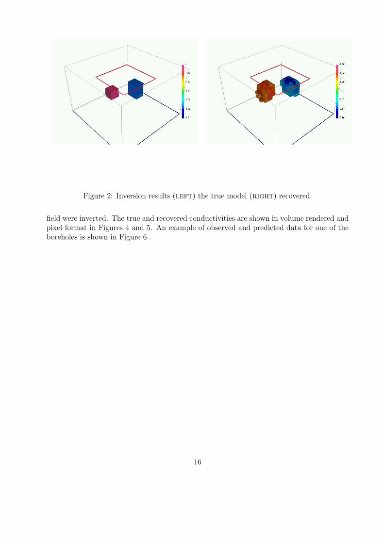
Figure 2: Inversion results (left) the true model (right) recovered.

field were inverted. The true and recovered conductivities are shown in volume rendered andpixel format in Figures 4 and 5. An example of observed and predicted data for one of theboreholes is shown in Figure 6 .

16

Figure 3: The source loop for the UTEM survey is at the surface. Six drill holes are shownin green. Three-component dB/dt data are acquired along the drill holes. The target is theconductive block. Drill hole ]1 just grazes the outside of the target.

17

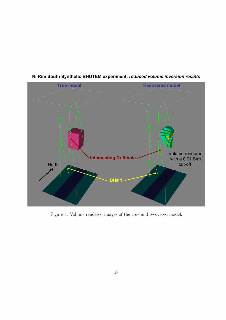
Figure 4: Volume rendered images of the true and recovered model.

18

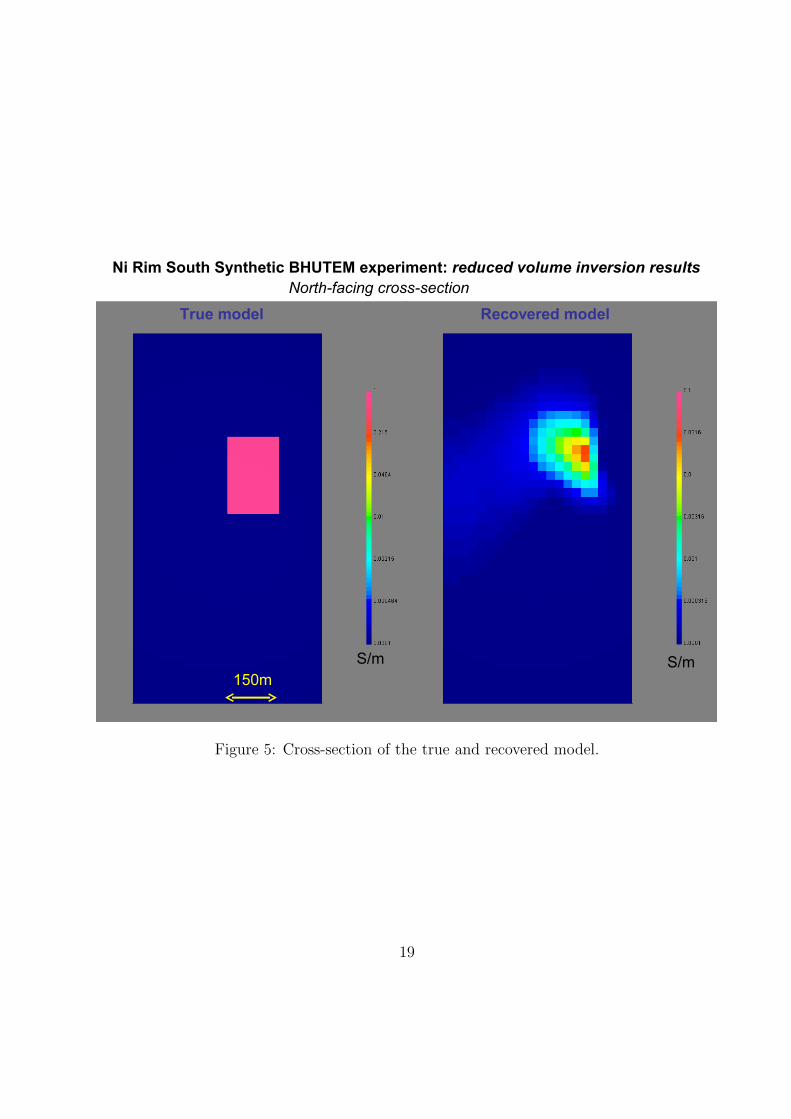
Figure 5: Cross-section of the true and recovered model.

19

Figure 6: Observed and predicted data for the first time channels are plotted along borehole]1.

20

7.3 Working with extended waveforms

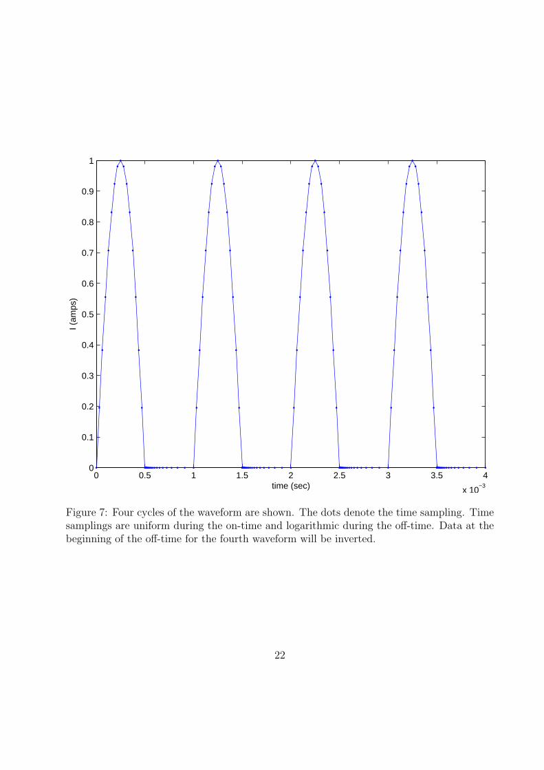
A surface loop survey is carried out over a conductive prism of 8S/m. The waveform isa half-sinusoid followed by an off-time. The frequency of the transmitter is f = 1000Hzand thus the total waveform, comprised of equal length of on-time and off-time segments,is T = .001sec. Because of its high conductivity and size, the time constant for the targetis greater than T . Multiple waveforms are needed and in Figure 7 we plot the first four ofthese along with the time sampling. Constant time-steps were used in the on-time of thewaveform, but logarithmic samples were used in the offtime. The number of time sampleswas 193. Also in Figure 8 we plot the decay curves for Hz for the first four cycles. There isa substantial difference between successive decays.

We next take the fourth decay and use that as data for the inverse problem. All threecomponents of noise-contaminated magnetic field are inverted. The inversion is carried outby setting te to be the time of the first data channel. One processor is used to run theforward modelling from [0, te−1] and stores the field ute−1. This field is updated every timethat the model is changed. The second processor, which is working on generating a modelperturbation, begins each forward modelling with the stored field.

The success of this approach requires that the fields at te from a previous model are closeto the fields that would have been obtained if a complete modelling had been done on thecurrent model. We have compared the misfit obtained by starting with a near-by model, tothat obtained by carrying out a full modelling. We note that the discrepancies between thetwo are reduced as the iterations increase. This is because size of the model perturbationdecreases as the procedure reaches convergence.

An image of the true and constructed models are presented in Figure 9.

21

0 0.5 1 1.5 2 2.5 3 3.5 4

x 10−3

0

0.1

0.2

0.3

0.4

0.5

0.6

0.7

0.8

0.9

1

time (sec)

I (am

ps)

Figure 7: Four cycles of the waveform are shown. The dots denote the time sampling. Timesamplings are uniform during the on-time and logarithmic during the off-time. Data at thebeginning of the off-time for the fourth waveform will be inverted.

22

−5.5 −5 −4.5 −4 −3.5

−4

−3.5

−3

−2.5x 10

−4

log t

Hz

(Am

p/m

)

(1)

−5.5 −5 −4.5 −4 −3.5

−5.5

−5

−4.5

−4

−3.5x 10

−4

log t

Hz

(Am

p/m

)

(2)

−5.5 −5 −4.5 −4 −3.5−6.5

−6

−5.5

−5

−4.5

−4x 10

−4

log t

Hz

(Am

p/m

)

(3)

−5.5 −5 −4.5 −4 −3.5

−6.5

−6

−5.5

−5

−4.5

x 10−4

log t

Hz

(Am

p/m

)

(4)

Figure 8: Response curves for Hz at a station near the center of the loop. Labels (1) - (4)respectively refer to the measurements after the respective number of on-time pulses.

23

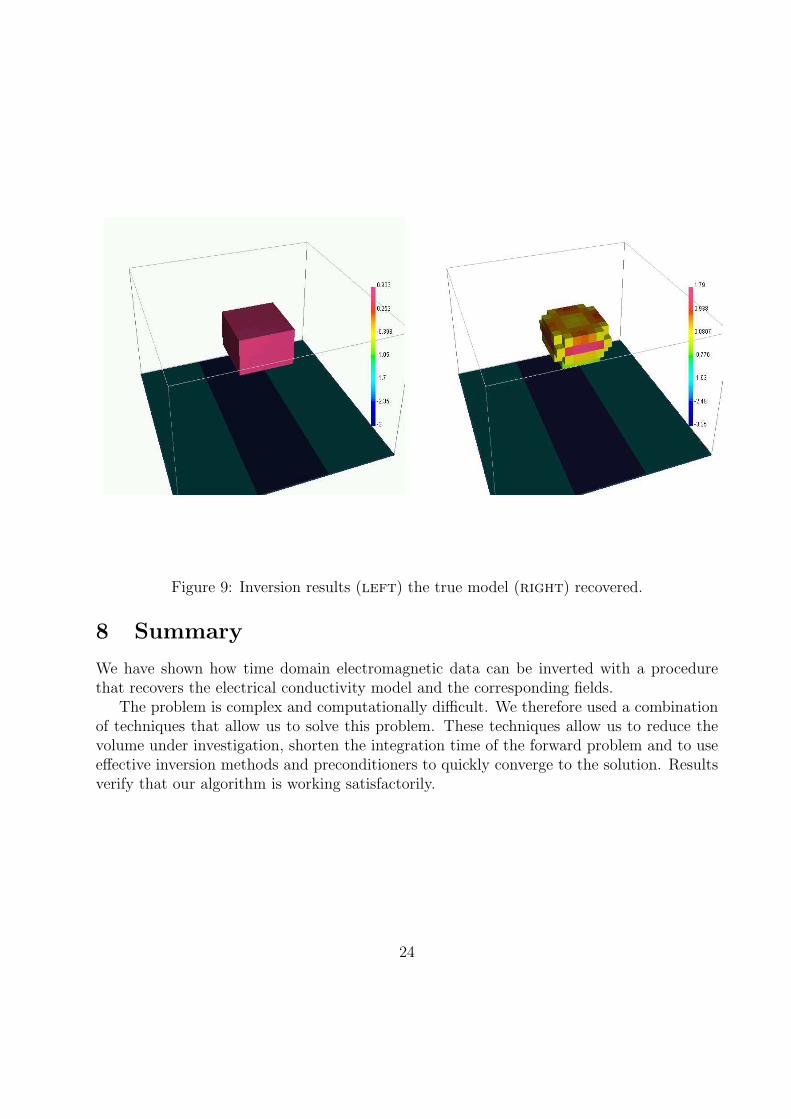
Figure 9: Inversion results (left) the true model (right) recovered.

8 Summary

We have shown how time domain electromagnetic data can be inverted with a procedurethat recovers the electrical conductivity model and the corresponding fields.

The problem is complex and computationally difficult. We therefore used a combinationof techniques that allow us to solve this problem. These techniques allow us to reduce thevolume under investigation, shorten the integration time of the forward problem and to useeffective inversion methods and preconditioners to quickly converge to the solution. Resultsverify that our algorithm is working satisfactorily.

24

9 Appendix:Calculating Derivatives

In order to compute the gradient of the objective function (1.8) we need to evaluate theaction of the sensitivity matrix times a vector. While the matrices A(m) and Q are welldefine we further need to evaluate the matrix G(m,u), where

G(m,u) =∂[A(m)u]

∂m.

The above formula implies that in order to calculate the matrix G(m) we need to differentiatethe forward modeling matrix times a vector with respect to m. This may look complicatedat first; however, note that the matrix A is made of blocks and each block depends on monly through the matrix Mσ. Therefore, if we know how to calculate

N(m, v) =∂[Mσ(m)v]

∂m

then we can differentiate any product involving Mσ. For example,

∂

∂m[∇h · Mσ∇hw] = ∇h · N(m,∇hw).

To calculate this derivative, we recall that Mσ operates on the discrete A or ∇hφ whichare cell face variables. The matrix is diagonal and each of its elements has the form

M(ii)σ = 2(σ−1

1 + σ−12 )−1

where σ1 and σ2 are the values of σ at the two sides of the face of the cell. From this formit is clear that M−1

σ is linear with respect to σ−1 and therefore the matrix

Nr(v) =∂[M−1

σ v]

∂[σ−1]

is independent of σ and depends only on the vector field v at each cell. Using this observationand the chain rule we can easily calculate N ,

N(m, v) =∂[Mσ(m)v]

∂m=

∂[((Mσ(m))−1)

−1v]

∂m=

∂[((Mσ(m))−1)

−1v]

∂[σ−1]

∂[σ−1]

∂m=

[M−1σ ]−2 Nr(v) diag(exp(−m)) = M2

σ Nr(v) diag(exp(−m)).

Given the above gradients we can proceed and discuss the solution of the nonlinear system(1.8).

25

References

[1] D. Aruliah and U. Ascher. Multigrid preconditioning for time-harmonic maxwell’s equa-tions in 3D. Preprint, 2000.

[2] U. Ascher and E. Haber. Grid refinement and scaling for distributed parameter estima-tion problems. Inverse Problems, 17:571–590, 2001.

[3] U. Ascher and E. Haber. A multigrid method for distributed parameter estimationproblems. ETNA, 15:1–15, 2003.

[4] U.M. Ascher and L.R. Petzold. Computer Methods for Ordinary Differential Equationsand Differential-Algebraic Equations. SIAM, Philadelphia, 1998.

[5] G. Biros and O. Ghattas. Parallel Lagrange-Newton-Krylov-Schur methods for PDE-constrained optimization Parts I,II. Preprints, 2000.

[6] L. Borcea, J. G. Berryman, and G. C. Papanicolaou. High-contrast impedance tomog-raphy. Inverse Problems, 12, 1996.

[7] M. Cheney, D. Isaacson, and J.C. Newell. Electrical impedance tomography. SIAMReview, 41:85–101, 1999.

[8] U. Clarenz, M. Droske, and M. Rumpf. Towards fast non–rigid registration. In InverseProblems, Image Analysis and Medical Imaging, AMS Special Session Interaction ofInverse Problems and Image Analysis, volume 313, pages 67–84. AMS, 2002.

[9] J. E. Dennis and R. B. Schnabel. Numerical Methods for Unconstrained Optimizationand Nonlinear Equations. SIAM, Philadelphia, 1996.

[10] A. J. Devaney. The limited-view problem in diffraction tomography. Inverse Problems,5:510–523, 1989.

[11] H.W. Engl, M. Hanke, and A. Neubauer. Regularization of Inverse Problems. Kluwer,1996.

[12] C. Farquharson and D. Oldenburg. Non-linear inversion using general measures of datamisfit and model structure. Geophysics J., 134:213–227, 1998.

[13] Luc Gilles, C.R. Vogel, and J.M. Bardsley. Computational methods for a large-scaleinverse problem arising in atmospheric optics. Inverse Problems, 18:237–252, 2002.

[14] E. Haber. A multilevel, level-set method for optimizing eigenvalues in shape designproblems. JCP, 115:1–15, 2004.

[15] E. Haber. Quasi-newton methods methods for large scale electromagnetic inverse prob-lems. Inverse Peoblems, 21, 2005.

26

[16] E. Haber and U. Ascher. Fast finite volume simulation of 3D electromagnetic problemswith highly discontinuous coefficients. SIAM J. Scient. Comput., 22:1943–1961, 2001.

[17] E. Haber and U. Ascher. Preconditioned all-at-one methods for large, sparse parameterestimation problems. Inverse Problems, 17:1847–1864, 2001.

[18] E. Haber, U. Ascher, D. Aruliah, and D. Oldenburg. Fast simulation of 3D electromag-netic using potentials. J. Comput. Phys., 163:150–171, 2000.

[19] E. Haber, U. Ascher, and D. Oldenburg. Solution of the 3D electromagntic inverseproblem. In Third Int. Symp. on 3D Electromagnetics, Salt Lake City, Oct 1999.

[20] E. Haber, U. Ascher, and D. Oldenburg. On optimization techniques for solving non-linear inverse problems. Inverse problems, 16:1263–1280, 2000.

[21] E. Haber, U. Ascher, and D. Oldenburg. Inversion of frequency and time domainelectromagnetic data. Geophysics, 69:1216–1228, 2004. n5.

[22] E. Haber and D. Oldenburg. A GCV based methods for nonlinear inverse problem.Computational Geoscience, 4, 2000. n1.

[23] E. Haber, D. Oldenburg, and U. Ascher. Modelling 3D maxwell’s equations with non-continuous coefficients. In SEG, Calgary, Aug 2000.

[24] P. J. Huber. Robust estimation of a location parameter. Ann. Math. Stats., 35:73–101,1964.

[25] C.T. Kelley. Iterartive Methods for Optimization. SIAM, Philadelphia, 1999.

[26] J. Nocedal and S. Wright. Numerical Optimization. New York: Springer, 1999.

[27] R. L. Parker. Geophysical Inverse Theory. Princeton University Press, Princeton NJ,1994.

[28] Y. Saad. Iterartive Methods for Sparse Linear Systems. PWS Publishing Company,1996.

[29] N.C. Smith and K. Vozoff. Two dimensional DC resistivity inversion for dipole dipoledata. IEEE Trans. on geoscience and remote sensing, GE 22:21–28, 1984. Special issueon electromagnetic methods in applied geophysics.

[30] C. Vogel. Sparse matrix computation arising in distributed parameter identification.SIAM J. Matrix Anal. Appl., 20:1027–1037, 1999.

[31] G. Wahba. Spline Models for Observational Data. SIAM, Philadelphia, 1990.

[32] S.H. Ward and G.W. Hohmann. Electromagnetic theory for geophysical applications.Electromagnetic Methods in Applied Geophysics, 1:131–311, 1988. Soc. Expl. Geophys.

27