Inverse random source problems for time-harmonic acoustic ...

Full Terms & Conditions of access and use can be found athttps://www.tandfonline.com/action/journalInformation?journalCode=lpde20

Communications in Partial Differential Equations

ISSN: 0360-5302 (Print) 1532-4133 (Online) Journal homepage: https://www.tandfonline.com/loi/lpde20

Inverse random source problems for time-harmonic acoustic and elastic waves

Jianliang Li, Tapio Helin & Peijun Li

To cite this article: Jianliang Li, Tapio Helin & Peijun Li (2020) Inverse random source problemsfor time-harmonic acoustic and elastic waves, Communications in Partial Differential Equations,45:10, 1335-1380, DOI: 10.1080/03605302.2020.1774895

To link to this article: https://doi.org/10.1080/03605302.2020.1774895

Published online: 05 Jun 2020.

Submit your article to this journal

Article views: 49

View related articles

View Crossmark data

https://www.tandfonline.com/action/journalInformation?journalCode=lpde20

https://www.tandfonline.com/loi/lpde20

https://www.tandfonline.com/action/showCitFormats?doi=10.1080/03605302.2020.1774895

https://doi.org/10.1080/03605302.2020.1774895

https://www.tandfonline.com/action/authorSubmission?journalCode=lpde20&show=instructions

https://www.tandfonline.com/action/authorSubmission?journalCode=lpde20&show=instructions

https://www.tandfonline.com/doi/mlt/10.1080/03605302.2020.1774895

https://www.tandfonline.com/doi/mlt/10.1080/03605302.2020.1774895

http://crossmark.crossref.org/dialog/?doi=10.1080/03605302.2020.1774895&domain=pdf&date_stamp=2020-06-05


Inverse random source problems for time-harmonicacoustic and elastic waves

Jianliang Lia, Tapio Helinb, and Peijun Lic

aSchool of Mathematics and Statistics, Changsha University of Science and Technology, Changsha, P.R.China; bSchool of Engineering Science, LUT University, Lappeenranta, Finland; cDepartment ofMathematics, Purdue University, West Lafayette, IN, USA

ABSTRACTThis paper concerns the random source problems for the time-har-monic acoustic and elastic wave equations in two and three dimen-sions. The goal is to determine the compactly supported externalforce from the radiated wave field measured in a domain away fromthe source region. The source is assumed to be a microlocally iso-tropic generalized Gaussian random function such that its covarianceoperator is a classical pseudo-differential operator. Given such a dis-tributional source, the direct problem is shown to have a uniquesolution by using an integral equation approach and the Sobolevembedding theorem. For the inverse problem, we demonstrate thatthe amplitude of the scattering field averaged over the frequencyband, obtained from a single realization of the random source, deter-mines uniquely the principle symbol of the covariance operator. Theanalysis employs asymptotic expansions of the Green functions andmicrolocal analysis of the Fourier integral operators associated withthe Helmholtz and Navier equations.

ARTICLE HISTORYReceived 12 October 2018Accepted 15 May 2020

KEYWORDSElastic wave equation;Gaussian random function;Helmholtz equation; inversesource problem; uniqueness

2010 MATHEMATICSSUBJECTCLASSIFICATION78A46; 65C30

1. Introduction

The inverse source scattering in waves, as an important and active research subject ininverse scattering theory, are to determine the unknown sources that generate pre-scribed radiated wave patterns [1]. It has been considered as a basic mathematical toolfor the solution of many medical imaging modalities [2], such as magnetoencephalogra-phy (MEG), electroencephalography (EEG), and electroneurography (ENG). Theseimaging modalities are noninvasive neurophysiological techniques that measure the elec-tric or magnetic fields generated by neuronal activity of the brain. The spatial distribu-tions of the measured fields are analyzed to localize the sources of the activity withinthe brain to provide information about both the structure and function of the brain[3–5]. The inverse source scattering problem has also attracted much research in thecommunity of antenna design and synthesis [6]. A variety of antenna-embedding mate-rials or substrates, including non-magnetic dielectrics, magneto-dielectrics, and doublenegative meta-materials are of great interest.

CONTACT Peijun Li [email protected] Department of Mathematics, Purdue University, West Lafayette,IN 47907-2050, USA.� 2020 Taylor & Francis Group, LLC

COMMUNICATIONS IN PARTIAL DIFFERENTIAL EQUATIONS2020, VOL. 45, NO. 10, 1335–1380https://doi.org/10.1080/03605302.2020.1774895


http://www.tandfonline.com

Driven by these significant applications, the inverse source scattering problems havecontinuously received much attention and have been extensively studied by manyresearchers. There are a lot of available mathematical and numerical results, especiallyfor the acoustic waves or the Helmholtz equation [7–12]. In general, the inverse sourceproblem does not have a unique solution due to the existence of non-radiating sources[13–15]. Some additional constraint or information is needed in order to obtain aunique solution, such as to seek the minimum energy solution which represents thepseudo-inverse solution for the inverse problem. For electromagnetic waves, Ammariet al. showed uniqueness and presented an inversion scheme in [3] to reconstruct dipolesources based on a low-frequency asymptotic analysis of the time-harmonic Maxwellequations. In [16], Albanese and Monk discussed uniqueness and non-uniqueness of theinverse source problems for Maxwell’s equations. Computationally, a more serious issueis the lack of stability, i.e., a small variation in the measured data may lead to a hugeerror in the reconstruction. Recently, it has been realized that the use of multi-fre-quency data can overcome the difficulties of non-uniqueness and instability which areencountered at a single frequency. In [17], Bao et al. initialized the mathematical studyon the stability of the inverse source problem for the Helmholtz equation by usingmulti-frequency data. Since then, the increasing stability has become an interestingresearch topic in the study of inverse source problems [18–20]. We refer to [21] for atopic review on solving general inverse scattering problems with multi-frequencies.Recently, the elastic wave scattering problems have received ever increasing attention

for their important applications in many scientific areas such as geophysics and seismol-ogy [22–26]. However, the inverse source problem is much less studied for the elasticwaves. The elastic wave equation is challenging due to the coexistence of compressionaland shear waves that have different wavenumbers. Consequently, the Green tensor ofthe Navier equation has a more complicated expression than the Green function of theHelmholtz equation does. A more sophisticated analysis is required.In many applications the source and hence the radiating field may inherently be con-

sidered random [27]. Therefore, their governing equations are stochastic differentialequations. Although the deterministic counterparts have been well studied, little isknown for the stochastic inverse problems due to randomness and uncertainties. Auniqueness result may be found in [28] for an inverse random source problem. It wasshown that the auto-correlation function of the random source was uniquely deter-mined by the auto-correlation function of the radiated field. Recently, effective mathem-atical models and efficient computational methods have been developed in [29–34] forinverse random source scattering problems, where the stochastic wave equations areconsidered and the random sources are assumed to be driven by additive white noise.In stochastic setting the inverse problems are often formulated to determine the statis-tical properties such as the mean and variance. The methods mentioned are based onobservations of the correlations in the scattering data. By the strong law of large num-bers, the correlations have to be approximated by taking fairly large number of realiza-tions of the measurement. We refer to [35] for statistical inversion theory on generalrandom inverse problems.This paper takes another perspective to randomness following earlier work in

[36–38]. We assume that all the data is produced by a single realization of a random

1336 J. LI ET AL.

source. If the data is exceptional noisy or corrupted, the recovery of this single sourcerealization may be infeasible. However, it may be possible to recover some statisticalparameters of the source if observations of the radiating field are available at multiplewavelengths.Here, we develop a unified theory on both of the direct and inverse scattering prob-

lems for the time-harmonic acoustic and elastic wave equations. The source is assumedto be a generalized Gaussian random function which is supported in a bounded domain

D � Rd, d¼ 2 or 3. In addition, we assume that the covariance of the random source is

described by a pseudo-differential operator with the principle symbol given by

/ðxÞjnj�m, m 2�d, d þ 1

2

�,

where / is a smooth non-negative function supported on D and is called the micro-cor-relation strength of the source. The parameter m indicates how irregular realizationssuch a random process has. What is more, the micro-correlation strength identifieswhere this most irregular behavior is strongest and where it is more dampened. Thislarge class of random fields includes stochastic processes like the fractional Brownianmotion and Markov field [38].When m 2 ½d, d þ 1

2Þ, we can only ensure that the source belongs to a Sobolev spacewith negative smoothness index almost surely. Hence, the direct scattering problemrequires a careful analysis since the source is non-smooth. In this work, we establish thewell-posedness of the direct scattering problems for both wave equations with suchrough sources in Theorems 3.3 and 4.3, respectively.The inverse scattering problem aims at reconstructing the micro-correlation strength

of the source / from the scattered field measured in a bounded domain U where �U \�D ¼ ;: For a single realization of the random source, we measure the amplitude of thescattering field averaged over the frequency band in a bounded and simply connecteddomain U, i.e., for some large Q> 0, our data is given byðQ

1jsjuðx, jÞj2dj or

ðQ1xsjuðx,xÞj2dx, x 2 U , (1.1)

where s 2 Rþ depends on m, j > 0 and x > 0 are the wavenumber and the angular

frequency, u and u represents the pressure of the acoustic wave equation and the dis-placement of the elastic wave equation, respectively.Combining harmonic and microlocal analysis, we show that: for acoustic waves, the

micro-correlation strength function / can be recovered given data in (1.1); For elasticwaves, note that the source is a vector, if the components of the random source areindependent and the principle symbol of the pseudo-differential operator of each com-ponent coincides, thus, the micro-correlation strength function / can be determineduniquely by these measurements.This work is motivated by [36, 38], where an inverse problem was considered for the

two-dimensional random Schr€odinger equation. The potential function in theSchr€odinger equation was assumed to be a Gaussian random function with a pseudo-differential operator describing its covariance. It was shown that the principle symbol ofthe covariance operator can be determined uniquely by the backscattered field,

COMMUNICATIONS IN PARTIAL DIFFERENTIAL EQUATIONS 1337

generated by a single realization of the random potential and a point source as the inci-dent field. A closely related problem can be found in [37]. The authors considered theuniqueness for an inverse acoustic scattering problem in a half-space with an impedanceboundary condition, where the impedance coefficient was assumed to be a Gaussianrandom function whose covariance operator is a pseudo-differential operator.The paper is organized as follows. In Section 2, we introduce some commonly used

Sobolev spaces, give a precise mathematical description of the generalized Gaussian ran-dom function, and present several lemmas on rough fields and random variables.Section 3 is devoted to the study of the acoustic wave equation in the two- and three-dimensional cases. The well-posedness of the direct problems are examined. Theuniqueness of the inverse problem is achieved. Section 4 addresses the two- and three-dimensional elastic wave equations. Analogous results are obtained. The direct problemis shown to have a unique solution and the inverse problem is proved to have theuniqueness to recover the principle symbol of the covariance operator for the randomsource. This paper is concluded with some general remarks in Section 5.

2. Preliminaries

In this section, we introduce some necessary notation such as Sobolev spaces and gener-alized Gaussian random functions which are used throughout the paper.

2.1. Sobolev spaces

Let Rd be the d-dimensional space, where d ¼ 2 or 3: Denote by C1

0 ðRdÞ the set of

smooth functions with compact support and by D0ðRdÞ the set of generalized (distribu-

tional) functions. For 1 < p < 1, s 2 R, the Sobolev space Hs, pðRdÞ is defined by

Hs, pðRdÞ ¼ fh ¼ ðI � DÞ�s2g : g 2 LpðRdÞg,

which has the norm

jjhjjHs, pðRdÞ ¼ jjðI � DÞs2hjjLpðRdÞ:

With the definition of Sobolev spaces in the whole space, we can define the Sobolev

spaces Hs, pðVÞ for any Lipschitz domain V � Rd as the restrictions to V of the ele-

ments in Hs, pðRdÞ: The norm is defined by

jjhjjHs, pðVÞ ¼ inffjjgjjHs, pðRdÞ : gjV ¼ hg:

According to [39], for s 2 R and 1 < p < 1, we can define Hs, p0 ðVÞ as the space of all

distributions h 2 Hs, pðRdÞ such that supph � �V and the the norm is defined by

jjhjjHs, p0 ðVÞ ¼ jjhjjHs, pðRdÞ:

It is known that C10 ðVÞ is dense in Hs, p

0 ðVÞ for any 1 < p < 1, s 2 R; C10 ðVÞ is dense

in Hs, pðVÞ for any 1 < p < 1, s � 0; C1ð�V Þ is dense in Hs, pðVÞ for any 1 < p < 1,s 2 R: Additionally, by [39, Propositions 2.4 and 2.9], for any s 2 R, p, q 2 ð1,1Þsatisfying 1

p þ 1q ¼ 1, we have

1338 J. LI ET AL.

H�s, q0 ðVÞ ¼ ðHs, pðVÞÞ0 and H�s, qðVÞ ¼ ðHs, p

0 ðVÞÞ0,where the prime denotes the dual space.

2.2. Generalized gaussian random functions

In this subsection, we provide a precise mathematical description of the generalizedGaussian random function. Let ðX,F ,PÞ be a complete probability space. The function

q is said to be a generalized Gaussian random function if q : X ! D0ðRdÞ is a measur-able map such that for every x̂ 2 X, the mapping x̂ 2 X 7! hqðx̂Þ,wi is a Gaussian

random variable for all w 2 C10 ðRdÞ: The expectation and the covariance of the general-

ized Gaussian random function q can be defined by

Eq : w 2 C10 ðRdÞ 7!Ehq,wi 2 R,

Covq : ðw1,w2Þ 2 C10 ðRdÞ2 7!Covðhq,w1i, hq,w2iÞ 2 R,

where Ehq,wi denotes the expectation of hq,wi andCovðhq,w1i, hq,w2iÞ ¼ Eððhq,w1i � Ehq,w1iÞðhq,w2i � Ehq,w2iÞÞ

denotes the covariance of hq,w1i and hq,w2i: The covariance operator Cq : C10 ðRdÞ !

D0ðRdÞ is defined by

hCqw1,w2i ¼ Covðhq,w1i, hq,w2iÞ ¼ Eðhq� Eq,w1ihq� Eq,w2iÞ: (2.1)

Let kqðx, yÞ be the Schwartz kernel of the covariance operator Cq. We also call kqðx, yÞthe covariance function of q. Thus, (2.1) means that

kqðx, yÞ ¼ EððqðxÞ � EqðxÞÞðqðyÞ � EqðyÞÞÞ (2.2)

in the sense of generalized functions.In this paper, we assume that each component of the external source is a generalized,

microlocally isotropic Gaussian random function. For this end, let D � Rd be a

bounded and simply connected domain. We introduce the following definition.

Definition 2.1. A generalized Gaussian random function q on Rd is called microlocally

isotropic of order m in D, if the realizations of q are almost surely supported in thedomain D and its covariance operator Cq is a classical pseudo-differential operator

having the principal symbol /ðxÞjnj�m, where / 2 C10 ðRdÞ, supp/ � D and /ðxÞ � 0

for all x 2 Rd:

We refer to [36, 38] for examples, such as fractional Brownian motion and Markovfield, and numerical illustrations of random fields and covariance structures, whichsatisfy the above definition. Recall that the parameter m indirectly indicates theSobolev smoothness of the realizations of the field as we will see in the next lemmaand the microlocal strength identifies the amplitude of these oscillations. In particular,we are interested in the case m 2 ½d, d þ 1

2Þ, which corresponds to rough fields. Nowwe introduce three lemmas and give an assumption which will be used in subse-quent analysis.


Lemma 2.2. Let f be a generalized and microlocally isotropic Gaussian random functionof order m in D. If m¼ d, then f 2 H�e, pðDÞ almost surely for all e > 0, 1 < p < 1. If

m 2 d, d þ 12

� �, then f 2 CaðDÞ almost surely for all a 2 0, m�d

2

� �:

Lemma 2.3. Let X and Y be two zero-mean random variables such that the pair (X, Y) isa Gaussian random vector. Then we have

EððX2 � EX2ÞðY2 � EY2ÞÞ ¼ 2ðEXYÞ2:

Lemma 2.4. Let Xt, t � 0 be a real valued stochastic process with a continuous path ofzero mean, i.e., EXt ¼ 0. Assume that for some constants c> 0 and b > 0 such that thecondition

jEðXtXtþrÞj � cð1þ rÞ�b (2.3)

holds for all t, r � 0. Then

limQ!1

1Q

ðQ1Xtdt ¼ 0

almost surely.

Lemma 2.2 is a direct consequence of Theorem 2 in [38]. Lemma 2.3 is shown in[36] as Lemma 4.2. The ergodic result of Lemma 2.4 is an immediate corollary of [40,p. 94]. To establish the main results, we need the following assumption.

Assumption A. The external source f is assumed to have a compact support D � Rd:

Let U � Rd n �D be the measurement domain of the wave field. We assume that D and

U are two bounded and simply connected domains and there is a positive distancebetween D and U.

3. Acoustic waves

This section addresses the direct and inverse source scattering problems for theHelmholtz equation in two- and three-dimensional space. The external source isassumed to be a generalized Gaussian random function whose covariance operator is aclassical pseudo-differential operator. The direct problem is shown to have a uniquesolution. For the inverse problem, we show that the principle symbol of the covarianceoperator can be determined uniquely by the scattered field obtained from a single real-ization of the random source.

3.1. The direct scattering problem

Consider the Helmholtz equation in a homogeneous medium

Duþ j2u ¼ f in Rd, (3.1)

where j > 0 is the wavenumber, u is the wave field, and f is a generalized Gaussian ran-dom function. Note that u is a random field since f is a random function. To ensure

1340 J. LI ET AL.

the uniqueness of the solution for (3.1), the usual Sommerfeld radiation condition isimposed

limr!1 r

d�12 @ru� ijuð Þ ¼ 0, r ¼ jxj, (3.2)

uniformly for all directions x̂ ¼ x=jxj: In addition, the external source function f satis-fies the following assumption.

Assumption B. The generalized Gaussian random field f is microlocally isotropic oforder m in D, where m 2 ½d, d þ 1

2Þ: The principle symbol of its covariance operator Cf

is /ðxÞjnj�m with / 2 C10 ðDÞ and / � 0: Moreover, the mean value of f is zero,

i.e., Eðf Þ ¼ 0:Recall that by Lemma 2.2, the random source f ðx̂Þ belongs with probability one to

the Sobolev space H�e, pðDÞ for all e > 0, 1 < p < 1: Hence it suffices to show that thedirect scattering problem is well-posed when f is a deterministic non-smooth functionin H�e, pðDÞ:First, we show some regularity results of the fundamental solution. These results play

an important role in the proof of the well-posedness. Let Udðx, y, jÞ be the fundamentalsolution for the two- and three-dimensional Helmholtz equation. Explicitly, we have

U2ðx, y, jÞ ¼ i4Hð1Þ

0 ðjjx � yjÞ, U3ðx, y, jÞ ¼ 14p

eijjx�yj

jx� yj , (3.3)

where Hð1Þ0 is the Hankel function of the first kind with order zero. We shall study the

asymptotic properties of the fundamental solutions and their derivatives when x is closeto y. For the two-dimensional case, we recall that

Hð1Þn ðtÞ ¼ JnðtÞ þ iYnðtÞ, (3.4)

where Jn and Yn are the Bessel functions of the first and second kind with order n,respectively. They admit the following expansions

JnðtÞ ¼X1p¼0

ð�1Þpp!ðnþ pÞ!

t2

� �nþ2p

,

YnðtÞ ¼ 2p

lnt2þ c

JnðtÞ � 1

p

Xn�1

p¼0

ðn� 1� pÞ!p!

2t

� �n�2p

� 1p

X1p¼0

ð�1Þpp!ðnþ pÞ!

t2

� �nþ2p

fwðpþ nÞ þ wðpÞg,

(3.5)

where c :¼ limp!1Pp

j¼1 j�1 � ln p

n odenotes the Euler constant, wð0Þ ¼ 0, wðpÞ ¼Pp

j¼1 j�1, and the finite sum in (3.5) is set to be zero for n¼ 0. Using (3.4)–(3.5), we

may verify that

Hð1Þ0 ðtÞ ¼ 2i

pln

t2þ 1þ 2i

pc

� �þ O t2 ln

t2

� �, (3.6)


Hð1Þ1 ðtÞ ¼ � 2i

p1tþ ipt ln

t2þ 1þ 2i

pc� i

p

� �t2þ O t3 ln

t2

� �: (3.7)

Using the recurrence relations for the Hankel function of the first kind (see [41, Eq.(5.6.3)])

ddt

t�nHð1Þn ðtÞ

h i¼ �t�nHð1Þ

nþ1ðtÞ, (3.8)

we may show from (3.6) to (3.7) that


0 ðjjx� yjÞ

¼ � 12p

lnjx � yj

2þ i

4� c2p

� �þ O jx � yj2 ln jx � yj

2

� �,

(3.9)

@yiU2ðx, y, jÞ ¼ �ji4ðyi � xiÞH

ð1Þ1 ðjjx� yjÞjx � yj

¼ � 12p

yi � xijx � yj2 þ Oððyi � xiÞ ln jx � yj

2Þ:

(3.10)

For the three-dimensional case, a simple calculation yields that

U3ðx, y, jÞ ¼ eijjx�yj

4pjx � yj , (3.11)

@yiU3ðx, y, jÞ ¼ ðyi � xiÞ4pjx � yj3 e

ijjx�yjðijjx� yj � 1Þ: (3.12)

Lemma 3.1. Given any x 2 Rd, we have U2ðx, � , jÞ 2 L2locðR2Þ \ H1, p

loc ðR2Þ for any p 2ð1, 2Þ and U3ðx, � , jÞ 2 L2locðR3Þ \H1, p

loc ðR3Þ for any p 2 1, 32� �

:

Proof. For any fixed x 2 Rd, let V � R

d be a bounded domain containing x. Denote q :¼supy2V jx � yj, then we have V � BqðxÞ:For d¼ 2, by (3.9) and (3.10), it suffices to show that

lnjx� yj

22 L2ðVÞ, yi � xi

jx � yj2 2 LpðVÞ, 8 p 2 ð1, 2Þ:

A direct calculation yieldsðV

�� ln jx� yj2

��2

dy �ðBqðxÞ

�� ln jx� yj2

��2

dy�ðq0r

�� ln r2

��2

dr < 1

and ðV

�� yi � xijx� yj2

��p

dy �ðBqðxÞ

1

jx� yjp dy�ðq0r1�pdr < 1, 8 p 2 ð1, 2Þ:

1342 J. LI ET AL.

Hereafter, the notation a� b means a � Cb, where C> 0 is a generic constant which

may change step by step in the proofs. Thus, we conclude that U2ðx, � , jÞ 2 L2locðR2Þ \H1, p

loc ðR2Þ for any p 2 ð1, 2Þ:For d¼ 3, from (3.11) and (3.12), it suffices to prove that

eijjx�yj

jx� yj 2 L2ðVÞ, eijjx�yj yi � xijx � yj3 2 LpðVÞ 8 p 2 1,

32

� �:

Similarly, we may have from a simple calculation thatðV

�� eijjx�yj

jx� yj��2

dy �ðBqðxÞ

1

jx � yj2 dy�ðq01dr < 1

and ðV

��eijjx�yj yi � xijx � yj3

��p

dy �ðBqðxÞ

1

jx � yj2p dy�ðq0r2�2pdr < 1 8 p 2 1,

32

� �,

which show that U3ðx, � , jÞ 2 L2locðR3Þ \H1, ploc ðR3Þ for any p 2 1, 32

� �: w

Let V and G be any two bounded domains in Rd: By Lemma 3.1 and the Sobolev

embedding theorem, we obtain that Udðx, � , jÞ 2 HsðVÞ where s 2 ð0, 1Þ for d¼ 2 ands 2 0, 12� �

for d¼ 3. Hence, given g 2 H�s0 ðVÞ, we can define the operator Hj in the

dual sense by

HjgðxÞ ¼ðVUdðx, y, jÞgðyÞdy, x 2 G:

Following the similar arguments in [42, Theorem 8.2], we may show the followingregularity of the operator Hj: The proof is omitted here for brevity.

Lemma 3.2. The operator Hj : H�s0 ðVÞ ! HsðGÞ is bounded for s 2 ð0, 1Þ in two dimen-

sions or for s 2 0, 12� �

in three dimensions.

Theorem 3.3. For some fixed s 2 0, 1� d6

� �and ~p 2 1, d

d�1

� �, assume 0 < e < s, 1 <

p < minð ~pddþ~pðe�1Þ ,

2ddþ2ðe�sÞÞ and 1

p þ 1p0 ¼ 1, then the scattering problem (3.1)–(3.2) with

the source f 2 H�e, p00 ðDÞ attains a unique solution u 2 He, p

loc ðRdÞ, which can be repre-sented by

uðx, jÞ ¼ �ðDUdðx, y, jÞf ðyÞdy: (3.13)

Proof. It is clear that the scattering problem (3.1)–(3.2) with f¼ 0 only has the zero

solution. Hence the uniqueness follows. Now we focus on the existence. Noting s 20, 1� d

6

� �, we have from a simple calculation that 1 < 2d

dþ2ð1�sÞ <32 : Since 1 < p <

~pddþ~pðe�1Þ , a direct computation shows that 1~p � 1

d <1p � e

d : By Lemma 3.1 and the

Sobolev embedding theorem, we obtain that Udðx, � , jÞ 2 H1, ~ploc ðRdÞ � He, p

loc ðRdÞ: Since


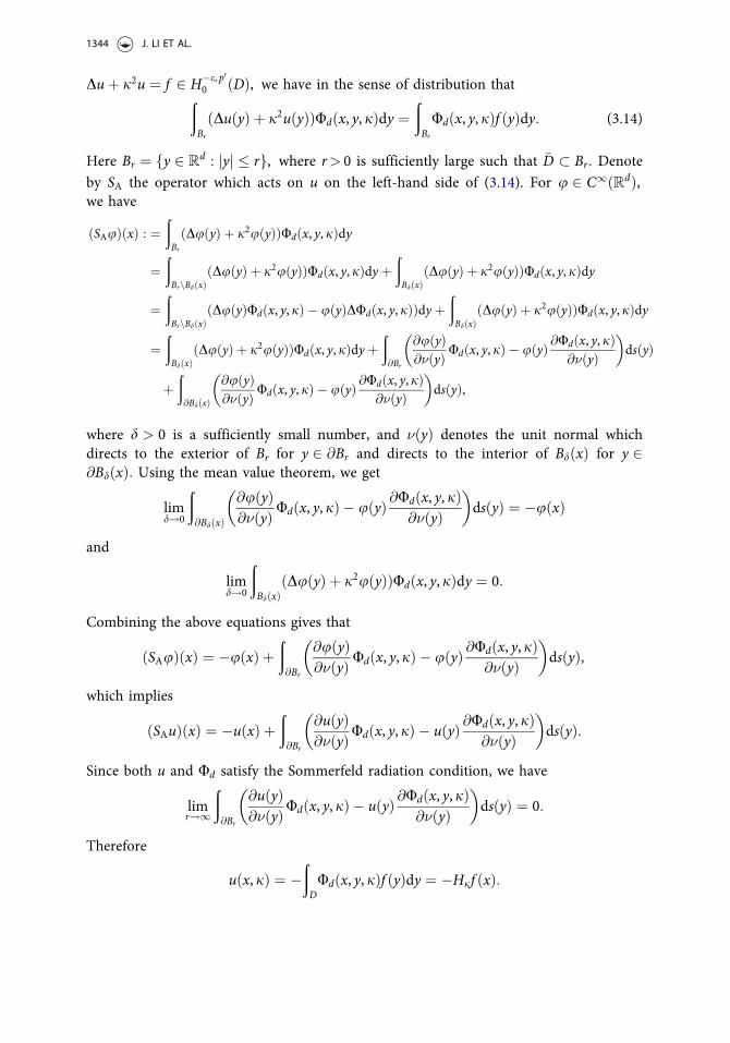
Duþ j2u ¼ f 2 H�e, p00 ðDÞ, we have in the sense of distribution thatðBr

ðDuðyÞ þ j2uðyÞÞUdðx, y, jÞdy ¼ðBr

Udðx, y, jÞf ðyÞdy: (3.14)

Here Br ¼ fy 2 Rd : jyj � rg, where r> 0 is sufficiently large such that �D � Br: Denote

by SA the operator which acts on u on the left-hand side of (3.14). For u 2 C1ðRdÞ,we have

ðSAuÞðxÞ : ¼ðBr

ðDuðyÞ þ j2uðyÞÞUdðx, y, jÞdy

¼ðBrnBdðxÞ

ðDuðyÞ þ j2uðyÞÞUdðx, y, jÞdyþðBdðxÞ

ðDuðyÞ þ j2uðyÞÞUdðx, y, jÞdy

¼ðBrnBdðxÞ

ðDuðyÞUdðx, y, jÞ � uðyÞDUdðx, y,jÞÞdyþðBdðxÞ

ðDuðyÞ þ j2uðyÞÞUdðx, y,jÞdy

¼ðBdðxÞ

ðDuðyÞ þ j2uðyÞÞUdðx, y, jÞdyþð@Br

@uðyÞ@�ðyÞ Udðx, y, jÞ � uðyÞ @Udðx, y, jÞ

@�ðyÞ� �

dsðyÞ

þð@BdðxÞ

@uðyÞ@�ðyÞ Udðx, y, jÞ � uðyÞ @Udðx, y,jÞ

@�ðyÞ� �

dsðyÞ,

where d > 0 is a sufficiently small number, and �ðyÞ denotes the unit normal whichdirects to the exterior of Br for y 2 @Br and directs to the interior of BdðxÞ for y 2@BdðxÞ: Using the mean value theorem, we get

limd!0

ð@BdðxÞ


@�ðyÞ� �

dsðyÞ ¼ �uðxÞ

and

limd!0

ðBdðxÞ

ðDuðyÞ þ j2uðyÞÞUdðx, y, jÞdy ¼ 0:

Combining the above equations gives that

ðSAuÞðxÞ ¼ �uðxÞ þð@Br


@�ðyÞ� �

dsðyÞ,

which implies

ðSAuÞðxÞ ¼ �uðxÞ þð@Br

@uðyÞ@�ðyÞUdðx, y, jÞ � uðyÞ @Udðx, y, jÞ

@�ðyÞ� �

dsðyÞ:

Since both u and Ud satisfy the Sommerfeld radiation condition, we have

limr!1

ð@Br

@uðyÞ@�ðyÞUdðx, y, jÞ � uðyÞ @Udðx, y, jÞ

@�ðyÞ� �

dsðyÞ ¼ 0:

Therefore

uðx, jÞ ¼ �ðDUdðx, y, jÞf ðyÞdy ¼ �Hjf ðxÞ:

1344 J. LI ET AL.

Next is to show that u 2 He, ploc ðRdÞ: From Lemma 3.2, we have that the operator Hj :

H�s0 ðDÞ ! Hs

locðRdÞ for s 2 0, 1� d6

� �is bounded. The assumption 1 < p < 2d

dþ2ðe�sÞimplies that 1

2 þ e�sd < 1

p < 1 which yields 12 � s

d <1p � e

d : Thus, since 0 < e < s, the

Sobolev embedding theorem implies that HsðDÞ is embedded into He, pðDÞ and

H�e, p00 ðDÞ is embedded into H�s

0 ðDÞ: Thus, the operator Hj : H�e, p00 ðDÞ ! He, p

loc ðRdÞ isbounded, which completes the proof. w

3.2. Asymptotics of the correlation data

The three technical results proven in this section lay out the foundations for the proofsof our main results. Notice carefully that the main results for the cases d¼ 2 and d¼ 3will require separate proofs. However, here we formulate general auxiliary lemmas thatmake the deviations of the main proofs moderate. First, in Lemmas 3.4 and 3.5 westudy the general behavior of the asymptotics of the correlation data. At the end of thesection, we prove Lemma 3.6, which will be used in the recovery of the localstrength /:Recall that our strategy is to utilize the ergodicity of the weighted solution process

uðx, jÞ averaged in (1.1) with respect to j and to apply Lemma 2.4. To do this, we needto show that condition (2.3) is satisfied and, therefore, we study the asymptotic correla-tions in uðx, jÞ:To build the general theory, we study the asymptotics of integral

Iðx, j1, j2Þ :¼ 1

jl11 jl22

ðR

2deiðc1j1jx�yj�c2j2jx�zjÞKðx, y, zÞEðqðyÞqðzÞÞdydz (3.15)

where

Kðx, y, zÞ :¼ ðx1 � y1Þm1 � � � ðxd � ydÞmdðx1 � z1Þn1 � � � ðxd � zdÞndjx � yjp1 jx� zjp2 :

Here q stands for a generalized Gaussian random function satisfying Assumption B, andl1, l2, c1, c2, m1,… , nd, p1, p2 are nonnegative constants. Similarly, we define the integral

~Iðx, j1, j2Þ :¼ 1

jl11 jl22

ðR

2deiðc1j1jx�yjþc2j2jx�zjÞKðx, y, zÞEðqðyÞqðzÞÞdydz: (3.16)

Below, in the two next sections we show that the integrals Iðx, j1, j2Þ and ~Iðx, j1, j2Þapproximate the correlation data Eðuðx, j1Þuðx, j2ÞÞ and Eðuðx, j1Þuðx, j2ÞÞ, respect-ively. In fact, in the three-dimensional case, these quantities coincide.

Lemma 3.4. For j1, j2 � 1, the estimates

jIðx, j1, j2Þj � cnðj1 þ j2Þ�ðmþ2minðl1, l2ÞÞð1þ jj1 � j2jÞ�n, (3.17)

jEð~uðx, j1Þ~uðx, j2ÞÞj � cnðj1 þ j2Þ�nð1þ jj1 � j2jÞ�m (3.18)

holds uniformly for x 2 U, where n 2 N is arbitrary.


Proof. To estimate the integral Iðx, j1, j2Þ, we introduce the multiple coordinate trans-formation that allows to use the microlocal methods in our analysis. Noting Eq ¼ 0 and(2.2), we conclude that the correlation function EðqðyÞqðzÞÞ is the Schwartz kernel of a

pseudo-differential operator Cq with a classical symbol rðy, nÞ 2 S�m1, 0 ðRd � R

dÞ which isdefined by

S�m1, 0 ðRd � R

dÞ :¼ faðx, nÞ 2 C1ðRd � RdÞ : j@a

n@bx aðx, nÞj � Ca,bð1þ jnjÞ�m�jajg:

Here a, b are multiple indices, jaj denotes the sum of its component. The principlesymbol of Cq is rpðy, nÞ ¼ /ðyÞjnj�m: The support of EðqðyÞqðzÞÞ is contained inD�D. We can write EðqðyÞqðzÞÞ in terms of its symbol by

EðqðyÞqðzÞÞ ¼ ð2pÞ�dðR

deiðy�zÞ�nrðy, nÞdn: (3.19)

To establish a uniform estimate with respect to the variable x, we extend the covariance

function into the space R2d � R

d, and define B1ðy, z, xÞ ¼ EðqðyÞqðzÞÞhðxÞ where

hðxÞ 2 C10 ðRdÞ equals to one in the domain U and has its support outside of the

domain �D: Thus, we have

B1ðy, z, xÞ ¼ ð2pÞ�dðR

deiðy�zÞ�nc1ðy, x, nÞdn,

where c1ðy, x, nÞ ¼ rðy, nÞhðxÞ 2 S�m1, 0 ðR2d � R

dÞ with a principle symbol

cp1ðy, x, nÞ ¼ /ðyÞjnj�mhðxÞ:To proceed the analysis, let us briefly revisit the conormal distributions of H€ormander

type [43]. If X � Rd is an open set and S � X is a smooth submanifold of X, we denote

by IðX; SÞ the distributions in D0ðXÞ that are smooth in X n S and have a conormal sin-gularity at S. In consequence, by (3.19), the correlation function EðqðyÞqðzÞÞ is a conor-

mal distribution in R2d of H€ormander type having conormal singularity on the surface

S1 ¼ fðy, zÞ 2 R2d : y� z ¼ 0g: Moreover, let IcompðX; SÞ be the set of distributions sup-

ported in a compact subset of X. Let X1 � R3d be an open set containing D� D�

suppðhÞ so that B1 2 IcompðX1; S1 \ X1Þ:Define the first coordinate transformation g : R3d ! R

3d by

ðv,w, xÞ ¼ gðy, z, xÞ ¼ ðy� z, yþ z, xÞ: (3.20)

Substituting the coordinate transformation (3.20) into B1ðy, z, xÞ gives

B2ðv,w, xÞ ¼ B1ðg�1ðv,w, xÞÞ ¼ ð2pÞ�dðR

deiv�nc1

vþ w2

, x, n

� �dn,

which means that B2 2 IðR3d, S2Þ where S2 :¼ fðv,w, xÞ : v ¼ 0g: Actually, B2 2IcompðX2,X2 \ S2Þ where X2 :¼ gðDÞ: To find out how the symbol transforms in thechange of coordinates, we need to represent c1 vþw

2 , x, n� �

with a symbol that does notdepend on v. Using the representation theorem of conormal distribution [43, Lemma18.2.1]), we obtain

1346 J. LI ET AL.

B2ðv,w, xÞ ¼ ð2pÞ�dðR

deiv�nc2ðw, x, nÞdn,

where c2ðw, x, nÞ has the asymptotic expansion

c2ðw, x, nÞ �X1l¼0

h�iDv ,Dnill!

c1vþ w2

, x, n

� ��v¼0

2 S�m1, 0 ðR2d � R

dÞ,

where D is defined by Dj :¼ �i@j: In particular, the principle symbol of c2ðw, x, nÞ is

cp2ðw, x, nÞ ¼ /vþ w2

� �jnj�mhðxÞ

��v¼0

:

We consider the phase of Iðx, j1, j2Þ: A simple calculation shows that

c1j1jx� yj � c2j2jx� zj ¼ ðc1j1 þ c2j2Þ jx� yj � jx� zj2

þ ðc1j1 � c2j2Þ jx � yj þ jx � zj2

:

(3.21)

In the second set of coordinates, let jx�yj6jx�zj2 play the role of two coordinates. We will

do this change in two steps. First, for the two-dimensional case where d¼ 2, we define

s1 : R6 ! R

6 by

s1ðy, z, xÞ ¼ ðE1,E2, xÞ,where E1 ¼ ðt1, s1Þ and E2 ¼ ðt2, s2Þ with

t1 ¼ 12jx� yj, s1 ¼ 1

2jx � yjarcsin y1 � x1

jx� yj� �

,

t2 ¼ 12jx� zj, s2 ¼ 1

2jx� zjarcsin z1 � x1

jx� zj� �

:

For the three-dimensional case where d¼ 3, we define s1 : R9 ! R

9 by

s1ðy, z, xÞ ¼ ðE1,E2, xÞ,where E1 ¼ ðt1, s1, r1Þ and E2 ¼ ðt2, s2, r2Þ with

t1 ¼ 12jx � yj, s1 ¼ 1

2arccos

y3 � x3jx� yj

� �, r1 ¼ 1

2jx� yjarctan y2 � x2

y1 � x1

� �,

t2 ¼ 12jx � zj, s2 ¼ 1

2arccos

z3 � x3jx� zj

� �, r2 ¼ 1

2jx� zjarctan z2 � x2

z1 � x1

� �:

Second, we define s2 : R3d ! R

3d by

ðg, h, xÞ ¼ s2ðE1,E2, xÞ ¼ ðE1 � E2,E1 þ E2, xÞ:Thus, combining the definitions of s1, s2 and (3.21), we have

c1j1jx� yj � c2j2jx� zj ¼ ðc1j1 þ c2j2Þg � e1 þ ðc1j1 � c2j2Þh � e1,where e1 ¼ ð1, 0Þ for d¼ 2, and e1 ¼ ð1, 0, 0Þ for d¼ 3. Now we denote s ¼ s2 s1 : R3d !R

3d with sðy, z, xÞ ¼ ðg, h, xÞ: We consider the transformation q ¼ g s�1 : R3d ! R3d


with qðg, h, xÞ ¼ ðv,w, xÞ: Let us decompose the coordinate transform q into two parts q ¼ðq1, q2Þ, the Rd-valued function q1ðg, h, xÞ ¼ v and the R2d-valued function q2ðg, h, xÞ ¼ðw, xÞ: The Jacobian Jq corresponding to the decomposing of the variables is given by

Jq ¼ q011 q012q021 q022

� �¼ Jgq1Jðh, xÞq1

Jgq2Jðh, xÞq2

" #:

By the definition of q, it is easy to see that v¼ 0 if g¼ 0. Hence we have q1ð0, h, xÞ ¼ 0which implies q012ð0, h, xÞ ¼ 0:Next we consider the pull-back distribution B3 ¼ B2 q: It follow from [43, Theorem

18.2.9] that we get a representation for B3:

B3ðg, h, xÞ ¼ ð2pÞ�dðR

deig�nc3ðh, x, nÞdn, (3.22)

where c3ðh, x, nÞ 2 S�m1, 0 ðR2d � R

dÞ is a symbol satisfying

c3ðh, x, nÞ ¼ c2ðq2ðg, h, xÞ, ððq011ðg , h, xÞÞ�1ÞTnÞ � jdetq011ðg, h, xÞj�1jg¼0 þ rðh, x, nÞ,where rðh, x, nÞ 2 S�m�1

1, 0 ðR2d � RdÞ: The principle symbol of c3ðh, x, nÞ is given by

cp3ðh, x, nÞ ¼ /ðyðg, h, xÞÞjððq011ðg , h, xÞÞ�1ÞTnj�mhðxÞ � jdetq011ðg, h, xÞj�1jg¼0:

Let X3 :¼ sðX1Þ and S3 :¼ fðg, h, xÞ : g ¼ 0g, we have B3 2 IcompðX3,X3 \ S3Þ: So wecan write Iðx, j1, j2Þ in the following form

Iðx, j1, j2Þ ¼ 1

jl11 jl22

ðR

2dei ðc1j1þc2j2Þg�e1þðc1j1�c2j2Þh�e1½ B3ðg, h, xÞHðg, h, xÞdgdh,

where

Hðg, h, xÞ ¼ Kðx, y, zÞdetððs�1Þ0ðg, h, xÞÞ: (3.23)

Here y ¼ yðg, h, xÞ and z ¼ zðg, h, xÞ: Since H is smooth in X3 in all variables and

IðR3d, S3Þ is closed under multiplication with a smooth function, we conclude that

B3ðg, h, xÞHðg, h, xÞ 2 IðR3d, S3Þ: Multiplying (3.22) by H, we arrive at

B3ðg, h, xÞHðg, h, xÞ ¼ ð2pÞ�dðR

deig�nc4ðh, x, nÞdn, (3.24)

where c4ðh, x, nÞ has the asymptotic expansion

c4ðh, x, nÞ �X1l¼0

h�iDg ,Dnill!

ðc3ðh, x, nÞHðg, h, xÞÞ��g¼0

:

In particular, the principle symbol of c4ðh, x, nÞ is given by

cp4ðh, x, nÞ ¼ /ðyðg, h, xÞÞjððq011ðg , h, xÞÞ�1ÞTnj�mhðxÞjdetq011ðg, h, xÞj�1Hðg, h, xÞjg¼0:

(3.25)

1348 J. LI ET AL.

Combining (3.24) and the Fourier inversion rule, we obtain

B3ðg, h, xÞHðg, h, xÞ ¼ ðF�1c4Þðh, x, gÞ: (3.26)

Substituting (3.26) into Iðx, j1, j2Þ gives

Iðx, j1, j2Þ ¼ 1

jl11 jl22

ðR

2dei ðc1j1þc2j2Þg�e1þðc1j1�c2j2Þh�e1½ ðF�1c4Þðh, x, gÞdgdh

¼ 1

jl11 jl22

ðR

deiðc1j1�c2j2Þh�e1c4ðh, x, � ðc1j1 þ c2j2Þe1Þdh

¼ 1

jl11 jl22

1iðc1j1 � c2j2Þ

ðR

dc4ðh, x, � ðc1j1 þ c2j2Þe1Þdeiðc1j1�c2j2Þh1 � � � dhd

¼ � 1

jl11 jl22

1iðc1j1 � c2j2Þ

ðR

deiðc1j1�c2j2Þh1@h1c4ðh, x, � ðc1j1 þ c2j2Þe1Þdh

¼ ð�1Þn 1

jl11 jl22

1ðiðc1j1 � c2j2ÞÞn

ðR

deiðc1j1�c2j2Þh1@n

h1c4ðh, x, � ðc1j1 þ c2j2Þe1Þdh,

(3.27)

where we use the integrations by parts n times and the fact that c4ðh, x, nÞ is C1 smooth

and compactly supported in the (g, h, x) variables. Since c4ðh, x, nÞ 2 S�m1, 0 ðR2d � R

dÞ,we have j@n

h1c4ðh, x, nÞj � cnð1þ jnjÞ�m for all positive integer n, where cn is independ-

ent of ðh, xÞ 2 R2d: Therefore

jIðx, j1, j2Þj� 1

jl11 jl22

1ð1þ jc1j1 � c2j2jÞn

1ð1þ jc1j1 þ c2j2jÞm

�1

ðj1j2Þminðl1, l2Þ1

ð1þ jc1j1 � c2j2jÞn1

ðc1j1 þ c2j2Þm ,(3.28)

where we use the fact that j1 � 1, j2 � 1: We need to consider the cases where jc1j1 �c2j2j � ðc1j1 þ c2j2Þ=2 and jc1j1 � c2j2j � ðc1j1 þ c2j2Þ=2: If jc1j1 � c2j2j �ðc1j1 þ c2j2Þ=2, a simple calculation shows that j1j2 � 3ðc1j1 þ c2j2Þ2=ð16c1c2Þ whichimplies

jIðx, j1, j2Þj� 1ð1þ jc1j1 � c2j2jÞn

1

ðc1j1 þ c2j2Þmþ2minðl1, l2Þ :

If jc1j1 � c2j2j � ðc1j1 þ c2j2Þ=2, we have

jIðx, j1, j2Þj� 1

ð1þ jc1j1 � c2j2jÞn�2minðl1, l2Þ1

ðc1j1 þ c2j2Þmþ2minðl1, l2Þ :

Noting that the positive integer n is arbitrary, we conclude

jIðx, j1, j2Þj� 1ð1þ jc1j1 � c2j2jÞn

1

ðc1j1 þ c2j2Þmþ2minðl1, l2Þ

� ð1þ jj1 � j2jÞ�nðj1 þ j2Þ�ðmþ2minðl1, l2ÞÞ,

where we use the facts c1j1 þ c2j2 � minðc1, c2Þðj1 þ j2Þ and jc1j1 � c2j2j � cjj1 � j2jfor some constant c. So the estimate (3.17) holds.


Observe that ~I given in (3.16) is analogous to I where we replace j2 with �j2: Sincethe proof of (3.28) allows j2 to be negative, we may show that

j~Iðx, j1, j2Þj� 1

jl11 jl22

1jc1j1 þ c2j2jn

1ð1þ jc1j1 � c2j2jÞm

� ðj1 þ j2Þ�nð1þ jj1 � j2jÞ�m,

which shows the estimate (3.18) and completes the proof. w

To derive the linear relationship between the scattering data and the function in the

principle symbol, it is required to compute the order of Eðj~uðx, jÞj2Þ in terms of j. Tothis end, we study the asymptotic of Iðx, j, jÞ for large j.

Lemma 3.5. For j1 ¼ j2 ¼ j, the following asymptotic holds

Iðx, j, jÞ ¼ Rdðx, jÞj�ðl1þl2þmÞ þ Oðj�ðl1þl2þmþ1ÞÞ,where Rdðx, jÞ is given by

Rdðx, jÞ ¼ Cd

ðR

deiðc1�c2Þjx�yjj ðx1 � y1Þm1þn1 � � � ðxd � ydÞmdþnd

jx� yjp1þp2/ðyÞdy

with

C2 ¼ 14cm, C3 ¼ 1

8cm, cm ¼ 2

c1 þ c2

� �m

:

Proof. Setting j1 ¼ j2 ¼ j in (3.27) gives

Iðx, j, jÞ ¼ 1jl1þl2

ðR

deiðc1�c2Þjh�e1c4ðh, x, � ðc1 þ c2Þje1Þdh:

The symbol c4ðh, x, nÞ 2 S�m1, 0 ðR2d � R

dÞ can be decomposed into

c4ðh, x, nÞ ¼ cp4ðh, x, nÞ þ rðh, x, nÞ,where cp4ðh, x, nÞ 2 S�m

1, 0 ðR2d � RdÞ is the principal symbol which is given by (3.25) and

rðh, x, nÞ 2 S�m�11, 0 ðR2d � R

dÞ is the lower order remainder terms which is smooth andcompactly supported in (g, h, x)-variables. Thus, we have

Iðx, j, jÞ ¼ 1jl1þl2

ðR

deiðc1�c2Þjh�e1ðcp4ðh, x, � ðc1 þ c2Þje1Þ þ rðh, x, � ðc1 þ c2Þje1ÞÞdh

¼ 1jl1þl2

ðR

deiðc1�c2Þjh�e1cp4ðh, x, � ðc1 þ c2Þje1Þdhþ Oðj�ðl1þl2þmþ1ÞÞ:

(3.29)

By (3.25),

cp4ðh, x, � ðc1 þ c2Þje1Þ ¼ /ðyðg, h, xÞÞððc1 þ c2Þjððq011ðg , h, xÞÞ�1Þ>e1jjÞ�mhðxÞ� jdetq011ðg, h, xÞj�1Hðg, h, xÞjg¼0:

(3.30)

1350 J. LI ET AL.

Letting a ¼ ðc1 þ c2Þ2jððq011ðg , h, xÞÞ�1Þ>e1j2 6¼ 0, we substitute (3.30) into formula(3.29) and obtain

Iðx, j, jÞ ¼ Rdðx, jÞj�ðl1þl2þmÞ þ Oðj�ðl1þl2þmþ1ÞÞ,where

Rdðx, jÞ ¼ hðxÞðR

deiðc1�c2Þjh�e1 /ðyð0, h, xÞÞHð0, h, xÞ

am2 jdetq011ð0, h, xÞj

dh: (3.31)

Next we need to compute a. Noting that a ¼ ðc1 þ c2Þ2jððq011ðg , h, xÞÞ�1Þ>e1j2, we com-

pute ðq011ðg , h, xÞÞ�1 first.In two dimensions, we have from the definition of q1 that

q011ðg, h, xÞ ¼ @gv ¼ @g1v1 @g2v1@g1v2 @g2v2

� �:

A straightforward manipulation using the definition of q1 shows that

v1 ¼ ðh1 þ g1Þ sin h2 þ g2h1 þ g1

� �� ðh1 � g1Þ sin h2 � g2

h1 � g1

� �,

v2 ¼ ðh1 þ g1Þ cos h2 þ g2h1 þ g1

� �� ðh1 � g1Þ cos h2 � g2

h1 � g1

� �:

Hence, a direct derivation leads to that

q011ðg, h, xÞjg¼0 ¼ 2sin ~a � ~a cos ~a cos ~acos ~a þ ~a sin ~a � sin ~a

� �,

which implies that

q011ðg , h, xÞjg¼0

� ��1 ¼ 12

sin ~a cos ~a

cos ~a þ ~a sin ~a � sin ~a þ ~a cos ~a

" #,


� ��1� �T

e1 ¼ 12ð sin ~a, cos ~aÞ>:

where ~a ¼ h2=h1: Thus we obtain a ¼ ðc1 þ c2Þ2=4 and jdetq011ð0, h, xÞj�1 ¼ 1=4: Nextwe focus on the computation of Hð0, h, xÞ: From (3.23) we have Hðg, h, xÞ ¼Kðx, y, zÞdetððs�1Þ0ðg, h, xÞÞ, thus we compute dets0ð0, h, xÞ first. Recalling that s : R6 !R

6 is given by sðy, z, xÞ ¼ ðg, h, xÞ, we have

ðs�1ðg, h, xÞÞ0 ¼@gy @hy @xy@gz @hz @xz@gx @hx @xx

24

35, sðy, z, xÞ0 ¼

@yg @zg @xg@yh @zh @xh@yx @zx @xx

24

35:

Now we calculate @yg: Noting g ¼ ðt1 � t2, s1 � s2Þ and denoting a ¼ arcsin y1�x1jx�yj� �

, we

obtain


@g1@y1

¼ @t1@y1

¼ 12y1 � x1jx� yj ¼

12sin a,

@g1@y2

¼ @t1@y2

¼ 12y2 � x2jx� yj ¼

12cos a,

@g2@y1

¼ @s1@y1

¼ 12

y1 � x1jx � yj arcsin

y1 � x1jx � yj

� �þ 1� y1 � x1

jx� yj� �2

!12

24

35 ¼ 1

2ða sin aþ cos aÞ,

@g2@y2

¼ @s1@y2

¼ 12

y2 � x2jx � yj arcsin

y1 � x1jx � yj

� �� 1� y1 � x1

jx� yj� �2

!�12 ðy1 � x1Þðy2 � x2Þ

jx � yj2

24

35

¼ 12ða cos a� sin aÞ:

Thus

@yg ¼ 12

sin a cos aa sin aþ cos a a cos a� sin a

� �:

When g¼ 0, we have y¼ z. A similar calculation yields that @zg ¼ �@yg, @yh ¼@yg, @zh ¼ @yg: Obviously, @yx ¼ 0, @zx ¼ 0, @xx ¼ I: Hence

detðsðy, z, xÞ0Þ

¼ 124

sin a cos a � sin a � cos a

a sin aþ cos a a cos a� sin a �a sin a� cos a �a cos aþ sin a

sin a cos a sin a cos a

a sin aþ cos a a cos a� sin a a sin aþ cos a a cos a� sin a

��

��:

A direct calculation shows that detðsðy, z, xÞ0Þ ¼ 1=4 which implies detðs�1ð0, h, xÞ0Þ ¼4: Substituting these results into (3.31) gives

R2ðx, jÞ ¼ cm

ðR

2eiðc1�c2Þjx�yjj ðx1 � y1Þm1þn1ðx2 � y2Þm2þn2

jx � yjp1þp2/ðyÞdh,

where ðy, z, xÞ ¼ sðg, h, xÞ: Noting jdetð@yhÞj ¼ 14 , we have

R2ðx, jÞ ¼ C2

ðR

2eiðc1�c2Þjx�yjj ðx1 � y1Þm1þn1ðx2 � y2Þm2þn2

jx � yjp1þp2/ðyÞdy:

In three dimensions, by the definition of q1, we have

q011ðg, h, xÞ ¼ @gv ¼@g1v1 @g2v1 @g3v1@g1v2 @g2v2 @g3v2@g1v3 @g2v3 @g3v3

24

35:

It follows from the definition of q1 that

v1 ¼ ðh1 þ g1Þ sin ðh2 þ g2Þ cos h3 þ g3h1 þ g1

� �� ðh1 � g1Þ sin ðh2 � g2Þ cos h3 � g3

h1 � g1

� �,

v2 ¼ ðh1 þ g1Þ sin ðh2 þ g2Þ sin h3 þ g3h1 þ g1

� �� ðh1 � g1Þ sin ðh2 � g2Þ sin h3 � g3

h1 � g1

� �,

v3 ¼ ðh1 þ g1Þ cos ðh2 þ g2Þ � ðh1 � g1Þ cos ðh2 � g2Þ:

1352 J. LI ET AL.

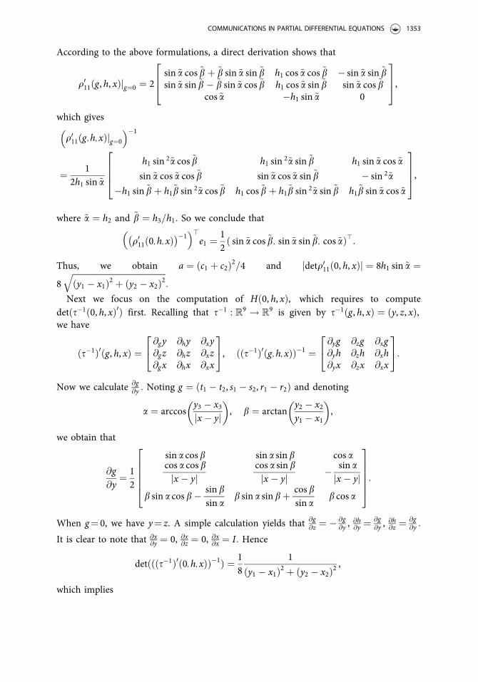
According to the above formulations, a direct derivation shows that

q011ðg, h, xÞjg¼0 ¼ 2sin ~a cos ~b þ ~b sin ~a sin ~b h1 cos ~a cos ~b � sin ~a sin ~bsin ~a sin ~b � ~b sin ~a cos ~b h1 cos ~a sin ~b sin ~a cos ~b

cos ~a �h1 sin ~a 0

264

375,

which gives


� ��1

¼ 12h1 sin ~a

h1 sin 2~a cos ~b h1 sin 2~a sin ~b h1 sin ~a cos ~a

sin ~a cos ~a cos ~b sin ~a cos ~a sin ~b � sin 2~a

�h1 sin ~b þ h1~b sin 2~a cos ~b h1 cos ~b þ h1~b sin 2~a sin ~b h1~b sin ~a cos ~a

2664

3775,

where ~a ¼ h2 and ~b ¼ h3=h1: So we conclude that

q011ð0, h, xÞ� ��1� �>

e1 ¼ 12ð sin ~a cos ~b, sin ~a sin ~b, cos ~aÞ>:

Thus, we obtain a ¼ ðc1 þ c2Þ2=4 and jdetq011ð0, h, xÞj ¼ 8h1 sin ~a ¼8

ffiffiffiffiffiffiffiffiffiffiffiffiffiffiffiffiffiffiffiffiffiffiffiffiffiffiffiffiffiffiffiffiffiffiffiffiffiffiffiffiffiffiffiffiffiðy1 � x1Þ2 þ ðy2 � x2Þ2

q:

Next we focus on the computation of Hð0, h, xÞ, which requires to computedetðs�1ð0, h, xÞ0Þ first. Recalling that s�1 : R9 ! R

9 is given by s�1ðg, h, xÞ ¼ ðy, z, xÞ,we have

ðs�1Þ0ðg, h, xÞ ¼@gy @hy @xy@gz @hz @xz@gx @hx @xx

24

35, ððs�1Þ0ðg , h, xÞÞ�1 ¼

@yg @zg @xg@yh @zh @xh@yx @zx @xx

24

35:

Now we calculate @g@y : Noting g ¼ ðt1 � t2, s1 � s2, r1 � r2Þ and denoting

a ¼ arccosy3 � x3jx � yj

� �, b ¼ arctan

y2 � x2y1 � x1

� �,

we obtain that

@g@y

¼ 12

sin a cosb sin a sin b cos acos a cosbjx � yj

cos a sin bjx � yj � sin a

jx � yjb sin a cos b� sin b

sin ab sin a sin bþ cosb

sin ab cos a

266664

377775:

When g¼ 0, we have y¼ z. A simple calculation yields that @g@z ¼ � @g

@y ,@h@y ¼ @g

@y ,@h@z ¼ @g

@y :

It is clear to note that @x@y ¼ 0, @x@z ¼ 0, @x@x ¼ I: Hence

detðððs�1Þ0ð0, h, xÞÞ�1Þ ¼ 18

1

ðy1 � x1Þ2 þ ðy2 � x2Þ2,

which implies


detððs�1Þ0ð0, h, xÞÞ ¼ 8 ðy1 � x1Þ2 þ ðy2 � x2Þ2� �

:

Substituting these results into (3.31) gives

R3ðx, jÞ ¼ cm

ðR

3eiðc1�c2Þjh�e1 ðx1 � y1Þm1þn1ðx2 � y2Þm2þn2ðx3 � y3Þm3þn3

jx� yjp1þp2

�ffiffiffiffiffiffiffiffiffiffiffiffiffiffiffiffiffiffiffiffiffiffiffiffiffiffiffiffiffiffiffiffiffiffiffiffiffiffiffiffiffiffiffiffiffiðx1 � y1Þ2 þ ðx2 � y2Þ2

q/ðyð0, h, xÞÞdh,

where ðy, z, xÞ ¼ s�1ðg, h, xÞ: Noting det @h@y

� �¼ 1

81ffiffiffiffiffiffiffiffiffiffiffiffiffiffiffiffiffiffiffiffiffiffiffiffiffiffiffiffi

ðx1�y1Þ2þðx2�y2Þ2p , we arrive at

R3ðx, jÞ ¼ C3

ðR

3eiðc1�c2Þjx�yjj ðx1 � y1Þm1þn1ðx2 � y2Þm2þn2ðx3 � y3Þm3þn3

jx� yjp1þp2/ðyÞdy,

which completes the proof. w

To finish this section, we prove the following result that is utilized in the recovery ofthe micro-correlation strength /:

Lemma 3.6. Let V1,V2 � Rd be two open, bounded, and simply connected domains with

positive distance. For some positive integer l and / 2 C10 ðV1Þ, define the integral

TðxÞ ¼ðR

d

1

jx � yjl /ðyÞdy, x 2 V2:

Then TðxÞ, x 2 V2 uniquely determines the function /:

Proof. A simple calculation yields

Dxjx � yj�n ¼ n2jx � yj�n�2, n 2 N,

which implies

DnxTðxÞ ¼ cn

ðV1

1

jx� yjlþ2n /ðyÞdy,

where cn is a constant depending on n. Since T(x) is known in an open set V2 whichhas a positive distance to the support of / 2 C1

0 ðR2Þ, so as DnxTðxÞ, n 2 N is known in

the set V2. A linear combination of DnxTðxÞ shows that the integralð

V1

1

jx � yjl P1

jx� yj2 !

/ðyÞdy (3.32)

is known in the set V2, where PðtÞ ¼PJj¼0 ajt

j is a polynomial of order J 2 N: In

(3.32), by changing the integral variables, we deduceðV1

1

jx� yjlP

1

jx� yj2 !

/ðyÞdy ¼ðr2r1

1rlP

1r2

� �ðjy�xj¼r

/ðyÞdsðyÞdr

¼ðr2r1

1rlP

1r2

� �Sðx, rÞdr

¼ 12

ð 1r21

1r22

PðtÞS x,1ffiffit

p� �

tl�32 dt,

1354 J. LI ET AL.

where Sðx, rÞ ¼ Ðjy�xj¼r/ðyÞdsðyÞ denotes the integral of /ðyÞ along the circle jy� xj ¼r, r1 ¼ miny2V1 jx� yj and r2 ¼ maxy2V1 jx� yj denote the minimum and the maximum

distance between the fixed point x 2 V2 and the domain V1, respectively. Due to / 2C10 ðR2Þ, the function S(x, r) is continuous with respect to r and is compact supported

in the interval ½r1, r2: We obtain S x, 1ffiffit

p� �

tl�32 is continuous in ½r�2

2 , r�21 : Note that the

polynomial function P(t) is dense in Cð½r�22 , r�2

1 Þ, thus the function S x, 1ffiffit

p� �

tl�32 is

uniquely determined which implies S(x, r) is uniquely determined for all r> 0.

Let gðxÞ ¼ e�jxj22 for x 2 R

2, then we have

ðg � /ÞðxÞ ¼ðR

2e�

jx�yj22 /ðyÞdy ¼

ðV1

e�jx�yj2

2 /ðyÞdy

¼ðr2r1

e�r22

ðjy�xj¼r

/ðyÞdydr ¼ðr2r1

e�r22 Sðx, rÞdr:

(3.33)

Since S(x, r) is uniquely determined for all r> 0, we can compute the convolution g � /by (3.33) for x 2 V2: Because V2 is open and g � / is real analytic, hence g � / is knowneverywhere, and the Fourier transform Fðg � /Þ is known everywhere. Since

FgðnÞ ¼ðR

2e�ix�ngðxÞdx ¼

ðR

2e�

jxj22 þix�n� �

dx

¼ðR

2e�

12ðx21þ2ix1n1Þe�

12ðx22þ2ix2n2Þdx

¼ e�12jnj2ðR

e�12ðx1þin1Þ2dx1

ðR

e�12ðx2þin2Þ2dx2

¼ 2pe�12jnj2 ,

we conclude Fg is smooth and non-zero all over R2: Therefore, F/ ¼ Fðg � /Þ=Fg isuniquely determined which shows that / is uniquely determined. w

Remark 3.7. We point out that the proof of Lemma 3.6 requires values integral T to beavailable in an open set. This is the fundamental reason why observational data on alower dimensional manifold or boundary are not sufficient in our main results, i.e.,Theorems 3.10 and 3.12, with the current technique. Similar reasoning applies to theelastic wave equation.

3.3. The two-dimensional case

First we discuss the two-dimensional case and show that the function / in the principlesymbol can be uniquely determined by the scattered field obtained from a single realiza-tion of the random source f. Let us begin with the asymptotic of the Hankel function

Hð1Þn with a large argument. By [44, Eqs. (9.2.7)–(9.2.10)] and [44, Eqs.(5.11.4)], we

have:


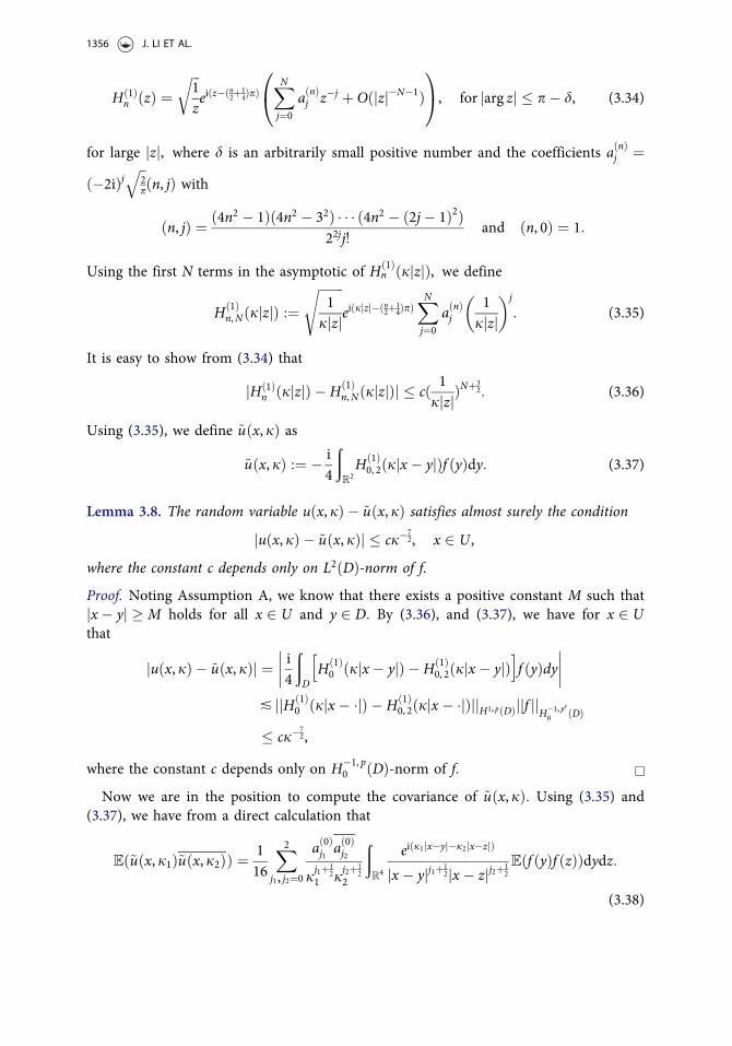
Hð1Þn ðzÞ ¼

ffiffiffi1z

reiðz�ðn2þ1

4ÞpÞXNj¼0

aðnÞj z�j þ Oðjzj�N�1Þ0@

1A, for jarg zj � p� d, (3.34)

for large jzj, where d is an arbitrarily small positive number and the coefficients aðnÞj ¼ð�2iÞj

ffiffi2p

qðn, jÞ with

ðn, jÞ ¼ ð4n2 � 1Þð4n2 � 32Þ � � � ð4n2 � ð2j� 1Þ2Þ22jj!

and ðn, 0Þ ¼ 1:

Using the first N terms in the asymptotic of Hð1Þn ðjjzjÞ, we define

Hð1Þn,NðjjzjÞ :¼

ffiffiffiffiffiffiffiffi1

jjzj

seiðjjzj�ðn2þ1

4ÞpÞXNj¼0

aðnÞj1

jjzj� �j

: (3.35)

It is easy to show from (3.34) that

jHð1Þn ðjjzjÞ �Hð1Þ

n,NðjjzjÞj � cð 1jjzjÞ

Nþ32: (3.36)

Using (3.35), we define ~uðx, jÞ as

~uðx, jÞ :¼ � i4

ðR

2Hð1Þ

0, 2ðjjx� yjÞf ðyÞdy: (3.37)

Lemma 3.8. The random variable uðx, jÞ � ~uðx, jÞ satisfies almost surely the condition

juðx, jÞ � ~uðx, jÞj � cj�72, x 2 U,

where the constant c depends only on L2ðDÞ-norm of f.

Proof. Noting Assumption A, we know that there exists a positive constant M such thatjx� yj � M holds for all x 2 U and y 2 D: By (3.36), and (3.37), we have for x 2 Uthat

juðx, jÞ � ~uðx, jÞj ¼�� i4ðD

Hð1Þ0 ðjjx � yjÞ � Hð1Þ

0, 2ðjjx� yjÞh i

f ðyÞdy��

� jjHð1Þ0 ðjjx� �jÞ � Hð1Þ

0, 2ðjjx � �jÞjjH1, pðDÞjjf jjH�1, p00 ðDÞ

� cj�72,

where the constant c depends only on H�1, p0 ðDÞ-norm of f. w

Now we are in the position to compute the covariance of ~uðx, jÞ: Using (3.35) and(3.37), we have from a direct calculation that

Eð~uðx, j1Þ~uðx, j2ÞÞ ¼ 116

X2j1, j2¼0

að0Þj1 að0Þj2

jj1þ1

21 j

j2þ12

2

ðR

4

eiðj1jx�yj�j2jx�zjÞ

jx � yjj1þ12jx� zjj2þ1

2

Eðf ðyÞf ðzÞÞdydz:

(3.38)

1356 J. LI ET AL.

Since Eð~uðx, j1Þ~uðx, j2ÞÞ is a linear combination of I which satisfies the estimate (3.17),thus the following result is a direct consequence of Lemma 3.4.

Lemma 3.9. For j1, j2 � 1, the estimates

jEð~uðx, j1Þ~uðx, j2ÞÞj � cnðj1 þ j2Þ�ðmþ1Þð1þ jj1 � j2jÞ�n,

jEð~uðx, j1Þ~uðx, j2ÞÞj � cnðj1 þ j2Þ�nð1þ jj1 � j2jÞ�m:

holds uniformly for x 2 U, where n 2 N is arbitrary and cn > 0 is a constant dependingonly on n.

Now we are ready to estimate the order of Eðj~uðx, jÞj2Þ: Setting j1 ¼ j2 ¼ j in(3.38) and applying Lemma 3.5, we obtain

Eðj~uðx, jÞj2Þ ¼ Tð2ÞA ðxÞj�ðmþ1Þ þ Oðj�ðmþ2ÞÞ, (3.39)

where

Tð2ÞA ðxÞ ¼ 1

32p

ðR

2

1jx � yj/ðyÞdy: (3.40)

We are in the position to present the main result for the time-harmonic acoustic waves.

Theorem 3.10. Let the external source f be a microlocally isotropic Gaussian random fieldwhich satisfies Assumption B. Then for all x 2 U, it holds almost surely that

limQ!1

1Q� 1

ðQ1jmþ1juðx, jÞj2dj ¼ Tð2Þ

A ðxÞ: (3.41)

Moreover, the scattering data Tð2ÞA ðxÞ, x 2 U uniquely determines the micro-correlation

strength / through the linear relation (3.40).

Proof. A simple calculation shows that

1Q� 1

ðQ1jmþ1juðx, jÞj2dj

¼ 1Q� 1

ðQ1jmþ1j~uðx, jÞ þ uðx, jÞ � ~uðx, jÞj2dj

¼ 1Q� 1

ðQ1jmþ1j~uðx, jÞj2djþ 1

Q� 1

ðQ1jmþ1juðx, jÞ � ~uðx, jÞj2dj

þ 2Q� 1

ðQ1jmþ1R ~uðx, jÞðuðx, jÞ � ~uðx, jÞÞ

h idj:

It is clear that (3.41) follows as long as we show that

limQ!1

1Q� 1

ðQ1jmþ1j~uðx, jÞj2dj ¼ Tð2Þ

A ðxÞ, (3.42)

limQ!1

1Q� 1

ðQ1jmþ1juðx, jÞ � ~uðx, jÞj2dj ¼ 0, (3.43)

limQ!1

2Q� 1


h idj ¼ 0: (3.44)


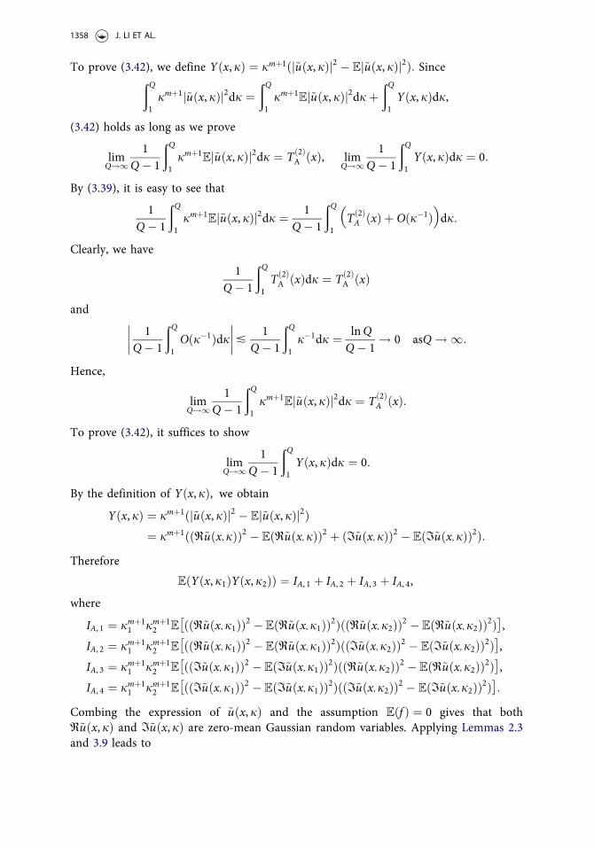
To prove (3.42), we define Yðx, jÞ ¼ jmþ1ðj~uðx, jÞj2 � Ej~uðx, jÞj2Þ: SinceðQ1jmþ1j~uðx, jÞj2dj ¼

ðQ1jmþ1

Ej~uðx, jÞj2djþðQ1Yðx, jÞdj,

(3.42) holds as long as we prove

limQ!1

1Q� 1

ðQ1jmþ1

Ej~uðx, jÞj2dj ¼ Tð2ÞA ðxÞ, lim

Q!11

Q� 1

ðQ1Yðx, jÞdj ¼ 0:

By (3.39), it is easy to see that

1Q� 1

ðQ1jmþ1

Ej~uðx, jÞj2dj ¼ 1Q� 1

ðQ1

Tð2ÞA ðxÞ þ Oðj�1Þ

� �dj:

Clearly, we have

1Q� 1

ðQ1Tð2ÞA ðxÞdj ¼ Tð2Þ

A ðxÞ

and �� 1Q� 1

ðQ1Oðj�1Þdj

�� 1Q� 1

ðQ1j�1dj ¼ lnQ

Q� 1! 0 asQ ! 1:

Hence,

limQ!1

1Q� 1

ðQ1jmþ1

Ej~uðx, jÞj2dj ¼ Tð2ÞA ðxÞ:

To prove (3.42), it suffices to show

limQ!1

1Q� 1


By the definition of Yðx, jÞ, we obtain

Yðx, jÞ ¼ jmþ1ðj~uðx, jÞj2 � Ej~uðx, jÞj2Þ¼ jmþ1ððR~uðx,jÞÞ2 � EðR~uðx, jÞÞ2 þ ðI~uðx,jÞÞ2 � EðI~uðx, jÞÞ2Þ:

Therefore

EðYðx, j1ÞYðx, j2ÞÞ ¼ IA, 1 þ IA, 2 þ IA, 3 þ IA, 4,

where

IA, 1 ¼ jmþ11 jmþ1

2 E ððR~uðx,j1ÞÞ2 � EðR~uðx,j1ÞÞ2ÞððR~uðx, j2ÞÞ2 � EðR~uðx, j2ÞÞ2Þ� �

,


2 E ððR~uðx,j1ÞÞ2 � EðR~uðx,j1ÞÞ2ÞððI~uðx,j2ÞÞ2 � EðI~uðx,j2ÞÞ2Þ� �

,


2 E ððI~uðx, j1ÞÞ2 � EðI~uðx, j1ÞÞ2ÞððR~uðx,j2ÞÞ2 � EðR~uðx,j2ÞÞ2Þ� �

,


2 E ððI~uðx, j1ÞÞ2 � EðI~uðx, j1ÞÞ2ÞððI~uðx, j2ÞÞ2 � EðI~uðx, j2ÞÞ2Þ� �

:

Combing the expression of ~uðx, jÞ and the assumption Eðf Þ ¼ 0 gives that bothR~uðx, jÞ and I~uðx, jÞ are zero-mean Gaussian random variables. Applying Lemmas 2.3and 3.9 leads to

1358 J. LI ET AL.

IA, 1 ¼ 2jmþ11 jmþ1

2 EðR~uðx, j1ÞR~uðx, j2ÞÞ½ 2

¼ 12jmþ11 jmþ1

2 EðRð~uðx,j1Þ~uðx,j2ÞÞ þRð~uðx, j1Þ~uðx,j2ÞÞÞh i2

�j

mþ12

1 jmþ12

2

ðj1 þ j2Þnð1þ jj1 � j2jÞm þ jmþ12

1 jmþ12

2

ðj1 þ j2Þmþ1ð1þ jj1 � j2jÞn

" #2

�1

ð1þ jj1 � j2jÞm þ 1ð1þ jj1 � j2jÞn

� �2:

We can obtain the same estimates for IA, 2, IA, 3, and IA, 4 by the similar arguments.Thus, an application of Lemma 2.4 gives that

limQ!1

1Q� 1


To prove (3.43), we obtain from Lemma 3.8 that�� 1Q� 1

ðQ1jmþ1juðx, jÞ � ~uðx, jÞj2dj

�� 1Q� 1

ðQ1jmþ1j�7dj

¼ 1Q� 1

ðQ1jm�6dj ¼ 1

m� 5Qm�5 � 1Q� 1

! 0 asQ ! 1:

To prove (3.44), by the H€older inequality, we have�� 2Q� 1


h idj

�� 2

Q� 1

ðQ1jmþ1j~uðx, jÞjjuðx, jÞ � ~uðx, jÞjdj

� 21

Q� 1

ðQ1jmþ1j~uðx,jÞj2dj

" #12

1Q� 1

ðQ1jmþ1juðx,jÞ � ~uðx,jÞj2dj

" #12

! 2Tð2ÞA ðxÞ12 � 0 ¼ 0 asQ ! 1:

Hence, (3.42)–(3.44) hold which means that (3.41) holds. The unique determination of

/ by the scattering data Tð2ÞA ðxÞ for x 2 U is a direct consequence of Lemma 3.6. w

3.4. The three-dimensional case

In this subsection, we show that the scattering data obtained from a single realization ofthe random source can determine uniquely the function / in the principle symbol inthe three dimensions. By (3.3) and (3.13), we have

uðx, jÞ ¼ � 14p

ðR

3

eijjx�yj

jx � yj f ðyÞdy,

which yields


Eðuðx, j1Þuðx, j2ÞÞ ¼ 116p2

ðR

6

eiðj1jx�yj�j2jx�zjÞ

jx� yjjx � zj Eðf ðyÞf ðzÞÞdydz: (3.45)

We apply directly Lemma 3.4 and obtain the estimates of Eðuðx, j1Þuðx, j2ÞÞand Eðuðx, j1Þuðx, j2ÞÞ:Lemma 3.11. For j1 � 1, j2 � 1, the following estimates

jEðuðx, j1Þuðx, j2ÞÞj � cnðj1 þ j2Þ�mð1þ jj1 � j2jÞ�n,

jEðuðx, j1Þuðx, j2ÞÞj � cnðj1 þ j2Þ�nð1þ jj1 � j2jÞ�m

holds uniformly for x 2 U, where n 2 N is arbitrary and cn > 0 is a constant dependingonly on n.To derive the relationship between the scattering data and the function / in the prin-

ciple symbol, by setting j1 ¼ j2 ¼ j in (3.45) and using Lemma 3.5, we get

Eðjuðx, jÞj2Þ ¼ Tð3ÞA ðxÞj�m þ Oðj�ðmþ1ÞÞ, (3.46)

where

Tð3ÞA ðxÞ ¼ 1

128p2

ðR

3

1

jx � yj2 /ðyÞdy: (3.47)

Now we are ready to present the main result for the three-dimensional case.

Theorem 3.12. Let the external source f be a microlocally isotropic Gaussian random fieldwhich satisfies Assumption B. Then for all x 2 U, it holds almost surely that

limQ!1

1Q� 1

ðQ1jmjuðx, jÞj2dj ¼ Tð3Þ

A ðxÞ: (3.48)

Moreover, the scattering data Tð3ÞA ðxÞ, x 2 U uniquely determines the micro-correlation

strength / through the linear integral equation (3.47).

Proof. We decompose jmjuðx, jÞj2 into two parts:

jmjuðx, jÞj2 ¼ jmEjuðx, jÞj2 þ Yðx, jÞ,where

Yðx, jÞ :¼ jmðjuðx, jÞj2 � Ejuðx, jÞj2Þ:Clearly,

1Q� 1

ðQ1jmjuðx, jÞj2dj ¼ 1

Q� 1

ðQ1jmEjuðx, jÞj2djþ 1

Q� 1

ðQ1Yðx, jÞdj:

Hence, (3.48) holds as long as we show that

limQ!1

1Q� 1

ðQ1jmEjuðx, jÞj2dj ¼ Tð3Þ

A ðxÞ, limQ!1

1Q� 1

ðQ1Yðx, jÞdj ¼ 0: (3.49)

The second equation in (3.49) can be obtained by a similar argument to the two-dimensionalcase. Using (3.46) gives

1360 J. LI ET AL.

limQ!1

1Q� 1

ðQ1jmEjuðx, jÞj2dj ¼ lim

Q!11

Q� 1

ðQ1ðTð3Þ

A ðxÞ þ Oðj�1ÞÞdj ¼ Tð3ÞA ðxÞ:

Hence, the first equation in (3.49) holds which implies that (3.48) holds. A direct appli-cation of Lemma 3.6 implies that / is uniquely determined by the scattering data

Tð3ÞA ðxÞ for x 2 U: w

4. Elastic waves

This section concerns the direct and inverse source problems for the elastic wave equa-tion in the two- and three-dimensional cases. Following the general theme for theacoustic case presented in Section 3, we discuss the well-posedness of the direct prob-lem and show the uniqueness of the inverse problem. We prove that the direct scatter-ing problem with a distributional source indeed has a unique solution. For the inverseproblem, we assume that each component of the external source is a microlocally iso-tropic Gaussian random field whose covariance operator is a classical pseudo-differentialoperator. Moreover, the principle symbol of the covariance operator of each componentis assumed to be coincided. Our main results are as follows: in either the two- or three-dimensional case, given the scattering data which is obtained from a single realizationof the random source, the principle symbol of the covariance operator can be uniquelydetermined. The technical details differ from acoustic waves due to the different modelequation and Green tensors.

4.1. The direct scattering problem

In this subsection, we introduce the model problem of the random source scattering forelastic waves, and show that the direct problem with a distributional source iswell-posed.Consider the time-harmonic Navier equation in a homogeneous medium

lDuþ ðkþ lÞrr � uþ x2u ¼ f in Rd, (4.1)

where x > 0 is the angular frequency, k and l are the Lame�constants satisfying l > 0

and kþ l > 0, the external source f 2 Cd is a generalized random function supported

in a bounded and simply connected domain D in Rd, and u 2 C

d is the displacementof the random wave field.

Since the problem is imposed in the open domain Rd, an appropriate radiation con-

dition is needed to complete the formulation of the scattering problem. We adopt theKupradze–Sommerfeld radiation condition to describe the asymptotic behavior of thedisplacement field away from the source. According to the Helmholtz decomposition,the displacement u can be decomposed into the compressional part up and the shearpart us :

u ¼ up þ us in Rd n �D:

The Kupradze–Sommerfeld radiation condition requires that up and us satisfy theSommerfeld radiation condition:


limr!1 r

d�12 @rup � ijpup� � ¼ 0, lim

r!1 rd�12 @rus � ijsusð Þ ¼ 0, r ¼ jxj, (4.2)

where

jp ¼ x

ðkþ 2lÞ1=2¼ cpx, js ¼ x

l1=2¼ csx

are known as the compressional and shear wavenumbers with

cp ¼ ðkþ 2lÞ�1=2, cs ¼ l�1=2:

Note that cp and cs are independent of x and cp < cs:In (4.1), the external source f is a vector with components fi, i ¼ 1, :::, d: To achieve

the main results, throughout this section, we assume that each component fi satisfiesthe following condition.

Assumption C. Recall that D � Rd denotes a bounded and simply connected domain, fi

is assumed to be a microlocally isotropic Gaussian random field of the same order m 2½d, d þ 1

2Þ in D. Each covariance operator Cfi is assumed to have the same principle sym-bol /ðxÞjnj�m with / 2 C1

0 ðDÞ and / � 0: Moreover, we assume that EðfiÞ ¼ 0 andEðfifjÞ ¼ 0 if i 6¼ j for i, j ¼ 1, :::, d:

According to Lemma 2.2, if m¼ d, we have f ðx̂Þ 2 H�e, pðDÞ3: Thus it suffices to

show that the scattering problem for such a deterministic, distributional source f 2H�e, pðDÞ3 has a unique solution.

Introduce the Green tensor Gðx, y,xÞ 2 Cd�d for the Navier equation (4.1) which is

given by

Gðx, y,xÞ ¼ 1lUdðx, y, jsÞId þ 1

x2rxr>

x ðUdðx, y, jsÞ � Udðx, y, jpÞÞ, (4.3)

where Id is the d� d identity matrix and Udðx, y, jÞ is the fundamental solution for thed-dimensional Helmholtz equation given in (3.3). Here the notation rxr>

x is given by

rxr>x u ¼ @2

x1x1u @2x1x2u

@2x2x1u @2

x2x2u

" #if d ¼ 2

and

rxr>x u ¼

@2x1x1u @2

x1x2u @2x1x3u

@2x2x1u @2

x2x2u @2x2x3u

@2x3x1u @2

x3x2u @2x3x3u

264

375 if d ¼ 3

for some scalar function u defined in Rd: It is easily verified that the Green tensor

Gðx, y,xÞ is symmetric with respect to the variables x and y.We study the asymptotic expansion of the Green’s tensor Gðx, y,xÞ when jx� yj is

close to zero. For the two-dimensional case, using (3.4)–(3.5) gives

Hð1Þ2 ðtÞ ¼ � 4i

p1t2� ipþ i4p

t2 lnt2þ ci

4p� 3i16p

þ 18

� �t2 þ O t4 ln

t2

� �as t ! 0: (4.4)

1362 J. LI ET AL.

Recall the recurrence relations (3.8), a direct calculation shows that


0 ðjjx� yjÞ,

@xiU2ðx, y, jÞ ¼ �ji4ðxi � yiÞH

ð1Þ1 ðjjx� yjÞjx � yj ,

@2xixjU2ðx, y, jÞ ¼ �ji

4Hð1Þ

1 ðjjx� yjÞjx � yj dij þ j2i

4ðxi � yiÞðxj � yjÞH

ð1Þ2 ðjjx � yjÞjx� yj2 ,

where dij is the Kronecker delta function. Hence, by (3.7) and (4.4), we have

jsHð1Þ1 ðjsjx � yjÞ � jpH

ð1Þ1 ðjpjx� yjÞ ¼ i

pjx� yj j2s ln

jsjx� yj2

� j2p lnjpjx � yj

2

� �

þ 12þ ipc� i

2p

� �ðj2s � j2pÞjx � yj þ O jx � yj3 ln jx � yj

2

� �,

j2sHð1Þ2 ðjsjx� yjÞ � j2pH

ð1Þ2 ðjpjx � yjÞ ¼ i

4pj4s ln

jsjx � yj2

� j4p lnjpjx � yj

2

� �jx � yj2

� ipðj2s � j2pÞ þ

ci4p

� 3i16p

þ 18

� �ðj4s � j4pÞjx � yj2 þ O jx � yj4 ln jx � yj

2

� �,

which gives

@2xixj U2ðx, y,jsÞ � U2ðx, y, jpÞ� �

¼ � i4

1jx � yj jsH

ð1Þ1 ðjsjx� yjÞ � jpH

ð1Þ1 ðjpjx � yjÞ

h idij

þ i4

ðxi � yiÞðxj � yjÞjx� yj2 j2sH

ð1Þ2 ðjsjx� yjÞ � j2pH

ð1Þ2 ðjpjx� yjÞ

h i

¼ 14p

j2s lnjsjx� yj

2� j2p ln

jpjx� yj2

� �dij þ 1

4pðj2s � j2pÞ

ðxi � yiÞðxj � yjÞjx � yj2

� i8

1þ 2ipc� i

p

� �ðj2s � j2pÞdij �

116p

ðxi � yiÞðxj � yjÞ j4s lnjsjx � yj

2� j4p ln

jpjx� yj2

� �

� i4

ci4p

� 3i16p

þ 18

� �ðj4s � j4pÞðxi � yiÞðxj � yjÞ þ O jx� yj2 ln jx� yj

2

� �:

(4.5)

For the three-dimensional case, it follows from direct calculations that

@xiU3ðx, y, jÞ ¼ ðxi � yiÞ4pjx� yj3 e

ijjx�yjðijjx � yj � 1Þ,

@2xixjU3ðx, y, jÞ ¼

jx� yj2dij � 3ðxi � yiÞðxj � yjÞ4pjx� yj5 eijjx�yjðijjx � yj � 1Þ

� j2ðxi � yiÞðxj � yjÞ

4pjx� yj3 eijjx�yj,

which lead to


@2xixjðU3ðx, y, jsÞ � U3ðx, y, jpÞÞ

¼ jx � yj2dij � 3ðxi � yiÞðxj � yjÞ4pjx � yj5 ðeijsjx�yjðijsjx� yj � 1Þ � eijpjx�yjðijpjx � yj � 1ÞÞ

� ðxi � yiÞðxj � yjÞ4pjx � yj3 ðj2s eijsjx�yj � j2pe

ijpjx�yjÞ:

(4.6)

Lemma 4.1. For some fixed x 2 Rd,Gðx, � ,xÞ 2 ðL2locðRdÞ \H1, p

loc ðRdÞÞd�d, where p 2ð1, 2Þ for d¼ 2 and p 2 1, 32

� �for d¼ 3.

Proof. For any fixed x 2 Rd, we choose a bounded domain V � R

d which contains x.Define q :¼ supy2V jx � yj, then we have V � BqðxÞ: For the two-dimensional case,

from (3.6) and (4.5), it is sufficient to show that

lnjx � yj

22 L2ðVÞ, yi � xi

jx � yj2 2 LpðVÞ, 8 p 2 ð1, 2Þ,

which are proved in Lemma 3.1. For the three-dimensional case, it follows from theexpansion of the exponential function et that

j2s eijsjx�yj � j2pe

ijpjx�yj ¼ ðj2s � j2pÞ þ Oðjx � yjÞ,eijsjx�yjðijsjx � yj � 1Þ � eijpjx�yjðijpjx� yj � 1Þ ¼ 1

2ðj2p � j2s Þjx � yj2 þ Oðjx� yj3Þ:

Thus, by (3.11) and (4.6), it is sufficient to prove

1jx � yj 2 L2ðVÞ, yi � xi

jx� yj3 2 LpðVÞ, 8 p 2 1,32

� �,

which can been similarly proved to the three-dimensional case in Lemma 3.1. w

Let V and G be any two bounded domains in Rd: By Lemma 4.1 and the Sobolev

embedding theorem, we have Gðx, � ,xÞ 2 ðHsðVÞÞd�d, where s 2 ð0, 1Þ for d¼ 2 and

s 2 0, 12� �

for d¼ 3. Hence, for any given g 2 H�s0 ðVÞd, in the dual sense, we define the

operator Hx by

ðHxgÞðxÞ ¼ðVGðx, y,xÞ � gðyÞdy, x 2 G,

where the dot is the matrix-vector multiplication. By the similar arguments to [42,Theorem 8.2], we have the following property.

Lemma 4.2. The operator Hx : H�s0 ðVÞd ! HsðGÞd is bounded for s 2 ð0, 1Þ, d ¼ 2

or s 2 0, 12� �

, d ¼ 3:

Theorem 4.3. For some fixed s 2 0, 1� d6

� �and ~p 2 1, d

d�1

� �, assume 0 < e < s, 1 <

p < minð ~pddþ~pðe�1Þ ,

2ddþ2ðe�sÞÞ and 1

p þ 1p0 ¼ 1, then the scattering problem (4.1)–(4.2) with

the source f 2 H�e, p00 ðDÞd attains a unique solution u 2 He, p

loc ðRdÞd given by

1364 J. LI ET AL.

uðx,xÞ ¼ �ðDGðx, y,xÞ � f ðyÞdy: (4.7)

Proof. The uniqueness of the scattering problem (4.1)–(4.2) is obvious. We focus on theexistence. For convenience, we denote the differential operator in the Navier equation by

D�u :¼ lDuþ ðkþ lÞrr � u:Let Br :¼ fy 2 R

d : jyj < rg be a ball which is large enough such that it contains thesupport of f. Denote by � the unit normal vector on the boundary @Br: The generalizedstress vector on @Br is defined by

Pu :¼ l@�uþ ðkþ lÞðr � uÞ�:

Since ~p 2 1, dd�1

� �and 1 < p <

~pddþ~pðe�1Þ , we have 1

~p � 1d <

1p � e

d , by Lemma 4.1 and the

Sobolev embedding theorem, we have Gðx, � ,xÞ 2 ðH1, ~ploc ðRdÞÞd�d � ðHe, p

loc ðRdÞÞd�d:

Since D�uþ x2u ¼ f 2 H�e, p00 ðDÞd, in the sense of distributions, we haveð

Br

Gðx, y,xÞ � ðD�uðyÞ þ x2uðyÞÞdy ¼ðBr

Gðx, y,xÞ � f ðyÞdy:

Define the operator acting on u in the left-hand side of the above equation by SE: For

u 2 C1ðRdÞd, from the divergence theorem, we obtain

ðSEuÞðxÞ ¼ðBr

Gðx, y,xÞ � ðD�uðyÞ þ x2uðyÞÞdy

¼ðBrnBdðxÞ

Gðx, y,xÞ � ðD�uðyÞ þ x2uðyÞÞdyþðBdðxÞ


¼ðBrnBdðxÞ

ðGðx, y,xÞ � D�uðyÞ � D�Gðx, y,xÞ � uðyÞÞdy

þðBdðxÞ


¼ðBdðxÞ


þð@Br[@BdðxÞ

Gðx, y,xÞ � PuðyÞ � PGðx, y,xÞ � uðyÞ� �dsðyÞ,

where d > 0 is a sufficiently small constant. By the mean value theorem, it is easy toverify that

limd!0

ð@BdðxÞ

Gðx, y,xÞ � PuðyÞ � PGðx, y,xÞ � uðyÞ� �dsðyÞ ¼ �uðxÞ

and

limd!0

ðBdðxÞ

Gðx, y,xÞ � ðD�uðyÞ þ x2uðyÞÞdy ¼ 0:


Hence, we obtain

ðSEuÞðxÞ ¼ �uðxÞ þð@Br

Gðx, y,xÞ � PuðyÞ � PGðx, y,xÞ � uðyÞ� �dsðyÞ,

which implies

ðSEuÞðxÞ ¼ �uðxÞ þð@Br

Gðx, y,xÞ � PuðyÞ � PGðx, y,xÞ � uðyÞ� �dsðyÞ:

Since uðyÞ and Gðx, y,xÞ satisfy the Sommerfeld radiation condition, we have

limr!1

ð@Br

Gðx, y,xÞ � PuðyÞ � PGðx, y,xÞ � uðyÞ� �dsðyÞ ¼ 0:

Therefore

uðx,xÞ ¼ �ðDGðx, y,xÞ � f ðyÞdy ¼ �Hxf ðxÞ:

Next is to show that u 2 He, ploc ðRdÞd: By Lemma 4.2, we have that for s 2 0, 1� d

6

� �, the

operator Hx : H�s0 ðDÞd ! Hs

locðRdÞd is bounded. The assumption 1 < p < 2ddþ2ðe�sÞ

implies that 12 þ e�s

d < 1p < 1 which yields 1

2 � sd <

1p � e

d : Thus, due to 0 < e < s, the

Sobolev embedding theorem implies that HsðDÞ is embedded into He, pðDÞ and

H�e, p00 ðDÞ is embedded into H�s

0 ðDÞ: Thus, the operator Hx : H�e, p00 ðDÞd ! He, p

loc ðRdÞd isbounded, which completes the proof. w

4.2. The two-dimensional case

This subsection is devoted to study the two-dimensional case. It is required to derive arelationship between the scattering data and the principle symbol of the covarianceoperator of the component of f. To this end, we need to express the displacement

uðx,xÞ explicitly. Substituting (4.5) into (4.3) gives that uðx,xÞ ¼ ðu1ðx,xÞ, u2ðx,xÞÞ>where

uiðx,xÞ ¼ ui1ðx,xÞ þ ui2ðx,xÞ þ ui3ðx,xÞ þ ui4ðx,xÞ,with

ui1ðx,xÞ ¼ i4l

ðDHð1Þ

0 ðjsjx � yjÞfiðyÞdy,

ui2ðx,xÞ ¼ i4x2

ðD

�jsHð1Þ1 ðjsjx � yjÞ þ jpH

ð1Þ1 ðjpjx� yjÞ

h i 1jx� yj fiðyÞdy,

ui3ðx,xÞ ¼ i4x2

ðD



h i ðxi � yiÞ2jx� yj2 fiðyÞdy,

ui4ðx,xÞ ¼ i4x2

ðD



h i ðx1 � y1Þðx2 � y2Þjx� yj2 fkðyÞdy,

here i¼ 1, 2 and fi, kg ¼ f1, 2g:

1366 J. LI ET AL.

To prove the main result, we need to establish the asymptotic of uðx,xÞ for x ! 1:

Recalling the definition of Hð1Þn,N given in (3.35), we define ~uðx,xÞ ¼ ð~u1ðx,xÞ,

~u2ðx,xÞÞ>, where~uiðx,xÞ ¼ ~ui1ðx,xÞ þ ~ui2ðx,xÞ þ ~ui3ðx,xÞ þ ~ui4ðx,xÞ,

Here

~ui1ðx,xÞ ¼ i4l

ðDHð1Þ

0, 2ðjsjx � yjÞfiðyÞdy,

~ui2ðx,xÞ ¼ i4x2

ðD

�jsHð1Þ1, 3ðjsjx� yjÞ þ jpH

ð1Þ1, 3ðjpjx� yjÞ

h i 1jx� yj fiðyÞdy,

~ui3ðx,xÞ ¼ i4x2

ðD

j2sHð1Þ2, 4ðjsjx� yjÞ � j2pH


h i ðxi � yiÞ2jx� yj2 fiðyÞdy,

~ui4ðx,xÞ ¼ i4x2

ðD

j2sHð1Þ2, 4ðjsjx� yjÞ � j2pH


h i ðx1 � y1Þðx2 � y2Þjx � yj2 fkðyÞdy,

where i¼ 1, 2 and fi, kg ¼ f1, 2g:Lemma 4.4. The random variable uðx,xÞ � ~uðx,xÞ satisfies almost surely the condition

juðx,xÞ � ~uðx,xÞj � cx�72, x 2 U, x > 0,

where the constant c depends only on H�1, p00 ðDÞ2-norm of f.

Proof. By Assumption A, it is known that there exists a positive constant M such thatjx� yj � M holds for any x 2 U and y 2 D: By (3.36), for x 2 U, we have

ju11ðx,xÞ � ~u11ðx,xÞj ¼�� i4l

ðD

Hð1Þ0 ðjsjx� yjÞ � Hð1Þ

0, 2ðjsjx� yjÞh i

f1ðyÞdy��

� jjHð1Þ0 ðjsjx � �jÞ � Hð1Þ

0, 2ðjsjx � �jÞjjH1, pðDÞjjf1jjH�1, p00 ðDÞ

� cx�72,

where the constant c depends only on H�1, p00 ðDÞ-norm of f1.

Similarly, it is easy to verify that

juijðx,xÞ � ~uijðx,xÞj � cx�72 for i ¼ 1, 2, j ¼ 1, 2, 3, 4,

where the constant c depends only on H�1, p00 ðDÞ2-norm of f. Therefore

juðx,xÞ � ~uðx,xÞj �X2i¼1

X4j¼1

juijðx,xÞ � ~uijðx,xÞj � cx�72,

which completes the proof. w

To derive the relationship between the scattering data and the function in the

principle symbol, we need to estimate Eðuðx,x1Þ � uðx,x2ÞÞ for x1 � 1,x2 � 1: By


Lemma 4.4, it reduces to find the estimate of Eð~uðx,x1Þ � ~uðx,x2ÞÞ for x1 � 1,x2 � 1:

Recalling ~uðx,xÞ ¼ ð~u1ðx,xÞ, ~u2ðx,xÞÞ> and (3.35), we have

Eð~uðx,x1Þ � ~uðx,x2ÞÞ ¼ Eð~u1ðx,x1Þ~u1ðx,x2ÞÞ þ Eð~u2ðx,x1Þ~u2ðx,x2ÞÞ

¼X4i, j¼1

ðEð~u1iðx,x1Þ~u1jðx,x2ÞÞ þ Eð~u2iðx,x1Þ~u2jðx,x2ÞÞÞ(4.8)

where

~ui1 x,xð Þ ¼ i4l

ðDH 1ð Þ

0, 2 jsjx � yj� �fi yð Þdy

¼ i4l

ðDj�1

2s jx � yj�1

2ei jsjx�yj�14pð ÞX2

j¼0

a 0ð Þj

1jsjx � yj� �j

fi yð Þdy,

~ui2 x,xð Þ ¼ i4x2

ðD

�jsH1ð Þ1, 3 jsjx� yj� �þ jpH

1ð Þ1, 3 jpjx� yj� �h i 1

jx � yj fi yð Þdy

¼ i4x2

ðD� j

12sjx � yj�3

2ei jsjx�yj�34pð ÞX3

j¼0

a 1ð Þj


fi yð Þdy

þ i4x2

ðDj

12pjx� yj�3

2ei jpjx�yj�34pð ÞX3

j¼0

a 1ð Þj

1jpjx � yj� �j

fi yð Þdy,


ðD

j2sH1ð Þ2, 4 jsjx� yj� �� j2pH

1ð Þ2, 4 jpjx� yj� �h i x1 � y1ð Þ2

jx � yj2 fi yð Þdy

¼ i4x2

ðDj

32sjx� yj�5

2 xi � yið Þ2ei jsjx�yj�54pð ÞX4

j¼0

a 2ð Þj


fi yð Þdy

� i4x2

ðDj

32pjx� yj�5

2 xi � yið Þ2ei jpjx�yj�54pð ÞX4

j¼0

a 2ð Þj

1jpjx � yj� �j

fi yð Þdy,


ðD

j2sH1ð Þ2, 4 jsjx� yj� �� j2pH

1ð Þ2, 4 jpjx� yj� �h i x1 � y1ð Þ x2 � y2ð Þ

jx� yj2 fk yð Þdy

¼ i4x2

ðDj

32sjx� yj�5

2 x1 � y1ð Þ x2 � y2ð Þei jsjx�yj�54pð ÞX4

j¼0

a 2ð Þj

1jsjx� yj� �j

fk yð Þdy

� i4x2

ðDj

32pjx� yj�5

2 x1 � y1ð Þ x2 � y2ð Þei jpjx�yj�54pð ÞX4

j¼0

a 2ð Þj

1jpjx� yj� �j

fk yð Þdy:

1368 J. LI ET AL.

Using the assumption Eðf1f2Þ ¼ 0, we obtain

Eð~ui1ðx,x1Þ~ui4ðx,x2ÞÞ ¼ 0, Eð~ui2ðx,x1Þ~ui4ðx,x2ÞÞ ¼ 0,



and

Eð~ui1ðx,x1Þ~ui1ðx,x2ÞÞ

¼ 116l2

X2j1, j2¼0

að0Þj1 að0Þj2

cj1þj2þ1s x

j1þ12

1 xj1þ1

22

ðR

4

eiðcsx1jx�yj�csx2jx�zjÞ

jx � yjj1þ12jx � zjj2þ1

2

EðfiðyÞfiðzÞÞdydz,

Eð~ui1ðx,x1Þ~ui2ðx,x2ÞÞ ¼ ep2i

16l

X2j1¼0

X3j2¼0

að0Þj1 að1Þj2

xj1þ1

21 x

j2þ32

2

� ÐR

4 � eiðcsx1jx�yj�csx2jx�zjÞ

cj1þj2s

þ eiðcsx1jx�yj�cpx2jx�zjÞ

cj1þ1

2s c

j2�12

p

" #EðfiðyÞfiðzÞÞ


2

dydz,

Eð~ui1ðx,x1Þ~ui3ðx,x2ÞÞ ¼ epi

16l

X2j1¼0

X4j2¼0

að0Þj1 að2Þj2

xj1þ1

21 x

j2þ12

2

� ÐR

4


cj1þj2�1s

� eiðcsx1jx�yj�cpx2jx�zjÞ

cj1þ1

2s c

j2�32

p

" #ðxi � ziÞ2EðfiðyÞfiðzÞÞjx� yjj1þ1

2jx� zjj2þ52

dydz,

Eð~ui2ðx,x1Þ~ui1ðx,x2ÞÞ ¼ e�p2i

16l

X3j1¼0

X2j2¼0

að1Þj1 að0Þj2

xj1þ3

21 x

j2þ12

2

� ÐR

4 � eiðcsx1jx�yj�csx2jx�zjÞ

cj1þj2s

þ eiðcpx1jx�yj�csx2jx�zjÞ

cj1�1

2p c

j2þ12

s

" #EðfiðyÞfiðzÞÞ


2

dydz,

Eð~ui2ðx,x1Þ~ui2ðx,x2ÞÞ ¼ 116

X3j1, j2¼0

að1Þj1 að1Þj2

xj1þ3

21 x

j2þ32

2

� ÐR

4

�eiðcsx1jx�yj�csx2jx�zjÞ

cj1þj2�1s

þ eiðcpx1jx�yj�cpx2jx�zjÞ

cj1þj2�1p


cj1�1

2s c

j2�12

p

� eiðcpx1jx�yj�csx2jx�zjÞ

cj1�1

2p c

j2�12

s

�EðfiðyÞfiðzÞÞ

jx� yjj1þ32jx� zjj2þ3

2

dydz,


Eð~ui2ðx,x1Þ~ui3ðx,x2ÞÞ ¼ ep2i

16

X3j1¼0

X4j2¼0

að1Þj1 að2Þj2

xj1þ3

21 x

j2þ12

2

� ÐR

4

"� eiðcsx1jx�yj�csx2jx�zjÞ

cj1þj2�2s

� eiðcpx1jx�yj�cpx2jx�zjÞ

cj1þj2�2p


cj1�1

2s c

j2�32

p


cj1�1

2p c

j2�32

s

#ðxi � ziÞ2EðfiðyÞfiðzÞÞjx � yjj1þ3

2jx � zjj2þ52

dydz,

Eð~ui3ðx,x1Þ~ui1ðx,x2ÞÞ ¼ e�pi

16l

X4j1¼0

X2j2¼0

að2Þj1 að0Þj2

xj1þ1

21 x

j2þ12

2

� ÐR

4

"eiðcsx1jx�yj�csx2jx�zjÞ

cj1þj2�1s


cj1�3

2p c

j2þ12

s

#ðxi � yiÞ2EðfiðyÞfiðzÞÞjx � yjj1þ5

2jx � zjj2þ12

dydz,

Eð~ui3ðx,x1Þ~ui2ðx,x2ÞÞ ¼ e�p2i

16

X4j1¼0

X3j2¼0

að2Þj1 að1Þj2

xj1þ1

21 x

j2þ32

2

� ÐR

4

"� eiðcsx1jx�yj�csx2jx�zjÞ

cj1þj2�2s

� eiðcpx1jx�yj�cpx2jx�zjÞ

cj1þj2�2p


cj1�3

2s c

j2�12

p


cj1�3

2p c

j2�12

s

#ðxi � yiÞ2EðfiðyÞfiðzÞÞjx� yjj1þ5

2jx� zjj2þ32

dydz,


X4j1, j2¼0

að2Þj1 að2Þj2

xj1þ1

21 x

j2þ12

2

� ÐR

4


cj1þj2�3s


cj1þj2�3p


cj1�3

2s c

j2�32

p


cj1�3

2p c

j2�32

s

#ðxi � yiÞ2ðxi � ziÞ2EðfiðyÞfiðzÞÞ


2

dydz,


X4j1, j2¼0

að2Þj1 að2Þj2

xj1þ1

21 x

j2þ12

2

� ÐR

4


cj1þj2�3s


cj1þj2�3p


cj1�3

2s c

j2�32

p


cj1�3

2p c

j2�32

s

#ðx1 � y1Þðx2 � y2Þðx1 � z1Þðx2 � z2Þ


2

EðfkðyÞfkðzÞÞdydz,

for i¼ 1, 2 and fi, kg ¼ f1, 2g:A direct application of Lemma 3.4 to each item on the right hand side of (4.8) gives

the following lemma.

Lemma 4.5. For x1 � 1,x2 � 1, the following estimates

jEð~uðx,x1Þ � ~uðx,x2ÞÞj � cnðx1 þ x2Þ�m�1ð1þ jx1 � x2jÞ�n

jEð~uðx,x1Þ � ~uðx,x2ÞÞj � cnðx1 þ x2Þ�nð1þ jx1 � x2jÞ�m

1370 J. LI ET AL.

holds uniformly for x 2 U, where n 2 N is arbitrary and cn > 0 is a constant dependingonly on n.

To obtain the relation between the scattering data and the function in the principle

symbol, it is required to estimate the order of Eð~uðx,xÞ � ~uðx,xÞÞ: According to (4.8)

where we set x1 ¼ x2 ¼ x, it reduces to estimate the order of Eð~uij1ðx,xÞ~uij2ðx,xÞÞfor i ¼ 1, 2, j1, j2 ¼ 1, 2, 3, 4: Applying Lemma 3.5 gives that

Eð~ui1ðx,xÞ~ui2ðx,xÞÞ ¼ Oðx�ðmþ2ÞÞ, Eð~ui2ðx,xÞ~ui1ðx,xÞÞ ¼ Oðx�ðmþ2ÞÞ,Eð~ui2ðx,xÞ~ui2ðx,xÞÞ ¼ Oðx�ðmþ2ÞÞ, Eð~ui2ðx,xÞ~ui3ðx,xÞÞ ¼ Oðx�ðmþ2ÞÞ,Eð~ui3ðx,xÞ~ui2ðx,xÞÞ ¼ Oðx�ðmþ2ÞÞ,

and

Eð~ui1ðx,xÞ~ui1ðx,xÞÞ ¼ Nð2Þ1i ðxÞx�ðmþ1Þ þ Oðx�ðmþ2ÞÞ

Eð~ui1ðx,xÞ~ui3ðx,xÞÞ ¼ Nð2Þ2i ðx,xÞx�ðmþ1Þ þ Oðx�ðmþ2ÞÞ



Eð~ui4ðx,xÞ~ui4ðx,xÞÞ ¼ Nð2Þ5i ðx,xÞx�ðmþ1Þ þ Oðx�ðmþ2ÞÞ,

where

Nð2Þ1i ðxÞ ¼ a1

ðR

2

1jx � yj/ðyÞdy,

Nð2Þ2i ðx,xÞ ¼

ðR

2ða2eiðcs�cpÞjx�yjx � a1Þ ðxi � yiÞ2

jx� yj3 /ðyÞdy,

Nð2Þ3i ðx,xÞ ¼

ðR

2ða2eiðcp�csÞjx�yjx � a1Þ ðxi � yiÞ2

jx� yj3 /ðyÞdy,

Nð2Þ4i ðx,xÞ ¼

ðR

2ða3 � 2a2 cos ððcs � cpÞjx � yjxÞÞ ðxi � yiÞ4

jx� yj5 /ðyÞdy,

Nð2Þ5i ðx,xÞ ¼

ðR

2ða3 � 2a2 cos ððcs � cpÞjx � yjxÞÞ ðx1 � y1Þ2ðx2 � y2Þ2

jx � yj5 /ðyÞdy:

Here, a1, a2, and a3 are positive constants given by

a1 ¼ 132p

c3�ms , a2 ¼ ðcscpÞ

32

32p2

cs þ cp

� �m

, a3 ¼ 132p

c3�ms þ c3�m

p

� �:

By (4.8) and a simple calculation, we obtain

Eð~uðx,xÞ � ~uðx,xÞÞ ¼ Tð2ÞE ðxÞx�ðmþ1Þ þ Oðx�ðmþ2ÞÞ, (4.9)

where


Tð2ÞE ðxÞ ¼

X5j¼1

X2i¼1

Nð2Þji ðx,xÞ ¼ a3

ðR

2

1jx � yj/ðyÞdy: (4.10)

Now we are ready to present the main result for elastic waves in the two dimensions.

Theorem 4.6. Let the external source f be a microlocally isotropic Gaussian random vec-tor field which satisfies Assumption C. Then for all x 2 U, it holds almost surely that

limQ!1

1Q� 1

ðQ1xmþ1juðx,xÞj2dx ¼ Tð2Þ

E ðxÞ, (4.11)

where Tð2ÞE ðxÞ is given in (4.10). Moreover, the scattering data Tð2Þ

E ðxÞ, for x 2 U uniquelydetermine the micro-correlation strength / through the linear integral equation (4.10).

Proof. Since

1Q� 1

ðQ1xmþ1juðx,xÞj2dx

¼ 1Q� 1

ðQ1xmþ1j~uðx,xÞ þ uðx,xÞ � ~uðx,xÞj2dx

¼ 1Q� 1

ðQ1xmþ1j~uðx,xÞj2dxþ 1

Q� 1

ðQ1xmþ1juðx,xÞ � ~uðx,xÞj2dx

þ 2Q� 1

ðQ1xmþ1R ~uðx,xÞðuðx,xÞ � ~uðx,xÞÞ

h idx

thus, (4.11) holds as long as we show that

limQ!1

1Q� 1

ðQ1xmþ1j~uðx,xÞj2dx ¼ Tð2Þ

E ðxÞ, (4.12)

limQ!1

1Q� 1

ðQ1xmþ1juðx,xÞ � ~uðx,xÞj2dx ¼ 0, (4.13)

limQ!1

2Q� 1


h idx ¼ 0: (4.14)

To prove (4.12), we denote Yðx,xÞ ¼ xmþ1ðj~uðx,xÞj2 � Eðj~uðx,xÞj2ÞÞ, which yieldsðQ1xmþ1j~uðx,xÞj2dx ¼

ðQ1xmþ1

Eðj~uðx,xÞj2ÞdxþðQ1Yðx,xÞdx:

Hence, (4.12) holds as long as we prove

limQ!1

1Q� 1

ðQ1xmþ1

Eðj~uðx,xÞj2Þdx ¼ Tð2ÞE ðxÞ, lim

Q!11

Q� 1

ðQ1Yðx,xÞdx ¼ 0: (4.15)

Multiplying (4.9) by xmþ1 and integrating with respect to the frequency x in theinternal ð1,QÞ, we arrive at

1Q� 1

ðQ1xmþ1

Eðj~uðx,xÞj2Þdx ¼ 1Q� 1

ðQ1

Tð2ÞE ðxÞ þ Oðxm�3Þ

� �dx:

1372 J. LI ET AL.

It is clear to note that�� 1Q� 1

ðQ1Oðxm�3Þdx

�� 1Q� 1

ðQ1xm�3dx ! 0 as Q ! 1,

where we use the fact that m 2 ½d, d þ 12Þ: Thus, the first equation in (4.15) holds. Now

we focus on the second equation in (4.15) and want to show that

limQ!1

1Q� 1

ðQ1Yðx,xÞdx ¼ 0:

By the definition of Yðx,xÞ,Yðx,xÞ ¼ xmþ1ðj~uðx,xÞj2 � Eðj~uðx,xÞj2ÞÞ

¼ xmþ1ððR~uðx,xÞÞ2 � EðR~uðx,xÞÞ2 þ ðI~uðx,xÞÞ2 � EðI~uðx,xÞÞ2Þ:Therefore,

EðYðx,x1ÞYðx,x2ÞÞ ¼ IE, 1 þ IE, 2 þ IE, 3 þ IE, 4,

where

IE, 1 ¼ xmþ11 xmþ1

2 E ððR~uðx,x1ÞÞ2 � EðR~uðx,x1ÞÞ2ÞððR~uðx,x2ÞÞ2 � EðR~uðx,x2ÞÞ2Þ� �

,


2 E ððR~uðx,x1ÞÞ2 � EðR~uðx,x1ÞÞ2ÞððI~uðx,x2ÞÞ2 � EðI~uðx,x2ÞÞ2Þ� �

,


2 E ððI~uðx,x1ÞÞ2 � EðI~uðx,x1ÞÞ2ÞððR~uðx,x2ÞÞ2 � EðR~uðx,x2ÞÞ2Þ� �

,


2 E ððI~uðx,x1ÞÞ2 � EðI~uðx,x1ÞÞ2ÞððI~uðx,x2ÞÞ2 � EðI~uðx,x2ÞÞ2Þ� �

:

Combing the expression of ~uðx,xÞ and the assumption Eðf1Þ ¼ 0,Eðf2Þ ¼ 0 gives thatR~uðx,xÞ and I~uðx,xÞ are zero-mean Gaussian random variables. Applying Lemmas2.3 and 4.5 leads to

IE, 1 ¼ 2xmþ11 xmþ1

2 EðR~uðx,x1ÞR~uðx,x2ÞÞ½ 2

¼ 12xmþ1

1 xmþ12 EðRð~uðx,x1Þ~uðx,x2ÞÞ þRð~uðx,x1Þ~uðx,x2ÞÞÞh i2

�x

mþ12

1 xmþ12

2

ðx1 þ x2Þnð1þ jx1 � x2jÞm þ xmþ12

1 xmþ12

2

ðx1 þ x2Þmþ1ð1þ jx1 � x2jÞn

" #2

�1

ð1þ jx1 � x2jÞm þ 1ð1þ jx1 � x2jÞn

� �2:

We can obtain the same estimates for IE, 2, IE, 3, and IE, 4 by the similar arguments. Thus,an application of Lemma 2.4 gives

limQ!1

1Q� 1

ðQ1Yðx,xÞdx ¼ 0:

To prove (4.13), from lemma 4.4, we obtain�� 1Q� 1

ðQ1xmþ1

��uðx,xÞ � ~uðx,xÞj2dxj� 1Q� 1

ðQ1xmþ1x�7dx

�1

Q� 1

ðQ1xm�6dx�

1m� 5

Qm�5 � 1Q� 1

! 0 asQ ! 1:


To prove (4.14), by the H€older inequality, we have�� 2Q� 1


h idx

��

2Q� 1

ðQ1xmþ1j~uðx,xÞjjuðx,xÞ � ~uðx,xÞjdx

� 21

Q� 1

ðQ1xmþ1j~uðx,xÞj2dx

" #12

1Q� 1

ðQ1xmþ1juðx,xÞ � ~uðx,xÞj2dx

" #12

! 2Tð2ÞE ðxÞ12 � 0 ¼ 0 asQ ! 1:

The unique determination of by Tð2ÞE ðxÞ for x 2 U is a direct consequence of Lemma 3.6. w

4.3. The three-dimensional case

To derive the linear relation between the scattering data and the function in the prin-ciple symbol, it is required to express the wave field more explicitly than (4.7).

Substituting (4.6) into (4.3) gives the wave field uðx,xÞ ¼ ðu1ðx,xÞ, u2ðx,xÞ, u3ðx,xÞÞ>where each component uiðx,xÞ is given by

uiðx,xÞ ¼ ui1ðx,xÞ þ ui2ðx,xÞ þ ui3ðx,xÞ:Here

ui1ðx,xÞ ¼ 14pl

ðR

3

eijsjx�yj

jx� yj fiðyÞdy,

ui2ðx,xÞ ¼ 14px2

ðR

3

1

jx� yj3 eijsjx�yjðijsjx � yj � 1Þ � eijpjx�yjðijpjx � yj � 1Þh i

fiðyÞdy,

ui3ðx,xÞ ¼ � 14px2

ðR

3

"3ðijsjx� yj � 1Þ

jx � yj2 þ j2s

!eijsjx�yj

� 3ðijpjx � yj � 1Þjx� yj2 þ j2p

!eijpjx�yj

#ðxi � yiÞjx � yj3 ðx� yÞ � f ðyÞdy:

As mentioned above, we need to derive the relationship between the scattering data andthe function / in the principle symbol. For this end, it is required to calculate the

exception Eðuðx,x1Þ � uðx,x2ÞÞ: Noting that uðx,xÞ 2 C3 and each component has

been decomposed into three parts, we obtain

Eðuðx,xÞ � uðx,xÞÞ¼ Eðu1ðx,xÞu1ðx,xÞ þ u2ðx,xÞu2ðx,xÞ þ u3ðx,xÞu3ðx,xÞÞ

¼X3i, j¼1

E u1iðx,xÞu1jðx,xÞ þ u2iðx,xÞu2jðx,xÞ þ u3iðx,xÞu3jðx,xÞ� �

:

(4.16)

To calculate the expectation Eðuðx,x1Þ � uðx,x2ÞÞ, it is required to calculate the itemson the right hand side of (4.16). Using the expression of uijðx,xÞði, j ¼ 1, 2, 3Þ, we havefrom direct calculations that

1374 J. LI ET AL.

Eðui1ðx,x1Þui1ðx,x2ÞÞ ¼ 116p2l2

ðR

6


jx � yjjx� zj EðfiðyÞfiðzÞÞdydz,

Eðui1ðx,x1Þui2ðx,x2ÞÞ ¼ � 116p2lx2

2

ðR

6½eiðcsx1jx�yj�csx2jx�zjÞðicsx2jx � zj þ 1Þ

� eiðcsx1jx�yj�cpx2jx�zjÞðicpx2jx� zj þ 1Þ EðfiðyÞfiðzÞÞjx � yjjx� zj3 dydz,

Eðui1ðx,x1Þui3ðx,x2ÞÞ ¼ 116p2lx2

2

ðR

6

�ð 3

jx � zj2 ðicsx2jx � zj þ 1Þ � c2sx22Þ�

eiðcsx1jx�yj�csx2jx�zjÞ ��

3

jx� zj2 ðicpx2jx� zj þ 1Þ � c2px22

�eiðcsx1jx�yj�cpx2jx�zjÞ

�

� ðxi � ziÞ2jx � yjjx � zj3 EðfiðyÞfiðzÞÞdydz,

Eðui2ðx,x1Þui1ðx,x2ÞÞ ¼ 116p2lx2

1

ðR

6

�ðicsx1jx � yj � 1Þeiðcsx1jx�yj�csx2jx�zjÞ

� ðicpx1jx � yj � 1Þeiðcpx1jx�yj�csx2jx�zjÞ�

EðfiðyÞfiðzÞÞjx � yj3jx� zj dydz,

Eðui2ðx,x1Þui2ðx,x2ÞÞ ¼ 116p2x2

1x22�ð

R6

�ðicsx1jx� yj � 1Þð�icsx2jx � zj � 1Þeiðcsx1jx�yj�csx2jx�zjÞ

þ ðicpx1jx � yj � 1Þð�icpx2jx � zj � 1Þeiðcpx1jx�yj�cpx2jx�zjÞ

� ðicsx1jx� yj � 1Þð�icpx2jx� zj � 1Þeiðcsx1jx�yj�cpx2jx�zjÞ

� ðicpx1jx � yj � 1Þð�icsx2jx� zj � 1Þeiðcpx1jx�yj�csx2jx�zjÞ�

EðfiðyÞfiðzÞÞjx � yj3jx� zj3 dydz,


1x22�ð

R6½ðicsx1jx � yj � 1Þ 3

jx � zj2 ðicsx2jx � zj þ 1Þ þ c2sx22

� �eiðcsx1jx�yj�csx2jx�zjÞ

þ ðicpx1jx � yj � 1Þ 3

jx � zj2 ðicpx2jx � zj þ 1Þ þ c2px22

� �eiðcpx1jx�yj�cpx2jx�zjÞ

� ðicsx1jx� yj � 1Þ 3

jx� zj2 ðicpx2jx� zj þ 1Þ þ c2px22

� �eiðcsx1jx�yj�cpx2jx�zjÞ

� ðicpx1jx � yj � 1Þ 3

jx � zj2 ðicsx2jx� zj þ 1Þ þ c2sx22

� �eiðcpx1jx�yj�csx2jx�zjÞ

� ðxi � ziÞ2jx � yj3jx � zj3 EðfiðyÞfiðzÞÞdydz,


Eðui3ðx,x1Þui1ðx,x2ÞÞ ¼ � 116p2lx2

1�ð

R6

��3

jx � yj2 ðicsx1jx � yj � 1Þ þ c2sx21

�eiðcsx1jx�yj�csx2jx�zjÞ

��

3

jx � yj2 ðicpx1jx� yj � 1Þ þ c2px21

�eiðcpx1jx�yj�csx2jx�zjÞ

�

� ðxi � yiÞ2jx� yj3jx� zjEðfiðyÞfiðzÞÞdydz,


1x22�ð

R6½ðicsx2jx � zj þ 1Þ 3


!eiðcsx1jx�yj�csx2jx�zjÞ

þ ðicpx2jx� zj þ 1Þ 3


!eiðcpx1jx�yj�cpx2jx�zjÞ

� ðicpx2jx� zj þ 1Þ 3


!eiðcsx1jx�yj�cpx2jx�zjÞ

� ðicsx2jx� zj þ 1Þ 3

jx� yj2 ðicpx1jx � yj � 1Þ þ c2px21

!eiðcpx1jx�yj�csx2jx�zjÞ

� ðxi � yiÞ2jx� yj3jx � zj3 EðfiðyÞfiðzÞÞdydz,


1x22

ðR

6

��3


��

3

jx � zj2 ð�icsx2jx � zj � 1Þ þ c2sx22

� �eiðcsx1jx�yj�csx2jx�zjÞ

þ 3


!�

3

jx � zj2 ð�icpx2jx� zj � 1Þ þ c2px22

� �eiðcpx1jx�yj�cpx2jx�zjÞ

��

3


��

3

jx � zj2 ð�icpx2jx� zj � 1Þ þ c2px22

� �eiðcsx1jx�yj�cpx2jx�zjÞ

� ð 3

jx � yj2 ðicpx1jx � yj � 1Þ þ c2px21Þ�

3

jx � zj2 ð�icsx2jx � zj � 1Þ þ c2sx22

� �eiðcpx1jx�yj�csx2jx�zjÞ

�

� ðxi � yiÞðxi � ziÞjx � yj3jx � zj3

X3j¼1

ðxj � yjÞðxj � zjÞEðfjðyÞfjðzÞÞdydz:

Observe the above expressions, it is easy to see that Eðuðx,x1Þ � uðx,x2ÞÞ is a linearcombination of Iðx,x1,x2Þ which is defined by (3.15). A direct application of

1376 J. LI ET AL.

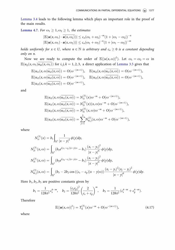
Lemma 3.4 leads to the following lemma which plays an important role in the proof ofthe main results.

Lemma 4.7. For x1 � 1,x2 � 1, the estimates

jEðuðx,x1Þ � uðx,x2ÞÞj � cnðx1 þ x2Þ�mð1þ jx1 � x2jÞ�n

jEðuðx,x1Þ � uðx,x2ÞÞj � cnðx1 þ x2Þ�nð1þ jx1 � x2jÞ�m

holds uniformly for x 2 U, where n 2 N is arbitrary and cn � 0 is a constant dependingonly on n.

Now we are ready to compute the order of Eðjuðx,xÞj2Þ: Let x1 ¼ x2 ¼ x in

Eðuijðx,x1Þuikðx,x1ÞÞ for i, j, k ¼ 1, 2, 3, a direct application of Lemma 3.5 gives that

Eðui1ðx,xÞui2ðx,xÞÞ ¼ Oðx�ðmþ1ÞÞ, Eðui2ðx,xÞui1ðx,xÞÞ ¼ Oðx�ðmþ1ÞÞ,Eðui2ðx,xÞui2ðx,xÞÞ ¼ Oðx�ðmþ1ÞÞ, Eðui2ðx,xÞui3ðx,xÞÞ ¼ Oðx�ðmþ1ÞÞ,Eðui3ðx,xÞui2ðx,xÞÞ ¼ Oðx�ðmþ1ÞÞ,

and

Eðui1ðx,xÞui1ðx,xÞÞ ¼ Nð3Þ1i ðxÞx�m þ Oðx�ðmþ1ÞÞ,

Eðui1ðx,xÞui3ðx,xÞÞ ¼ Nð3Þ2i ðxÞðx,xÞx�m þ Oðx�ðmþ1ÞÞ,

Eðui3ðx,xÞui1ðx,xÞÞ ¼ Nð3Þ3i ðx,xÞx�m þ Oðx�ðmþ1ÞÞ,

Eðui3ðx,xÞui3ðx,xÞÞ ¼X3j¼1

Nð3Þ4i, jðx,xÞx�m þ Oðx�ðmþ1ÞÞ,

where

Nð3Þ1i ðxÞ ¼ b1

ðR

3

1

jx� yj2 /ðyÞdy,

Nð3Þ2i ðx,xÞ ¼

ðR

3ðb2eiðcs�cpÞjx�yjx � b1Þ ðxi � yiÞ2

jx � yj4 /ðyÞdy,

Nð3Þ3i ðx,xÞ ¼

ðR

3ðb2eiðcp�csÞjx�yjx � b1Þ ðxi � yiÞ2

jx � yj4 /ðyÞdy,

Nð3Þ4i, jðx,xÞ ¼

ðR

3ðb3 � 2b2 cos ððcs � cpÞjx � yjxÞÞ ðxi � yiÞ2ðxj � yjÞ2

jx� yj6 /ðyÞdy:

Here b1, b2, b3 are positive constants given by

b1 ¼ 1128p2

c4�ms , b2 ¼ ðcscpÞ2

128p22

cs þ cp

� �m

, b3 ¼ 1128p2

ðc4�ms þ c4�m

p Þ:

Therefore

Eðjuðx,xÞj2Þ ¼ Tð3ÞE ðxÞx�m þ Oðx�ðmþ1ÞÞ, (4.17)

where


Tð3ÞE ðxÞ ¼ ðb3 þ b1Þ

ðR

3

1

jx� yj2 /ðyÞdy: (4.18)

Now we are ready to present the main result of elastic waves for the three-dimen-sional case.

Theorem 4.8. Let the external source f be a microlocally isotropic Gaussian random vec-tor field which satisfies Assumption C. Then for all x 2 U, it holds almost surely that

limQ!1

1Q� 1

ðQ1xmjuðx,xÞj2dx ¼ Tð3Þ

E ðxÞ:

Moreover, the scattering data Tð3ÞE ðxÞ, for x 2 U, uniquely determine the micro-correlation

strength / through the linear relation (4.18).

Proof. Using Lemma 3.6 and (4.17), we may follow the same proof as that for the two-dimensional case. The details are omitted here for brevity. w

5. Conclusion

We have studied an inverse source scattering problem for the two- and three-dimensional Helmholtz equation and Navier equation. The source is assumed to be ageneralized Gaussian random function whose covariance operator is a classical pseudo-differential operator. By an exact expression of the random wave field and microlocalanalysis, we derive a linear integral equation which connects the principle symbol of thecovariance operator and the amplitude of the scattering data generated from a singlerealization of the random source. Based on this relationship, we obtain the uniquenessfor the recovery of the principle symbol of the random source for the Helmholtz andNavier equations. A possible continuation of this work is to investigate the uniquenessfor Maxwell’s equations with a distributional source. Since the Green tensor has ahigher singularity for the Maxwell equations, a new technique must be developed.Another interesting direction is to study the uniqueness for the inverse random sourceproblems in inhomogeneous media, where the analytical Green function or tensor isnot available any more and the present method may not be directly applicable. Wehope to be able to report the progress on these problems in the future.

Funding

The work of TH was funded by the Academy of Finland via the Academy Research Fellow pro-ject, decision number 326961. The research of PL was supported in part by the NSF grantDMS-1912704.

References

[1] Isakov, V. (1989). Inverse Source Problems. Providence, RI: AMS.[2] Arridge, S. (1999). Optical tomography in medical imaging. Inverse Prob. 15(2):R41–R93.

DOI: 10.1088/0266-5611/15/2/022.

1378 J. LI ET AL.

https://doi.org/10.1088/0266-5611/15/2/022

[3] Ammari, H., Bao, G., Fleming, J. (2002). An inverse source problem for Maxwell’s equa-tions in magnetoencephalography. SIAM J. Appl. Math. 62(4):1369–1382. DOI: 10.1137/S0036139900373927.

[4] Fokas, A., Kurylev, Y., Marinakis, V. (2004). The unique determination of neuronal cur-rents in the brain via magnetoencephalogrphy. Inverse Prob. 20(4):1067–1082. DOI: 10.1088/0266-5611/20/4/005.

[5] Nara, T., Oohama, J., Hashimoto, M., Takeda, T., Ando, S. (2007). Direct reconstructionalgorithm of current dipoles for vector magnetoencephalography and electroencephalog-raphy. Phys. Med. Biol. 52(13):3859–3879. DOI: 10.1088/0031-9155/52/13/014.

[6] Marengo, E., Devaney, A. (1999). The inverse source problem of electromagnetics: Linearinversion formulation and minimum energy solution. IEEE Trans. Antennas Propagat.47(2):410–412. DOI: 10.1109/8.761085.

[7] Acosta, S., Chow, S., Taylor, J., Villamizar, V. (2012). On the multi-frequency inversesource problem in heterogeneous media. Inverse Prob. 28(7):075013. DOI: 10.1088/0266-5611/28/7/075013.

[8] Badia, A., Nara, T. (2011). An inverse source problem for Helmholtz’s equation from theCauchy data with a single wave number. Inverse Prob. 27(10):105001. DOI: 10.1088/0266-5611/27/10/105001.

[9] Bao, G., Lu, S., Rundell, W., Xu, B. (2015). A recursive algorithm for multifrequencyacoustic inverse source problems. SIAM J. Numer. Anal. 53(3):1608–1628. DOI: 10.1137/140993648.

[10] Devaney, A., Marengo, E., Li, M. (2007). Inverse source problem in nonhomogeneousbackground media. SIAM J. Appl. Math. 67(5):1353–1378. DOI: 10.1137/060658618.

[11] Eller, M., Valdivia, N. (2009). Acoustic source identification using multiple frequencyinformation. Inverse Prob. 25(11):115005. DOI: 10.1088/0266-5611/25/11/115005.

[12] Zhang, D., Guo, Y. (2015). Fourier method for solving the multi-frequency inverse acous-tic source problem for the Helmholtz equation. Inverse Prob. 31(3):035007. DOI: 10.1088/0266-5611/31/3/035007.

[13] Bleistein, N., Cohen, J. K. (1977). Nonuniqueness in the inverse source problem in acous-tics and electromagnetics. J. Math. Phys. 18(2):194–201. DOI: 10.1063/1.523256.

[14] Devaney, A., Sherman, G. (1982). Nonuniqueness in inverse source and scattering prob-lems. IEEE Trans. Antennas Propagat. 30(5):1034–1037. DOI: 10.1109/TAP.1982.1142902.

[15] Hauer, K.-H., K€uhn, L., Potthast, R. (2005). On uniqueness and non-uniqueness for cur-rent reconstruction from magnetic fields. Inverse Prob. 21(3):955–967. DOI: 10.1088/0266-5611/21/3/010.

[16] Albanese, R., Monk, P. (2006). The inverse source problem for Maxwell’s equations.Inverse Prob. 22(3):1023–1035. DOI: 10.1088/0266-5611/22/3/018.

[17] Bao, G., Lin, J., Triki, F. (2010). A multi-frequency inverse source problem. J. Differ.Equations. 249(12):3443–3465. DOI: 10.1016/j.jde.2010.08.013.

[18] Bao, G., Li, P., Zhao, Y. (2020). Stability for the inverse source problems in elastic andelectromagnetic waves. J. Math. Pures Appl. 134:122–178. DOI: 10.1016/j.matpur.2019.06.006.

[19] Cheng, J., Isakov, V., Lu, S. (2016). Increasing stability in the inverse source problem withmany frequencies. J. Differ. Equations. 260(5):4786–4804. DOI: 10.1016/j.jde.2015.11.030.

[20] Li, P., Yuan, G. (2017). Increasing stability for the inverse source scattering problem withmulti-frequencies. Inverse Probl. Imaging. 11(4):745–759. DOI: 10.3934/ipi.2017035.

[21] Bao, G., Li, P., Lin, J., Triki, F. (2015). Inverse scattering problems with multi-frequencies.Inverse Prob. 31(9):093001. DOI: 10.1088/0266-5611/31/9/093001.

[22] Ammari, H., Bretin, E., Garnier, J., Kang, H., Lee, H., Wahab, A. Mathematical Methodsin Elasticity Imaging. Princeton, NJ: Princeton University Press.

[23] Ciarlet, P. G. (1988). Mathematical Elasticity. Vol. I: Three-Dimensional Elasticity, Studiesin Mathematics and Its Applications. Amsterdam, The Netherlands: North-Holland.

[24] Landau, L. D., Lifshitz, E. M. (1959). Theory of Elasticity. New York, NY: Pergamon Press.


https://doi.org/10.1137/S0036139900373927

https://doi.org/10.1137/S0036139900373927

https://doi.org/10.1088/0266-5611/20/4/005

https://doi.org/10.1088/0266-5611/20/4/005

https://doi.org/10.1088/0031-9155/52/13/014

https://doi.org/10.1109/8.761085

https://doi.org/10.1088/0266-5611/28/7/075013

https://doi.org/10.1088/0266-5611/28/7/075013

https://doi.org/10.1088/0266-5611/27/10/105001

https://doi.org/10.1088/0266-5611/27/10/105001

https://doi.org/10.1137/140993648

https://doi.org/10.1137/140993648

https://doi.org/10.1137/060658618

https://doi.org/10.1088/0266-5611/25/11/115005

https://doi.org/10.1088/0266-5611/31/3/035007

https://doi.org/10.1088/0266-5611/31/3/035007

https://doi.org/10.1063/1.523256

https://doi.org/10.1109/TAP.1982.1142902

https://doi.org/10.1088/0266-5611/21/3/010

https://doi.org/10.1088/0266-5611/21/3/010

https://doi.org/10.1088/0266-5611/22/3/018

https://doi.org/10.1016/j.jde.2010.08.013

https://doi.org/10.1016/j.matpur.2019.06.006

https://doi.org/10.1016/j.matpur.2019.06.006


https://doi.org/10.3934/ipi.2017035

https://doi.org/10.1088/0266-5611/31/9/093001

[25] Michaels, J., Pao, Y.-H. (1985). The inverse source problem for an oblique force on anelastic plate. J. Acoust. Soc. Am. 77(6):2005–2011. DOI: 10.1121/1.391772.

[26] Tittelfitz, J. (2015). An inverse source problem for the elastic wave in the lower-half space.SIAM J. Appl. Math. 75(4):1599–1619. DOI: 10.1137/140971671.

[27] Badieirostami, M., Adibi, A., Zhou, H.-M., Chow, S.-N. (2010). Wiener chaos expansionand simulation of electromagnetic wave propagation excited by a spatially incoherentsource. Multiscale Model. Simul. 8(2):591–604. DOI: 10.1137/090749219.

[28] Devaney, A. (1979). The inverse problem for random sources. J. Math. Phys. 20(8):1687–1691. DOI: 10.1063/1.524277.

[29] Bao, G., Chen, C., Li, P. (2016). Inverse random source scattering problems in severaldimensions. SIAM/ASA J. Uncertainty Quantif. 4(1):1263–1287. DOI: 10.1137/16M1067470.

[30] Bao, G., Chen, C., Li, P. (2017). Inverse random source scattering for elastic waves. SIAMJ. Numer. Anal. 55(6):2616–2643. DOI: 10.1137/16M1088922.

[31] Bao, G., Chow, S.-N., Li, P., Zhou, H. (2013). An inverse random source problem for theHelmholtz equation. Math. Comp. 83(285):215–233. DOI: 10.1090/S0025-5718-2013-02730-5.

[32] Bao, G., Xu, X. (2013). An inverse random source problem in quantifying the elasticmodulus of nanomaterials. Inverse Prob. 29(1):015006. DOI: 10.1088/0266-5611/29/1/015006.

[33] Li, P. (2011). An inverse random source scattering problem in inhomogeneous media.Inverse Prob. 27(3):035004. DOI: 10.1088/0266-5611/27/3/035004.

[34] Li, M., Chen, C., Li, P. (2018). Inverse random source scattering for the Helmholtz equa-tion in inhomogeneous media. Inverse Prob. 34(1):015003. DOI: 10.1088/1361-6420/aa99d2.

[35] Kaipio, J., Somersalo, E. (2005). Statistical and Computational Inverse Problems. NewYork, NY: Springer-Verlag.

[36] Caro, P., Helin, T., Lassas, M. (2019). Inverse scattering for a random potential. Anal.Appl. 17(04):513–567. DOI: 10.1142/S0219530519500015.

[37] Helin, T., Lassas, M., P€aiv€arinta, L. (2017). Inverse acoustic scattering problem in half-space with anisotropic random impedance. J. Differ. Equations. 262(4):3139–3168. DOI:10.1016/j.jde.2016.11.006.

[38] Lassas, M., P€aiv€arinta, L., Saksman, E. (2008). Inverse scattering problem for a two dimen-sional random potential. Commun. Math. Phys. 279(3):669–703. DOI: 10.1007/s00220-008-0416-6.

[39] Jerison, D., Kenig, C. E. (1995). The inhomogeneous Dirichlet problem in Lipschitzdomains. J. Funct. Anal. 130(1):161–219. DOI: 10.1006/jfan.1995.1067.

[40] Cramer, H., Leadbetter, M. (1967). Stationary and Related Stochastic Processes. New York,NY: John Wiley and Sons.

[41] Lebedev, N. N. (1972). Special Functions and Their Applications. New York, NY: DoverPublications, INC.

[42] Colton, D., Kress, R. (2013). Inverse Acoustic and Electromagnetic Scattering Theory. 3rded. Berlin, Germany: Springer.

[43] H€ormander, L. (1985). The Analysis of Linear Partial Differential Operators. Vol. III.Berlin, Germany: Springer-Verlag.

[44] Abramowitz, M., Stegun, I. (1970). Tables of Mathematical Functions. 9th Print. NewYork, NY: Dover.

1380 J. LI ET AL.

https://doi.org/10.1121/1.391772

https://doi.org/10.1137/140971671

https://doi.org/10.1137/090749219

https://doi.org/10.1063/1.524277

https://doi.org/10.1137/16M1067470

https://doi.org/10.1137/16M1067470

https://doi.org/10.1137/16M1088922

https://doi.org/10.1090/S0025-5718-2013-02730-5

https://doi.org/10.1090/S0025-5718-2013-02730-5

https://doi.org/10.1088/0266-5611/29/1/015006

https://doi.org/10.1088/0266-5611/29/1/015006

https://doi.org/10.1088/0266-5611/27/3/035004

https://doi.org/10.1088/1361-6420/aa99d2

https://doi.org/10.1088/1361-6420/aa99d2

https://doi.org/10.1142/S0219530519500015


https://doi.org/10.1007/s00220-008-0416-6

https://doi.org/10.1007/s00220-008-0416-6

https://doi.org/10.1006/jfan.1995.1067

Inverse random source problems for time-harmonic acoustic ...

Documents

Transcript of Inverse random source problems for time-harmonic acoustic ...