Inventory Control Subject to Deterministic Demand Operations Analysis and Improvement 2015 Spring...
69
Dr. Tai-Yue Wang IIM Dept. NCKU Inventory Control Subject to Deterministic Demand Operations Analysis and Improvement 2015 Spring Dr. Tai-Yue Wang Industrial and Information Management Department
-
Upload
horace-scott -
Category
Documents
-
view
217 -
download
2
Transcript of Inventory Control Subject to Deterministic Demand Operations Analysis and Improvement 2015 Spring...

Inventory Control Subject to Deterministic Demand
Operations Analysis and Improvement
2015 Spring
Dr. Tai-Yue WangIndustrial and Information Management Department
National Cheng Kung University

Dr. Tai-Yue Wang IIM Dept. NCKU
Contents
Introduction Types of Inventories Why Inventory? Characteristics of Inventory Systems Relevant Costs The EOQ Model Extension to a Finite Production Rate Quantity Discount Models
Dr. Tai-Yue Wang IIM Dept. NCKU
Contents
Quantity Discount Models Resource-constrained Multiple Product
Systems EOQ Models for Production Planning

Dr. Tai-Yue Wang IIM Dept. NCKU
Overview of Operations Planning Activities

Dr. Tai-Yue Wang IIM Dept. NCKU
Introduction -- Characteristics of Inventory Systems
Demand May Be Known or Uncertain May be Changing or Unchanging in Time
Lead Times - time that elapses from placement of order until it’s arrival. Can assume known or unknown.
Review Time. Is system reviewed periodically or is system state known at all times?

Dr. Tai-Yue Wang IIM Dept. NCKU
Breakdown of the total investment in inventories

Dr. Tai-Yue Wang IIM Dept. NCKU
Treatment of Excess Demand. Backorder all Excess Demand Lose all excess demand Backorder some and lose some
Inventory that changes over time Perishability – 農產品 Obsolescence – 過期之設備備品
Introduction -- Characteristics of Inventory Systems

Dr. Tai-Yue Wang IIM Dept. NCKU
Introduction -- Purposes
Demand is known Methods to control individual item
inventory
Dr. Tai-Yue Wang IIM Dept. NCKU
Types of Inventories
Raw material Components Work-in-Process (WIP) Finished goods

Dr. Tai-Yue Wang IIM Dept. NCKU
Reasons for Holding Inventories
Economies of Scale Uncertainty in delivery leadtimes, supply Speculation-- Changing Costs Over Time Transportation Smoothing Demand Uncertainty Logistics Costs of Maintaining Control System

Dr. Tai-Yue Wang IIM Dept. NCKU
Relevant Costs
Holding Costs - Costs proportional to the quantity of inventory held. Includes:
a) Physical Cost of Space (3%)
b) Taxes and Insurance (2 %)
c) Breakage Spoilage and Deterioration (1%)
*d) Opportunity Cost of alternative investment. (18%)
Note: Since inventory may be changing on a continuous basis, holding cost is proportional to the area under the inventory curve.

Dr. Tai-Yue Wang IIM Dept. NCKU
Relevant Costs (continued)
Ordering Cost (or Production Cost).
Includes both fixed and variable components.
slope = c
K
C(x) = K + cx for x > 0 and =0 for x = 0.

Dr. Tai-Yue Wang IIM Dept. NCKU
Relevant Costs (continued)
Penalty or Shortage Costs. All costs that accrue when insufficient stock is available to meet demand. These include: Loss of revenue for lost demand Costs of bookeeping for backordered demands Loss of goodwill for being unable to satisfy
demands when they occur. Generally assume cost is proportional to number of
units of excess demand.

Dr. Tai-Yue Wang IIM Dept. NCKU
The EOQ Model —The Basic Model
Assumptions:
1. Demand is fixed at l units per unit time.
2. Shortages are not allowed.
3. Orders are received instantaneously. (this will be
relaxed later).

Dr. Tai-Yue Wang IIM Dept. NCKU
The EOQ Model —The Basic Model
Assumptions:
4. Order quantity is fixed at Q per cycle. (can be proven
optimal.)
5. Cost structure:
a) Fixed and marginal order costs (K + cx)
b) Holding cost at h per unit held per unit time.

The EOQ Model —The Basic Model

Dr. Tai-Yue Wang IIM Dept. NCKU
The EOQ Model —The Basic Model
Q is the size of the order At t=0, Q is increased instantaneously from 0 to Q The objective is to choose Q to minimize the
average cost per unit time. In each cycle, the total fixed plus proportional
order cost is C(Q)=K+cQ Since the inventory is consumed by the rate of λ,
the cycle length T is computed by Q/ λ
Dr. Tai-Yue Wang IIM Dept. NCKU
The EOQ Model —The Basic Model
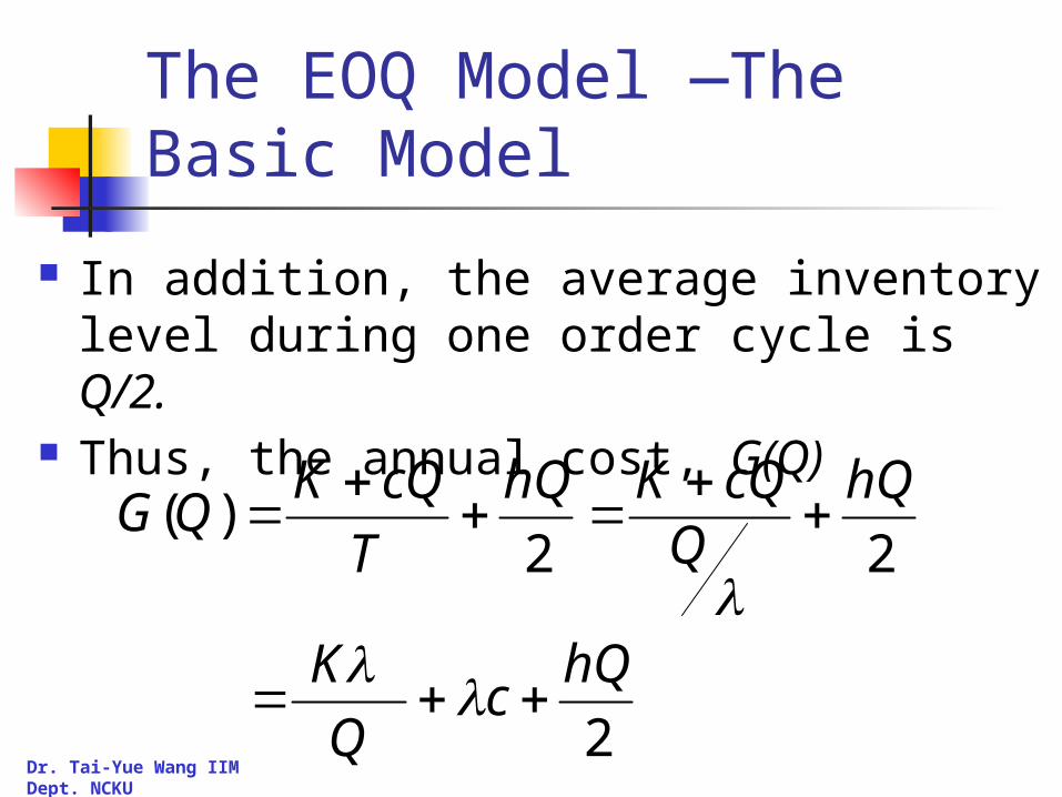
In addition, the average inventory level during one order cycle is Q/2.
Thus, the annual cost, G(Q)
2
22)(
hQc
Q
K
hQQ
cQKhQ
T
cQKQG

Dr. Tai-Yue Wang IIM Dept. NCKU
The EOQ Model —The Basic Model
Thus
0 0/2)(
2//)(3"
2'
QforQKQG
hQKQG
Since G”(q) > 0, G(Q) is a convex function of Q and G’(0)=- ∞ and G’(∞)=h/2, the curve of G(Q) is in next slide.

Dr. Tai-Yue Wang IIM Dept. NCKU
The EOQ Model —The Basic Model

Dr. Tai-Yue Wang IIM Dept. NCKU
The EOQ Model —The Basic Model --Properties of the EOQ Solution
2KQ
h
Q is increasing with both K and and decreasing with h
Q changes as the square root of these quantities Q is independent of the proportional order cost, c.
(except as it relates to the value of h = Ic)

Dr. Tai-Yue Wang IIM Dept. NCKU
The EOQ Model —The Basic Model --Properties of the EOQ Solution
The optimal value of Q occurs where G’(Q)=0
h
KQ
2*
Q* is known as the economic order quantity(EOQ).

Dr. Tai-Yue Wang IIM Dept. NCKU
The EOQ Model —The Basic Model --Example
2KQ
h
Number 2B pencils at campus bookstore are sold at a rate of 60 per week.
The pencil cost is two cents each and sell for 15 cents each. It cost the bookstore $12 to initiate an order and the holding cost are based on annual interest rate of 25 percent.
Please determine the optimal number of pencils for the bookstore to purchase and the time between placement of orders.

Dr. Tai-Yue Wang IIM Dept. NCKU
2KQ
h
The annual demand rate λ=(60)(52)=3,120 The holding cost h=(0.25)(0.02)=0.005
870,3005.0
)120,3)(12)(2(2* h
KQ
The cycle time is T=Q/λ = 3,870/3,120 =1.24 years
The EOQ Model —The Basic Model --Example

Dr. Tai-Yue Wang IIM Dept. NCKU
2KQ
h
In previous example, if the pencils must be ordered four months in advance, we would try to find out when to place order depends on how much inventory on hand.
So we want to reorder at inventory on hand, R, the reorder point.
where is the lead timeR
The EOQ Model — Order Lead time

Dr. Tai-Yue Wang IIM Dept. NCKU
2KQ
h
The EOQ Model — Order Lead time

Dr. Tai-Yue Wang IIM Dept. NCKU
2KQ
h
If the lead time exceeds one cycle, it is more difficult to determine the reorder point
Let EOQ=25, demand rate = 500/year, lead time = 6 weeks,
Cycle time T = 25/500=0.05 year = 2.6 weeks or Lead time = /T = 2.31 cycles
two cycles + 0.31 cycle 0.0155 year
R=0.0155*500=7.75 8
The EOQ Model — Order Lead time

Dr. Tai-Yue Wang IIM Dept. NCKU
2KQ
h
The EOQ Model — Order Lead time
Dr. Tai-Yue Wang IIM Dept. NCKU
2KQ
h
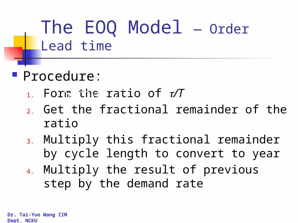
Procedure:1. Form the ratio of /T
2. Get the fractional remainder of the ratio
3. Multiply this fractional remainder by cycle length to convert to year
4. Multiply the result of previous step by the demand rate
The EOQ Model — Order Lead time

Dr. Tai-Yue Wang IIM Dept. NCKU
The EOQ Model — Sensitivity Analysis
Let G(Q) be the average annual holding and set-up cost function given by
and let G* be the optimal average annual cost. Then it can be shown that:
2//)( hQQKQG
*
*
* 2
1)(
Q
Q
Q
Q
G
QG

Dr. Tai-Yue Wang IIM Dept. NCKU
The EOQ Model — Sensitivity Analysis
In general, G(Q) is relatively insensitive to errors in Q
If would results lower average annual cost than a value of
QQQ *
QQQ *
Dr. Tai-Yue Wang IIM Dept. NCKU
The EOQ Model — Example
2KQ
h
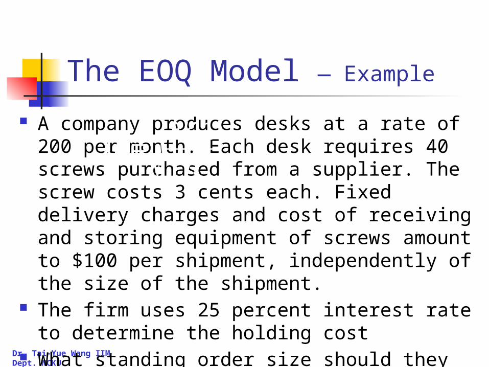
A company produces desks at a rate of 200 per month. Each desk requires 40 screws purchased from a supplier. The screw costs 3 cents each. Fixed delivery charges and cost of receiving and storing equipment of screws amount to $100 per shipment, independently of the size of the shipment.
The firm uses 25 percent interest rate to determine the holding cost
What standing order size should they use?
Dr. Tai-Yue Wang IIM Dept. NCKU
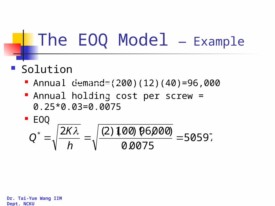
The EOQ Model — Example
2KQ
h
Solution Annual demand=(200)(12)(40)=96,000 Annual holding cost per screw = 0.25*0.03=0.0075 EOQ
505970075.0
)000,96)(100)(2(2* h
KQ

Dr. Tai-Yue Wang IIM Dept. NCKU
EOQ With Finite Production Rate
Suppose that items are produced internally at a rate P > λ. The total cost is
Then the optimal production quantity to minimize average annual holding and set up costs has the same form as the EOQ, namely:
)/1)(2/(/)( PhQQKQG
)/1(
2*
Ph
KQ
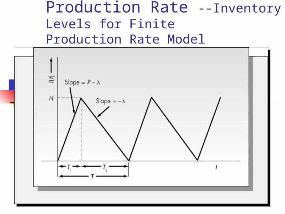
EOQ With Finite Production Rate --Inventory Levels for Finite Production Rate Model

Dr. Tai-Yue Wang IIM Dept. NCKU
EOQ With Finite Production Rate — Example
2KQ
h
Example A company produces EPROM for its customers. The demand
rate is 2,500 units per year. The EPROM is manufactured internally at rate of 10,000 units per year. The cost for initiating the production is $50 and each unit costs the company $2 to manufacture. The cost of holding is based on a 30 percent annual interest rate.
Please determine the optimal size of a production run, the length of each production run, and the average annual cost of holding and setup.
What is the maximum level of the on-hand inventory of the EPROM?

Dr. Tai-Yue Wang IIM Dept. NCKU
EOQ With Finite Production Rate — Example
2KQ
h
Solution: h=0.3*20.6 per unit per year The modified holding cost h’=0.6*(1-2,500/10,000)=0.45
the length of each production run T=Q/=745/2500=0.298 year the average annual cost of holding and setup
74545.0
)500,2)(50)(2(2'
* h
KQ
41.3352/)/1)((/)( *** PhQQKQG

Dr. Tai-Yue Wang IIM Dept. NCKU
EOQ With Finite Production Rate — Example
2KQ
h
Solution: What is the maximum level of the on-hand inventory of the
EPROM?
unitsPQH 559)/1(*

Dr. Tai-Yue Wang IIM Dept. NCKU
Quantity Discount Models
Two kinds of quantity discount: All Units Discounts: the discount is applied to
ALL of the units in the order. Gives rise to an order cost function such as that pictured in Figure 4-9
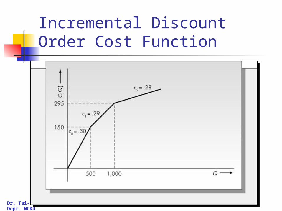
Incremental Discounts: the discount is applied only to the number of units above the breakpoint. Gives rise to an order cost function such as that pictured in Figure 4-10.
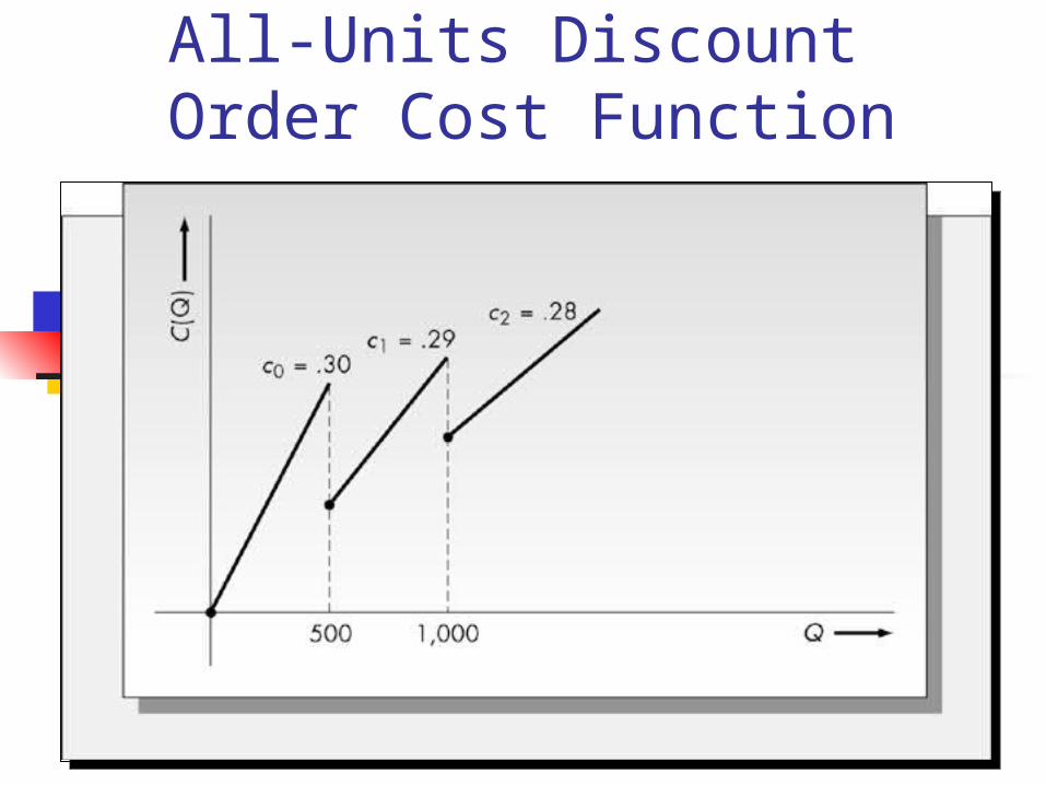
All-Units Discount Order Cost Function
Dr. Tai-Yue Wang IIM Dept. NCKU
Incremental Discount Order Cost Function

Dr. Tai-Yue Wang IIM Dept. NCKU
Quantity Discount Models –all units discount
Trash bag company’s price schedule:
QC
000,1for 28.0
000,1500for 29.0
5000for 30.0
)(
Dr. Tai-Yue Wang IIM Dept. NCKU
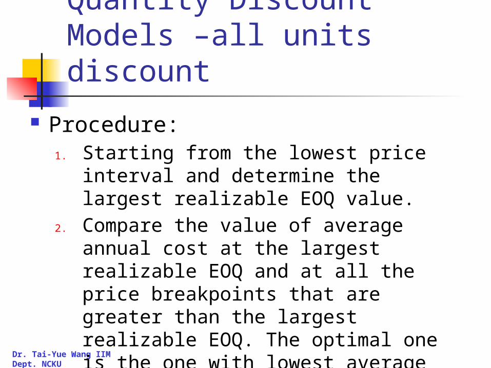
Quantity Discount Models –all units discount
Procedure:1. Starting from the lowest price interval and
determine the largest realizable EOQ value.
2. Compare the value of average annual cost at the largest realizable EOQ and at all the price breakpoints that are greater than the largest realizable EOQ. The optimal one is the one with lowest average annual cost.

Dr. Tai-Yue Wang IIM Dept. NCKU
Quantity Discount Models –all units discount --example
Trash bag company’s price schedule:
For c=0.28, Q*=414 X
c=0.29, Q*=406 X
c=0.30, Q*=400 OK
QC
000,1for 28.0
000,1500for 29.0
5000for 30.0
)(
Dr. Tai-Yue Wang IIM Dept. NCKU
Quantity Discount Models –all units discount --example
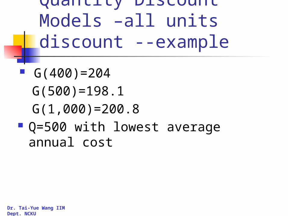
G(400)=204
G(500)=198.1
G(1,000)=200.8 Q=500 with lowest average annual cost

Dr. Tai-Yue Wang IIM Dept. NCKU
Quantity Discount Models –Incremental discount
Trash bag company’s price schedule:
And G(Q) becomes
QC
000,1for )000,1(28.0295
000,1500for )500(29.0150
5000for 30.0
)(
)2/(//)(
cost holding average
cost/Q setupcost/Q material)(
QhQKQQC
QG

Dr. Tai-Yue Wang IIM Dept. NCKU
Quantity Discount Models –Incremental discount
Procedure:1. Find C(Q) equation for all price intervals
2. Substitute C(Q) into G(Q), compute the minimum values of Q for each price intervals
3. Determine which minima computed from previous step are realizable, compute the average annual costs at the realizable EOQ values and pick the lowest one.

Dr. Tai-Yue Wang IIM Dept. NCKU
Quantity Discount Models –Incremental discount --example
Trash bag company’s price schedule:1.
2.
QC
000,1for )000,1(28.0295
000,1500for )500(29.0150
5000for 30.0
)(
)2/](/)(*[//)(
)2/(//)()(
QQQCIQKQQC
QhQKQQCQG

Dr. Tai-Yue Wang IIM Dept. NCKU
Quantity Discount Models –Incremental discount --example
2. 2/*3.0*2.0/600*83.0*600)(0 QQQG
OK -- 4000 Q
)2/(*)/529.0(*2.0
/600*8)/529.0(*600)(1
QQQG
OK-- 5191 Q
)2/(*)/1528.0(*2.0
/600*8)/1528.0(*600)(2
QQQG
XXX-- 7022 Q

Dr. Tai-Yue Wang IIM Dept. NCKU
Quantity Discount Models –Incremental discount --example
3. Compare G0 and G1
204)(0 QG
58.204)(1 QG

Dr. Tai-Yue Wang IIM Dept. NCKU
Quantity Discount Models --Properties of the Optimal Solutions
For all units discounts, the optimal will occur at the bottom of one of the cost curves or at a breakpoint. (It is generally at a breakpoint.). One compares the cost at the largest realizable EOQ and all of the breakpoints succeeding it. (See Figure 4-11).
For incremental discounts, the optimal will always occur at a realizable EOQ value. Compare costs at all realizable EOQ’s. (See Figure 4-12).

All-Units Discount Average Annual Cost Function

Dr. Tai-Yue Wang IIM Dept. NCKU
Average Annual Cost Function for Incremental Discount Schedule

Dr. Tai-Yue Wang IIM Dept. NCKU
Resource Constrained Multi-Product Systems
Consider an inventory system of n items in which the total amount available to spend is C and items cost respectively c1, c2, . . ., cn. Then this imposes the following constraint on the system:
EOQ:
CQcQcQc nn 2211
i
iii h
KQ
2*

Dr. Tai-Yue Wang IIM Dept. NCKU
Resource Constrained Multi-Product Systems
When the condition that
is met, the solution procedure is straightforward.
EOQ
nn hchchc /// 2211
n
iii
ii
EOQcCm
mEOQQ
1
*
/

Dr. Tai-Yue Wang IIM Dept. NCKU
Resource Constrained Multi-Product Systems
If the condition
is not met, one must use an iterative procedure involving Lagrange Multipliers.
nn hchchc /// 2211

Dr. Tai-Yue Wang IIM Dept. NCKU
EOQ Models for Production Planning
Consider n items with known demand rates, production rates, holding costs, and set-up costs. The objective is to produce each item once in a production cycle. j = demand rate for product j Pj= production rate for product j hj = holding cost per unit per unit time for product j Kj= cost of setup the production facility for product j

Dr. Tai-Yue Wang IIM Dept. NCKU
EOQ Models for Production Planning
The goal is to determine the optimal procedure for producing n products on the machine to minimize the cost of holding and setups, and to guarantee that no stock-outs occur during the production cycle.
For the problem to be feasible we must have that
1/1
n
jjj P

Dr. Tai-Yue Wang IIM Dept. NCKU
EOQ Models for Production Planning
We also assume that rotation cycle policy is used. That is, in each cycle, there is exactly one setup for each product, and the products are produced in the same sequence in each production cycle.
Let T be the cycle time, and during time T, exactly one cycle of each product are produced.

Dr. Tai-Yue Wang IIM Dept. NCKU
EOQ Models for Production Planning
So the lot size for product j during time T is
And the average annual cost for product j is
For all products
TQ jj
)2/(/)( 'jjjjjj QhQKQG
n
jjjjjj
n
jj QhQKQG
1
'
1
)2/(/)(
Dr. Tai-Yue Wang IIM Dept. NCKU
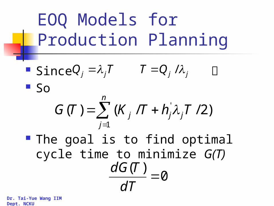
EOQ Models for Production Planning
Since So
The goal is to find optimal cycle time to minimize G(T)
TQ jj
n
jjjj ThTKTG
1
' )2//()(
jjQT /
0)(
dT
TdG

Dr. Tai-Yue Wang IIM Dept. NCKU
EOQ Models for Production Planning
So
However, if setup time is a factor, one needs to check if having enough time for setup and production
n
jjj
n
jj
h
K
T
1
'
1*
2

Dr. Tai-Yue Wang IIM Dept. NCKU
EOQ Models for Production Planning
Let sj be the setup time for product j So
And
So we choose the cycle time T =max(T*, Tmin)
TPTsPQsn
jjjj
n
jjjj
11
)/()/(
min
1
1
/1T
P
s
T n
jjj
n
jj

Dr. Tai-Yue Wang IIM Dept. NCKU
EOQ Models for Production Planning -- Example
A machine serves as a cutting machine for different products. The rotation policy is used and setup cost is proportion to the setup time. Data are followed.
Products Annual Demand(units/year)
Production Rate (units/year)
Setup time(hours)
Variable costs($/unit)
A 4,520 35,800 3.2 40
B 6,600 62,600 2.5 26
C 2,340 41,000 4.4 52
D 2,600 71,000 1.8 18
E 8,800 46,800 5.1 38
F 6,200 71,200 3.1 28
G 5,200 56,000 4.4 31
Dr. Tai-Yue Wang IIM Dept. NCKU
EOQ Models for Production Planning -- Example
The firm estimates that the setup costs amount to an average of $110 per hour, based on the cost of worker time and the cost of forced machine idle time during setups. Holding costs are based on a 22 percent annual interest rate charge.
Please find the optimal cycle time for those products.

Dr. Tai-Yue Wang IIM Dept. NCKU
EOQ Models for Production Planning -- Example
Solution:1. Verify if is valid.
2. Compute the setup costs and modified holding costs
Setup cost K1=$110*3.2=$352, … etc.
Modified holding cost
1/1
n
jjj P
169335.0000,56/200,5...800,35/520,4/1
n
jjj P
69.7)800,35/520,41(*22.0'1 h

Dr. Tai-Yue Wang IIM Dept. NCKU
EOQ Models for Production Planning -- Example
Setup costs(Kj) Modified Holding Costs
352 7.69
275 5.12
484 10.79
198 3.81
561 6.79
341 5.62
484 6.19
Total=2,695
'jh

Dr. Tai-Yue Wang IIM Dept. NCKU
1529.0
200,5*19.6...600,6*12.5520,4*69.7
695,2*22
1
'
1*
n
jjj
n
jj
h
K
T
3. So
4. Assuming 250 working days for one year, that is, the production repeats at roughly 38 working days.
EOQ Models for Production Planning -- Example

Dr. Tai-Yue Wang IIM Dept. NCKU
4. So optimal lots sizes are:
Products Optimal lot sizes for each production run
A 691
B 1,009
C 358
D 398
E 1,346
F 948
G 795
EOQ Models for Production Planning -- Example