Inventory and Prediction of Heavy Duty Diesel Vehicle Emissions

Inventory and Prediction of Heavy-Duty Diesel Vehicle Emissions

By

Justin M. Kern

A THESIS

Submitted toThe College of Engineering and Mineral Resources

atWest Virginia University

in partial fulfillment of the requirementsfor the degree of

Masters of Sciencein

Mechanical Engineering

Nigel N. Clark, Ph.D., ChairChristopher M. Atkinson, Sc.D.

Gregory J. Thompson, Ph.D.Ralph D. Nine, MSME

Department of Mechanical and Aerospace Engineering

Morgantown, West Virginia2000

Keywords: Emissions Inventory, Emissions Prediction, Heavy-Duty Vehicle Emissions

ABSTRACT

INVENTORY AND PREDICTION OF HEAVY-DUTY DIESEL VEHICLE EMISSIONS

By Justin M. Kern

A vehicle emissions inventory is an account of emissions produced by all vehicles in an

area. Many different factors can affect the emissions and the measurement of the emissions that

are used to create an emissions inventory. These factors for heavy-duty diesel vehicles have

been addressed and their relative affect on emissions was evaluated from test data and analytical

analyses. These elements can affect the emissions by a factor of 15 depending on testing

conditions.

One purpose that an emissions database serves is to provide a source for predicting

future emissions for a specific vehicle or many vehicles in a general area. Using a database

directly for prediction is ideal, but no comprehensive data set currently exists that covers all of

the different vehicle and component combinations that exist in current use. Numerical models

can be used to take the existing information about vehicle emissions and calculate the emissions

that would be produced by all the vehicles in an inventory. The Transportable Heavy-Duty

Vehicle Emissions Testing Laboratories at WVU have collected emissions data from heavy-duty

vehicles for approximately 8 years. This existing data were used in an analysis to develop a

method that can produce emissions factors in grams per mile for all heavy-duty vehicles from a

small database of measured emissions. The method developed categorizes the emissions

according to the vehicle speed and acceleration. The WVU emissions data were combined with

truck activity data derived by Battelle Memorial Institute to create emissions factors in grams per

mile that reflects actual driving patterns. These factors were then compared to measured

emissions from the THDVETL and errors were found to be as low as 5%.

iii

AcknowledgementsMany people deserve a lot of thanks and credit for helping me complete this research and

thesis. First, I thank Nigel for giving me the opportunity to attend graduate school and for all the

help and guidance provided during the course of my stay here. Next, I thank the rest of my

committee, Chris Atkinson, Greg Thompson, and Ralph Nine for their help and the time they’ve

devoted to this. Special thanks goes to Ralph for teaching me how the system works, all the

technical help, and for being a good friend.

The Los Alamos National Laboratory and the NCHRP research projects are responsible

for funding the research that led to this monstrosity and they deserve thanks for that.

Thanks to the mobile lab crew for their efforts in collecting the data used for this

research, and thanks to the guys at the ERC for their technical assistance and cynical pessimism.

I couldn’t have endured the this ordeal without the support of the friends I’ve made along

the way, and for that I owe a special thanks to John, Dave, Marcus, Steve, Amy and many more

I’ve failed to mention. The heckling and guidance were both appreciated.

My family has provided support in many ways and for that, thank you very much, Mom

and Dad especially.

iv

Table of ContentsTitle Page..........................................................................................................................................iAbstract............................................................................................................................................iiAcknowledgements....................................................................................................................iiiTable of Contents....................................................................................................................... ivList of Tables .............................................................................................................................viFirst of Figures.........................................................................................................................viiiNomenclature .............................................................................................................................x1. Introduction.........................................................................................................................1

1.1 Exhaust Emissions.......................................................................................................11.2 Origin of Data .............................................................................................................11.3 Technical Description of Laboratory............................................................................2

2. Objectives ...........................................................................................................................53. Literature Review: Previous Prediction Methods ................................................................6

3.1 Current EPA Heavy-Duty Inventory Method ...............................................................63.2 Other Variations of Heavy-Duty Prediction .................................................................83.3 Light-Duty Methods ....................................................................................................8

4. Factors Affecting Compression Ignition Engine Emissions..................................................94.1 Vehicle Class...............................................................................................................94.2 Driving Test Schedules..............................................................................................14

4.2.1 Review of Driving Schedules.................................................................................144.2.2 Test Cycle Emissions Comparison .........................................................................29

4.3 Vehicle Vocations, Weight, and Local Driving Activity.............................................374.4 Fuel Type ..................................................................................................................394.5 Exhaust Aftertreatment..............................................................................................424.6 Vehicle Age...............................................................................................................444.7 Terrain Traveled ........................................................................................................474.8 Injection Timing Variances........................................................................................504.9 Summary of Factors Affecting CI Emissions .............................................................52

5. Methods of Generating Emissions Factors.........................................................................555.1 Certification Data ......................................................................................................555.2 Chassis Dynamometer Data.......................................................................................585.3 Power-Based Emissions Factors ................................................................................615.4 NOX / CO2 Ratios ......................................................................................................685.5 Speed-Acceleration Based .........................................................................................69

6. Methodology of Producing Speed – Acceleration Based Emissions Factors.......................726.1 Speed – Acceleration Profiles of Test Schedules and Creation of the Kern Cycle.......726.2 Vehicle Class and Model Year Divisions ...................................................................766.3 Time Alignment ........................................................................................................766.4 Converting data from ppm to grams per second .........................................................776.5 Calculation of Axle Power.........................................................................................786.6 Proportioning PM to CO............................................................................................786.7 Speed – Acceleration Tables and Methods Used to Fill Empty Cells..........................78

6.7.1 Linear Extrapolation ..............................................................................................816.7.2 Power-Based Extrapolation....................................................................................82

v

6.8 Converting Emissions to Units of g/mile Using Speed-Acceleration Profiles .............827. Results of Emissions Prediction.........................................................................................86

7.1 Comparison of Results...............................................................................................867.2 Incorporation of Various Factors Effecting Emissions ...............................................90

7.2.1 Effect of Age/Mileage-Accumulation on Emissions...............................................907.2.2 Cold Start Emissions..............................................................................................917.2.3 Off-Cycle Operation ..............................................................................................93

7.3 Conclusions and Recommendations...........................................................................98References ..............................................................................................................................100Appendices .............................................................................................................................104Appendix A: Program for developing tables of emissions based on speed-acceleration............105Appendix B: Program for combining SAP’s and emissions data................................................119Appendix C: Program for predicting emissions using the grams/second emissions factors.......124

vi

List of TablesTable 4.1 American Automotive Manufacturers Association (AAMA) Vehicle

Classifications [Merrion, 1994].Table 4.2 Heavy-Duty engine emission standards [EPA, 1997].Table 4.3 EPA emission standards for model year 2004 and later heavy-duty diesel engines.Table 4.4 Power required for a pick-up truck and a tractor truck.Table 4.5 Engine data for class comparison.Table 4.6 Test results for two different vehicles with the same model engine.Table 4.7 Calculated parameters of the various synthesized cycles and routes.Table 4.8 Calculated parameters of the actual cycles.Table 4.9 Engine test data from the FTP cycle on a Navistar engine.Table 4.10 NFRAQS test vehicle #17 emissions test results.Table 4.11 NOX emissions for each cycle (Flint Bus).Table 4.12 CO emissions for each cycle (Flint Bus).Table 4.13 HC emissions for each cycle (Flint Bus).Table 4.14 PM emissions for each cycle (Flint Bus).Table 4.15 NYGT cycle and CBD cycle emissions test results.Table 4.16 CSHVR and CBD cycle emissions test results.Table 4.17 Combined survey data from Roadway and Overnite tractors.Table 4.18 Emission results from varied test weights for a bus.Table 4.19 Emissions comparison of varied concentrations of biodiesel.Table 4.20 Chassis emissions comparison of D2 diesel and F-T fuel.Table 4.21 Engine emissions comparison of various fuels.Table 4.22 Emissions results for comparison of exhaust aftertreatments.Table 4.23 Vehicle specifications and emissions for vehicle age comparison.Table 4.24 Emissions from one vehicle as mileage accumulated.Table 4.25 Constants used for terrain modeling.Table 4.26 Results of the terrain modeling.Table 5.1 Constants used in the road load equation.Table 5.2 Results from the power-based emissions prediction.Table 6.1 Number of test sequences in WVU database based on weight class and model

year.Table 6.2 NOX emissions data grouped according to speed and three acceleration bins for

1997 transit buses.Table 6.3 NOX emissions data grouped according to speed and multiple acceleration bins for

1997 transit buses. (ND = No Data)Table 6.4 NOX Emissions data grouped according to speed and acceleration of the vehicle

for 1998 combination tractor trucks.Table 6.5 Combination truck emissions factors (grams per mile).Table 7.1 Predicted emissions using the speed-acceleration method from one test schedule.Table 7.2 Predicted NOX emissions using the speed-acceleration method from all 1998

tractor truck emissions using the CSHVR (average speed = 14.9 mph).Table 7.3 Predicted NOX emissions using the speed-acceleration method from all 1998

tractor truck emissions using the 5-Mile Route (average speed = 20.1 mph).

vii

Table 7.4 Predicted NOX emissions using the speed-acceleration method from all 1994 to1997 tractor truck emissions using the 5-Mile Route (average speed = 19.9 mph).


Table 7.6 Predicted NOX emissions using the speed-acceleration method from all 1998tractor truck emissions using the CSHVR (average speed = 14.9 mph).

Table 7.7 Predicted NOX emissions using the speed-acceleration method from all 1994 to1997 tractor truck emissions using the WVU 5-Mile Route (average speed = 19.9mph).

Table 7.8 Mileage accumulation data for a 1989 transit bus powered by a DDC 6V-92TAengine rated at 277 hp.

Table 7.9 Example of penalty ratio and NOX emissions per cold start for different lengths oftime considered for cold operation.

viii

First of FiguresFigure 4.1 Central Business District Cycle speed versus time plot.Figure 4.2 Speed versus time for a bus following the CBD cycle.Figure 4.3 Speed versus time plot for the WVU 5-Peak Cycle.Figure 4.4 Speed versus time for a Flint transit bus following the WVU 5-Peak Cycle.Figure 4.5 Speed versus time for a Flint transit bus driving the WVU 5-Mile Route.Figure 4.6 Speed versus time for a truck with a low power-to-weight ratio driving the WVU

5-Mile Route.Figure 4.7 New York Garbage Truck Cycle speed versus time plot.Figure 4.8 Example of a refuse truck driving the New York Garbage Truck Cycle, speed

versus time plot.Figure 4.9 Engine cycle known as the Road Certification Test speed versus time plot.Figure 4.10 New York Bus Cycle speed versus time plot.Figure 4.11 Speed versus time for a transit bus following the New York Bus Cycle.Figure 4.12 EPA Urban Dynamometer Driving Schedule for heavy-duty vehicles (Test-D)

speed versus time plot.Figure 4.13 Speed versus time for a transit bus following Test-D.Figure 4.14 City Suburban Heavy Vehicle Route speed versus time plot.Figure 4.15 Speed versus time for the FTP engine cycle.Figure 4.16 Torque versus time for the FTP.Figure 4.17 Visual comparison of cycles effect on NOX emissions.Figure 4.18 Visual comparison of cycles effect on CO emissions.Figure 4.19 Visual comparison of cycles effect on HC emissions.Figure 4.20 Visual comparison of cycles effect on PM emissions.Figure 4.21 Normalized PM emissions results comparison for different fuel types.Figure 4.22 Smoothed axle power versus shifted NOX as used for terrain modeling.Figure 4.23 Smoothed axle power versus shifted NOX showing bifurcation of data.Figure 4.24 Effect of various factors on particulate matter emissions.Figure 4.25 Effect of various factors on nitrogen oxides emissions.Figure 5.1 Plot of vehicle NOX emissions versus model year using the data from Machiele

(1988).Figure 5.2 NOX emissions of 19 test schedules on one truck.Figure 5.3 Emissions data form the 1996 transit bus on different test weights and test cycles.Figure 5.4 Vehicle NOX emissions versus model year for CBD Cycle using data from chassis

laboratory testing.Figure 5.5 Continuous NOX emissions for a heavy-duty vehicle following the City/Suburban

Heavy Vehicle Route (CSHVR).Figure 5.6 Continuous NOX versus power for a tanker truck tested on the CBD Cycle.Figure 5.7 Plot of Bifurcation of NOX emissions from chassis testing.Figure 5.8 Plot and best fit curve for low NOX mode of the Flint bus driving the CBD Cycle.Figure 5.9 NOX divided by CO2 values for 5 consecutive test runs of the CBD Cycle.Figure 5.10 Speed versus acceleration for transit bus driving the CBD Cycle.Figure 5.11 Speed versus acceleration for a transit bus driving the CSHVR.Figure 6.1 Plot of speed versus acceleration for a tractor truck driven on the WVU 5-Mile

Route.

ix

Figure 6.2 Plot of speed versus acceleration for a tractor truck driven on the City/SuburbanHeavy Vehicle Route.

Figure 6.3 Plot of speed versus acceleration for a tractor truck driven on Test-D.Figure 6.4 Speed versus acceleration for a transit bus driven on the CBD cycle.Figure 6.5 Speed versus acceleration for the Kern Cycle driven by a transit bus.Figure 6.6 Scheduled speed versus time for the Kern cycle.Figure 6.7 Continuous power and emissions versus time for a test run on the Kern Cycle

showing emissions delay.Figure 6.8 Plot of NOX emissions factors for 1998 and current model year tractor trucks.Figure 6.9 Plot of NOX emissions factors for 1994 to 1997 model year tractor trucks.Figure 7.1 Plot of the difference between cold and hot NOX emissions for an FTP.Figure 7.2 A class 8 tractor truck driving the WVU 5-Mile Route showing off-cycle

emissions at the end of the 2nd, 4th, and 5th peaks.Figure7.3 A class 8 tractor truck driving the WVU 5-Mile Route showing possible off-cycle

emissions at the end of the 2nd and 3rd peaks.Figure 7.4 Plot of NOX versus power which displays the off-cycle operation.Figure 7.5 NOX versus power for a vehicle driving the CBD Cycle showing high and low

NOX operation.Figure 7.6 Continuous NOX emissions for a vehicle driving the CBD Cycle showing off-

cycle operation on the 6th, 7th, 8th, and 14th peaks.

x

NomenclatureAAMA American Automotive Manufacturers AssociationASAE American Society of Agriculture EngineersASME American Society of Mechanical EngineersBD BiodieselBSFC Brake Specific Fuel ConsumptionCARB California Air Resources BoardCBD Central Business DistrictCFR Code of Federal RegulationsCNG Compressed natural gasCO Carbon monoxideCO2 Carbon dioxideCRT Continuously Regenerating TrapCSHVR City Suburban Heavy Vehicle RouteD2 Number 2 dieselDDC Detroit Diesel CorporationEGR Exhaust Gas RecirculationEMFAC CARB’s emissions factor programEPA Environmental Protection AgencyF-T Fuel Fischer-Tropsch FuelFTP Federal Test ProcedureGVW Gross Vehicle WeightGVWR Gross Vehicle Weight RatingHC HydrocarbonsIB IsobutanolMG Moss Gas FuelMOBILE5 EPA’s emissions factor programNCHRP National Cooperative Highway Research ProgramND No dataNFRAQS Northern Front Range Air Quality StudyNMHC Non-methane hydrocarbonsNOX oxides of nitrogenNREL National Renewable Energy LaboratoryNYGTC New York Garbage Truck CyclePART5 EPA’s PM emissions factor programPM particulate matterppm parts per millionSAE Society of Automotive EngineersSAP speed - acceleration profileSOF soluble organic fractionTEOM Tapered Element Oscillating MicrobalanceTEST-D Urban Dynamometer Driving Schedule defined by 40 CFR 86THDVETL Transportable Heavy-Duty Vehicle Emissions Testing LaboratoryVMT vehicle miles traveledWVU West Virginia University

1

1. Introduction1.1 Exhaust Emissions

Diesel engines are the most efficient internal combustion engine available today and are

currently the main power source for heavy-duty on-road and off-road vehicles. Recent concerns

about personal and environmental health have brought the subject of exhaust emissions of these

vehicles to public awareness. The United States Environmental Protection Agency (EPA) has set

regulations limiting the production of certain chemical species that emit from diesel engines.

The two species of primary interest are oxides of nitrogen (NOX) and particulate matter (PM).

NOX contributes to the production of smog in urban areas and PM has been targeted as a

carcinogen. Heavy-duty diesel engines are the largest source of diesel PM in the United States.

The total diesel PM emissions for 1997 have been estimated by the EPA at 516 thousand tons

nationwide. Emissions inventories are employed to gain an accurate estimate of the extent of

emissions impact on the environment. Emissions inventories use existing data about different

emissions sources, and the existing data for heavy-duty vehicle emissions is not comprehensive,

which makes accurate inventories from these mobile sources difficult when limited by this data.

A mathematical prediction scheme to predict emissions missing from the measured data replaces

comprehensive testing needed to complete an inventory.

1.2 Origin of Data

The heavy-duty vehicle emissions data used in this analysis were acquired using West

Virginia University’s Transportable Heavy-Duty Vehicle Emissions Testing Laboratories

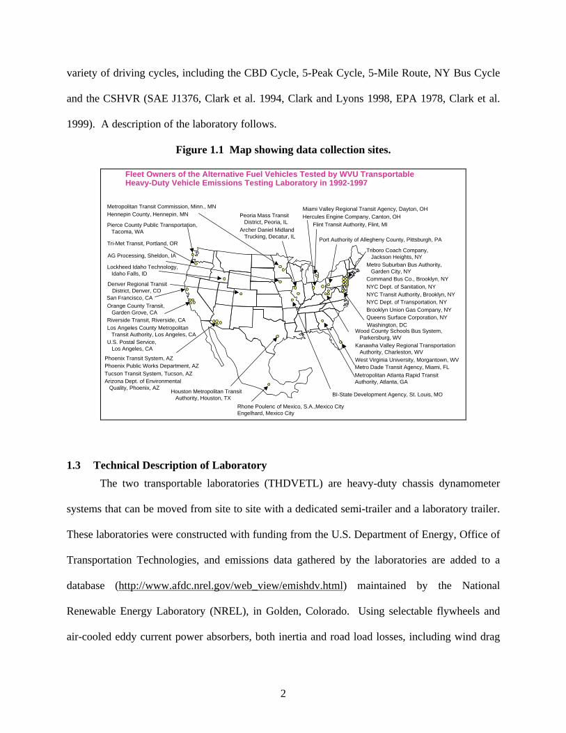
(THDVETL). These two laboratories have collected data across the nation (see Figure 1.1)

primarily to gather data on performance of alternately fueled trucks and buses for the U.S.

Department of Energy, Office of Transportation Technologies. In doing so, substantial

information was gathered from diesel control vehicles. Vehicles were characterized using a

2

variety of driving cycles, including the CBD Cycle, 5-Peak Cycle, 5-Mile Route, NY Bus Cycle

and the CSHVR (SAE J1376, Clark et al. 1994, Clark and Lyons 1998, EPA 1978, Clark et al.

1999). A description of the laboratory follows.

Figure 1.1 Map showing data collection sites.

Fleet Owners of the Alternative Fuel Vehicles Tested by WVU TransportableHeavy-Duty Vehicle Emissions Testing Laboratory in 1992-1997

Pierce County Public Transportation, Tacoma, WA

Metropolitan Transit Commission, Minn., MNHennepin County, Hennepin, MN

Denver Regional Transit District, Denver, CO

Orange County Transit, Garden Grove, CARiverside Transit, Riverside, CALos Angeles County Metropolitan Transit Authority, Los Angeles, CAU.S. Postal Service, Los Angeles, CA

Phoenix Transit System, AZPhoenix Public Works Department, AZTucson Transit System, Tucson, AZArizona Dept. of Environmental Quality, Phoenix, AZ

Houston Metropolitan Transit Authority, Houston, TX

Wood County Schools Bus System, Parkersburg, WVKanawha Valley Regional Transportation Authority, Charleston, WVWest Virginia University, Morgantown, WV

Triboro Coach Company, Jackson Heights, NYMetro Suburban Bus Authority, Garden City, NYCommand Bus Co., Brooklyn, NYNYC Dept. of Sanitation, NYNYC Transit Authority, Brooklyn, NYNYC Dept. of Transportation, NYBrooklyn Union Gas Company, NYQueens Surface Corporation, NY

Miami Valley Regional Transit Agency, Dayton, OHHercules Engine Company, Canton, OHPeoria Mass Transit

District, Peoria, ILArcher Daniel Midland Trucking, Decatur, IL

AG Processing, Sheldon, IA

Tri-Met Transit, Portland, OR

BI-State Development Agency, St. Louis, MO

Metro Dade Transit Agency, Miami, FLMetropolitan Atlanta Rapid TransitAuthority, Atlanta, GA

Port Authority of Allegheny County, Pittsburgh, PA

Flint Transit Authority, Flint, MI

Lockheed Idaho Technology, Idaho Falls, ID

Washington, DC

San Francisco, CA

Rhone Poulenc of Mexico, S.A.,Mexico CityEngelhard, Mexico City

1.3 Technical Description of Laboratory

The two transportable laboratories (THDVETL) are heavy-duty chassis dynamometer

systems that can be moved from site to site with a dedicated semi-trailer and a laboratory trailer.

These laboratories were constructed with funding from the U.S. Department of Energy, Office of

Transportation Technologies, and emissions data gathered by the laboratories are added to a

database (http://www.afdc.nrel.gov/web_view/emishdv.html) maintained by the National

Renewable Energy Laboratory (NREL), in Golden, Colorado. Using selectable flywheels and

air-cooled eddy current power absorbers, both inertia and road load losses, including wind drag

3

and rolling resistance, are simulated by the laboratories. Power is taken directly from the

drivewheels of the tested vehicle via hub adapters while the vehicle runs on free-spinning rollers.

Hub torque, vehicle speed, engine speed, and gaseous emissions data can be logged continuously

during a test through use of a full scale exhaust dilution tunnel, with heated probes and sample

lines and analyzers for carbon monoxide (CO), oxides of nitrogen (NOX) and hydrocarbons

(HC). Particulate matter (PM) is determined gravimetrically by collecting the PM on 70mm

diameter filters. The two laboratories have previously been correlated with one another, and

both laboratories were used to collect data that were used in this analysis.

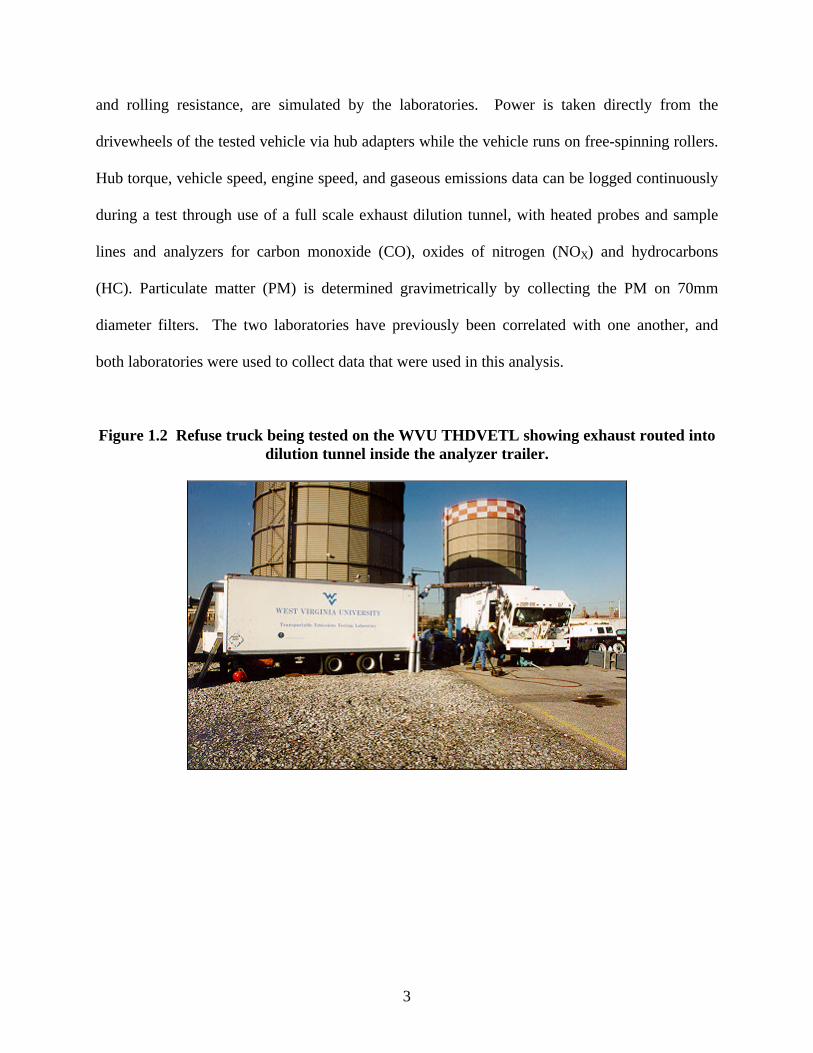
Figure 1.2 Refuse truck being tested on the WVU THDVETL showing exhaust routed intodilution tunnel inside the analyzer trailer.

4

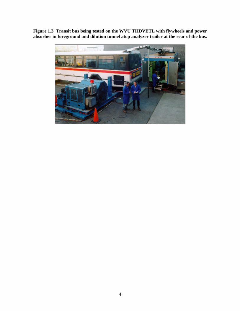
Figure 1.3 Transit bus being tested on the WVU THDVETL with flywheels and powerabsorber in foreground and dilution tunnel atop analyzer trailer at the rear of the bus.

5

2. ObjectivesThe objectives of this analysis include identifying the factors, vehicle components, and

testing procedures that effect the measured exhaust emissions of heavy-duty vehicles. These

observations were made from chassis dynamometer data and were meant to provide guidelines

for processing this data into a useful form for emissions prediction. Data comparisons and

analytical modeling were used to determine the relative effect of each factor on the measured

exhaust emissions. Next, a method to predict emissions for a wide variety of vehicles from the

measured data available from the WVU THDVETL was determined. This multidimensional

study used the information that was gathered from the previous effort to identify the factors that

influenced the measured exhaust emissions. Some verification comparisons of the predictive

model were made with the base emissions measured on the chassis dynamometer. The

incorporation of representative activity data enabled the prediction method to produce emissions

factors in grams per mile suitable for inventory use.

6

3. Literature Review: Previous Prediction Methods

3.1 Current EPA Heavy-Duty Inventory Method

There are many heavy vehicles used across the country to haul goods (such as tractor

trucks), and render services (such as refuse trucks and buses). The majority of these vehicles is

powered by diesel-fueled internal combustion engines that produce undesirable exhaust gas

emissions. Since 1985 there have been restrictions imposed on these engines by the United

States Government to limit the emissions of designated exhaust gas components and limit

emissions of particulate matter. To determine the contribution of heavy vehicles to overall loss

of atmosphere quality, an emissions inventory is employed. To enable a complete and accurate

inventory of mobile emissions, each vehicle would need to be tested for emissions using a test

cycle that is typical of its real world use, and have the total vehicle miles traveled (VMT)

recorded. This is obviously impractical, so a simplified inventory model is used. The inventory

models currently used by the United States EPA and the Air Resources Board of the California

EPA (CARB) are titled MOBILE5, PART5, and EMFAC. These computer models use engine

emissions certification data and information about vehicle activity to produce an emissions factor

for a set of vehicles, usually expressed in grams of emissions per mile traveled (g/mile). The

emissions factor is generated by incorporating changes in calendar year, ambient temperature

and driving situation, which are then used to determine emissions inventories in various

localities. Since heavy-duty engine certification testing provides emissions in terms of grams per

brake horsepower-hour (g/bhp-hr), conversion factors of brake horsepower-hour per mile (bhp-

hr/mile) are needed to convert the brake-specific emission levels into units of g/mile. This is

shown in the following equation.

7

g/mile = g/bhp-hr * bhp-hr/mile

The bhp-hr/mile conversion factors are calculated from tabulated brake-specific fuel

consumption (BSFC), fuel density (ρ), and fuel economy (FE), because it is difficult to measure

bhp-hr/mile directly. These measurable parameters were implemented in the following equation

to calculate the conversion factor (CF).

CF (bhp-hr/mile) = ρ (lb/gal) / BSFC (lb/bhp-hr) / FE (mile/gal)

The fuel densities used in the program were collected from fuel surveys, the BSFC from

previous conversion factor analysis and manufacturer information, and fuel economies from

highway statistics for trucks and buses [Machiele, 1988]. Speed correction factors for NOX

alone also exist, but their origin and efficacy remain obscure. These factors indicate that for

some certain speed, there is a minimum emissions rate and higher or lower speed operation

increases the emissions.

To provide a better understanding of the factors affecting heavy vehicle emissions, the

parameters that may be used to calculate future inventories need to be evaluated. These

parameters include vehicle class, driving test cycle, vehicle vocations, fuel type, engine exhaust

aftertreatment, vehicle age, and terrain traveled. In addition, the effects of injection timing

strategies on measured emissions are discussed. Driving cycles are employed to evaluate vehicle

emissions using chassis dynamometer based testing. Since driving cycles are usually proposed

with vehicle class, driving activity and vehicle vocation in mind, the categories mentioned above

are not independent of one another.

8

3.2 Other Variations of Heavy-Duty Prediction

Recently, the newest version of EMFAC, CARB’s emissions factor software, has been

released. The previous method used by this program was very similar to EPA’s MOBILE

software. This newest version now incorporates some chassis measured emissions factors to

scale the engine dynamometer based emissions factors.

3.3 Light-Duty Methods

Light-duty emissions regulations are placed on the vehicle itself rather than the engine,

like heavy-duty vehicles. This creates a large database of emissions factors that, combined with

in-use vehicle activity data, can produce a complete and accurate inventory. The problems that

are addressed in this research for converting measured emissions to an inventory for heavy-duty

vehicles are not present in light-duty inventory modeling.

9

4. Factors Affecting Compression Ignition Engine Emissions4.1 Vehicle Class

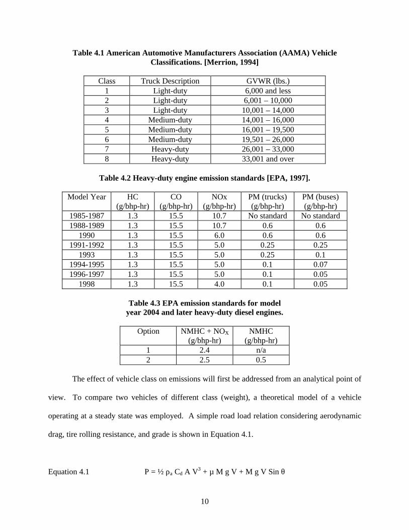
The American Automotive Manufacturers Association (AAMA) classifies trucks from

class 1 (light-duty trucks) to class 8 (heavy-duty trucks). A complete listing of vehicle

classifications can be seen in Table 4.1 [Merrion, 1994]. For heavy-duty vehicles, emission

regulations are imposed on the engine regardless of the size or specific use of the vehicle in

which the engine may be installed. The FTP transient test used to establish certification to

emissions standards is based upon maximum power, unlike in light-duty applications where the

test uses a chassis dynamometer and is affected by road-load power and vehicle weight. Some

class 1 and 2 trucks may be emissions certified using the light-duty automotive approach

(GVWR < 8500 lbs.). Table 4.2 shows the emission standards for heavy-duty engines from 1985

to 1998. Table 4.3 shows the emission standards for model year 2004 and later heavy-duty

diesel engines. Either option of combined non-methane hydrocarbons (NMHC) and NOX can be

used. The standards for CO and PM in 2004 have not been changed from previous years.

Following an investigation in 1998, selected heavy-duty diesel engine manufacturers were

subject to a consent decree by the EPA requiring the 2004 emissions standards to be met in 2002.

Other penalties to the manufacturers were part of this ruling.

10

Table 4.1 American Automotive Manufacturers Association (AAMA) VehicleClassifications. [Merrion, 1994]

Class Truck Description GVWR (lbs.)1 Light-duty 6,000 and less2 Light-duty 6,001 – 10,0003 Light-duty 10,001 – 14,0004 Medium-duty 14,001 – 16,0005 Medium-duty 16,001 – 19,5006 Medium-duty 19,501 – 26,0007 Heavy-duty 26,001 – 33,0008 Heavy-duty 33,001 and over

Table 4.2 Heavy-duty engine emission standards [EPA, 1997].

Model Year HC(g/bhp-hr)

CO(g/bhp-hr)

NOx(g/bhp-hr)

PM (trucks)(g/bhp-hr)

PM (buses)(g/bhp-hr)

1985-1987 1.3 15.5 10.7 No standard No standard1988-1989 1.3 15.5 10.7 0.6 0.6

1990 1.3 15.5 6.0 0.6 0.61991-1992 1.3 15.5 5.0 0.25 0.25

1993 1.3 15.5 5.0 0.25 0.11994-1995 1.3 15.5 5.0 0.1 0.071996-1997 1.3 15.5 5.0 0.1 0.05

1998 1.3 15.5 4.0 0.1 0.05

Table 4.3 EPA emission standards for modelyear 2004 and later heavy-duty diesel engines.

Option NMHC + NOX

(g/bhp-hr)NMHC

(g/bhp-hr)1 2.4 n/a2 2.5 0.5

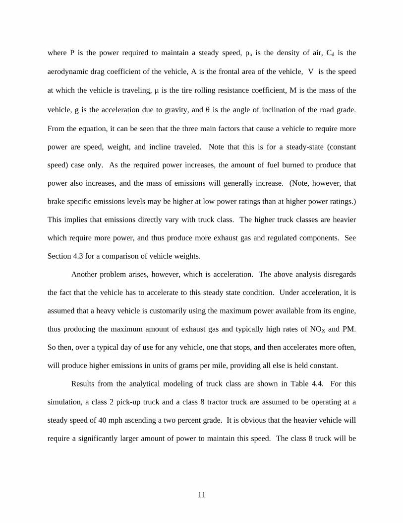
The effect of vehicle class on emissions will first be addressed from an analytical point of

view. To compare two vehicles of different class (weight), a theoretical model of a vehicle

operating at a steady state was employed. A simple road load relation considering aerodynamic

drag, tire rolling resistance, and grade is shown in Equation 4.1.

Equation 4.1 P = ½ ρa Cd A V3 + µ M g V + M g V Sin θ

11

where P is the power required to maintain a steady speed, ρa is the density of air, Cd is the

aerodynamic drag coefficient of the vehicle, A is the frontal area of the vehicle, V is the speed

at which the vehicle is traveling, µ is the tire rolling resistance coefficient, M is the mass of the

vehicle, g is the acceleration due to gravity, and θ is the angle of inclination of the road grade.

From the equation, it can be seen that the three main factors that cause a vehicle to require more

power are speed, weight, and incline traveled. Note that this is for a steady-state (constant

speed) case only. As the required power increases, the amount of fuel burned to produce that

power also increases, and the mass of emissions will generally increase. (Note, however, that

brake specific emissions levels may be higher at low power ratings than at higher power ratings.)

This implies that emissions directly vary with truck class. The higher truck classes are heavier

which require more power, and thus produce more exhaust gas and regulated components. See

Section 4.3 for a comparison of vehicle weights.

Another problem arises, however, which is acceleration. The above analysis disregards

the fact that the vehicle has to accelerate to this steady state condition. Under acceleration, it is

assumed that a heavy vehicle is customarily using the maximum power available from its engine,

thus producing the maximum amount of exhaust gas and typically high rates of NOX and PM.

So then, over a typical day of use for any vehicle, one that stops, and then accelerates more often,

will produce higher emissions in units of grams per mile, providing all else is held constant.

Results from the analytical modeling of truck class are shown in Table 4.4. For this

simulation, a class 2 pick-up truck and a class 8 tractor truck are assumed to be operating at a

steady speed of 40 mph ascending a two percent grade. It is obvious that the heavier vehicle will

require a significantly larger amount of power to maintain this speed. The class 8 truck will be

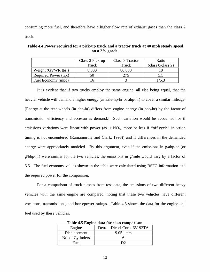
12

consuming more fuel, and therefore have a higher flow rate of exhaust gases than the class 2

truck.

Table 4.4 Power required for a pick-up truck and a tractor truck at 40 mph steady speedon a 2% grade.

Class 2 Pick-upTruck

Class 8 TractorTruck

Ratio(class 8/class 2)

Weight (GVWR lbs.) 8,000 80,000 10Required Power (hp.) 50 275 5.5Fuel Economy (mpg) 16 3 1/5.3

It is evident that if two trucks employ the same engine, all else being equal, that the

heavier vehicle will demand a higher energy (as axle-hp-hr or ahp-hr) to cover a similar mileage.

[Energy at the rear wheels (in ahp-hr) differs from engine energy (in bhp-hr) by the factor of

transmission efficiency and accessories demand.] Such variation would be accounted for if

emissions variations were linear with power (as is NOX, more or less if “off-cycle” injection

timing is not encountered (Ramamurthy and Clark, 1998)) and if differences in the demanded

energy were appropriately modeled. By this argument, even if the emissions in g/ahp-hr (or

g/bhp-hr) were similar for the two vehicles, the emissions in g/mile would vary by a factor of

5.5. The fuel economy values shown in the table were calculated using BSFC information and

the required power for the comparison.

For a comparison of truck classes from test data, the emissions of two different heavy

vehicles with the same engine are compared, noting that these two vehicles have different

vocations, transmissions, and horsepower ratings. Table 4.5 shows the data for the engine and

fuel used by these vehicles.

Table 4.5 Engine data for class comparison.Engine Detroit Diesel Corp. 6V-92TA

Displacement 9.05 litersNo. of Cylinders 6

Fuel D2

13

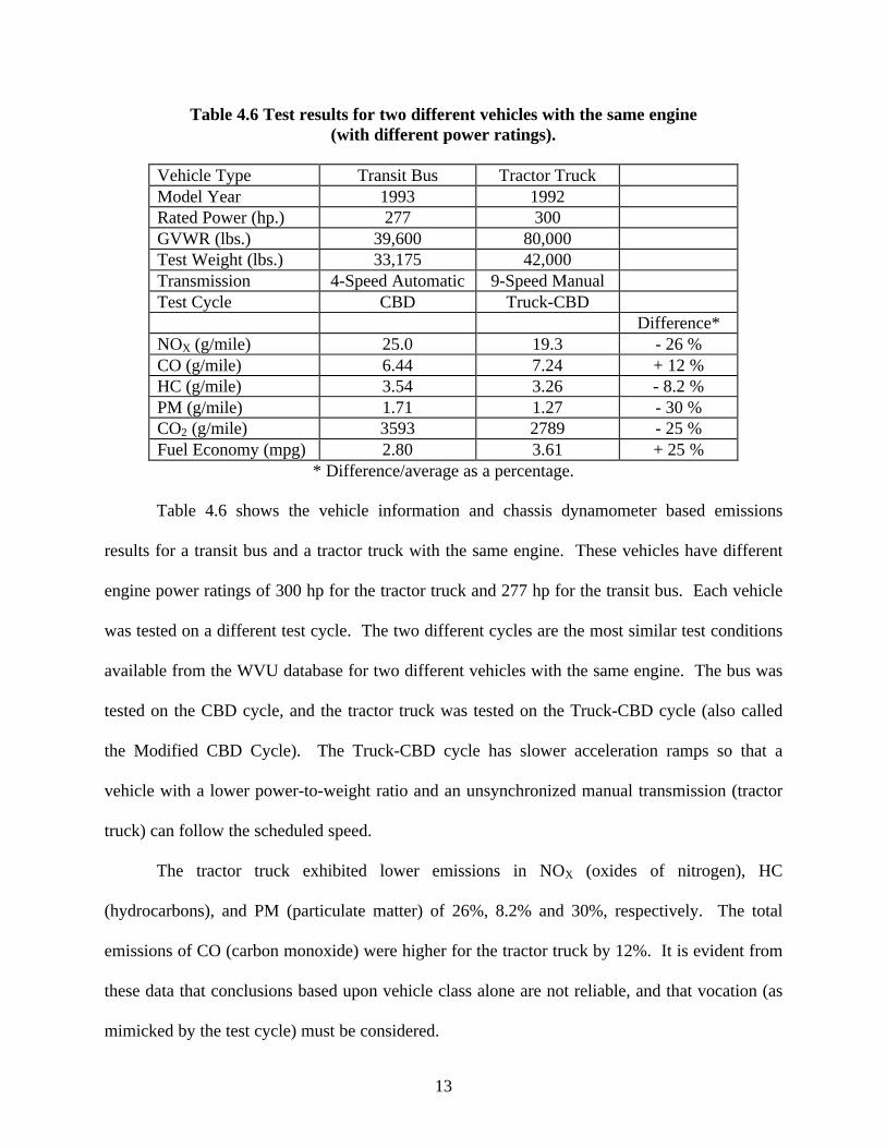
Table 4.6 Test results for two different vehicles with the same engine(with different power ratings).

Vehicle Type Transit Bus Tractor TruckModel Year 1993 1992Rated Power (hp.) 277 300GVWR (lbs.) 39,600 80,000Test Weight (lbs.) 33,175 42,000Transmission 4-Speed Automatic 9-Speed ManualTest Cycle CBD Truck-CBD

Difference*NOX (g/mile) 25.0 19.3 - 26 %CO (g/mile) 6.44 7.24 + 12 %HC (g/mile) 3.54 3.26 - 8.2 %PM (g/mile) 1.71 1.27 - 30 %CO2 (g/mile) 3593 2789 - 25 %Fuel Economy (mpg) 2.80 3.61 + 25 %

* Difference/average as a percentage.

Table 4.6 shows the vehicle information and chassis dynamometer based emissions

results for a transit bus and a tractor truck with the same engine. These vehicles have different

engine power ratings of 300 hp for the tractor truck and 277 hp for the transit bus. Each vehicle

was tested on a different test cycle. The two different cycles are the most similar test conditions

available from the WVU database for two different vehicles with the same engine. The bus was

tested on the CBD cycle, and the tractor truck was tested on the Truck-CBD cycle (also called

the Modified CBD Cycle). The Truck-CBD cycle has slower acceleration ramps so that a

vehicle with a lower power-to-weight ratio and an unsynchronized manual transmission (tractor

truck) can follow the scheduled speed.

The tractor truck exhibited lower emissions in NOX (oxides of nitrogen), HC

(hydrocarbons), and PM (particulate matter) of 26%, 8.2% and 30%, respectively. The total

emissions of CO (carbon monoxide) were higher for the tractor truck by 12%. It is evident from

these data that conclusions based upon vehicle class alone are not reliable, and that vocation (as

mimicked by the test cycle) must be considered.

14

4.2 Driving Test Schedules

4.2.1 Review of Driving Schedules

Driving test schedules are used in the measurement of vehicle emissions with a chassis

dynamometer. The traffic conditions and the routes traveled by each vehicle affect driving

operation. In a similar way, test schedules vary widely in that they attempt to mimic specific

driving behavior. Consequently, measured vehicle emissions are largely affected by the driving

schedule. For comparison, existing test schedules have been divided into two groups for

description below, namely synthesized and actual test schedules. Synthesized schedules are

geometric in nature and usually consist of constant acceleration and constant speed phases. The

actual or realistic driving schedules are derived or created from data collected as a vehicle

performs its tasks. Most chassis test schedules are defined by a speed versus time trace, with

load implied by a road load equation with no gradient assumed. Emissions testing was

conducted on engines for EPA certification and so chassis driving schedules do not play a direct

role in current emissions regulation. The test schedules for engine testing are commonly defined

by speed and torque traces over a period of time [Merrion, 1994]. The actual speeds and torques

are derived using the maximum torque curve and rated and idle speeds of the engine.

Relevant schedules, presented and discussed below, include four synthesized for chassis

testing, two from the engine certification test, three cycles developed from actual truck data, and

three engine test cycles. Speed versus time plots of every test cycle and route discussed were

included for visual comparison.

Synthesized Chassis Schedules

Central Business District

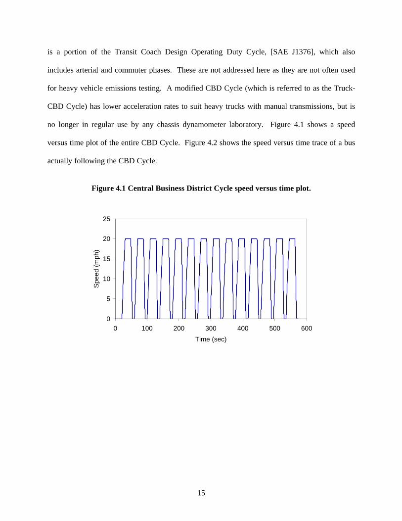
The Central Business District (CBD) cycle is a synthesized driving cycle originally

created for performance verification and fuel economy measurement of transit buses. This cycle

15

is a portion of the Transit Coach Design Operating Duty Cycle, [SAE J1376], which also

includes arterial and commuter phases. These are not addressed here as they are not often used

for heavy vehicle emissions testing. A modified CBD Cycle (which is referred to as the Truck-

CBD Cycle) has lower acceleration rates to suit heavy trucks with manual transmissions, but is

no longer in regular use by any chassis dynamometer laboratory. Figure 4.1 shows a speed

versus time plot of the entire CBD Cycle. Figure 4.2 shows the speed versus time trace of a bus

actually following the CBD Cycle.

Figure 4.1 Central Business District Cycle speed versus time plot.

0

5

10

15

20

25

0 100 200 300 400 500 600

Time (sec)

Spe

ed (

mph

)

16

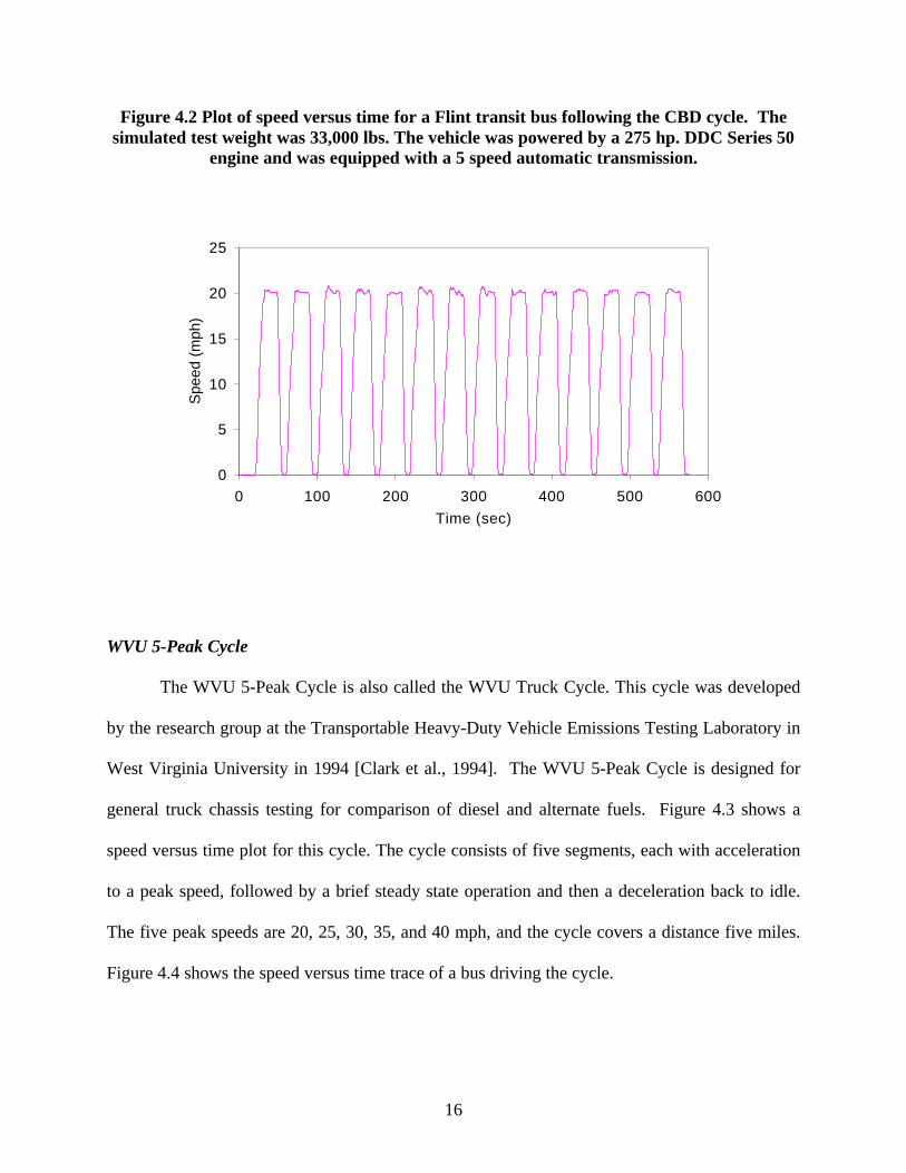
Figure 4.2 Plot of speed versus time for a Flint transit bus following the CBD cycle. Thesimulated test weight was 33,000 lbs. The vehicle was powered by a 275 hp. DDC Series 50

engine and was equipped with a 5 speed automatic transmission.

0

5

10

15

20

25

0 100 200 300 400 500 600

Time (sec)

Spe

ed (

mph

)

WVU 5-Peak Cycle

The WVU 5-Peak Cycle is also called the WVU Truck Cycle. This cycle was developed

by the research group at the Transportable Heavy-Duty Vehicle Emissions Testing Laboratory in

West Virginia University in 1994 [Clark et al., 1994]. The WVU 5-Peak Cycle is designed for

general truck chassis testing for comparison of diesel and alternate fuels. Figure 4.3 shows a

speed versus time plot for this cycle. The cycle consists of five segments, each with acceleration

to a peak speed, followed by a brief steady state operation and then a deceleration back to idle.

The five peak speeds are 20, 25, 30, 35, and 40 mph, and the cycle covers a distance five miles.

Figure 4.4 shows the speed versus time trace of a bus driving the cycle.

17

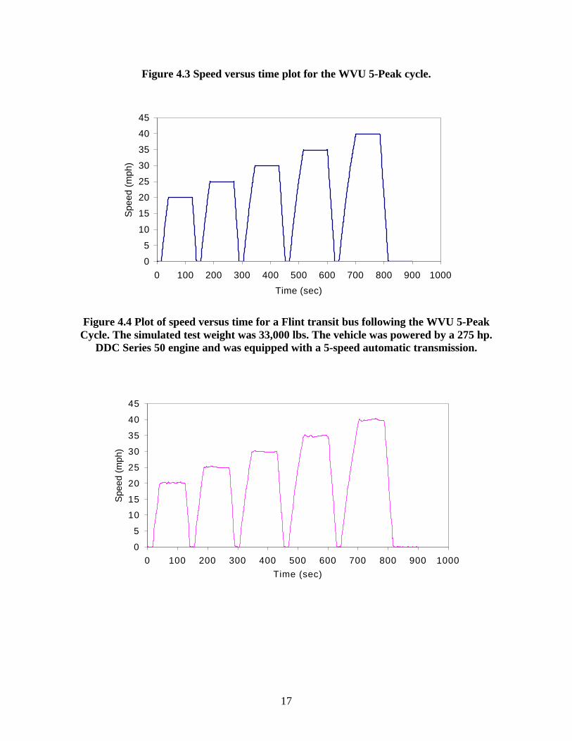
Figure 4.3 Speed versus time plot for the WVU 5-Peak cycle.

0

5

10

15

20

25

30

35

40

45

0 100 200 300 400 500 600 700 800 900 1000

Time (sec)

Spe

ed (

mph

)

Figure 4.4 Plot of speed versus time for a Flint transit bus following the WVU 5-PeakCycle. The simulated test weight was 33,000 lbs. The vehicle was powered by a 275 hp.

DDC Series 50 engine and was equipped with a 5-speed automatic transmission.

0

5

10

15

20

25

30

35

40

45

0 100 200 300 400 500 600 700 800 900 1000

Time (sec)

Spe

ed (

mph

)

18

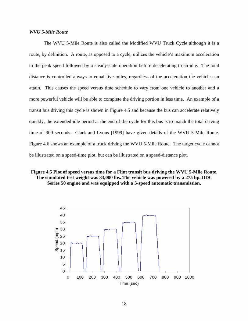
WVU 5-Mile Route

The WVU 5-Mile Route is also called the Modified WVU Truck Cycle although it is a

route, by definition. A route, as opposed to a cycle, utilizes the vehicle’s maximum acceleration

to the peak speed followed by a steady-state operation before decelerating to an idle. The total

distance is controlled always to equal five miles, regardless of the acceleration the vehicle can

attain. This causes the speed versus time schedule to vary from one vehicle to another and a

more powerful vehicle will be able to complete the driving portion in less time. An example of a

transit bus driving this cycle is shown in Figure 4.5 and because the bus can accelerate relatively

quickly, the extended idle period at the end of the cycle for this bus is to match the total driving

time of 900 seconds. Clark and Lyons [1999] have given details of the WVU 5-Mile Route.

Figure 4.6 shows an example of a truck driving the WVU 5-Mile Route. The target cycle cannot

be illustrated on a speed-time plot, but can be illustrated on a speed-distance plot.

Figure 4.5 Plot of speed versus time for a Flint transit bus driving the WVU 5-Mile Route.The simulated test weight was 33,000 lbs. The vehicle was powered by a 275 hp. DDC

Series 50 engine and was equipped with a 5-speed automatic transmission.

0

5

10

15

20

25

30

35

40

45

0 100 200 300 400 500 600 700 800 900 1000

Time (sec)

Spe

ed (

mph

)

19

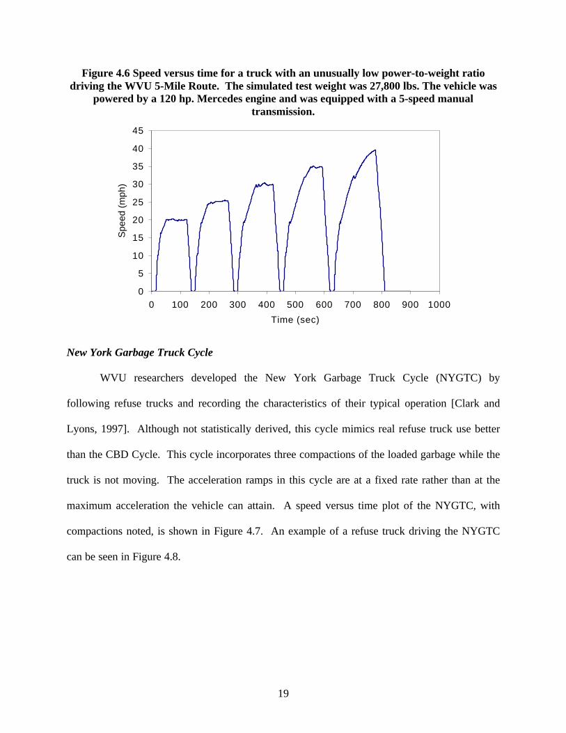
Figure 4.6 Speed versus time for a truck with an unusually low power-to-weight ratiodriving the WVU 5-Mile Route. The simulated test weight was 27,800 lbs. The vehicle was

powered by a 120 hp. Mercedes engine and was equipped with a 5-speed manualtransmission.

0

5

10

15

20

25

30

35

40

45

0 100 200 300 400 500 600 700 800 900 1000

Time (sec)

Spe

ed (

mph

)

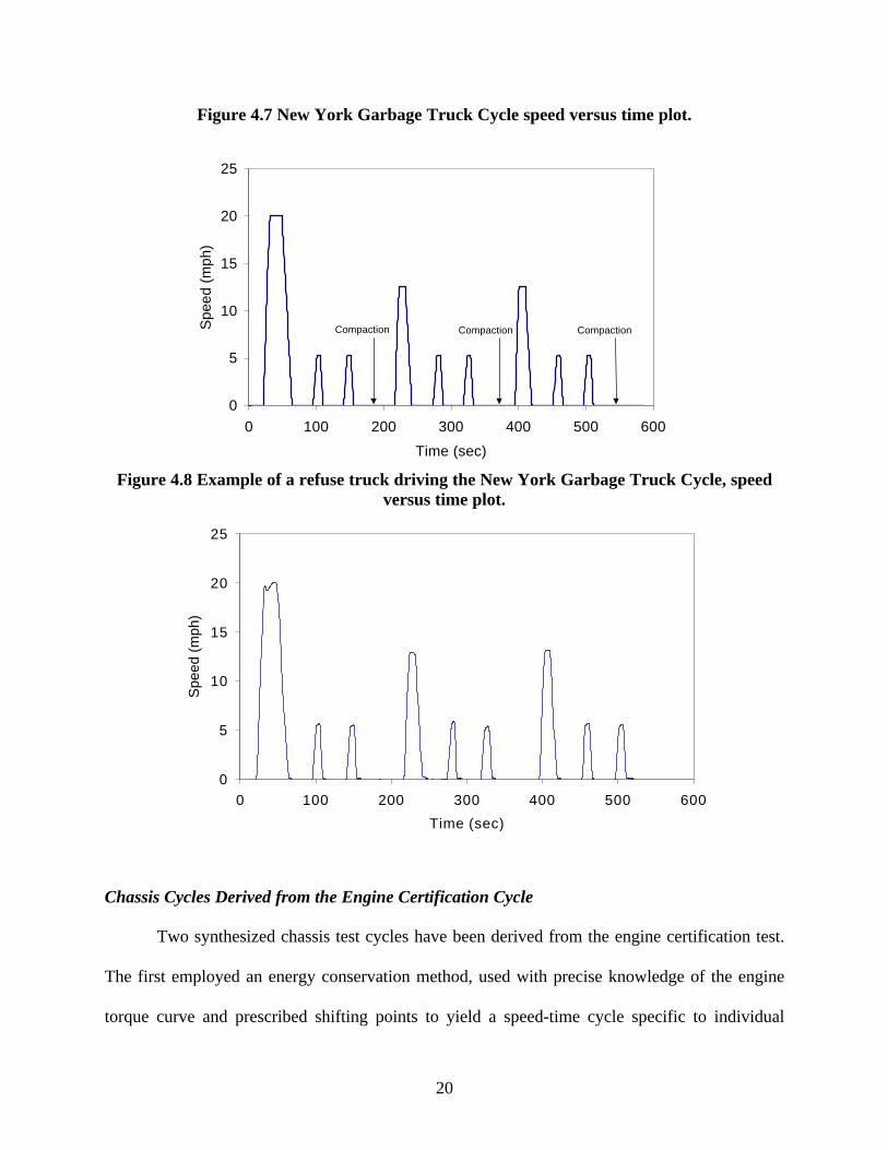
New York Garbage Truck Cycle

WVU researchers developed the New York Garbage Truck Cycle (NYGTC) by

following refuse trucks and recording the characteristics of their typical operation [Clark and

Lyons, 1997]. Although not statistically derived, this cycle mimics real refuse truck use better

than the CBD Cycle. This cycle incorporates three compactions of the loaded garbage while the

truck is not moving. The acceleration ramps in this cycle are at a fixed rate rather than at the

maximum acceleration the vehicle can attain. A speed versus time plot of the NYGTC, with

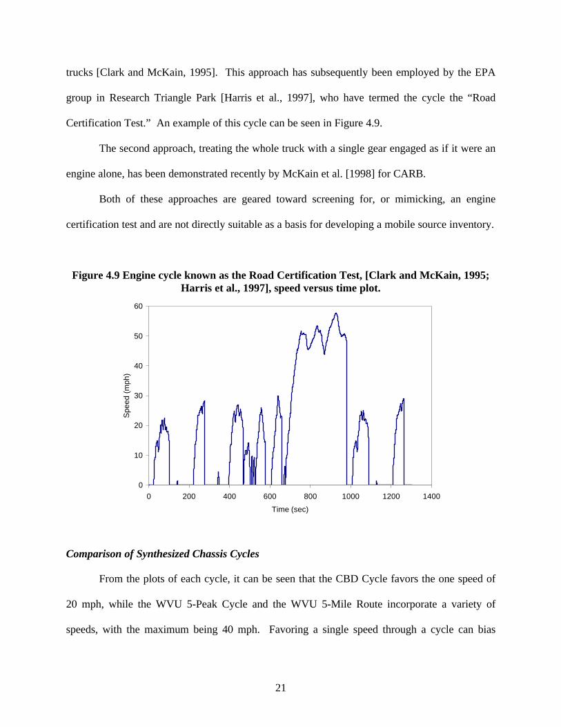
compactions noted, is shown in Figure 4.7. An example of a refuse truck driving the NYGTC

can be seen in Figure 4.8.

20

Figure 4.7 New York Garbage Truck Cycle speed versus time plot.

0

5

10

15

20

25

0 100 200 300 400 500 600

Time (sec)

Spe

ed (

mph

)

Compaction Compaction Compaction

Figure 4.8 Example of a refuse truck driving the New York Garbage Truck Cycle, speedversus time plot.

0

5

10

15

20

25

0 100 200 300 400 500 600

Time (sec)

Spe

ed (

mph

)

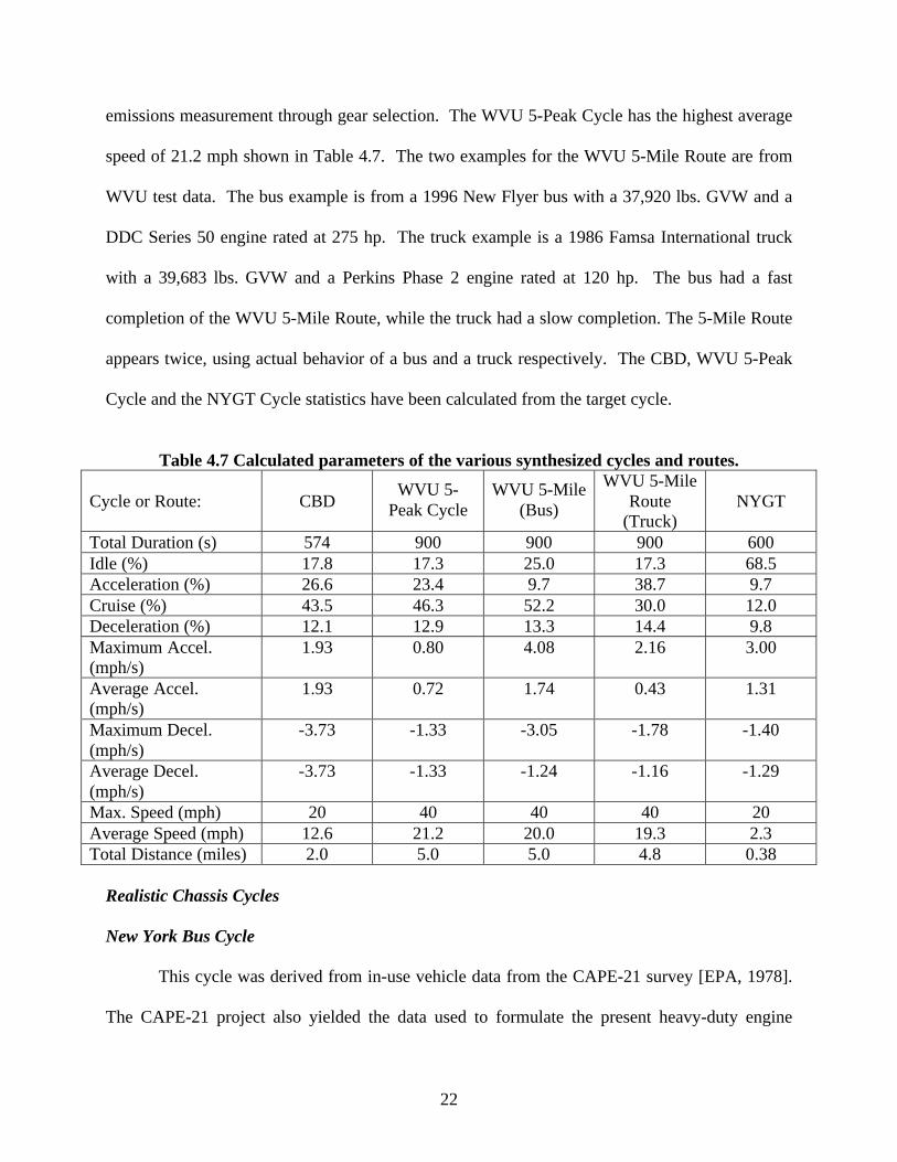
Chassis Cycles Derived from the Engine Certification Cycle

Two synthesized chassis test cycles have been derived from the engine certification test.

The first employed an energy conservation method, used with precise knowledge of the engine

torque curve and prescribed shifting points to yield a speed-time cycle specific to individual

21

trucks [Clark and McKain, 1995]. This approach has subsequently been employed by the EPA

group in Research Triangle Park [Harris et al., 1997], who have termed the cycle the “Road

Certification Test.” An example of this cycle can be seen in Figure 4.9.

The second approach, treating the whole truck with a single gear engaged as if it were an

engine alone, has been demonstrated recently by McKain et al. [1998] for CARB.

Both of these approaches are geared toward screening for, or mimicking, an engine

certification test and are not directly suitable as a basis for developing a mobile source inventory.

Figure 4.9 Engine cycle known as the Road Certification Test, [Clark and McKain, 1995;Harris et al., 1997], speed versus time plot.

0

10

20

30

40

50

60

0 200 400 600 800 1000 1200 1400

Time (sec)

Spe

ed (

mph

)

Comparison of Synthesized Chassis Cycles

From the plots of each cycle, it can be seen that the CBD Cycle favors the one speed of

20 mph, while the WVU 5-Peak Cycle and the WVU 5-Mile Route incorporate a variety of

speeds, with the maximum being 40 mph. Favoring a single speed through a cycle can bias

22

emissions measurement through gear selection. The WVU 5-Peak Cycle has the highest average

speed of 21.2 mph shown in Table 4.7. The two examples for the WVU 5-Mile Route are from

WVU test data. The bus example is from a 1996 New Flyer bus with a 37,920 lbs. GVW and a

DDC Series 50 engine rated at 275 hp. The truck example is a 1986 Famsa International truck

with a 39,683 lbs. GVW and a Perkins Phase 2 engine rated at 120 hp. The bus had a fast

completion of the WVU 5-Mile Route, while the truck had a slow completion. The 5-Mile Route

appears twice, using actual behavior of a bus and a truck respectively. The CBD, WVU 5-Peak

Cycle and the NYGT Cycle statistics have been calculated from the target cycle.

Table 4.7 Calculated parameters of the various synthesized cycles and routes.

Cycle or Route: CBDWVU 5-

Peak CycleWVU 5-Mile

(Bus)

WVU 5-MileRoute

(Truck)NYGT

Total Duration (s) 574 900 900 900 600Idle (%) 17.8 17.3 25.0 17.3 68.5Acceleration (%) 26.6 23.4 9.7 38.7 9.7Cruise (%) 43.5 46.3 52.2 30.0 12.0Deceleration (%) 12.1 12.9 13.3 14.4 9.8Maximum Accel.(mph/s)

1.93 0.80 4.08 2.16 3.00

Average Accel.(mph/s)

1.93 0.72 1.74 0.43 1.31

Maximum Decel.(mph/s)

-3.73 -1.33 -3.05 -1.78 -1.40

Average Decel.(mph/s)

-3.73 -1.33 -1.24 -1.16 -1.29

Max. Speed (mph) 20 40 40 40 20Average Speed (mph) 12.6 21.2 20.0 19.3 2.3Total Distance (miles) 2.0 5.0 5.0 4.8 0.38

Realistic Chassis Cycles

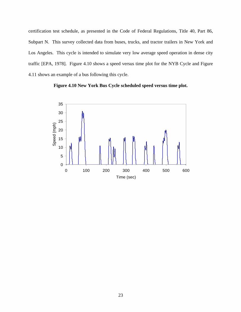
New York Bus Cycle

This cycle was derived from in-use vehicle data from the CAPE-21 survey [EPA, 1978].

The CAPE-21 project also yielded the data used to formulate the present heavy-duty engine

23

certification test schedule, as presented in the Code of Federal Regulations, Title 40, Part 86,

Subpart N. This survey collected data from buses, trucks, and tractor trailers in New York and

Los Angeles. This cycle is intended to simulate very low average speed operation in dense city

traffic [EPA, 1978]. Figure 4.10 shows a speed versus time plot for the NYB Cycle and Figure

4.11 shows an example of a bus following this cycle.

Figure 4.10 New York Bus Cycle scheduled speed versus time plot.

0

5

10

15

20

25

30

35

0 100 200 300 400 500 600

Time (sec)

Spe

ed (

mph

)

24

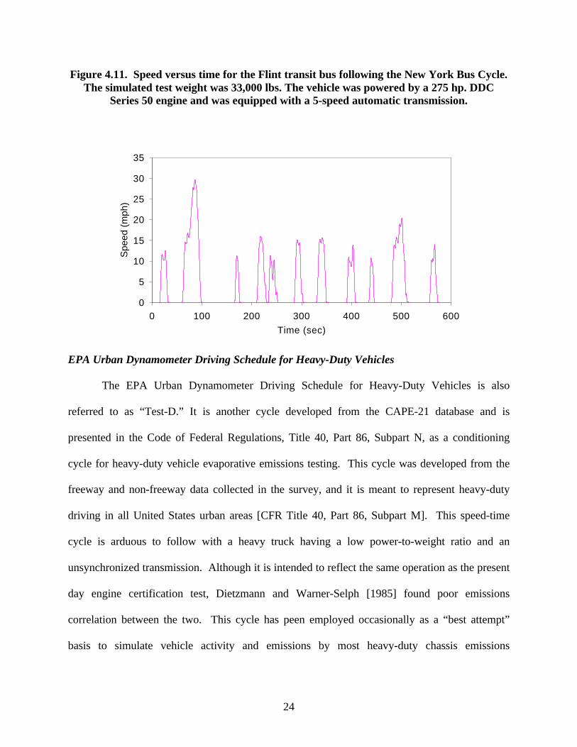
Figure 4.11. Speed versus time for the Flint transit bus following the New York Bus Cycle.The simulated test weight was 33,000 lbs. The vehicle was powered by a 275 hp. DDC

Series 50 engine and was equipped with a 5-speed automatic transmission.

0

5

10

15

20

25

30

35

0 100 200 300 400 500 600

Time (sec)

Spe

ed (

mph

)

EPA Urban Dynamometer Driving Schedule for Heavy-Duty Vehicles

The EPA Urban Dynamometer Driving Schedule for Heavy-Duty Vehicles is also

referred to as “Test-D.” It is another cycle developed from the CAPE-21 database and is

presented in the Code of Federal Regulations, Title 40, Part 86, Subpart N, as a conditioning

cycle for heavy-duty vehicle evaporative emissions testing. This cycle was developed from the

freeway and non-freeway data collected in the survey, and it is meant to represent heavy-duty

driving in all United States urban areas [CFR Title 40, Part 86, Subpart M]. This speed-time

cycle is arduous to follow with a heavy truck having a low power-to-weight ratio and an

unsynchronized transmission. Although it is intended to reflect the same operation as the present

day engine certification test, Dietzmann and Warner-Selph [1985] found poor emissions

correlation between the two. This cycle has peen employed occasionally as a “best attempt”

basis to simulate vehicle activity and emissions by most heavy-duty chassis emissions

25

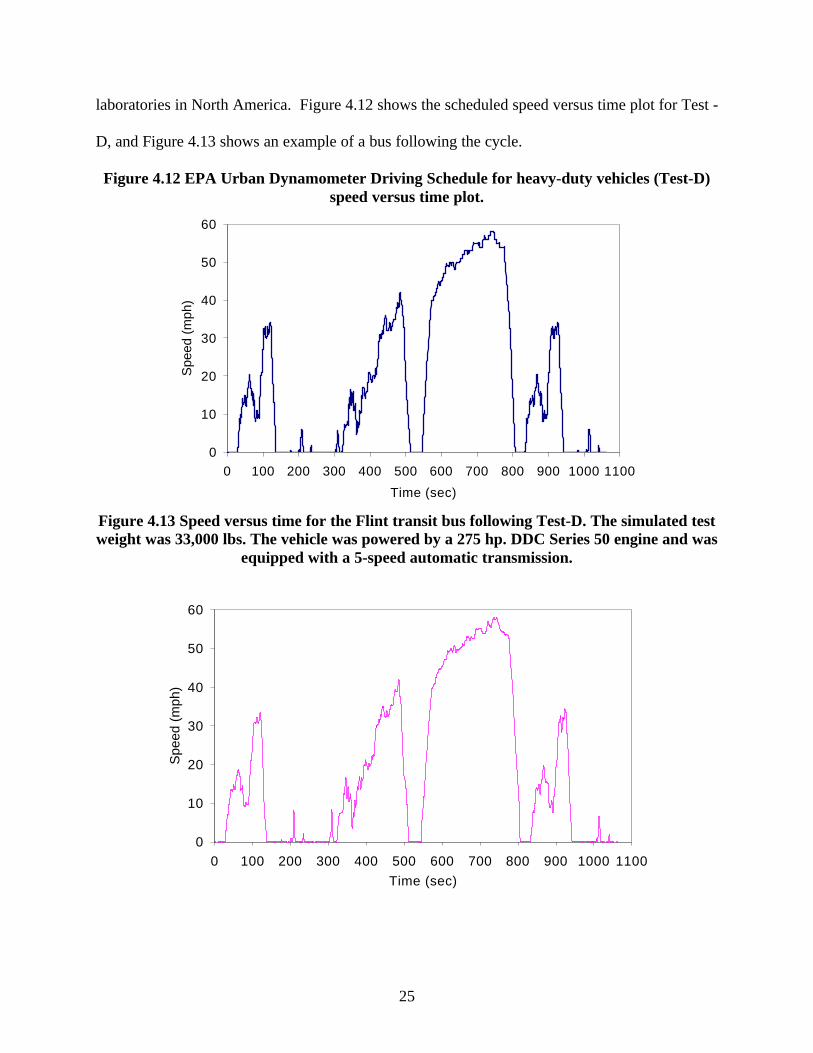
laboratories in North America. Figure 4.12 shows the scheduled speed versus time plot for Test -

D, and Figure 4.13 shows an example of a bus following the cycle.

Figure 4.12 EPA Urban Dynamometer Driving Schedule for heavy-duty vehicles (Test-D)speed versus time plot.

0

10

20

30

40

50

60

0 100 200 300 400 500 600 700 800 900 1000 1100

Time (sec)

Spe

ed (

mph

)

Figure 4.13 Speed versus time for the Flint transit bus following Test-D. The simulated testweight was 33,000 lbs. The vehicle was powered by a 275 hp. DDC Series 50 engine and was

equipped with a 5-speed automatic transmission.

0

10

20

30

40

50

60

0 100 200 300 400 500 600 700 800 900 1000 1100

Time (sec)

Spe

ed (

mph

)

26

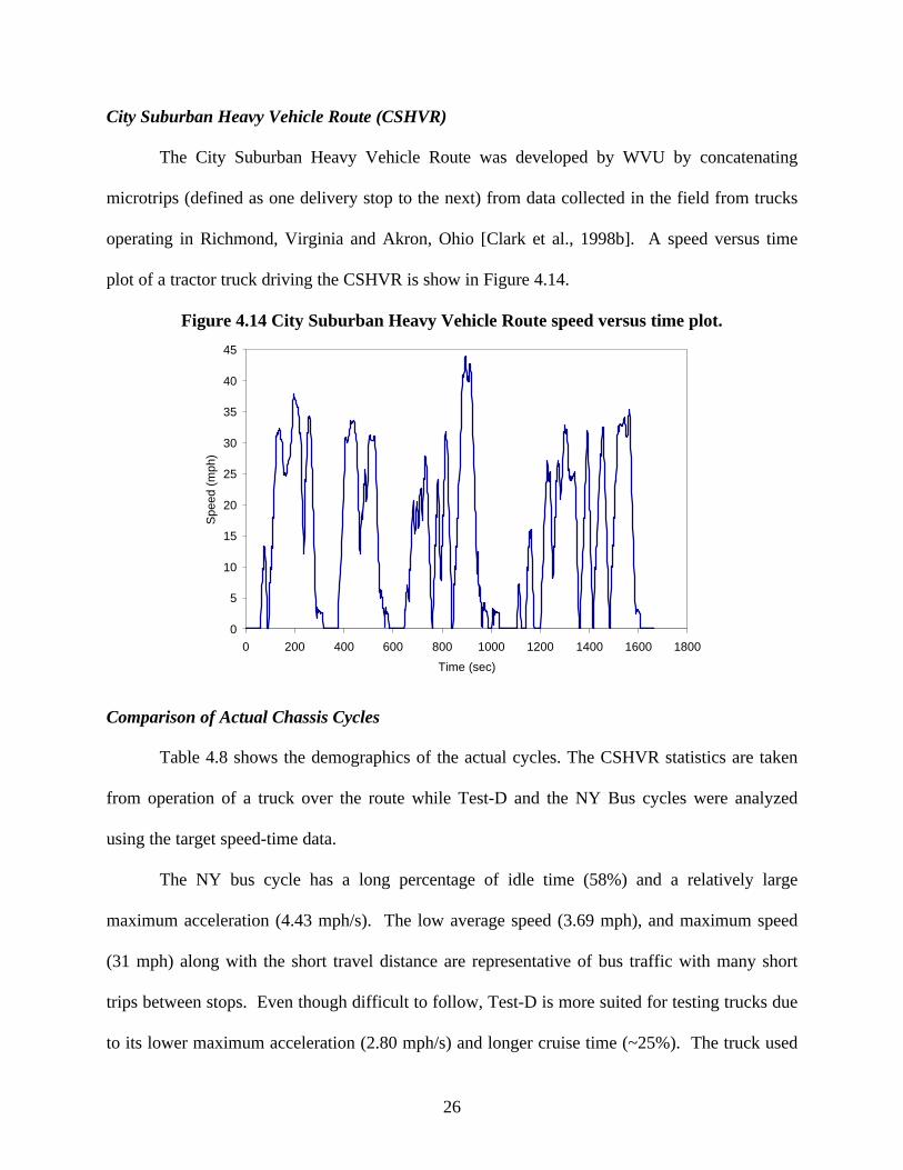
City Suburban Heavy Vehicle Route (CSHVR)

The City Suburban Heavy Vehicle Route was developed by WVU by concatenating

microtrips (defined as one delivery stop to the next) from data collected in the field from trucks

operating in Richmond, Virginia and Akron, Ohio [Clark et al., 1998b]. A speed versus time

plot of a tractor truck driving the CSHVR is show in Figure 4.14.

Figure 4.14 City Suburban Heavy Vehicle Route speed versus time plot.

0

5

10

15

20

25

30

35

40

45

0 200 400 600 800 1000 1200 1400 1600 1800

Time (sec)

Spe

ed (

mph

)

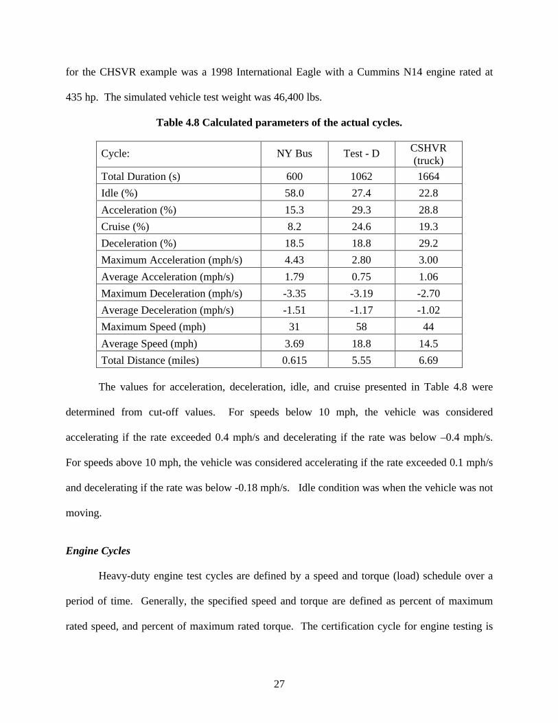
Comparison of Actual Chassis Cycles

Table 4.8 shows the demographics of the actual cycles. The CSHVR statistics are taken

from operation of a truck over the route while Test-D and the NY Bus cycles were analyzed

using the target speed-time data.

The NY bus cycle has a long percentage of idle time (58%) and a relatively large

maximum acceleration (4.43 mph/s). The low average speed (3.69 mph), and maximum speed

(31 mph) along with the short travel distance are representative of bus traffic with many short

trips between stops. Even though difficult to follow, Test-D is more suited for testing trucks due

to its lower maximum acceleration (2.80 mph/s) and longer cruise time (~25%). The truck used

27

for the CHSVR example was a 1998 International Eagle with a Cummins N14 engine rated at

435 hp. The simulated vehicle test weight was 46,400 lbs.

Table 4.8 Calculated parameters of the actual cycles.

Cycle: NY Bus Test - D CSHVR(truck)

Total Duration (s) 600 1062 1664

Idle (%) 58.0 27.4 22.8

Acceleration (%) 15.3 29.3 28.8

Cruise (%) 8.2 24.6 19.3

Deceleration (%) 18.5 18.8 29.2

Maximum Acceleration (mph/s) 4.43 2.80 3.00

Average Acceleration (mph/s) 1.79 0.75 1.06

Maximum Deceleration (mph/s) -3.35 -3.19 -2.70

Average Deceleration (mph/s) -1.51 -1.17 -1.02

Maximum Speed (mph) 31 58 44

Average Speed (mph) 3.69 18.8 14.5

Total Distance (miles) 0.615 5.55 6.69

The values for acceleration, deceleration, idle, and cruise presented in Table 4.8 were

determined from cut-off values. For speeds below 10 mph, the vehicle was considered

accelerating if the rate exceeded 0.4 mph/s and decelerating if the rate was below –0.4 mph/s.

For speeds above 10 mph, the vehicle was considered accelerating if the rate exceeded 0.1 mph/s

and decelerating if the rate was below -0.18 mph/s. Idle condition was when the vehicle was not

moving.

Engine Cycles

Heavy-duty engine test cycles are defined by a speed and torque (load) schedule over a

period of time. Generally, the specified speed and torque are defined as percent of maximum

rated speed, and percent of maximum rated torque. The certification cycle for engine testing is

28

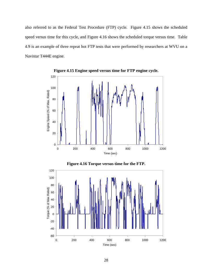
also referred to as the Federal Test Procedure (FTP) cycle. Figure 4.15 shows the scheduled

speed versus time for this cycle, and Figure 4.16 shows the scheduled torque versus time. Table

4.9 is an example of three repeat hot FTP tests that were performed by researchers at WVU on a

Navistar T444E engine.

Figure 4.15 Engine speed versus time for FTP engine cycle.

0

20

40

60

80

100

120

0 200 400 600 800 1000 1200

Time (sec)

Eng

ine

Spe

ed (

% o

f Max

. Rat

ed)

Figure 4.16 Torque versus time for the FTP.

-60

-40

-20

0

20

40

60

80

100

120

0 200 400 600 800 1000 1200

Time (sec)

Tor

que

(% o

f Max

Rat

ed)

29

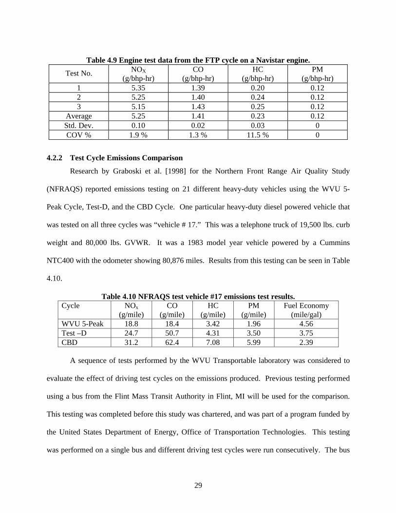
Table 4.9 Engine test data from the FTP cycle on a Navistar engine.

Test No. NOX

(g/bhp-hr)CO

(g/bhp-hr)HC

(g/bhp-hr)PM

(g/bhp-hr)1 5.35 1.39 0.20 0.122 5.25 1.40 0.24 0.123 5.15 1.43 0.25 0.12

Average 5.25 1.41 0.23 0.12Std. Dev. 0.10 0.02 0.03 0COV % 1.9 % 1.3 % 11.5 % 0

4.2.2 Test Cycle Emissions Comparison

Research by Graboski et al. [1998] for the Northern Front Range Air Quality Study

(NFRAQS) reported emissions testing on 21 different heavy-duty vehicles using the WVU 5-

Peak Cycle, Test-D, and the CBD Cycle. One particular heavy-duty diesel powered vehicle that

was tested on all three cycles was “vehicle # 17.” This was a telephone truck of 19,500 lbs. curb

weight and 80,000 lbs. GVWR. It was a 1983 model year vehicle powered by a Cummins

NTC400 with the odometer showing 80,876 miles. Results from this testing can be seen in Table

4.10.

Table 4.10 NFRAQS test vehicle #17 emissions test results.Cycle NOx

(g/mile)CO

(g/mile)HC

(g/mile)PM

(g/mile)Fuel Economy

(mile/gal)WVU 5-Peak 18.8 18.4 3.42 1.96 4.56Test –D 24.7 50.7 4.31 3.50 3.75CBD 31.2 62.4 7.08 5.99 2.39

A sequence of tests performed by the WVU Transportable laboratory was considered to

evaluate the effect of driving test cycles on the emissions produced. Previous testing performed

using a bus from the Flint Mass Transit Authority in Flint, MI will be used for the comparison.

This testing was completed before this study was chartered, and was part of a program funded by

the United States Department of Energy, Office of Transportation Technologies. This testing

was performed on a single bus and different driving test cycles were run consecutively. The bus

30

was outfitted with a Detroit Diesel Series 50 engine coupled to a 5 speed automatic transmission.

The engine was a four-cylinder unit, having 8.5 liters of displacement rated at 275 bhp operating

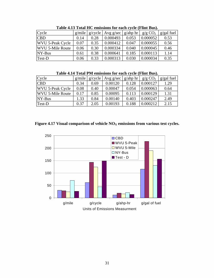
on D2 diesel. Results of this testing are shown in Tables 4.11 through 4.14. Bar graphs of this

data are provided in Figures 4.17 through 4.20. Although this is data from just one bus, many

other similarly equipped busses were tested at this Flint site, and showed consistent bus-to-bus

correlation of emissions data for operation on the CBD Cycle. For the comparison, a range of

emissions parameters was employed to show the difference in emissions based on various

measures (such as miles, cycle, time). In addition to the conventional use of g/mile in chassis

testing, data were also expressed as a total mass per cycle, as an average mass flowrate, as a

mass ratio with CO2 and as grams per gallon of diesel. In addition, since axle speed and torque

were known continuously for each of these tests, it was possible to express the data in mass per

total axle energy delivered, with units of g/axle-hp-hr (or g/ahp-hr). Occurrences of negative

torque during deceleration were not added to the ahp-hr summation.

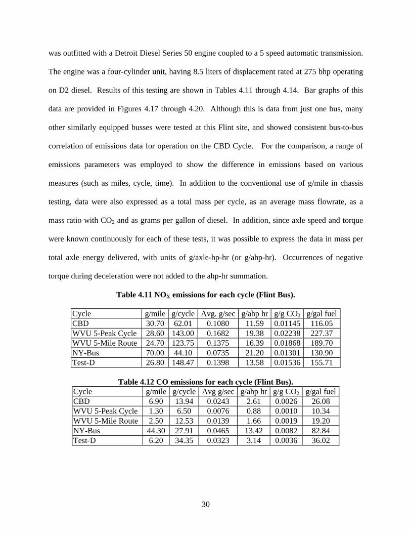
Table 4.11 NOX emissions for each cycle (Flint Bus).

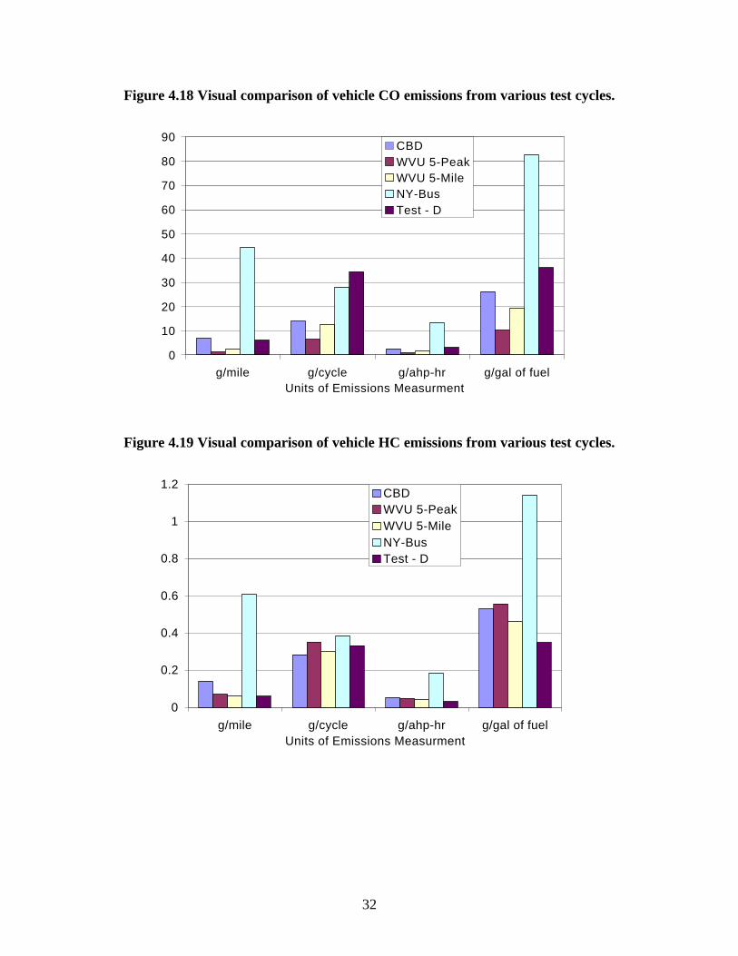
Cycle g/mile g/cycle Avg. g/sec g/ahp hr g/g CO2 g/gal fuelCBD 30.70 62.01 0.1080 11.59 0.01145 116.05WVU 5-Peak Cycle 28.60 143.00 0.1682 19.38 0.02238 227.37WVU 5-Mile Route 24.70 123.75 0.1375 16.39 0.01868 189.70NY-Bus 70.00 44.10 0.0735 21.20 0.01301 130.90Test-D 26.80 148.47 0.1398 13.58 0.01536 155.71

Table 4.12 CO emissions for each cycle (Flint Bus).Cycle g/mile g/cycle Avg g/sec g/ahp hr g/g CO2 g/gal fuelCBD 6.90 13.94 0.0243 2.61 0.0026 26.08WVU 5-Peak Cycle 1.30 6.50 0.0076 0.88 0.0010 10.34WVU 5-Mile Route 2.50 12.53 0.0139 1.66 0.0019 19.20NY-Bus 44.30 27.91 0.0465 13.42 0.0082 82.84Test-D 6.20 34.35 0.0323 3.14 0.0036 36.02

31

Table 4.13 Total HC emissions for each cycle (Flint Bus).Cycle g/mile g/cycle Avg g/sec g/ahp hr g/g CO2 g/gal fuelCBD 0.14 0.28 0.000493 0.053 0.000052 0.53WVU 5-Peak Cycle 0.07 0.35 0.000412 0.047 0.000055 0.56WVU 5-Mile Route 0.06 0.30 0.000334 0.040 0.000045 0.46NY-Bus 0.61 0.38 0.000641 0.185 0.000113 1.14Test-D 0.06 0.33 0.000313 0.030 0.000034 0.35

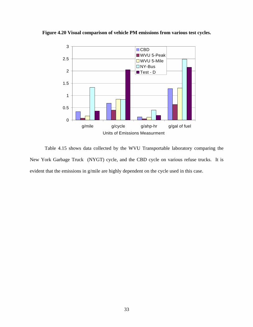
Table 4.14 Total PM emissions for each cycle (Flint Bus).Cycle g/mile g/cycle Avg g/sec g/ahp hr g/g CO2 g/gal fuelCBD 0.34 0.69 0.00120 0.128 0.000127 1.29WVU 5-Peak Cycle 0.08 0.40 0.00047 0.054 0.000063 0.64WVU 5-Mile Route 0.17 0.85 0.00095 0.113 0.000129 1.31NY-Bus 1.33 0.84 0.00140 0.403 0.000247 2.49Test-D 0.37 2.05 0.00193 0.188 0.000212 2.15

Figure 4.17 Visual comparison of vehicle NOX emissions from various test cycles.

0

50

100

150

200

250

g/mile g/cycle g/ahp-hr g/gal of fuel

Units of Emissions Measurment

CBDWVU 5-PeakWVU 5-MileNY-BusTest - D

32

Figure 4.18 Visual comparison of vehicle CO emissions from various test cycles.

0

10

20

30

40

50

60

70

80

90

g/mile g/cycle g/ahp-hr g/gal of fuelUnits of Emissions Measurment


Figure 4.19 Visual comparison of vehicle HC emissions from various test cycles.

0

0.2

0.4

0.6

0.8

1

1.2

g/mile g/cycle g/ahp-hr g/gal of fuelUnits of Emissions Measurment


33

Figure 4.20 Visual comparison of vehicle PM emissions from various test cycles.

0

0.5

1

1.5

2

2.5

3

g/mile g/cycle g/ahp-hr g/gal of fuel

Units of Emissions Measurment


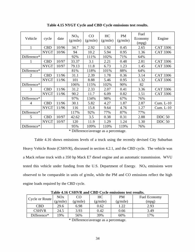
Table 4.15 shows data collected by the WVU Transportable laboratory comparing the

New York Garbage Truck (NYGT) cycle, and the CBD cycle on various refuse trucks. It is

evident that the emissions in g/mile are highly dependent on the cycle used in this case.

34

Table 4.15 NYGT Cycle and CBD Cycle emissions test results.

Vehicle cycle dateNOX

(g/mile)CO

(g/mile)HC

(g/mile)PM

(g/mile)

FuelEconomy

(mpg)Engine

1 CBD 10/96 34.7 2.92 1.92 0.45 2.65 CAT 3306NYGT 10/96 94 10.2 5.94 0.95 1.36 CAT 3306

Difference* 92% 111% 102% 71% 64%1 CBD 10/97 33.37 3.1 2.21 0.48 2.81 CAT 3306

NYGT 10/97 79.13 11.8 6.73 1.23 1.45 CAT 3306Difference* 81% 118% 101% 88% 64%

2 CBD 11/96 31.1 2.39 1.78 0.36 3.14 CAT 3306NYGT 11/96 101 8.88 5.46 0.95 1.32 CAT 3306

Difference* 106% 115% 102% 90% 823 CBD 11/96 31.2 2.33 2.07 0.41 3.36 CAT 3306

NYGT 11/96 90.2 11.7 6.09 0.82 1.51 CAT 3306Difference* 97% 134% 98% 67% 76%

4 CBD 11/96 30.1 5.82 4.27 1.87 2.87 Cum. L-10NYGT 11/96 116 15.8 9.64 4.76 1.27 Cum. L-10

Difference* 117% 92% 77% 87% 77%5 CBD 10/97 42.62 3.5 0.38 0.31 2.88 DDC 50

NYGT 10/97 120 11.9 1.29 1.24 1.30 DDC 50Difference* 95% 109% 110% 119% 76%

* Difference/average as a percentage.

Table 4.16 shows emissions levels of a truck using the recently devised City Suburban

Heavy Vehicle Route (CSHVR), discussed in section 4.2.1, and the CBD cycle. The vehicle was

a Mack refuse truck with a 350 hp Mack E7 diesel engine and an automatic transmission. WVU

tested this vehicle under funding from the U.S. Department of Energy. NOX emissions were

observed to be comparable in units of g/mile, while the PM and CO emissions reflect the high

engine loads required by the CBD cycle.

Table 4.16 CSHVR and CBD Cycle emissions test results.

Cycle or Route NOx(g/mile)

CO(g/mile)

HC(g/mile)

PM(g/mile)

Fuel Economy(mpg)

CBD 29.6 6.98 0.62 1.22 2.93CSHVR 24.5 3.93 0.42 0.66 3.49

Difference* 19% 56% 39% 60% 17%* Difference/average as a percentage.

35

Conclusions from Emissions Data

In Tables 4.11 to 4.14, the emissions in g/g CO2 and g/gal fuel need not be discussed

separately, as they are linked by carbon balance and fuel consumption. In this unit conversion

analysis, the diesel density was taken as 3028 g/gal, diesel carbon-hydrogen ratio was 0.59 and

no mass loss due to blow-by past the rings was assumed.

From the WVU data on the Flint bus, it is evident that the units in which the emissions

are expressed are significant. For example, considering NOX, the NY Bus Cycle is highest of all

the cycles in g/mile, but lowest in average g/sec. This is to be expected due to its low speed and

high idle content. Also, the CBD Cycle and WVU 5-Peak Cycle yield similar emissions in

g/mile, but emissions differing by a factor of two in g/ahp-hr. This is to be expected because the

vital ratios of the cycles, such as ahp-hr/mile, vary widely, as supported by the data in Tables 4.7

and 4.8.

In currency of g/mile, the WVU bus data show that all cycles yield NOX in the range of

24.7 to 30.7 g/mile, with the NY bus cycle an outlier at 70 g/mile. This is because the NY bus

cycle covers a short distance over its duration relative to other cycles. One may conclude that

NOX data, in g/mile, remain fairly consistent for most cycles in current use. For the NFRAQS

telephone truck data, NOX ranged from 18.8 to 31.2 g/mile for the three cycles used, which is a

wider relative variation than for the WVU bus data.

Variations in both CO and PM are acknowledged to be higher than for NOX, all else

being equal. This is borne out by the data of both the NFRAQS and WVU studies. For the

WVU bus, excluding the NY Bus Cycle as an outlier, emissions of CO in g/mile varied by a

factor of three over the four cycles used, and the NFRAQS data yielded a similar ratio. For PM

in both studies the range was a factor of three to four, in g/mile. In the NFRAQS study the ratio

36

of PM in g/mile of the CBD to the WVU 5-Peak Cycle was three, while in the WVU study it was

4.25. One must conclude that the cycle chosen has profound effect on PM and CO levels, if they

are expressed in g/mile. The WVU data showed that choice of units in g/ahp-hr did not improve

cycle-to-cycle agreement by much. This criticizes the present inventory approach of MOBILE

and EMFAC with respect to CO and PM.

Hydrocarbon emissions from diesel engines are customarily low and are of less interest

than NOX and PM emissions. Both the NFRAQS and the WVU data showed cycle-to-cycle

variations of a factor of two, when the units were in g/mile, and when the NY Bus Cycle was

excluded.

Of specific interest is the comparison of the WVU data for the bus using the WVU 5-

Peak Cycle and the WVU 5-Mile Route. Both cycles are similar except that the 5-Peak Cycle

does not demand full power from the bus engine upon acceleration. PM values in g/mile for the

full power operation (route) are slightly more than twice as high as for the cycle. This confirms

the sensitivity of CO and PM emissions to engine loading, in contrast to the relative stability of

the NOX emissions in units of g/mile.

The diesel emissions from the CSHVR testing were lower than the CBD Cycle emissions

in every exhaust gas component in the case of the Mack refuse truck. The fuel economy

produced with the CSHVR was better than that recorded from the CBD Cycle.

The conclusions from Graboski et al. [1998] indicate the trend of the CBD Cycle

producing the highest emissions, and the WVU 5-Peak Cycle producing the lowest emissions

with the Test-D in between them. This trend was attributed to the CBD Cycle being the most

aggressive cycle with more acceleration ramps and more sustained high acceleration than the

other cycles.

37

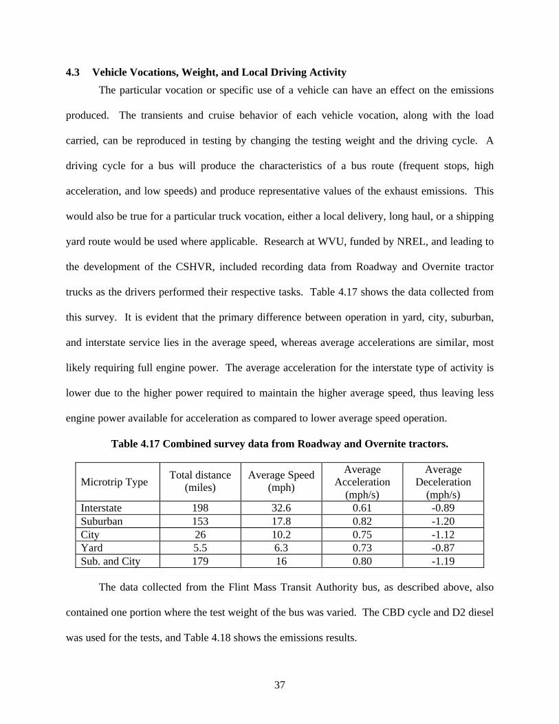
4.3 Vehicle Vocations, Weight, and Local Driving Activity

The particular vocation or specific use of a vehicle can have an effect on the emissions

produced. The transients and cruise behavior of each vehicle vocation, along with the load

carried, can be reproduced in testing by changing the testing weight and the driving cycle. A

driving cycle for a bus will produce the characteristics of a bus route (frequent stops, high

acceleration, and low speeds) and produce representative values of the exhaust emissions. This

would also be true for a particular truck vocation, either a local delivery, long haul, or a shipping

yard route would be used where applicable. Research at WVU, funded by NREL, and leading to

the development of the CSHVR, included recording data from Roadway and Overnite tractor

trucks as the drivers performed their respective tasks. Table 4.17 shows the data collected from

this survey. It is evident that the primary difference between operation in yard, city, suburban,

and interstate service lies in the average speed, whereas average accelerations are similar, most

likely requiring full engine power. The average acceleration for the interstate type of activity is

lower due to the higher power required to maintain the higher average speed, thus leaving less

engine power available for acceleration as compared to lower average speed operation.

Table 4.17 Combined survey data from Roadway and Overnite tractors.

Microtrip TypeTotal distance

(miles)Average Speed

(mph)

AverageAcceleration

(mph/s)

AverageDeceleration

(mph/s)Interstate 198 32.6 0.61 -0.89Suburban 153 17.8 0.82 -1.20City 26 10.2 0.75 -1.12Yard 5.5 6.3 0.73 -0.87Sub. and City 179 16 0.80 -1.19

The data collected from the Flint Mass Transit Authority bus, as described above, also

contained one portion where the test weight of the bus was varied. The CBD cycle and D2 diesel

was used for the tests, and Table 4.18 shows the emissions results.

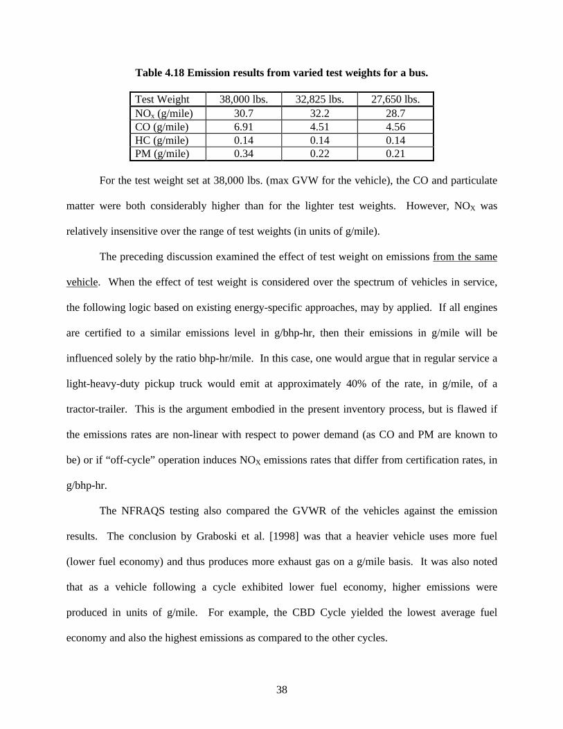
38

Table 4.18 Emission results from varied test weights for a bus.

Test Weight 38,000 lbs. 32,825 lbs. 27,650 lbs.NOx (g/mile) 30.7 32.2 28.7CO (g/mile) 6.91 4.51 4.56HC (g/mile) 0.14 0.14 0.14PM (g/mile) 0.34 0.22 0.21

For the test weight set at 38,000 lbs. (max GVW for the vehicle), the CO and particulate

matter were both considerably higher than for the lighter test weights. However, NOX was

relatively insensitive over the range of test weights (in units of g/mile).

The preceding discussion examined the effect of test weight on emissions from the same

vehicle. When the effect of test weight is considered over the spectrum of vehicles in service,

the following logic based on existing energy-specific approaches, may by applied. If all engines

are certified to a similar emissions level in g/bhp-hr, then their emissions in g/mile will be

influenced solely by the ratio bhp-hr/mile. In this case, one would argue that in regular service a

light-heavy-duty pickup truck would emit at approximately 40% of the rate, in g/mile, of a

tractor-trailer. This is the argument embodied in the present inventory process, but is flawed if

the emissions rates are non-linear with respect to power demand (as CO and PM are known to

be) or if “off-cycle” operation induces NOX emissions rates that differ from certification rates, in

g/bhp-hr.

The NFRAQS testing also compared the GVWR of the vehicles against the emission

results. The conclusion by Graboski et al. [1998] was that a heavier vehicle uses more fuel

(lower fuel economy) and thus produces more exhaust gas on a g/mile basis. It was also noted

that as a vehicle following a cycle exhibited lower fuel economy, higher emissions were

produced in units of g/mile. For example, the CBD Cycle yielded the lowest average fuel

economy and also the highest emissions as compared to the other cycles.

39

The issue of the effect of vehicle vocation is difficult to tackle, but is also covered in part

by the discussion of test cycles above. It is evident that a line haul tractor may be expected to

emit at lower levels in g/mile than an inner-city refuse truck because long idle periods and stop-

and-go operation will increase emissions in g/mile. This is the basis for the development of the

New York Garbage Truck Cycle that has previously been discussed.

Local driving activity also affects heavy vehicle emissions, but is difficult to quantify. A

simple definition of local driving activity would be the differences that occur when a vehicle is

driven or used differently, mainly due to the driving attitudes of different geographic locations.

This is very close to the definition of vehicle vocations, and also impacts the discussion on test

cycles. Local driving habits will also affect the vehicle emissions due to driver-to-driver

variations. The effect that these factors have on vehicle emissions is comparable with different

driving cycles that mimic the particular driving patterns or vehicle uses.

4.4 Fuel Type

Fuels other than conventional diesel provide a means of reducing heavy-duty engine

emissions. Fuels such as compressed natural gas (CNG), liquefied petroleum gas (LPG), and

various alcohols have been used, but require engine modifications for operation. However, using

a reformulated diesel or a diesel equivalent fuel that does not require engine modifications can

produce significant reductions in engine emissions while avoiding the expense of vehicle

modifications. Complete fuel reformulation would affect all heavy-duty diesel vehicles and has

the potential to reduce NOX and PM significantly [Health Effects Institute, 1995]. Diesel fuel

additives have also been used for reduction of emissions as shown by Lange et al. [1997], and

Green et al. [1997]. The most common additive has been a cetane number enhancer. The results

show that a fuel with a higher cetane number ignites earlier and thus uses less fuel to produce the

40

same power. This increase in fuel economy leads to lower emissions and the earlier ignition

generally reduces NOX production during the premix burn.

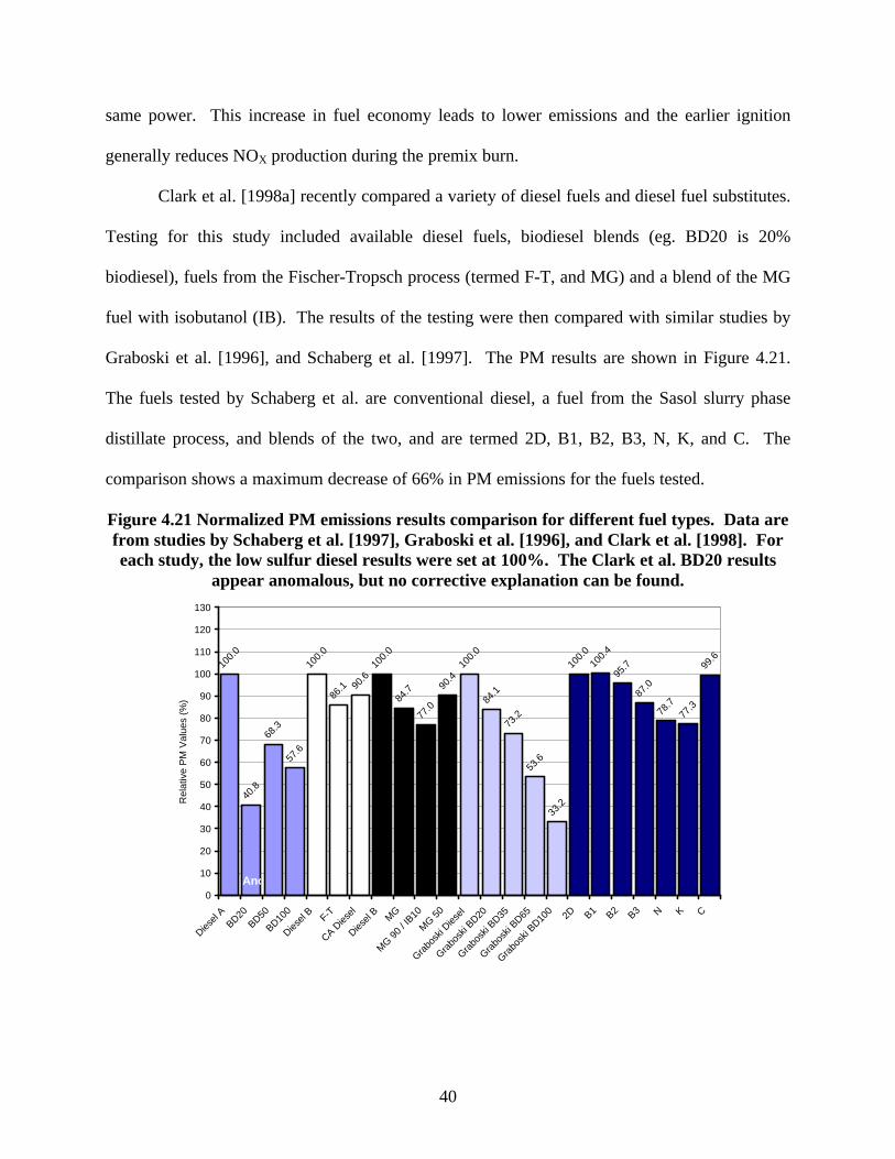
Clark et al. [1998a] recently compared a variety of diesel fuels and diesel fuel substitutes.

Testing for this study included available diesel fuels, biodiesel blends (eg. BD20 is 20%

biodiesel), fuels from the Fischer-Tropsch process (termed F-T, and MG) and a blend of the MG

fuel with isobutanol (IB). The results of the testing were then compared with similar studies by

Graboski et al. [1996], and Schaberg et al. [1997]. The PM results are shown in Figure 4.21.

The fuels tested by Schaberg et al. are conventional diesel, a fuel from the Sasol slurry phase

distillate process, and blends of the two, and are termed 2D, B1, B2, B3, N, K, and C. The

comparison shows a maximum decrease of 66% in PM emissions for the fuels tested.

Figure 4.21 Normalized PM emissions results comparison for different fuel types. Data arefrom studies by Schaberg et al. [1997], Graboski et al. [1996], and Clark et al. [1998]. Foreach study, the low sulfur diesel results were set at 100%. The Clark et al. BD20 results

appear anomalous, but no corrective explanation can be found.

100.

0

40.8

68.3

57.6

100.

0

86.1 90

.610

0.0

84.7

77.0

90.4

100.

0

84.1

73.2

53.6

33.2

100.

010

0.4

95.7

87.0

78.7

77.3

99.6

0

10

20

30

40

50

60

70

80

90

100

110

120

130

Diesel

ABD20

BD50

BD100

Diesel

BF-T

CA Dies

el

Diesel

BM

G

MG 9

0 / I

B10

MG 5

0

Grabo

ski D

iesel

Grabo

ski B

D20

Grabo

ski B

D35

Grabo

ski B

D65

Grabo

ski B

D100 2D B1 B2 B3 N K C

Rel

ativ

e P

M V

alue

s (%

)

Anomaly

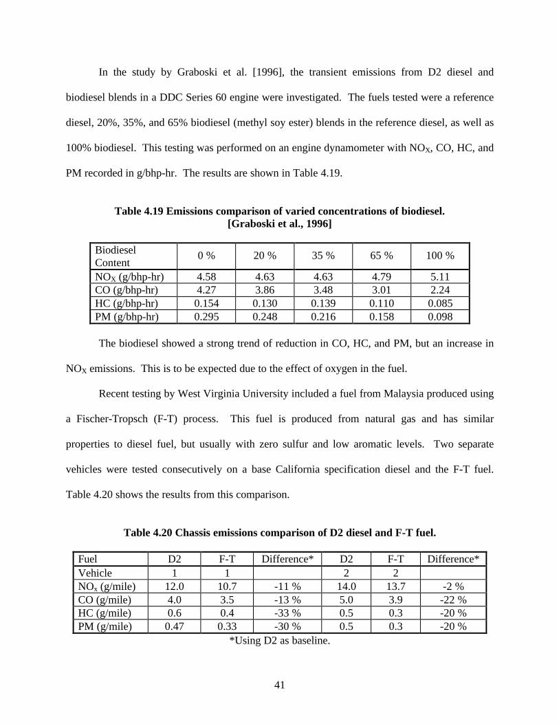
41

In the study by Graboski et al. [1996], the transient emissions from D2 diesel and

biodiesel blends in a DDC Series 60 engine were investigated. The fuels tested were a reference

diesel, 20%, 35%, and 65% biodiesel (methyl soy ester) blends in the reference diesel, as well as

100% biodiesel. This testing was performed on an engine dynamometer with NOX, CO, HC, and

PM recorded in g/bhp-hr. The results are shown in Table 4.19.

Table 4.19 Emissions comparison of varied concentrations of biodiesel.[Graboski et al., 1996]

BiodieselContent

0 % 20 % 35 % 65 % 100 %

NOX (g/bhp-hr) 4.58 4.63 4.63 4.79 5.11CO (g/bhp-hr) 4.27 3.86 3.48 3.01 2.24HC (g/bhp-hr) 0.154 0.130 0.139 0.110 0.085PM (g/bhp-hr) 0.295 0.248 0.216 0.158 0.098

The biodiesel showed a strong trend of reduction in CO, HC, and PM, but an increase in

NOX emissions. This is to be expected due to the effect of oxygen in the fuel.

Recent testing by West Virginia University included a fuel from Malaysia produced using

a Fischer-Tropsch (F-T) process. This fuel is produced from natural gas and has similar

properties to diesel fuel, but usually with zero sulfur and low aromatic levels. Two separate

vehicles were tested consecutively on a base California specification diesel and the F-T fuel.

Table 4.20 shows the results from this comparison.

Table 4.20 Chassis emissions comparison of D2 diesel and F-T fuel.

Fuel D2 F-T Difference* D2 F-T Difference*Vehicle 1 1 2 2NOx (g/mile) 12.0 10.7 -11 % 14.0 13.7 -2 %CO (g/mile) 4.0 3.5 -13 % 5.0 3.9 -22 %HC (g/mile) 0.6 0.4 -33 % 0.5 0.3 -20 %PM (g/mile) 0.47 0.33 -30 % 0.5 0.3 -20 %

*Using D2 as baseline.

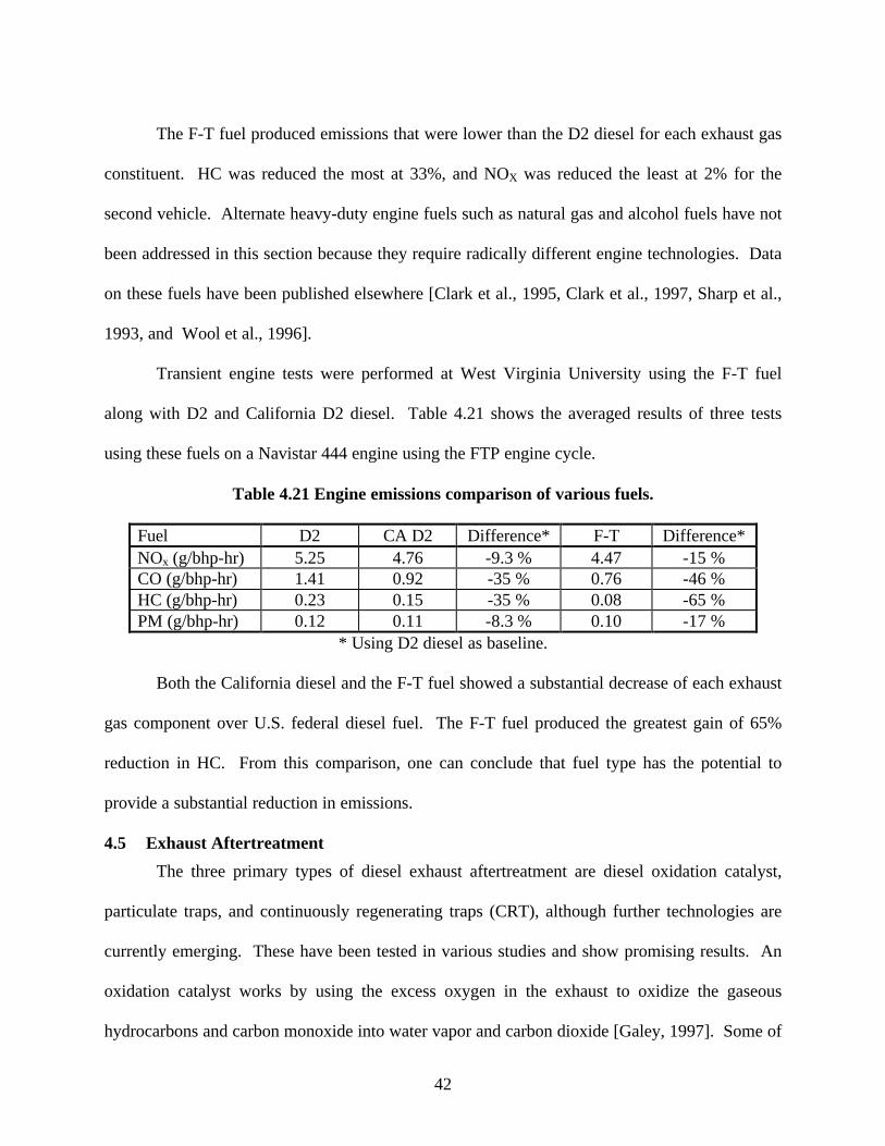
42

The F-T fuel produced emissions that were lower than the D2 diesel for each exhaust gas

constituent. HC was reduced the most at 33%, and NOX was reduced the least at 2% for the

second vehicle. Alternate heavy-duty engine fuels such as natural gas and alcohol fuels have not

been addressed in this section because they require radically different engine technologies. Data

on these fuels have been published elsewhere [Clark et al., 1995, Clark et al., 1997, Sharp et al.,

1993, and Wool et al., 1996].

Transient engine tests were performed at West Virginia University using the F-T fuel

along with D2 and California D2 diesel. Table 4.21 shows the averaged results of three tests

using these fuels on a Navistar 444 engine using the FTP engine cycle.

Table 4.21 Engine emissions comparison of various fuels.

Fuel D2 CA D2 Difference* F-T Difference*NOx (g/bhp-hr) 5.25 4.76 -9.3 % 4.47 -15 %CO (g/bhp-hr) 1.41 0.92 -35 % 0.76 -46 %HC (g/bhp-hr) 0.23 0.15 -35 % 0.08 -65 %PM (g/bhp-hr) 0.12 0.11 -8.3 % 0.10 -17 %

* Using D2 diesel as baseline.

Both the California diesel and the F-T fuel showed a substantial decrease of each exhaust

gas component over U.S. federal diesel fuel. The F-T fuel produced the greatest gain of 65%

reduction in HC. From this comparison, one can conclude that fuel type has the potential to

provide a substantial reduction in emissions.

4.5 Exhaust Aftertreatment

The three primary types of diesel exhaust aftertreatment are diesel oxidation catalyst,

particulate traps, and continuously regenerating traps (CRT), although further technologies are

currently emerging. These have been tested in various studies and show promising results. An

oxidation catalyst works by using the excess oxygen in the exhaust to oxidize the gaseous

hydrocarbons and carbon monoxide into water vapor and carbon dioxide [Galey, 1997]. Some of

43

the soluble organic fraction (SOF) of the PM will also be eliminated. While this type of

aftertreatment is effective in reducing HC, and CO, these are not the specific diesel exhaust

pollutants that are desirable to eliminate. The quest for a NOX reduction catalyst for diesel

engines remains an unattained grail.

A particulate trap is a device where the PM is collected or filtered out of the exhaust and

is regenerated by some external means. This is usually accomplished by either heating the trap

to burn the PM, or using a fuel additive that causes regeneration or having a catalytic substrate

on the filter. These are sometimes not effective in regenerating at low loads and low exhaust

temperatures [Bach et al., 1998].

The most recent type of exhaust aftertreatment developed is the CRT. This type of

system combines an oxidation catalyst and a particulate trap filter that reduces both gaseous and

particulate emissions. The exhaust gases first pass through the catalyst to oxidize CO and HC,

and also convert the majority of NOX to NO2 which is then used to oxidize the PM in the

particulate trap [Galey, 1997]. This aftertreatment method continuously regenerates with no fuel

additives or heater control system. A drawback of this system is that it requires low sulfur

diesel, as sulfur inhibits the catalytic reactions in the system. Reductions with this system are as

high as 90% for CO, HC, and PM, and 15% for NOX [Galey, 1997].

The WVU Transportable Laboratory has performed testing on vehicles with and without

catalytic converters. A particular test was a refuse truck tested in 1995 with an early technology

catalytic converter manufactured by Donaldson. The vehicle was a 1992 model year with 56,515

miles on a Cummins LTA-10 engine supplying power through a 4-speed automatic transmission.

This engine was rated at 260 hp operating on D2 diesel. The testing used the WVU 5-Peak cycle

and Table 4.22 shows the results of this comparison.

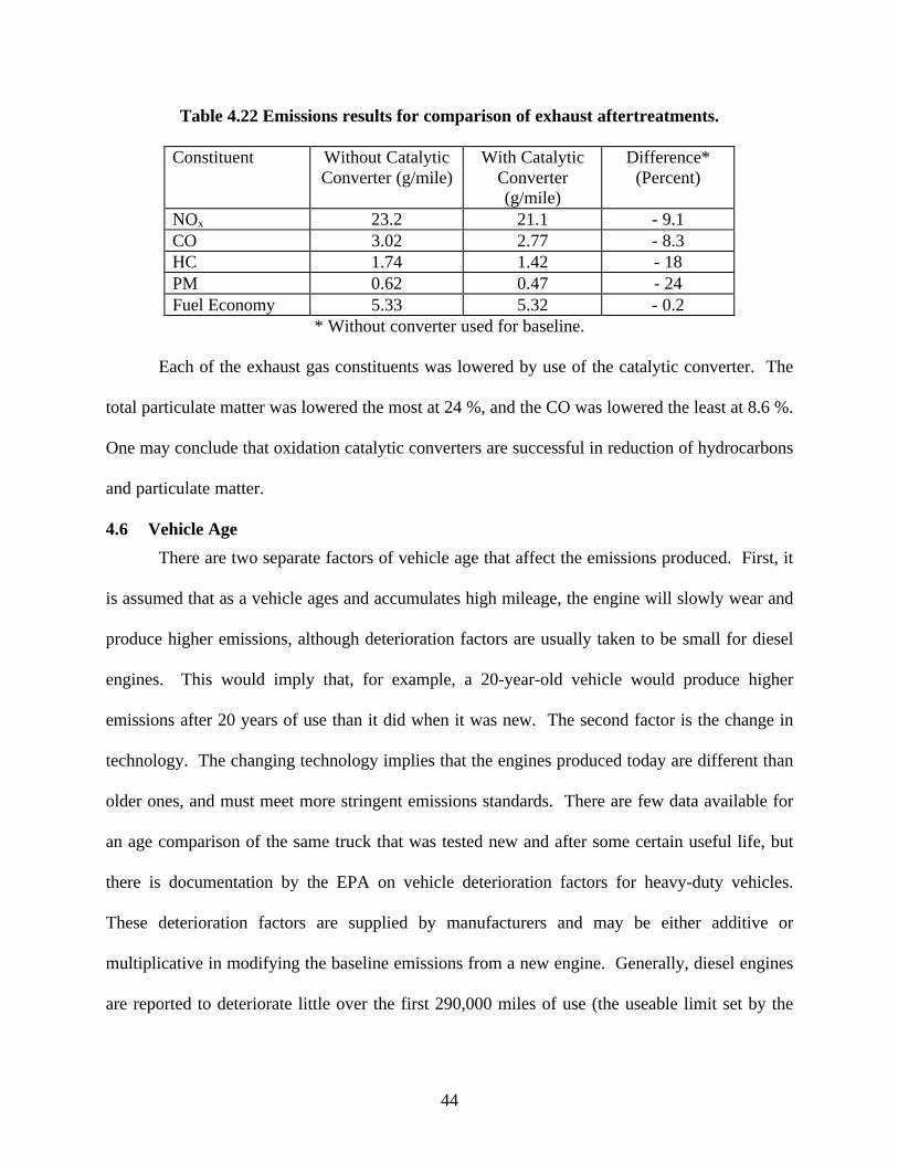
44

Table 4.22 Emissions results for comparison of exhaust aftertreatments.

Constituent Without CatalyticConverter (g/mile)

With CatalyticConverter(g/mile)

Difference*(Percent)

NOx 23.2 21.1 - 9.1CO 3.02 2.77 - 8.3HC 1.74 1.42 - 18PM 0.62 0.47 - 24Fuel Economy 5.33 5.32 - 0.2

* Without converter used for baseline.

Each of the exhaust gas constituents was lowered by use of the catalytic converter. The

total particulate matter was lowered the most at 24 %, and the CO was lowered the least at 8.6 %.

One may conclude that oxidation catalytic converters are successful in reduction of hydrocarbons

and particulate matter.

4.6 Vehicle Age

There are two separate factors of vehicle age that affect the emissions produced. First, it

is assumed that as a vehicle ages and accumulates high mileage, the engine will slowly wear and

produce higher emissions, although deterioration factors are usually taken to be small for diesel

engines. This would imply that, for example, a 20-year-old vehicle would produce higher

emissions after 20 years of use than it did when it was new. The second factor is the change in

technology. The changing technology implies that the engines produced today are different than

older ones, and must meet more stringent emissions standards. There are few data available for

an age comparison of the same truck that was tested new and after some certain useful life, but

there is documentation by the EPA on vehicle deterioration factors for heavy-duty vehicles.

These deterioration factors are supplied by manufacturers and may be either additive or

multiplicative in modifying the baseline emissions from a new engine. Generally, diesel engines

are reported to deteriorate little over the first 290,000 miles of use (the useable limit set by the

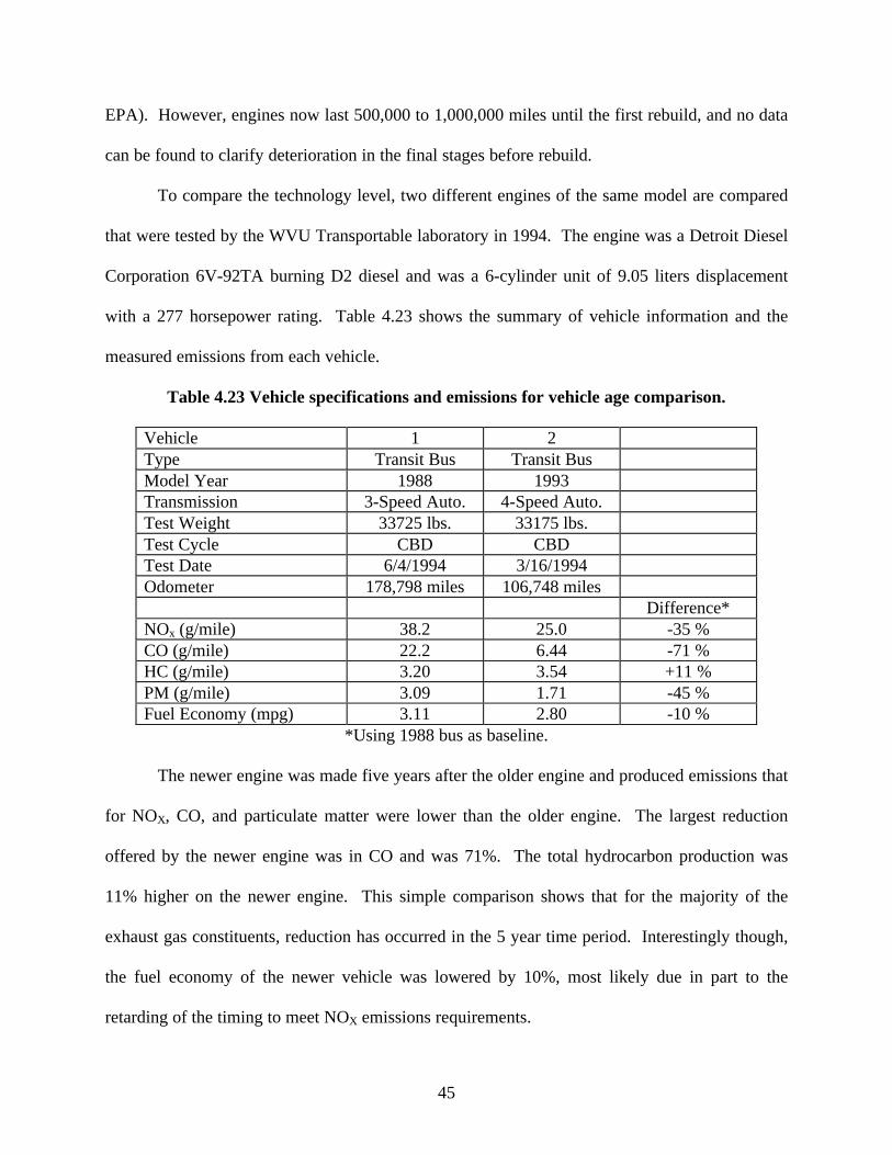
45

EPA). However, engines now last 500,000 to 1,000,000 miles until the first rebuild, and no data

can be found to clarify deterioration in the final stages before rebuild.

To compare the technology level, two different engines of the same model are compared

that were tested by the WVU Transportable laboratory in 1994. The engine was a Detroit Diesel

Corporation 6V-92TA burning D2 diesel and was a 6-cylinder unit of 9.05 liters displacement

with a 277 horsepower rating. Table 4.23 shows the summary of vehicle information and the

measured emissions from each vehicle.

Table 4.23 Vehicle specifications and emissions for vehicle age comparison.

Vehicle 1 2Type Transit Bus Transit BusModel Year 1988 1993Transmission 3-Speed Auto. 4-Speed Auto.Test Weight 33725 lbs. 33175 lbs.Test Cycle CBD CBDTest Date 6/4/1994 3/16/1994Odometer 178,798 miles 106,748 miles

Difference*NOx (g/mile) 38.2 25.0 -35 %CO (g/mile) 22.2 6.44 -71 %HC (g/mile) 3.20 3.54 +11 %PM (g/mile) 3.09 1.71 -45 %Fuel Economy (mpg) 3.11 2.80 -10 %

*Using 1988 bus as baseline.

The newer engine was made five years after the older engine and produced emissions that

for NOX, CO, and particulate matter were lower than the older engine. The largest reduction

offered by the newer engine was in CO and was 71%. The total hydrocarbon production was

11% higher on the newer engine. This simple comparison shows that for the majority of the

exhaust gas constituents, reduction has occurred in the 5 year time period. Interestingly though,

the fuel economy of the newer vehicle was lowered by 10%, most likely due in part to the

retarding of the timing to meet NOX emissions requirements.

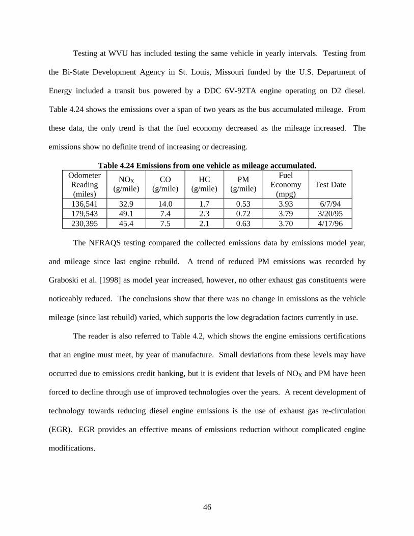
46

Testing at WVU has included testing the same vehicle in yearly intervals. Testing from

the Bi-State Development Agency in St. Louis, Missouri funded by the U.S. Department of

Energy included a transit bus powered by a DDC 6V-92TA engine operating on D2 diesel.

Table 4.24 shows the emissions over a span of two years as the bus accumulated mileage. From

these data, the only trend is that the fuel economy decreased as the mileage increased. The

emissions show no definite trend of increasing or decreasing.

Table 4.24 Emissions from one vehicle as mileage accumulated.OdometerReading(miles)

NOX

(g/mile)CO

(g/mile)HC

(g/mile)PM

(g/mile)

FuelEconomy

(mpg)Test Date

136,541 32.9 14.0 1.7 0.53 3.93 6/7/94179,543 49.1 7.4 2.3 0.72 3.79 3/20/95230,395 45.4 7.5 2.1 0.63 3.70 4/17/96

The NFRAQS testing compared the collected emissions data by emissions model year,

and mileage since last engine rebuild. A trend of reduced PM emissions was recorded by

Graboski et al. [1998] as model year increased, however, no other exhaust gas constituents were

noticeably reduced. The conclusions show that there was no change in emissions as the vehicle

mileage (since last rebuild) varied, which supports the low degradation factors currently in use.

The reader is also referred to Table 4.2, which shows the engine emissions certifications

that an engine must meet, by year of manufacture. Small deviations from these levels may have

occurred due to emissions credit banking, but it is evident that levels of NOX and PM have been

forced to decline through use of improved technologies over the years. A recent development of

technology towards reducing diesel engine emissions is the use of exhaust gas re-circulation

(EGR). EGR provides an effective means of emissions reduction without complicated engine

modifications.

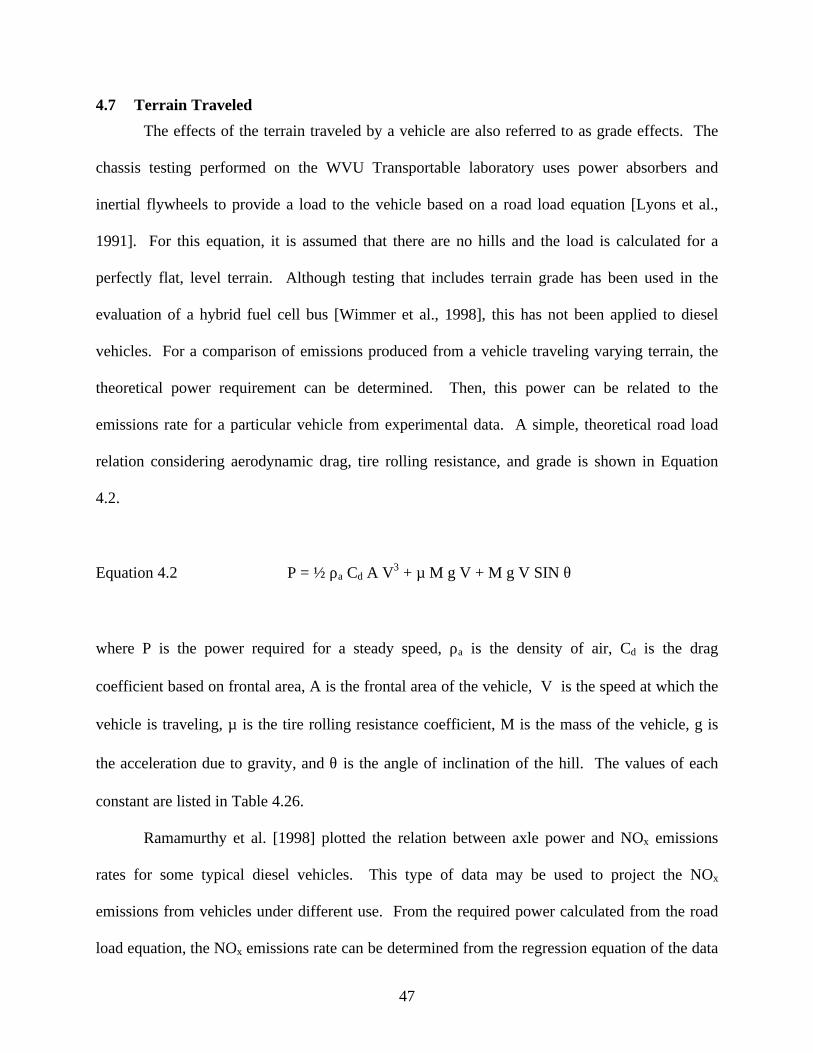
47

4.7 Terrain Traveled

The effects of the terrain traveled by a vehicle are also referred to as grade effects. The

chassis testing performed on the WVU Transportable laboratory uses power absorbers and

inertial flywheels to provide a load to the vehicle based on a road load equation [Lyons et al.,

1991]. For this equation, it is assumed that there are no hills and the load is calculated for a

perfectly flat, level terrain. Although testing that includes terrain grade has been used in the

evaluation of a hybrid fuel cell bus [Wimmer et al., 1998], this has not been applied to diesel

vehicles. For a comparison of emissions produced from a vehicle traveling varying terrain, the

theoretical power requirement can be determined. Then, this power can be related to the

emissions rate for a particular vehicle from experimental data. A simple, theoretical road load

relation considering aerodynamic drag, tire rolling resistance, and grade is shown in Equation

4.2.

Equation 4.2 P = ½ ρa Cd A V3 + µ M g V + M g V SIN θ

where P is the power required for a steady speed, ρa is the density of air, Cd is the drag

coefficient based on frontal area, A is the frontal area of the vehicle, V is the speed at which the

vehicle is traveling, µ is the tire rolling resistance coefficient, M is the mass of the vehicle, g is

the acceleration due to gravity, and θ is the angle of inclination of the hill. The values of each

constant are listed in Table 4.26.

Ramamurthy et al. [1998] plotted the relation between axle power and NOx emissions

rates for some typical diesel vehicles. This type of data may be used to project the NOx

emissions from vehicles under different use. From the required power calculated from the road

load equation, the NOx emissions rate can be determined from the regression equation of the data

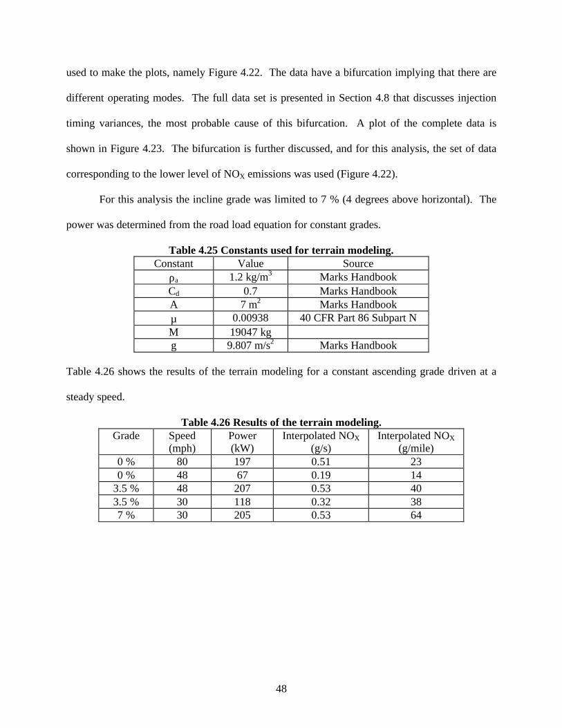
48

used to make the plots, namely Figure 4.22. The data have a bifurcation implying that there are

different operating modes. The full data set is presented in Section 4.8 that discusses injection

timing variances, the most probable cause of this bifurcation. A plot of the complete data is

shown in Figure 4.23. The bifurcation is further discussed, and for this analysis, the set of data

corresponding to the lower level of NOX emissions was used (Figure 4.22).

For this analysis the incline grade was limited to 7 % (4 degrees above horizontal). The

power was determined from the road load equation for constant grades.

Table 4.25 Constants used for terrain modeling.Constant Value Source

ρa 1.2 kg/m3 Marks HandbookCd 0.7 Marks HandbookA 7 m2 Marks Handbookµ 0.00938 40 CFR Part 86 Subpart NM 19047 kgg 9.807 m/s2 Marks Handbook

Table 4.26 shows the results of the terrain modeling for a constant ascending grade driven at a

steady speed.

Table 4.26 Results of the terrain modeling.Grade Speed

(mph)Power(kW)

Interpolated NOX

(g/s)Interpolated NOX

(g/mile)0 % 80 197 0.51 230 % 48 67 0.19 14

3.5 % 48 207 0.53 403.5 % 30 118 0.32 387 % 30 205 0.53 64

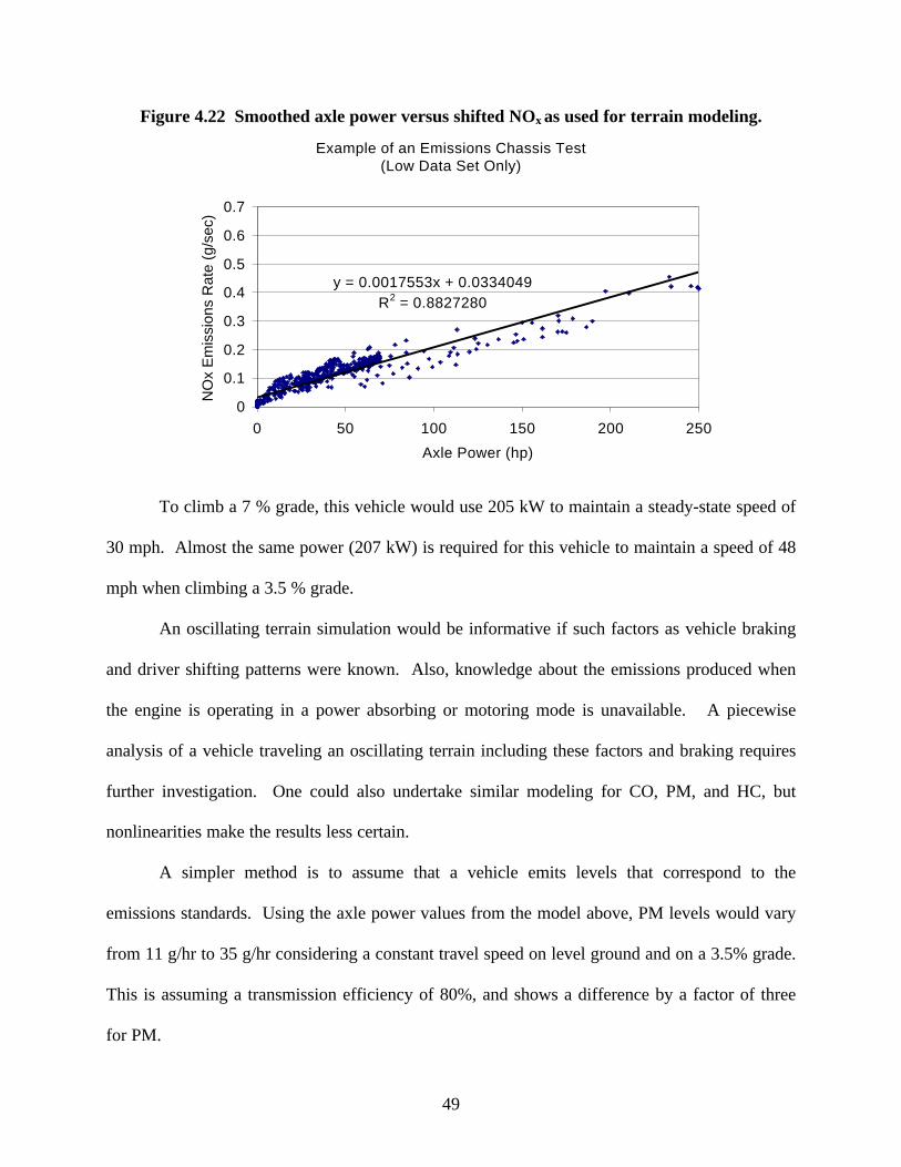
49

Figure 4.22 Smoothed axle power versus shifted NOx as used for terrain modeling.

Example of an Emissions Chassis Test (Low Data Set Only)

y = 0.0017553x + 0.0334049R2 = 0.8827280

0

0.1

0.2

0.3

0.4

0.5

0.6

0.7

0 50 100 150 200 250

Axle Power (hp)

NO

x E

mis

sion

s R

ate

(g/s

ec)

To climb a 7 % grade, this vehicle would use 205 kW to maintain a steady-state speed of

30 mph. Almost the same power (207 kW) is required for this vehicle to maintain a speed of 48

mph when climbing a 3.5 % grade.

An oscillating terrain simulation would be informative if such factors as vehicle braking

and driver shifting patterns were known. Also, knowledge about the emissions produced when

the engine is operating in a power absorbing or motoring mode is unavailable. A piecewise

analysis of a vehicle traveling an oscillating terrain including these factors and braking requires

further investigation. One could also undertake similar modeling for CO, PM, and HC, but

nonlinearities make the results less certain.

A simpler method is to assume that a vehicle emits levels that correspond to the

emissions standards. Using the axle power values from the model above, PM levels would vary

from 11 g/hr to 35 g/hr considering a constant travel speed on level ground and on a 3.5% grade.

This is assuming a transmission efficiency of 80%, and shows a difference by a factor of three

for PM.

50

4.8 Injection Timing Variances

Emissions of NOX and PM are known to be affected strongly by the timing of the in-

cylinder fuel injection in diesel engines. Indeed, it is common to present a hyperbolic “NOX-PM

tradeoff” curve for an engine, with more advanced timing leading to higher NOX, and lower PM.

Within a reasonable operating range, there is also a tradeoff between NOX and efficiency, with

advanced timing leading to a higher NOX and higher thermal efficiency.

Many present day electronically controlled engines do not embody timing throughout

their operating range that reflects the timing employed during the engine certification test.

Deviations in timing during “off-cycle” operation may lead to emissions of NOX that are higher

than those that would occur during the certification test at the same engine speed and load. In

some cases available data suggest a binary timing map, with a “high” and “low” NOX emissions

rate. Since history effects may determine which of the two timing choices is in effect, it is not

always possible to predict unambiguously the NOX emissions rate given the engine torque and

speed.

Figure 4.23 presents a plot of chassis-based NOX emissions versus power output at the

rear axle for a late model diesel truck. These data were obtained by West Virginia University as

part of its field research funded by the U.S. Department of Energy, Office of Transportation

Technologies. The lower NOX data set, when plotted versus axle power, corresponds well to the

line of 6.25 g NOX/ahp-hr (where ahp is horsepower measured at the rear axle). A certification

rate of 5 g/bhp-hr, coupled with an assumed drivetrain efficiency of 80% yields a 6.25 g/ahp-hr

value. The 80% value is offered as an approximation because precise records of transmission

and drivetrain efficiency are not commonly available. The higher NOX data set represents the

“off cycle” operating points.

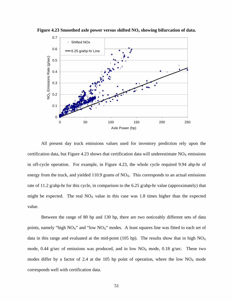
51

Figure 4.23 Smoothed axle power versus shifted NOx showing bifurcation of data.

0

0.1

0.2

0.3

0.4

0.5

0.6

0.7

0 50 100 150 200 250

Axle Power (hp)

NO

X E

mis

sion

s R

ate

(g/s

ec)

Shifted NOx

6.25 g/ahp-hr Line

All present day truck emissions values used for inventory prediction rely upon the

certification data, but Figure 4.23 shows that certification data will underestimate NOX emissions

in off-cycle operation. For example, in Figure 4.23, the whole cycle required 9.94 ahp-hr of

energy from the truck, and yielded 110.9 grams of NOX. This corresponds to an actual emissions

rate of 11.2 g/ahp-hr for this cycle, in comparison to the 6.25 g/ahp-hr value (approximately) that

might be expected. The real NOX value in this case was 1.8 times higher than the expected

value.

Between the range of 80 hp and 130 hp, there are two noticeably different sets of data

points, namely “high NOX” and “low NOX” modes. A least squares line was fitted to each set of

data in this range and evaluated at the mid-point (105 hp). The results show that in high NOX

mode, 0.44 g/sec of emissions was produced, and in low NOX mode, 0.18 g/sec. These two

modes differ by a factor of 2.4 at the 105 hp point of operation, where the low NOX mode

corresponds well with certification data.

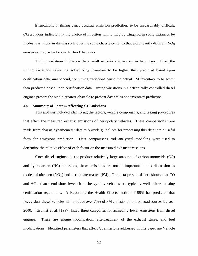
52

Bifurcations in timing cause accurate emission predictions to be unreasonably difficult.

Observations indicate that the choice of injection timing may be triggered in some instances by

modest variations in driving style over the same chassis cycle, so that significantly different NOX

emissions may arise for similar truck behavior.

Timing variations influence the overall emissions inventory in two ways. First, the

timing variations cause the actual NOX inventory to be higher than predicted based upon

certification data, and second, the timing variations cause the actual PM inventory to be lower

than predicted based upon certification data. Timing variations in electronically controlled diesel

engines present the single greatest obstacle to present day emissions inventory prediction.

4.9 Summary of Factors Affecting CI Emissions

This analysis included identifying the factors, vehicle components, and testing procedures

that effect the measured exhaust emissions of heavy-duty vehicles. These comparisons were

made from chassis dynamometer data to provide guidelines for processing this data into a useful

form for emissions prediction. Data comparisons and analytical modeling were used to

determine the relative effect of each factor on the measured exhaust emissions.

Since diesel engines do not produce relatively large amounts of carbon monoxide (CO)

and hydrocarbon (HC) emissions, these emissions are not as important in this discussion as

oxides of nitrogen (NOX) and particulate matter (PM). The data presented here shows that CO

and HC exhaust emissions levels from heavy-duty vehicles are typically well below existing

certification regulations. A Report by the Health Effects Institute [1995] has predicted that

heavy-duty diesel vehicles will produce over 75% of PM emissions from on-road sources by year

2000. Grumet et al. [1997] listed three categories for achieving lower emissions from diesel

engines. These are engine modification, aftertreatment of the exhaust gases, and fuel

modifications. Identified parameters that affect CI emissions addressed in this paper are Vehicle

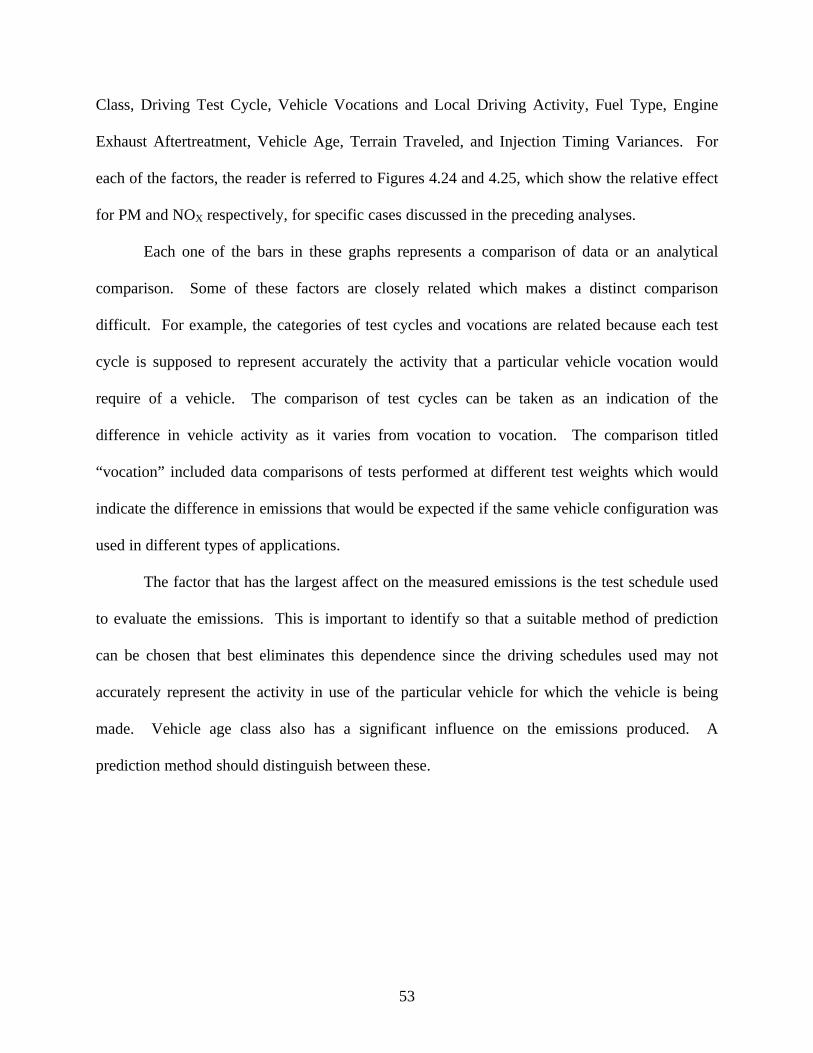
53

Class, Driving Test Cycle, Vehicle Vocations and Local Driving Activity, Fuel Type, Engine

Exhaust Aftertreatment, Vehicle Age, Terrain Traveled, and Injection Timing Variances. For

each of the factors, the reader is referred to Figures 4.24 and 4.25, which show the relative effect

for PM and NOX respectively, for specific cases discussed in the preceding analyses.

Each one of the bars in these graphs represents a comparison of data or an analytical

comparison. Some of these factors are closely related which makes a distinct comparison

difficult. For example, the categories of test cycles and vocations are related because each test

cycle is supposed to represent accurately the activity that a particular vehicle vocation would

require of a vehicle. The comparison of test cycles can be taken as an indication of the

difference in vehicle activity as it varies from vocation to vocation. The comparison titled

“vocation” included data comparisons of tests performed at different test weights which would

indicate the difference in emissions that would be expected if the same vehicle configuration was

used in different types of applications.

The factor that has the largest affect on the measured emissions is the test schedule used

to evaluate the emissions. This is important to identify so that a suitable method of prediction

can be chosen that best eliminates this dependence since the driving schedules used may not

accurately represent the activity in use of the particular vehicle for which the vehicle is being

made. Vehicle age class also has a significant influence on the emissions produced. A

prediction method should distinguish between these.

54

Figure 4.24 Effect of various factors on particulate matter emissions. Each bar representsa specific comparison discussed in the text and cannot be taken to represent all cases

encountered.

30%

1500%

200%60%

350%

1200%

300%

0%

200%

400%

600%

800%

1000%

1200%

1400%

1600%

1800%

Class

Cycles

Vocatio

nsFuel

Aftertr

eatm

ent

Age

Terra

in

Injec

tion T

imin

g

Eff

ect

on

Em

issi

on

s

Un

kno

wn

Figure 4.25 Effect of various factors on oxides of nitrogen emissions. Each bar represents aspecific comparison discussed in the text and cannot be taken to represent all cases

encountered.

25%

300%

10%25% 15%

250% 250%

200%

0%

50%

100%

150%

200%

250%

300%

350%

Class

Cycles

Vocat

ions

Fuel

Aftertr

eatm

ent

Age

Terra

in

Injec

tion

Timing

Effe

ct o

n E

mis

sion

s

55

5. Methods of Generating Emissions Factors

These methods presented here are similar to research options currently being evaluated

by West Virginia University for prediction of heavy-duty truck emissions for NCHRP. Various

approaches exist or can be suggested for the prediction of heavy vehicle emissions contribution

to the national or a regional inventory. In the absence of accurate measurement of emissions

from every vehicle performing every task, all approaches must be an approximation and it may

prove impossible with current data to hold any approach superior to another. Prediction of

emissions is confounded by a lack of detailed data on vehicle activity, a database of heavy-duty

vehicle emissions measurements far smaller than that for automobiles, and the unquantified

effects of operating parameters on the diesel exhaust produced by vehicles.

5.1 Certification Data

The present approach to prediction of emissions output from heavy-duty vehicles relies

on the use of emissions certification data to yield, for each species, an emissions factor with units

of g/bhp-hr. The Federal Testing Procedure (FTP) is a transient stationary dynamometer test

used to evaluate an engine’s emission production level for federal certification. The target

values (engine speed and load values) were arrived at through the use of a Monte Carlo

simulation of data collected in Los Angeles, CA and New York, NY in the early 1970’s. The

vehicles represented in the study had a lower power-to-weight ratio than current highly

turbocharged diesel powered heavy-duty vehicles, and some vehicles in this study were gasoline

powered.

Emissions factors for heavy-duty vehicles are usually expressed in grams per mile

(g/mile). The emissions certification data for the engines that power these vehicles are in units

of grams per brake horsepower-hour (g/bhp-hr). One method of converting the certification data

56

to vehicle emissions is to use the formula from Machiele (1988). To use this method, the

conversion factor of brake horsepower-hour per mile (bhp-hr/mile) of the vehicle needs to be

found. This is done using the fuel density, fuel energy content and fuel economy of the vehicle.

The formula for vehicle emissions in g/mile is shown in Equation 5.1.

Equation 5.1

−

−

=mile

gallons

lbs

hrbhp

gallon

lbs

hrbhp

g

mile

g

Figure 5.1 shows the trend of emissions of a vehicle that achieves a fuel economy of 3.0

miles per gallon and has a brake specific fuel consumption of 0.5 pounds per brake horsepower-

hour. These values are from the representative data given in Machiele’s report for a 1980’s

vintage diesel vehicle. The emissions factors in g/mile are then multiplied by vehicle miles

traveled (VMT) to yield the mass of emissions released into the environment. The emissions

factors can also be expressed in terms of grams per second (g/sec) if the speed of the vehicle is

known.

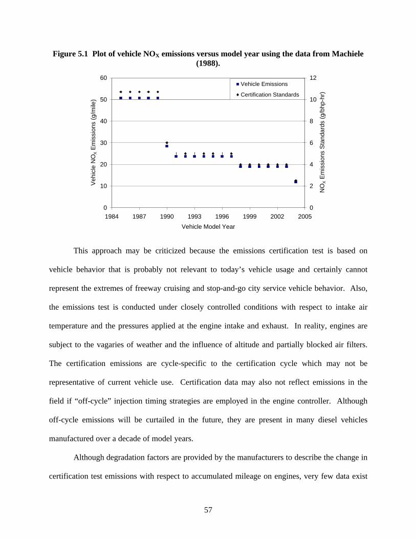
57

Figure 5.1 Plot of vehicle NOX emissions versus model year using the data from Machiele(1988).

0

10

20

30

40

50

60

1984 1987 1990 1993 1996 1999 2002 2005

Vehicle Model Year

Veh

icle

NO

X E

mis

sion

s (g

/mile

)

0

2

4

6

8

10

12

NO

X E

mis

sion

s S

tand

ards

(g/

bhp-

hr)

Vehicle Emissions

Certification Standards

This approach may be criticized because the emissions certification test is based on

vehicle behavior that is probably not relevant to today’s vehicle usage and certainly cannot

represent the extremes of freeway cruising and stop-and-go city service vehicle behavior. Also,

the emissions test is conducted under closely controlled conditions with respect to intake air

temperature and the pressures applied at the engine intake and exhaust. In reality, engines are

subject to the vagaries of weather and the influence of altitude and partially blocked air filters.

The certification emissions are cycle-specific to the certification cycle which may not be

representative of current vehicle use. Certification data may also not reflect emissions in the

field if “off-cycle” injection timing strategies are employed in the engine controller. Although

off-cycle emissions will be curtailed in the future, they are present in many diesel vehicles

manufactured over a decade of model years.

Although degradation factors are provided by the manufacturers to describe the change in

certification test emissions with respect to accumulated mileage on engines, very few data exist

58

to show emissions decline in real use. These factors do not account for engines that have endured

tampering or malfunction or are approaching retirement or rebuild age. Some effects of

tampering have been described by McKain et al. (1998), although the authors expect tampering

on transit buses not to be a substantial influence. The emissions factors therefore do not reflect

the spectrum of vehicle maintenance conditions in use, although it is the opinion of the authors

that diesel engine emissions remain more stable than those from spark-ignited engines as the

vehicles age. Concerns over effect of vehicle condition will rise as exhaust aftertreatment

devices become prevalent in use.

Further inaccuracies arise in this approach due to the uncertainty in fuel energy content

and vehicle fuel consumption. It is evident that fuel consumption is highly dependent on vehicle

vocation and on the combination of engine, transmission and vehicle configuration.

5.2 Chassis Dynamometer Data

Heavy-duty vehicles may be subjected to emissions characterization on a chassis

dynamometer, as is the present approach for light duty vehicles (Clark et al., 1995; Graboski et

al., 1998; Deitzman et al., 1985). The emissions results may be obtained directly in g/mile for

each emissions constituent. A simple approach for prediction therefore involves taking the

product of these emissions factors and the vehicle miles traveled. This approach is at least as

valid as the present approach and offers the advantage that fuel economy need not be considered

in the process. All else being equal, a vehicle with a less efficient drivetrain would simply yield

higher emissions factors in units of grams per mile (g/mile).

There is the advantage that vehicles subjected to chassis dynamometer emissions

characterization can be tested as received, including influences of tampering or malfunction that

might be lost if the engine were first removed from the vehicle. There is also the advantage that

vehicles are more readily tested using chassis dynamometer systems than by removing the

59

engine from the vehicle, so that data more representative of the whole fleet, rather than new

vehicles, can be obtained.

A problem arises in that no single cycle can hope to represent the real world spectrum of

vehicle activities. Although the Urban Dynamometer Driving Schedule (Test-D) (40 CFR, Part

86) exists as a companion to the engine certification test, it does not correlate well with the

engine certification test (Deitzman and Warner-Selph, 1985) and does not represent all

behaviors. Although future information may be gathered to yield a few representative emissions

test cycles for the fleet, these will be applicable only to future testing and existing chassis cycle

data will not be useful.

It is certain that the test cycle used has profound effect to the emissions yielded. Based on

these data, the approach of using direct chassis dynamometer data for emissions inventory has

appeal only for future testing following the development of a suite of cycles that are acceptably

representative of fleet behavior, considering regional and vocational differences.

A portion of testing at WVU involved testing a single truck on 19 different test cycles.

The results of NOX in g/mile are shown in Figure 5.2. These data are preliminary and details of

the testing will be published at a later date. The vehicle was a 1995 GMC box truck with a

Caterpillar 3116 engine rated at 170hp. The fuel used was D2 diesel and the vehicle has a

GVWR of 22,000 pounds. The engine in this vehicle employed a mechanical fuel-injection

system so no off-cycle emissions schemes were possible. There is further data on the influence

of cycles on emissions from a city bus in Clark et al. (1997). Figure 5.3 shows the emissions

data for the 1996 New Flyer transit bus which was powered by a Detroit Diesel Series 50 engine.

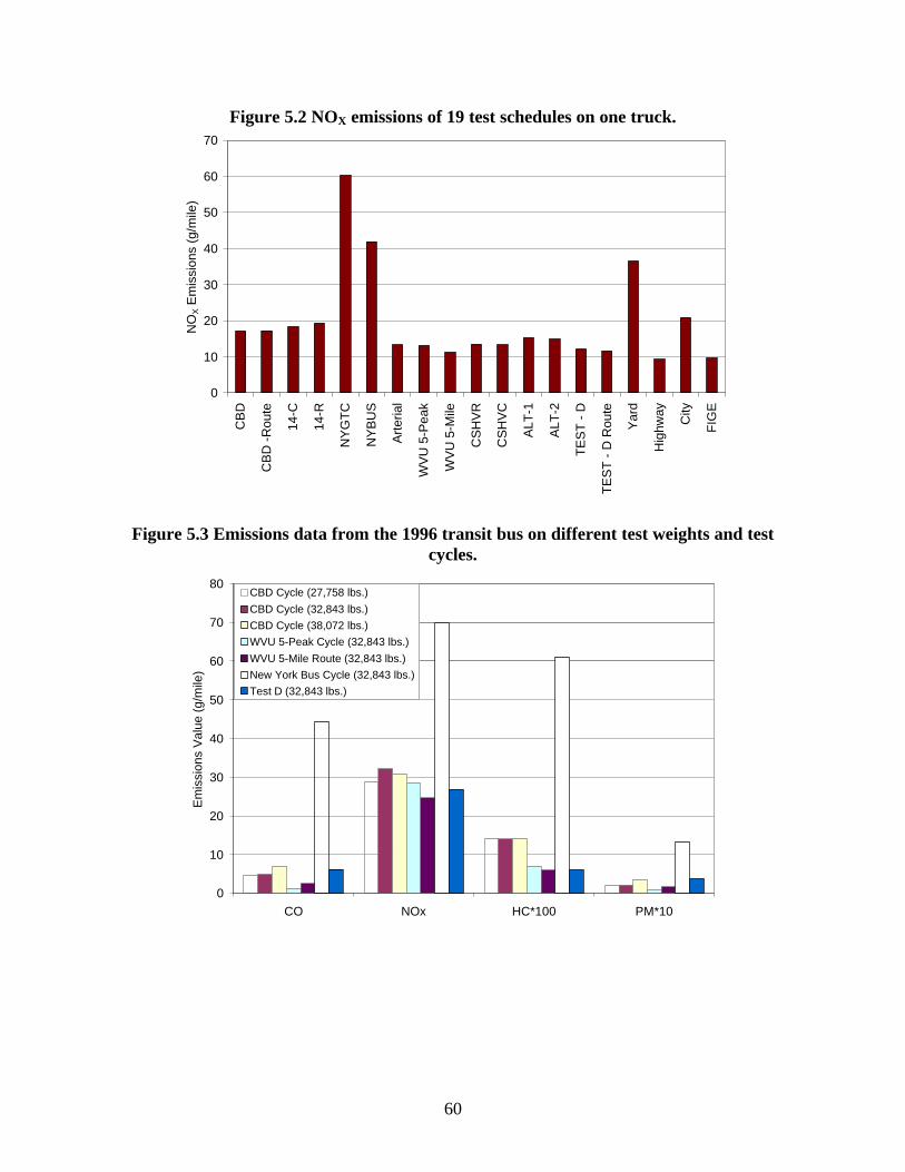
60

Figure 5.2 NOX emissions of 19 test schedules on one truck.

0

10

20

30

40

50

60

70

CB

D

CB

D -

Rou

te

14-C

14-R

NY

GT

C

NY

BU

S

Art

eria

l

WV

U 5

-Pea

k

WV

U 5

-Mile

CS

HV

R

CS

HV

C

ALT

-1

ALT

-2

TE

ST

- D

TE

ST

- D

Rou

te

Yar

d

Hig

hway

City

FIG

E

NO

X E

mis

sion

s (g

/mile

)

Figure 5.3 Emissions data from the 1996 transit bus on different test weights and testcycles.

0

10

20

30

40

50

60

70

80

CO NOx HC*100 PM*10

Em

issi

ons

Val

ue (

g/m

ile)

CBD Cycle (27,758 lbs.)



WVU 5-Peak Cycle (32,843 lbs.)

WVU 5-Mile Route (32,843 lbs.)

New York Bus Cycle (32,843 lbs.)

Test D (32,843 lbs.)

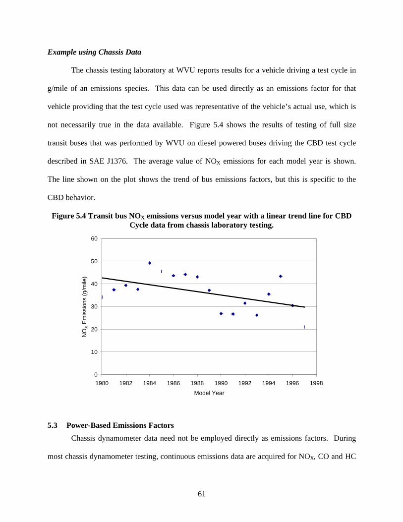
61

Example using Chassis Data

The chassis testing laboratory at WVU reports results for a vehicle driving a test cycle in

g/mile of an emissions species. This data can be used directly as an emissions factor for that

vehicle providing that the test cycle used was representative of the vehicle’s actual use, which is

not necessarily true in the data available. Figure 5.4 shows the results of testing of full size

transit buses that was performed by WVU on diesel powered buses driving the CBD test cycle

described in SAE J1376. The average value of NOX emissions for each model year is shown.

The line shown on the plot shows the trend of bus emissions factors, but this is specific to the

CBD behavior.

Figure 5.4 Transit bus NOX emissions versus model year with a linear trend line for CBDCycle data from chassis laboratory testing.

0

10

20

30

40

50

60

1980 1982 1984 1986 1988 1990 1992 1994 1996 1998

Model Year

NO

X E

mis

sion

s (g

/mile

)

5.3 Power-Based Emissions Factors

Chassis dynamometer data need not be employed directly as emissions factors. During

most chassis dynamometer testing, continuous emissions data are acquired for NOX, CO and HC

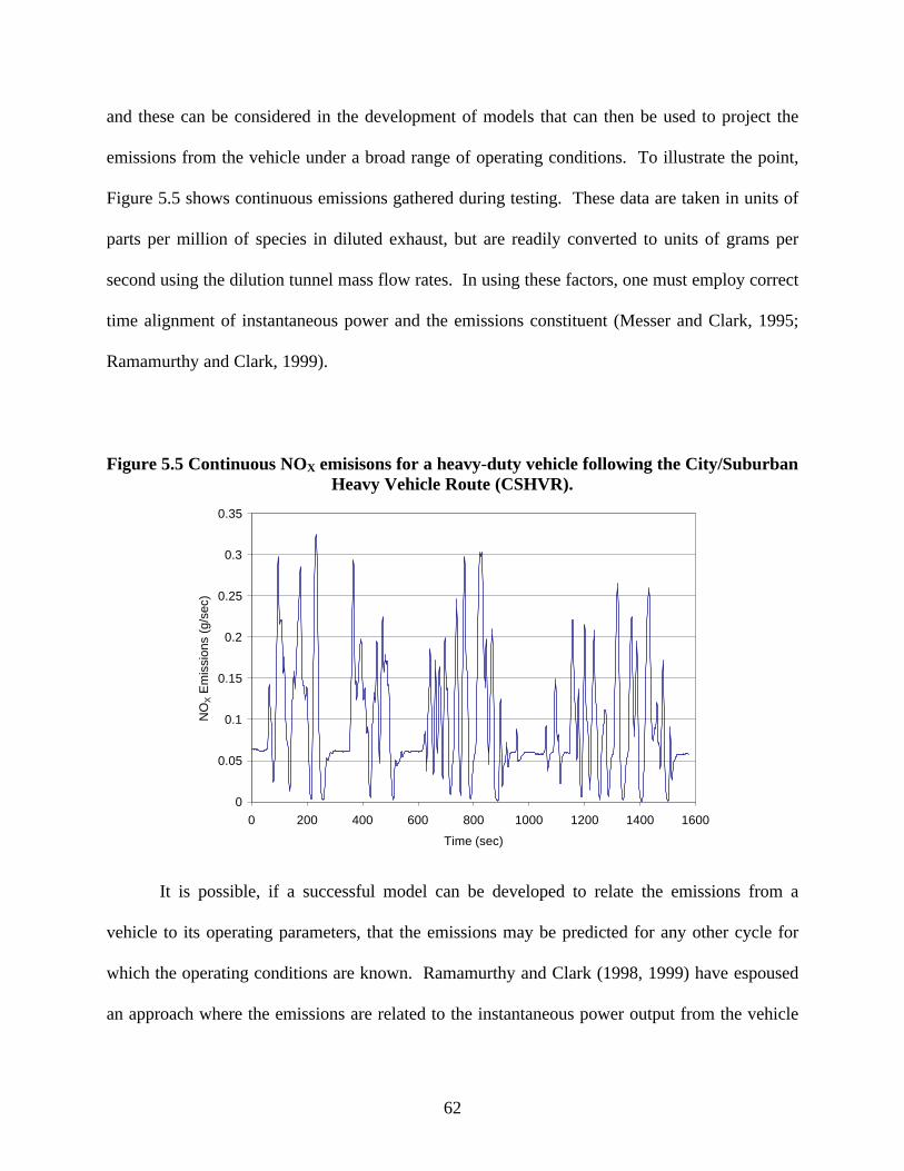
62

and these can be considered in the development of models that can then be used to project the

emissions from the vehicle under a broad range of operating conditions. To illustrate the point,

Figure 5.5 shows continuous emissions gathered during testing. These data are taken in units of

parts per million of species in diluted exhaust, but are readily converted to units of grams per

second using the dilution tunnel mass flow rates. In using these factors, one must employ correct

time alignment of instantaneous power and the emissions constituent (Messer and Clark, 1995;

Ramamurthy and Clark, 1999).

Figure 5.5 Continuous NOX emisisons for a heavy-duty vehicle following the City/SuburbanHeavy Vehicle Route (CSHVR).

0

0.05

0.1

0.15

0.2

0.25

0.3

0.35

0 200 400 600 800 1000 1200 1400 1600

Time (sec)

NO

X E

mis

sion

s (g

/sec

)

It is possible, if a successful model can be developed to relate the emissions from a

vehicle to its operating parameters, that the emissions may be predicted for any other cycle for

which the operating conditions are known. Ramamurthy and Clark (1998, 1999) have espoused

an approach where the emissions are related to the instantaneous power output from the vehicle

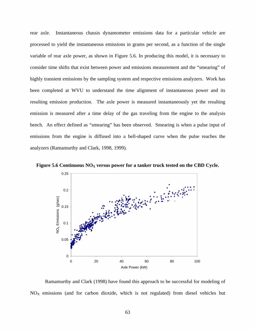
63

rear axle. Instantaneous chassis dynamometer emissions data for a particular vehicle are

processed to yield the instantaneous emissions in grams per second, as a function of the single

variable of rear axle power, as shown in Figure 5.6. In producing this model, it is necessary to

consider time shifts that exist between power and emissions measurement and the “smearing” of

highly transient emissions by the sampling system and respective emissions analyzers. Work has

been completed at WVU to understand the time alignment of instantaneous power and its

resulting emission production. The axle power is measured instantaneously yet the resulting

emission is measured after a time delay of the gas traveling from the engine to the analysis

bench. An effect defined as “smearing” has been observed. Smearing is when a pulse input of

emissions from the engine is diffused into a bell-shaped curve when the pulse reaches the

analyzers (Ramamurthy and Clark, 1998, 1999).

Figure 5.6 Continuous NOX versus power for a tanker truck tested on the CBD Cycle.

0

0.05

0.1

0.15

0.2

0.25

0 20 40 60 80 100

Axle Power (kW)

NO

X E

mis

sion

s (

g/se

c)

Ramamurthy and Clark (1998) have found this approach to be successful for modeling of

NOX emissions (and for carbon dioxide, which is not regulated) from diesel vehicles but

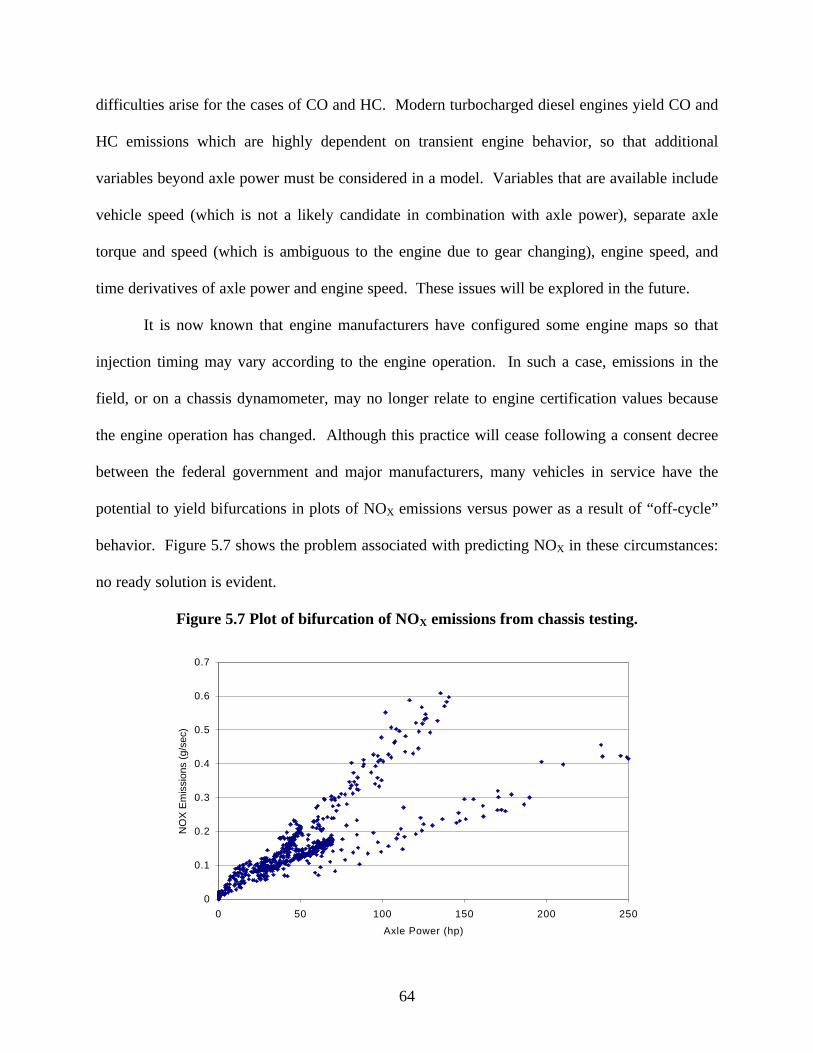
64

difficulties arise for the cases of CO and HC. Modern turbocharged diesel engines yield CO and

HC emissions which are highly dependent on transient engine behavior, so that additional

variables beyond axle power must be considered in a model. Variables that are available include

vehicle speed (which is not a likely candidate in combination with axle power), separate axle

torque and speed (which is ambiguous to the engine due to gear changing), engine speed, and

time derivatives of axle power and engine speed. These issues will be explored in the future.

It is now known that engine manufacturers have configured some engine maps so that

injection timing may vary according to the engine operation. In such a case, emissions in the

field, or on a chassis dynamometer, may no longer relate to engine certification values because

the engine operation has changed. Although this practice will cease following a consent decree

between the federal government and major manufacturers, many vehicles in service have the

potential to yield bifurcations in plots of NOX emissions versus power as a result of “off-cycle”

behavior. Figure 5.7 shows the problem associated with predicting NOX in these circumstances:

no ready solution is evident.

Figure 5.7 Plot of bifurcation of NOX emissions from chassis testing.

0

0.1

0.2

0.3

0.4

0.5

0.6

0.7

0 50 100 150 200 250

Axle Power (hp)

NO

X E

mis

sion

s (g

/sec

)

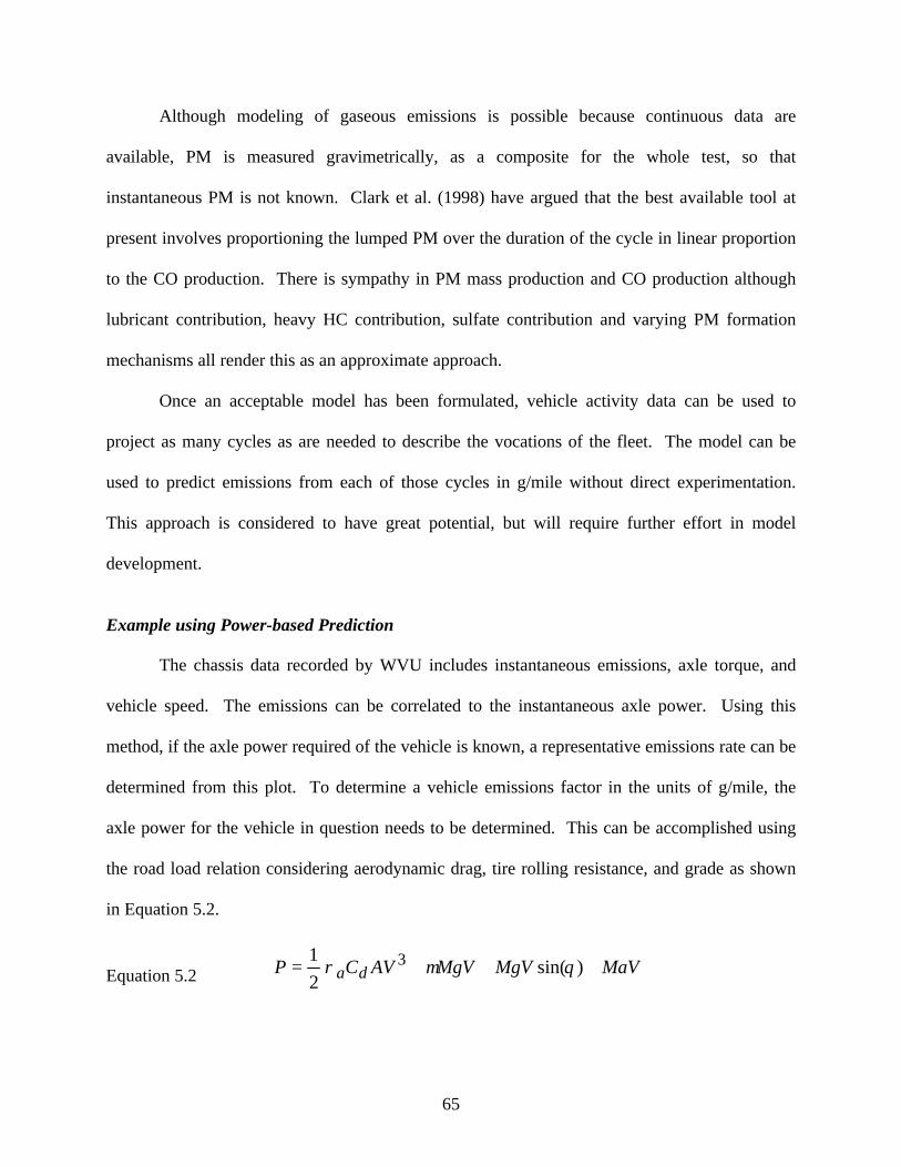
65

Although modeling of gaseous emissions is possible because continuous data are

available, PM is measured gravimetrically, as a composite for the whole test, so that

instantaneous PM is not known. Clark et al. (1998) have argued that the best available tool at

present involves proportioning the lumped PM over the duration of the cycle in linear proportion

to the CO production. There is sympathy in PM mass production and CO production although

lubricant contribution, heavy HC contribution, sulfate contribution and varying PM formation

mechanisms all render this as an approximate approach.

Once an acceptable model has been formulated, vehicle activity data can be used to

project as many cycles as are needed to describe the vocations of the fleet. The model can be

used to predict emissions from each of those cycles in g/mile without direct experimentation.

This approach is considered to have great potential, but will require further effort in model

development.

Example using Power-based Prediction

The chassis data recorded by WVU includes instantaneous emissions, axle torque, and

vehicle speed. The emissions can be correlated to the instantaneous axle power. Using this

method, if the axle power required of the vehicle is known, a representative emissions rate can be

determined from this plot. To determine a vehicle emissions factor in the units of g/mile, the

axle power for the vehicle in question needs to be determined. This can be accomplished using

the road load relation considering aerodynamic drag, tire rolling resistance, and grade as shown

in Equation 5.2.

Equation 5.2 MaVMgVMgVAVCP da +++= )sin(2

1 3 θµρ

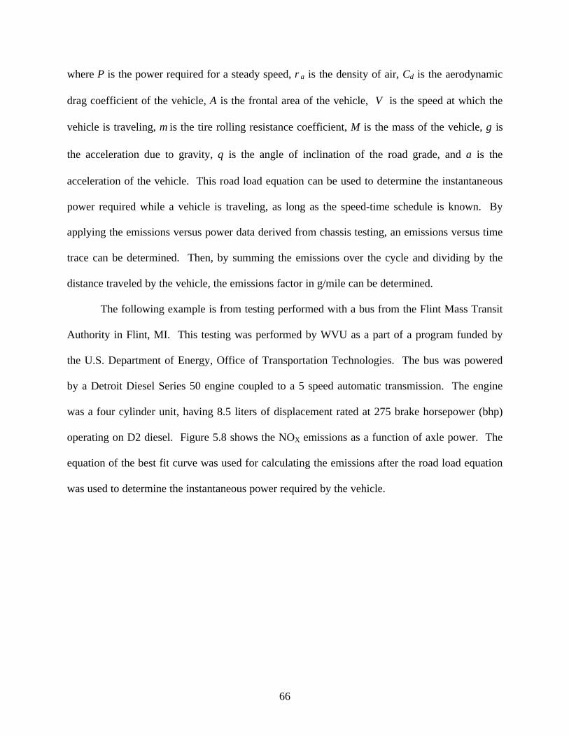
66

where P is the power required for a steady speed, ρa is the density of air, Cd is the aerodynamic

drag coefficient of the vehicle, A is the frontal area of the vehicle, V is the speed at which the

vehicle is traveling, µ is the tire rolling resistance coefficient, M is the mass of the vehicle, g is

the acceleration due to gravity, θ is the angle of inclination of the road grade, and a is the

acceleration of the vehicle. This road load equation can be used to determine the instantaneous

power required while a vehicle is traveling, as long as the speed-time schedule is known. By

applying the emissions versus power data derived from chassis testing, an emissions versus time

trace can be determined. Then, by summing the emissions over the cycle and dividing by the

distance traveled by the vehicle, the emissions factor in g/mile can be determined.

The following example is from testing performed with a bus from the Flint Mass Transit

Authority in Flint, MI. This testing was performed by WVU as a part of a program funded by

the U.S. Department of Energy, Office of Transportation Technologies. The bus was powered

by a Detroit Diesel Series 50 engine coupled to a 5 speed automatic transmission. The engine

was a four cylinder unit, having 8.5 liters of displacement rated at 275 brake horsepower (bhp)

operating on D2 diesel. Figure 5.8 shows the NOX emissions as a function of axle power. The

equation of the best fit curve was used for calculating the emissions after the road load equation

was used to determine the instantaneous power required by the vehicle.

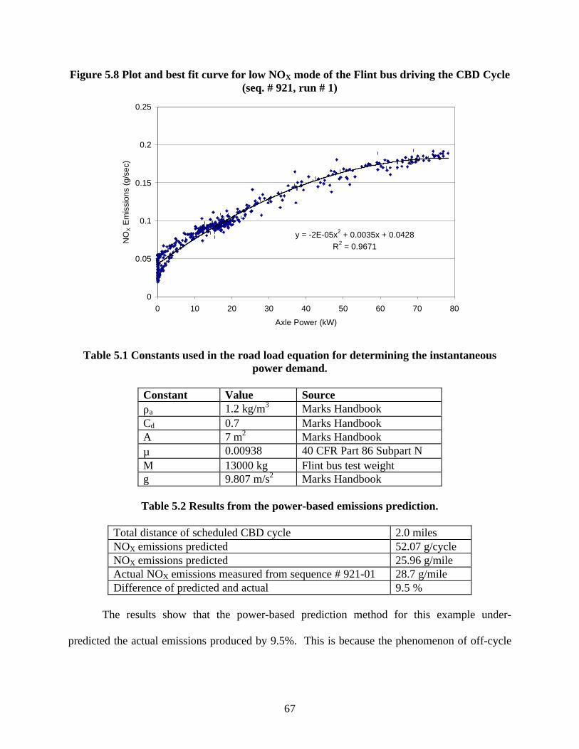
67

Figure 5.8 Plot and best fit curve for low NOX mode of the Flint bus driving the CBD Cycle(seq. # 921, run # 1)

y = -2E-05x2 + 0.0035x + 0.0428R2 = 0.9671

0

0.05

0.1

0.15

0.2

0.25

0 10 20 30 40 50 60 70 80

Axle Power (kW)

NO

X E

mis

sion

s (g

/sec

)

Table 5.1 Constants used in the road load equation for determining the instantaneouspower demand.

Constant Value Sourceρa 1.2 kg/m3 Marks HandbookCd 0.7 Marks HandbookA 7 m2 Marks Handbookµ 0.00938 40 CFR Part 86 Subpart NM 13000 kg Flint bus test weightg 9.807 m/s2 Marks Handbook

Table 5.2 Results from the power-based emissions prediction.

Total distance of scheduled CBD cycle 2.0 milesNOX emissions predicted 52.07 g/cycleNOX emissions predicted 25.96 g/mileActual NOX emissions measured from sequence # 921-01 28.7 g/mileDifference of predicted and actual 9.5 %

The results show that the power-based prediction method for this example under-

predicted the actual emissions produced by 9.5%. This is because the phenomenon of off-cycle

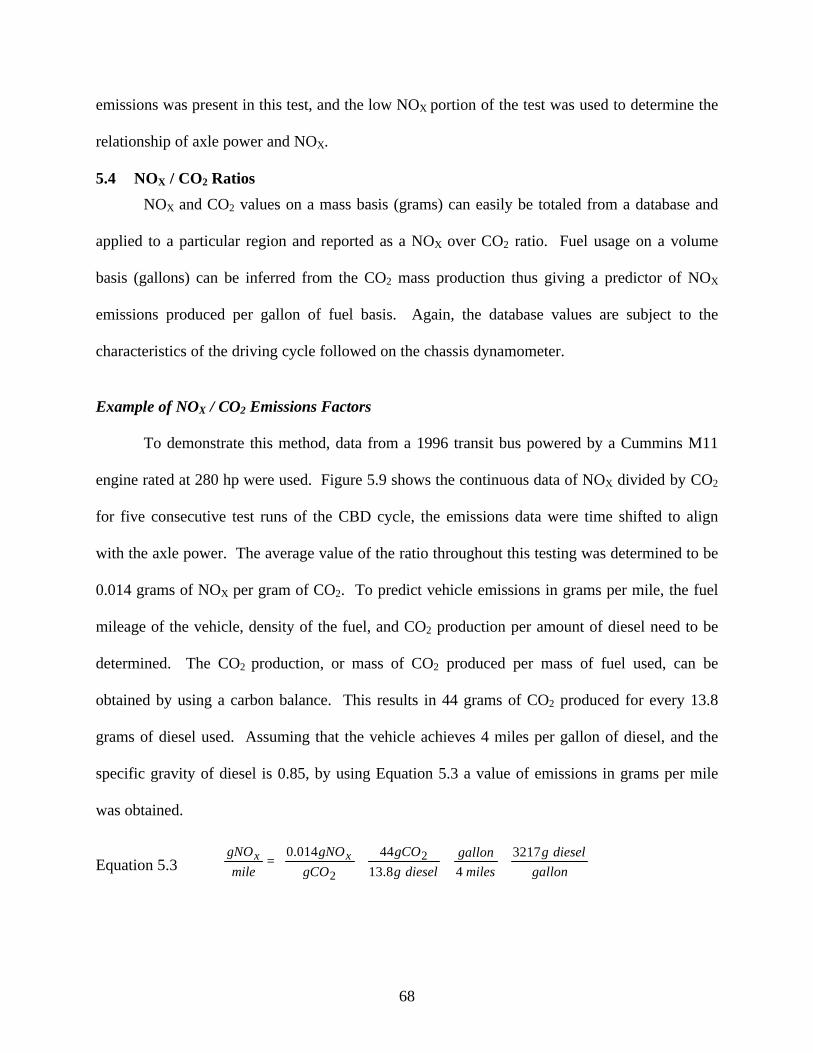
68

emissions was present in this test, and the low NOX portion of the test was used to determine the

relationship of axle power and NOX.

5.4 NOX / CO2 Ratios

NOX and CO2 values on a mass basis (grams) can easily be totaled from a database and

applied to a particular region and reported as a NOX over CO2 ratio. Fuel usage on a volume

basis (gallons) can be inferred from the CO2 mass production thus giving a predictor of NOX

emissions produced per gallon of fuel basis. Again, the database values are subject to the

characteristics of the driving cycle followed on the chassis dynamometer.

Example of NOX / CO2 Emissions Factors

To demonstrate this method, data from a 1996 transit bus powered by a Cummins M11

engine rated at 280 hp were used. Figure 5.9 shows the continuous data of NOX divided by CO2

for five consecutive test runs of the CBD cycle, the emissions data were time shifted to align

with the axle power. The average value of the ratio throughout this testing was determined to be

0.014 grams of NOX per gram of CO2. To predict vehicle emissions in grams per mile, the fuel

mileage of the vehicle, density of the fuel, and CO2 production per amount of diesel need to be

determined. The CO2 production, or mass of CO2 produced per mass of fuel used, can be

obtained by using a carbon balance. This results in 44 grams of CO2 produced for every 13.8

grams of diesel used. Assuming that the vehicle achieves 4 miles per gallon of diesel, and the

specific gravity of diesel is 0.85, by using Equation 5.3 a value of emissions in grams per mile

was obtained.

Equation 5.3

=

gallon

dieselg

miles

gallon

dieselg

gCO

gCO

gNO

mile

gNO xx 3217

48.13

44014.0 2

2

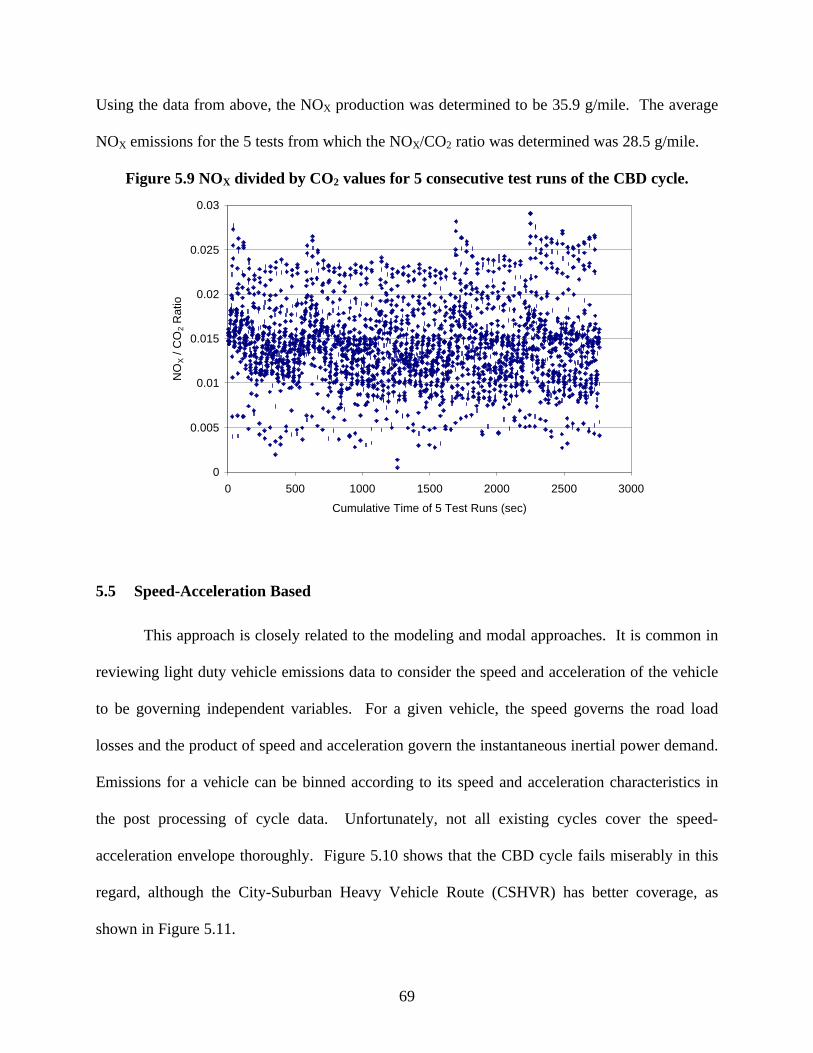
69

Using the data from above, the NOX production was determined to be 35.9 g/mile. The average

NOX emissions for the 5 tests from which the NOX/CO2 ratio was determined was 28.5 g/mile.

Figure 5.9 NOX divided by CO2 values for 5 consecutive test runs of the CBD cycle.

0

0.005

0.01

0.015

0.02

0.025

0.03

0 500 1000 1500 2000 2500 3000

Cumulative Time of 5 Test Runs (sec)

NO

X /

CO

2 R

atio

5.5 Speed-Acceleration Based

This approach is closely related to the modeling and modal approaches. It is common in

reviewing light duty vehicle emissions data to consider the speed and acceleration of the vehicle

to be governing independent variables. For a given vehicle, the speed governs the road load

losses and the product of speed and acceleration govern the instantaneous inertial power demand.

Emissions for a vehicle can be binned according to its speed and acceleration characteristics in

the post processing of cycle data. Unfortunately, not all existing cycles cover the speed-

acceleration envelope thoroughly. Figure 5.10 shows that the CBD cycle fails miserably in this

regard, although the City-Suburban Heavy Vehicle Route (CSHVR) has better coverage, as

shown in Figure 5.11.

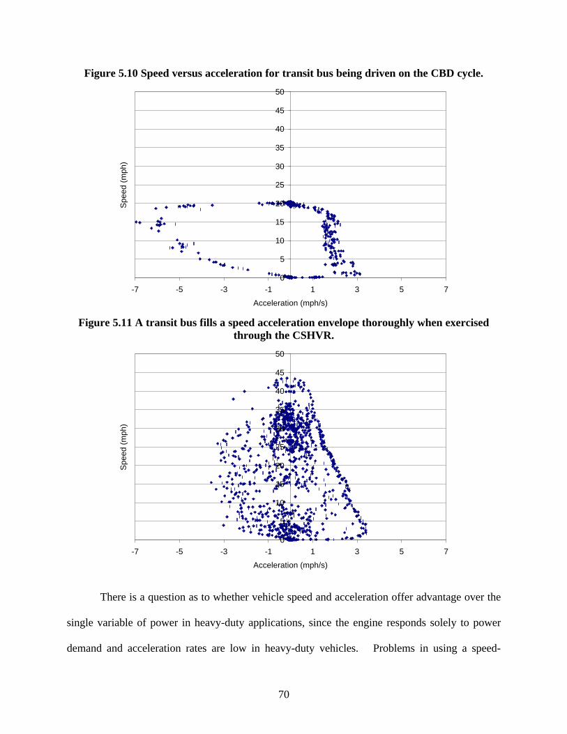
70

Figure 5.10 Speed versus acceleration for transit bus being driven on the CBD cycle.

0

5

10

15

20

25

30

35

40

45

50

-7 -5 -3 -1 1 3 5 7

Acceleration (mph/s)

Spe

ed (

mph

)

Figure 5.11 A transit bus fills a speed acceleration envelope thoroughly when exercisedthrough the CSHVR.

0

5

10

15

20

25

30

35

40

45

50

-7 -5 -3 -1 1 3 5 7


Spe

ed (

mph

)

There is a question as to whether vehicle speed and acceleration offer advantage over the

single variable of power in heavy-duty applications, since the engine responds solely to power

demand and acceleration rates are low in heavy-duty vehicles. Problems in using a speed-

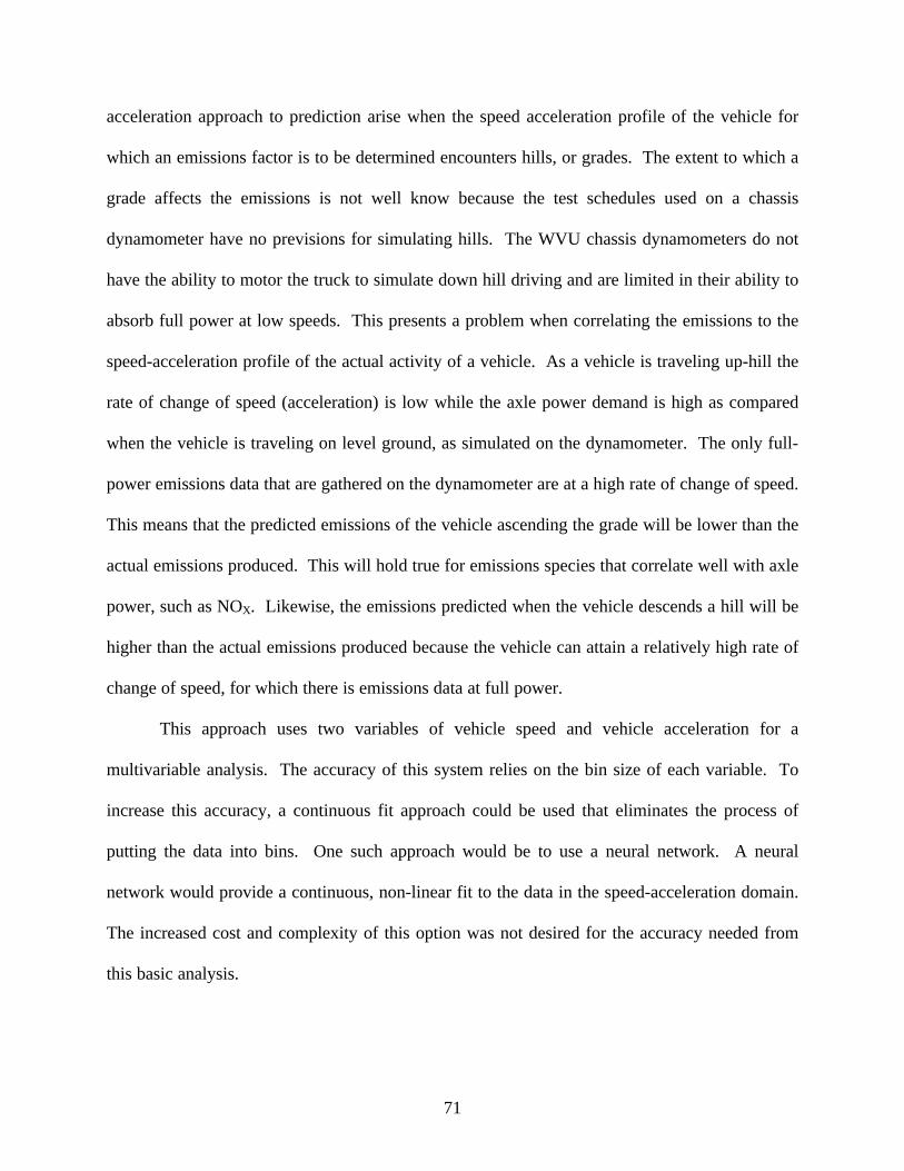
71

acceleration approach to prediction arise when the speed acceleration profile of the vehicle for

which an emissions factor is to be determined encounters hills, or grades. The extent to which a

grade affects the emissions is not well know because the test schedules used on a chassis

dynamometer have no previsions for simulating hills. The WVU chassis dynamometers do not

have the ability to motor the truck to simulate down hill driving and are limited in their ability to

absorb full power at low speeds. This presents a problem when correlating the emissions to the

speed-acceleration profile of the actual activity of a vehicle. As a vehicle is traveling up-hill the

rate of change of speed (acceleration) is low while the axle power demand is high as compared

when the vehicle is traveling on level ground, as simulated on the dynamometer. The only full-

power emissions data that are gathered on the dynamometer are at a high rate of change of speed.

This means that the predicted emissions of the vehicle ascending the grade will be lower than the

actual emissions produced. This will hold true for emissions species that correlate well with axle

power, such as NOX. Likewise, the emissions predicted when the vehicle descends a hill will be

higher than the actual emissions produced because the vehicle can attain a relatively high rate of

change of speed, for which there is emissions data at full power.

This approach uses two variables of vehicle speed and vehicle acceleration for a

multivariable analysis. The accuracy of this system relies on the bin size of each variable. To

increase this accuracy, a continuous fit approach could be used that eliminates the process of

putting the data into bins. One such approach would be to use a neural network. A neural

network would provide a continuous, non-linear fit to the data in the speed-acceleration domain.

The increased cost and complexity of this option was not desired for the accuracy needed from

this basic analysis.

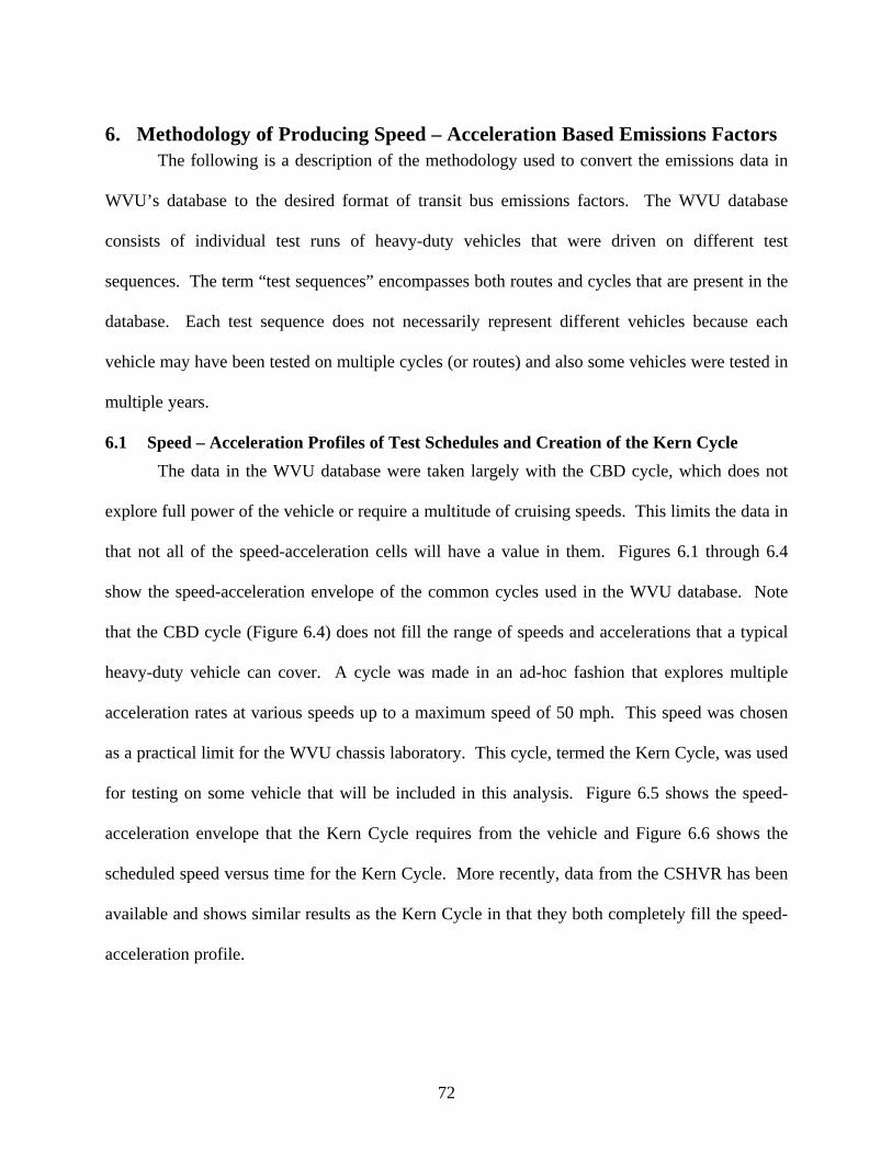
72

6. Methodology of Producing Speed – Acceleration Based Emissions FactorsThe following is a description of the methodology used to convert the emissions data in

WVU’s database to the desired format of transit bus emissions factors. The WVU database

consists of individual test runs of heavy-duty vehicles that were driven on different test

sequences. The term “test sequences” encompasses both routes and cycles that are present in the

database. Each test sequence does not necessarily represent different vehicles because each

vehicle may have been tested on multiple cycles (or routes) and also some vehicles were tested in

multiple years.

6.1 Speed – Acceleration Profiles of Test Schedules and Creation of the Kern Cycle

The data in the WVU database were taken largely with the CBD cycle, which does not

explore full power of the vehicle or require a multitude of cruising speeds. This limits the data in

that not all of the speed-acceleration cells will have a value in them. Figures 6.1 through 6.4

show the speed-acceleration envelope of the common cycles used in the WVU database. Note

that the CBD cycle (Figure 6.4) does not fill the range of speeds and accelerations that a typical

heavy-duty vehicle can cover. A cycle was made in an ad-hoc fashion that explores multiple

acceleration rates at various speeds up to a maximum speed of 50 mph. This speed was chosen

as a practical limit for the WVU chassis laboratory. This cycle, termed the Kern Cycle, was used

for testing on some vehicle that will be included in this analysis. Figure 6.5 shows the speed-

acceleration envelope that the Kern Cycle requires from the vehicle and Figure 6.6 shows the

scheduled speed versus time for the Kern Cycle. More recently, data from the CSHVR has been

available and shows similar results as the Kern Cycle in that they both completely fill the speed-

acceleration profile.

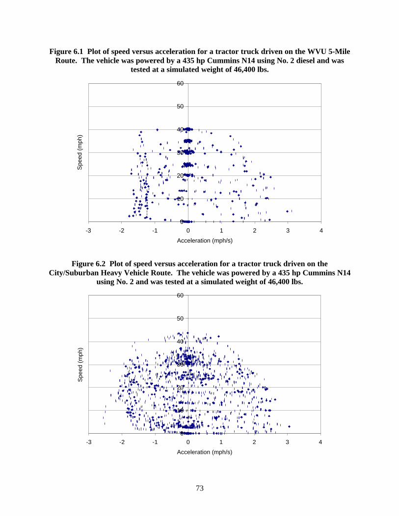
73

Figure 6.1 Plot of speed versus acceleration for a tractor truck driven on the WVU 5-MileRoute. The vehicle was powered by a 435 hp Cummins N14 using No. 2 diesel and was

tested at a simulated weight of 46,400 lbs.

0

10

20

30

40

50

60

-3 -2 -1 0 1 2 3 4


Spe

ed (

mph

)

Figure 6.2 Plot of speed versus acceleration for a tractor truck driven on theCity/Suburban Heavy Vehicle Route. The vehicle was powered by a 435 hp Cummins N14

using No. 2 and was tested at a simulated weight of 46,400 lbs.

0

10

20

30

40

50

60

-3 -2 -1 0 1 2 3 4


Spe

ed (

mph

)

74

Figure 6.3 Plot of speed versus acceleration for a tractor truck driven on Test-D. Thevehicle was powered by a 435 hp Cummins N14 using No. 2 diesel and was tested at a

simulated weight of 46,400 lbs.

0

10

20

30

40

50

60

-3 -2 -1 0 1 2 3 4


Spe

ed (

mph

)

Figure 6.4 Speed versus acceleration for a transit bus driven on the CBD cycle. Thevehicle was powered by a 275 hp DDC Series 50 using No. 2 diesel and was tested at a


0

5

10

15

20

25

-7 -5 -3 -1 1 3 5 7


Spe

ed (

mph

)

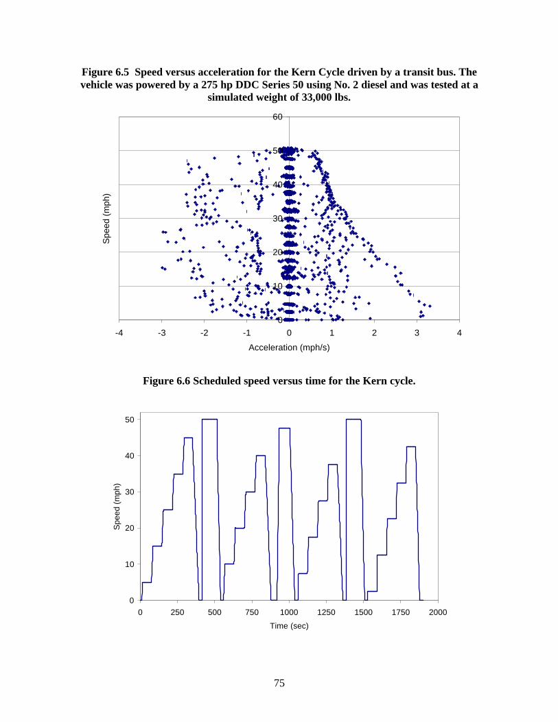
75

Figure 6.5 Speed versus acceleration for the Kern Cycle driven by a transit bus. Thevehicle was powered by a 275 hp DDC Series 50 using No. 2 diesel and was tested at a


0

10

20

30

40

50

60

-4 -3 -2 -1 0 1 2 3 4


Spe

ed (

mph

)

Figure 6.6 Scheduled speed versus time for the Kern cycle.

0

10

20

30

40

50

0 250 500 750 1000 1250 1500 1750 2000

Time (sec)

Spe

ed (

mph

)

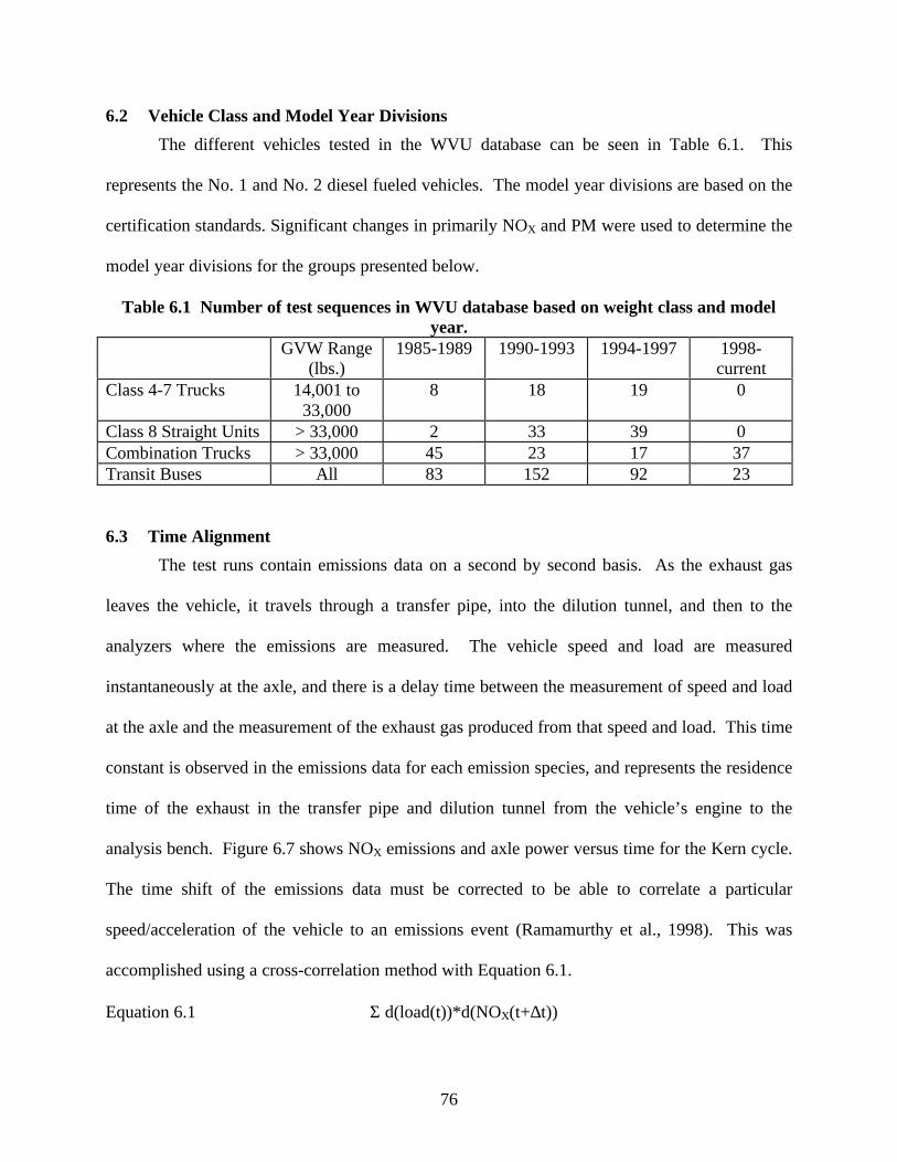
76

6.2 Vehicle Class and Model Year Divisions

The different vehicles tested in the WVU database can be seen in Table 6.1. This

represents the No. 1 and No. 2 diesel fueled vehicles. The model year divisions are based on the

certification standards. Significant changes in primarily NOX and PM were used to determine the

model year divisions for the groups presented below.

Table 6.1 Number of test sequences in WVU database based on weight class and modelyear.

GVW Range(lbs.)

1985-1989 1990-1993 1994-1997 1998-current

Class 4-7 Trucks 14,001 to33,000

8 18 19 0

Class 8 Straight Units > 33,000 2 33 39 0Combination Trucks > 33,000 45 23 17 37Transit Buses All 83 152 92 23

6.3 Time Alignment

The test runs contain emissions data on a second by second basis. As the exhaust gas

leaves the vehicle, it travels through a transfer pipe, into the dilution tunnel, and then to the

analyzers where the emissions are measured. The vehicle speed and load are measured

instantaneously at the axle, and there is a delay time between the measurement of speed and load

at the axle and the measurement of the exhaust gas produced from that speed and load. This time

constant is observed in the emissions data for each emission species, and represents the residence

time of the exhaust in the transfer pipe and dilution tunnel from the vehicle’s engine to the

analysis bench. Figure 6.7 shows NOX emissions and axle power versus time for the Kern cycle.

The time shift of the emissions data must be corrected to be able to correlate a particular

speed/acceleration of the vehicle to an emissions event (Ramamurthy et al., 1998). This was

accomplished using a cross-correlation method with Equation 6.1.

Equation 6.1 Σ d(load(t))*d(NOX(t+∆t))

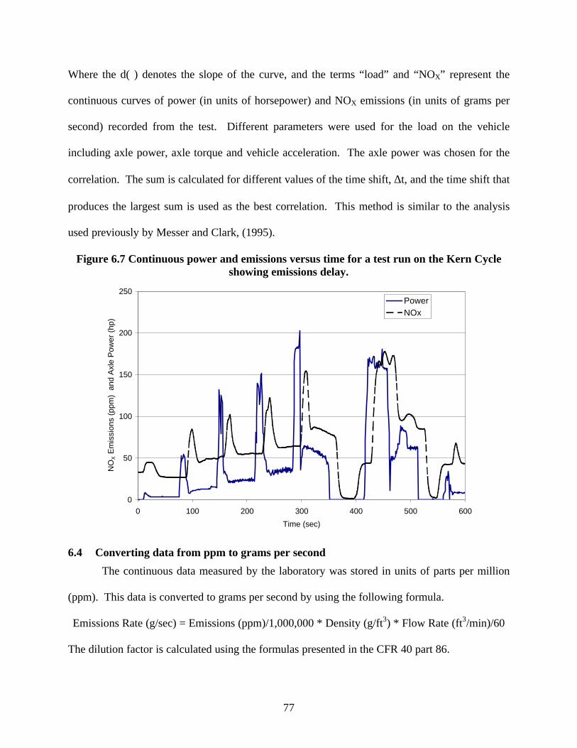
77

Where the d( ) denotes the slope of the curve, and the terms “load” and “NOX” represent the

continuous curves of power (in units of horsepower) and NOX emissions (in units of grams per

second) recorded from the test. Different parameters were used for the load on the vehicle

including axle power, axle torque and vehicle acceleration. The axle power was chosen for the

correlation. The sum is calculated for different values of the time shift, ∆t, and the time shift that

produces the largest sum is used as the best correlation. This method is similar to the analysis

used previously by Messer and Clark, (1995).

Figure 6.7 Continuous power and emissions versus time for a test run on the Kern Cycleshowing emissions delay.

0

50

100

150

200

250

0 100 200 300 400 500 600

Time (sec)

NO

X E

mis

sion

s (p

pm)

and

Axl

e P

ower

(hp

)

PowerNOx

6.4 Converting data from ppm to grams per second

The continuous data measured by the laboratory was stored in units of parts per million

(ppm). This data is converted to grams per second by using the following formula.

Emissions Rate (g/sec) = Emissions (ppm)/1,000,000 * Density (g/ft3) * Flow Rate (ft3/min)/60

The dilution factor is calculated using the formulas presented in the CFR 40 part 86.

78

6.5 Calculation of Axle Power

The database stores information other than the emissions data about the vehicle as a test

is performed. Two of these are axle angular speed and axle torque. By using these two

continuous curves, the vehicle speed in miles per hour and the axle power in horsepower were

calculated.

6.6 Proportioning PM to CO

In the absence of continuously measured particulate matter in the WVU database, an

alternate method was used. The PM is measured gravimetrically for each test run and is

presented as a composite grams per mile for the test. The continuously measured emissions are

summed for the test and also presented in grams per mile for the whole test. Taking the

composite PM value and dividing by the composite CO value created a ratio of emissions. This

ratio was then multiplied by the continuous CO data to make continuous PM data. This method

has been explored in detail by Clark, Jarrett, and Atkinson (1999). Only recently has continuous

PM data been available from the use of a Tapered Element Oscillating Microbalance (TEOM).

However, the accuracy of this data and the small amount available minimize its usefulness and it

has not been included in this project.

6.7 Speed – Acceleration Tables and Methods Used to Fill Empty Cells

The different speeds and accelerations that a heavy-duty vehicle experiences during

travel must be divided into bins so that any operating point defined by a speed value and an

acceleration value is represented by a specific bin. The emissions factor for that particular

vehicle is then placed in the appropriate bin based on the corresponding speed and acceleration

from the test data. The optimum range of values covered by each bin may vary depending on

application and the bins presented here are for an example of this method. Table 6.2 shows NOX

emissions data for 1997 transit buses grouped according to three acceleration bins and 12 speed

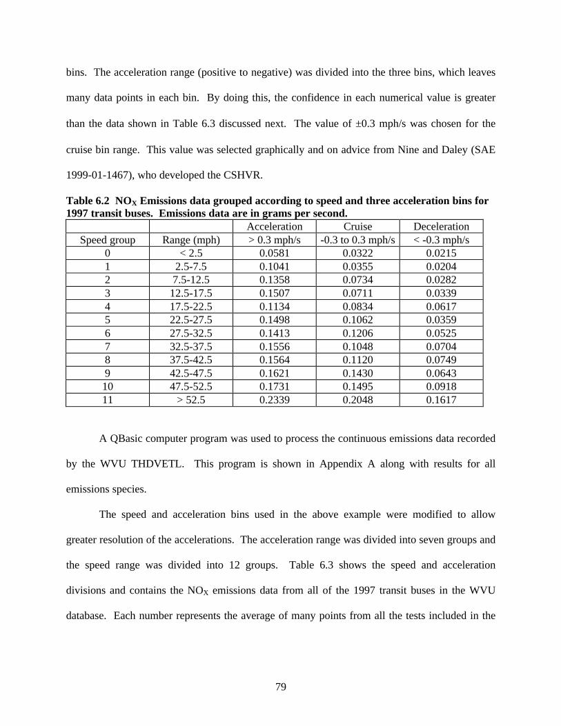
79

bins. The acceleration range (positive to negative) was divided into the three bins, which leaves

many data points in each bin. By doing this, the confidence in each numerical value is greater

than the data shown in Table 6.3 discussed next. The value of ±0.3 mph/s was chosen for the

cruise bin range. This value was selected graphically and on advice from Nine and Daley (SAE

1999-01-1467), who developed the CSHVR.

Table 6.2 NOX Emissions data grouped according to speed and three acceleration bins for1997 transit buses. Emissions data are in grams per second.

Acceleration Cruise DecelerationSpeed group Range (mph) > 0.3 mph/s -0.3 to 0.3 mph/s < -0.3 mph/s

0 < 2.5 0.0581 0.0322 0.02151 2.5-7.5 0.1041 0.0355 0.02042 7.5-12.5 0.1358 0.0734 0.02823 12.5-17.5 0.1507 0.0711 0.03394 17.5-22.5 0.1134 0.0834 0.06175 22.5-27.5 0.1498 0.1062 0.03596 27.5-32.5 0.1413 0.1206 0.05257 32.5-37.5 0.1556 0.1048 0.07048 37.5-42.5 0.1564 0.1120 0.07499 42.5-47.5 0.1621 0.1430 0.064310 47.5-52.5 0.1731 0.1495 0.091811 > 52.5 0.2339 0.2048 0.1617

A QBasic computer program was used to process the continuous emissions data recorded

by the WVU THDVETL. This program is shown in Appendix A along with results for all

emissions species.

The speed and acceleration bins used in the above example were modified to allow

greater resolution of the accelerations. The acceleration range was divided into seven groups and

the speed range was divided into 12 groups. Table 6.3 shows the speed and acceleration

divisions and contains the NOX emissions data from all of the 1997 transit buses in the WVU

database. Each number represents the average of many points from all the tests included in the

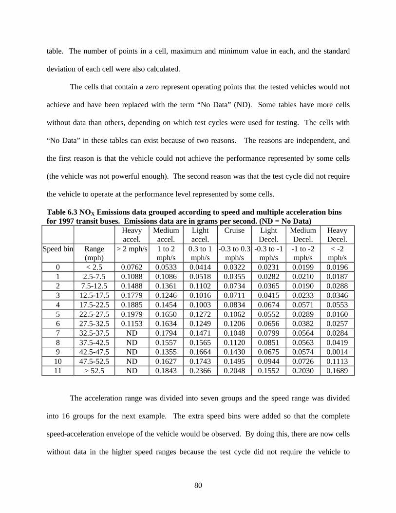
80

table. The number of points in a cell, maximum and minimum value in each, and the standard

deviation of each cell were also calculated.

The cells that contain a zero represent operating points that the tested vehicles would not

achieve and have been replaced with the term “No Data” (ND). Some tables have more cells

without data than others, depending on which test cycles were used for testing. The cells with

“No Data” in these tables can exist because of two reasons. The reasons are independent, and

the first reason is that the vehicle could not achieve the performance represented by some cells

(the vehicle was not powerful enough). The second reason was that the test cycle did not require

the vehicle to operate at the performance level represented by some cells.

Table 6.3 NOX Emissions data grouped according to speed and multiple acceleration binsfor 1997 transit buses. Emissions data are in grams per second. (ND = No Data)

Heavyaccel.

Mediumaccel.

Lightaccel.

Cruise LightDecel.

MediumDecel.

HeavyDecel.

Speed bin Range(mph)

> 2 mph/s 1 to 2mph/s

0.3 to 1mph/s

-0.3 to 0.3mph/s

-0.3 to -1mph/s

-1 to -2mph/s

< -2mph/s

0 < 2.5 0.0762 0.0533 0.0414 0.0322 0.0231 0.0199 0.01961 2.5-7.5 0.1088 0.1086 0.0518 0.0355 0.0282 0.0210 0.01872 7.5-12.5 0.1488 0.1361 0.1102 0.0734 0.0365 0.0190 0.02883 12.5-17.5 0.1779 0.1246 0.1016 0.0711 0.0415 0.0233 0.03464 17.5-22.5 0.1885 0.1454 0.1003 0.0834 0.0674 0.0571 0.05535 22.5-27.5 0.1979 0.1650 0.1272 0.1062 0.0552 0.0289 0.01606 27.5-32.5 0.1153 0.1634 0.1249 0.1206 0.0656 0.0382 0.02577 32.5-37.5 ND 0.1794 0.1471 0.1048 0.0799 0.0564 0.02848 37.5-42.5 ND 0.1557 0.1565 0.1120 0.0851 0.0563 0.04199 42.5-47.5 ND 0.1355 0.1664 0.1430 0.0675 0.0574 0.0014

10 47.5-52.5 ND 0.1627 0.1743 0.1495 0.0944 0.0726 0.111311 > 52.5 ND 0.1843 0.2366 0.2048 0.1552 0.2030 0.1689

The acceleration range was divided into seven groups and the speed range was divided

into 16 groups for the next example. The extra speed bins were added so that the complete

speed-acceleration envelope of the vehicle would be observed. By doing this, there are now cells

without data in the higher speed ranges because the test cycle did not require the vehicle to

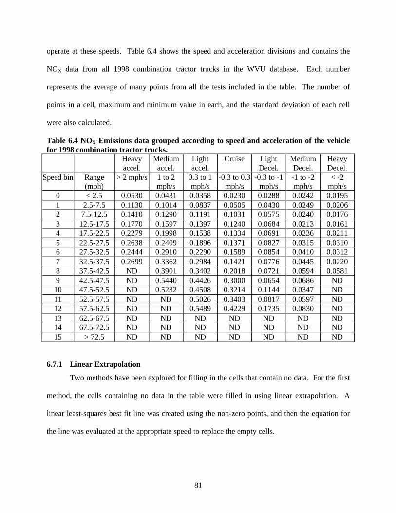
81

operate at these speeds. Table 6.4 shows the speed and acceleration divisions and contains the

NOX data from all 1998 combination tractor trucks in the WVU database. Each number

represents the average of many points from all the tests included in the table. The number of

points in a cell, maximum and minimum value in each, and the standard deviation of each cell

were also calculated.

Table 6.4 NOX Emissions data grouped according to speed and acceleration of the vehiclefor 1998 combination tractor trucks.

Heavyaccel.

Mediumaccel.

Lightaccel.

Cruise LightDecel.

MediumDecel.

HeavyDecel.

Speed bin Range(mph)

> 2 mph/s 1 to 2mph/s

0.3 to 1mph/s

-0.3 to 0.3mph/s

-0.3 to -1mph/s

-1 to -2mph/s

< -2mph/s

0 < 2.5 0.0530 0.0431 0.0358 0.0230 0.0288 0.0242 0.01951 2.5-7.5 0.1130 0.1014 0.0837 0.0505 0.0430 0.0249 0.02062 7.5-12.5 0.1410 0.1290 0.1191 0.1031 0.0575 0.0240 0.01763 12.5-17.5 0.1770 0.1597 0.1397 0.1240 0.0684 0.0213 0.01614 17.5-22.5 0.2279 0.1998 0.1538 0.1334 0.0691 0.0236 0.02115 22.5-27.5 0.2638 0.2409 0.1896 0.1371 0.0827 0.0315 0.03106 27.5-32.5 0.2444 0.2910 0.2290 0.1589 0.0854 0.0410 0.03127 32.5-37.5 0.2699 0.3362 0.2984 0.1421 0.0776 0.0445 0.02208 37.5-42.5 ND 0.3901 0.3402 0.2018 0.0721 0.0594 0.05819 42.5-47.5 ND 0.5440 0.4426 0.3000 0.0654 0.0686 ND

10 47.5-52.5 ND 0.5232 0.4508 0.3214 0.1144 0.0347 ND11 52.5-57.5 ND ND 0.5026 0.3403 0.0817 0.0597 ND12 57.5-62.5 ND ND 0.5489 0.4229 0.1735 0.0830 ND13 62.5-67.5 ND ND ND ND ND ND ND14 67.5-72.5 ND ND ND ND ND ND ND15 > 72.5 ND ND ND ND ND ND ND

6.7.1 Linear Extrapolation

Two methods have been explored for filling in the cells that contain no data. For the first

method, the cells containing no data in the table were filled in using linear extrapolation. A

linear least-squares best fit line was created using the non-zero points, and then the equation for

the line was evaluated at the appropriate speed to replace the empty cells.

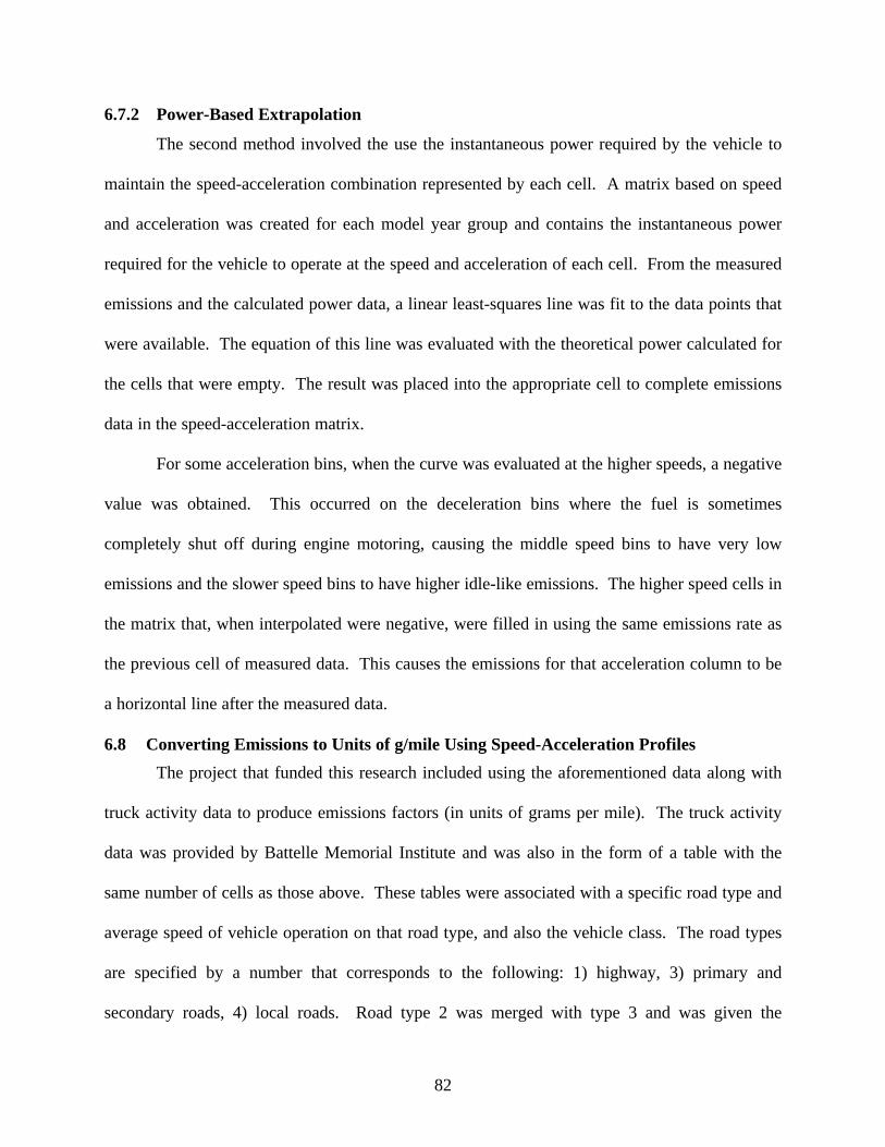
82

6.7.2 Power-Based Extrapolation

The second method involved the use the instantaneous power required by the vehicle to

maintain the speed-acceleration combination represented by each cell. A matrix based on speed

and acceleration was created for each model year group and contains the instantaneous power

required for the vehicle to operate at the speed and acceleration of each cell. From the measured

emissions and the calculated power data, a linear least-squares line was fit to the data points that

were available. The equation of this line was evaluated with the theoretical power calculated for

the cells that were empty. The result was placed into the appropriate cell to complete emissions

data in the speed-acceleration matrix.

For some acceleration bins, when the curve was evaluated at the higher speeds, a negative

value was obtained. This occurred on the deceleration bins where the fuel is sometimes

completely shut off during engine motoring, causing the middle speed bins to have very low

emissions and the slower speed bins to have higher idle-like emissions. The higher speed cells in

the matrix that, when interpolated were negative, were filled in using the same emissions rate as

the previous cell of measured data. This causes the emissions for that acceleration column to be

a horizontal line after the measured data.

6.8 Converting Emissions to Units of g/mile Using Speed-Acceleration Profiles

The project that funded this research included using the aforementioned data along with

truck activity data to produce emissions factors (in units of grams per mile). The truck activity

data was provided by Battelle Memorial Institute and was also in the form of a table with the

same number of cells as those above. These tables were associated with a specific road type and

average speed of vehicle operation on that road type, and also the vehicle class. The road types

are specified by a number that corresponds to the following: 1) highway, 3) primary and

secondary roads, 4) local roads. Road type 2 was merged with type 3 and was given the

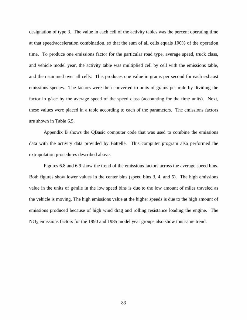
83

designation of type 3. The value in each cell of the activity tables was the percent operating time

at that speed/acceleration combination, so that the sum of all cells equals 100% of the operation

time. To produce one emissions factor for the particular road type, average speed, truck class,

and vehicle model year, the activity table was multiplied cell by cell with the emissions table,

and then summed over all cells. This produces one value in grams per second for each exhaust

emissions species. The factors were then converted to units of grams per mile by dividing the

factor in g/sec by the average speed of the speed class (accounting for the time units). Next,

these values were placed in a table according to each of the parameters. The emissions factors

are shown in Table 6.5.

Appendix B shows the QBasic computer code that was used to combine the emissions

data with the activity data provided by Battelle. This computer program also performed the

extrapolation procedures described above.

Figures 6.8 and 6.9 show the trend of the emissions factors across the average speed bins.

Both figures show lower values in the center bins (speed bins 3, 4, and 5). The high emissions

value in the units of g/mile in the low speed bins is due to the low amount of miles traveled as

the vehicle is moving. The high emissions value at the higher speeds is due to the high amount of

emissions produced because of high wind drag and rolling resistance loading the engine. The

NOX emissions factors for the 1990 and 1985 model year groups also show this same trend.

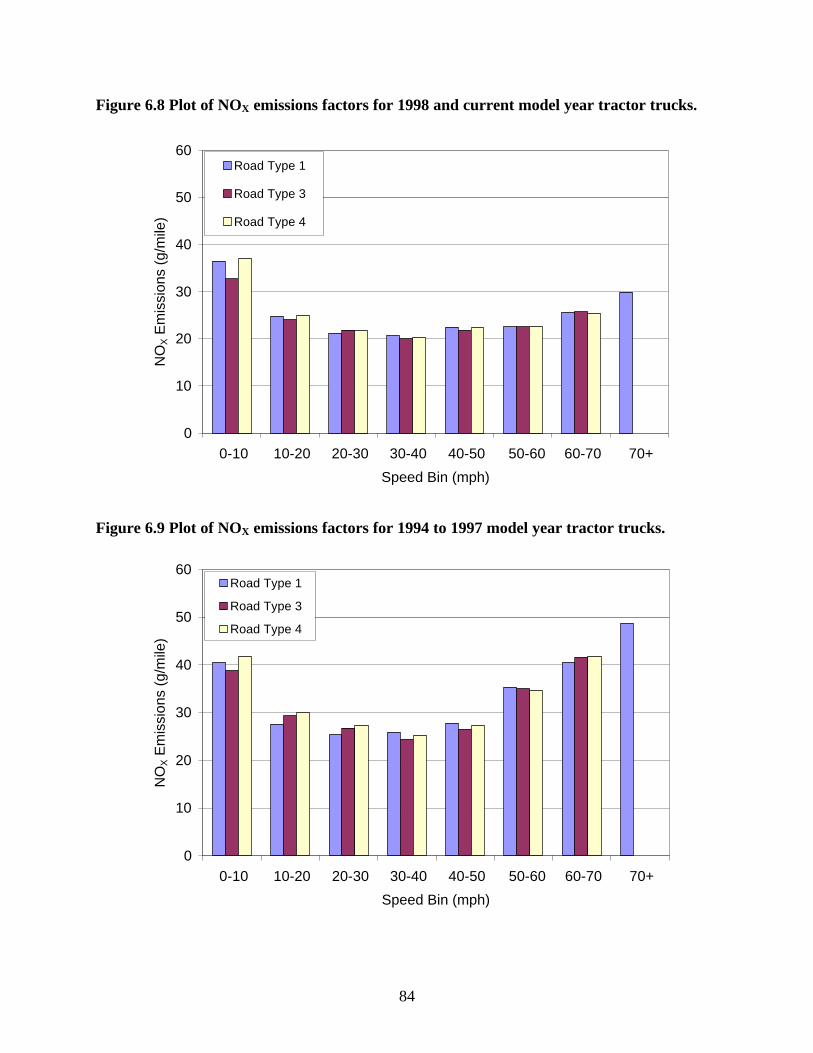
84

Figure 6.8 Plot of NOX emissions factors for 1998 and current model year tractor trucks.

0

10

20

30

40

50

60

0-10 10-20 20-30 30-40 40-50 50-60 60-70 70+

Speed Bin (mph)

NO

X E

mis

sion

s (g

/mile

)Road Type 1

Road Type 3

Road Type 4

Figure 6.9 Plot of NOX emissions factors for 1994 to 1997 model year tractor trucks.

0

10

20

30

40

50

60

0-10 10-20 20-30 30-40 40-50 50-60 60-70 70+

Speed Bin (mph)

NO

X E

mis

sion

s (g

/mile

)

Road Type 1

Road Type 3

Road Type 4

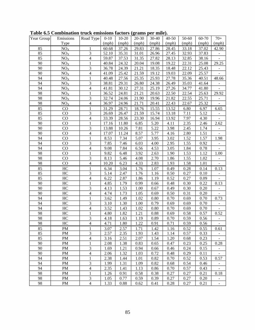
85

Table 6.5 Combination truck emissions factors (grams per mile).Year Group Emissions

TypeRoad Type 0-10

(mph)10-20(mph)

20-30(mph)

30-40(mph)

40-50(mph)

50-60(mph)

60-70(mph)

70+(mph)

85 NOX 1 60.68 37.26 29.83 27.86 28.45 33.18 37.02 42.9085 NOX 3 52.10 35.31 31.01 26.96 27.45 32.93 37.83 -85 NOX 4 59.87 37.53 31.35 27.82 28.13 32.85 38.16 -90 NOX 1 40.84 24.32 20.04 19.08 19.22 22.31 25.08 29.2590 NOX 3 36.78 24.39 21.21 18.35 18.48 22.12 25.43 -90 NOX 4 41.09 25.42 21.59 19.12 19.03 22.09 25.57 -94 NOX 1 40.48 27.56 25.35 25.93 27.78 35.36 40.51 48.6694 NOX 3 38.81 29.31 26.80 24.38 26.49 35.03 41.64 -94 NOX 4 41.81 30.12 27.31 25.19 27.26 34.77 41.80 -98 NOX 1 36.52 24.81 21.21 20.63 22.50 22.54 25.63 29.9298 NOX 3 32.74 24.06 21.90 19.96 21.82 22.55 25.71 -98 NOX 4 36.97 24.96 21.71 20.41 22.43 22.67 25.32 -85 CO 1 31.29 28.71 18.76 15.55 13.52 6.80 6.97 6.6585 CO 3 26.69 26.47 21.59 15.74 13.18 7.11 5.12 -85 CO 4 33.39 28.56 23.30 16.94 13.92 7.97 4.30 -90 CO 1 17.16 11.80 6.85 5.20 4.11 2.35 2.46 2.6290 CO 3 13.88 10.26 7.81 5.22 3.98 2.45 1.74 -90 CO 4 17.07 11.24 8.57 5.77 4.16 2.80 1.51 -94 CO 1 8.53 7.34 5.07 3.95 3.02 1.52 1.57 1.9894 CO 3 7.85 7.46 6.03 4.00 2.95 1.55 0.92 -94 CO 4 9.08 7.84 6.56 4.53 3.05 1.84 0.78 -98 CO 1 9.82 6.48 3.92 2.63 1.90 1.53 1.12 1.0098 CO 3 8.13 5.46 4.08 2.70 1.86 1.55 1.02 -98 CO 4 10.20 6.23 4.33 2.83 1.93 1.58 1.01 -85 HC 1 6.34 3.04 1.76 1.07 0.49 0.28 0.14 0.1385 HC 3 5.14 2.47 1.76 1.16 0.50 0.27 0.10 -85 HC 4 6.22 2.87 1.86 1.19 0.52 0.27 0.09 -90 HC 1 4.85 1.79 0.99 0.66 0.48 0.30 0.22 0.1390 HC 3 4.13 1.53 1.00 0.67 0.49 0.30 0.20 -90 HC 4 4.74 1.73 1.05 0.69 0.50 0.31 0.20 -94 HC 1 3.62 1.49 1.02 0.80 0.70 0.69 0.70 0.7394 HC 3 3.10 1.30 1.00 0.79 0.69 0.69 0.70 -94 HC 4 3.52 1.43 1.02 0.80 0.70 0.69 0.70 -98 HC 1 4.80 1.82 1.21 0.88 0.69 0.58 0.57 0.5298 HC 3 4.18 1.63 1.19 0.89 0.70 0.59 0.56 -98 HC 4 4.71 1.80 1.22 0.91 0.71 0.59 0.56 -85 PM 1 3.07 2.57 1.71 1.42 1.16 0.52 0.55 0.6185 PM 3 2.57 2.35 1.93 1.43 1.14 0.57 0.33 -85 PM 4 3.16 2.51 2.07 1.54 1.20 0.68 0.23 -90 PM 1 2.08 1.38 0.83 0.65 0.47 0.23 0.25 0.2890 PM 3 1.69 1.21 0.94 0.66 0.46 0.24 0.15 -90 PM 4 2.06 1.32 1.03 0.72 0.48 0.29 0.11 -94 PM 1 2.38 1.44 1.01 0.82 0.70 0.52 0.53 0.5794 PM 3 1.99 1.31 1.09 0.82 0.68 0.54 0.46 -94 PM 4 2.35 1.41 1.13 0.86 0.70 0.57 0.43 -98 PM 1 1.26 0.91 0.58 0.38 0.27 0.27 0.21 0.1898 PM 3 1.05 0.77 0.59 0.39 0.27 0.27 0.20 -98 PM 4 1.33 0.88 0.62 0.41 0.28 0.27 0.21 -

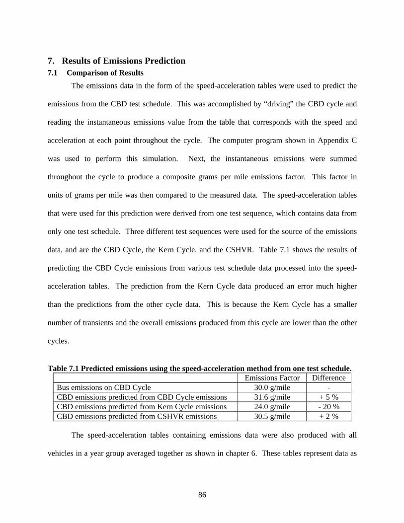
86

7. Results of Emissions Prediction7.1 Comparison of Results

The emissions data in the form of the speed-acceleration tables were used to predict the

emissions from the CBD test schedule. This was accomplished by “driving” the CBD cycle and

reading the instantaneous emissions value from the table that corresponds with the speed and

acceleration at each point throughout the cycle. The computer program shown in Appendix C

was used to perform this simulation. Next, the instantaneous emissions were summed

throughout the cycle to produce a composite grams per mile emissions factor. This factor in

units of grams per mile was then compared to the measured data. The speed-acceleration tables

that were used for this prediction were derived from one test sequence, which contains data from

only one test schedule. Three different test sequences were used for the source of the emissions

data, and are the CBD Cycle, the Kern Cycle, and the CSHVR. Table 7.1 shows the results of

predicting the CBD Cycle emissions from various test schedule data processed into the speed-

acceleration tables. The prediction from the Kern Cycle data produced an error much higher

than the predictions from the other cycle data. This is because the Kern Cycle has a smaller

number of transients and the overall emissions produced from this cycle are lower than the other

cycles.

Table 7.1 Predicted emissions using the speed-acceleration method from one test schedule.Emissions Factor Difference

Bus emissions on CBD Cycle 30.0 g/mile -CBD emissions predicted from CBD Cycle emissions 31.6 g/mile + 5 %CBD emissions predicted from Kern Cycle emissions 24.0 g/mile - 20 %CBD emissions predicted from CSHVR emissions 30.5 g/mile + 2 %

The speed-acceleration tables containing emissions data were also produced with all

vehicles in a year group averaged together as shown in chapter 6. These tables represent data as

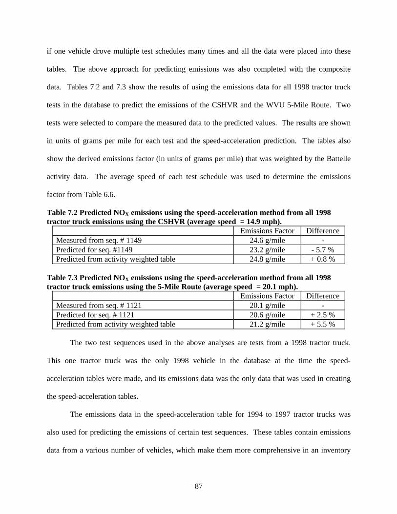
87

if one vehicle drove multiple test schedules many times and all the data were placed into these

tables. The above approach for predicting emissions was also completed with the composite

data. Tables 7.2 and 7.3 show the results of using the emissions data for all 1998 tractor truck

tests in the database to predict the emissions of the CSHVR and the WVU 5-Mile Route. Two

tests were selected to compare the measured data to the predicted values. The results are shown

in units of grams per mile for each test and the speed-acceleration prediction. The tables also

show the derived emissions factor (in units of grams per mile) that was weighted by the Battelle

activity data. The average speed of each test schedule was used to determine the emissions

factor from Table 6.6.

Table 7.2 Predicted NOX emissions using the speed-acceleration method from all 1998tractor truck emissions using the CSHVR (average speed = 14.9 mph).

Emissions Factor DifferenceMeasured from seq. # 1149 24.6 g/mile -Predicted for seq. #1149 23.2 g/mile - 5.7 %Predicted from activity weighted table 24.8 g/mile + 0.8 %

Table 7.3 Predicted NOX emissions using the speed-acceleration method from all 1998tractor truck emissions using the 5-Mile Route (average speed = 20.1 mph).

Emissions Factor DifferenceMeasured from seq. # 1121 20.1 g/mile -Predicted for seq. # 1121 20.6 g/mile + 2.5 %Predicted from activity weighted table 21.2 g/mile + 5.5 %

The two test sequences used in the above analyses are tests from a 1998 tractor truck.

This one tractor truck was the only 1998 vehicle in the database at the time the speed-

acceleration tables were made, and its emissions data was the only data that was used in creating

the speed-acceleration tables.

The emissions data in the speed-acceleration table for 1994 to 1997 tractor trucks was

also used for predicting the emissions of certain test sequences. These tables contain emissions

data from a various number of vehicles, which make them more comprehensive in an inventory

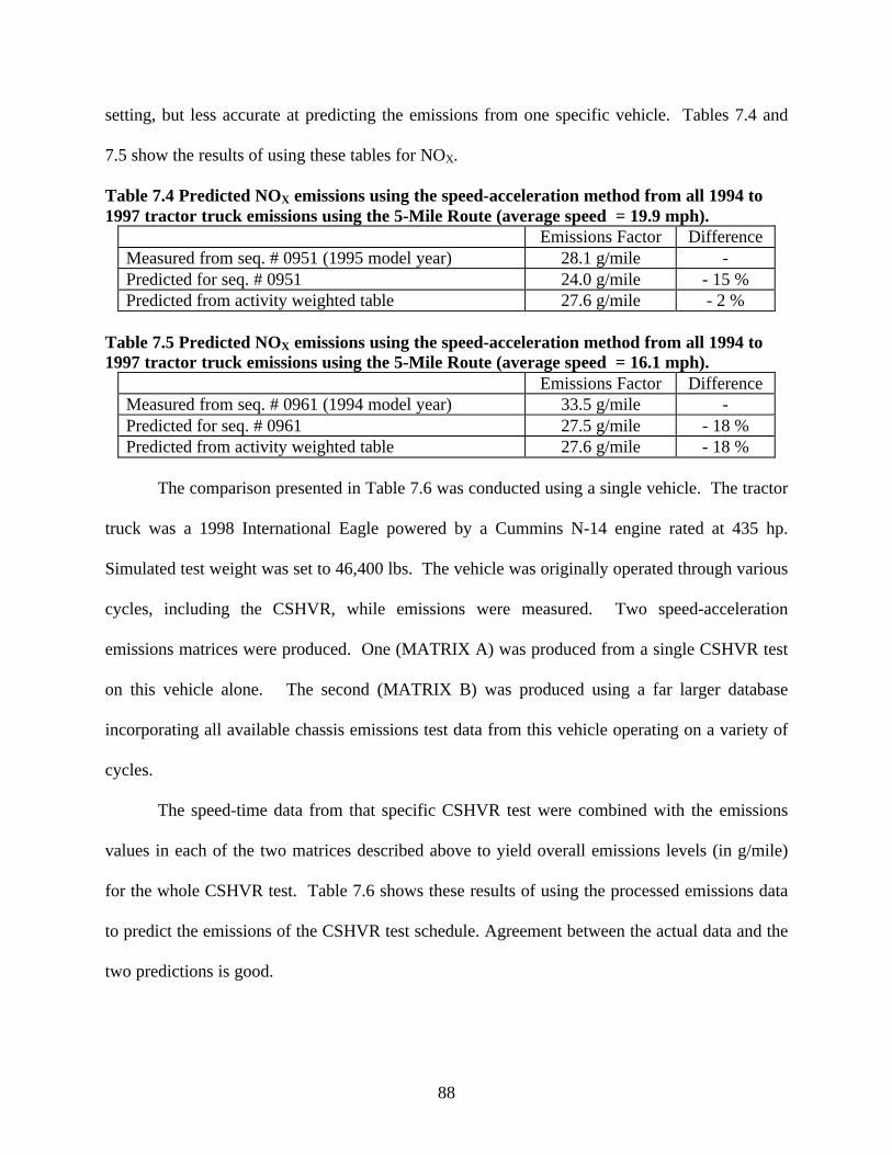
88

setting, but less accurate at predicting the emissions from one specific vehicle. Tables 7.4 and

7.5 show the results of using these tables for NOX.


Emissions Factor DifferenceMeasured from seq. # 0951 (1995 model year) 28.1 g/mile -Predicted for seq. # 0951 24.0 g/mile - 15 %Predicted from activity weighted table 27.6 g/mile - 2 %


Emissions Factor DifferenceMeasured from seq. # 0961 (1994 model year) 33.5 g/mile -Predicted for seq. # 0961 27.5 g/mile - 18 %Predicted from activity weighted table 27.6 g/mile - 18 %

The comparison presented in Table 7.6 was conducted using a single vehicle. The tractor

truck was a 1998 International Eagle powered by a Cummins N-14 engine rated at 435 hp.

Simulated test weight was set to 46,400 lbs. The vehicle was originally operated through various

cycles, including the CSHVR, while emissions were measured. Two speed-acceleration

emissions matrices were produced. One (MATRIX A) was produced from a single CSHVR test

on this vehicle alone. The second (MATRIX B) was produced using a far larger database

incorporating all available chassis emissions test data from this vehicle operating on a variety of

cycles.

The speed-time data from that specific CSHVR test were combined with the emissions

values in each of the two matrices described above to yield overall emissions levels (in g/mile)

for the whole CSHVR test. Table 7.6 shows these results of using the processed emissions data

to predict the emissions of the CSHVR test schedule. Agreement between the actual data and the

two predictions is good.

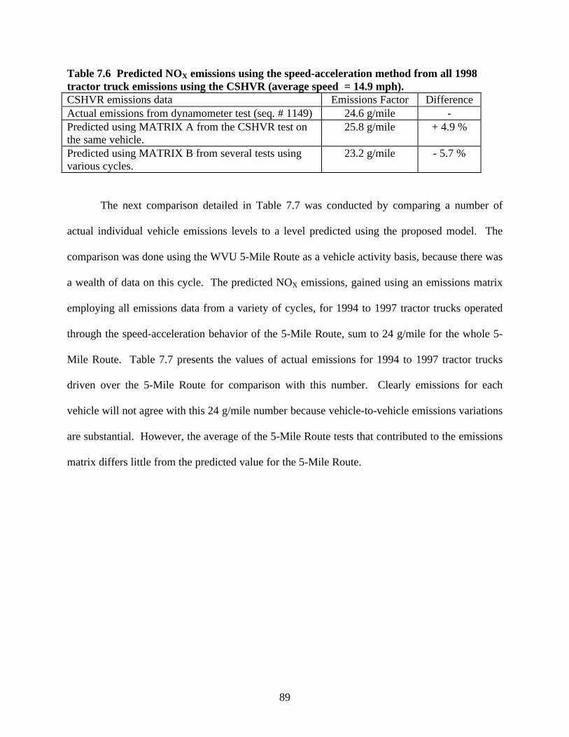
89

Table 7.6 Predicted NOX emissions using the speed-acceleration method from all 1998tractor truck emissions using the CSHVR (average speed = 14.9 mph).CSHVR emissions data Emissions Factor DifferenceActual emissions from dynamometer test (seq. # 1149) 24.6 g/mile -Predicted using MATRIX A from the CSHVR test onthe same vehicle.

25.8 g/mile + 4.9 %

Predicted using MATRIX B from several tests usingvarious cycles.

23.2 g/mile - 5.7 %

The next comparison detailed in Table 7.7 was conducted by comparing a number of

actual individual vehicle emissions levels to a level predicted using the proposed model. The

comparison was done using the WVU 5-Mile Route as a vehicle activity basis, because there was

a wealth of data on this cycle. The predicted NOX emissions, gained using an emissions matrix

employing all emissions data from a variety of cycles, for 1994 to 1997 tractor trucks operated

through the speed-acceleration behavior of the 5-Mile Route, sum to 24 g/mile for the whole 5-

Mile Route. Table 7.7 presents the values of actual emissions for 1994 to 1997 tractor trucks

driven over the 5-Mile Route for comparison with this number. Clearly emissions for each

vehicle will not agree with this 24 g/mile number because vehicle-to-vehicle emissions variations

are substantial. However, the average of the 5-Mile Route tests that contributed to the emissions

matrix differs little from the predicted value for the 5-Mile Route.

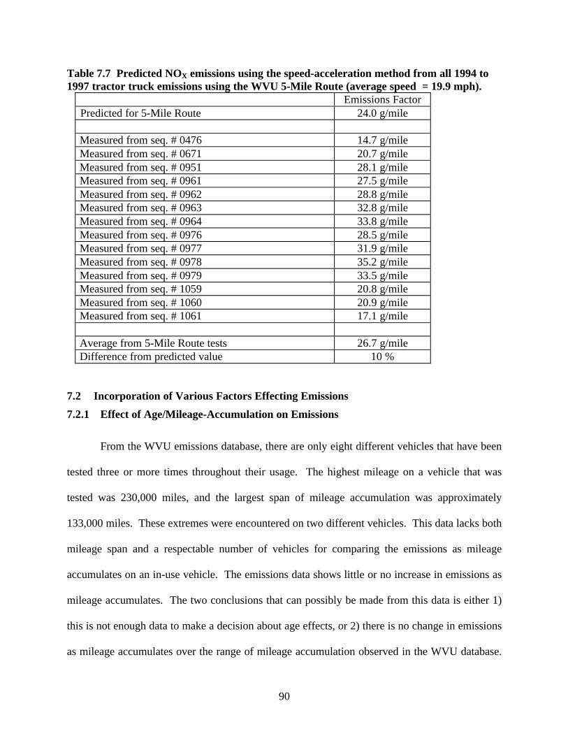
90

Table 7.7 Predicted NOX emissions using the speed-acceleration method from all 1994 to1997 tractor truck emissions using the WVU 5-Mile Route (average speed = 19.9 mph).

Emissions FactorPredicted for 5-Mile Route 24.0 g/mile

Measured from seq. # 0476 14.7 g/mile Measured from seq. # 0671 20.7 g/mile Measured from seq. # 0951 28.1 g/mile Measured from seq. # 0961 27.5 g/mile Measured from seq. # 0962 28.8 g/mile Measured from seq. # 0963 32.8 g/mile Measured from seq. # 0964 33.8 g/mile Measured from seq. # 0976 28.5 g/mile Measured from seq. # 0977 31.9 g/mile Measured from seq. # 0978 35.2 g/mile Measured from seq. # 0979 33.5 g/mile Measured from seq. # 1059 20.8 g/mile Measured from seq. # 1060 20.9 g/mile Measured from seq. # 1061 17.1 g/mile

Average from 5-Mile Route tests 26.7 g/mile Difference from predicted value 10 %

7.2 Incorporation of Various Factors Effecting Emissions

7.2.1 Effect of Age/Mileage-Accumulation on Emissions

From the WVU emissions database, there are only eight different vehicles that have been

tested three or more times throughout their usage. The highest mileage on a vehicle that was

tested was 230,000 miles, and the largest span of mileage accumulation was approximately

133,000 miles. These extremes were encountered on two different vehicles. This data lacks both

mileage span and a respectable number of vehicles for comparing the emissions as mileage

accumulates on an in-use vehicle. The emissions data shows little or no increase in emissions as

mileage accumulates. The two conclusions that can possibly be made from this data is either 1)

this is not enough data to make a decision about age effects, or 2) there is no change in emissions

as mileage accumulates over the range of mileage accumulation observed in the WVU database.

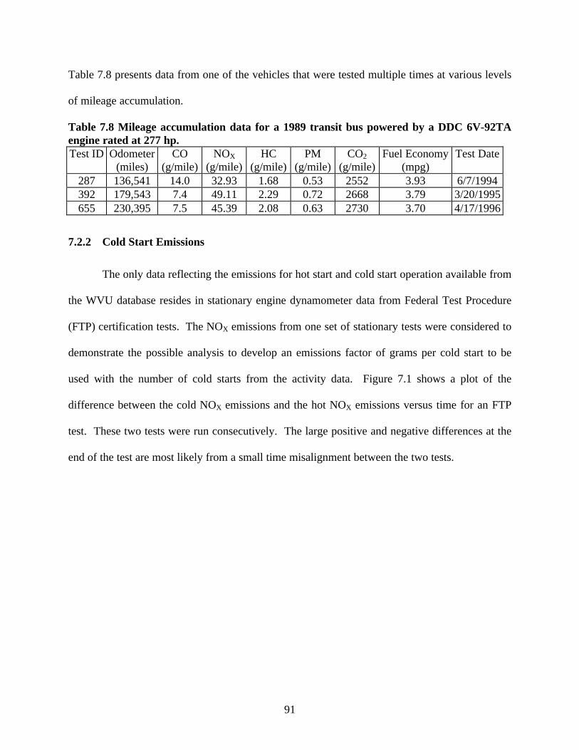
91

Table 7.8 presents data from one of the vehicles that were tested multiple times at various levels

of mileage accumulation.

Table 7.8 Mileage accumulation data for a 1989 transit bus powered by a DDC 6V-92TAengine rated at 277 hp.Test ID Odometer

(miles)CO

(g/mile)NOX

(g/mile)HC

(g/mile)PM

(g/mile)CO2

(g/mile)Fuel Economy

(mpg)Test Date

287 136,541 14.0 32.93 1.68 0.53 2552 3.93 6/7/1994392 179,543 7.4 49.11 2.29 0.72 2668 3.79 3/20/1995655 230,395 7.5 45.39 2.08 0.63 2730 3.70 4/17/1996

7.2.2 Cold Start Emissions

The only data reflecting the emissions for hot start and cold start operation available from

the WVU database resides in stationary engine dynamometer data from Federal Test Procedure

(FTP) certification tests. The NOX emissions from one set of stationary tests were considered to

demonstrate the possible analysis to develop an emissions factor of grams per cold start to be

used with the number of cold starts from the activity data. Figure 7.1 shows a plot of the

difference between the cold NOX emissions and the hot NOX emissions versus time for an FTP

test. These two tests were run consecutively. The large positive and negative differences at the

end of the test are most likely from a small time misalignment between the two tests.

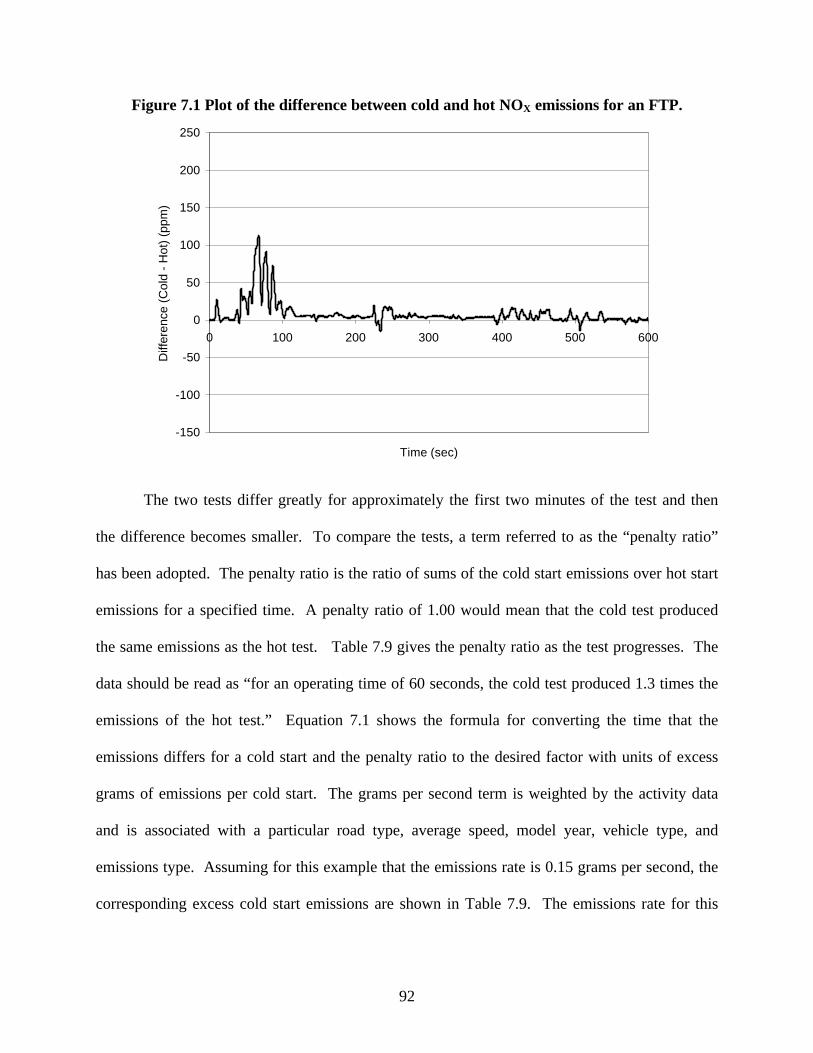
92

Figure 7.1 Plot of the difference between cold and hot NOX emissions for an FTP.

-150

-100

-50

0

50

100

150

200

250

0 100 200 300 400 500 600

Time (sec)

Diff

eren

ce (

Col

d -

Hot

) (p

pm)

The two tests differ greatly for approximately the first two minutes of the test and then

the difference becomes smaller. To compare the tests, a term referred to as the “penalty ratio”

has been adopted. The penalty ratio is the ratio of sums of the cold start emissions over hot start

emissions for a specified time. A penalty ratio of 1.00 would mean that the cold test produced

the same emissions as the hot test. Table 7.9 gives the penalty ratio as the test progresses. The

data should be read as “for an operating time of 60 seconds, the cold test produced 1.3 times the

emissions of the hot test.” Equation 7.1 shows the formula for converting the time that the

emissions differs for a cold start and the penalty ratio to the desired factor with units of excess

grams of emissions per cold start. The grams per second term is weighted by the activity data

and is associated with a particular road type, average speed, model year, vehicle type, and

emissions type. Assuming for this example that the emissions rate is 0.15 grams per second, the

corresponding excess cold start emissions are shown in Table 7.9. The emissions rate for this

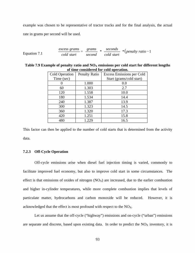
93

example was chosen to be representative of tractor trucks and for the final analysis, the actual

rate in grams per second will be used.

Equation 7.1 ( )1** −

= ratiopenalty

startcold

seconds

second

grams

startcold

gramsexcess

Table 7.9 Example of penalty ratio and NOX emissions per cold start for different lengthsof time considered for cold operation.

Cold OperationTime (sec)

Penalty Ratio Excess Emissions per ColdStart (grams/cold start)

0 1.000 0.060 1.303 2.7

120 1.558 10.0180 1.534 14.4240 1.387 13.9300 1.323 14.5360 1.320 17.3420 1.251 15.8480 1.229 16.5

This factor can then be applied to the number of cold starts that is determined from the activity

data.

7.2.3 Off-Cycle Operation

Off-cycle emissions arise when diesel fuel injection timing is varied, commonly to

facilitate improved fuel economy, but also to improve cold start in some circumstances. The

effect is that emissions of oxides of nitrogen (NOX) are increased, due to the earlier combustion

and higher in-cylinder temperatures, while more complete combustion implies that levels of

particulate matter, hydrocarbons and carbon monoxide will be reduced. However, it is

acknowledged that the effect is most profound with respect to the NOX.

Let us assume that the off-cycle (“highway”) emissions and on-cycle (“urban”) emissions

are separate and discrete, based upon existing data. In order to predict the NOX inventory, it is

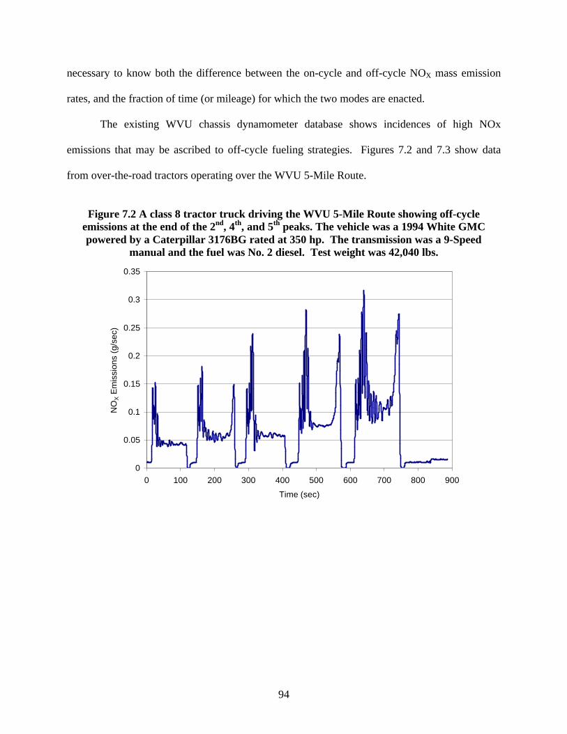
94

necessary to know both the difference between the on-cycle and off-cycle NOX mass emission

rates, and the fraction of time (or mileage) for which the two modes are enacted.

The existing WVU chassis dynamometer database shows incidences of high NOx

emissions that may be ascribed to off-cycle fueling strategies. Figures 7.2 and 7.3 show data

from over-the-road tractors operating over the WVU 5-Mile Route.

Figure 7.2 A class 8 tractor truck driving the WVU 5-Mile Route showing off-cycleemissions at the end of the 2nd, 4th, and 5th peaks. The vehicle was a 1994 White GMCpowered by a Caterpillar 3176BG rated at 350 hp. The transmission was a 9-Speed

manual and the fuel was No. 2 diesel. Test weight was 42,040 lbs.

0

0.05

0.1

0.15

0.2

0.25

0.3

0.35

0 100 200 300 400 500 600 700 800 900

Time (sec)

NO

X E

mis

sion

s (g

/sec

)

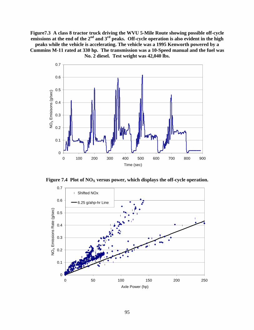
95

Figure7.3 A class 8 tractor truck driving the WVU 5-Mile Route showing possible off-cycleemissions at the end of the 2nd and 3rd peaks. Off-cycle operation is also evident in the high

peaks while the vehicle is accelerating. The vehicle was a 1995 Kenworth powered by aCummins M-11 rated at 330 hp. The transmission was a 10-Speed manual and the fuel was

No. 2 diesel. Test weight was 42,040 lbs.

0

0.1

0.2

0.3

0.4

0.5

0.6

0.7

0 100 200 300 400 500 600 700 800 900

Time (sec)

NO

X E

mis

ison

s (g

/sec

)

Figure 7.4 Plot of NOX versus power, which displays the off-cycle operation.

0

0.1

0.2

0.3

0.4

0.5

0.6

0.7

0 50 100 150 200 250

Axle Power (hp)

NO

X E

mis

sion

s R

ate

(g/s

ec)

Shifted NOx

6.25 g/ahp-hr Line

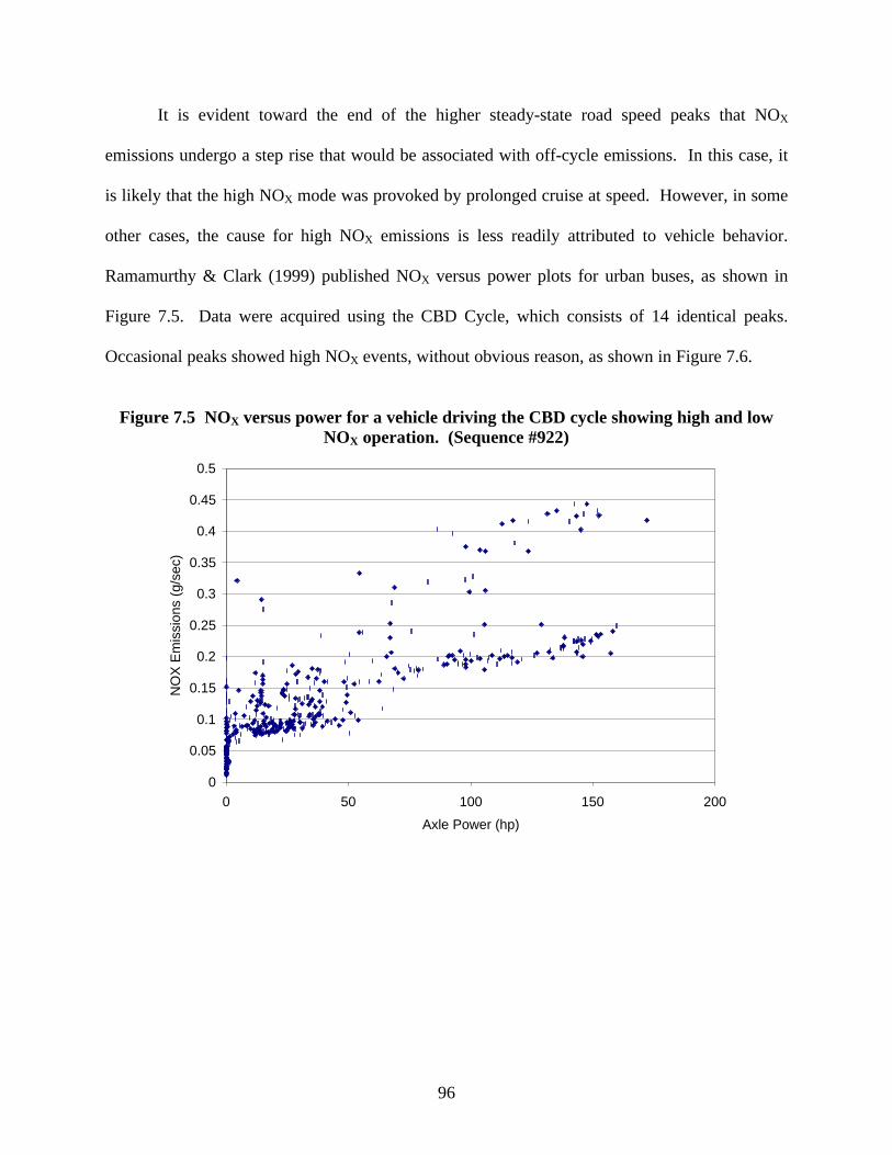
96

It is evident toward the end of the higher steady-state road speed peaks that NOX

emissions undergo a step rise that would be associated with off-cycle emissions. In this case, it

is likely that the high NOX mode was provoked by prolonged cruise at speed. However, in some

other cases, the cause for high NOX emissions is less readily attributed to vehicle behavior.

Ramamurthy & Clark (1999) published NOX versus power plots for urban buses, as shown in

Figure 7.5. Data were acquired using the CBD Cycle, which consists of 14 identical peaks.

Occasional peaks showed high NOX events, without obvious reason, as shown in Figure 7.6.

Figure 7.5 NOX versus power for a vehicle driving the CBD cycle showing high and lowNOX operation. (Sequence #922)

0

0.05

0.1

0.15

0.2

0.25

0.3

0.35

0.4

0.45

0.5

0 50 100 150 200

Axle Power (hp)

NO

X E

mis

sion

s (g

/sec

)

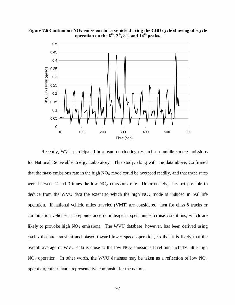
97

Figure 7.6 Continuous NOX emissions for a vehicle driving the CBD cycle showing off-cycleoperation on the 6th, 7th, 8th, and 14th peaks.

0

0.05

0.1

0.15

0.2

0.25

0.3

0.35

0.4

0.45

0.5

0 100 200 300 400 500 600

Time (sec)

NO

X E

mis

sion

s (g

/sec

)

Recently, WVU participated in a team conducting research on mobile source emissions

for National Renewable Energy Laboratory. This study, along with the data above, confirmed

that the mass emissions rate in the high NOX mode could be accessed readily, and that these rates

were between 2 and 3 times the low NOX emissions rate. Unfortunately, it is not possible to

deduce from the WVU data the extent to which the high NOX mode is induced in real life

operation. If national vehicle miles traveled (VMT) are considered, then for class 8 trucks or

combination vehciles, a preponderance of mileage is spent under cruise conditions, which are

likely to provoke high NOX emissions. The WVU database, however, has been derived using

cycles that are transient and biased toward lower speed operation, so that it is likely that the

overall average of WVU data is close to the low NOX emissions level and includes little high

NOX operation. In other words, the WVU database may be taken as a reflection of low NOX

operation, rather than a representative composite for the nation.

98

7.3 Conclusions and Recommendations

The analyses in Chapter four give an indication of the relative effects of certain variables

on the exhaust emissions of chassis-based testing. Section 4.9 gives a summary of the factors.

These factors cause inaccuracies in the use of chassis emissions data for inventory and

prediction.

Chapter five reviews different methods that can be used to develop emissions factors in

grams per mile for inventory purposes. The current method used by the EPA and CARB uses

emissions information from engine testing on FTP test cycle. The only influence of vehicle

activity present in this method is through the fuel economy values used to convert the engine

data to grams per mile of emissions. The fuel economy value is an average of fuel economies

from various driving conditions and different vehicles. This cycle-dependency and lack of

varying fuel economy limits the variability of the method. The method chosen for this analysis

includes emissions information from many different chassis cycles, and some of these cycles

have been developed from recent activity data and are meant to accurately represent the activity

that in-use vehicles are experiencing. Also, the off-cycle emissions modes of modern

electronically controlled engines are explored in the chassis testing and, by design do not occur

on an FTP engine test.

The speed-acceleration method of predicting emissions presented in chapter six shows

acceptable results when compared to measured chassis emissions in units of grams per mile.

Comparisons of the predicted values were made in chapter seven both before and after the

weighting by the activity data. The error of the predicted values was less than 20 % when

compared to measured data.

Algorithms used by the engine manufacturers to implement the advanced timing strategy

are not in the public domain, so that a simulation approach cannot be used to infer the incidence

99

or fraction of high NOX operation. It is suggested that further research will be needed to shed

light on the incidence of high NOX operation, in the following way. Representative vehicles with

electronic engine management should be procured and exercised on a chassis dynamometer for

long periods of time, using target speed-time traces selected statistically from in-use truck

activity. Emissions measured from the vehicles would provide not only composite emissions

factors representative of real use with low and high NOX operation, but would also provide

information on the fraction of time spent in a high NOX mode. This can be assessed by

monitoring real-time NOX/power and NOX/CO2 ratios for the subject vehicles. These ratios will

readily reveal the binary strategy. Also, runs of this kind would richen the overall database for

an inventory study and would provide an opportunity to log real-time particulate matter (PM)

emissions using a Tapered Element Oscillating Microbalance (TEOM). There has been little

discussion of the effects of elimination of advanced timing strategies on PM production, and no

comprehensive data exist to date to quantify the effect.

100

References

Avallone, E.A., and Baumeister, T., (eds.), "Marks' Standard Handbook for MechanicalEngineers, Tenth Edition." McGraw-Hill, New York, New York, 1996.

Bach, E., Zikoridse, G., Sandig, R., Lemaire, J., Mustel, W., Naschke, W., Bestenreiner, G., andBrück, R., "Combination of Different Regeneration Methods for Diesel Particulate Traps," SAE980541, 1998.

Bata, R., Yacoub, Y., Wang, W., and Lyons, D., "Heavy-Duty Testing Cycles: Survey andComparison." SAE 942263, 1994.

Brown, S.J., "An Experimental Investigation of Affordable Alternative Fuel and ExhaustAftertreatment Options for Urban Buses," Trucks and Buses, the results of real-world emissionstesting, Millbrook Proving Ground Seminar Proceedings, 1997.

Clark, N.N., and Lyons, D.W., "Class 8 Truck Emissions Testing; Effects of Test Cycles andData of Biodiesel Operation," ASAE Annual International Meeting, Orlando, FL, ASAE 986082,1998.

Clark, N.N., and Lyons, D.W., "Emissions from CNG and Diesel Refuse Haulers Using SixEngine Types in New York City," Seventh CRC On-Road Vehicle Emissions Workshop, SanDiego, April 1997, pp. 5-49 to 5-64.

Clark, N.N., and McKain, D.L., "Transient Chassis Cycles for Heavy-Duty Trucks andTractors," Int. Jour. Of Vehicle Design (Heavy Vehicle Systems), Vol.2, No.2, 1995, pp.143-159.

Clark, N.N., Atkinson, C.M., Thompson, G.J., Nine, R.D., "Transient Emissions Comparisons ofAlternative Compression Ignition Fuels," SAE 1999-01-1117, 1999.

Clark, N.N., Jarrett, R.P., and Atkinson, C.M., “Field Measurements of Particulate MatterEmissions, Carbon Monoxide, and Exhaust Opacity from Heavy-Duty Diesel Vehicles,” Journalof the Air and Waste Management Association, Vol. 49, 1999, pp. 76-84.

Clark, N.N., Lyons, D.W., Bata, R.M., Gautam, M., Wang, W.G., Norton, P., and Chandler, K.,"Natural Gas and Diesel Transit Bus Emissions: Review and Recent Data," SAE 973203, 1997.

Clark, N.N., McKain, D.L., Messer, J.T., and Lyons, D.W., "Chassis Test Cycles for AssessingEmissions from Heavy-Duty Trucks," Fuels and Lubricants Conference, Baltimore, MD, SAE941946, 1994.

Clark, N.N., Messer, D.J., Mckain, D.L., Wang, W.G., Bata, R.M., Gautam, M., and Lyons,D.W., "Use of the West Virginia University Truck Test Cycle to Evaluate Emissions from Class8 Trucks." SAE 951016, 1995.

101

Clark, N.N., Nine, R.D., Daley, J.J., and Atkinson, C.M., "Development of a Heavy-DutyChassis Dynamometer Driving Route, Phase I Report," 1998b.

Clark, N.N., Daley, J.J., Nine, R.D., and Atkinson, C.M., “Application of the New City-Suburban Heavy Vehicle Route (CSHVR) to Truck Emissions Characterization.” SAE 1999-01-1467, 1999.

Coburn, T., "Statistical Analysis of Particulate Matter Emissions from Light-Duty and Heavy-Duty Diesel Vehicles," NREL/TP-540-224942, July 1998.

Code of Federal Regulations, Title 40, Part 86, Subpart M, "EPA Urban Dynamometer DrivingSchedule for Heavy-Duty Engines," U.S. Government Printing Office, 1996.

Code of Federal Regulations, Title 40, Part 86, Subpart N, "Protection of the Environment,"U.S. Government Printing Office, 1996.

Diezman, H.E. and Warner-Selph, M.A., "Comparison of Emissions from Heavy-Duty Enginesand Vehicles During Transient Operation," ASME Paper 85-DGP-10, Energy Sources andTechnology Conference, Dallas, TX, 1985.

EPA Document, "Emissions Standards reference Guide for Heavy-Duty and Nonroad Engines,"EPA420-F-97-014, 1997.

EPA Document, "Heavy-Duty Vehicle Cycle Development," EPA-PB-288-805, July 1978.

Fuel Economy Measurement Test (Engineering Type) for Trucks and Buses - SAE J1376, SAEHandbook, Volume 4, 1993.

Galey, M.H., "Catalyst and CRT technologies for control of heavy vehicle exhaust emissions,"Trucks and Buses, the results of real-world emissions testing, Millbrook Proving GroundSeminar Proceedings, 1997.

Graboski, M.S., McCormick, R.L., Yanowitz, J., and Ryan, L., "Heavy-Duty Diesel VehicleTesting for the Northern Front Range Air Quality Study," Fort Collins, CO, February 1998.

Graboski, M.S., Ross, J.D., and McCormick, R.L., "Transient Emissions from No. 2 Diesel andBiodiesel Blends in a DDC Series 60 Engine," SAE 961166, 1996.

Green, G.J., Henly, T.J., Starr, M.E., Assanis, D.N., Syrimis, M., and Kanafani, F., "FuelEconomy and Power Benefits of Cetane-Improved Fuels In Heavy-Duty Diesel Engines," SAE972900, 1997.

Grumet, J., Levin, R., Marin, A., Ed. "Heavy-Duty Engine Emissions in the Northeast,"Northeast States for Coordinated Air Use Management, Washington, DC, 1997.

102

Harris, D.B., King, F., Brown, J.E., Nine, R.D., Clark, N.N., and Kopasko, J., "Comparison ofOn-Road and Chassis Dynamometer Emissions Results," Seventh CRC On-Road VehicleEmissions Workshop, San Diego, April 1997, pp. 5-93 to 5-111.

Hawker, P., Hüthwohl, G., Henn, J., Koch, W., Lüders, H., Lüers, B.,and Stommel, P., "Effect ofa Continuously Regenerating Diesel Particulate Filter on Non-Regulated Emissions andParticulate Size Distribution," SAE 980189, 1998.

Health Effects Institute, "Diesel Exhaust: A Critical Analysis of Emissions, Exposure, andHealth Effects," April 1995.

Lange, W.W., Cooke, J.A., Gadd, P., Zürner, H.J., Schlögl, H., and Richter, K., "Influence ofFuel Properties on Exhaust Emissions form Advanced Heavy-Duty Engines Considering theEffect of Natural and Additive Enhanced Cetane Number," SAE 972894, 1997.

Lyons, D.W., Bata, R.M., Wang, W.G., Clark, N.N., Palmer, G.M., Howell, A.D., Loth, J.L., andLong, T.R., "Design and Construction of a Transportable Heavy-Duty Vehicle Emission TestingLaboratory," Annual Automotive Technology Development Contractors' Coordination Meeting,Dearborn, MI, Oct. 1991, SAE Special Publication P-256.

Machiele, P.A., "Heavy-Duty Vehicle Emissions Conversion Factors II", EPA-AA-SDSB-89-01,Oct. 1988.

McKain, D.L., Clark, N.N., McDaniel, T.I., and Hoppie, J., "Chassis Test Cycle Developmentfor Engine Test Compliance on Heavy-Duty Engines", SAE Congress, Detroit 1998, SAE Paper980407.

Merrion, David F., "Diesel Engine Design For The 1990s," SAE SP-1011 or SAE 940130, 1994.

Messer, J.T. and Clark, N.N., "Measurement Delays and Modal Analysis for a TransportableHeavy-Duty Vehicle Emissions Testing Laboratory", SAE Congress, Detroit 1995, SAE Paper950218.

Ramamurthy, R. and Clark, N.N., Environmental Science & Technology, Vol. 33, 1999, pp. 55-62

Ramamurthy, R., Clark, N.N., Atkinson, C.M., and Lyons, D.W., "Models for PredictingTransient Heavy-Duty Vehicle Emissions," SAE 982652, 1998.

Schaberg, P.W., Myburgh, I.S., Botha, J.J., Roets, P.N., Viljoen, C.L., Dancuart, L.P., and Starr,M.E., "Diesel Exhaust Emissions Using Sasol Slurry Phase Distillate Process Fuels," SAE972898, 1997.

Sharp, C., Ullman, T., and Stamper, K., "Transient Emissions from Two Natural Gas-FueledHeavy-Duty Engines," SAE 932819, 1993.

103

Wimmer, R.R., Clark, N.N., McKain, D.L., Fletcher, J., "Emissions Testing of a Hybrid FuelCell Bus," SAE 980680, 1998.

Wool, W., Jackson, M., and Bassett, T., "An Evaluation of Compressed Natural Gas Buses inSmall Transit Operations," SAE 960769, 1996.

104

Appendices

105

Appendix A Program for developing tables of emissions based on speed-acceleration

' Los-Alamos and NCHRP Program' 5-7-1999' and 7-20-99

DECLARE SUB binconv (A())DECLARE SUB shiftemis (A())DECLARE SUB flowcon (A())

'dimension arrays for storage

COMMON SHARED emistable(), powertable(), datapath$, count, flowtable(), seqnum, flownum, coback,co2back, noxback, hcback, deltatnox, deltatco, deltatco2, deltathcDIM noxmat(0 TO 120, 1 TO 7, 1 TO 7) ' speed, accel bins, type of dataDIM comat(0 TO 120, 1 TO 7, 1 TO 7) ' speed, accel bins, type of dataDIM co2mat(0 TO 120, 1 TO 7, 1 TO 7) ' speed, accel bins, type of dataDIM hcmat(0 TO 120, 1 TO 7, 1 TO 7) ' speed, accel bins, type of dataDIM pmmat(0 TO 120, 1 TO 7, 1 TO 7) ' speed, accel bins, type of dataDIM emistable(1 TO 1900, 1 TO 7) ' speed, accel, nox, co, co2, hc, pmDIM powertable(1 TO 1900, 1 TO 2) ' ahp, hub torqueDIM flowtable(1 TO 1900, 1 TO 3) ' temp, pres, flowrateDIM df(1 TO 1900)

''read file of usable sequence numbers'

'*****************************************************************DOCLS' clear values out of arrays here!! FOR x = 0 TO 120 FOR y = 1 TO 7 FOR z = 1 TO 7 noxmat(x, y, z) = 0 comat(x, y, z) = 0 co2mat(x, y, z) = 0 hcmat(x, y, z) = 0 NEXT z NEXT y NEXT x

INPUT " Enter sequence number (zero to quit) 4 digits > ", seqnum$'seqnum$ = "3159"

seqnum = VAL(seqnum$)IF seqnum = 0 THEN STOP

maxsp = 0datapoints = 0ON ERROR RESUME NEXT

outpath$ = "d:/results2/res" + seqnum$ + "/"'outpath$ = "j:/results2/res" + seqnum$ + "/"outdir$ = "d:\results2\res" + seqnum$'outdir$ = "j:\results2\res" + seqnum$'makepath$ = "mkdir " + outdir$'SHELL makepath$

' set minimums to a large valueFOR y = 0 TO 120 FOR z = 1 TO 6 noxmat(y, z, 4) = 1 comat(y, z, 4) = 1 co2mat(y, z, 4) = 50 hcmat(y, z, 4) = .1 NEXT zNEXT y

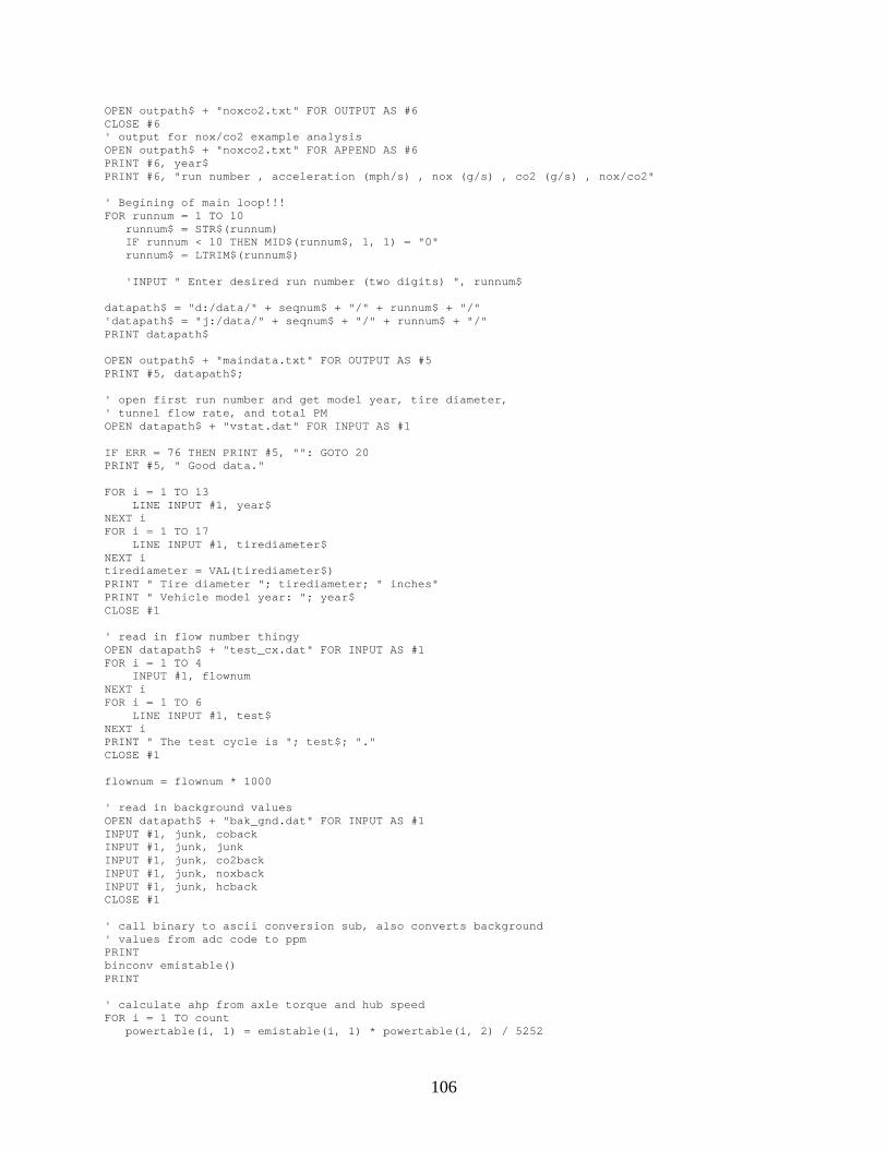
106

OPEN outpath$ + "noxco2.txt" FOR OUTPUT AS #6CLOSE #6' output for nox/co2 example analysisOPEN outpath$ + "noxco2.txt" FOR APPEND AS #6PRINT #6, year$PRINT #6, "run number , acceleration (mph/s) , nox (g/s) , co2 (g/s) , nox/co2"

' Begining of main loop!!!FOR runnum = 1 TO 10 runnum$ = STR$(runnum) IF runnum < 10 THEN MID$(runnum$, 1, 1) = "0" runnum$ = LTRIM$(runnum$)

'INPUT " Enter desired run number (two digits) ", runnum$

datapath$ = "d:/data/" + seqnum$ + "/" + runnum$ + "/"'datapath$ = "j:/data/" + seqnum$ + "/" + runnum$ + "/"PRINT datapath$

OPEN outpath$ + "maindata.txt" FOR OUTPUT AS #5PRINT #5, datapath$;

' open first run number and get model year, tire diameter,' tunnel flow rate, and total PMOPEN datapath$ + "vstat.dat" FOR INPUT AS #1

IF ERR = 76 THEN PRINT #5, "": GOTO 20PRINT #5, " Good data."

FOR i = 1 TO 13 LINE INPUT #1, year$NEXT iFOR i = 1 TO 17 LINE INPUT #1, tirediameter$NEXT itirediameter = VAL(tirediameter$)PRINT " Tire diameter "; tirediameter; " inches"PRINT " Vehicle model year: "; year$CLOSE #1

' read in flow number thingyOPEN datapath$ + "test_cx.dat" FOR INPUT AS #1FOR i = 1 TO 4 INPUT #1, flownumNEXT iFOR i = 1 TO 6 LINE INPUT #1, test$NEXT iPRINT " The test cycle is "; test$; "."CLOSE #1

flownum = flownum * 1000

' read in background valuesOPEN datapath$ + "bak_gnd.dat" FOR INPUT AS #1INPUT #1, junk, cobackINPUT #1, junk, junkINPUT #1, junk, co2backINPUT #1, junk, noxbackINPUT #1, junk, hcbackCLOSE #1

' call binary to ascii conversion sub, also converts background' values from adc code to ppmPRINTbinconv emistable()PRINT

' calculate ahp from axle torque and hub speedFOR i = 1 TO count powertable(i, 1) = emistable(i, 1) * powertable(i, 2) / 5252

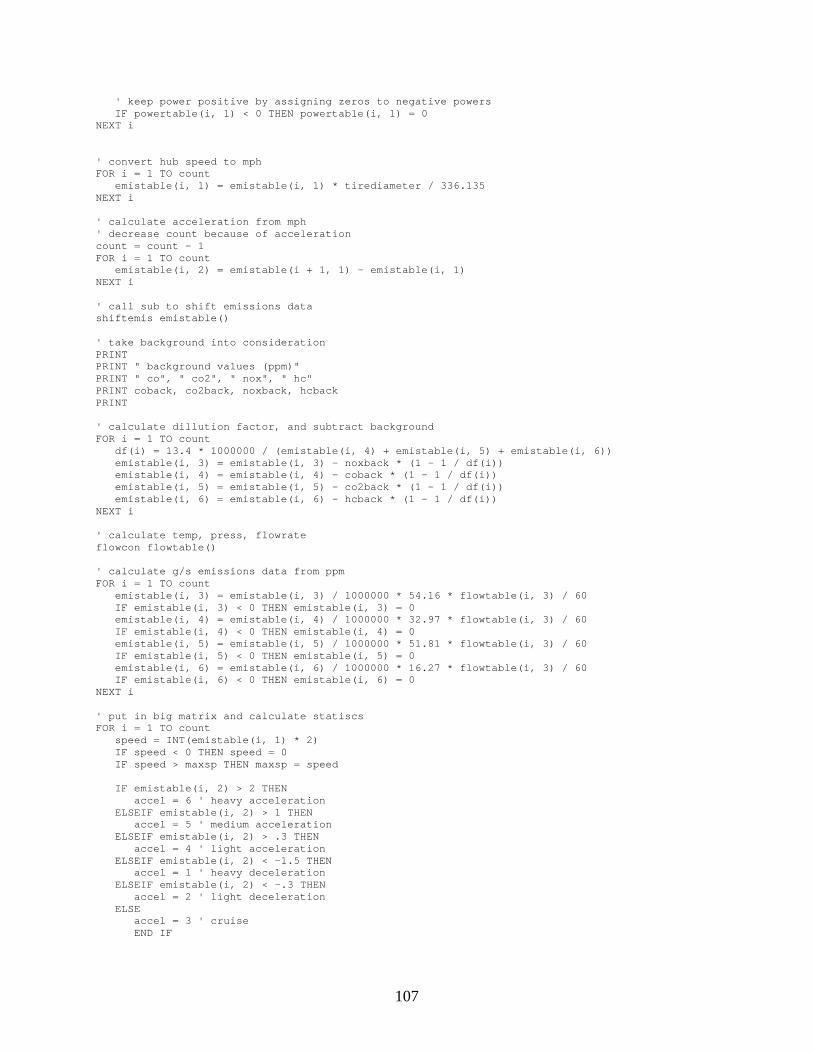
107

' keep power positive by assigning zeros to negative powers IF powertable(i, 1) < 0 THEN powertable(i, 1) = 0NEXT i

' convert hub speed to mphFOR i = 1 TO count emistable(i, 1) = emistable(i, 1) * tirediameter / 336.135NEXT i

' calculate acceleration from mph' decrease count because of accelerationcount = count - 1FOR i = 1 TO count emistable(i, 2) = emistable(i + 1, 1) - emistable(i, 1)NEXT i

' call sub to shift emissions datashiftemis emistable()

' take background into considerationPRINTPRINT " background values (ppm)"PRINT " co", " co2", " nox", " hc"PRINT coback, co2back, noxback, hcbackPRINT

' calculate dillution factor, and subtract backgroundFOR i = 1 TO count df(i) = 13.4 * 1000000 / (emistable(i, 4) + emistable(i, 5) + emistable(i, 6)) emistable(i, 3) = emistable(i, 3) - noxback * (1 - 1 / df(i)) emistable(i, 4) = emistable(i, 4) - coback * (1 - 1 / df(i)) emistable(i, 5) = emistable(i, 5) - co2back * (1 - 1 / df(i)) emistable(i, 6) = emistable(i, 6) - hcback * (1 - 1 / df(i))NEXT i

' calculate temp, press, flowrateflowcon flowtable()

' calculate g/s emissions data from ppmFOR i = 1 TO count emistable(i, 3) = emistable(i, 3) / 1000000 * 54.16 * flowtable(i, 3) / 60 IF emistable(i, 3) < 0 THEN emistable(i, 3) = 0 emistable(i, 4) = emistable(i, 4) / 1000000 * 32.97 * flowtable(i, 3) / 60 IF emistable(i, 4) < 0 THEN emistable(i, 4) = 0 emistable(i, 5) = emistable(i, 5) / 1000000 * 51.81 * flowtable(i, 3) / 60 IF emistable(i, 5) < 0 THEN emistable(i, 5) = 0 emistable(i, 6) = emistable(i, 6) / 1000000 * 16.27 * flowtable(i, 3) / 60 IF emistable(i, 6) < 0 THEN emistable(i, 6) = 0NEXT i

' put in big matrix and calculate statiscsFOR i = 1 TO count speed = INT(emistable(i, 1) * 2) IF speed < 0 THEN speed = 0 IF speed > maxsp THEN maxsp = speed

IF emistable(i, 2) > 2 THEN accel = 6 ' heavy acceleration ELSEIF emistable(i, 2) > 1 THEN accel = 5 ' medium acceleration ELSEIF emistable(i, 2) > .3 THEN accel = 4 ' light acceleration ELSEIF emistable(i, 2) < -1.5 THEN accel = 1 ' heavy deceleration ELSEIF emistable(i, 2) < -.3 THEN accel = 2 ' light deceleration ELSE accel = 3 ' cruise END IF

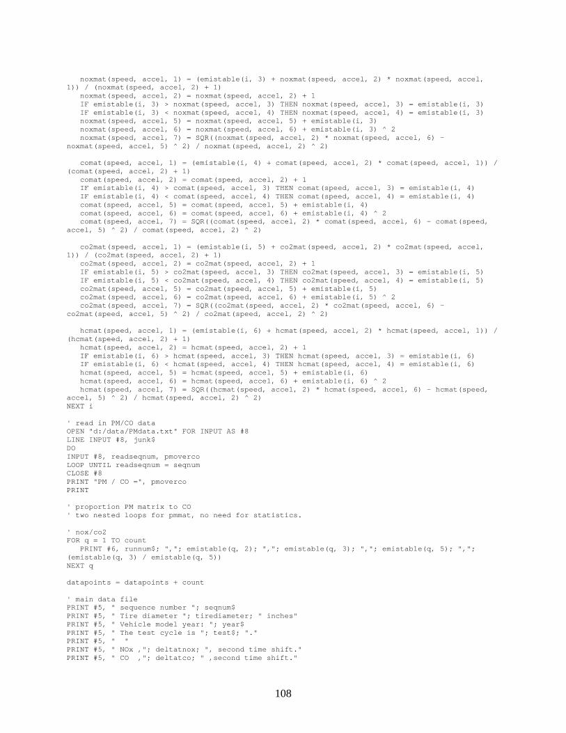
108

noxmat(speed, accel, 1) = (emistable(i, 3) + noxmat(speed, accel, 2) * noxmat(speed, accel,1)) / (noxmat(speed, accel, 2) + 1) noxmat(speed, accel, 2) = noxmat(speed, accel, 2) + 1 IF emistable(i, 3) > noxmat(speed, accel, 3) THEN noxmat(speed, accel, 3) = emistable(i, 3) IF emistable(i, 3) < noxmat(speed, accel, 4) THEN noxmat(speed, accel, 4) = emistable(i, 3) noxmat(speed, accel, 5) = noxmat(speed, accel, 5) + emistable(i, 3) noxmat(speed, accel, 6) = noxmat(speed, accel, 6) + emistable(i, 3) ^ 2 noxmat(speed, accel, 7) = SQR((noxmat(speed, accel, 2) * noxmat(speed, accel, 6) -noxmat(speed, accel, 5) ^ 2) / noxmat(speed, accel, 2) ^ 2)

comat(speed, accel, 1) = (emistable(i, 4) + comat(speed, accel, 2) * comat(speed, accel, 1)) /(comat(speed, accel, 2) + 1) comat(speed, accel, 2) = comat(speed, accel, 2) + 1 IF emistable(i, 4) > comat(speed, accel, 3) THEN comat(speed, accel, 3) = emistable(i, 4) IF emistable(i, 4) < comat(speed, accel, 4) THEN comat(speed, accel, 4) = emistable(i, 4) comat(speed, accel, 5) = comat(speed, accel, 5) + emistable(i, 4) comat(speed, accel, 6) = comat(speed, accel, 6) + emistable(i, 4) ^ 2 comat(speed, accel, 7) = SQR((comat(speed, accel, 2) * comat(speed, accel, 6) - comat(speed,accel, 5) ^ 2) / comat(speed, accel, 2) ^ 2)

co2mat(speed, accel, 1) = (emistable(i, 5) + co2mat(speed, accel, 2) * co2mat(speed, accel,1)) / (co2mat(speed, accel, 2) + 1) co2mat(speed, accel, 2) = co2mat(speed, accel, 2) + 1 IF emistable(i, 5) > co2mat(speed, accel, 3) THEN co2mat(speed, accel, 3) = emistable(i, 5) IF emistable(i, 5) < co2mat(speed, accel, 4) THEN co2mat(speed, accel, 4) = emistable(i, 5) co2mat(speed, accel, 5) = co2mat(speed, accel, 5) + emistable(i, 5) co2mat(speed, accel, 6) = co2mat(speed, accel, 6) + emistable(i, 5) ^ 2 co2mat(speed, accel, 7) = SQR((co2mat(speed, accel, 2) * co2mat(speed, accel, 6) -co2mat(speed, accel, 5) ^ 2) / co2mat(speed, accel, 2) ^ 2)

hcmat(speed, accel, 1) = (emistable(i, 6) + hcmat(speed, accel, 2) * hcmat(speed, accel, 1)) /(hcmat(speed, accel, 2) + 1) hcmat(speed, accel, 2) = hcmat(speed, accel, 2) + 1 IF emistable(i, 6) > hcmat(speed, accel, 3) THEN hcmat(speed, accel, 3) = emistable(i, 6) IF emistable(i, 6) < hcmat(speed, accel, 4) THEN hcmat(speed, accel, 4) = emistable(i, 6) hcmat(speed, accel, 5) = hcmat(speed, accel, 5) + emistable(i, 6) hcmat(speed, accel, 6) = hcmat(speed, accel, 6) + emistable(i, 6) ^ 2 hcmat(speed, accel, 7) = SQR((hcmat(speed, accel, 2) * hcmat(speed, accel, 6) - hcmat(speed,accel, 5) ^ 2) / hcmat(speed, accel, 2) ^ 2)NEXT i

' read in PM/CO dataOPEN "d:/data/PMdata.txt" FOR INPUT AS #8LINE INPUT #8, junk$DOINPUT #8, readseqnum, pmovercoLOOP UNTIL readseqnum = seqnumCLOSE #8PRINT "PM / CO =", pmovercoPRINT

' proportion PM matrix to CO' two nested loops for pmmat, no need for statistics.

' nox/co2FOR q = 1 TO count PRINT #6, runnum$; ","; emistable(q, 2); ","; emistable(q, 3); ","; emistable(q, 5); ",";(emistable(q, 3) / emistable(q, 5))NEXT q

datapoints = datapoints + count

' main data filePRINT #5, " sequence number "; seqnum$PRINT #5, " Tire diameter "; tirediameter; " inches"PRINT #5, " Vehicle model year: "; year$PRINT #5, " The test cycle is "; test$; "."PRINT #5, " "PRINT #5, " NOx ,"; deltatnox; ", second time shift."PRINT #5, " CO ,"; deltatco; " ,second time shift."

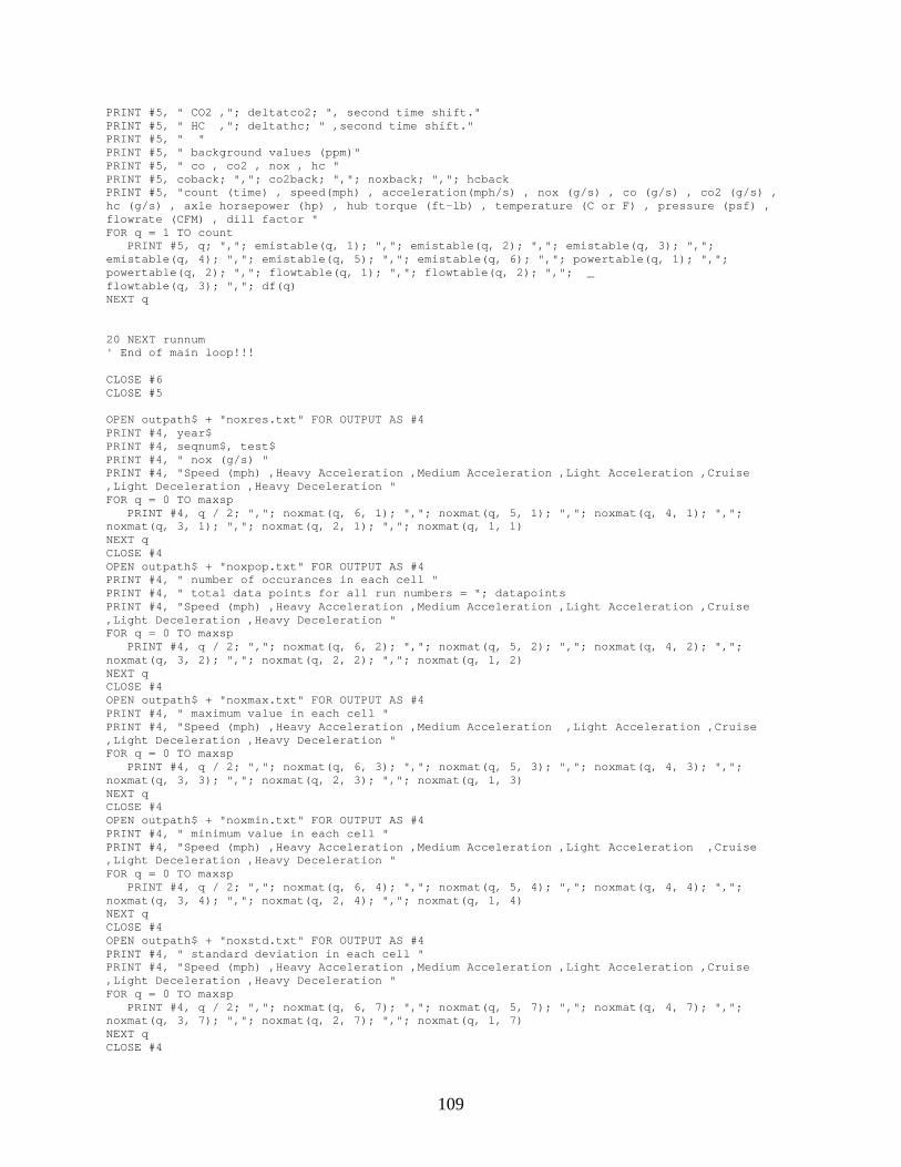
109

PRINT #5, " CO2 ,"; deltatco2; ", second time shift."PRINT #5, " HC ,"; deltathc; " ,second time shift."PRINT #5, " "PRINT #5, " background values (ppm)"PRINT #5, " co , co2 , nox , hc "PRINT #5, coback; ","; co2back; ","; noxback; ","; hcbackPRINT #5, "count (time) , speed(mph) , acceleration(mph/s) , nox (g/s) , co (g/s) , co2 (g/s) ,hc (g/s) , axle horsepower (hp) , hub torque (ft-lb) , temperature (C or F) , pressure (psf) ,flowrate (CFM) , dill factor "FOR q = 1 TO count PRINT #5, q; ","; emistable(q, 1); ","; emistable(q, 2); ","; emistable(q, 3); ",";emistable(q, 4); ","; emistable(q, 5); ","; emistable(q, 6); ","; powertable(q, 1); ",";powertable(q, 2); ","; flowtable(q, 1); ","; flowtable(q, 2); ","; _flowtable(q, 3); ","; df(q)NEXT q

20 NEXT runnum' End of main loop!!!

CLOSE #6CLOSE #5

OPEN outpath$ + "noxres.txt" FOR OUTPUT AS #4PRINT #4, year$PRINT #4, seqnum$, test$PRINT #4, " nox (g/s) "PRINT #4, "Speed (mph) ,Heavy Acceleration ,Medium Acceleration ,Light Acceleration ,Cruise,Light Deceleration ,Heavy Deceleration "FOR q = 0 TO maxsp PRINT #4, q / 2; ","; noxmat(q, 6, 1); ","; noxmat(q, 5, 1); ","; noxmat(q, 4, 1); ",";noxmat(q, 3, 1); ","; noxmat(q, 2, 1); ","; noxmat(q, 1, 1)NEXT qCLOSE #4OPEN outpath$ + "noxpop.txt" FOR OUTPUT AS #4PRINT #4, " number of occurances in each cell "PRINT #4, " total data points for all run numbers = "; datapointsPRINT #4, "Speed (mph) ,Heavy Acceleration ,Medium Acceleration ,Light Acceleration ,Cruise,Light Deceleration ,Heavy Deceleration "FOR q = 0 TO maxsp PRINT #4, q / 2; ","; noxmat(q, 6, 2); ","; noxmat(q, 5, 2); ","; noxmat(q, 4, 2); ",";noxmat(q, 3, 2); ","; noxmat(q, 2, 2); ","; noxmat(q, 1, 2)NEXT qCLOSE #4OPEN outpath$ + "noxmax.txt" FOR OUTPUT AS #4PRINT #4, " maximum value in each cell "PRINT #4, "Speed (mph) ,Heavy Acceleration ,Medium Acceleration ,Light Acceleration ,Cruise,Light Deceleration ,Heavy Deceleration "FOR q = 0 TO maxsp PRINT #4, q / 2; ","; noxmat(q, 6, 3); ","; noxmat(q, 5, 3); ","; noxmat(q, 4, 3); ",";noxmat(q, 3, 3); ","; noxmat(q, 2, 3); ","; noxmat(q, 1, 3)NEXT qCLOSE #4OPEN outpath$ + "noxmin.txt" FOR OUTPUT AS #4PRINT #4, " minimum value in each cell "PRINT #4, "Speed (mph) ,Heavy Acceleration ,Medium Acceleration ,Light Acceleration ,Cruise,Light Deceleration ,Heavy Deceleration "FOR q = 0 TO maxsp PRINT #4, q / 2; ","; noxmat(q, 6, 4); ","; noxmat(q, 5, 4); ","; noxmat(q, 4, 4); ",";noxmat(q, 3, 4); ","; noxmat(q, 2, 4); ","; noxmat(q, 1, 4)NEXT qCLOSE #4OPEN outpath$ + "noxstd.txt" FOR OUTPUT AS #4PRINT #4, " standard deviation in each cell "PRINT #4, "Speed (mph) ,Heavy Acceleration ,Medium Acceleration ,Light Acceleration ,Cruise,Light Deceleration ,Heavy Deceleration "FOR q = 0 TO maxsp PRINT #4, q / 2; ","; noxmat(q, 6, 7); ","; noxmat(q, 5, 7); ","; noxmat(q, 4, 7); ",";noxmat(q, 3, 7); ","; noxmat(q, 2, 7); ","; noxmat(q, 1, 7)NEXT qCLOSE #4

110

OPEN outpath$ + "cores.txt" FOR OUTPUT AS #4PRINT #4, year$PRINT #4, seqnum$, test$PRINT #4, " co (g/s) "PRINT #4, "Speed (mph) ,Heavy Acceleration ,Medium Acceleration ,Light Acceleration ,Cruise,Light Deceleration ,Heavy Deceleration "FOR q = 0 TO maxsp PRINT #4, q / 2; ","; comat(q, 6, 1); ","; comat(q, 5, 1); ","; comat(q, 4, 1); ","; comat(q,3, 1); ","; comat(q, 2, 1); ","; comat(q, 1, 1)NEXT qCLOSE #4OPEN outpath$ + "copop.txt" FOR OUTPUT AS #4PRINT #4, " number of occurances in each cell "PRINT #4, " total data points for all run numbers = "; datapointsPRINT #4, "Speed (mph) ,Heavy Acceleration ,Medium Acceleration ,Light Acceleration ,Cruise,Light Deceleration ,Heavy Deceleration "FOR q = 0 TO maxsp PRINT #4, q / 2; ","; comat(q, 6, 2); ","; comat(q, 5, 2); ","; comat(q, 4, 2); ","; comat(q,3, 2); ","; comat(q, 2, 2); ","; comat(q, 1, 2)NEXT qCLOSE #4OPEN outpath$ + "comax.txt" FOR OUTPUT AS #4PRINT #4, " maximum value in each cell "PRINT #4, "Speed (mph) ,Heavy Acceleration ,Medium Acceleration ,Light Acceleration ,Cruise,Light Deceleration ,Heavy Deceleration "FOR q = 0 TO maxsp PRINT #4, q / 2; ","; comat(q, 6, 3); ","; comat(q, 5, 3); ","; comat(q, 4, 3); ","; comat(q,3, 3); ","; comat(q, 2, 3); ","; comat(q, 1, 3)NEXT qCLOSE #4OPEN outpath$ + "comin.txt" FOR OUTPUT AS #4PRINT #4, " minimum value in each cell "PRINT #4, "Speed (mph) ,Heavy Acceleration ,Medium Acceleration ,Light Acceleration ,Cruise,Light Deceleration ,Heavy Deceleration "FOR q = 0 TO maxsp PRINT #4, q / 2; ","; comat(q, 6, 4); ","; comat(q, 5, 4); ","; comat(q, 4, 4); ","; comat(q,3, 4); ","; comat(q, 2, 4); ","; comat(q, 1, 4)NEXT qCLOSE #4OPEN outpath$ + "costd.txt" FOR OUTPUT AS #4PRINT #4, " standard deviation in each cell "PRINT #4, "Speed (mph) ,Heavy Acceleration ,Medium Acceleration ,Light Acceleration ,Cruise,Light Deceleration ,Heavy Deceleration "FOR q = 0 TO maxsp PRINT #4, q / 2; ","; comat(q, 6, 7); ","; comat(q, 5, 7); ","; comat(q, 4, 7); ","; comat(q,3, 7); ","; comat(q, 2, 7); ","; comat(q, 1, 7)NEXT qCLOSE #4

OPEN outpath$ + "hcres.txt" FOR OUTPUT AS #4PRINT #4, year$PRINT #4, seqnum$, test$PRINT #4, " hc (g/s) "PRINT #4, "Speed (mph) ,Heavy Acceleration ,Medium Acceleration ,Light Acceleration ,Cruise,Light Deceleration ,Heavy Deceleration "FOR q = 0 TO maxsp PRINT #4, q / 2; ","; hcmat(q, 6, 1); ","; hcmat(q, 5, 1); ","; hcmat(q, 4, 1); ","; hcmat(q,3, 1); ","; hcmat(q, 2, 1); ","; hcmat(q, 1, 1)NEXT qCLOSE #4OPEN outpath$ + "hcpop.txt" FOR OUTPUT AS #4PRINT #4, " number of occurances in each cell "PRINT #4, " total data points for all run numbers = "; datapointsPRINT #4, "Speed (mph) ,Heavy Acceleration ,Medium Acceleration ,Light Acceleration ,Cruise,Light Deceleration ,Heavy Deceleration "FOR q = 0 TO maxsp PRINT #4, q / 2; ","; hcmat(q, 6, 2); ","; hcmat(q, 5, 2); ","; hcmat(q, 4, 2); ","; hcmat(q,3, 2); ","; hcmat(q, 2, 2); ","; hcmat(q, 1, 2)

111

NEXT qCLOSE #4OPEN outpath$ + "hcmax.txt" FOR OUTPUT AS #4PRINT #4, " maximum value in each cell "PRINT #4, "Speed (mph) ,Heavy Acceleration ,Medium Acceleration ,Light Acceleration ,Cruise,Light Deceleration ,Heavy Deceleration "FOR q = 0 TO maxsp PRINT #4, q / 2; ","; hcmat(q, 6, 3); ","; hcmat(q, 5, 3); ","; hcmat(q, 4, 3); ","; hcmat(q,3, 3); ","; hcmat(q, 2, 3); ","; hcmat(q, 1, 3)NEXT qCLOSE #4OPEN outpath$ + "hcmin.txt" FOR OUTPUT AS #4PRINT #4, " minimum value in each cell "PRINT #4, "Speed (mph) ,Heavy Acceleration ,Medium Acceleration ,Light Acceleration ,Cruise,Light Deceleration ,Heavy Deceleration "FOR q = 0 TO maxsp PRINT #4, q / 2; ","; hcmat(q, 6, 4); ","; hcmat(q, 5, 4); ","; hcmat(q, 4, 4); ","; hcmat(q,3, 4); ","; hcmat(q, 2, 4); ","; hcmat(q, 1, 4)NEXT qCLOSE #4OPEN outpath$ + "hcstd.txt" FOR OUTPUT AS #4PRINT #4, " standard deviation in each cell "PRINT #4, "Speed (mph) ,Heavy Acceleration ,Medium Acceleration ,Light Acceleration ,Cruise,Light Deceleration ,Heavy Deceleration "FOR q = 0 TO maxsp PRINT #4, q / 2; ","; hcmat(q, 6, 7); ","; hcmat(q, 5, 7); ","; hcmat(q, 4, 7); ","; hcmat(q,3, 7); ","; hcmat(q, 2, 7); ","; hcmat(q, 1, 7)NEXT qCLOSE #4

OPEN outpath$ + "co2res.txt" FOR OUTPUT AS #4PRINT #4, year$PRINT #4, seqnum$, test$PRINT #4, " co2 (g/s) "PRINT #4, "Speed (mph) ,Heavy Acceleration ,Medium Acceleration ,Light Acceleration ,Cruise,Light Deceleration ,Heavy Deceleration "FOR q = 0 TO maxsp PRINT #4, q / 2; ","; co2mat(q, 6, 1); ","; co2mat(q, 5, 1); ","; co2mat(q, 4, 1); ",";co2mat(q, 3, 1); ","; co2mat(q, 2, 1); ","; co2mat(q, 1, 1)NEXT qCLOSE #4OPEN outpath$ + "co2pop.txt" FOR OUTPUT AS #4PRINT #4, " number of occurances in each cell "PRINT #4, " total data points for all run numbers = "; datapointsPRINT #4, "Speed (mph) ,Heavy Acceleration ,Medium Acceleration ,Light Acceleration ,Cruise,Light Deceleration ,Heavy Deceleration "FOR q = 0 TO maxsp PRINT #4, q / 2; ","; co2mat(q, 6, 2); ","; co2mat(q, 5, 2); ","; co2mat(q, 4, 2); ",";co2mat(q, 3, 2); ","; co2mat(q, 2, 2); ","; co2mat(q, 1, 2)NEXT qCLOSE #4OPEN outpath$ + "co2max.txt" FOR OUTPUT AS #4PRINT #4, " maximum value in each cell "PRINT #4, "Speed (mph) ,Heavy Acceleration ,Medium Acceleration ,Light Acceleration ,Cruise,Light Deceleration ,Heavy Deceleration "FOR q = 0 TO maxsp PRINT #4, q / 2; ","; co2mat(q, 6, 3); ","; co2mat(q, 5, 3); ","; co2mat(q, 4, 3); ",";co2mat(q, 3, 3); ","; co2mat(q, 2, 3); ","; co2mat(q, 1, 3)NEXT qCLOSE #4OPEN outpath$ + "co2min.txt" FOR OUTPUT AS #4PRINT #4, " minimum value in each cell "PRINT #4, "Speed (mph) ,Heavy Acceleration ,Medium Acceleration ,Light Acceleration ,Cruise,Light Deceleration ,Heavy Deceleration "FOR q = 0 TO maxsp PRINT #4, q / 2; ","; co2mat(q, 6, 4); ","; co2mat(q, 5, 4); ","; co2mat(q, 4, 4); ",";co2mat(q, 3, 4); ","; co2mat(q, 2, 4); ","; co2mat(q, 1, 4)NEXT qCLOSE #4OPEN outpath$ + "co2std.txt" FOR OUTPUT AS #4

112

PRINT #4, " standard deviation in each cell "PRINT #4, "Speed (mph) ,Heavy Acceleration ,Medium Acceleration ,Light Acceleration ,Cruise,Light Deceleration ,Heavy Deceleration "FOR q = 0 TO maxsp PRINT #4, q / 2; ","; co2mat(q, 6, 7); ","; co2mat(q, 5, 7); ","; co2mat(q, 4, 7); ",";co2mat(q, 3, 7); ","; co2mat(q, 2, 7); ","; co2mat(q, 1, 7)NEXT qCLOSE #4

' read next sequence number

PRINTPRINT " Number of data points available for use= "; datapointsPRINT

PRINT " ** Hit the any key. ** "DOLOOP WHILE INKEY$ = ""

LOOP'****************************************************************

' TheEND

SUB binconv (A())

'****************************************************************' Display curve in engineering unit'' CalData and CurveData Passed in'' modified for use in the los alamos program... by justin'****************************************************************DIM bytelocation AS LONGDIM Loco AS LONGDIM adccode AS INTEGERDIM RealValue AS SINGLEDIM j AS INTEGERDIM i AS INTEGERDIM k AS INTEGER

DIM RealValueSum AS DOUBLEDIM AscFileName AS STRINGDIM CO(1 TO 4)DIM CO2(1 TO 4)DIM HC(1 TO 4)DIM nox(1 TO 4)DIM TQ1(1 TO 2)DIM TQ2(1 TO 2)DIM HS(1 TO 2)

PRINT " Reading binary file, please wait..."

IF seqnum >= 633 THEN totchan = 64ELSE totchan = 32END IF

'' open a file for store ASCII data''datapath$ = "c:\data\1045\01\"'OPEN datapath$ + "emisdata.asc" FOR OUTPUT AS #11

113

'read calibration dataOPEN datapath$ + "lco.cal" FOR INPUT AS #12LINE INPUT #12, junk$LINE INPUT #12, junk$FOR i = 1 TO 4 INPUT #12, CO(i)NEXT iCLOSE #12

OPEN datapath$ + "co2.cal" FOR INPUT AS #12LINE INPUT #12, junk$LINE INPUT #12, junk$FOR i = 1 TO 4 INPUT #12, CO2(i)NEXT iCLOSE #12

OPEN datapath$ + "hc.cal" FOR INPUT AS #12LINE INPUT #12, junk$LINE INPUT #12, junk$FOR i = 1 TO 2 INPUT #12, HC(i)NEXT iCLOSE #12

OPEN datapath$ + "nox.cal" FOR INPUT AS #12LINE INPUT #12, junk$LINE INPUT #12, junk$FOR i = 1 TO 4 INPUT #12, nox(i)NEXT iCLOSE #12

OPEN datapath$ + "hs1.cal" FOR INPUT AS #12LINE INPUT #12, junk$LINE INPUT #12, junk$FOR i = 1 TO 2 INPUT #12, HS(i)NEXT iCLOSE #12

OPEN datapath$ + "tq1.cal" FOR INPUT AS #12LINE INPUT #12, junk$LINE INPUT #12, junk$FOR i = 1 TO 2 INPUT #12, TQ1(i)NEXT iCLOSE #12

OPEN datapath$ + "tq2.cal" FOR INPUT AS #12LINE INPUT #12, junk$LINE INPUT #12, junk$FOR i = 1 TO 2 INPUT #12, TQ2(i)NEXT iCLOSE #12

' convert background adc code to ppmhcback = HC(1) + HC(2) * hcbackcoback = CO(1) + CO(2) * coback + CO(3) * coback ^ 2 + CO(4) * coback ^ 3co2back = CO2(1) + CO2(2) * co2back + CO2(3) * co2back ^ 2 + CO2(4) * co2back ^ 3noxback = nox(1) + nox(2) * noxback + nox(3) * noxback ^ 2 + nox(4) * noxback ^ 3

OPEN datapath$ + "cyc_bin.dat" FOR BINARY AS #1

numofscan = LOF(1) / totchan / 2

'' find the first data in the data file

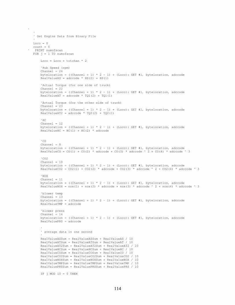
114

' ' ' Get Engine Data from Binary File ' Loco = 0 count = 0' PRINT numofscan FOR j = 1 TO numofscan

Loco = Loco + totchan * 2

'Hub Speed (rpm) Channel = 24 bytelocation = ((Channel + 1) * 2 - 1) + (Loco): GET #1, bytelocation, adccode RealValueAS = adccode * HS(2) + HS(1)

'Actual Torque (for one side of truck) Channel = 22 bytelocation = ((Channel + 1) * 2 - 1) + (Loco): GET #1, bytelocation, adccode RealValueAT = adccode * TQ1(2) + TQ1(1)

'Actual Torque (for the other side of truck) Channel = 23 bytelocation = ((Channel + 1) * 2 - 1) + (Loco): GET #1, bytelocation, adccode RealValueAT2 = adccode * TQ2(2) + TQ2(1)

'HC Channel = 12 bytelocation = ((Channel + 1) * 2 - 1) + (Loco): GET #1, bytelocation, adccode RealValueHC = HC(1) + HC(2) * adccode

'CO Channel = 8 bytelocation = ((Channel + 1) * 2 - 1) + (Loco): GET #1, bytelocation, adccode RealValueCO = CO(1) + CO(2) * adccode + CO(3) * adccode ^ 2 + CO(4) * adccode ^ 3

'CO2 Channel = 10 bytelocation = ((Channel + 1) * 2 - 1) + (Loco): GET #1, bytelocation, adccode RealValueCO2 = CO2(1) + CO2(2) * adccode + CO2(3) * adccode ^ 2 + CO2(4) * adccode ^ 3

'NOX Channel = 11 bytelocation = ((Channel + 1) * 2 - 1) + (Loco): GET #1, bytelocation, adccode RealValueNOX = nox(1) + nox(2) * adccode + nox(3) * adccode ^ 2 + nox(4) * adccode ^ 3

'blower temp Channel = 13 bytelocation = ((Channel + 1) * 2 - 1) + (Loco): GET #1, bytelocation, adccode RealValueTMP = adccode

'blower press Channel = 14 bytelocation = ((Channel + 1) * 2 - 1) + (Loco): GET #1, bytelocation, adccode RealValuePRS = adccode

' ' average data in one second ' RealValueASSum = RealValueASSum + RealValueAS / 10 RealValueATSum = RealValueATSum + RealValueAT / 10 RealValueAT2Sum = RealValueAT2Sum + RealValueAT2 / 10 RealValueHCSum = RealValueHCSum + RealValueHC / 10 RealValueCOSum = RealValueCOSum + RealValueCO / 10 RealValueCO2Sum = RealValueCO2Sum + RealValueCO2 / 10 RealValueNOXSum = RealValueNOXSum + RealValueNOX / 10 RealValueTMPSum = RealValueTMPSum + RealValueTMP / 10 RealValuePRSSum = RealValuePRSSum + RealValuePRS / 10

IF j MOD 10 = 0 THEN

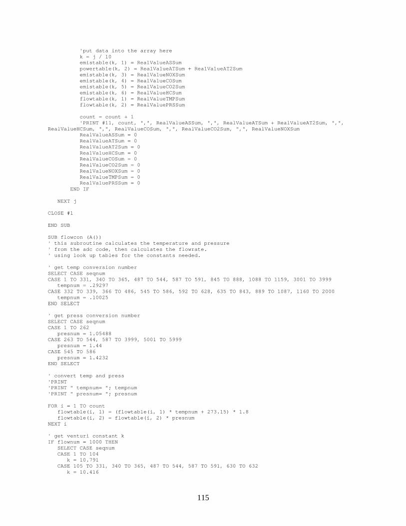
115

'put data into the array here k = j / 10 emistable(k, 1) = RealValueASSum powertable(k, 2) = RealValueATSum + RealValueAT2Sum emistable(k, 3) = RealValueNOXSum emistable(k, 4) = RealValueCOSum emistable(k, 5) = RealValueCO2Sum emistable(k, 6) = RealValueHCSum flowtable(k, 1) = RealValueTMPSum flowtable(k, 2) = RealValuePRSSum

count = count + 1 'PRINT #11, count, ",", RealValueASSum, ",", RealValueATSum + RealValueAT2Sum, ",",RealValueHCSum, ",", RealValueCOSum, ",", RealValueCO2Sum, ",", RealValueNOXSum RealValueASSum = 0 RealValueATSum = 0 RealValueAT2Sum = 0 RealValueHCSum = 0 RealValueCOSum = 0 RealValueCO2Sum = 0 RealValueNOXSum = 0 RealValueTMPSum = 0 RealValuePRSSum = 0 END IF

NEXT j

CLOSE #1

END SUB

SUB flowcon (A())' this subroutine calculates the temperature and pressure' from the adc code, then calculates the flowrate.' using look up tables for the constants needed.

' get temp conversion numberSELECT CASE seqnumCASE 1 TO 331, 340 TO 365, 487 TO 544, 587 TO 591, 845 TO 888, 1088 TO 1159, 3001 TO 3999 tempnum = .29297CASE 332 TO 339, 366 TO 486, 545 TO 586, 592 TO 628, 635 TO 843, 889 TO 1087, 1160 TO 2000 tempnum = .10025END SELECT

' get press conversion numberSELECT CASE seqnumCASE 1 TO 262 presnum = 1.05488CASE 263 TO 544, 587 TO 3999, 5001 TO 5999 presnum = 1.44CASE 545 TO 586 presnum = 1.4232END SELECT

' convert temp and press'PRINT'PRINT " tempnum= "; tempnum'PRINT " presnum= "; presnum

FOR i = 1 TO count flowtable(i, 1) = (flowtable(i, 1) * tempnum + 273.15) * 1.8 flowtable(i, 2) = flowtable(i, 2) * presnumNEXT i

' get venturi constant kIF flownum = 1000 THEN SELECT CASE seqnum CASE 1 TO 104 k = 10.791 CASE 105 TO 331, 340 TO 365, 487 TO 544, 587 TO 591, 630 TO 632 k = 10.416

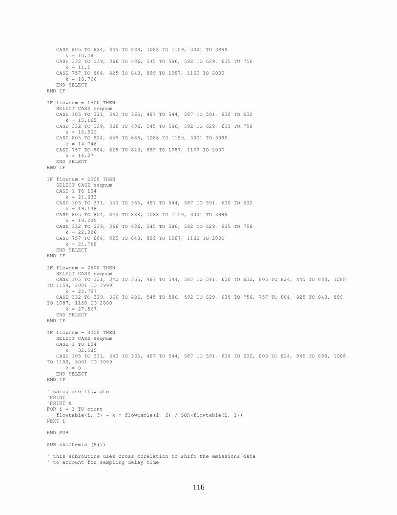
116

CASE 805 TO 824, 845 TO 888, 1088 TO 1159, 3001 TO 3999 k = 10.281 CASE 332 TO 339, 366 TO 486, 545 TO 586, 592 TO 629, 635 TO 756 k = 11.1 CASE 757 TO 804, 825 TO 843, 889 TO 1087, 1160 TO 2000 k = 10.766 END SELECTEND IF

IF flownum = 1500 THEN SELECT CASE seqnum CASE 105 TO 331, 340 TO 365, 487 TO 544, 587 TO 591, 630 TO 632 k = 15.165 CASE 332 TO 339, 366 TO 486, 545 TO 586, 592 TO 629, 635 TO 756 k = 16.502 CASE 805 TO 824, 845 TO 888, 1088 TO 1159, 3001 TO 3999 k = 14.746 CASE 757 TO 804, 825 TO 843, 889 TO 1087, 1160 TO 2000 k = 16.27 END SELECTEND IF

IF flownum = 2000 THEN SELECT CASE seqnum CASE 1 TO 104 k = 21.633 CASE 105 TO 331, 340 TO 365, 487 TO 544, 587 TO 591, 630 TO 632 k = 19.138 CASE 805 TO 824, 845 TO 888, 1088 TO 1159, 3001 TO 3999 k = 19.205 CASE 332 TO 339, 366 TO 486, 545 TO 586, 592 TO 629, 635 TO 756 k = 22.026 CASE 757 TO 804, 825 TO 843, 889 TO 1087, 1160 TO 2000 k = 21.768 END SELECTEND IF

IF flownum = 2500 THEN SELECT CASE seqnum CASE 105 TO 331, 340 TO 365, 487 TO 544, 587 TO 591, 630 TO 632, 805 TO 824, 845 TO 888, 1088TO 1159, 3001 TO 3999 k = 23.797 CASE 332 TO 339, 366 TO 486, 545 TO 586, 592 TO 629, 635 TO 756, 757 TO 804, 825 TO 843, 889TO 1087, 1160 TO 2000 k = 27.567 END SELECTEND IF

IF flownum = 3000 THEN SELECT CASE seqnum CASE 1 TO 104 k = 32.585 CASE 105 TO 331, 340 TO 365, 487 TO 544, 587 TO 591, 630 TO 632, 805 TO 824, 845 TO 888, 1088TO 1159, 3001 TO 3999 k = 0 END SELECTEND IF

' calculate flowrate'PRINT'PRINT kFOR i = 1 TO count flowtable(i, 3) = k * flowtable(i, 2) / SQR(flowtable(i, 1))NEXT i

END SUB

SUB shiftemis (A())

' this subroutine uses cross corelation to shift the emissions data' to account for sampling delay time

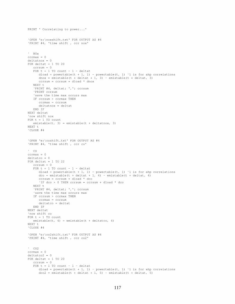
117

PRINT " Correlating to power..."

'OPEN "e:\noxshift.txt" FOR OUTPUT AS #4'PRINT #4, "time shift , ccr nox"

' NOxccrmax = 0deltatnox = 0FOR deltat = 1 TO 20 ccrsum = 0 FOR t = 1 TO count - 1 - deltat dload = powertable(t + 1, 1) - powertable(t, 1) '1 is for ahp correlations dnox = emistable(t + deltat + 1, 3) - emistable(t + deltat, 3) ccrsum = ccrsum + dload * dnox NEXT t 'PRINT #4, deltat; ","; ccrsum 'PRINT ccrsum 'save the time max occurs max IF ccrsum > ccrmax THEN ccrmax = ccrsum deltatnox = deltat END IFNEXT deltat'now shift noxFOR t = 1 TO count emistable(t, 3) = emistable(t + deltatnox, 3)NEXT t'CLOSE #4

'OPEN "e:\coshift.txt" FOR OUTPUT AS #4'PRINT #4, "time shift , ccr co"

' COccrmax = 0deltatco = 0FOR deltat = 1 TO 22 ccrsum = 0 FOR t = 1 TO count - 1 - deltat dload = powertable(t + 1, 1) - powertable(t, 1) '1 is for ahp correlations dco = emistable(t + deltat + 1, 4) - emistable(t + deltat, 4) ccrsum = ccrsum + dload * dco 'IF dco > 0 THEN ccrsum = ccrsum + dload * dco NEXT t 'PRINT #4, deltat; ","; ccrsum 'save the time max occurs max IF ccrsum > ccrmax THEN ccrmax = ccrsum deltatco = deltat END IFNEXT deltat'now shift coFOR t = 1 TO count emistable(t, 4) = emistable(t + deltatco, 4)NEXT t'CLOSE #4

'OPEN "e:\co2shift.txt" FOR OUTPUT AS #4'PRINT #4, "time shift , ccr co2"

' CO2ccrmax = 0deltatco2 = 0FOR deltat = 1 TO 20 ccrsum = 0 FOR t = 1 TO count - 1 - deltat dload = powertable(t + 1, 1) - powertable(t, 1) '1 is for ahp correlations dco2 = emistable(t + deltat + 1, 5) - emistable(t + deltat, 5)

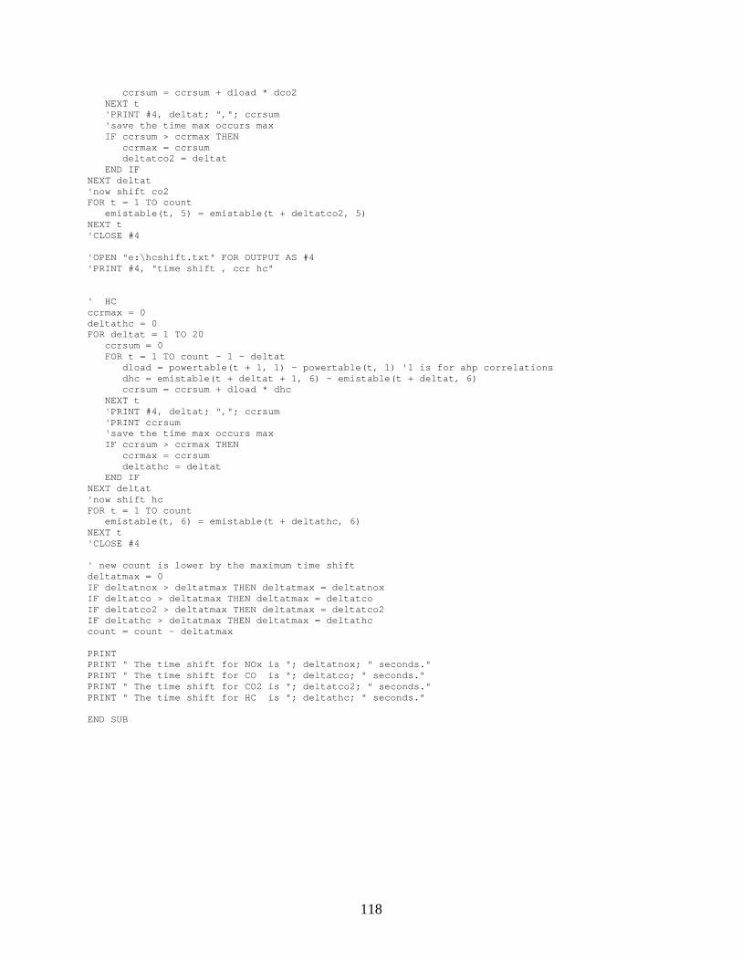
118

ccrsum = ccrsum + dload * dco2 NEXT t 'PRINT #4, deltat; ","; ccrsum 'save the time max occurs max IF ccrsum > ccrmax THEN ccrmax = ccrsum deltatco2 = deltat END IFNEXT deltat'now shift co2FOR t = 1 TO count emistable(t, 5) = emistable(t + deltatco2, 5)NEXT t'CLOSE #4

'OPEN "e:\hcshift.txt" FOR OUTPUT AS #4'PRINT #4, "time shift , ccr hc"

' HCccrmax = 0deltathc = 0FOR deltat = 1 TO 20 ccrsum = 0 FOR t = 1 TO count - 1 - deltat dload = powertable(t + 1, 1) - powertable(t, 1) '1 is for ahp correlations dhc = emistable(t + deltat + 1, 6) - emistable(t + deltat, 6) ccrsum = ccrsum + dload * dhc NEXT t 'PRINT #4, deltat; ","; ccrsum 'PRINT ccrsum 'save the time max occurs max IF ccrsum > ccrmax THEN ccrmax = ccrsum deltathc = deltat END IFNEXT deltat'now shift hcFOR t = 1 TO count emistable(t, 6) = emistable(t + deltathc, 6)NEXT t'CLOSE #4

' new count is lower by the maximum time shiftdeltatmax = 0IF deltatnox > deltatmax THEN deltatmax = deltatnoxIF deltatco > deltatmax THEN deltatmax = deltatcoIF deltatco2 > deltatmax THEN deltatmax = deltatco2IF deltathc > deltatmax THEN deltatmax = deltathccount = count - deltatmax

PRINTPRINT " The time shift for NOx is "; deltatnox; " seconds."PRINT " The time shift for CO is "; deltatco; " seconds."PRINT " The time shift for CO2 is "; deltatco2; " seconds."PRINT " The time shift for HC is "; deltathc; " seconds."

END SUB

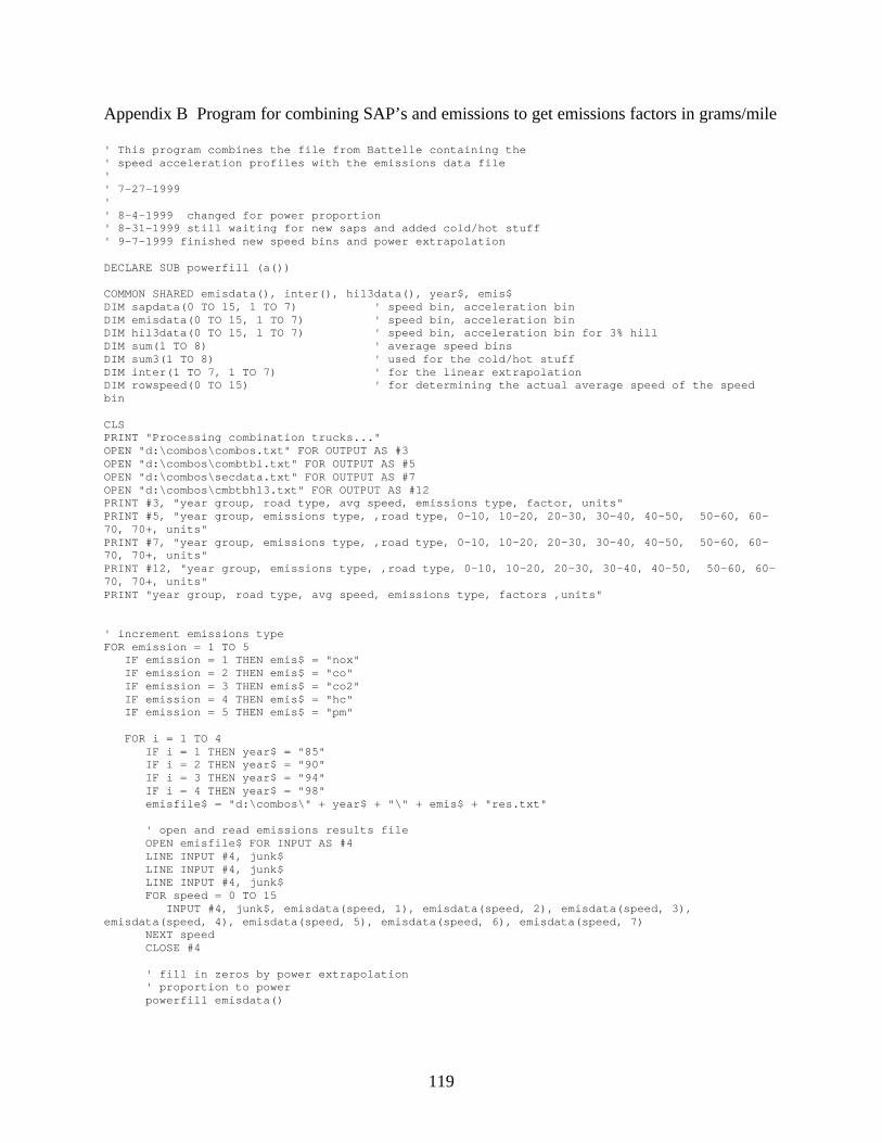
119

Appendix B Program for combining SAP’s and emissions to get emissions factors in grams/mile

' This program combines the file from Battelle containing the' speed acceleration profiles with the emissions data file'' 7-27-1999'' 8-4-1999 changed for power proportion' 8-31-1999 still waiting for new saps and added cold/hot stuff' 9-7-1999 finished new speed bins and power extrapolation

DECLARE SUB powerfill (a())

COMMON SHARED emisdata(), inter(), hil3data(), year$, emis$DIM sapdata(0 TO 15, 1 TO 7) ' speed bin, acceleration binDIM emisdata(0 TO 15, 1 TO 7) ' speed bin, acceleration binDIM hil3data(0 TO 15, 1 TO 7) ' speed bin, acceleration bin for 3% hillDIM sum(1 TO 8) ' average speed binsDIM sum3(1 TO 8) ' used for the cold/hot stuffDIM inter(1 TO 7, 1 TO 7) ' for the linear extrapolationDIM rowspeed(0 TO 15) ' for determining the actual average speed of the speedbin

CLSPRINT "Processing combination trucks..."OPEN "d:\combos\combos.txt" FOR OUTPUT AS #3OPEN "d:\combos\combtbl.txt" FOR OUTPUT AS #5OPEN "d:\combos\secdata.txt" FOR OUTPUT AS #7OPEN "d:\combos\cmbtbhl3.txt" FOR OUTPUT AS #12PRINT #3, "year group, road type, avg speed, emissions type, factor, units"PRINT #5, "year group, emissions type, ,road type, 0-10, 10-20, 20-30, 30-40, 40-50, 50-60, 60-70, 70+, units"PRINT #7, "year group, emissions type, ,road type, 0-10, 10-20, 20-30, 30-40, 40-50, 50-60, 60-70, 70+, units"PRINT #12, "year group, emissions type, ,road type, 0-10, 10-20, 20-30, 30-40, 40-50, 50-60, 60-70, 70+, units"PRINT "year group, road type, avg speed, emissions type, factors ,units"

' increment emissions typeFOR emission = 1 TO 5 IF emission = 1 THEN emis$ = "nox" IF emission = 2 THEN emis$ = "co" IF emission = 3 THEN emis$ = "co2" IF emission = 4 THEN emis$ = "hc" IF emission = 5 THEN emis$ = "pm"

FOR i = 1 TO 4 IF i = 1 THEN year$ = "85" IF i = 2 THEN year$ = "90" IF i = 3 THEN year$ = "94" IF i = 4 THEN year$ = "98" emisfile$ = "d:\combos\" + year$ + "\" + emis$ + "res.txt"

' open and read emissions results file OPEN emisfile$ FOR INPUT AS #4 LINE INPUT #4, junk$ LINE INPUT #4, junk$ LINE INPUT #4, junk$ FOR speed = 0 TO 15 INPUT #4, junk$, emisdata(speed, 1), emisdata(speed, 2), emisdata(speed, 3),emisdata(speed, 4), emisdata(speed, 5), emisdata(speed, 6), emisdata(speed, 7) NEXT speed CLOSE #4

' fill in zeros by power extrapolation ' proportion to power powerfill emisdata()

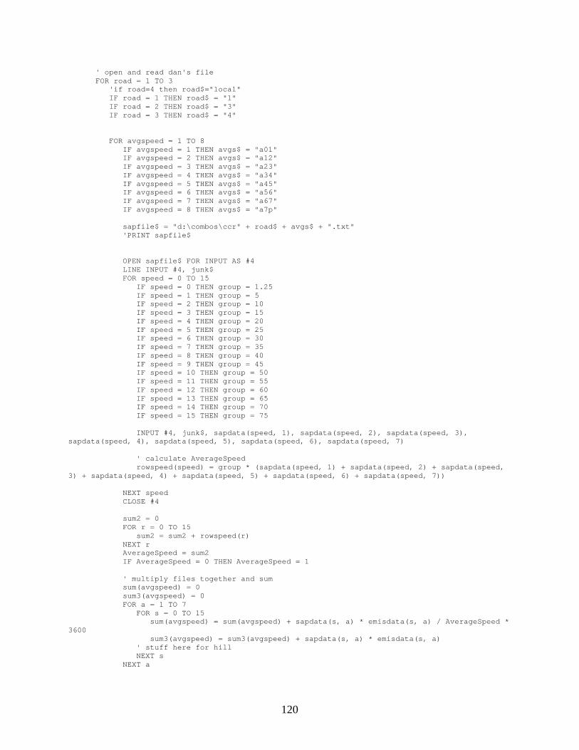
120

' open and read dan's file FOR road = 1 TO 3 'if road=4 then road$="local" IF road = 1 THEN road$ = "1" IF road = 2 THEN road$ = "3" IF road = 3 THEN road$ = "4"

FOR avgspeed = 1 TO 8 IF avgspeed = 1 THEN avgs$ = "a01" IF avgspeed = 2 THEN avgs$ = "a12" IF avgspeed = 3 THEN avgs$ = "a23" IF avgspeed = 4 THEN avgs$ = "a34" IF avgspeed = 5 THEN avgs$ = "a45" IF avgspeed = 6 THEN avgs$ = "a56" IF avgspeed = 7 THEN avgs$ = "a67" IF avgspeed = 8 THEN avgs$ = "a7p"

sapfile$ = "d:\combos\ccr" + road$ + avgs$ + ".txt" 'PRINT sapfile$

OPEN sapfile$ FOR INPUT AS #4 LINE INPUT #4, junk$ FOR speed = 0 TO 15 IF speed = 0 THEN group = 1.25 IF speed = 1 THEN group = 5 IF speed = 2 THEN group = 10 IF speed = 3 THEN group = 15 IF speed = 4 THEN group = 20 IF speed = 5 THEN group = 25 IF speed = 6 THEN group = 30 IF speed = 7 THEN group = 35 IF speed = 8 THEN group = 40 IF speed = 9 THEN group = 45 IF speed = 10 THEN group = 50 IF speed = 11 THEN group = 55 IF speed = 12 THEN group = 60 IF speed = 13 THEN group = 65 IF speed = 14 THEN group = 70 IF speed = 15 THEN group = 75

INPUT #4, junk$, sapdata(speed, 1), sapdata(speed, 2), sapdata(speed, 3),sapdata(speed, 4), sapdata(speed, 5), sapdata(speed, 6), sapdata(speed, 7)

' calculate AverageSpeed rowspeed(speed) = group * (sapdata(speed, 1) + sapdata(speed, 2) + sapdata(speed,3) + sapdata(speed, 4) + sapdata(speed, 5) + sapdata(speed, 6) + sapdata(speed, 7))

NEXT speed CLOSE #4

sum2 = 0 FOR r = 0 TO 15 sum2 = sum2 + rowspeed(r) NEXT r AverageSpeed = sum2 IF AverageSpeed = 0 THEN AverageSpeed = 1

' multiply files together and sum sum(avgspeed) = 0 sum3(avgspeed) = 0 FOR a = 1 TO 7 FOR s = 0 TO 15 sum(avgspeed) = sum(avgspeed) + sapdata(s, a) * emisdata(s, a) / AverageSpeed *3600 sum3(avgspeed) = sum3(avgspeed) + sapdata(s, a) * emisdata(s, a) ' stuff here for hill NEXT s NEXT a

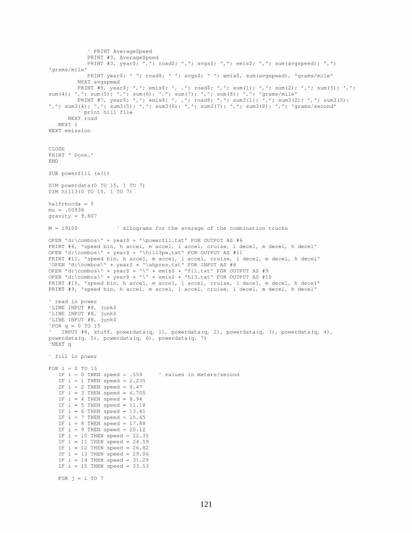
121

' PRINT AverageSpeed PRINT #3, AverageSpeed PRINT #3, year$; ","; road$; ","; avgs$; ","; emis$; ","; sum(avgspeed); ",";"grams/mile" PRINT year$; " "; road$; " "; avgs$; " "; emis$, sum(avgspeed), "grams/mile" NEXT avgspeed PRINT #5, year$; ","; emis$; ", ,"; road$; ","; sum(1); ","; sum(2); ","; sum(3); ",";sum(4); ","; sum(5); ","; sum(6); ","; sum(7); ","; sum(8); ","; "grams/mile" PRINT #7, year$; ","; emis$; ", ,"; road$; ","; sum3(1); ","; sum3(2); ","; sum3(3);","; sum3(4); ","; sum3(5); ","; sum3(6); ","; sum3(7); ","; sum3(8); ","; "grams/second" ' print hill file NEXT road NEXT iNEXT emission

CLOSEPRINT " Done."END

SUB powerfill (a())

DIM powerdata(0 TO 15, 1 TO 7)DIM hill3(0 TO 15, 1 TO 7)

halfrhocda = 5mu = .00938gravity = 9.807

M = 19100 ' kilograms for the average of the combination trucks

OPEN "d:\combos\" + year$ + "\powerfil.txt" FOR OUTPUT AS #6PRINT #6, "speed bin, h accel, m accel, l accel, cruise, l decel, m decel, h decel"OPEN "d:\combos\" + year$ + "\hill3pw.txt" FOR OUTPUT AS #11PRINT #11, "speed bin, h accel, m accel, l accel, cruise, l decel, m decel, h decel"'OPEN "d:\combos\" + year$ + "\ahpres.txt" FOR INPUT AS #8OPEN "d:\combos\" + year$ + "\" + emis$ + "fil.txt" FOR OUTPUT AS #9OPEN "d:\combos\" + year$ + "\" + emis$ + "hl3.txt" FOR OUTPUT AS #10PRINT #10, "speed bin, h accel, m accel, l accel, cruise, l decel, m decel, h decel"PRINT #9, "speed bin, h accel, m accel, l accel, cruise, l decel, m decel, h decel"

' read in power'LINE INPUT #8, junk$'LINE INPUT #8, junk$'LINE INPUT #8, junk$'FOR q = 0 TO 15' INPUT #8, stuff, powerdata(q, 1), powerdata(q, 2), powerdata(q, 3), powerdata(q, 4),powerdata(q, 5), powerdata(q, 6), powerdata(q, 7)'NEXT q

' fill in power

FOR i = 0 TO 15 IF i = 0 THEN speed = .559 ' values in meters/second IF i = 1 THEN speed = 2.235 IF i = 2 THEN speed = 4.47 IF i = 3 THEN speed = 6.705 IF i = 4 THEN speed = 8.94 IF i = 5 THEN speed = 11.18 IF i = 6 THEN speed = 13.41 IF i = 7 THEN speed = 15.65 IF i = 8 THEN speed = 17.88 IF i = 9 THEN speed = 20.12 IF i = 10 THEN speed = 22.35 IF i = 11 THEN speed = 24.59 IF i = 12 THEN speed = 26.82 IF i = 13 THEN speed = 29.06 IF i = 14 THEN speed = 31.29 IF i = 15 THEN speed = 33.53

FOR j = 1 TO 7

122

IF j = 1 THEN accel = .9 ' values in meters/second^2 IF j = 2 THEN accel = .66 IF j = 3 THEN accel = .29 IF j = 4 THEN accel = 0 IF j = 5 THEN accel = -.29 IF j = 6 THEN accel = -.66 IF j = 7 THEN accel = -.9 powerdata(i, j) = (halfrhocda * speed ^ 3 + M * accel * speed + mu * M * g * speed) / 745.7 hill3(i, j) = (halfrhocda * speed ^ 3 + M * accel * speed + mu * M * g * speed + M * g *speed * .03) / 745.7 NEXT j PRINT #6, speed; ","; powerdata(i, 1); ","; powerdata(i, 2); ","; powerdata(i, 3); ",";powerdata(i, 4); ","; powerdata(i, 5); ","; powerdata(i, 6); ","; powerdata(i, 7) PRINT #11, speed; ","; hill3(i, 1); ","; hill3(i, 2); ","; hill3(i, 3); ","; hill3(i, 4); ",";hill3(i, 5); ","; hill3(i, 6); ","; hill3(i, 7)NEXT iCLOSE #6CLOSE #11

' fit curves to power/emissions data

' fill interp with zeros FOR x = 1 TO 7 FOR y = 1 TO 7 inter(x, y) = 0! NEXT y NEXT x

' calculate sums

FOR accel = 1 TO 7 FOR speed = 0 TO 15

IF emisdata(speed, accel) <> 0 THEN inter(1, accel) = inter(1, accel) + emisdata(speed, accel) ' sum of y inter(2, accel) = inter(2, accel) + emisdata(speed, accel) * powerdata(speed,accel) 'sum of xy inter(5, accel) = inter(5, accel) + powerdata(speed, accel) ' sum of x inter(6, accel) = inter(6, accel) + powerdata(speed, accel) ^ 2 ' sum of xsquared inter(7, accel) = inter(7, accel) + 1 ' n END IF NEXT speed ' PRINT ' PRINT emis$, year$, inter(7, accel), inter(5, accel), inter(6, accel) ' PRINT inter(1, accel), inter(2, accel) NEXT accel

' calculate m and b FOR accel = 1 TO 7 inter(3, accel) = (inter(7, accel) * inter(2, accel) - inter(5, accel) * inter(1,accel)) / (inter(7, accel) * inter(6, accel) - inter(5, accel) ^ 2) inter(4, accel) = (inter(1, accel) - inter(3, accel) * inter(5, accel)) / inter(7,accel) NEXT accel

' evaluate curves to fill in emissions data' use y=mx+b to fill in zeros

FOR speed = 0 TO 15

FOR accel = 1 TO 7 IF emisdata(speed, accel) = 0 THEN emisdata(speed, accel) = inter(3, accel) * powerdata(speed, accel) + inter(4,accel) IF emisdata(speed, accel) < 0 THEN emisdata(speed, accel) = emisdata(speed - 1,accel) END IF hil3data(speed, accel) = inter(3, accel) * powerdata(speed, accel) + inter(4, accel) NEXT accel

123

PRINT #9, speed; ","; emisdata(speed, 1); ","; emisdata(speed, 2); ","; emisdata(speed,3); ","; emisdata(speed, 4); ","; emisdata(speed, 5); ","; emisdata(speed, 6); ",";emisdata(speed, 7) PRINT #10, speed; ","; hil3data(speed, 1); ","; hil3data(speed, 2); ","; hil3data(speed,3); ","; hil3data(speed, 4); ","; hil3data(speed, 5); ","; hil3data(speed, 6); ",";hil3data(speed, 7) NEXT speed

CLOSE #9CLOSE #10

END SUB

124

Appendix C Program for predicting emissions using the grams/second emissions factors

' program to predict the emissions from current nchrp tables.' source emissions from 1994 to 1997 tractor trucks' speed time from 0961 5-Mile Route' made to work with new bins as of 5-17-99

DIM nox(0 TO 15, 1 TO 8)DIM cycle(0 TO 1700, 1 TO 4) ' speed, acceleration, actual nox, predicted nox

' read in emission dataCLS

OPEN "d:\combos\94\noxfil.txt" FOR INPUT AS #2'LINE INPUT #2, junk$FOR i = 0 TO 15 ' speed heavy medium light cruise ldecel mdecel hdecel INPUT #2, nox(i, 1), nox(i, 2), nox(i, 3), nox(i, 4), nox(i, 5), nox(i, 6), nox(i, 7), nox(i,8)NEXT iCLOSE #2

' read in speed and accleration data

OPEN "d:\combos\mph0961.csv" FOR INPUT AS #3LINE INPUT #3, junk$FOR t = 1 TO 900 ' time speed accel INPUT #3, count, cycle(t, 1), cycle(t, 2) IF cycle(t, 1) < 0 THEN cycle(t, 1) = 0NEXT tCLOSE #3

' predict emissions and write output file

OPEN "d:\combos\predict.txt" FOR OUTPUT AS #4PRINT #4, " time(sec) , speed(mph) , accel (mph/s) , act nox (g/s) , predicted nox (g/s)"

FOR t = 1 TO 900

IF cycle(t, 1) < 2.5 THEN speed = 0 ELSEIF cycle(t, 1) < 7.5 THEN speed = 1 ELSEIF cycle(t, 1) < 12.5 THEN speed = 2 ELSEIF cycle(t, 1) < 17.5 THEN speed = 3 ELSEIF cycle(t, 1) < 22.5 THEN speed = 4 ELSEIF cycle(t, 1) < 27.5 THEN speed = 5 ELSEIF cycle(t, 1) < 32.5 THEN speed = 6 ELSEIF cycle(t, 1) < 37.5 THEN speed = 7 ELSEIF cycle(t, 1) < 42.5 THEN speed = 8 ELSEIF cycle(t, 1) < 47.5 THEN speed = 9 ELSEIF cycle(t, 1) < 52.5 THEN speed = 10 ELSEIF cycle(t, 1) < 57.5 THEN speed = 11 ELSEIF cycle(t, 1) < 62.5 THEN speed = 12 ELSEIF cycle(t, 1) < 67.5 THEN

125

speed = 13 ELSEIF cycle(t, 1) < 72.5 THEN speed = 14 ELSEIF cycle(t, 1) >= 72.5 THEN speed = 15 END IF

IF cycle(t, 2) > 2 THEN accel = 2 ' heavy acceleration ELSEIF cycle(t, 2) > 1 THEN accel = 3 ' medium acceleration ELSEIF cycle(t, 2) > .3 THEN accel = 4 ' light acceleration ELSEIF cycle(t, 2) < -2 THEN accel = 8 ' heavy deceleration ELSEIF cycle(t, 2) < -1 THEN accel = 7 ' medium deceleration ELSEIF cycle(t, 2) < -.3 THEN accel = 6 ' light deceleration ELSE accel = 5 ' cruise END IF

cycle(t, 4) = nox(speed, accel) 'PRINT #4, " time(sec) , speed(mph) , accel (mph/s) , act nox (g/s) , predicted nox (g/s)" PRINT #4, t; ","; cycle(t, 1); ","; cycle(t, 2); ","; cycle(t, 3); ","; cycle(t, 4)

NEXT tCLOSE #4

END

Inventory and Prediction of Heavy Duty Diesel Vehicle Emissions

Documents

Transcript of Inventory and Prediction of Heavy Duty Diesel Vehicle Emissions