Introductory Topology

Jim L. Brown

April 29, 2010

Contents

1 Introduction 3

2 Point-Set Topology 4

2.1 Basic Definitions and Examples . . . . . . . . . . . . . . . . . . . 42.2 The Subspace Topology . . . . . . . . . . . . . . . . . . . . . . . 102.3 More Basic Concepts . . . . . . . . . . . . . . . . . . . . . . . . . 112.4 Continuous Functions . . . . . . . . . . . . . . . . . . . . . . . . 152.5 Products of Topological Spaces . . . . . . . . . . . . . . . . . . . 192.6 Metric Spaces . . . . . . . . . . . . . . . . . . . . . . . . . . . . . 212.7 Connected Spaces . . . . . . . . . . . . . . . . . . . . . . . . . . . 262.8 Compact Spaces . . . . . . . . . . . . . . . . . . . . . . . . . . . 322.9 Quotient Spaces . . . . . . . . . . . . . . . . . . . . . . . . . . . 412.10 Topological Groups: Definitions and Basic Properties . . . . . . . 502.11 Profinite Groups . . . . . . . . . . . . . . . . . . . . . . . . . . . 582.12 Examples of profinite groups . . . . . . . . . . . . . . . . . . . . 68

3 Differential Topology and de Rham cohomology 76

3.1 Motivation . . . . . . . . . . . . . . . . . . . . . . . . . . . . . . 763.2 Some General Homological Algebra . . . . . . . . . . . . . . . . . 813.3 de Rham Cohomology on Open Subsets of Rn . . . . . . . . . . . 883.4 Calculations and Applications of de Rham Cohomology in Rn . . 1123.5 Smooth R-Manifolds . . . . . . . . . . . . . . . . . . . . . . . . . 1393.6 Differential Forms on Smooth Manifolds . . . . . . . . . . . . . . 1583.7 Integration on Manifolds . . . . . . . . . . . . . . . . . . . . . . . 169

4 Singular Homology and Cohomology 187

4.1 Simplicial Homology . . . . . . . . . . . . . . . . . . . . . . . . . 1874.2 Definitions and Basic Properties of Singular Homology . . . . . . 1924.3 The Universal Coefficient Theorem . . . . . . . . . . . . . . . . . 2104.4 Singular Cohomology . . . . . . . . . . . . . . . . . . . . . . . . . 222

5 Sheaves and Cech Cohomology 229

5.1 Sheaves . . . . . . . . . . . . . . . . . . . . . . . . . . . . . . . . 2295.2 Abstract Sheaf Cohomology . . . . . . . . . . . . . . . . . . . . . 242

1

5.3 Cech Cohomology . . . . . . . . . . . . . . . . . . . . . . . . . . 2445.4 Algebraic Sheaves . . . . . . . . . . . . . . . . . . . . . . . . . . . 2545.5 Further applications and computations . . . . . . . . . . . . . . . 2595.6 The Hodge Conjecture . . . . . . . . . . . . . . . . . . . . . . . . 266

2

Chapter 1

Introduction

These notes are a work in progress. When finished, they will contain the materialcovered in a year-long topology sequence taught at Clemson University duringthe 2009-2010 academic year. I will be working on them throughout the year andposting them as I go so that they can be edited by the students as well as providedetails that were omitted in lectures. I will also add a proper introduction atsome point.

Things to do yet:

1. More details about holomorphic and anti-holomorphic forms in Chapter 3.Need to add stuff about complex de Rham cohomology, maybe notationfor it, etc.

2. Add a chapter on Riemann surfaces that gives the basic theorems neces-sary for Chapter 5.

3. Beef up Chapter 4. In particular, at least add the duality theorem in thiscase.

4. Add the proofs of the comparison theorem in Chapter 5.

3

Chapter 2

Point-Set Topology

This chapter covers the basics of point-set topology that will be needed through-out the rest of these notes. In addition to basic point-set topology, three sectionsare devoted to developing the notion of topological groups. This topic is nor-mally left to the exercises in a first course in topology, but much more detail ispresented here to illustrate how topological notions can be applied effectivelyto enhance our knowledge of some familiar algebraic structures.

2.1 Basic Definitions and Examples

We begin here with the most fundamental definition, namely that of a topology.

Definition 2.1.1. Let X be a set. A collection T of subsets of X is called atopology on X if they satisfy:

1. ∅, X both lie in T ;

2. Arbitrary unions of elements in T are in T ;

3. Finite intersections of elements in T are in T .

We refer to the elements of T as open sets in X or just open sets if X is clear.If x ∈ X and U ∈ T with x ∈ U , we say U is an open neighborhood of x.

As this is a fairly abstract definition, before we go any further we give someexamples.

Example 2.1.2. For any set X , the collection T = ∅, X is a topology on X .We refer to this topology as the trivial topology.

Example 2.1.3. For any set X , the collection of all subsets of X is a topology.We refer to this topology as the discrete topology.

Example 2.1.4. LetX = x, y, z. The collection T = ∅, X, x, y, x, y, y, zis a topology on X . It can be pictured as follows where the ovals represent theopen sets.

4

x y z

Example 2.1.5. Let X = x, y, z. The collection T = ∅, X, x, y is nota topology because it is not closed under unions.

For a set X , there are generally many different ways to define a topology onX . Sometimes we are able to compare two different topologies defined on X ,sometimes we are not.

Definition 2.1.6. Let T1 and T2 be topologies on a set X . If T2 ⊂ T1 we saythat T1 is finer than T2.

One should note here that given two topologies on a set X , often there willbe no containment in one direction or the other so it is not necessarily the casethat one topology will be finer than another.

In most cases it is not convenient (or even possible) to give a topology byexplicitly listing every open set. It will often be much easier to specify the“important” open sets that can be used to generate the rest of the open sets inthe topology.

Definition 2.1.7. Let X be a set. A basis for a topology on a set X is acollection B of subsets of X (called basis elements) satisfying:

1. For each x ∈ X there is a basis element containing x;

2. If there exists B1, B2 ∈ B so that x ∈ B1 ∩ B2, then there exists B3 ∈ Bso that x ∈ B3 ⊂ B1 ∩B2.

Definition 2.1.8. Let B be a basis for a topology on X . The topology T onX generated by B is given by declaring that U ⊂ X is in T if for each x ∈ Uthere exists a B ∈ B so that x ∈ B ⊂ U .

Of course, we are calling such a collection T given by a basis B a topologyon X , so it is important that we check that T is actually a topology!

Proposition 2.1.9. Let X be a set and B a basis for a topology generating T .The collection T is a topology on X.

5

Proof. It is easy to see that ∅ and X are both in T .Let Uii∈I be a collection of elements of T . We need to show that

⋃i∈I Ui ∈

T . Set U =⋃i∈I Ui and let x ∈ U . There exists j ∈ I so that x ∈ Uj . Since

Uj ∈ T , there is a basis element B ∈ B so that x ∈ B ⊂ Uj . However, Uj ⊂ Uso we have a basis element B so that x ∈ B ⊂ U . Thus, U ∈ T .

Finally, we need to show that if U1, . . . , Un ∈ T , then U1 ∩ · · · ∩ Un ∈ T .We show this by induction on n. The base case here is n = 2. Let x ∈ U1 ∩U2.Since U1 ∈ T , there exists B1 ∈ B so that x ∈ B1 ⊂ U1 and similarly thereexists a B2 so that x ∈ B2 ⊂ U2. We now use that x ∈ B1 ∩ B2 and the factthat B is a basis to conclude that there exists B3 ∈ B so that x ∈ B3 ⊂ B1∩B2.However, since B1 ∩ B2 ⊂ U1 ∩ U2, we have that x ∈⊂ B3 ⊂ U1 ∩ U2 and soU1 ∩ U2 ∈ T . Suppose now that the result is true for n − 1 sets. ConsiderU1 ∩ · · · ∩ Un−1 ∩ Un = (U1 ∩ · · · ∩ Un−1) ∩ Un. Our induction hypothesis givesU1 ∩ · · · ∩ Un−1 ∈ T and Un ∈ T by assumption, so the case n = 2 then givesthat (U1 ∩ · · · ∩ Un−1) ∩ Un ∈ T and so we have the result.

Lemma 2.1.10. Let X be a set and B a basis for a topology T on X. Then Tis the collection of all unions of elements in B.

Proof. Clearly one has all the unions of elements in B are in T because T is atopology and B ⊂ T . Now let U ∈ T . For each x ∈ U , there exists Bx ∈ B sothat x ∈ Bx ⊂ U . Thus, U =

⋃x∈U Bx and so the results follows.

In some cases we will already have a topology defined and we would like tocheck that a given basis actually gives this topology. Alternatively, we may beinterested in whether two bases give the same topology. The following lemmasallow us to check this.

Lemma 2.1.11. Let X be a set and B1 and B2 bases for topologies T1 and T2on X. One has that T2 is finer than T1 if and only if for each x ∈ X and eachB1 ∈ B1 with x ∈ B1, there exists B2 ∈ B2 so that x ∈ B2 ⊂ B1.

Proof. First, suppose that T2 is finer than T1. For x ∈ X , let B1 ∈ B1 be a basiselement containing x. Since T2 is finer than T1, we must have B1 ∈ T2. However,since T2 is generated by B2, there must exist a B2 ∈ B2 so that x ∈ B2 ⊂ B1.

Now suppose that for each x ∈ X and each B1 ∈ B1 with x ∈ B1, there existsB2 ∈ B2 so that x ∈ B2 ⊂ B1. Let U ∈ T1. Let x ∈ U . Since B1 generates T1,there exists B1 ∈ B1 with x ∈ B1 ⊂ U . Our hypothesis now gives B2 ∈ B2 sothat x ∈ B2 ⊂ B1 ⊂ U . Thus, we have that U ∈ T2 as desired.

Lemma 2.1.12. Let X be a set with a topology T . Let O be a collection ofopen sets of X such that for each open set U ⊂ X and each x ∈ U , there existsa Ux ⊂ U with x ∈ Ux and Ux ∈ O. Then O is a basis for T .

Proof. There are two steps in this proof: first we must show O is a basis andsecond we must show that the topology generated by O is T .

The first condition of being a basis is clearly satisfied by O. Let U1, U2 ∈ Oso that x ∈ U1 ∩ U2. Since U1 and U2 are open, we have that U1 ∩ U2 is open

6

as well. Thus, there exists U3 ∈ O with x ∈ U3 ⊂ U1 ∩ U2 and so O is a basisof a topology TO.

We immediately have from Lemma 2.1.11 that TO is finer than T . However,since the elements of O are in T and TO consists of unions of elements of O byLemma 2.1.10, we use that T is a topology to get that TO ⊂ T and so we haveequality.

With the notion of bases, we can now give less trivial examples than theones above.

Example 2.1.13. Consider the set Rn = (x1, . . . , xn) : xi ∈ R. Let B consistof the sets of the form

B(x, ǫ) = y ∈ Rn : |x− y| < ǫfor x ∈ Rn and ǫ > 0. One can easily check that this collection constitutes abasis for a topology on Rn. The topology generated by B is referred to as thestandard topology and is the familiar one from classical analysis. Note that thebasis elements here are open balls.

Example 2.1.14. Once again we work with Rn, but this time we let B′ consistof sets of the form

B(x, ǫ1, . . . , ǫn) = y = (y1, . . . , yn) ∈ Rn : |xi − yi| < ǫifor x ∈ Rn and ǫi > 0. Once again it is straightforward to check that B′ isa basis for a topology on Rn. The basis elements in this case are open boxescentered at points in Rn.

Let x ∈ Rn and ǫ > 0. Consider the basis element B(x, ǫ) ∈ B. Onehas that B(x, ǫ/2, . . . , ǫ/2) ⊂ B(x, ǫ) and B(x, ǫ/2, . . . , ǫ/2) ∈ B′. Thus, thetopology generated by B′ is finer than the standard topology on Rn. Nowlet B(x, ǫ1, . . . , ǫn) ∈ B′. Let ǫ = min(ǫ1, . . . , ǫn). Then we have B(x, ǫ) ⊂B(x, ǫ1, . . . , ǫn) and B(x, ǫ) ∈ B. Thus, we see that the topology generated byB′ is the standard topology.

Example 2.1.15. Let X and Y be sets with topologies TX and TY respectively.Consider the set

X × Y = (x, y) : x ∈ X, y ∈ Y .We define a basis for a topology on X × Y by

B = U × V : U ∈ TX , V ∈ TY .One should check that B is in fact a basis. It is also not hard to show that ifBX is a basis for TX and BY is a basis for TY , the

BX × BY = BX ×BY : BX ∈ BX , BY ∈ BY is a basis for the topology given by B. This topology is referred to as the producttopology. We will study this further in § 2.5.

Note that from what we have shown above the standard topology on Rn is thesame topology as the product topology arising from viewing Rn as R×· · ·×Rn.

7

Up to this point the examples given have either been very straightforward orfamiliar examples from analysis. We now introduce a few less familiar thoughvery important examples. Before we do this, we need to introduce the notionof closed sets. Recall a set U ⊂ X is an open set if U ∈ T . We say a set Cis closed if C = X − U for some U ∈ T . From this definition it should not betoo surprising that one can give a topology on X by specifying the closed setsinstead of the open sets. In particular, we have the following result.

Proposition 2.1.16. Let X be a set and consider a collection C of subsets ofX. Suppose that C satisfies:

1. ∅, X ∈ C;

2. C is closed under finite unions;

3. C is closed under arbitrary intersections.

Then the set T = X − C : C ∈ C is a topology on X.

Proof. First, note that ∅ = X −X and X = X − ∅, so ∅ and X are both in T .Let U1 = X − C1, . . . , Un = X − Cn be elements of T . We have

n⋂

i=1

Ui =

n⋂

i=1

(x− Ci)

= X −(

n⋃

i=1

Ci

).

Since⋃ni=1 Ci ∈ C, we see that

⋂ni=1 Ui ∈ T and so T is closed under finite

intersections.Similarly, if we have an arbitrary collection Ui = X −Cii∈I of elements of

T , then

⋃

i∈I

Ui =⋃

i∈I

(X − Ci)

= X −(⋂

i∈I

Ci

).

Since⋂i∈I Ci ∈ C, we have

⋃i∈I Ui ∈ T and so T is closed under arbitrary

unions. Thus, we have shown that T is a topology.

It is often the case that it is easier to specify the closed sets of a set X . Inthis case one needs to keep in mind that the open sets are the complements ofthe specified sets!

Example 2.1.17. Let C be the field of complex numbers. Affine n-space overC is defined to be

AnC = (a1, . . . , an) : ai ∈ C.

8

One should note that as a set this is just Cn. However, we use the notationAn

Cto denote the fact that we consider it with a very different topology than

the standard topology generated by open balls. Let A = C[x1, . . . , xn] be thepolynomial ring in n variables over C. We view polynomials f ∈ A as functionson An

Cin the obvious way, namely, for P = (a1, . . . , an) ∈ An

Cand f(x1, . . . , xn) ∈

A, we have f(P ) = f(a1, . . . , an) ∈ C. For such an f , set

V (f) = P ∈ AnC : f(P ) = 0.

Let T ⊂ A. We define

V (T ) = P ∈ AnC : f(P ) = 0 for every f ∈ T .

We call a subset Y ⊂ AnC

an algebraic set if there exists a T ⊂ A so thatY = V (T ). We declare the algebraic sets to be the closed sets of An

C. In order

to obtain a topology on AnC, we need to show that the collection of algebraic

sets satisfies the conditions given in Proposition 2.1.16.First, note that V (1) = ∅ and V (0) = An

C. Now let V (T1), . . . , V (Tr) be

algebraic sets. We need to show that⋂ri=1 V (Ti) is an algebraic set. We claim

that V (T1)∪ V (T2) = V (T1T2) where T1T2 is the set of products of elements inT1 and T2. Let P ∈ V (T1) ∪ V (T2) so P ∈ V (T1) or P ∈ V (T2). If P ∈ V (T1),then f(P ) = 0 for every f ∈ T1. Clearly we then have fg(P ) = f(P )g(P ) = 0for all f ∈ T1, g ∈ T2. Thus, P ∈ V (T1T2). Similarly if P ∈ V (T2) and soV (T1) ∪ V (T2) ⊂ V (T1T2). Now let P ∈ V (T1T2). Suppose P /∈ V (T1). Thenthere exists f ∈ T1 so that f(P ) 6= 0. If P ∈ V (T2) we are done, so supposeP /∈ V (T2), i.e., there exists g ∈ T2 so that g(P ) 6= 0. However, this givesfg(P ) 6= 0, which contradicts P ∈ V (T1T2). Thus, we have equality. One nowuses induction to get that

⋃ri=1 V (Ti) = V (T1 · · ·Tr) and so

⋃ri=1 V (Ti) is an

algebraic set.Consider now an arbitrary collection of algebraic sets V (Ti)i∈I . We need

to show that⋂i∈I V (Ti) is an algebraic set. Note that if P ∈ ⋂i∈I V (Ti), then

P ∈ V (Ti) for all i ∈ I. Thus, f(P ) = 0 for every f ∈ ⋃i∈I Ti. Hence, we have⋂i∈I V (Ti) ⊂ V

(⋃i∈I Ti

). It is also easy to see that V

(⋃i∈I Ti

)⊂ ⋂i∈I V (Ti).

Thus, we see that⋂i∈I V (Ti) is an algebraic set as well.

The algebraic sets form a topology on AnC

called the Zariski topology.

Example 2.1.18. We can generalize the previous example. Let R be a commu-tative ring with identity. Let SpecR denote the set of prime ideals in R. Recallthat an ideal p ⊂ R is a prime ideal if R/p is an integral domain. Equivalently,p is a prime ideal if whenever xy ∈ p, either x ∈ p or y ∈ p. We deal here onlywith proper prime ideals. We define a topology on the space SpecR as follows.Let I be any subset of R. (It is enough to consider only ideals, but we do notneed that here.) We define the closed sets by setting

V (I) = p ∈ SpecR : I ⊂ p.

One must show that these satisfy the criterion given in Proposition 2.1.16. Ob-serve that V (0) = SpecR since every ideal contains 0. We also have that

9

V (1) = ∅ since 1 is not contained in any prime ideal. Much as in the aboveexample, one can show that for V (I1), . . . , V (Ir) one has

r⋂

i=1

V (Ii) = V

(r∑

i=1

Ii

)

so that⋂ri=1 V (Ii) is a closed set. Similarly, for an arbitrary collection V (Ii)i∈I ,

one has⋃

i∈I

V (Ii) = V

(∏

i∈I

Ii

)

so that⋃i∈I V (Ii) is also a closed set. Thus, we have a Zariski topology on

SpecR as well.

One should take a moment to think about why Example 2.1.17 is a specialcase of Example 2.1.18.

2.2 The Subspace Topology

Let X be a set with topology T . Let Y ⊂ X be a subset. There is a natural wayto define a topology on Y using T called the subspace topology. This topologyis given by

TY = Y ∩ U : U ∈ T .As an exercise one can show that TY satisfies the definition of a topology on Y .

Lemma 2.2.1. Let B be a basis for T on X. Then

BY = B ∩ Y : B ∈ B

is a basis for TY .

Proof. We use Lemma 2.1.12. Let U ∩ Y ∈ TY . Let x ∈ U ∩ Y . In particular,we have x ∈ U ∈ T and so there exists B ∈ B so that x ∈ B ⊂ U since B is abasis for T . Thus, we have x ∈ B ∩ Y ⊂ U ∩ Y and so BY is a basis for TY .

Example 2.2.2. LetX = R2 with the standard topology. Consider Y = ([0, 1]∪2)×0 with the subspace topology. The basis we obtain for TY are sets of theform B(x, ǫ)∩Y for ǫ > 0 and x ∈ R2. For example, (2, 0) = B((2, 0), 1/2)∩Yand so this point is open in Y . Sets of the form [0, a)×0 as well as (b, 1]×0are also open in Y for 0 < a ≤ 1 and 0 ≤ b < 1. This shows there are many setsthat are open in Y but not in X .

The best way to get a feel for the subspace topology is to create examplesand see what the topologies look like. We see already that we must be carefulwhen specifying a set U ⊂ Y is open to specify where it is open. It may be thecase that U is open in Y but not in X . There is a case when one does not haveto be careful, namely when Y is open in X .

10

Lemma 2.2.3. Let Y ⊂ X with Y ∈ T . Then we have TY ⊂ T .

Proof. Let V ∈ TY . Then there exists U ∈ T so that V = Y ∩ U . Since U ∈ Tand Y ∈ T , we have V = Y ∩ U ∈ T .

Consider now two spaces X1 and X2 with topologies T1 and T2 respectively.Let Y1 ⊂ X1 and Y2 ⊂ X2. We have two natural ways to define a topologyon Y1 × Y2 ⊂ X1 × X2. The first way is to consider Y1 × Y2 as a subspace ofX1×X2 and give it the subspace topology. The second way is to give Y1 and Y2

the subspace topologies and then give Y1×Y2 the product topology arising fromthe subspace topologies. Thankfully, it turns out these are the same topologies.

Theorem 2.2.4. Let Y1 ⊂ X1 and Y2 ⊂ X2. The product topology on Y1 × Y2

is the same as the subspace topology on Y1 × Y2.

Proof. The basis elements for the product topology on Y1 × Y2 are of the form(U1 ∩ Y1) × (U2 ∩ Y2) where Ui ∈ Ti. Basis elements for the subspace topologyon Y1 × Y2 are of the form (U1 × U2) ∩ (Y1 × Y2). However, by basic set theorywe have

(U1 ∩ Y1)× (U2 ∩ Y2) = (U1 × U2) ∩ (Y1 × Y2).

Thus, since the bases are equal the topologies are necessarily equal as well.

2.3 More Basic Concepts

In this section we introduce some more of the basic concepts that arise in topol-ogy such as the closure of a set, limit points, and Hausdorff spaces. First weneed some more results on closed sets.

Let Y ⊂ X be a subset endowed with the subspace topology. (In general wegive subsets the subspace topology unless otherwise noted. We refer to them assubspaces.) We say a set C ⊂ Y is closed in Y if it is closed in the subspacetopology, i.e., there is an open set U ∈ TY so that C = Y − U .

Lemma 2.3.1. Let Y be a subspace of X. A set C is closed in Y if and onlyif it is the intersection of a closed set in X with Y .

Proof. Let C be closed in Y . Then Y − C is open in Y and so there existsU ∈ T such that Y −C = Y ∩U . We have that X −U is closed in X . Considerthe following figure as motivation.

U

X

Y

C

11

Based on this figure it is not hard to give a purely set-theoretic proof thatC = (X − U) ∩ Y . Thus, C is the intersection of Y and a closed set in X , asclaimed.

Suppose now that C = Y ∩ (X − U) for U ∈ T , i.e., C is the intersectionof Y with a closed set in X . Again, using the above picture as motivation oneshows that C = Y − (Y ∩U). Since Y ∩U is open in Y , we have that C is closedin Y .

Proposition 2.3.2. Let Y be a subspace of X. If C is closed in Y and Y isclosed in X, then C is closed in X.

Proof. The fact that C is closed in Y gives C = Y ∩E for E a closed set in X .However, since Y is also closed in X we have that C is closed in X .

Definition 2.3.3. Let A ⊂ X . The interior of A, denoted Int(A), is the unionof all U ∈ T that are contained in A. The closure of A, denoted Cl(A), is theintersection of all closed sets containing A.

Example 2.3.4. Consider A = [0, 1) ⊂ R. The interior of A is (0, 1) and theclosure is [0, 1].

Clearly one always has

Int(A) ⊂ A ⊂ Cl(A).

Note that if A is open then Int(A) = A and if A is closed then Cl(A) = A.If we have A ⊂ Y ⊂ X we must be careful whether we mean the closure

of A in X or Y . When dealing with subspaces we write ClY (A) to denote theclosure of A in Y . The following proposition relates Cl(A) and ClY (A).

Proposition 2.3.5. Let Y ⊂ X be a subspace. We have

ClY (A) = Cl(A) ∩ Y.

Proof. Observe that Cl(A) ∩ Y is a closed set in Y and contains A. Thus, wemust have ClY (A) ⊂ Cl(A) ∩ Y since ClY (A) is the intersection of all closedsets in Y containing A.

As for the other direction, observe that since ClY (A) is closed in Y , thereis a closed set C in X so that ClY (A) = Y ∩ C by Lemma 2.3.1. However, weknow that necessarily A ⊂ C and so Cl(A) ⊂ C. Thus, Cl(A) ∩ Y ⊂ Y ∩ C ⊂ClY (A).

As we have already seen on several occasions, it is often much easier to workwith a basis rather than all of the open sets. The following result allows us todo exactly this when trying to determine the closure of a set.

Theorem 2.3.6. Let A be a subset of X.

1. One has that x ∈ Cl(A) if and only if every open set containing x intersectsA.

12

2. Let B be a basis giving the topology T of X. Then x ∈ Cl(A) if and onlyif every B ∈ B such that x ∈ B satisfies B ∩A 6= ∅.

Proof. Note that the first statement is logically equivalent to the statement thatx /∈ Cl(A) if and only if there exists U ∈ T with x ∈ U so that U ∩ A = ∅. Weprove this statement. Suppose x /∈ Cl(A). Then the U we seek is X − Cl(A).Conversely, suppose there exists U ∈ T with x ∈ U and U ∩ A = ∅. ThenC = X−U is a closed set containing A that does not contain x and so x /∈ Cl(A).

The second results follows from the first. Let x ∈ Cl(A). Then every openset containing x intersects A. However, since B ⊂ T we have that every basiselement containing x must also intersect A. Conversely, suppose every B ∈ Bwith x ∈ B satisfies B∩A 6= ∅. Let U be an open set containing x. There existsB ∈ B so that x ∈ B ⊂ U . Thus, U ∩ A 6= ∅ and so the first statement givesx ∈ Cl(A) as desired.

Example 2.3.7. Let A = 1/n : n ∈ Z>0 ⊂ R where R is given the standardtopology. Note that there are no nontrivial open sets contained in A so thereare no basis elements in A. Thus, Int(A) = ∅.

We know that A ⊂ Cl(A) automatically. The only point we add when takingthe closure of A is 0. If B = (x, y) is a basis element containing 0, then we havex < 0 < y and we can choose M so that 1/M < y and so (x, y) ∩A 6= ∅. Thus,0 ∈ Cl(A).

Example 2.3.8. Let A = (x, y) ∈ R2 : x > 0, y 6= 0. This is an open set soInt(A) = A. The closure is given by Cl(A) = (x, y) ∈ R2 : x ≥ 0.

Example 2.3.9. Let A = (x, y) ∈ R2 : x ∈ Q. Again, we see there are nonontrivial open sets contained in A and so Int(A) = ∅.

The fact that the rational numbers are dense in the real numbers givesCl(A) = R2.

Definition 2.3.10. Let A ⊂ X . We say x ∈ X is a limit point of A if everyopen set containing x intersects A in some point other than x, i.e., x is a limitpoint of A if it belongs to the closure of A− x.

Theorem 2.3.11. Let A ⊂ X and let LP(A) be the set of limit points of A.Then

Cl(A) = A ∪ LP(A).

Proof. Let x ∈ Cl(A). If x ∈ A we are done. Suppose x /∈ A. Since x ∈ Cl(A) weknow that every open set containing x intersects A by Theorem 2.3.6. However,since x /∈ A it must intersect A in a point other than x and so x ∈ LP(A). Thus,Cl(A) ⊂ A ∪ LP(A).

Now suppose x ∈ A∪LP(A). If x ∈ A then clearly x ∈ Cl(A). Thus, assumex ∈ LP(A) but x /∈ A. Then every open set containing x must intersect A in apoint other than x. Thus, using Theorem 2.3.6 in the other direction we obtainx ∈ Cl(A). Hence, A ∪ LP(A) ⊂ Cl(A) and so we have equality.

13

Corollary 2.3.12. A set A is closed if and only if it contains all of its limitpoints.

Definition 2.3.13. A space X is said to be Hausdorff if for every x, y ∈ Xwith x 6= y there exists U, V ∈ T so that x ∈ U , y ∈ V and U ∩ V = ∅.

A Hausdorff space is one in which one can separate points by open sets.Most familiar spaces that one encounters before studying topology are Hausdorffspaces. It is not difficult to come up with artificial examples of topological spacesthat are not Hausdorff.

Example 2.3.14. Let X = x, y, z with T = ∅, X, x, y. It is not difficultto check that this is a topology and the points x and y cannot be separated byopen sets and so X is not Hausdorff.

It is not uncommon for people to assume all the spaces worth consideringare Hausdorff spaces as this eliminates some pathologies that can arise in spacesthat are not Hausdorff and will still include most spaces geometers are interestedin. However, do not do this as many interesting examples that arise in numbertheory and algebraic geometry are decidedly not Hausdorff.

Example 2.3.15. Let X = Spec Z = 0, 2, 3, 5, 7, . . .. Let p, ℓ ∈ Spec Z withp 6= ℓ. Recall the closed sets of Spec Z are of the form V (n) = q ∈ Spec Z :q | n along with the empty set and the entire space. Thus, the basic open setsare either the empty set, the entire space or of the form D(n) = X − V (n) =0 ∪ q ∈ Spec Z : q ∤ n. From this it is not hard to see that if p ∈ U andℓ ∈ V , we must have U ∩ V 6= ∅. In fact, U ∩ V must contain infinitely manyprimes. Thus, Spec Z is not a Hausdorff space but is an interesting space toarithmetic geometers.

The following theorem is an easy result on Hausdorff spaces. The proof isleft as an exercise.

Theorem 2.3.16. The product of two Hausdorff spaces is Hausdorff. Thesubspace of a Hausdorff space is Hausdorff.

Theorem 2.3.17. Let X be a Hausdorff space. All subsets of X consisting offinitely many points are closed.

Proof. Note that it is enough to prove the result for a set consisting of a singlepoint as all finite sets can be written as a finite union of one point sets, andfinite unions of closed sets are closed. Let x ∈ X . We show that Cl(x) = x.Let y ∈ X be a point with y 6= x. Then there exists U, V ∈ T with x ∈ U ,y ∈ V and U ∩ V = ∅. Thus, y /∈ Cl(x) since V is an open set that does notintersect x. Since y was any point other than x we must have Cl(x) = xand so x is closed.

Corollary 2.3.18. Let X be Hausdorff and A ⊂ X. One has x ∈ LP(A) if andonly if every open set containing x intersects A in infinitely many points.

14

Proof. Let x ∈ LP(A) and suppose there is an open set U with x ∈ U andU ∩ (A − x) = x1, . . . , xn. We know that x1, . . . , xn is a closed set in Xsince X is Hausdorff. Thus, V = X − x1, . . . , xn is an open set containing x.However, V ∩ (A− x) is empty contradicting the fact that x ∈ LP(A). Thus,if x ∈ U ∈ T we must have U ∩A contains infinitely many points.

Conversely, if every open set containing x intersects A in infinitely manypoint, clearly it intersects A in a point other than x and so x ∈ LP(A).

2.4 Continuous Functions

Regardless of the branch of mathematics one is studying, if one wishes to studystructure it is important to determine the relevant maps. For instance, in grouptheory one wishes to look at group homomorphisms and in analysis one workswith continuous or differentiable maps. In topology, at least at this point, weare interested in maps that are continuous. (Later we will look at differentiablemaps.)

Definition 2.4.1. Let X,Y be sets with topologies TX and TY respectively.Let f : X → Y be a map. If for every V ∈ TY one has f−1(V ) ∈ TX we say fis continuous.

In general we will omit mention of TX and TY and content ourselves withstatements of the form “V is open in Y ”, etc.

Definition 2.4.2. Let f : X → Y . We say f is continuous at x ∈ X if for everyopen set V in Y with f(x) ∈ V there is an open set U in X with f(U) ⊂ V .

Proposition 2.4.3. A function f : X → Y is continuous if and only if it iscontinuous at every point in X.

Proof. It is clear that if f is continuous then it must be continuous at everypoint in X .

Suppose now that f is continuous at each point x ∈ X . Let V be an open setin Y . Let x ∈ f−1(V ). Then f(x) ∈ V and so there exists a Ux that is open inX with x ∈ Ux and f(Ux) ⊂ V since f is continuous at x. Thus, Ux ⊂ f−1(V ).We can write

f−1(V ) =⋃

x∈f−1(V )

Ux.

Thus, we see that f−1(V ) is open since it is the union of open sets. Since Vwas an arbitrary open set, we see f is continuous.

The proof of the following proposition is straight-forward and left as anexercise.

Proposition 2.4.4. Suppose the topology on Y is given by a basis B. Thenf : X → Y is continuous if and only if for every B ∈ B one has f−1(B) is openin X.

15

Example 2.4.5. Let f : X → Y be a map and suppose that X has the discretetopology. Then f is continuous as f−1(V ) is open for any V , so in particular isopen for all V that are open in Y .

Example 2.4.6. Let X = Y = R with the standard topology. We need tocheck that our new definition of continuous is equivalent to the ǫ− δ definitionfrom elementary analysis. First, suppose f : R → R is continuous in the ǫ − δdefinition. Let (a, b) be a basis element of the topology. We wish to showthat f−1((a, b)) is open. Note that if f(X) ∩ (a, b) = ∅ then f−1((a, b)) istrivially open. So assume there exists y ∈ (a, b) so that y = f(x) for somex ∈ R. Let ǫ = min|y − a|, |y − b|. Since f is ǫ − δ continuous, there existsa δx so that if z satisfies |x − z| < δx, then |f(x) − f(z)| < ǫ. Thus, we seethat B(x, δx) ⊂ f−1((a, b)) and x ∈ B(x, δ). Since we can do this for eachx ∈ f−1((a, b)), we can write

f−1((a, b)) =⋃

x∈f−1((a,b))

B(x, δx).

Thus, f−1((a, b)) is open and so by Proposition 2.4.4 we see f is continuous.Conversely, now assume f is continuous in our new definition. Let x ∈ X

and let ǫ > 0. We have that B(f(x), ǫ) is an open set, so f−1(B(f(x), ǫ))is open. We have that x ∈ f−1(B(f(x), ǫ)) and so there is a basis element(a, b) ⊂ f−1(B(f(x), ǫ)) so that x ∈ (a, b). Let δ = min|x − a|, |b− x|. ThenB(x, δ) ⊂ (a, b) ⊂ f−1(B(f(x), ǫ)). Thus, if z ∈ B(x, δ) then f(z) ∈ B(f(x), ǫ),i.e., if |x− z| < δ then |f(x)− f(z)| < ǫ. Since x was arbitrary we have that fis continuous in the ǫ− δ definition.

Theorem 2.4.7. The function f : X → Y is continuous if and only if f−1(C)is closed in X for every closed set C in Y .

Proof. First, suppose that f is continuous. Let C ⊂ Y be closed. Set A =f−1(C). Our goal is to show that Cl(A) ⊂ A. By definition we have f(A) ⊂ C.Let x ∈ Cl(A). If x ∈ A we are done so assume x /∈ A. Let V be an open setcontaining f(x). The fact that f is continuous gives that f−1(V ) is open andcontains x. Since x ∈ Cl(A) we have that f−1(V )∩A 6= ∅. Let y ∈ f−1(V )∩A.Then we have f(y) ∈ V ∩ f(A). Since V was an arbitrary open set containingf(x) and it intersects f(A), we must have f(x) ∈ Cl(f(A)) and so

(2.1) f(Cl(A)) ⊂ Cl(f(A)).

Thus,f(x) ∈ f(Cl(A)) ⊂ Cl(f(A)) ⊂ Cl(C) = C

and so Cl(A) = A as claimed.Now suppose f−1(C) is closed for every closed set C in Y . Let V be an

open set in Y . Then Y − V is closed in Y and so f−1(Y − V ) is closed in X .

16

However, basic set theory gives

f−1(V ) = f−1(Y − C)

= f−1(Y )− f−1(C)

= X − f−1(C)

and so f−1(V ) is open. Since V was arbitrary, we have f is continuous.

Accepting that continuous functions are the “right” functions to study topo-logical spaces, we need to decide under what conditions on f : X → Y we canreasonably conclude that from a topological point of view that X and Y arethe same space. A reasonable guess might be that we want to require f to becontinuous and bijective.

Example 2.4.8. Let S1 = (x, y) ∈ R2 : x2 + y2 = 1 be the unit circlegiven the subspace topology. Let X = [0, 1) and define f : X → S1 by f(x) =(cos 2πx, sin 2πx). It is not hard to see using elementary calculus that f iscontinuous and bijective. However, we would not say that X and S1 are thesame space topologically. For instance, S1 contains all its limit points where Xdoes not. Pictorially, one has that 0 and 1 are not close together in R, but theymap to the same point on S1 if one considers f defined on all of R. We will seein § 2.8 that S1 is compact and X is not, so we do not wish to consider themthe same space for that reason as well.

The previous example shows that it is not enough to require f : X → Y tobe continuous and bijective.

Definition 2.4.9. We say a continuous bijective map f : X → Y is a homeo-morphism if the inverse map f−1 : Y → X is also continuous.

Example 2.4.10. Returning to the example above we see that g := f−1 is notcontinuous. In particular, [0, 1/4) is open in X but g−1([0, 1/4)) is not open inS1.

If there is a homeomorphism between X and Y we say that X and Y arehomeomorphic. This is the concept of “sameness” that we are looking for. (Wewill actually give another definition of “sameness” in Chapter 3 that includeshomeomorphic spaces.) If whenever a space X satisfies a property, all homeo-morphic spaces must also satisfy that property we call the property a topologicalproperty.

Lemma 2.4.11. A continuous bijective map f : X → Y is a homeomorphismif and only if f(U) is open for every open set U in X.

Proof. Write g = f−1 and let U be open in X . Let V = f(U). Since fis bijective, the set f−1(V ) = x ∈ X : f(x) ∈ V is precisely U . Thus,g−1(U) = f(U) so g is continuous if and only if f(U) is open for every open setU ⊂ X .

17

Example 2.4.12. Let X = (−1, 1) and Y = R. Define f : X → Y by f(x) =x

1−x2 . One can see by graphing this or using calculus that f is bijective andcontinuous. It is also easy to see that for (a, b) ⊂ (−1, 1) a basis element of the

subspace topology, that f((a, b)) =(

a1−a2 ,

b1−b2

), which is open in R. Thus, f

is a homeomorphism.

Let f : X → Y be continuous and injective. We have that f : X → f(X) isthen continuous and bijective. If f : X → f(X) is a homeomorphism we say fis an embedding and that X embeds in the space Y .

Example 2.4.13. Define f : R→ R2 by f(x) = (x, 0). Then f is an embeddingof R into R2.

Example 2.4.14. The map f : Spec Z → Spec Z[x] sending (p) to (p) is anembedding where (p) ⊂ Z[x] is the extension of the ideal (p) ⊂ Z to Z[x].

In general if X is a subspace of Y with the subspace topology then theidentity map id : X → Y is an embedding.

We have already made use of some of the following results, but we gatherthem in one place for convenience. As each item is straight-forward to prove,we leave the proofs to the reader.

Theorem 2.4.15. Let X,Y and Z be topological spaces.

1. The function f : X → Y defined by f(x) = y0 for a fixed y0 ∈ Y iscontinuous.

2. If A ⊂ X is a subspace, then the inclusion function f : A→ X is contin-uous.

3. If f : X → Y and g : Y → Z are continuous, then g f : X → Z iscontinuous.

4. If f : X → Y is continuous and A ⊂ X is a subspace, then f : A→ Y iscontinuous.

5. If f : X → Y is continuous and f(X) ⊂ Z, then f : X → Z is continuousassuming the topologies on Z and f(X) agree.

Theorem 2.4.16. (The gluing theorem) Let X = A ∪ B with A and B closedsubsets of X. Let f : A → Y and g : B → Y be continuous functions so thatf(x) = g(x) for all x ∈ A ∩B. Then the function h : X → Y given by

h(x) =

f(x) x ∈ Ag(x) x ∈ B

is continuous.

18

Proof. First note that h is well-defined because of the assumption that f and gagree on A ∩B.

Let C ⊂ Y be a closed set. We have

h−1(C) = f−1(C) ∪ g−1(C)

by set theory. Necessarily we have f−1(C) ⊂ A and g−1(C) ⊂ B. Since f andg are continuous, f−1(C) is closed in A and g−1(C) is closed in B. However,since A is closed in X we have that f−1(C) is closed in X as well. Similarly wehave g−1(C) is closed in X . Thus, h−1(C) is closed in X and so h is continuousas claimed.

2.5 Products of Topological Spaces

Recall that in § 2.1 we defined a topology on X × Y in terms of the topologiesTX and TY . In particular, a basis for the topology on X × Y was given by

B = U × V : U ∈ TX , V ∈ TY .

In this section we will generalize this notion to arbitrary products of topologicalspaces. It turns out there are different ways to generalize the topology givenabove and these generalizations are not equivalent. We begin with the boxtopology, which gives the most obvious generalization.

Definition 2.5.1. Let Xii∈I be a collection of topological spaces with Xi

having topology Ti. The box topology on∏i∈I Xi is the topology generated by

the basis

B =

∏

i∈I

Ui : Ui ∈ Ti.

One should check that the basis given in the definition of the box topologyactually satisfies the requirements to be a basis.

Though the box topology is the obvious generalization of the topology onX×Y , it is actually not the “correct” generalization for most instances as we willsee it does not satisfy many of the properties we would expect the topology on∏i∈I Xi to have. The second way to put a topology on

∏i∈I Xi that generalizes

the product topology introduced in § 2.1 is called the product topology.

Definition 2.5.2. Let Xii∈I be a collection of topological spaces with Xi

having topology Ti. The product topology on∏i∈I Xi is the topology generated

by the basis

B =

∏

i∈I

Ui : Ui ∈ Ti, Ui = Xi for all but finitely many i

.

Proposition 2.5.3. If I is a finite set then the product and box topologies arethe same topologies on

∏i∈I Xi. For general I the box topology is finer than the

product topology.

19

We leave the proof of this proposition as an exercise. In many contexts thebox topology has too many open sets while the product topology will have thecorrect number of open sets. In general if we write

∏i∈I Xi without specifying

a topology we will mean that it has product topology.We now state some more easy results. The proofs are left as exercises.

Proposition 2.5.4. Suppose that for each i ∈ I that Ti is given by a basis Bi.Sets of the form B =

∏i∈I Bi with Bi ∈ Bi give a basis for the box topology.

Sets of the form∏i∈I Bi with Bi ∈ Bi for all i and Bi = Xi for all but finitely

many i give a basis for the product topology on∏i∈I Xi.

Proposition 2.5.5. If each Xi is Hausdorff, then∏i∈I Xi is Hausdorff in the

box or product topology.

Proposition 2.5.6. Let Ai be a subspace of Xi for each i ∈ I. Then∏i∈I Ai

is a subspace of∏i∈I Xi as long as both are given the product or box topology.

We close this section with a theorem on continuous functions. This theoremis one that would be expected, but is only true for the product topology. Thisgives a primary reason that the product topology is the correct topology to puton an infinite product of topological spaces.

Theorem 2.5.7. Let Xii∈I be a collection of topological spaces and let Ybe a topological space. For each i ∈ I let f : Y → Xi be a function. Definef : Y → ∏

i∈I Xi by f(y) = (fi(y))i∈I . The function f is continuous if and onlyif fi is continuous for each i ∈ I.Proof. First, suppose that f is continuous. Define πj :

∏i∈I Xi → Xj by

πj((xi)) = xj , i.e., πj is the natural projection map onto the jth component.Clearly we have fj = πjf . By assumption we have that f is continuous, and weknow the composition of continuous functions is continuous, so it only remains toshow that πj is continuous. Let Uj ⊂ Xj be open. We have π−1

j (Uj) =∏i∈I Vi

where Vi = Xi for all i 6= j and Vj = Uj. This is clearly open so πj is continuousand thus fj is open as well. Note here that this part is true for the product orbox topology.

Now suppose that each fi is continuous. Let∏i∈I Ui be a basis element for

the product topology. We know that Uj = Xj for all but finitely many j. Letj1, . . . , jn be the indices where Uj 6= Xj . We have

∏

i∈I

Ui = π−1j1

(Uj1) ∩ · · · ∩ π−1jn

(Ujn).

Thus, we have that

f−1

(∏

i∈I

Ui

)= f−1

(π−1j1

(Uj1) ∩ · · · ∩ π−1jn

(Ujn))

= f−1(π−1j1

(Uj1)) ∩ · · · ∩ f−1(π−1jn

(Ujn))

= f−1j1

(Uj1) ∩ · · · ∩ f−1jn

(Ujn).

20

This last set is open since each fi is continuous. Thus, f−1(∏

i∈I Ui)

is openand so f is continuous.

It is important to be sure to understand where the fact that we were usingthe product topology was used in the second part of the proof of Theorem 2.5.7!

2.6 Metric Spaces

Metric spaces are often covered in an analysis class so it is likely that mostalready have some experience with metric spaces. In fact, it is generally metricspaces that give most their geometric intuition. This can be a blessing as well asa curse when dealing with more abstract spaces. Even if one has not encounteredthe definition of a metric space, one is certainly familiar with many of them aswe will soon see.

Definition 2.6.1. A metric on a set X is a function

ρ : X ×X → R

such that

1. ρ(x, y) ≥ 0 for every x, y ∈ X and ρ(x, y) = 0 if and only if x = y;

2. ρ(x, y) = ρ(y, x) for every x, y ∈ X ;

3. ρ(x, y) + ρ(y, z) ≥ ρ(x, z) for every x, y, z ∈ X .

The third condition above is often referred to as the triangle inequality as itgeneralizes the triangle inequality |x+ y| ≤ |x|+ |y| from R.

Metrics are generalizations of the distance function ρ(x, y) = |x − y| on R,i.e., they measure distance between points of a space. Given a set X and ametric ρ on X , we define the metric topology on X to be the topology generatedby the basis

B = B(x, ǫ) : x ∈ X, ǫ > 0where

B(x, ǫ) = y ∈ X : ρ(x, y) < ǫ.We must show that B satisfies the conditions of being a basis. The first conditionis clear as for any x ∈ X , we have B(x, ǫ) is a basis element containing xfor any ǫ > 0. Consider now two basis elements B(x, ǫ1), B(z, ǫ2). Let y ∈B(x, ǫ1) ∩ B(z, ǫ2). Set δ = min(ǫ1 − ρ(x1, y), ǫ2 − ρ(x2, y)). Then B(y, δ) ⊂B(x, ǫ1) ∩B(z, ǫ2). Thus, B is a basis as claimed.

Note that we have shown that U is open in the metric topology if and onlyif for each x ∈ U there is an open ball B(x, ǫ) contained in U . This will be avery useful way to think of open sets in the context of metric spaces.

Example 2.6.2. The space R with ρ(x, y) = |x − y| is a metric space. Themetric topology gives the standard topology on R.

21

Example 2.6.3. The space R with ρ(x, y) = |x − y| =√∑n

i=1(xi − yi)2 is ametric space. Note here we write x = (x1, . . . , xn) and similarly for y. Againthe metric topology gives the standard topology on Rn.

Example 2.6.4. The space C with ρ(z, w) = |z − w| is a metric space. Themetric topology is the standard topology.

Example 2.6.5. It is often the case that one can define many metrics ona space, each giving a different topology. Consider the space X = Q. Thefunction ρ(x, y) = |x − y| giving the usual metric on R can be restricted to Qto give a metric on Q. In fact, in analysis class one learns that R is constructedfrom Q via this metric. In particular, R is formed from Q by adjoining thelimits of Cauchy sequences where convergence is given in terms of the metricρ(x, y) = |x− y|.

There are other definitions of distance on Q that are extremely useful andinteresting. Let a

b ∈ Q. For a prime p, we can write a = prc and b = psd withr, s ∈ Z≥0, c, d ∈ Z and p ∤ cd. We define a new absolute value on Q known as thep-adic valuation by setting

∣∣ab

∣∣p

= ps−r. For example, one has∣∣1075

∣∣5

= 52−1 = 5.

In this case the absolute value is measuring how divisible by p a number is. Thenumber is small if it is highly divisible by p. Define ρp(x, y) = |x− y|p. In thismetric two numbers are close together if their difference is divisible by a largepower of p. For example, 510 + 1 and 1 are very close together in the metric ρ5.This metric has many interesting properties that will be given in the followingexercises.

One can adjoin to Q the limits of the Cauchy sequences in the metric ρp aswas done in forming R. In this case one obtains the field of p-adic numbers, Qp.

Exercise 2.6.6. Let ρp be as in the previous example.

1. Show that ρp(x, y) = |x− y|p defines a metric on Q.

2. Show that this absolute value satisfies

|x± y|p ≤ max(|x|p, |y|p).

3. Let x ∈ Q and ǫ > 0. Show that given any y ∈ B(x, ǫ) one has B(x, ǫ) =B(y, ǫ).

4. As in calculus class, a series∑∞

n=0 an with an ∈ Qp is said to converge ifthe sequence of partial sums converge. Show that

∑∞n=0 an converges if

and only if limn→∞ an = 0.

5. Let Zp ⊂ Qp be the set defined by

Zp = x ∈ Qp : |x|p ≤ 1.

It is a fact that any element x ∈ Zp can be written uniquely in the form

x =∞∑

n=0

anpn

22

where 0 ≤ an ≤ p− 1 for all n. Show that Z is dense in Zp, i.e., if U is anopen set in Zp then U ∩ Z 6= ∅.

Definition 2.6.7. Let X be a set with topology T . We say X is meterizable ifthere exists a metric on X so that T is the topology induced from the metric.

Theorem 2.6.8. Let X and Y be meterizable with metrics ρX and ρY respec-tively. A function f : X → Y is continuous if and only if given any x ∈ X andǫ > 0 there exists a δ > 0 so that if ρX(x, y) < δ then ρY (f(x), f(y)) < ǫ.

Proof. First, suppose that f is continuous and let x ∈ X and ǫ > 0. Considerthe open set B(f(x), ǫ) ⊂ Y . Since f is continuous, we know f−1(B(f(x), ǫ)) isopen in X . Thus, there is a δ > 0 so that B(x, δ) ⊂ f−1(B(f(x), ǫ)). In otherwords, if ρX(x, y) < δ then ρY (f(x), f(y)) < ǫ.

Now suppose that given any x ∈ X and ǫ > 0 there exists a δ > 0 sothat if ρX(x, y) < δ then ρY (f(x), f(y)) < ǫ. Let V ⊂ Y be an open set. Iff−1(V ) = ∅, then f−1(V ) is clearly open. Assume there is a x ∈ f−1(V ). SinceV is an open set, there exists a ǫ > 0 so that B(f(x), ǫ) ⊂ V . By assumption,there exists a δ > 0 so that if ρX(x, y) < δ then ρY (f(x), f(y)) < ǫ, i.e.,f(B(x, δ)) ⊂ B(f(x), ǫ). Thus, we have that B(x, δ) is an open neighborhoodof x contained in f−1(V ). Since x was arbitrary, we have that f−1(V ) is openand so f is continuous.

One should compare the proof of this result with that of Proposition 2.4.4and note the similarity. This shows in many ways a metric space acts much likethe familiar Euclidean spaces one is used to.

Recall from calculus the notion of a sequence. A sequence is a functionf : N → R. We can define a sequence in a topological space X as a functionf : N → X . We again denote the values of f by xn := f(n). We say thesequence xn converges to a point x ∈ X if for every open set U containing xthere is a positive integer N so that if n ≥ N then xn ∈ U . We write xn → xin this case.

In a general topological space sequences do not behave exactly as one isfamiliar from calculus. For instance, a sequence can converge to more than onepoint!

Exercise 2.6.9. Construct a sequence that converges to more than one point.

Proposition 2.6.10. Let X be Hausdorff and xn a sequence in X. If xnconverges then the limit is unique.

Proof. Suppose that xn converges to x and x′ with x 6= x′. The fact that Xis Hausdorff implies that there exists open sets U and V with x ∈ U , x′ ∈ Vand U ∩ V = ∅. However, we know that there exists N ∈ N so that if n ≥ Nthen xn ∈ U and there exists M ∈ N so that if n ≥ M then xn ∈ V . This is acontradiction and so it must be that x = x′.

Proposition 2.6.11. Let A ⊂ X. If there is a sequence of points of A con-verging to x then x ∈ Cl(A). If X is meterizable and x ∈ Cl(A), then there is asequence xn of points in A that converge to x.

23

Proof. Suppose there exists xn with xn ∈ A and xn → x. Let U be an openset containing x. Since xn → x, there are infinitely many xn ∈ U ∩A. If x ∈ A,we are done. If not, every open set containing x intersects A − x and sox ∈ Cl(A).

Now suppose that x ∈ Cl(A) and X is meterizable with metric ρ. If x ∈ Awe can set xn = x for all n and we are done. Assume x /∈ A. Consider theopen set B(x, 1/n) for n ≥ 1. Since x ∈ Cl(A) − A, for each n there existsxn ∈ B(x, 1/n) ∩ A. We claim that xn → x. Let U be an open set containingx. There exists N > 0 so that B(x, 1/N) ⊂ U . Thus, for n > N , xn ∈ U andso we have the claim.

Example 2.6.12. Let X = RN = (x1, x2, . . . ) : xi ∈ R and put the boxtopology on X . Set A to be the set

A = (x1, x2, . . . ) : xi > 0.

We claim that 0 ∈ Cl(A). Let B = (x1, y1)× (x2, y2)× · · · be a basis element ofthe box topology containing 0. Then clearly we have B ∩ A 6= ∅. For example,the element (y1/2, y2/2, . . . ) is in the intersection.

Suppose there is a sequence of elements in A converging to 0. Call thissequence xi,j where

xj = (x1,j , x2,j , . . . ) ∈ A.Consider the basis element

B = (−x1,1, x1,1)× (−x2,2, x2,2)× · · · .

Then we have 0 ∈ B, but xj /∈ B for each j and so the sequence cannot convergeto 0. Since the sequence was arbitrary, there can be no sequence in A convergingto 0 ∈ Cl(A).

Note that in light of Proposition 2.6.11 this shows that RN with the boxtopology is not meterizable.

Theorem 2.6.13. Let f : X → Y be a function with X meterizable. Thefunction f is continuous if and only if for every sequence xn with xn → x thesequence f(xn) converges to f(x).

Proof. Let f be a continuous function and xn a sequence in X converging tox. Let V be an open set in Y containing f(x). Since f is continuous we havethat f−1(V ) is open in X and contains x. Thus, there exists N ∈ N so that ifn ≥ N then xn ∈ f−1(V ). Thus, for n ≥ N we have f(xn) ∈ V . Since V wasarbitrary, we have f(xn) → f(x). Note that we did not use the fact that X ismeterizable for this direction of the proof.

Conversely, suppose that for every sequence xn in X with xn → x wehave f(xn) → f(x). Let A ⊂ X be a subset and let x ∈ Cl(A). Since Xis meterizable, Proposition 2.6.11 gives a sequence xn in A converging to x.Thus, f(xn) → f(x). We have f(xn) ∈ f(A) for all n and so we must havef(x) ∈ Cl(f(A)) by Proposition 2.6.11. Let C be a closed subset of Y and set

24

A = f−1(C). Clearly we have f(A) ⊂ C. Let x ∈ Cl(A). However, as we sawin equation (2.1), we have f(x) ∈ f(Cl(A)) ⊂ Cl(f(A)) = Cl(C) = C and sox ∈ f−1(C) = A. Thus, Cl(A) ⊂ A and so A = Cl(A) and so f−1(C) is closed.Thus, f is continuous.

As in analysis, we can consider the notion of a sequence of functions con-verging uniformly to a function.

Definition 2.6.14. Let fn : X → Y be a sequence of functions from a set X toa metric space Y with metric ρ. We say the sequence fn converges uniformlyto the function f : X → Y if given any ǫ > 0 there exists an integer N ∈ N sothat

ρ(fn(x), f(x)) < ǫ

for all n ≥ N and all x ∈ X .

Theorem 2.6.15. Let fn be a sequence of functions from a topological spaceX to a metric space Y with metric ρ. If each fn is continuous and fn con-verges a function f uniformly, then f is continuous.

Proof. Let V be an open set in Y . We want to show that f−1(V ) is open in X ,i.e., for each z ∈ f−1(V ) there is an open set U containing z so that U ⊂ f−1(V ),i.e., f(U) ⊂ V .

Let z ∈ f−1(V ) and write y = f(z). Choose ǫ > 0 so that B(y, ǫ) ⊂ V . Sincefn converges uniformly to f , there exists N ∈ N so that for n ≥ N and forall x ∈ X one has ρ(fn(x), z) < ǫ/4. Furthermore, since each fn is continuous,there is an open neighborhood U1 of z so that fN (U1) ⊂ B(fN (z), ǫ/2). SetU2 = U ∩ U1. We claim f(U2) ⊂ B(y, ǫ). Observe that if x ∈ U2, then

ρ(f(x), fN (x)) < ǫ/4

by our choice of N . Similarly, we have

ρ(fN (z), fN(x)) < ǫ/2

because fN is continuous and our choice of U1. Finally,

ρ(fN (z), f(z)) < ǫ/4

again by the choice of N . Thus, applying the triangle inequality we have

ρ(f(x), f(z)) ≤ ρ(f(x), fN (x)) + ρ(fN(z), f(z))

≤ ρ(f(x), fN (x)) + ρ(fN(x), fN (z)) + ρ(fN(z), f(z))

< ǫ/4 + ǫ/2 + ǫ/4

= ǫ.

Thus, U2 is the open set around z we were looking for.

25

2.7 Connected Spaces

The notion of a space being connected is a fairly intuitive one. Many of thespaces one would expect to be connected are in fact. However, as with mostthings, when considering general topological spaces some counterintuitive thingscan occur.

Definition 2.7.1. Let X be a topological space. We say X is connected ifwhenever X = U ∪ V with U, V disjoint open sets, we have U, V = ∅, X.If there exist disjoint open sets U, V with U, V 6= ∅, X so that X = U ∪ V ,then we call U, V a separation of X .

Proposition 2.7.2. A space X is connected if the only sets that are both openand closed are ∅ and X.

Proof. Suppose that X is connected. Let U be a subset of X that is open andclosed but is not ∅ or X . Then we have that X−U is closed and open and is not∅ or X . Thus, U,X − U provides a separation of X . This is a contradictionso it must be that there is no such U .

Now suppose that ∅ and X are the only open and closed sets in X . LetU, V be a separation of X . Suppose that U, V gives a separation of X .Then V = X − U , so V is open and closed. This is a contradiction so it mustbe that X is connected.

Note that we see in the above proof that if U, V provides a separation ofX then U and V are both open and closed in X .

Lemma 2.7.3. Suppose that U, V gives a separation of X. If Y is a connectedsubset of X then Y lies entirely in U or V .

Proof. This follows immediately from the fact that if not then Y ∩ U, Y ∩ V gives a separation of Y .

Theorem 2.7.4. The union of a collection of connected sets that have a pointin common is connected.

Proof. Let Ai be a collection of connected subsets of X with x ∈ ⋂iAi. SetY =

⋃iAi and suppose that U, V is a separation of Y . As U and V are

disjoint, we must have x ∈ U or x ∈ V . Without loss of generality we mayassume that x ∈ U . Since each Ai is a connected subset of Y , we must haveAi ⊂ U or Ai ⊂ V by Lemma 2.7.3. However, since x ∈ Ai ∩ U we must haveAi ⊂ U . Since i was arbitrary, we have Y ⊂ U . Thus, V = ∅, a contradiction.Thus it must be that Y is connected as claimed.

Proposition 2.7.5. Let A ⊂ X be a connected set. Let B be such that A ⊂B ⊂ Cl(A). Then B is connected.

26

Proof. Suppose that U, V is a separation of B. We have (U∩A)∪(V ∩A) = A.Since A is connected we must have A ⊂ U or A ⊂ V by Lemma 2.7.3. Withoutloss of generality we may assume that A ⊂ U . Then we have Cl(A) ⊂ Cl(U)and so B ⊂ Cl(U). Observe that we have Cl(U)∩ V = ∅ for if x ∈ V , then V isan open set containing x that does not intersect U and so x /∈ Cl(U). Thus, wehave B ∩ V = ∅. This is a contradiction so it must be that B is connected.

The following result shows that the property of being connected is a topolog-ical property. This means that we can use this as a way to distinguish differenttopological spaces. Namely, if X is connected and Y is not connected then Xcannot be homeomorphic to Y .

Theorem 2.7.6. Let f : X → Y be a continuous map. If A ⊂ X is connected,then f(A) ⊂ Y is connected.

Proof. Let U, V be a separation of f(A). Since U and V are open and f iscontinuous, we have f−1(U) and f−1(V ) are open in X . They are nonemptybecause U and V are nonempty and contained in f(A). Similarly, we havef−1(U) ∪ f−1(D) ⊂ A because U ∪ V = f(A). Thus we have that f−1(U) ∪f−1(V ) = A so it only remains to show the intersection is trivial to obtain aseparation of A. Suppose that x ∈ f−1(U) ∩ f−1(V ). Then we have f(x) ∈U∩D, a contradiction. Thus, the intersection is trivial and we have a separationof A. However, this contradicts the fact that A is connected. Thus, we musthave f(A) is connected.

We now prove the familiar result that R is connected. We will be able tocombine this with other results to obtain many familiar spaces such as Rn andintervals are connected.

Theorem 2.7.7. The space R is connected.

Proof. Suppose that U, V is a separation of R. Let x ∈ U and y ∈ V . Withoutloss of generality we may assume x < y. (If there is no element of U that is lessthan an element of V , just interchange U and V .

Set U0 = [x, y] ∩ U and V0 = [x, y] ∩ V . We have that U0 is open in [x, y]in the subspace topology since U is open in R and similarly V0 is open in [x, y].Let x0 = lub(U0). We split into two cases:

Case 1: Suppose that x0 ∈ U0. Then clearly we have x0 6= y since U0 ∩ V0 = ∅.Now since x0 ∈ U0 and U0 is open, there is an interval of the form [x0, z) con-tained in U0. However, this means we can choose an element w ∈ (x0, z) so thatw ∈ U0. This contradicts the fact that x0 = lub(U0). Thus, we cannot havex0 ∈ U0.

Case 2: Suppose that x0 ∈ V0. Note that is has to be one of these two cases sincey /∈ V0 so lub(U0) < y, so lies in [x, y] and [x, y] = U0 ∪ V0 by our assumptionthat U, V is a separation of R. Since x0 ∈ V0, we have that x0 6= x. Thus,x < x0 ≤ y and so there is an interval of the form (z, x0] contained in V0. If

27

x0 = y we have a contradiction because then z is an upper bound of U0 that isless than lub(U0). Suppose that x0 < y. We then have (x0, y] does not intersectU0, so

(z, y] = (z, x0] ∪ (x0, y]

does not intersect U0. However, this gives z as a smaller upper bound on U0

than x0, a contradiction.Since we have a contradiction in either case, it must be that R is connected.

One can use the same argument to obtain that intervals and rays in R areconnected as well. However, it is often easier to use Theorem 2.7.6. For example,since sin : R → [−1, 1] is continuous, surjective, and R is connected, we have[−1, 1] is connected. To see that (−a, a) is connected, just observe that R ishomeomorphic to (−a, a) under the map

f : R −→ (−a, a)

f(x) =2ax

1 +√

1 + 4x2.

We can use the following theorem to conclude that Rn is connected for anyn ≥ 1.

Theorem 2.7.8. The product of connected spaces is connected.

Proof. We begin by proving the theorem for finite products via induction. Ourbase case is n = 2. Consider two connected spaces X and Y . We wish to showthat X×Y is connected. Pick a point (x0, y0) ∈ X×Y . Observe that x0×Yis homeomorphic to Y so is connected and similarly X × y0 is connected.Consider the space

Tx = (x × Y ) ∪ (X × y0).Since x × Y and X × y0 are both connected and both contain the point(x, y0), Theorem 2.7.4 we have that Tx is connected for every x ∈ X . Givenany x ∈ X , we have (x0, y0) ∈ Tx. We also have that

⋃x∈X Tx = X × Y . Since

X ×Y is the union of connected sets having a point in common, Theorem 2.7.4gives that X×Y is connected. See the following picture where Tx is given in red.

x0

y0Tx

Y

Xx

28

Now suppose the result is true for n−1, i.e., if j ≤ n−1 and X1, . . . , Xj areconnected, then X1×· · ·×Xj is connected. Observe that we have X1×· · ·×Xn

is homeomorphic to (X1×· · ·×Xn−1)×Xn. We apply the induction hypothesisto get that X1×· · ·×Xn−1 is connected and then apply the base case to obtainX1 × · · · ×Xn is connected as desired.

The more difficult case is when we have an arbitrary product of connectedspaces. Let Xii∈I be a collection of connected sets. Set X =

∏i∈I Xi. Pick

a base point a = (ai)i∈I ∈ X . For any finite set of indices i1, . . . , im in I, set

X(i1, . . . , im) ⊂ X

to be the set of points (xi)i∈I so that xi = ai for all i /∈ i1, . . . , im. Let

Y =⋃X(i1, . . . , im)

where the union is over all finite subsets of I. First, note that Y is not all of X .However, we will show that the closure of Y is all of X . Before we show this,we show why this gives the result.

Observe that we have maps

φ : Xi1 × · · · ×Xim −→ X(i1, . . . , im)

(xi1 , . . . , xim) 7→ (yi)i∈I

where yi = ai for i /∈ i1, . . . , im and yij = xij for ij ∈ i1, . . . , im. Itshould also be clear how to define the inverse map as well. Since we are inthe product topology, we claim this map is continuous and open. The basiselement Bi1 × · · · × Bim maps to

∏Bj where Bij = Bij if ij ∈ i1, . . . , im

and otherwise Bi = ai = X(i1, . . . , im) ∩∏j 6=iXj × Bi. This gives that themap is open. To see it is continuous, observe a basis element of X(i1, . . . , im)is of the form B =

∏Bj where Bj = aj for j /∈ i1, . . . , im and Bj is a

basis element of Xj for j ∈ i1, . . . , im. Thus, φ−1(B) = Bi1 ×Bim . Thus, wehave a homeomorphism. The result we have already for finite products givesX(i1, . . . , im) is connected. Since each X(i1, . . . , im) contains a we have thatthe union is connected, i.e., Y is connected. If we can show that Cl(Y ) = X ,then Proposition 2.7.5 will give that X is connected.

It remains to show that Cl(Y ) = X . Let x = (xi)i∈I ∈ X . Let B =∏i∈I Bi

be a basis element containing x. Each Bi is open in Xi and for all but finitelymany indices we haveBi = Xi. (Note here it is required we are using the producttopology!) Let i1, . . . , in be the indices where Bi 6= Xi. Define (yi)i∈I ∈ Xby

yi =

xi i ∈ i1, . . . , imai otherwise.

Observe that y = (yi)i∈I ∈ X(i1, . . . , im) ⊂ Y . We also have y ∈ B. Thus, everybasis element containing x intersects Y and so x ∈ Cl(Y ). Thus, Cl(Y ) = Xand we are done.

29

Definition 2.7.9. A space X is said to be totally disconnected if the onlysubsets of X that are connected are one point sets.

Example 2.7.10. Let R = R[x]/(x2−1). Note that since x2−1 = (x−1)(x+1)we have

R[x]/(x2 − 1) ∼= R⊕ R.

The isomorphism is given by the map

R[x] −→ R⊕ R

f(x) 7→ (f(1), f(−1)).

This map is onto, a homomorphism, and the kernel is (x2 − 1). We considerthe set of prime ideals SpecR in R. There are precisely two elements in SpecR,namely, (x−1) and (x+1). These correspond to the two prime ideals in R⊕R,namely, (0) ⊕ R and R ⊕ (0). Recall given a general ring R, we defined theZariski topology on SpecR in § 2.1. We see that V ((x − 1)) = (x − 1) andV ((x+1)) = (x+1). Thus, (x+1) and (x−1) are both closed in SpecR.Furthermore, since (x+1) = SpecR−V ((x−1)), we have that (x+1) is open.Similarly, (x−1) is open as well. We have that SpecR = (x−1)∪(x+1)so is totally disconnected.

Exercise 2.7.11. Show that Q with the subspace topology from R is a totallydisconnected space.

There are other notions of how a space can be connected that are usefuldepending on the situation.

Definition 2.7.12. Let X be a space and x, y ∈ X . A continuous map f :[a, b] → X with f(a) = x, f(b) = y is called a path from x to y. If given anyx, y ∈ X there is a path from x to y we say the space X is path-connected.

Example 2.7.13. Let B(a, ǫ) ⊂ Rn be an open ball. This is path-connected.To see this, let x, y ∈ B(a, ǫ). A path between x and y that lies in B(a, ǫ) isgiven by f : [0, 1]→ B(a, ǫ) where f(t) = (1 − t)x + ty. One should check thatthe image of f lies in B(a, ǫ).

Proposition 2.7.14. Let X be path-connected. Then X is connected.

Proof. Suppose X is not connected and let U, V be a separation of X . Letx ∈ U, y ∈ V . Since X is path-connected, there is a path f : [a, b] → X withf(a) = x, f(b) = y for some interval [a, b] ⊂ R. Since [a, b] is connected andf is continuous, f([a, b]) is connected. Thus, f([a, b]) ⊂ U or f([a, b]) ⊂ V .However, this contradicts the fact that x ∈ U , y ∈ V and f is a path betweenx and y. Thus, it must be that X is connected.

It may seem at first glance that a connected space would be path-connectedas well. However, this is not the case as the next example demonstrates.

30

Example 2.7.15. Consider the space Y =(x, sin

(1x

)): x ∈ (0, 1)

. This

space is known as the topologist’s sine curve. It is connected as it is the imageof the connected set (0, 1) under the continuous map y = sinx. The topologyon Y is the subspace topology it inherits as a subset of R2.

Our first claim is that (0, 0) ∈ Cl(Y ). Let U = B(x, ǫ) be a basis element ofthe topology on R2 containing (0, 0). We can choose δ > 0 so that B((0, 0), δ) ⊂U . Choose n ∈ N so that 1

nπ < δ. Then(

1nπ , sin(nπ)

)=(

1nπ , 0

)is contained in

B(x, ǫ) ∩ Y . Since B(x, ǫ) was arbitrary, this shows (0, 0) ∈ Cl(Y ). One shouldalso note that Y is path-connected by the definition of Y .

Now consider the space X = Y ∪ (0, 0). This is a connected set by Propo-sition 2.7.5 since Y is connected and (0, 0) is a limit point of Y . We will nowshow that X is not path-connected by showing that one cannot connect (0, 0)to any other point in Y .

Let f : [a, b] → X be a path connecting (0, 0) to a point α =(x, sin

(1x

))

in Y . Since f is continuous and [a, b] is connected, f([a, b]) must be connectedas well. Consider f−1((0, 0)). Since (0, 0) is closed, we have f−1((0, 0))is also closed. We now show that f−1((0, 0)) is open as well. This will givethat f−1((0, 0)) is a nonempty subset of the connected set [a, b] that is openand closed and so must be the entire interval. This contradicts the fact thatf is a path from (0, 0) to α. Let V = B((0, 0), 1/2). Let t ∈ f−1(V ) andU ⊂ [a, b] a basis element with t ∈ U and f(U) ⊂ B((0, 0), 1/2). We nowshow that U ⊂ f−1((0, 0)) and so f−1((0, 0)) is an open set since any pointcan be surrounded by an open neighborhood that lies in f−1((0, 0)). SinceU is a basis element, it is connected and so f(U) is connected as well. Weclaim that this gives f(U) cannot contain any point other than (0, 0). Suppose

β =(y, sin

(1y

))is in f(U). Choose n ∈ N so that 1

nπ < y. Then we see

that since f(U) ⊂ B((0, 0), 1/2), the point(

2nπ , sin

(nπ2

))=(

2nπ , (−1)n+1

)is

not in f(U). Consider the disjoint subsets of R2 given by(−∞, 2

nπ

)× R and(

2nπ ,∞

)× R. We see that f(U) must lie completely in the union of these two

sets since it does not intersect the line x = 2nπ . However, each set is connected

so f(U) must lie entirely in one or the other. Since (0, 0) ∈ f(U), we must havef(U) ⊂

(−∞, 2

nπ

)× R. However, β ∈

(2nπ ,∞

)× R. This is a contradiction.

Thus, f(U) = (0, 0) as claimed.

Let X be a topological space. We define an equivalence relation on X bysetting x ∼ y if there is a connected subset of X that contains x and y. The setof equivalence classes under this relation are called the connected components ofX . Similarly, we can define another equivalence relation on X by setting x ∼ yif there is a path in X that connects x and y. The equivalence classes in thiscase are called the path components of X . One should check that each of theserelations is an equivalence relation.

We leave the proof of the following two propositions as exercises.

Proposition 2.7.16. The connected components of X are connected, disjointsubsets of X whose union is X such that each connected subsets of X intersectsonly one of the components.

31

Proposition 2.7.17. The path components of X are path-connected disjointsubsets of X whose union is X such that each path-connected subset of X in-tersects only one of the components.

Example 2.7.18. Let Y be the topologist’s sine curve. We saw above that Yhas one connected component and one path component. By adding points in0× [−1, 1], we can form a space with one connected component and as manypath components as we desire. For instance, X = (0, 0) ∪ Y has two pathcomponents. The spaceX = (0, r) : r ∈ Q∩[−1, 1]∪Y has a countably infinitenumber of path components where Z = (0, r) : r ∈ (R−Q) ∩ [−1, 1] ∪ Y hasan uncountably infinite number of path components.

We end this section by briefly discussing the notion of a space being locallyconnected.

Definition 2.7.19. A space X is said to be locally connected at x ∈ X if forevery open set U containing x there is a connected open neighborhood of xcontained in U . We say X is locally connected if it is locally connected at eachpoint.

Similarly one has the notion of locally path-connected, which we leave thereader to define.

Note that being locally connected is equivalent to having a basis of connectedsets.

Example 2.7.20. The space [0, 1) ∪ (1, 2] is clearly not connected, but it islocally connected. The topologist’s sine curve with the points (0, r) : r ∈Q ∩ [−1, 1] added is connected but not locally connected.

Theorem 2.7.21. A space X is locally connected if and only if for every openset U ⊂ X, each connected component of U is open in X.

Proof. LetX be locally connected and U ⊂ X an open set. Let A be a connectedcomponent of U . Let x ∈ A. We can choose a connected open neighborhoodV of x that is contained in U . However, since A is connected, we must haveV ⊂ A and so A is open in X .

Suppose now that every connected component of every open set in X is openin X . Let x ∈ X and let U be an open neighborhood of x. There is a connectedcomponent A of U that contains x. Since A is open in X by assumption, wehave that X is locally connected.

2.8 Compact Spaces

The notion of a space being compact is not nearly as intuitive as that of beingconnected. However, the property of compactness is a very powerful propertyfor a space to have so is very important to study.

32

Definition 2.8.1. Let X be a space and Ui a collection of open sets. Wecall Uii∈I an open cover of X if X =

⋃i∈I Ui. We say the space X is compact

if every open cover Uii∈I of X contains a finite subcover, i.e., there existsU1, . . . , Un ∈ Uii∈I so that X = U1 ∪ · · · ∪ Un.

Example 2.8.2. The space R is not compact. For instance, if we set Ui =(−i, i), then Uii∈N is an open cover of R but there is no finite subcover of R.

Example 2.8.3. Let X = Spec Z. Recall the open sets for the Zariski topologyare very large. In fact, the basis elements are given by sets of the form D(n) =(p) ∈ Spec Z : p ∤ n. This should lead us to believe that Spec Z is compact,which it is. Let Ui be an open cover of X . Since each Ui is open, each containsa basis element. Pick any Ui and any basis element contained in Ui, call it D(n).This basis element contains all the elements of Spec Z except those primes thatdivide n. Since there are only finitely many such primes, to cover Spec Z weonly need to choose the finitely many Uj needed to cover the primes that dividen along with Ui. Thus, we have a finite subcover. Since the open covering wasarbitrary, we have that Spec Z is compact.

Theorem 2.8.4. Every closed interval in R is compact.

Proof. Let [a, b] be such an interval and let U = Ui be an open cover of [a, b].Let x ∈ [a, b] and let Ui contain x. Since Ui is open, there exists a y ∈ [a, b]so that [x, y) ⊂ Ui. Choose z ∈ [x, y). Then [x, z] ⊂ Ui. This can be done forany point x ∈ [a, b], i.e., for each x ∈ [a, b] there is a z ∈ (a, b) so that [x, z] iscovered by one element in U .

Let C be the set of points c ∈ (a, b) so that [a, c] can be covered by finitelymany elements of U . By what we have just shown C is nonempty. It is clearlybounded above, so there is a least upper bound. Set c = lub C.

Suppose c /∈ C. Choose U ∈ U containing c. There exists d ∈ [a, c) so that(d, c] ⊂ U . Since c = lub C, there must be an element z ∈ C so that z ∈ (d, c)for otherwise d would be a least upper bound of C. Thus, the interval [a, z] canbe covered by finitely many elements in U . However, [z, c] ⊂ U and so addingthis one element to the cover of [a, z] we obtain a finite cover of [a, c], whichcontradicts the assumption that c /∈ C. Thus, c ∈ C.

If we can show that c = b we will be done. Suppose c < b. We can findx ∈ (c, b) so that [c, x] is covered by only one U ∈ U . However, we know [a, c] iscovered by finitely many intervals, so [a, x] = [a, c] ∪ [c, x] is covered by finitelymany Ui. This shows x ∈ C, which contradicts c = lub C. Thus, c = b.

Proposition 2.8.5. Every closed subset of a compact space is compact.

Proof. Let X be compact and let Y be a closed subset of X . Let U = Uibe any open covering of Y . Set U ′ = Ui ∪ X − Y . We see that U ′ is anopen covering of X , so has a finite subcover U ′

1, . . . , U′n since X is compact. If

X − Y is among the U ′i for i = 1, . . . , n, throw it out. If not, leave the U ′

i fori = 1, . . . , n alone. Either way, we obtain a finite subcover of Y . Thus, Y iscompact.

33

Proposition 2.8.6. Every compact subset of a Hausdorff space is closed.

Proof. Let X be a Hausdorff space and let Y be a compact subset. Let x0 ∈X − Y . For each point y ∈ Y , the fact that X is Hausdorff allows us tochoose open sets Uy, Vy so that x0 ∈ Uy, y ∈ Vy and Uy ∩ Vy = ∅. Note thatV = Vyy∈Y forms an open cover of Y . The fact that Y is compact gives afinite subcover Vy1 , . . . , Vyn of Y . We have that

⋃ni=1 Vyi covers Y and is disjoint

from the open set Uy1 ∩ · · · ∩Uyn . Thus, U =⋂ni=1 Uyi is an open set in X − Y

that contains x0. Since x0 was arbitrary, we see that X − Y is open and so Yis closed as claimed.

It is very important to notice that this last proposition does not say thatcompact sets are closed in general. This is only true in Hausdorff spaces!

Example 2.8.7. Let X = a, b, c and set T = ∅, X, a. Then c is acompact subset of X but is not closed.

The following result was contained in the proof of Proposition 2.8.6 but welist it as a separate result here as it will be very useful.

Corollary 2.8.8. Let X be Hausdorff and Y a compact subset of X. If x ∈X − Y , there are disjoint open sets U, V so that x ∈ U and Y ⊂ V .

As with connectedness, the criterion of being compact is a topological prop-erty.

Proposition 2.8.9. The image of a compact space under a continuous map iscompact.

Proof. Let X be a compact space and f : X → Y a continuous map. LetV = Vi be an open cover of f(X). Since f is continuous, f−1(Vi) is continuousfor each i and so f−1(Vi) forms an open cover of X . Since X is compact, thereis a finite subcover f−1(V1), . . . , f

−1(Vn). Then V1, . . . , vn is a finite cover off(X). Thus, f(X) is compact.

In addition to the previous result showing that being compact is a topologicalproperty, we can also use it to give an easier criterion one can check to determineif a continuous map from a compact to a Hausdorff space is a homeomorphism.

Theorem 2.8.10. Let f : X → Y be a bijective continuous map. If X iscompact and Y is Hausdorff, then f is a homeomorphism.

Proof. The bijectivity of f gives the existence of an inverse function g : Y → X .To see that f is a homeomorphism we must show that g is continuous. Tosee this, it is enough to show that f(C) is closed for every closed set C ⊂X . The fact that C is closed and X is compact gives that C is compact byProposition 2.8.5. We now apply Proposition 2.8.9 to see that f(C) is compact.Finally, Proposition 2.8.6 gives that f(C) is closed because Y is assumed to beHausdorff.

34

If we follow the same general outline as when dealing with connected spaces,the next step would be to prove that the product of compact spaces is againcompact. This is true in general, though we will only prove it for a finite product.Before we can prove this we need the following lemma.

Lemma 2.8.11. (Tube Lemma) Let X and Y be topological spaces and assumeY is compact. If N is an open set in X × Y that contains the slice x0 × Yfor some x0 ∈ X, then N contains a tube U × Y around x0 × Y where U isan open set in X containing x0.

Proof. Note that x0×Y is homeomorphic to Y so it is compact. Let Ui×Vibe an open cover of x0×Y with each Ui×Vi ⊂ N . Since x0×Y is compact,there is a finite subcover U1 × V1, . . . , Un × Vn. Set

W = U1 ∩ · · · ∩ Un.

This is an open set in X that contains x0. We claim that W × Y ⊂ N .Let (x, y) ∈ W × Y . There exists j so that (x0, y) ∈ Uj × Vj . However, we

know that W ⊂ Uj for all j, so we have x ∈ Uj as well. Thus, (x, y) ∈ Uj×Vj ⊂N . Hence, we have W × Y ⊂ N as claimed.

The following picture illustrates the proof where the red is W × Y and theblue boxes are the Ui × Vi:

Y

Xx0

N

It is essential in the tube lemma that Y be compact. If not, the result doesnot necessarily hold. For example, let X = Y = R. Set

N =

(x, y) ∈ R2 : |y| < 1

|x|

∪ (0, y) : y ∈ R.

This does not contain a tube around Y .

Theorem 2.8.12. The product of finitely many compact sets is compact.

35

Proof. First we note that if we show the result for the product of two compactspaces, the general result for finitely many spaces then follows by induction.

LetX and Y be compact spaces. Let U = Uii∈I be an open cover of X×Y .Let x0 ∈ X . The space x0 × Y is homeomorphic to Y , so is compact. Thus,there is a finite subcover U1, . . . , Un of x0× Y . We have that U1 ∪ · · · ∪Un isan open set containing x0 × Y , so Lemma 2.8.11 gives an open set Wx0 ⊂ Xwith x0 ∈Wx0 and Wx0 × Y ⊂ U1 ∪ · · · ∪Un. Thus, the set Wx0 × Y is coveredby finitely many open sets U1, . . . , Un in U .

Thus, we see for each x ∈ X , there is an open neighborhood Wx of x sothat Wx × Y can be covered by finitely many elements of U . Observe thatWxx∈X is an open cover ofX and sinceX is compact, there is a finite subcoverWx1 , . . . ,Wxm . Thus, Wx1 × Y, . . . ,Wxm × Y is a covering of X × Y . We knowthat each Wxj×Y can be covered by finitely many element of U , and since thereare finitely many Wxj × Y covering X × Y , we obtain a finite cover of X × Yas desired.

The more general statement is known as the Tychonoff Theorem. One canfind a proof of it in [8].

Theorem 2.8.13. (Tychonoff Theorem) An arbitrary product of compact spacesis compact in the product topology.

There are other forms of compactness that are useful as well. We introducetwo here.

Definition 2.8.14. A space X is said to be limit point compact if every infinitesubset of X has a limit point.

Definition 2.8.15. A space X is said to be sequentially compact if every se-quence in X has a convergent subsequence.

Lemma 2.8.16. A compact space X is limit point compact.

Proof. Let A be an infinite subset of X and suppose A has no limit points.Since the closure of A is A along with the limit points of A, we see A must beclosed. Since A is closed and X is compact, Proposition 2.8.5 gives that A isnecessarily compact as well.

For each a ∈ A there is an open neighborhood Ua of a so that Ua ∩ A = ∅since a is not a limit point of A. The collection Ua ∩ Aa∈A is an open coverof A with each element containing only one point. Since A is compact, there isa finite subcover. However, this contradicts the fact that A is infinite. Thus, Amust have a limit point.

Lemma 2.8.17. Let X be a meterizable space. If X is limit point compact thenit is sequentially compact.

Proof. Let ρ be a metric giving the topology on X . Let xn be a sequence inX . Set A = xn : n ∈ N. If A is finite there is clearly a convergent subsequencebecause for some N ∈ N, if n > N we have xn+j = xn for all j ≥ 0. Thus,

36

we have a constant subsequence which obviously converges. Suppose that A isinfinite. Since X is limit point compact, A has a limit point x. For each i ≥ 1,there is an element in A∩B(x, 1/i) that is not equal to x. Call this element xni .It is now clear that the subsequence xni converges to x. Since the sequencexn was arbitrary, we see that X is sequentially compact.

Let X be a metric space with metric ρ. We say a subset A of X is bounded ifthere exists M ∈ R>0 so that ρ(a1, a2) < M for all a1, a2 ∈ A. If A is bounded,the diameter of A is defined to be

diam(A) = lubρ(a1, a2) : a1, a2 ∈ A.

Lemma 2.8.18. (Lebesgue Number Lemma) Let U be an open cover of a metricspace (X, ρ). If X is sequentially compact, there is a δ > 0 (called the Lebesguenumber of U) so that for each subset A of X with diam(A) < δ, there is anelement of U containing A.

Proof. Let U be an open cover of X and suppose there is no such δ, i.e., forevery δ > 0 there is a subset Aδ of X with diam(Aδ) < δ but Aδ is not containedinside any element of U . In particular, if we set δi = 1

i , we have sets Ai withdiam(Ai) <

1i so that Ai is not contained in any element of U . For each n,

choose a xn ∈ An and form a sequence xn.Suppose that xn has a convergent subsequence xni that converges to

an element x. Let U ∈ U be an element that contains x. Since we are in ametric space, there exists ǫ > 0 so that B(x, ǫ) ⊂ U . Choose a large j so that

ρ(x, xnj ) <ǫ2 and 1

nj< ǫ

2 . Note that Anj ⊂ B(xnj ,

1nj

)since diam(Anj ) <

1nj

,

and so Anj ⊂ B(x, ǫ) ⊂ U . This is a contradiction, so the sequence xn hasno convergent subsequence. This contradicts the fact that X is sequentiallycompact, so we must have that there exists such a δ.

In the case that X is meterizable we can now relate the different notions ofcompactness we have given here.

Corollary 2.8.19. Let X be meterizable. The following are equivalent:

1. X is compact;

2. X is limit point compact;

3. X is sequentially compact.

Proof. We have already shown that (1) implies (2) in the general case and that(2) implies (3) in the case of a metric space, so it only remains to show that (3)implies (1).

Let ǫ > 0. We claim that we can cover X by finitely many sets of the formB(x, ǫ). Suppose not. Let x1 be any element in X . Note that if B(x1, ǫ)is all of X we are done. Otherwise, choose x2 ∈ X − B(x1, ǫ). We con-struct a sequence inductively as follows. Suppose we have chosen x1, . . . , xn−1.

37

If B(x1, ǫ), . . . , B(xn−1, ǫ) covers X we are done, if not, choose xn ∈ X −⋃n−1i=1 B(xi, ǫ). For each i we have ρ(xn, xi) ≥ ǫ. Therefore, the sequence can

have no convergent subsequence, a contradiction. Thus, the claim follows.Now let U be any open cover of X . Since X is sequentially compact there is

a Lebesgue number δ associated to U . Choose a finite covering of X by balls ofthe form B

(x, δ3

). Each ball has diameter 2δ

3 < δ. Thus, for each ball there is anelement of U containing it. Thus, the finitely many elements of U containing thefinitely many δ

3 -balls covering X give a finite cover. Since U was an arbitraryopen cover, we see X is compact.

This allows us to prove the following calculus result generalized to the settingof metric spaces.

Corollary 2.8.20. Let f : X → Y be a continuous function with (X, ρX) acompact metric space and (Y, ρY ) a metric space. Then f is uniformly contin-uous, i.e., for every ǫ > 0 there exists a δ > 0 so that if x1, x2 ∈ X satisfyρX(x1, x2) < δ, then ρY (f(x1), f(x2)) < ǫ.

Proof. Let ǫ > 0. Cover Y by open balls of the form B(y, ǫ2

). Let U be the open

cover of X given by the inverse images of the B(y, ǫ2

)under f . Let δ be the

Lebesgue number of U . If x1, x2 ∈ X satisfy ρX(x1, x2) < δ, then x1, x2 ∈ U ∈ Ufor some U and so ρY (f(x1), f(x2)) < ǫ since f(x1), f(x2) ∈ B

(y, ǫ2

)for some

y ∈ Y .

As was the situation when studying connectedness, it is often the case thateven though our space is not compact, locally it is compact. Though weakerthan being compact, it is still a very useful property to have.

Definition 2.8.21. A space X is said to be locally compact at a point x ∈ X ifthere is a compact subset C of X that contains an open set containing x. If Xis locally compact at each point we say that X is locally compact.

Example 2.8.22. The space R with the standard topology is locally compact.If x ∈ R, for any ǫ > 0 the set [x− ǫ, x + ǫ] is a compact set containing x thatcontains the open set (x− ǫ, x+ ǫ).

Lemma 2.8.23. Let X be Hausdorff. The space X is locally compact at x ifand only if for every open neighborhood U of x there is an open neighborhood Vof x so that Cl(V ) is compact and Cl(V ) ⊂ U .

Proof. First suppose that X is locally compact at x. Let C be a compact setcontaining an open neighborhood of x. Let U be any open neighborhood of xand set A = C − U . Since A is closed in C and C is compact, we see A iscompact as well. Using Corollary 2.8.8 we can choose disjoint open sets V1 andV2 around x and A respectively. Set W = V1 ∩ Int(C). Note that W is an openneighborhood of x. The fact that X is Hausdorff and C is compact gives thatC is closed by Proposition 2.8.6. Thus, Cl(W ) ⊂ C and so Cl(W ) is compact.Now W ⊂ V1 so W ∩ A = ∅. Thus, Cl(W ) ⊂ C − A and so Cl(W ) ⊂ U . Thisgives the first direction.

38

The second direction is obvious as one can take Cl(V ) as the desired compactset containing an open neighborhood of the point x.

Corollary 2.8.24. Let X be a Hausdorff space that is locally compact. If asubspace Y is open or closed in X then it is locally compact.

Proof. First we suppose that Y is open in X . Let y ∈ Y . Lemma 2.8.23 allowsus to choose an open (in X) neighborhood V of y so that Cl(V ) is compact andCl(V ) ⊂ Y where Y is our open neighborhood of y. Then Cl(V ) is a compactset contained in Y containing the open neighborhood V of y. Note that V ⊂ Yhere since V ⊂ Cl(V ) ⊂ Y . Thus, Y is locally compact.

Now suppose that Y is closed in X . Let y ∈ Y . Let C be a compact setcontaining an open (in X) neighborhood U of y. Then C ∩ Y is closed in Yand hence compact. Thus, we have a compact set C ∩ Y containing the openneighborhood U ∩ Y . Thus, Y is locally compact.

One should note that in Corollary 2.8.24 the condition that X is Hausdorffwas only used in the case that Y is open in X ; it was not needed in the casethat Y is closed in X .

By now it should be clear that compact spaces are nice ones to work with.Given a locally compact Hausdorff space, there is a way to make the spacecompact by adding points to it. We will focus on the basic case of a one-pointcompactification, but one should be aware there are other ways to compactifya space. We will come back to examples and some motivation after definitions.

Definition 2.8.25. Let X be a locally compact Hausdorff space. Let ∞ be anobject not in X . We adjoin this to X :

Y = X ∪ ∞.

We put a topology on Y as follows: TY consists of

1. TX2. Y − C where C is a compact set in X .

The space Y is called the one-point compactification of X .

Exercise 2.8.26. Check that TY is actually a topology on Y .

We have the following important theorem.

Theorem 2.8.27. Let X be a locally compact Hausdorff space that is not com-pact and let Y be the one-point compactification of X. Then Y is a compactHausdorff space, X is a subspace of Y , the set Y −X consists of a single point,and Cl(X) = Y .

Proof. First we show X is a subspace of Y . Let U ∈ TY . Then we have eitherU ∈ TX and so U is open in X or U = Y − C for C a compact subset of X .However, in this second case we have U ∩X = (Y −C) ∩X = X −C, which is

39

open in X since C is compact and hence closed because X is Hausdorff. Thus,any U ∈ TY restricts to an open set in X . Conversely, if V ∈ TX , then V ∈ TYand V ∩X = V so we see that TX is the subspace topology induced from Y .

Observe that since X is not compact, Y − C must contain ∞ and intersectX . Thus, ∞ is a limit point of X and so Cl(X) = Y .

Now we show Y is Hausdorff. Let x, y ∈ Y . If both lie in X then there existsU, V ∈ TX ⊂ TY that are disjoint with x ∈ U , y ∈ V . If x ∈ X and y = ∞,then choose a compact set C containing and open neighborhood U of x. ThenU and Y − C are disjoint open neighborhoods of x and ∞ respectively. Thus,Y is Hausdorff.

Finally we show that Y is compact. Let U be an open cover of Y . Theremust be at least one open set of the form Y − C in U in order to cover ∞. SetU1 = Y −C for one of these sets. Let U ′ be the collection of sets Ui ∩X whereUi ∈ U − U1. We see that U ′ is an open cover of C and so there is a finitesubcover U2∩X, . . . , Un∩X . Thus, the finite collection U1, U2, . . . , Un is a finitecover of Y and so Y is compact.

Example 2.8.28. Let X = R. The one-point compactification of X is thenY ∼= S1.

Example 2.8.29. The one-point compactification of R2 is the Riemann sphereS2. One generally encounters this in complex analysis as stereographic projec-tion:

∞

X

Y

The above picture gives the map from Y to X .

In many cases one does not want to compactify a space by adding a singlepoint.

Definition 2.8.30. A compactification of a space X is a compact Hausdorffspace Y containingX such that X is dense in Y , i.e., Cl(X) = Y . Two compact-ifications Y1 and Y2 of X are said to be equivalent if there is a homeomorphismh : Y1 → Y2 so that h(x) = x for all x ∈ X .

Not all spaces have compactifications, though we have just seen that alllocally compact Hausdorff spaces do. This is enough for many applications.There are particularly useful ways of compactifying Euclidean spaces known as

40

projective spaces. We will deal with these more thoroughly in § 2.9 when dealingwith quotient spaces, but we give some motivation here. Consider the space Kn

where K = R or C. We can form a compactification of Kn called projectivespace and denoted by KPn. As we will deal with this more in the next section,we restrict to the case of n = 2. One has the following very important theoremfrom algebraic geometry.

Theorem 2.8.31. (Bezout’s Theorem) Let F (x, y, z) and G(x, y, z) be homo-geneous polynomials over C of degree n and m respectively. Suppose F and Ghave no common factor. Then the curves they define in CP2 have mn points ofintersection counting multiplicity.

For example, Bezout’s Theorem tells us that if we have two lines that are notthe same line, they must intersect when considered in CP2! Thus, in projectivespace parallel lines also intersect! This type of result makes it much easierto work so that one does not have to constantly split into cases of how manyintersections two curves have.

Finally, we give a quick illustration of RP2. One can think of RP2 as theplane R2 along with a “line at infinity” L∞ with a distinguished point ∞ onthis line that compactifies it into a circle:

∞

R2

L∞

2.9 Quotient Spaces

The notion of a quotient space is really the first concept we have encounteredthat is not in some way generalized from classical analysis. The notion of quo-tient objects is a familiar one from abstract algebra and we will see how the twocan be combined when we study topological groups in § 2.10 - 2.12.

Definition 2.9.1. Let π : X → Y be a surjective map between topologicalspaces. The map π is said to be a quotient map provided U ∈ TY if and only ifπ−1(U) ∈ TX .

Recall that π : X → Y is an open map if π(U) is open for every open setU ∈ TX . The map π is said to be a closed map if π(C) is closed for every closedset C in X . It is straightforward to check that if π is an open or closed mapthen it is a quotient map.

41

One is often interested in the case where one has a surjective map π : X → Awhere X is a topological space and A is a set with no topological structureassociated to it. In this case one can put a unique topology on A via the mapπ. This topology is called the quotient topology.

Theorem 2.9.2. Let π : X → A be a surjective map from a topological spaceX to a set A. There is a unique topology TA on A so that π is a quotient map.

Proof. Set TA to be the set of subsets of A so that U ∈ TA if and only ifπ−1(U) ∈ TX .

Example 2.9.3. Let X = R2 and A = a, b, c and define π : X → A by

π((x, y)) =

a xy > 0b xy = 0c xy < 0.

The quotient topology induced onA in this case is given by TA = ∅, A, a, c, a, c.One of the most common ways one encounters the quotient topology is in

the case that A is a partition of X . Recall a partition A of a set X is a collectionof subsets Uii∈I of X so that

⋃i∈I Ui = X and Ui ∩ Uj = ∅ for i 6= j.

Definition 2.9.4. Let X be a topological space and A a partition of X . Letπ : X → A be a surjective map given by π(x) = Ui where Ui is the uniqueelement of the partition containing x. If we let TA denote the quotient topologyon A arising from π, we call A the quotient space of X with respect to A. Notethat this is often also referred to as the identification space.

Note that the quotient space depends upon the partition given. If one givesa different partition, one will construct different spaces in general, as we will seein the following examples and exercises.

Example 2.9.5. Let X be a topological space and Y a subspace. We define thequotient space X/Y by using the partition A = Y ∪⋃x/∈Y x. For example,if we set D2 = x ∈ R2 : |x| ≤ 1, and let Y = S1 ⊂ D2, then X/Y ishomeomorphic to S2.

Example 2.9.6. Let ω1 and ω2 be complex numbers that are linearly indepen-dent over R. The following picture gives an example:

LetX = aω1 + bω2 : 0 ≤ a, b ≤ 1,

i.e., X is the parallelogram spanned by ω1 and ω2. Define a partition on X bythe sets:

aω1 + bω2 : 0 < a < 1, 0 < b < 1aω1, aω1 + ω2 : 0 < a < 1bω2, ω1 + bω2 : 0 < b < 10, ω1, ω2, ω1 + ω2.

42

ω1

ω2

Essentially we are gluing the sides of the parallelogram together to form a tubeand then gluing the ends of the tube together to form a doughnut shape. Theresulting quotient space is a torus:

Write T for the torus, i.e., for the quotient space given by the partition givenabove. Recall a set U is open in T if and only if π−1(U) is open in X . Thebasic open sets in X are given by the subspace topology from C, i.e., they areintersections of open balls with X :

43

On the torus we can see them easily:

Example 2.9.7. We can construct another example from the same space Xused in the previous example by specifying a different partition. The resultingspace is referred to as the Klein bottle. Define the partition in this case by the

44

sets:

aω1 + bω2 : 0 < a < 1, 0 < b < 1aω1, aω1 + ω2 : 0 < a < 1bω2, ω1 + (1 − b)ω2 : 0 < b < 10, ω1, ω2, ω1 + ω2.

Essentially we are identifying sides of the parallelogram to form a tube as inthe previous example, but now we twist when we identify the ends of the tube.The following series of pictures shows how the Klein bottle is constructed:

We will return to the Klein bottle in § 3.5 when discussing embedding ofmanifolds in Euclidean space.

Example 2.9.8. We now can give a precise definition of projective space. Con-sider the space Rn+1. (One could consider Cn+1, Fn+1

p , etc. instead if one

45

wanted.) Define an equivalence relation on Rn+1−0 by setting (x1, . . . , xn+1) ∼(y1, . . . , yn+1) if there exists λ ∈ R− 0 so that (x1, . . . , xn) = (λy1, . . . , λyn).We write [x1 : · · · : xn+1] for the equivalence class containing (x1, . . . , xn+1).Each equivalence class can be pictured as a line through the origin as all pointson the line are equivalent under this equivalence relation. The quotient spaceobtained from this equivalence relation is denoted RPn. We will deal specificallywith the case RP2. In this case we have that the “points” of RP2 are equivalenceclasses [x1 : x2 : x3] where (x1, x2, x3) 6= (0, 0, 0).

Observe that if x3 6= 0, then [x1 : x2 : x3] =[x1

x3: x2

x3: 1]. In this way we

have a homeomorphism between the space of equivalence classes with x3 6= 0and R2. Call the space of such equivalence classes U1. Similarly, one can defineU2 = [x : 1 : z] and U3 = [1 : y : z]. Since any [x : y : z] ∈ RP2 satisfies x, y,or z is non-zero, we have that RP2 is covered by U1, U2 and U3. Note that thereis a large intersection between the Ui. For example, U1∩U2 = [x : 1 : 1], whichis homeomorphic to R. Anther way to view this is that RP2 = U1 ∪[x : y : 0].Note that we can write [x : y : 0] as [0 : 1 : 0] ∪ [x : 0 : 0], which ishomeomorphic to RP1. Thus, we have that RP2 is U1 along with projectiveline, often referred to as the “line at infinity. In the notation of § 2.8 we havethat RP2 = U1 ∪ L∞ ∪ ∞ where L∞ = [x : 0 : 0] and ∞ = [0 : 1 : 0].One can picture this line at infinity as the line one intersects off infinitely farwhen going out in R2 away from the origin. The distinguished point at infinitycan be viewed as

[0 : 1 : 0] = limy→∞

[x

y: 1 : 0

]

i.e., you hit this point by traveling vertically in the y-direction.

As was mentioned previously, the notion of forming a quotient space doesnot directly generalize anything from classical analysis. As such, many of thenice properties we have been studying do not behave nicely when forming aquotient space. We will give several examples of such properties.

Let A be a subspace of a topological space X and let π : X → Y be aquotient map. It is not necessarily true that π|A : A→ π(A) is a quotient map.

Example 2.9.9. Let X = [0, 1] ∪ [2, 3] and Y = [0, 2]. Define π : X → Y by

π(x) =

x x ∈ [0, 1]x− 1 x ∈ [2, 3].

46

One can check that this map is a quotient map.Set A = [0, 1] ∪ (2, 3]. Then π|A : A → [0, 2] is continuous and surjective.

However, π|−1A ((1, 2]) = (2, 3]. The set (2, 3] is closed in A but (1, 2] is not closed

in A. Thus, πA is not a quotient map.

Proposition 2.9.10. Let π : X → Y be a quotient map and A a subspace of X.If π is an open map and A is open in X, then π|A is a quotient map. Similarly,if π is a closed map and A is closed in X then π|A is a quotient map.

Proof. We already know that in general we have π|A : A→ π(A) is continuousand surjective.

Suppose that π is an open map and A ⊂ X is open. Note that it is enoughto show that π|A(U) is open for all U open in A. However, if U is open in Aand A is open in X , then U = V ∩ A for some V ∈ TX and so U ∈ TX . Thefact that π|A is an open map gives that π|A(U) = π(U) is open in Y . Sinceπ|A(U) ⊂ π(A), we see that π|A(U) = π(U) ∩ π(A) and so is open in π(A).Thus, π|A is a quotient map.

A similar argument will give the case that A is closed and π is a closedmap.

Consider the case of a quotient map π : X → Y and a continuous mapf : X → Z for some topological space Z. The natural question is whether fdescends to a map from Y to Z. This type of question arises often in abstractalgebra. For example, given a group G and a normal subgroup N , one often isinterested in determining when a map φ : G→ H factors through G/N .

Theorem 2.9.11. Let π : X → Y be a quotient map, Z a topological space, andf : X → Z a continuous map. Assume that f is constant on π−1(y) for eachy ∈ Y . Then f descends to a continuous map g : Y → Z so that the followingdiagram commutes:

X

π

f // Z

Y

g

88ppppppppppppp

Proof. Let y ∈ Y . Since f is constant on π−1(y), we have that f(π−1(y))is a one point set. Let g(y) be this point. This defines a map g : Y → Z so thatfor each x ∈ X , g(π(x)) = f(x). It remains to show that g is continuous. LetV ⊂ Z be open. Since f is continuous we know that f−1(V ) is open in X . Notethat f−1(V ) = π−1(g−1(V )). The fact that π is a quotient map gives f−1(V )open implies g−1(V ) is open in Y . Thus, g is continuous as desired.

This theorem is very useful in practice. For example, to define a map fromRPn to a space Z, it is enough to define a continuous map f : Rn+1 → Z so

47

that f is constant on each π−1([x1 : · · · : xn+1]). In other words, we just needf to satisfy

f(x1, . . . , xn+1) = f(λx1, . . . , λxn+1)

for all (x1, . . . , xn+1) ∈ Rn+1 and λ ∈ R.

Exercise 2.9.12. Show that the composition of quotient maps is again a quo-tient map.

Theorem 2.9.13. Let f : X → Z be a surjective continuous map. Let

Y = f−1(x) : z ∈ Z.We put the quotient topology on Y .

1. If Z is Hausdorff, so is Y .

2. The map f induces a bijective continuous map g : Y → Z which is ahomeomorphism if and only if f is a quotient map.

Proof. We apply Theorem 2.9.11 to see that f induces a continuous functiong : Y → Z. It is clear that g is a bijective map as well. Suppose that Z isHausdorff and let y1, y2 ∈ Y be distinct points. The images of these points,z1 = g(y1) and z2 = g(y2) are distinct points in Z and so there exist disjointopen neighborhoods V1 and V2 of these points in Z. However, this gives thatg−1(V1) and g−1(V2) are disjoint open neighborhoods of y1 and y2 in Y . Thus,Y is Hausdorff as well.

Suppose now that g is a homeomorphism. Then we have that g and π areboth quotient maps. Thus, f = g π is a quotient map as well. Conversely,assume that f is a quotient map. Let V ⊂ Y be an open set. Then f−1(g(V )) =π−1(V ), which is open in X because π is continuous. Thus, using that f is aquotient map we have that g(V ) is open in Z. Thus, g maps open sets to opensets, hence it is a homeomorphism by Lemma 2.4.11.

In general one does not have that a quotient space of a Hausdorff space isHausdorff, so this result can be very useful!

Example 2.9.14. Let A = a, b, c and consider the map π : R → A definedby

π(x) =

a x > 0b x < 0c x = 0.

This is a quotient map inducing the quotient topology TA = ∅, A, a, b, a, b.Even though R is Hausdorff, the quotient space A is not Hausdorff with the quo-tient topology.

Let π1 : X1 → Y1 and π2 : X2 → Y2 be quotient maps. A natural questionis whether we can conclude that the product map

π1 × π2 : X1 ×X2 → Y1 × Y2

(x1, x2) 7→ (π1(x1), π2(x2))

48

is a quotient map. In general, this will not be a quotient map. One can see [8]for a counterexample. Fortunately, if we add some conditions on the spaces wecan conclude that the product map is a quotient map.

Definition 2.9.15. Given a map f : X → Y we say a subset A ⊂ X is saturatedif f−1(f(A)) = A. Given an arbitrary subset B ⊂ X , we define the saturationof B to be

Sat(B) = f−1(f(B)).

We leave the proof of the following lemma as an exercise.

Lemma 2.9.16. A surjective continuous map π : X → Y is a quotient map ifand only if it takes saturated open sets to open sets.

Theorem 2.9.17. Let π : X → Y be a quotient map and assume Z is a locallycompact Hausdorff space. Let id : Z → Z be the identity map. Then the productmap

h := π × id : X × Z → Y × Z(x, z) 7→ (π(x), z)

is a quotient map.

Proof. The fact that π is a quotient map gives that h is continuous and surjective(id is clearly continuous and surjective as well.) It only remains to show that htakes saturated open sets to open sets.

Let U ⊂ X × Z be a saturated open set and let (x0, z0) ∈ U . Suppose wecan find a saturated open neighborhood V ×W of (x0, z0) contained in U . Thenh(V ×W ) = π(V ) ×W contains (π(x0), z0) and is contained in h(U). Since πis a quotient map and V is necessarily saturated and open, we have π(V ), andhence h(V ×W ), is open. Thus, h(U) is open. It remains to show that we canfind such a V ×W .

Let V 1×W 1 be a basis element of X×Z containing (x0, z0) that is containedin U . As we have seen before, since Z is locally compact and Hausdorff there isan open set W0 so that Cl(W0) is compact and Cl(W0) ⊂W 1. Thus,

(x0, z0) ∈ V 1 × Cl(W0) ⊂ V 1 ×W 1 ⊂ U.

Since U is assumed to be saturated one can check that Sat(V 1)× Cl(W0) ⊂ U .The definition of h gives that Sat(V 1) × W0 is a saturated subset of X × Zcontained in U that contains (x0, z0). (Note that h is the identity on W0 sosaturation is automatic there.) It remains to show it is open.

We now show that there exists an open V 2 ⊂ X with Sat(V 1) ⊂ V 2 so thatV 2 × Cl(W0) ⊂ U . Fix x ∈ Sat(V 1). For any z ∈ Cl(W0), there is a basiselement Vx ×Wz ⊂ U in X × Z. We can cover the compact set x × Cl(W0)with these open sets and so obtain a finite subcover

Vx1 ×Wz1 , . . . , Vxn ×Wzn .

49

Set Vx = ∩ni=1Vxi . We have that Vx is an open neighborhood of x with Vx ×Cl(W0) ⊂ U . Set V 2 = ∪xVx where the union is over x ∈ Sat(V 1). Repeatingthis construction we form a sequence

V 1 ⊂ Sat(V 1) ⊂ V 2 ⊂ Sat(V 2) ⊂ V 3 ⊂ · · ·

with V i × Cl(W0) ⊂ U . Let V = ∪V i. We have that V is open as it is theunion of open sets and V ×W0 ⊂ U . We also have that V ×W0 is saturated.If (x, z) ∈ V ×W0, then x is in some V i and if x′ is in the same factor as x,then x′ ∈ V i+1 and so (x′, z) ∈ V ×W0 as well. Thus, V ×W0 is the requiredsaturated open neighborhood of (x0, z0).

Corollary 2.9.18. Let π1 : X1 → Y1 and π2 : X2 → Y2 be quotient maps. IfX2 and Y1 are locally compact Hausdorff spaces, then π1×π2 is a quotient map.

Proof. Consider the map

π1 × idX2 : X1 ×X2 → Y1 ×X2.

Theorem 2.9.17 gives that this is a quotient map since X2 is locally compactand Hausdorff. Similarly, we have

idY1 ×π2 : Y1 ×X2 → Y1 × Y2

is a quotient map because Y1 is locally compact and Hausdorff. We now canuse that the composition of quotient maps is again a quotient map to finish theproof.

2.10 Topological Groups: Definitions and Basic

Properties

In this section we introduce the notion of a topological group. It is the firstinstance of topology and algebra mixing together. In the subsequent two sectionswe will see how topologies can be put on familiar algebraic structures to enhanceour understanding of them.

Definition 2.10.1. A topological group is a group G that has a topology sothat the following conditions hold:

1. If we endow G×G with the product topology, then the group operation

G×G −→ G

(g, h) 7→ gh

is continuous.

50

2. The inversion map

G −→ G

g 7→ g−1

is continuous.

For general groups we will denote the identity element as e and the groupoperation as multiplication. It is also convention that unless otherwise noted,finite groups are all given the discrete topology.

Example 2.10.2. Let G be any group. We can form a topological group byputting the discrete topology on G. This may seem to be a trivial example, butwe will see that we can use finite groups with the discrete topology to build veryinteresting topological groups.

Example 2.10.3. The spaces Rn and Cn with the usual topology are topolog-ical groups with the operation being addition and the identity being (0, . . . , 0).

Example 2.10.4. The spaces R× and C× with the subspace topology are topo-logical groups under the operation of multiplication. Note that even though theyare subspaces of R and C respectively, they are not subgroups!

Example 2.10.5. Let V be a finite dimensional vector space over k wherewe take k to be R or C. We can think of V as just a group by focusing onthe addition and ignoring scalar multiplication. (One can actually define atopological vector space, but we omit that.) As a vector space, we have V ∼= kn

if n = dimk V . We can use this to define a topology on V by declaring thatU ⊂ V is open if and only if T (U) is open in kn where T is the linear mapgiving the isomorphism V ∼= kn. A priori this depends on the choice of T , butit turns out that one gets homeomorphic spaces for different choices of T .

Example 2.10.6. Let k be R or C again and consider

GLn(k) = g ∈ Mn(k) : det(g) 6= 0.This is a finite dimensional vector space with operation given by matrix multi-plication. As such, it is a topological group.

LetSLn(k) = g ∈ GLn(k) : det(g) = 1.

This is a subgroup of GLn(k) that one gives the subspace topology. In fact,this is a closed subgroup of GLn(k) as g ∈ GLn(k) is in SLn(k) if and only if gsatisfies the polynomial equation

det(g)− 1 = 0.

Let G be a topological group. Given any g ∈ G, we can define left and righttranslation maps:

Lg : G −→ G

h 7→ gh

51

Rg : G −→ G

h 7→ hg.

It is clear from the definitions that Lg and Rg are homeomorphisms for anyg ∈ G. Thus, we see that U ⊂ G is open if and only if gU is open if and onlyif Ug is open. Similarly, we use that inversion is a homeomorphism to see U isopen if and only if U−1 = g−1 : g ∈ U is open.

Proposition 2.10.7. Let G be a topological group. It is enough to give a basisof open neighborhoods around the identity in order to give a basis for the entirespace.

Proof. This follows from the fact that Lg is a homeomorphism for each g. Thus,U is an open neighborhood of g if and only if g−1U is an open neighborhood ofe.

Definition 2.10.8. Let S be a subset of a group G. We say S is symmetric ifS = S−1.

Proposition 2.10.9. Let G be a topological group.

1. Every neighborhood U of the identity contains a neighborhood V of theidentity so that V · V ⊂ U .

2. Every neighborhood U of the identity contains a symmetric neighborhoodV of the identity.

3. If H is a subgroup of G, Cl(H) is also a subgroup.

4. Every open subgroup of G is also closed.

5. If K1 and K2 are compact subsets of G, so is K1 ·K2.

Proof. 1. Note that since every neighborhood of the identity contains an openneighborhood of the identity, we can assume without loss of generality thatU is open. Let m : U×U → G denote the continuous map arising from thegroup operation. Since U is open, m−1(U) is open in U ×U and containsthe point (e, e). The fact that U ×U has the product topology gives thatthere are open sets V1, V2 ⊂ U so that (e, e) ∈ V1 × V2. Set V = V1 ∩ V2.Then e ∈ V , V ⊂ U , and by construction we have V · V ⊂ U .

2. Note that g ∈ U ∩U−1 if and only if g, g−1 ∈ U . Thus, set V = U ∩U−1.This is clearly a symmetric neighborhood of the identity contained in U .

3. Recall that the map f : G × G → G defined by f(x, y) = xy−1 is acontinuous map as it is the composition of two continuous maps. Alsorecall that under a continuous map f : G × G → G we have f(Cl(H) ×Cl(H)) ⊂ Cl(f(H ×H)) by equation (2.1). Let h1, h2 ∈ Cl(H). Then wehave f(h1, h2) = h1h

−12 ∈ f(Cl(H) × Cl(H)) ⊂ Cl(f(H × H)) = Cl(H)

since H is a subgroup. Thus, we have Cl(H) is a subgroup.

52

4. Let H be a subgroup of G. Then G =∐Hgi for some set of coset

representatives gi. If H is open, we have Hgi is open for every gi andso∐Hgi is open. In particular, if we consider gi − e, then we get

H = G−∐

gi 6=e

Hgi,

which shows H is a closed set.

5. The set K1 ·K2 is the continuous image of the compact set K1 × K2 inG×G under the multiplication map. Thus, it is compact.

Note that by combining the first two parts of the previous proposition wesee that every neighborhood of the identity contains a symmetric neighborhoodof the identity so that V · V ⊂ U . Also note that if G is connected, the onlyopen subgroups of G are the empty set and G. This can be used to show G isnot connected in many instances.

Proposition 2.10.10. Let G be a topological group. The following are equiva-lent:

1. G is Hausdorff.

2. The set e is closed.

3. Every point of G is closed.

Proof. Suppose that G is Hausdorff. Then we know every one point set in aHausdorff space is closed, so we get the first statement implies the second andthird.

Suppose now that e is closed. Let g ∈ G and consider the map Lg−1 . This

is a continuous map and L−1g−1(e) = g. Since e is closed, we must have

g is closed as well.Finally, assume that every point of G is closed. Let g, h ∈ G be distinct

points. The set gh−1 is a closed set and so there is an open neighborhood U ofe that does not contain gh−1. Choose V to be an open symmetric neighborhoodof e contained in U as given by Proposition 2.10.9. Then V g and V h are openneighborhoods of g and h respectively. Note that they must be disjoint as wellfor if not, we’d have xg = yh for some x, y ∈ V , i.e., gh−1 = x−1y ∈ V , acontradiction. Thus, G is Hausdorff.

As was mentioned in § 2.9, we can also study quotient groups in the settingof topological groups. Let H ⊂ G be a subgroup and consider the set G/H ofleft cosets of G. Recall this partitions G into disjoint sets so we can put thequotient topology on this space via the usual projection map

π : G→ G/H,

i.e., U ⊂ G/H is open if and only if π−1(U) is open in G. If H is normal in G,then G/H is also a topological group as we will see in the next proposition.

53

Proposition 2.10.11. Let G be a topological group and H a subgroup.

1. The quotient space G/H is homogeneous under G, i.e., left translation isa homeomorphism.

2. The projection π : G→ G/H is an open map.

3. The quotient space G/H is discrete if and only if H is open. Moreover, ifG is compact, then H is open if and only if G/H is finite.

4. If H is normal in G, then G/H is a topological group with respect tomultiplication of cosets and the quotient topology.

5. If H is normal in G, the topological group G/H is Hausdorff if and onlyif H is closed.

6. Set H = Cl(e). Then H is normal in G and the quotient group G/H isHausdorff with respect to the quotient topology.

Proof. 1. Let x ∈ G. We need to show the map

Lx : G/H → G/H

gH 7→ xgH

is a homeomorphism. Note that the inverse map is given by Lx−1 ,so it isenough to show that Lx is an open map. Let U be an open set in G/H andset U = π−1(U). We have that U is an open set by the definition of thequotient topology. Given any x ∈ G, it is easy to see that π−1(xU) = xU .Since U is open, xU is open as well. Now we use the definition of thequotient topology again to see that xU is open. Thus, Lx is an open map.

2. Let U ⊂ G be an open set. We need to show that π(U) ⊂ G/H is anopen set. We know that π(U) is open if and only if π−1(π(U)) is open.Group theory gives that π−1(π(U)) = U ·H . Let g ∈ U ·H . Then thereexists u ∈ U and h ∈ H so that g = uh. Since U is open, there is an openneighborhood Vu of u contained in U . Thus, Vuh is an open neighborhoodof g contained in U ·H . Thus, U ·H is open as desired.

3. Let H be an open subgroup of G. By what we have just shown, π(H) isopen in G/H , i.e., H is an open point in G/H . However, we know thatLx is a homeomorphism on G/H for every x ∈ G, so xH is open for everyx ∈ G. Thus, all the points in G/H are open and so G/H has the discretetopology.

Conversely, if G/H has the discrete topology the point H in G/H is openand so π−1(H) = H is open in G.

Suppose now that G is compact. We have that H is open if and only ifG/H has the discrete topology. However, since G/H is the continuousimage of the compact set G, it is compact as well. But this means it mustbe finite since it is compact and discrete.

54

4. Let H be a normal subgroup so that G/H is a group with multiplication ofcosets being the operation. We must show multiplication and inversion inG/H are continuous in the quotient topology. For multiplication, observewe have a commutative diagram

G×G m //

π×π

G

π

G/H ×G/H m // G/H.

Let U ⊂ G/H be open. Then we must show that m−1(U) is open inG/H ×G/H . We have by the commutativity of the diagram that

m−1(U) = (π × π)(m−1(π−1(U))).

Since π is continuous and m is continuous, we have that m−1(π−1(U)) isopen in G×G. We have shown above that π : G→ G/H is an open map,so π × π is also an open map. Thus, m−1(U) is open in G/H × G/H .A similar argument shows inversion is a continuous map on G/H and soG/H is a topological group with respect to the quotient topology.

5. Let H be a normal subgroup of G. Proposition 2.10.10 applied to thegroup G/H gives that G/H is Hausdorff if and only if H is closed as apoint in G/H . If H is closed as a point in G/H , we have π−1(H) = H isclosed in G. Thus, ifG/H is Hausdorff then H is closed in G. Suppose nowthat H is closed in G. Then G−H is open. Note that π(G−H) is open inG/H since π is an open map. Furthermore, π(G−H) = (

⋃gH)−H , i.e.,

all the cosets except H . Thus, H = (G/H)−π(G−H) and so is closed asa point in G/H . Now we use Proposition 2.10.10 again to conclude thatG/H is Hausdorff.

6. We know that e is a subgroup ofG and soH = Cl(e) is also a subgroupby Proposition 2.10.9 Observe that for any g ∈ G, the map

f : G→ G

h 7→ ghg−1

is a continuous map on G. Thus, we know that f(Cl(e)) ⊂ Cl(f(e)),i.e., gHg−1 ⊂ H for all g ∈ G. On the other hand, since H is thesmallest closed subgroup containing e, we have H ⊂ gHg−1 for otherwiseH ∩ gHg−1 would be a smaller closed subgroup containing e. Thus, H =gHg−1 for every g ∈ G and so H is normal. The rest now follows fromthe previous part.

55

Example 2.10.12. Consider the topological group C. Let ω1, ω2 ∈ C with ω1

and ω2 linearly independent over R. Consider the subgroup of C given by

Λ = mω1 + nω2 : m,n ∈ Z.

This is clearly a group under addition. We refer to such a group in C as a lattice.The topology is the subspace topology, which one can easily check is actuallythe discrete topology in this case. Since C is an abelian group, all subgroups arenormal so we can form the topological group C/Λ. This is precisely the toruswe studied in § 2.9. Note that since Λ is easily seen to be closed in C, we recoverthe (also easy) fact that the torus is Hausdorff.

Definition 2.10.13. A topological group G that is locally compact and Haus-dorff is called a locally compact group.

Note that we require Hausdorff in this definition. The reason is that undersuch an assumption one has the existence of a Haar measure on G. Thoughwe will not prove such a measure exists, we will briefly review some definitionsfrom measure theory and then precisely state the theorem. First, we prove thefollowing result.

Proposition 2.10.14. Let G be a Hausdorff topological group. A subgroup Hof G that is locally compact in the subspace topology is closed. In particular,every discrete subgroup of G is closed.

Proof. LetK be a compact neighborhood of e sitting inH . SinceH is Hausdorff,we have that K is closed in H . Thus, there is a closed set C in G so thatK = H ∩C. Now H ∩C is compact and sits inside the Hausdorff space G, so itis closed in G as well. Proposition 2.10.9 gives a neighborhood V of e in G sothat V · V ⊂ C. Our goal is to show that if g ∈ Cl(H), then g ∈ H .

The fact that H is a subgroup gives that Cl(H) is a subgroup as well. Letg ∈ Cl(H). This means that g−1 ∈ Cl(H) as well. If g ∈ H , we are doneso assume g /∈ H . We know that g−1 /∈ H as well then. Since g−1 ∈ Cl(H),every neighborhood of g−1 must intersect H . In particular, there exists a y ∈V g−1 ∩ H . We claim that yg ∈ C ∩ H . Since C ∩ H is closed, showing thatyg ∈ Cl(C ∩H) is the same as showing yg ∈ C ∩H . Thus, to show the claimit is enough to show every neighborhood of yg meets C ∩ H . Let W be aneighborhood of yg. Then we have that y−1W is a neighborhood of g. Observethat y−1W∩gV is also a neighborhood of g. Since g ∈ Cl(H), there is an elementz ∈ y−1W ∩ gV ∩H . We then have yz ∈ W ∩H , y ∈ V g−1, and z ∈ gV . Thus,yz ∈ V g−1 · gV = V · V ⊂ C. Thus, the intersection W ∩ C ∩ H 6= ∅. Thus,yg ∈ Cl(C ∩H) and so the claim is true.

We can now use the claim to see that yg ∈ H and y ∈ H , so g ∈ H asdesired.

We now begin our review of the relevant definitions from measure theory.

Definition 2.10.15. A collection M of subsets of a set X is called a σ-algebraif it satisfies:

56

1. X ∈M;

2. If A ∈M, then X −A ∈M;

3. If An ∈ M for all n ≥ 1, then⋃∞i=1Ai ∈ M, i.e., M is closed under

countable unions.

One should note that the definition implies that ∅ ∈ M and M is closedunder finite and countably infinite intersections.

Definition 2.10.16. A set X along with a σ-algebra M is called a measurablespace. If X is a topological space with topology T , the smallest σ-algebracontaining T is denoted by B. The elements of B are called the Borel subsetsof X .

Definition 2.10.17. Given a measurable space (X,M), a function

µ : M→ R>0 ∪ ∞

is called a positive measure if given any family An of disjoint sets in M, onehas that µ is countably additive, i.e.,

µ

(∞⋃

i=1

Ai

)=

∞∑

i=1

µ(Ai).

Moreover, if X is a locally compact Hausdorff space and µ is a positive measuredefined on the Borel sets, µ is called a Borel measure.

Definition 2.10.18. Let µ be a Borel measure on X and let E be a Borelsubset of X . We say µ is outer regular on E if

µ(E) = infµ(U) : U ⊃ E,U ∈ T .

We say µ is inner regular on E if

µ(E) = supµ(K) : K ⊂ E, K compact.

A Radon measure on X is a Borel measure that is finite on compact sets, outerregular on all Borel sets, and inner regular on all open sets.

Consider now a groupG. A Borel measure µ onG is said to be left translationinvariant if for all Borel subsets E of G one has

µ(gE) = µ(E)

for all g ∈ G. We say µ is right translation invariant if

µ(Eg) = µ(E)

for all g ∈ G and all Borel subsets E of G.

57

Definition 2.10.19. Let G be a locally compact topological group. A left(resp. right) Haar measure on G is a nonzero Radon measure µ on G that is left(resp. right) translation invariant. A bi-invariant Haar measure is a nonzeroRadon measure that is left and right invariant.

Theorem 2.10.20. Let G be a locally compact group. Then G admits a leftinvariant Haar measure. Moreover, this measure is unique up to a scalar mul-tiple.

The proof of this theorem is not terribly difficult, but it would take us toofar afield. The interested reader can consult [9] for a proof of this result. Onehas the same result for a right invariant Haar measure. As the measure is onlyunique up to scalar multiple, in practice one must choose a Haar measure. Onegenerally does this by picking a set that one specifies to have measure 1 whichfixes the scalar. Having a Haar measure allows one to define integration ongeneral locally compact groups.

Example 2.10.21. The topological group R is locally compact and hence has aHaar measure. The Haar measure in this case is the familiar Lebesgue measure.

Example 2.10.22. The topological group Qp is a locally compact groups andso has a Haar measure. One generally normalizes it so that the measure of Zpis 1.

Example 2.10.23. If G is locally compact, then so is GLn(G) and so GLn(G)has a Haar measure as well.

2.11 Profinite Groups

Profinite groups given an example of how one can build an interesting topologyout of discrete topologies. Profinite groups arise in many situations. For exam-ple, infinite Galois groups are profinite. Profinite groups are also very prevalentin number theory. Before we define profinite groups, we give a quick review ofinverse limits.

Let I be a nonempty set. We say I is preordered with respect to a relation≤ if i ≤ i for every i ∈ I and if i ≤ j and j ≤ k, then i ≤ k. Note that we donot require that if i ≤ j and j ≤ i then i = j.

Example 2.11.1. The set R is preordered with respect to the usual inequality≤.

Example 2.11.2. The set Z is preordered with respect to the operation ofdivision.

Let I be a preordered set and let Gi be a family of sets indexed by I. Weassume that for every i, j ∈ I with i ≤ j we have a mapping ϕij : Gj → Gi sothat

1. ϕii = idGi for every i ∈ I;

58

2. ϕij ϕjk = ϕik for every i, j, k ∈ I with i ≤ j ≤ k.

The collection (Gi, ϕij) is called an inverse system or projective system.

Definition 2.11.3. Let (Gi, ϕij) be a projective system of sets. The projectivelimit or inverse limit of the system is defined by

lim←−i

Gi =

(gi) ∈

∏

i∈I

Gi : if i ≤ j, then ϕij(gj) = gi

.

It is clear that lim←−Gi is a subset of the product∏i∈I Gi. As such, one

obtains for each i ∈ I natural projection maps

πj : lim←−i

Gi → Gj .

For our interests we will require the Gi to be topological groups and themaps ϕij to be continuous maps. In this case we see that lim←−Gi is a topologicalgroup with componentwise multiplication and the subspace topology comingfrom the product topology on

∏iGi.

We recall the following universal property of inverse limits. One can finda proof of this result in any elementary commutative algebra or graduate levelabstract algebra book. One should adapt the proofs given there to our settingof topological groups.

Theorem 2.11.4. (Universal Property of Inverse Limits) Let H be a topolog-ical group and let there be a system of continuous maps ψj : H → Gj for allj ∈ I that is compatible with the given projective system (Gi, ϕij) in the sensethat for each i, j ∈ I with i ≤ j, the following diagram commutes:

Hψj

~~

ψi

BBB

BBBB

B

Gjϕij // Gi.

Then there exists a unique continuous map ψ : H → lim←−Gj such that for eachi ∈ I the following diagram commutes

Hψ //

ψi ""EEE

EEEE

EElim←−Gj

πi

Gi.

59

The main case of interest is when each Gi is a finite group with the discretetopology. The projective limit lim←−Gi acquires the subspace topology from theproduct topology as mentioned above. One should immediately note that eventhough each Gi has the discrete topology,

∏i∈I Gi does not have the discrete

topology and neither does lim←−Gi. The topology on lim←−Gi is called the profinitetopology.

Definition 2.11.5. A topological group G is said to be a profinite group if it isisomorphic (as a topological group) to the projective limit of a projective systemof finite groups with the profinite topology.

One should note here that as is always the case, when we use the term “iso-morphic” we mean that the relevant structures agree. So in the the case oftopological groups isomorphic means they are isomorphic as groups and home-omorphic as topological spaces.

Proposition 2.11.6. Let G be a profinite group with G ∼= lim←−Gi. Then wehave

1. G is Hausdorff in the profinite topology;

2. G is a closed subset of∏iGi;

3. G is compact.

Proof. 1. We know that each Gi is Hausdorff because it has discrete topol-ogy. The product of Hausdorff spaces is Hausdorff, and the subspace of aHausdorff space is Hausdorff.

2. Note that we have

∏

i

Gi −G =⋃

i

⋃

j≥i

(gk) ∈

∏

k

Gk : ϕij(gj) 6= gi

.

This is an open set as it is the union of open sets, thus G is closed in∏iGi.

3. Since each Gi is compact,∏iGi is compact. Thus, we have a closed subset

of a compact space, hence it is compact.

This proposition can be very useful in showing spaces are compact. It canbe easier to realize a space as a profinite than to show it is compact directly.We now give a few examples before studying the topology of profinite groupsfurther.

Example 2.11.7. Let p be a prime number and consider Gi = Z/piZ. We havenatural maps

ϕij : Z/pjZ→ Z/piZ

60

for j ≥ i given by reduction modulo pi. The projective limit is denoted by Zp,the ring of p-adic integers:

Zp = lim←−i

Z/piZ.

We can view Zp in other ways as well. The most common way is as a ring ofpower series in p. Let x ∈ Zp. Then x = (xj) with each xj ∈ Z/pjZ so thatif j ≥ i then xj ≡ xi (mod pi). We can define a power series inductively asfollows. Set a0 = x1. For x2 ∈ Z/p2Z, write x2 = a0 + a1p. For x3 ∈ Z/p3Z,since ϕ23(x3) = x2, we can write x3 = a0 +a1p+a2p

2 for some a2. We continuein this pattern to get the power series in p.

Another way that Zp arises is as the valuation ring of Qp, i.e.,

Zp = x ∈ Qp : |x|p ≤ 1.

It is clear from the above description of Zp as a power series that these twodefinitions coincide algebraically. One must still check that the metric topologyarising from | · |p is the same as the profinite topology. It is easy to see the onlyvalues |·|p takes on Zp are 1, 1

p ,1p2 , . . . . Thus, given an ǫ > 0, we choose n0 so that

1pn0+1 < ǫ ≤ 1

pn0. In this case, if we look at B(x, ǫ) with x = a0+a1p+a2p

2+· · · ,we see y =

∑∞i=0 bip

i ∈ B(x, ǫ) if and only if ai = bi for 0 ≤ i ≤ n0. Thus, wehave that B(x, ǫ) is contained in the open set

x1 × x2 × · · · × xn0 × Z/pn0+1Z× · · ·

where x1 = a0, x2 = a0 + a1p, etc. Now we just need to show we can find anǫ so that given an open set U around x in Zp in the profinite topology, thatU ⊂ B(x, ǫ). We will then have that the topologies match up as well. In general,a basic open set in Zp in the profinite topology will be of the form

x1 × x2 × · · · × xn × Z/pnZ× · · ·

This follows from the fact that we must have xj ≡ xi (mod pi) for x = (xn) ∈Zp. It now follows that if we choose ǫ = 1

pn , then U ⊂ B(x, ǫ) as claimed.

Example 2.11.8. We briefly note here that one can do the same procedureas the previous example with the groups Z/NZ. In this case the ordering isdivisibility. Thus, if N |M we write N ≤M and have the natural projection

ϕNM : Z/MZ→ Z/NZ.

If we take the projective limit in this case we obtain the group Z. We will seelater that in fact one has

Z ∼=∏

p

Zp.

Example 2.11.9. Consider the collection of finite Galois extensions of Q insome fixed algebraic closure Q. This collection forms a directed set with respect

61

to inclusion. We have a direct system of finite groups where if L and K arefinite Galois extensions of Q with Q ⊂ K ⊂ L, then

ϕKL : Gal(L/Q)→ Gal(K/Q)

via restriction. We can consider the inverse limit lim←−LGal(L/Q). It is not hardto see that

Gal(Q/Q)≃−→ lim←−

L

Gal(L/Q)

σ 7→ (σ|L).

Recall that a topological space is said to be totally disconnected if every pointis its own connected component. For a topological group G, the fact that G ishomogeneous gives that G is totally disconnected if and only if the connectedcomponent of the identity is e. We write the connected component of theidentity in G as G0. Thus, G is totally disconnected if and only if G0 = e.Lemma 2.11.10. The set G0 is a normal subgroup of G. The quotient space

G/G0 is totally disconnected and so(G/G0

)0is the trivial subgroup of G/G0.

Proof. Let g ∈ G0 be any element. The fact that G is homogeneous givesg−1G0 is connected. Now since g ∈ G0, we have e ∈ g−1G0. Thus, g−1G0

is a connected set containing e and so g−1G0 ⊂ G0. Thus, G0 is closed underinverses. The same type of argument gives gG0 ⊂ G0 and so G0 is a subgroup ofG. Let g ∈ G. Then by homogeneity we have gG0g−1 is connected and containse, so gG0g−1 ⊂ G0. Thus, G0 is normal in G.

The homogeneity of G gives that the connected components of G are pre-cisely the elements of G/G0. Thus, G/G0 is totally disconnected.

Lemma 2.11.11. Let G be a profinite topological group. Then G is compactand totally disconnected.

Proof. We have already seen that G is necessarily compact, so it only remainsto show that G is totally disconnected, i.e., that G0 = e.

Let U ⊂ G be an open subgroup. Since e ∈ U necessarily, we have U ∩ G0

is a nonempty open subgroup of G0. Set

V =∐

x∈G0−U

x(U ∩G0).

We have that V is open in G0. Suppose that there exists y ∈ U ∩V . Then thereexists x ∈ G0 − U so that y ∈ x(U ∩ G0), i.e., there exists u ∈ U ∩ G0 so thaty = xu. But this gives that x = yu−1 ∈ U , a contradiction. Thus, U ∩ V = ∅.Furthermore, one has G0 = (G0 ∩ U)

∐V . However, since G0 is connected we

must have U ∩G0 = ∅ or V = ∅. We know that e ∈ U ∩G0, so it must be thatV = ∅. Thus, we have G0 ⊂ U . Since U was arbitrary, we have

G0 ⊂⋂U

62

where the intersection is over open subgroups of G. Note that up to this pointwe have not used that G is profinite.

Write G = lim←−Gi where each Gi is finite with discrete topology. Let g ∈ Gwith g 6= e. Then there exists a j so that gj 6= e. Let πi : G → Gi be thenatural projection map. Since Gi has discrete topology, e is open in Gi. Thefact that e is open and πi is continuous gives that U = π−1

i (e) is an openset in G which by construction does not contain g. Since g was any element notequal to e, we see ⋂

U = e

where the intersection is over the open subgroups of G. Thus, G0 = e asclaimed.

The converse to this theorem is also true, namely, if G is compact and totallydisconnected then G is profinite. The proof of this result is more involved so webreak it into pieces. First we define the profinite group that we will eventuallyshow G is isomorphic to.

Let N be the collection of open normal subgroups of G. This is a directedset where we say M ≤ N if N ⊂M . If we assume that G is compact and totallydisconnected, we see that Proposition 2.10.11 gives that G/N is finite with thediscrete topology for each N ∈ N . Letting M,N ∈ N with M ≤ N , we havethat the natural projection map G → G/M must have N in the kernel, so itdescends to

ϕMN : G/N −→ G/M

gN 7→ gM.

Thus, if N1 ≤ N2 ≤ N3 with Ni ∈ N , we see that

ϕN1N2 ϕN2N3 = ϕN1N3

so G/NN∈N gives a projective system. One goal will be to show that G ∼=lim←−G/N .

Lemma 2.11.12. Set G′ = lim←−G/N . There exists a surjective, continuous

homomorphism α : G→ G′.

Proof. Let N ∈ N and let αN : G → G/N be the canonical projection map.Recall that G/N is homogeneous because G is. The map αN is continuous be-cause G/N is homogeneous and α−1

N (eG/N ) = N , an open set. If M ≤ N wehave that the following diagram commutes:

Thus, applying the universal property of projective limits we have a continuousmap

α : G→ G′ = lim←−N∈N

G/N

so that πN α = αN for all N ∈ N .

63

G/N

ϕMN

G

αN

<<yyyyyyyy

αM ""EEE

EEEE

E

G/M.

We still must show that α is surjective. First, we show that α has denseimage in G′, i.e., there is no open set in G′ disjoint from α(G). The topology ofG′ is generated by open sets of the form π−1

N (UN ) where UN is any subset ofG/Nsince G/N has the discrete topology. Thus, given any open set in G′, we canexpress it as a union of finite intersections of sets of the form π−1

N (UN ). Let Ube such a set. Then U consists of elements of the form (xN )N∈N ∈

∏N∈N G/N

where xN ∈ G/N with finitely many of the xN required to lie in a subset ofG/N .Let N1, . . . , Nr be the groups where the coordinates of (xN ) are constrained tolie in a subset. Set

M =

r⋂

j=1

Nj .

Then for (xN ) ∈ G′, the coordinates of xNj are all determined by the projectionof xM under the map ϕNjM : G/M → G/Nj . Since αM is surjective there existsa g ∈ G so that αM (g) = xM and so αNj (g) = xNj for j = 1, . . . , r. Now if(xN ) ∈ U , then α(g) ∈ U as well since α(g) agrees with (xN ) on the constrainedcoordinates. Thus, U ∩ α(G) 6= ∅ and so α(G) is dense in G′.

We can now show α is in fact surjective. Recall that G is compact and G′

is Hausdorff and thus α(G) is compact and Hausdorff, hence closed. However,since it is also dense we must have α(G) = G′.

Lemma 2.11.13. Let X be a compact Hausdorff space. For any fixed x0 ∈ X,set

Ux0 = K : K compact and open, x0 ∈ K.Set

Y =⋂

K∈Ux0

K.

The set Y is connected.

Proof. First, observe that Ux0 is nonempty because X ∈ Ux0 . Suppose thatthere exist nonempty disjoint closed sets Y1, Y2 so that Y = Y1∪Y2. Recall thatsince X is compact and Hausdorff and Y1 and Y2 are closed, there exist disjointopen sets U1 and U2 so that Yi ⊂ Ui for i = 1, 2. Set Z = X − (U1 ∪U2) so thatZ is closed and hence compact. By construction we have Z and Y are disjoint,i.e., Z ⊂ X − Y . Thus, the sets X − K form an open cover of Z. Thereis a finite subcover X − K1, . . . , X − Kr. Thus, there exist K1, . . . ,Kr ∈ Ux0

64

so that Z ∩(⋂r

j=1Kj

)= ∅. Set W =

⋂rj=1Kj . Then W is a compact open

neighborhood of x0 and so W ∈ Ux0 . However, since W is disjoint from Z wehave

W = (W ∩ U1)∐

(W ∩ U2).

Now W ∩ U1 and W ∩ U2 are compact open subsets of X and x0 must lie inW ∩ U1 or W ∩ U2, but not both. Suppose x0 ∈ W ∩ U1. Then W ∩ U1 ∈ Ux0

and so Y ⊂ W ∩ U1. Since Y2 ⊂ Y and Y2 is disjoint from U1, we must haveY2 = ∅. This is a contradiction. Thus, Y is connected as claimed.

Finally, we come to the last lemma we need before we can prove the converseto Lemma 2.11.11.

Lemma 2.11.14. Let G be a compact, totally disconnected topological group.Then every neighborhood of the identity contains an open normal subgroup.

Proof. The proof this lemma consists of three steps. First, we show every openneighborhood of e contains a compact open neighborhood W of e. The secondstep consists of showing that W contains an open symmetric neighborhood Vof e so that W · V ⊂ W . Finally, using V we construct an open subgroup andthen an open normal subgroup of G contained in U .

Let U be the set of compact open neighborhoods of e. Then, as in theprevious lemma using e for x0, we see that Y =

⋂K∈U K is a connected set

containing e. However, since we are assuming G is totally disconnected wemust have Y = e. Let U be any open neighborhood of e. Then G − U isclosed and hence compact. The fact that e is the only element in every K ∈ Ushows that we can coverG−U with X−KK∈U . Since G−U is compact, therefinitely many K ∈ U so that G − U is covered by X −K1, . . . , X −Kr. Thus,W =

⋂rj=1Kj must be a subset of U . It is also a compact open neighborhood

of e. Thus, W ∈ U as desired. This gives the first step.We consider the continuous map m : W ×W → G given by restricting the

group operation to W . Note that

1. For every w ∈W , (w, e) ∈ m−1(W ).

2. Since W is open, m−1(W ) is open in W ×W .

3. The first two imply that for every w ∈W , there exist open neighborhoodsUw of w and Vw of e so that Uw × Vw ⊂ m−1(W ). Moreover, we canassume Vw is symmetric by Proposition 2.10.9.

4. The collection Uw is an open cover of W . Since W is compact, we canchoose a finite subcover U1, . . . , Ur.

Let V1, . . . , Vr be the sets corresponding to U1, . . . , Ur so that Ui×Vi ⊂ m−1(W ).Define V ⊂W by

V =

r⋂

j=1

Vj .

65

By construction we have W · V ⊂ W . By induction we have W · V n ⊂ W forall n ≥ 0. Thus, V n ⊂W for all n ≥ 0. This gives the second step.

Set O =⋃∞n=1 V

n. Note that O is open in G and contained in W . Moreover,since V is symmetric O is closed under inversion and so is an open subgroupcontained in W . The space G/O is compact and discrete and hence finite.Thus, we can find a finite set of cost representatives x1, . . . , xm for O in G.Similarly, xjOx−1

j for j = 1, . . . ,m are the finitely many conjugates of O in

G. Thus, N =⋂mj=1 xjOx−1

j is an open normal subgroup of G. Moreover,

since necessarily xjOx−1j = O for one of the j’s, we see that N ⊂ O ⊂ W as

desired.

Theorem 2.11.15. Let G be a topological group. Then G is profinite if andonly if G is compact and totally disconnected.

Proof. We have already seen that if G is profinite then it is compact and totallydisconnected. Suppose now that G is compact and totally disconnected. Wehave seen in Lemma 2.11.12 that there is a surjective homomorphism α : G→ G′

where G′ = lim←−G/N . It is enough to show that α is injective by Theorem 2.8.10.

It is easy to see that ker(α) =⋂N∈N N. Lemma 2.11.14 gives that every

open neighborhood of e contains an open normal subgroup, which is necessarilyin N . Thus, ker(α) is contained in every neighborhood of e, and hence is inthe intersection of all such neighborhoods. However, since G is Hausdorff, theintersection of all neighborhoods of e is e and so α is injective.

Theorem 2.11.15 is important because it may not immediately be clear agroup is profinite. Moreover, not only does it tell us that a compact totallydisconnected topological group G is profinite, but it gives us exactly how theprofinite group is realized:

G ∼= lim←−N∈N

G/N

where N consists of the open normal subgroups of G. We will see a particularlyinteresting example of this in the next section.

We close this section with the following theorem on the closed subgroups ofa profinite group.

Theorem 2.11.16. Let G be a profinite group and H a subgroup of G. Thesubgroup H is open if and only if G/H is finite. Moreover, the following threestatements are equivalent:

1. H is closed.

2. H is profinite.

3. H is the intersection of a family of open subgroups.

Finally, if the above conditions are satisfied, then G/H is compact and totallydisconnected.

66

Proof. The fact that H is open if and only if G/H is finite follows from Propo-sition 2.10.11.

Suppose that H is closed. Since H is a closed subset of a compact space, His compact. We also have that G0 = e, so H0 = e. Thus, H is compactand totally disconnected and so profinite.

Suppose now that H is profinite. Then H is a compact subset of a Hausdorffspace, so it must be closed. This shows the first two statements are equivalent.

Now suppose that H is the intersection of a family of open subgroups of G.Recall that every open subgroup is also closed by Proposition 2.10.9. Thus, wehave that H is the intersection of a family of closed subgroups, and so must beclosed.

Let H be closed. Once again, let N denote the family of all open normalsubgroups of G. For each N ∈ N , NH is a subgroup of G because N is normal.We also see by the first statement that [G : N ] is finite because N is open.Thus, [G : NH ] is also finite and hence NH is open. We also have

H ⊂⋂

N∈N

NH.

Let x ∈ ⋂N∈N NH . Let U be any neighborhood of x. Then Ux−1 is a neigh-borhood of e and so contains a Nx ∈ N by Lemma 2.11.14 where we have usedthat G is profinite since we have already shown the equivalence of the first twostatements in the theorem. So x ∈ NxH . Since e ∈ Nx, x ∈ Nxx as well. Thus,Nxx = Nxh for some h ∈ H and so h ∈ Nxx ⊂ U . Thus, every neighborhoodof x intersects H and so x ∈ Cl(H). However, we assumed H is closed andso Cl(H) = H . Thus,

⋂N∈N NH = H as desired. This shows that the first

and third condition are equivalent, which when combined with what we havealready shown gives the equivalence of all three conditions.

Finally, we must show if one of the three equivalent conditions is satisfiedthen G/H is compact and totally disconnected. Since G is compact and G/His the continuous image of G, we have that G/H is compact as well. Let π :G → G/H be the canonical projection map. Suppose that G/H is not totallydisconnected. Let π(X) be a connected subset of G/H that properly containsπ(H). Note that we may assume H 6= e for otherwise the result is trivial. Wealso clearly see that H is a proper subset of X and so X−H contains at least onepoint. Suppose X−H = x. Then we have x is closed because G, and henceX is Hausdorff. Thus, H is open in X . Now observe that π(x) is nonempty,π(x) 6= π(X) since π(H) is a proper subset of π(X), and π(x) is openbecause projection is an open map, and closed because once again H is closedand we are in a Hausdorff space and π(x) is a point. This contradicts π(X)being connected and so it must be that π(H) is its own connected component.

Suppose now that X −H has at least two points. In this case we set Y =X−H . Then Y cannot be connected because G is totally disconnected so thereexist disjoint nonempty open (and hence closed) sets F1 and F2 in X so thatY = F1 ∪ F2. Then X = (F1 ∪ H) ∪ F2. Now repeat the argument abovereplacing x by F2.

67

One should note that the last part of the previous theorem could also beshown by directly showing

G/H ∼= lim←−N∈N

G/NH.

2.12 Examples of profinite groups

In this section we work out a couple of important examples of profinite groupsbased on the material covered in the previous sections. We also introduce thenotion of pro-p groups and examine what they say for these examples.

It is customary in a beginning abstract algebra class to cover Galois theoryfor finite extensions of fields. However, one is often interested in studying infinitefield extensions. For example, if we have a field K, the separable closure Ksep

is a very interesting infinite field extension. Often by studying properties of thelarger field extension one can recover information about the finite extensions.The theory of profinite groups is very important in this study. We quickly recallsome notions from abstract algebra.

Definition 2.12.1. Let F be a field and K a field that contains F . We sayα ∈ K is algebraic over F if there is a monic polynomial f(x) ∈ F [x] so thatf(α) = 0. We say that α is separable if f(x) is irreducible and has no repeatedroots. The field K is said to be a separable extension of F if it is generated overF by separable elements.

Definition 2.12.2. Let F be an algebraic closure of F and K a field so thatF ⊂ K ⊂ F . The field K is said to be a normal extension of F if everyembedding σ : K → F so that σ|F = id is an automorphism of K.

Definition 2.12.3. A field extension K/F is said to be Galois if it is separableand normal. The set of all automorphisms of K that fix F form a group undercomposition denoted Gal(K/F ).

One should note that there is no assumption the field extensions were finiteextensions in the above definitions!

One of the deepest and most beautiful theorems one learns as an under-graduate or graduate student is the Fundamental Theorem of Galois Theory forfinite extensions:

Theorem 2.12.4. Let K/F be a finite Galois extension. Set G = Gal(K/F ).There is a bijection

subfields E of K containing F ↔ subgroups H of G

given byE 7→ Gal(K/E)

andH 7→ KH

68

which are inverse to each other where

KH = x ∈ K : σx = x for every σ ∈ H.Furthermore, we have that E is Galois over F if and only if Gal(K/E) is normalin Gal(K/F ).

One can see [3] for a more detailed discussion of this result as well as a proof.Out interest is in the corresponding statement for infinite extensions.

Let K/F be a Galois extension of fields, not necessarily finite. Let N be theset of normal subgroups of G = Gal(K/F ) of finite index. If N1, N2 ∈ N withN1 ⊂ N2, we have a natural projection map

ϕN2,N1 : G/N1 −→ G/N2.

Thus, we obtain a projective system G/NN∈N . It is easy to see the projectionsϕN2,N1 are compatible with the natural projection

ϕN2 : G→ G/N2.

Note that ϕN2 is the restriction map Gal(K/F ) → Gal(KN2/F ). Thus, asbefore we have a canonical induced homomorphism

ϕ : G −→ lim←−N∈N

G/N.

Proposition 2.12.5. The canonical map

ϕ : Gal(K/F ) −→ lim←−N∈N

Gal(K/F )/N

is an isomorphism of groups and so G is a profinite group in the topology inducedby ϕ.

Proof. It is clear that

kerϕ =⋂

N∈N

N.

We wish to show that kerϕ is trivial and ϕ is onto. Let σ ∈ kerϕ and letx ∈ K. Then there exists a finite Galois extension E of F where F ⊂ E ⊂ Kwith x ∈ E. The restriction map Gal(K/F )→ Gal(E/F ) has kernel Gal(K/E).Thus, Gal(K/E) is normal and has finite index so Gal(K/E) ∈ N . Thus,σ ∈ Gal(K/E), which gives σ(x) = x since x ∈ E. Since x was arbitrary, wemust have σ(x) = x for every x ∈ K, i.e., σ = e and so kerϕ must be trivial asdesired.

Now let (σN )N∈N ∈ lim←−G/N . We need to show there is a σ ∈ G so that

ϕN (σ) = σN for every N ∈ N . Let x ∈ K. There exists a finite Galois extensionE of F contained in K that contains x with N = Gal(K/E) normal and of finiteindex in G. Note G/N ∼= Gal(E/F ). Define σ ∈ Gal(K/F ) by σ(x) = σN (x).The definition of projective limit shows that this is well-defined, i.e., if we chooseanother field E′ satisfying the same conditions as E, the definition of σ on xdoes not change. Doing this for each x ∈ K defines σ and it is clear fromconstruction that ϕN (σ) = σN .

69

From this proposition we obtain that Gal(K/F ) is compact and totally dis-connected. We have that a subgroup H ⊂ Gal(K/F )is open if and only if G/His finite.

Theorem 2.12.6. Let K/F be any Galois extension of fields and set G =Gal(K/F ) endowed with the profinite topology. The maps

E 7→ Gal(K/E)

andH 7→ E = KH

give a bijection between the intermediate fields F ⊂ E ⊂ K and the closedsubgroups of G. The maps are inverse to each other and are order reversing.Furthermore, E/F is Galois if and only if Gal(K/E) is normal in Gal(K/F ).

One should note that if G is finite, the topology on G is the discrete topologyand this theorem reduces to Theorem 2.12.4. We will assume the that Theorem2.12.4 is known in the process of proving Theorem 2.12.6.

Proof. Let f be the map that sends E to Gal(K/E) and g the map thatsends H to KH . It is clear that for any subset H ⊂ G, the set KH is afield between F and K so g is well-defined. We must show that f is well-defined, i.e., for F ⊂ E ⊂ K, the group Gal(K/E) is a closed subgroup ofG. Consider the collection L a field : L/F is finite and Galois, L ⊂ E. Foreach such L, we have Gal(K/L) is a subgroup of Gal(K/F ). It is open becauseGal(K/F )/Gal(K/L) ∼= Gal(L/F ), a finite group, so we can apply Theorem2.11.16 to conclude it is open. Now recall from Proposition 2.10.9 that everyopen subgroup of a topological group is also closed, so Gal(K/L) is closed foreach such L as well. It is easy to see that Gal(K/E) ⊂ ⋂L Gal(K/L) since ifσ ∈ Gal(K/E), then certainly σ ∈ Gal(K/L) for every L ⊂ E. Conversely, letσ ∈ Gal(K/L) for every such L. Suppose there is an α ∈ E so that σ(α) 6= α.This is a contradiction because by adjoining α and the rest of the roots of theminimal polynomial of α to F we obtain a finite Galois extension of F , and soσ must fix this extension. Thus, Gal(K/E) =

⋂L Gal(K/L), and so being the

intersection of closed sets, Gal(K/E) is itself closed.Our next step is to show that g f is the identity map. Let F ⊂ E ⊂ K so

f(E) = Gal(K/E), which clearly fixes E. Thus, we must have (g f)(E) ⊃ E.Let x ∈ (g f)(E). There exists a finite Galois extension of E containing x thatis contained in K. Call this extension L. Let σ ∈ Gal(L/E). There exists aτ ∈ Gal(K/E) so that τ |L = σ. This follows exactly as in the finite case onlyrequiring an application of Zorn’s Lemma in this instance. By definition, wehave x ∈ (g f)(E) = KGal(K/E), and so τ(x) = x. However, since τ |L = σand x ∈ L, we see that σ(x) = x as well. We now use finite Galois theory onGal(L/E) to conclude that x ∈ E and so g f is the identity map.

We now show that f g is the identity map. Let H be a subgroup of G. Wehave

(f g)(H) = f(KH) = Gal(K/KH)

70

and so clearly we have H is a subgroup of (f g)(H). Now let H be a closedsubgroup. Theorem 2.11.16 gives that H is the intersection of a family of opensubgroups, call the family U = Ui. We have

g(H) = g(∩Ui)= K∩Ui

⊃⋃KUi

=⋃g(Ui).

If we apply f we obtain

(f g)(H) = Gal(K/g(H))

⊂ Gal(K/ ∪ g(Ui))⊂⋂

Gal(K/g(Ui))

=⋂Ui

= H

where we have used that since the Ui are open, they have finite index and so wecan use the finite case to get

⋂Gal(K/g(Ui)) =

⋂Ui. Thus, we have that f g

is the identity.It only remains to show that given an intermediate field E, E/F is Galois if

and only if H = Gal(K/E) is normal in G = Gal(K/F ). Let σ ∈ G. We claimthat

σHσ−1 = Gal(K/σ(E)).

Let τ ∈ H . If x ∈ σ(E), we have σ−1(x) ∈ E and so τσ−1(x) ∈ E andthus στσ−1(x) ∈ σ(E). Hence, στσ−1 ∈ Gal(K/σ(E)) and so σHσ−1 ⊂Gal(K/σ(E)). Now suppose that χ ∈ Gal(K/σ(E)). Let x ∈ E. Then σ(x) ∈σ(E) so χ(σ(x)) = σ(x), and so σ−1χσ(x) = x. Thus, σ−1χσ ∈ Gal(K/E).From this we see that χ = σ(σ−1χσ)σ−1 ∈ σHσ−1. Thus, Gal(K/σ(E)) =σHσ−1. From what we have shown above, we have σ(E) = E for every σ ∈ Gif and only if σHσ−1 = H for every σ ∈ G, i.e., E is Galois over F if and onlyif H is normal in G.

Before our next examples we need some definitions and theorems.

Definition 2.12.7. Let p be a prime number. We say a profinite group is apro-p group if it is the projective limit of finite p-groups.

Example 2.12.8. We constructed Zp as

Zp = lim←−n

Z/pnZ.

Thus, Zp is a pro-p group.

71

Definition 2.12.9. A supernatural number is a formal product

∏

p

pnp

where p runs over the set of primes and np ∈ N ∪ ∞.

Definition 2.12.10. Let G be a profinite group and let N denote the set ofopen normal subgroups in G. Let H be a closed subgroup of G. The index ofH in G, denoted [G : H ], is defined by

[G : H ] = lcmN∈N [G/N : HN/N ] .

The order of G is defined by

|G| = [G : e].

Note that since N ∈ N is an open subgroup in G, |G/N | < ∞ so [G/N :HN/N ] <∞ for each N . However, [G : H ] is a supernatural number.

Example 2.12.11. We claim that |Zp| = p∞. To see this, observe that theopen subgroups of Zp are pnZp for n ≥ 0. Thus,

|Zp| = lcmn≥0[Zp : pnZp]

= lcmn≥0 pn

= p∞.

It is possible to prove many of the standard results of group theory in thissetting. We state one of them here but omit the proof.

Proposition 2.12.12. Let G be a profinite group, H and K closed subgroupsof G with H ⊂ K. Then

[G : K] = [G : H ][K : H ].

Definition 2.12.13. Let G be a profinite group. A maximal pro-p subgroupof G is called a pro-p Sylow subgroup of G, or simply a p-Sylow subgroup of G.

Theorem 2.12.14. Let G be a profinite group and p a prime number. One has

1. p-Sylow subgroups of G exist (they may be trivial.)

2. Any pair of p-Sylow subgroups of G are conjugate.

3. If H is a p-Sylow subgroup of G, then [G : H ] is relatively prime to p.

4. Each p-Sylow subgroup of G is nontrivial if and only if p divides the orderof G.

72

Proof. We begin with a basic observation. If we let N denote the open normalsubgroups of G, then we have

G≃−→ lim←−

N∈N

G/N

x 7→ (xN )N∈N .

Thus, given g, h ∈ G, g = h if and only if gN = hN for all N ∈ N .

1. Let N ∈ N and write P(N) for the (possibly empty) set of p-Sylow sub-groups of the finite group G/N . Let M,N ∈ P(N) with N ⊂ M . Thereis a natural surjection

ϕM,N : G/N −→ G/M.

For PN ∈ P(N) we have a natural induced surjection

(G/N)/PN −→ (G/M)/(ϕM,N (PN )).

The kernel of this map is PN kerϕM,N/PN . In particular, we have

[G/N : PN ] = [G/M : ϕM,N (PN )][PN kerϕM,N : PN ].

It is clear that ϕM,N (PN ) is a p-group and this equality shows it is ap-Sylow subgroup of G/M since p ∤ [G/N : PN ] implies p ∤ [G/M :ϕM,N (PN )]. Thus, we have a map

ϕM,N : P(N) −→ P(M)

induced from the original ϕM,N . Thus, the collection (P(N), ϕM,N)forms a projective system of finite nonempty sets. This projective limit isnonempty, so we can take an element of it. An element in this projectivelimit is a collection of p-Sylow subgroups PN ⊂ G/N , one for each N ∈ N .However, these are finite groups themselves so form a projective systemthemselves:

P = lim←−N

PN .

We have that P is then a subgroup of G and by construction we havethat P is a pro-p group. We must show that P is maximal. Let Q be anyp-Sylow subgroup of G containing P . Then for each N ∈ N we have

QN/N ⊃ PN/N = PN ,

and is a p-group. Since PN is a p-Sylow subgroup of G/N , the finite Sylowtheorem gives PN = QN/N for every N ∈ N . Thus, by the comment atthe beginning of the proof we have Q = P .

73

2. Let P and Q be p-Sylow subgroups of G. Set PN = PN/N , QN = QN/Nand

AN = gN ∈ G/N : gNPNg−1N = QN.

By the finite Sylow theorems we have that AN 6= ∅ for all N ∈ N . Thesets AN form a projective system. Set

A = lim←−N

AN ,

which is a subset of G. Let a ∈ A. Then we have that aPa−1 and Q havethe same projection in G/N for each N ∈ N , so they must be equal.

3. This is a homework exercise.

4. This follows immediately from the previous parts.

Corollary 2.12.15. Let G be an abelian profinite group. Then:

1. For every prime p, G has a unique p-Sylow subgroup.

2. Let p and q be distinct primes and P a p-Sylow subgroup and Q a q-Sylowsubgroup. Then P ∩Q = e.

3. The group G is isomorphic to a direct product of its Sylow subgroups.

Proof. The first two results follow immediately from the previous theorem. Thethird statement follows from the isomorphism

G/N ∼=∏

PN/N

where the product is over the p-Sylow subgroups of G and the fact that P ∩Nforms a cofinal system among the open subgroups of G.

We close this section and chapter by returning to the example of Z formedby looking at the projective system formed by Z/NZ → Z/MZ. We begin by

observing that |Z| =∏p p

∞. To see this, let n ≥ 1. We have a surjection

Z→ Z/nZ with a kernel, call it Hn. Thus, every integer n divides |Z|.Let p be a prime and let P be the p-Sylow subgroup of Z. Let Pn be the

unique p-Sylow subgroup of Z/nZ. Then

P = lim←−n

Pn

= lim←−n

Z/pυp(n)Z

= lim←−m

Z/pnZ

= Zp

74

where υp(n) is the power of p exactly dividing n. Thus,

Z ∼=∏

p

Zp.

75

Chapter 3

Differential Topology and

de Rham cohomology

In the last few sections of Chapter 2 we saw how topology can be useful in givingmore information to algebraic settings such as Galois theory. In this chapter webegin to see how algebra can be used to study topological notions. This chapterfocuses on the differential theory, which one can think of as generalized calculus.As such, we draw our motivation from calculus and develop the theory over Rn

before moving on to the more abstract theory over differentiable manifolds. Oneshould keep in mind that this theory can be developed over Cn as well. In thiscase one needs to use the theory of several complex variables. We will return tothis later and develop what is needed for covering some of the desired examplesfrom algebraic geometry.

3.1 Motivation

In this section we give the basic motivation for deRham cohomology by study-ing a familiar problem from multivariable calculus and rephrasing it in a morealgebraic language.

Definition 3.1.1. Let D ⊂ R2. A vector field on D is a function that assignsa vector F(x, y) to each point (x, y) ∈ D.

Example 3.1.2. Define a vector field on R2 − (0, 0) by setting

F(x, y) =

(− y√

x2 + y2

)i +

(x√

x2 + y2

)j

where i and j are the standard unit vectors in the x and y directions respectively.This vector field can be pictured as follows:

76

Recall that given a function z = f(x, y), the gradient of f is defined by

∇f(x, y) =∂f

∂x(x, y)i +

∂f

∂y(x, y)j.

The gradient of a function is a vector field where it is defined.One knows from elementary physics class that work done by a constant force

F over a straight line displacement D is given by

W = F ·D.

More generally, we can consider the work done by a variable force F(x, y) inmoving a particle over a path C. Suppose the path is traced out as the tips ofthe vectors r(t) = x(t)i + y(t)j for a ≤ t ≤ b. Let t0 = a < t1 < · · · < tn = b bea partition of the interval and let sj be the arc-length of the curve from r(tj)to r(tj+1) for 0 ≤ j ≤ n − 1. Let T(t) be the unit tangent vector to C at t,

i.e., T(t) = r(t)|r(t)| . As long as sj is small for each j, we can approximate the

force over this interval by F(r(tj)) and the displacement by sjT(tj). Thus, onehas that the work done over the interval tj to tj+1 is approximately equal toF(r(tj)) · T(tj)(sj). If we add up all of these contributions we end up with aRiemann sum approximating the value of the total work:

n−1∑

j=0

(F(r(tj)) ·T(tj))sj .

Now, let the width of the partition, i.e., min1≤j≤n(tj− tj−1), go to 0. This givesthat the work over this curve is given by

W =

∫

C

F ·T ds

=

∫ b

a

F(r(t)) ·T(t) dt.

Of course, we recall that this is how a line integral is defined even when onedoes not have the physical interpretation of F as a force moving something.

77

Suppose now that there is a function z = f(x, y) so that ∇f(x, y) = F(x, y).In this case we see from the fundamental theorem of line integrals (which followsimmediately from the standard fundamental theorem of calculus) that

∫

C

F ·T ds = f(r(b))− f(r(a)).

In other words, if there is such a f then the line integral along C from the pointr(a) to the point r(b) is independent of the path C! We call such a f a potentialfunction and such a vector field F a conservative vector field. The question is,given a vector field F(x, y) = F1(x, y)i + F2(x, y)j, is F conservative, i.e., whendoes there exist a function z = f(x, y) so that F1 = ∂f

∂x and F2 = ∂f∂y ? Using the

equality of mixed partial derivatives we see immediately that it is necessary for

∂F1

∂y=

∂2f

∂y∂x

=∂2f

∂x∂y

=∂F2

∂x.

However, it is not immediately clear if this is also a sufficient condition.

Example 3.1.3. Consider the vector field F given in Example 3.1.2 and let Cbe the unit circle parameterized by x(t) = cos t, y(t) = sin t for 0 ≤ t ≤ 2π.Then we have

∫

C

F ·T ds =

∫ 2π

0

((− sin ti + cos tj) · (− sin ti + cos tj)) dt

= 2π.

Thus, we have that F is not conservative because C is a closed curve and the lineintegral of a conservative vector field over a closed curve must be 0. However,it is easy to check that F satisfies the necessary condition given above. Thus,this condition cannot be a sufficient condition as well!

It turns out that the topology of the region D the vector field is defined onis fundamental to whether or not the condition is also sufficient.

Definition 3.1.4. A region U ⊂ R2 is said to be star-shaped with respect to thepoint (x0, y0) if the line segment t(x0, y0) + (1 − t)(x, y) : 0 ≤ t ≤ 1 lies in Ufor all (x, y) ∈ U .

Theorem 3.1.5. Let U ⊂ R2 be open and star-shaped. Let F(x, y) = F1(x, y)i+F2(x, y)j be a vector field defined on U with F1 and F2 having continuous partialderivatives on U . Furthermore, assume ∂F1

∂y = ∂F2

∂x on U . Then F is conserva-tive.

78

Proof. Without loss of generality we may assume that U is star-shaped withrespect to (0, 0). Define f : U → R by

f(x, y) =

∫ 1

0

xF1(tx, ty) + yF2(tx, ty) dt.

Note that this is well-defined because U is star-shaped with respect to (0, 0) andF is defined on U . Observe that we have

∂f

∂x(x, y) =

∫ 1

0

(F1(tx, ty) + tx

∂F1

∂x(tx, ty) + ty

∂F2

∂x(tx, ty)

)dt.

An application of the chain rule gives

d

dt(tF1(tx, ty)) = F1(tx, ty) + tx

∂F1

∂x(tx, ty) + ty

∂F1

∂y(tx, ty).

Thus, we see that

∂f

∂x(x, y) =

∫ 1

0

(d

dt(tF1(tx, ty)) + ty

(∂F2

∂x(tx, ty)− ∂F1

∂y(tx, ty)

))dt

=

∫ 1

0

d

dt(tF1(tx, ty)) dt

= F1(x, y)

where we have used that ∂F1

∂y = ∂F2

∂x . Similarly, we obtain ∂f∂y (x, y) = F2(x, y)

and so F is conservative.

Let U ⊂ Rn and V ⊂ Rm. We write C∞(U, V ) for the set of functionsf : U → V that have continuous partial derivatives of all orders. We referto this as the set of smooth functions. For most instances continuous partialderivatives to the second order, but we don’t lose much by focusing on thesmooth functions and it simplifies the exposition.

Let U ⊂ R2. Define

curl : C∞(U,R2)→ C∞(U,R)

by setting

curl(F1, F2) =∂F1

∂y− ∂F2

∂x

andgrad : C∞(U,R)→ C∞(U,R2)

by setting

grad(f) =

(∂f

∂x,∂f

∂y

).

Observe that we havecurl(grad(f)) = 0

79

for all f ∈ C∞(U,R). Thus, we see that the image of ∇ lies in the kernel of curl.The problem we are trying to solve is to determine when the image of grad isprecisely the kernel of curl. To this end, define

H1dR(U) = ker(curl)/ im(grad)

andH0

dR(U) = ker(grad).

Observe that Theorem 3.1.5 can be restated as follows.

Theorem 3.1.6. If U is star-shaped then H1dR(U) = 0.

It is clear that C∞(U,R2) has the structure of a R-vector space. Further-more, ker(grad) and im(curl) are both R-subspaces and so H0

dR(U) and H1dR(U)

both have natural R-vector space structures. This structure will be essential inthe forthcoming sections to establish a nice algebraic theory.

At this point we do not have enough machinery to calculate H1dR(U) for any

nontrivial spaces U . However, we can calculate H0dR(U).

Theorem 3.1.7. The dimension of H0dR(U) as a R-vector space is precisely the

number of connected components of U .

Proof. Let U have k connected components U1, . . . , Uk. Define functions f1, . . . , fkby

fi(x, y) =

1 (x, y) ∈ Ui0 otherwise.

It is immediate that each fi satisfies grad(fi) = 0 and so f1, . . . , fk ∈ H0dR(U).

It is also clear that f1, . . . , fk are linearly independent, so it only remains toshow they span H0

dR(U).Let f ∈ H0

dR(U). Since grad(f) = 0 we have that f is locally constant, i.e.,for each (x0, y0) ∈ U there is an open set V(x0,y0) containing (x0, y0) so thatf(x, y) = f(x0, y0) for all (x, y) ∈ V(x0,y0). Let (xi, yi) ∈ Ui be fixed points andset f(xi, yi) = zi for 1 ≤ i ≤ k. We claim that f(x, y) = zi for al (x, y) ∈ Ui.To see this, consider the set

f−1(f(xi, yi)) ∩ Ui = (x, y) ∈ Ui : f(x, y) = zi.

This set is closed in Ui since it is the preimage of the closed set zi under thecontinuous map f and it is open because f is locally constant. Thus, it mustbe that it is all of Ui as claimed. Thus, we see that we can write

f(x, y) =

k∑

i=1

zifi(x, y)

and so f1, . . . , fk span H0dR(U) as claimed.

80

3.2 Some General Homological Algebra

Before we proceed further with de Rham cohomology we give some basic ho-mological algebra results. One could prove all the results in this section for deRham cohomology in particular, but as we will encounter other types of co-homology theories it is best to have some of the machinery set up generally.We also briefly review some basic algebra facts that we will use often. For thereader that desires to see a concrete example before seeing such general theory,the following section can safely be read before this one. Section 3.3 is spentconstructing an example of a chain complex that satisfies the definitions laidout in this section and whose cohomology groups generalize those constructedin § 3.1.

Let V 1, V 2, and V 3 be vector spaces and T i : V i → V i+1 be linear maps.Note we use superscripts here as we are going to be dealing with cohomology,so superscripts are standard. One can also keep in mind that spaces Ωi(U) arethe vector spaces that will take the place of these when we specialize to the caseof de Rham cohomology. We say the sequence

V 1 T 1

−→ V 2 T 2

−→ V3

is exact when ker(T 2) = im(T 1).Let V i be a collection of vector spaces and di : V i → V i+1 a collection

of linear maps. We call the sequence

· · · −→ V i−1 di−1

−→ V idi

−→ V i+1 di+1

−→ V i+2 −→ · · ·a chain complex if di+1 di = 0 for all i. We say the chain complex is exact ifker(di) = im(di−1) for all i. If the chain complex is exact, we obtain a shortexact sequence

0 −→ im(di−1) −→ V i −→ im(di) −→ 0.

Let V ∗ = V i, di be a chain complex. Note that the maps di are understoodfrom context. The cohomology groups of this chain complex are defined by

Hm(V ∗) =ker(dm : V m → V m+1)

im(dm−1 : V m−1 → V m).

Note that this is a natural vector space to consider as it measures how farthe complex V ∗ is from being exact. In general, we refer to the elements inker(dm) as the m-cocycles and the elements in im(dm−1) as the m-coboundaries(or simply the cocyles and coboundaries if m is clear from context.) Note in thede Rham setting we will refer to these as closed and exact instead.

Let V ∗ and W ∗ be chain complexes. A chain map T ∗ : V ∗ → W ∗ is acollection of linear maps T i : V i → W i satisfying diW T i = T i+1diV for all i,i.e., the following diagram commutes:

Lemma 3.2.1. A chain map T ∗ : V ∗ →W ∗ induces a linear map

Hm(T ∗) : Hm(V ∗)→ Hm(W ∗)

for all m.

81

· · · // V i−1di−1

V //

T i−1

Vidi

V //

T i

V i+1 //

T i+1

· · ·

· · · // W i−1di−1

W // Wi

diW // W i+1 // · · ·

Proof. Let v ∈ V m be a cocycle and [v] = v + im(dm−1) be the correspondingcohomology class. Define

Hm(T ∗)([v]) = [Tm(v)].

We must show this map is well-defined. The first step of this is to show thatTm(v) is a cocycle in Hm(W ∗), i.e., that dmW (Tm(v)) = 0. Observe that

dmW (Tm(v)) = Tm+1(dmV (v))

= Tm+1(0)

= 0

since v is a cocycle.It remains to show that Hm(T ∗)([v]) is independent of the representative of

[v] we choose. Let v1 and v2 be representatives of [v]. Note that this meansthere is a x ∈ V m−1 so that v1 − v2 = dm−1

V (x). So we have

Tm(v1 − v2) = Tm(dm−1V (x))

= dmW (Tm−1(x))

i.e., we have Tm(v1)− Tm(v2) = dmW (Tm−1(x)). Thus,

[Tm(v1)] = [Tm(v2)]

and so Hm(T ∗)([v1]) = Hm(T ∗)([v2]). Hence, the map is well-defined.

We say a sequence of chain complexes

0 −→ U∗ S∗

−→ V ∗ T∗

−→W ∗ −→ 0

is a short exact sequence of chain complexes provided that the sequence

0 −→ UmSm

−→ V mTm

−→Wm −→ 0

is exact for every m.From this we get the following commutative diagram for any m:

82

...

dm−1U

...

dm−1V

...

dm−1W

0 // Um

Sm//

dmU

V mTm

//

dmV

Wm //

dmW

0

0 // Um+1 Sm+1//

dm+1U

V m+1 Tm+1//

dm+1V

Wm+1

dm+1W

// 0

......

...

Lemma 3.2.2. Given a short exact sequence of chain complexes as above, oneas that the sequence

Hm(U∗)Hm(S∗)−→ Hm(V ∗)

Hm(T∗)−→ Hm(W ∗)

is exact for every m.

Proof. Let [u] ∈ Hm(U∗). We have

Hm(T ∗) Hm(S∗)([u]) = Hm(T ∗)([Sm(u)])

= [Tm Sm(u)]

= 0

since Tm Sm = 0 for all m because of the fact that we have an exact sequenceof chain complexes. Thus, we have im(Hm(S∗)) ⊂ ker(Hm(T ∗)).

Suppose now that [v] ∈ ker(Hm(T ∗)). Thus we have Tm(v) ∈ im(dm−1W ) so

there exists w ∈ Wm−1 so that Tm(v) = dm−1W (w). Since the sequence is exact

at the level of chain complexes we know that Tm−1 is surjective. Thus, there isa v1 ∈ V m−1 so that Tm−1(v1) = w. Hence, we have

Tm(v − dm−1V (v1)) = 0.

Thus, using exactness there is a u ∈ Um with Sm(u) = v − dm−1V (v1). We need

to show that u is a cocycle. Observe that we have

Sm+1(dmU (u)) = dmV (Sm(u))

= dmV (v − dm−1V (v1))

= 0

since v is a cocycle by definition and dmV dm−1V = 0. The fact that Sm+1

is injective gives that dmU (u) = 0 and so u is a cocycle. Thus, given [v] ∈ker(Hm(T ∗)) we have found [u] ∈ Hm(U∗) so that

Hm(S∗)([u]) = [Sm(u)]

= [v − dm−1V (v1)]

= [v].

83

Thus, ker(Hm(T ∗)) ⊂ im(Hm(S∗)) and so we have equality as desired.

One should note that given an exact sequence of complexes

0 −→ U∗ S∗

−→ V ∗ T∗

−→W ∗ −→ 0

in general one does not obtain a short exact sequence of cohomology groups.The issue arises in the fact that even though Tm : V m → Wm is surjective forall m, it can be the case that (Tm)−1(w) does not contain any m-cocycles evenif w is a m-cocycle. In fact, this is measured via a map

∂m : Hm(W ∗)→ Hm+1(U∗).

Our goal will be to show that we can define such a map so that we obtain along exact sequence of cohomology groups

· · · ∂m−1

−→ Hm(U∗)Hm(S∗)−→ Hm(V ∗)

Hm(T∗)−→ Hm(W ∗)∂m

−→ Hm+1(U∗)Hm+1(S∗)−→ Hm+1(V ∗) −→ · · · .

Define∂m([w]) = [(Sm+1)−1

(dmV ((Tm)−1(w))

)].

Graphically, we have

(Tm)−1(w)C

#'+/3

7;

woo_ _ _ _ _ _ _ _

V m

dmV

Tm// Wm

Um+1 Sm+1// V m+1

(Sm+1)−1(dmv ((Tm)−1(w))) dmV ((Tm)−1(w)).oo_ _ _ _ _ _

We must show that this map is well-defined. In order to do this, we mustshow

1. If Tm(v) = w and dmW (w) = 0, then dmV (v) ∈ im(Sm+1).

2. If Sm+1(u) = dmV (v), then dm+1U (u) = 0, i.e., the elements that map to

dmV (v) are cocycles.

3. If Tm(v1) = Tm(v2) = w and Sm+1(ui) = dmV (vi), then [u1] = [u2] inHm+1((∗)U).

84

Note that the following diagram commutes:

V mTm

//

dmV

Wm

dmW

V m+1 Tm+1

// Wm+1

Thus, we have that Tm+1(dmV (v)) = 0, i.e., dmV (v) ∈ ker(Tm+1). The fact thatthe sequence

0 −→ Um+1 Sm+1

−→ V m+1 Tm+1

−→ Wm+1 −→ 0

is exact implies that there must be a u ∈ Um+1 so that Sm+1(u) = dmV (v). Thisgives the first part.

For the second part, we use the following diagram:

V m

dmV

0 // Um+1

dm+1U

Sm+1// V m+1

dm+1V

0 // Um+2 Sm+2

// V m+2.

If Sm+1(u) = dmV (v), then we have dm+1V (Sm+1(u)) = dm+1

V (dmV (v)) = 0, sincewe have a chain complex. Using that the diagram commutes we have

Sm+2(dm+1U (u)) = 0.

However, the fact that Sm+2 is injective gives that dm+1U (u) = 0. Thus, we have

the second part.Finally, we show the third statement and thus conclude that ∂m is well-

defined. Note that Tm(v1) = Tm(v2) implies that v1− v2 ∈ ker(Tm) = im(Sm).Thus, there is a u ∈ Um so that Sm(u) = v1 − v2. We use that dmV Sm =Sm+1 dmU to conclude that we have

dmV (v1 − v2) = dmV (Sm(u))

= Sm+1(dmU (u)).

Thus,(Sm+1)−1(dmV (v1)) = (Sm+1)−1(dmV (v2)) + dmU (u),

i.e., [u1] = [u2] as desired.We can now show that we obtain the long exact sequence of cohomology as

stated above.

85

Theorem 3.2.3. Let

0 −→ U∗ S∗

−→ V ∗ T∗

−→W ∗ −→ 0

be a short exact sequence of chain complexes. Then the sequence

· · · ∂m−1

−→ Hm(U∗)Hm(S∗)−→ Hm(V ∗)

Hm(T∗)−→ Hm(W ∗)∂m

−→ Hm+1(U∗)Hm+1(S∗)−→ Hm+1(V ∗) −→ · · ·

is exact.

Proof. There are two things to check, namely, that given any m, the sequences

Hm(V ∗)Hm(T∗)−→ Hm(W ∗)

∂m

−→ Hm+1(U∗)

and

Hm(W ∗)∂m

−→ Hm+1(U∗)Hm+1(S∗)−→ Hm+1(V ∗)

are exact. We begin with the first sequence.Let [v] ∈ Hm(V ∗). We have

∂m(Hm(T ∗)([v])) = ∂m([Tm(v)])

= [(Sm+1)−1(dmV (Tm)−1(Tm(v)))]

= [(Sm+1)−1(dmV (v))]

= 0

since v is a cocycle. Thus, im(Hm(T ∗)) ⊂ ker(∂m).Now let [w] ∈ ker(∂m). Let v ∈ V m so that Tm(v) = w. (Recall the sequence

is exact at the level of chain complexes!) Observe that since w is a cocycle, wehave that dmW (w) = 0. Consider the following diagram:

0 // UmSm

//

dmU

VmTm

//

dmV

Wm //

dmW

0

0 // Um+1 Sm+1// V m+1 Tm+1

// Wm+1 // 0.

Since this diagram commutes and we have dmW (w) = 0, we have that dmV (v) ∈ker(Tm+1). Thus, using the exactness we see there is a u ∈ Um+1 so that

Sm+1(u) = dmV (v).

Using the definition of ∂m we have

∂m([w]) = [(Sm+1)−1(dmV ((Tm)−1(w)))]

= [(Sm+1)−1(dmV (v))]

= [u].

86

However, we know that ∂m([w]) = 0 so we must have u′ ∈ Um with u = dmU (u′).Now observe that we have

Tm(v − Sm(u′)) = Tm(v)− Tm(Sm(u′))

= Tm(v)

= w.

Moreover, we have

dmV (v − Sm(u′)) = dmV (v) − dmV (Sm(u′))

= dmV (v) − Sm+1(dmU (u′))

= dmV (v) − Sm+1(u)

= dmV (v) − dmV (v)

= 0

Thus, we have that v − Sm(u′) is a cocycle that maps to w and so

Hm(T ∗)([v − Sm(u′)]) = [w].

Thus, we have exactness of the first sequence.Let [w] ∈ Hm(W ∗). We have

Hm+1(S∗)(∂m([w])) = [Sm+1((Sm+1)−1dmV (Tm)−1(w))]

= [dmV (v)]

= 0

where v ∈ V m such that Tm(v) = w. Thus, im(∂m) ⊂ ker(Hm+1(S∗)).Now let [u] ∈ ker(Hm+1(S∗)), i.e., Sm+1(u) = dmV (v) for some v ∈ V m. We

have

dmW (Tm(v)) = Tm+1(dmV (v))

= Tm+1(Sm+1(u))

= 0.

Thus, we have that Tm(v) is a cocycle. We also see that

∂m([Tm(v)]) = [(Sm+1)−1(dmV (Tm)−1(Tm(v)))]

= [(Sm+1)−1(dmV (v))]

= [u].

This shows that ker(Hm+1(S∗)) ⊂ im(∂m) and so the second sequence is exactas well.

Exercise 3.2.4. Show that ∂m is a linear map.

87

Definition 3.2.5. Let S∗, T ∗ : V ∗ → W ∗ be chain maps. We say S∗ and T ∗

are chain-homotopic if there are linear maps Ψm : V m → Wm−1 satisfying

dm−1W Ψm + Ψm+1dmV = Sm − Tm : V m →Wm

for all m.

Chain homotopies will be very important for calculating cohomology groupsin § 3.4. We will also construct a chain homotopy in Theorem ?? of § 3.3 tocalculate the cohomology groups of a star-shaped region in Rn.

Proposition 3.2.6. Let S∗, T ∗ : V ∗ → W ∗ be chain homotopic maps. Thenfor all m we have

Hm(S∗) = Hm(T ∗) : Hm(V ∗)→ Hm(W ∗).

Proof. Let [v] ∈ Hm(V ∗). We have

(Hm(T ∗)−Hm(S∗))([v]) = [(Tm − Sm)(v)]

= [dm−1W (Ψm(v)) + Ψm+1(dmV (v))]

= [dm−1W (Ψm(v)) + Ψm+1(0)]

= [dm−1W (Ψm(v))]

= 0.

Exercise 3.2.7. Let V ∗ and W ∗ be chain complexes. Show that

Hm(V ∗ ⊕W ∗) = Hm(V ∗)⊕Hm(W ∗)

where V ∗ ⊕W ∗ has the obvious definition. Extend this to a finite number ofchain complexes.

3.3 de Rham Cohomology on Open Subsets of

Rn

We set up the basic definitions of de Rham cohomology groups for open subsetsof Rn as well as prove the basic properties in this section. The main purpose ofthis section is to show that we can generalize the results of § 3.1 and define achain complex of “differential forms” with the resulting cohomology groups asdefined in § 3.2 recovering the ones defined in § 3.1.

Let K be a field of characteristic 0. We will be interested in the case whenK = R or K = C, so one can specialize to those cases immediately if one likes.Let V be a K-vector space. We write V k for the product V ×V ×· · ·×V wherethere are k terms.

88

Definition 3.3.1. Let F be a field. A map f : V k → F is said to be k-linearif it is linear in each of the k variables.

In general we will take F = K in the above definition, but we will also beinterested in the case that the maps are on a R-vector space but map into C asin Example 3.3.4 below.

Example 3.3.2. The natural projection maps

xi : Rk → R

given byxi(a1, . . . , ak) = ai

are k-linear for 1 ≤ i ≤ k.

Example 3.3.3. The projection maps on Ck are k-linear as well. We denotethem by zi in this case.

Example 3.3.4. We can consider Cn as a 2n-dimensional R-vector space. Ifwe do this, then we have that the maps

zi : Ck → C

defined byzi(a1, . . . , ak) = ai

are k-linear for 1 ≤ i ≤ k.

Definition 3.3.5. A k-linear map f is said to be alternating if f(v1, v2, . . . , vk) =0 whenever vi = vj for some i 6= j. We denote the set of alternating k-linear

maps by Altk(V,K). We set Alt0(V,K) = K.

It is easy to see that for a K-vector space V , the set Altk(V,K) is a K-vectorspace as well. One should also note that Alt1(V,K) is the dual space to V , i.e.,Alt1(V,K) = HomK(V,K).

Exercise 3.3.6. Show that Altk(V,K) = 0 for all k > dimK V .

Let Sk denote the symmetric group on k letters. As is standard, we writea transposition interchanging i and j by (i, j). Recall that any permutationσ ∈ Sk can be written as a product of transpositions. Moreover, there is awell-defined homomorphism

sgn : Sk → ±1

where sgn(τ) = −1 for any transposition τ .

Lemma 3.3.7. Let f ∈ Altk(V,K) and σ ∈ Sk. Then we have

f(vσ(1), . . . , vσ(k)) = sgn(σ)f(v1, . . . , vk).

89

Proof. We prove the result for a transposition σ = (i, j). The general resultthen follows by induction and the fact that any permutation can be writtenas a product of transpositions. Set fi,j(vi, vj) = f(v1, . . . , vi, . . . , vj , . . . , vk)where we view the vr’s with r /∈ i, j as arbitrary but fixed vectors. We seeimmediately that fi,j ∈ Alt2(V,K) and so

fi,j(vi + vj , vi + vj) = 0.

We use the linearity and the fact that fi,j is alternating to obtain

fi,j(vi, vj) + fi,j(vj , vi) = 0,

i.e.,fi,j(vi, vj) = −fi,j(vj , vi).

This gives the result for σ and so finishes the proof.

Exercise 3.3.8. Let V = K2. Let v = (v1, v2) and w = (w1, w2) be vectors inV . Show that the map

f(v, w) = det

(v1 v2w1 w2

)

is alternating. More generally, prove the corresponding statement for V = Kk.

Definition 3.3.9. Let m,n be positive integers. A (m,n)-shuffle σ is a permu-tation of 1, . . . ,m+ n that satisfies

σ(1) < · · · < σ(m)

andσ(m+ 1) < · · · < σ(m+ n).

The set of all such permutations is denoted S(m,n).

Exercise 3.3.10. Show #S(m,n) =(m+nm

).

Definition 3.3.11. Let f ∈ Altm(V,K) and g ∈ Altn(V,K). Define

(f∧g)(v1, . . . , vm+n) =∑

σ∈S(m,n)

sgn(σ)f(vσ(1), . . . , vσ(m))g(vσ(m+1), . . . , vσ(m+n)).

Example 3.3.12. Let m = n = 1. Then for f, g as above, we have

(f ∧ g)(v1, v2) =∑

σ∈S(1,1)

sgn(σ)f(vσ(1))g(vσ(2))

= f(v1)g(v2)− f(v2)g(v1).

Example 3.3.13. For m = 2, n = 1 we have S(2, 1) = 1, (1, 2, 3), (2, 3).Then for f, g as above we have

(f ∧ g)(v1, v2, v3) = f(v1, v2)g(v3) + f(v2, v3)g(v1)− f(v1, v3)g(v2).

90

Proposition 3.3.14. Let f ∈ Altm(V,K) and g ∈ Altn(V,K). Then f ∧ g ∈Altm+n(V,K).

Proof. It is clear from the definition that f ∧ g is (m + n)-linear, so it onlyremains to check that it is alternating.

Recall that Sk is generated by transpositions (j, j + 1). We have seen abovethat for any h ∈ Altr(V,K),

h(v1, . . . , vj , vj+1, . . . , vr) = −h(v1, . . . , vj+1, vj , . . . , vr).

Suppose that h satisfies h(v1, . . . , vr) = 0 for all r-tuples with vj = vj+1 forsome 1 ≤ j ≤ r − 1. We claim that this implies that h is alternating. Supposevi = vj for some i 6= j with i < j. We can write (i, j) a product of transpositions(k, k + 1) so we have

h(v1, . . . , vj , . . . , vi, . . . , vr) = −1h(v1, . . . , vj+1, vj , . . . , vi, . . . , vr)

= h(v1, v2, . . . , vj+1, vj+2, vj , . . . , vi, . . . , vr)

= · · · = (−1)j−i−1h(v1, v2, . . . , vj+1, vj+2, . . . , vi−1, vj , vi, . . . , vr)

= 0

by assumption. Thus, the claim is satisfied and so it is enough to show (f ∧g)(v1, . . . , vm+n) = 0 whenever vi = vi+1 for some 1 ≤ i ≤ m+ n− 1. We showthe case that v1 = v2 as the general case is completely analogous.

Let

S(1,2) = σ ∈ S(m,n) : σ(1) = 1, σ(m+ 1) = 2S(2,1) = σ ∈ S(m,n) : σ(1) = 2, σ(m+ 1) = 1S0 = S(m,n)− (S(1,2) ∪ S(2,1)).

Suppose that σ ∈ S0. We must have either vσ(1) = vσ(2) or vσ(m+1) =vσ(m+2) by the definition of S(m,n) and S0. Thus, for σ ∈ S0 we have eitherf(vσ(1), vσ(2), . . . , vσ(m)) = 0 or g(vσ(m+1), vσ(m+2), . . . , vσ(m+n)) = 0. Thus, wesee that we can ignore these terms in the definition of f ∧g when v1 = v2. Thus,in our situation we have

(f∧g)(v1, . . . , vm+n) =∑

σ∈S(1,2)∪S(2,1)

sgn(σ)f(vσ(1), . . . , vσ(m))g(vσ(m+1), . . . , vσ(m+n)).

The transposition τ = (1, 2) gives a bijection S(1,2) → S(2,1), so we can write

(f ∧ g)(v1, . . . , vm+n) =∑

σ∈S(1,2)

sgn(σ)f(vσ(1), . . . , vσ(m))g(vσ(m+1), . . . , vσ(m+n))

−∑

σ∈S(1,2)

sgn(σ)f(vτσ(1), . . . , vτσ(m))g(vτσ(m+1), . . . , vτσ(m+n)).

Since σ ∈ S(1,2), we have σ(1) = 1 and σ(m + 1) = 2 and so τσ(1) = 2 andτσ(m+ 1) = 1 and τσ(j) = σ(j) for j /∈ 1,m+ 1. However, v1 = v2 so we see

91

that

f(vσ(1), . . . , vσ(m))g(vσ(m+1), . . . , vσ(m+n)) = f(v1, vσ(2), . . . , vσ(m))g(v2, vσ(m+2), . . . , vσ(m+n))

= f(v1, vτσ(2), . . . , vτσ(m))g(v2, vτσ(m+2), . . . vτσ(m+n))

= f(v2, vτσ(2), . . . , vτσ(m))g(v1, vτσ(m+2), . . . vτσ(m+n)).

This shows that the remaining terms in f ∧ g cancel. The same argument forgeneral vi = vi+1 combined with the observation at the beginning of the proofshows that f ∧ g ∈ Altm+n(V,K).

Exercise 3.3.15. Given c ∈ K, f1, f2 ∈ Altm(V,K), g1, g2 ∈ Altn(V,K), then

1. (f1 + f2) ∧ g1 = (f1 ∧ g1) + (f2 ∧ g1)2. (cf1) ∧ g1 = c(f1 ∧ g1) = f1 ∧ (cg1)

3. f1 ∧ (g1 + g2) = (f1 ∧ g1) + (f2 ∧ g2).Lemma 3.3.16. Let f ∈ Altm(V,K), g ∈ Altn(V,K). Then

f ∧ g = (−1)mng ∧ f.

Proof. Define τ ∈ S(m+ n) by

τ(1) = m+ 1, τ(2) = m+ 2, . . . , τ(n) = m+ n

τ(n+ 1) = 1, τ(n+ 2) = 2, . . . , τ(m+ n) = m.

Note that sgn(τ) = (−1)mn. The map

S(m,n)→ S(n,m)

σ 7→ σ τ

is a bijection. Observe that

g(vστ(1), . . . , vστ(n)) = g(vσ(m+1), . . . , vσ(m+n))

andf(vστ(n+1), . . . , vστ(m+n)) = f(vσ(1), . . . , vσ(m)).

Thus, we have

(g ∧ f)(v1, . . . , vm+n) =∑

σ∈S(n,m)

sgn(σ)g(vσ(1), . . . , vσ(n))f(vσ(n+1), . . . , vσ(m+n))

=∑

σ∈S(m,n)

sgn(στ)g(vστ(1), . . . , vστ(n))f(vστ(n+1), . . . , vστ(m+n))

= (−1)mn∑

σ∈S(m,n)

sgn(σ)g(vσ(m+1), . . . , vσ(m+n))f(vσ(1), . . . , vσ(m))

= (−1)mn(f ∧ g)(v1, . . . , vm+n).

92

We leave the messy and tedious proof of the following lemma as an exercise.It follows along the same reasoning as in the previous few results.

Lemma 3.3.17. Let f ∈ Altm(V,K), g ∈ Altn(V,K), and h ∈ Altr(V,K).Then one has

f ∧ (g ∧ h) = (f ∧ g) ∧ h.Definition 3.3.18. A vector space A over K is a K-algebra if there is anassociative bilinear map

m : A×A→ A.

We say the algebra is unitary if there exists an element 1A ∈ A so thatm(1A, a) =a = m(a, 1A) for all a ∈ A.

Definition 3.3.19. Let Ak be a sequence of K-vector spaces along with anassociative bilinear map

m : Ak ×Al → Ak+l

for all k, l. Such a sequence is called a graded K-algebra. The elements of Akare said to have degree k.

Recall that Alt0(V,K) = K. Using this, if we define

c ∧ f = cf

for c ∈ Alt0(V,K), f ∈ Altn(V,K), then we have the following theorem.

Theorem 3.3.20. The sequence Altk(V,K)∞k=0 along with the wedge productmap forms a graded algebra.

The following lemma will be useful in determining a basis of Altk(V,K).

Lemma 3.3.21. Let f1, . . . , fn ∈ Alt1(V,K). Then

(f1 ∧ · · · ∧ fn)(v1, . . . , vn) = det

f1(v1) · · · f1(vn)

.... . .

...fn(v1) · · · fn(vn)

.

Proof. The case n = 2 is clear as we have

(f1 ∧ f2)(v1, v2) = f1(v1)f2(v2)− f1(v2)f2(v1)

= det

(f1(v1) f1(v2)f2(v1) f2(v2)

).

We now proceed by induction on n. Assume the result is true for all 2 ≤ k < n.Observe we have

f1 ∧ (f2 ∧ · · · ∧ fn)(v1, . . . , vn) =∑

σ∈S(1,n−1)

sgn(σ)f1(vσ(1))(f2 ∧ · · · ∧ fn)(vσ(2), . . . , vσ(n))

=

n∑

j=1

(−1)j+1f1(vj)(f2 ∧ · · · ∧ fn)(v1, . . . , vj , . . . , vn)

93

where (v1, . . . , vj , . . . , vn) indicates the (n− 1)-tuple with vj removed.On the other hand, we have

det

f1(v1) · · · f1(vn)

.... . .

...fn(v1) · · · fn(vn)

= f1(v1) det

f2(v2) · · · f2(vn)

.... . .

...fn(v2) · · · fn(vn)

+ · · ·+ (−1)n+1f1(vn) det

f2(v1) · · · f2(vn−1)

.... . .

...fn(v1) · · · fn(vn−1)

=

n∑

j=1

(−1)j+1f1(vj)(f2 ∧ · · · ∧ fn)(v1, . . . , vj , . . . , vn)

by our induction hypothesis. Thus, we have the result.

Corollary 3.3.22. Forms f1, . . . , fn ∈ Alt1(V,K) are linearly independent ifand only if f1 ∧ · · · ∧ fn 6= 0.

Proof. First, suppose that f1, . . . , fn are linearly dependent. Thus, for some1 ≤ j ≤ n we can write

fj =∑

i6=j

aifi

for some ai ∈ K. For ease of notation we take j = n. We have

f1 ∧ · · · ∧ fn =

n−1∑

i=1

ai(f1 ∧ · · · ∧ fn−1 ∧ fi).

Thus,

(f1 ∧ · · · ∧ fn)(v1, . . . , vn) =

n−1∑

i=1

ai(f1 ∧ · · · ∧ fn−1 ∧ fi)(v1, . . . , vn)

=

n−1∑

i=1

ai det

f1(v1) · · · f1(vn)...

. . ....

fn−1(v1) · · · fn−1(vn)fi(v1) · · · fi(vn)

= 0

since each determinant has a repeated row.Conversely, suppose now that f1, . . . , fn are linearly independent. Then for

each j, there exists vj so that

fi(vj) =

1 i = j0 otherwise.

It is easy to see that det(fi(vj)) = 1 and so it must be the case that f1∧· · ·∧fn 6=0 by Lemma 3.3.21.

94

Recall that given a vector space V over a field K with basis e1, . . . , en, onecan define the dual basis ε1, . . . , εn of Alt1(V,K) = HomK(V,K) by

εi(ej) =

1 i = j0 otherwise.

Theorem 3.3.23. Let e1, . . . , en be a basis of V and ε1, . . . , εn the dual basisof Alt1(V,K). Then

εσ(1) ∧ · · · ∧ εσ(n)σ∈S(n,m−n)

is a basis of Altn(V,K). In particular, we see that

dimK Altn(V,K) =

(dim V

n

).

Proof. One can show (and should as an exercise) that for f ∈ Altn(V,K) onecan write

f(v1, . . . , vn)∑

σ∈S(n,m−n)

f(eσ(1), . . . , eσ(n))εσ(1) ∧ · · · ∧ εσ(n)(v1, . . . , vn).

Thus, our set spans Altn(V,K) so it only remains to show they are linearlyindependent.

Suppose we have a relation

∑

σ∈S(n,m−n)

aσεσ(1) ∧ · · · ∧ εσ(n) = 0

for some aσ ∈ K. If we apply this equation to (eσ(1), . . . , eσ(n)) and use the factthat

εi1 ∧ · · · ∧ εin(ej1 , . . . , ejn) =

0 i1, . . . , in = j1, . . . , jnsgn(σ) otherwise

where σ is the permutation that takes i1, . . . , in to j1, . . . , jn we obtain

aσ sgn(σ) = 0

and so aσ = 0. Thus, we have the result.

Suppose now that we have two vector spaces V and W over K and a linearmap T : V →W . For each n we have an induced linear map

Altn(T ) : Altn(W,K)→ Altn(V,K)

given byAltn(T )(f)(v1, . . . , vn) = f(T (v1), . . . , T (vn)).

One can easily check that this map is well-defined, i.e., that Altn(T )(f) lies inAltn(V,K) for all f ∈ Altn(W,K).

95

Note that we have Altn(id) = id and given two linear maps T1 : V1 → V2

and T2 : V2 → V3, we have

Altn(T2 T1) = Altn(T1) Altn(T2).

This gives that Altn(⋆) is a contravariant functor.

Theorem 3.3.24. The characteristic polynomial of a linear endomorphism T :V → V is given by

det(T − x) =

n∑

j=0

(−1)j tr(Altn−j(T ))xj

where n = dimK V and tr denotes the trace map.

We leave the proof of this theorem to the reader. We note that if dimK V = nand T : V → V is a linear map, then necessarily Altn(T ) : K → K is a linearmap and so must be multiplication by a constant. Using the theorem we have

det(T ) =n∑

i=0

(−1)i tr(Altn−i(T ))0i

= tr(Altn(T )).

Since Altn(T ) is a constant, we see that tr(Altn(T )) = Altn(T ) and thus thisconstant is precisely det(T ). In particular, we see that Altn(T ) acts on K bymultiplication by det(T ).

We now restrict to the case that V = Rn, e1, . . . , en is the standard basisof Rn, and ε1, . . . , εn is the dual basis of Alt1(Rn). We will encompass thecase that V = Cn into this framework as we will view C as a 2-dimensionalR-vector space and so view Cn as R2n as a R-vector space. Since we will beinterested in C∞ functions instead of holomorphic ones, this is the appropriateframework in which to work anyways. We write Altn(V,K) as simply Altn(V )now since K = R from here on.

Let U ⊂ Rn be an open set unless otherwise noted.

Definition 3.3.25. A differential m-form on U is a smooth map ω : U →Altm(Rn).

The set of differential m-forms clearly forms a R-vector space. We denotethis vector space by Ωm(U). One also inherits the wedge product which can bedefined on differential forms point-wise, i.e.,

(ω1 ∧ ω2)(x) = ω1(x) ∧ ω2(x).

Example 3.3.26. Let m = 0 so that Alt0(Rn) = R. Thus, we have that Ω0(U)is the vector space of all smooth real-valued functions on U , i.e.,

Ω0(U) = C∞(U,R).

96

Before we proceed any further we recall some material from multivariablecalculus. The reader that feels the need for further review or desires to readproofs of the stated results is advised to consult [11].

Let F : U → Rm be a function. Recall that we say F is differentiable atx ∈ U if there exists a linear transformation L : Rn → Rm so that

limh→0

|F (x+ h)− F (x)− L(h)||h| = 0.

We denote the linear transformation L by DxF . Note that this depends onwhere the derivative is taken and so we include x in the notation. However,when it is the case that one gets the same map DxF for all values of x wesimply write DF . As this is a linear transformation, we can also view DxF as am×n-matrix. We will change our viewpoint depending on the situation. Someuseful properties are summarized in the following proposition.

Proposition 3.3.27. Let F : U → Rm be a differentiable map.

1. If F is a constant map then DxF = 0 for all x ∈ U .

2. If F is a linear map then DF = F .

3. If F = (F1, . . . , Fm) is differentiable at a ∈ U , then ∂Fi

∂xj(a) exists for all

1 ≤ i ≤ m, 1 ≤ j ≤ n and DaF is the m× n-matrix given by(∂Fi

∂xj(a)).

From this we see that given ω ∈ Ωm(U), we can differentiate ω at any x ∈ Uto obtain a linear map Dxω : Rn → Rm.

Recall that we determined in Theorem 3.3.23 that a basis of Altm(Rn) isgiven by

εσ(1) ∧ · · · ∧ εσ(n)σ∈S(m,n−m).

For I = (σ(1), . . . , σ(n)), we write εI for εσ(1) ∧ · · · ∧ εσ(n) to make the notationmore bearable. Given any x ∈ U and ω ∈ Ωm(U) we have ω(x) ∈ Altm(Rn), wecan write

ω(x) =∑

I

ωI(x)εI

where I runs over all tuples (σ(1), . . . , σ(n)) for σ ∈ S(m,n − m) and ωI ∈C∞(U,R) for all such I. Using this we see that Dxω is the

(nm

)× n-matrix(

∂ωI

∂xj(x)). In other words, it is the linear map defined by

Dxω(ej) =∑

I

∂ωI∂xi

(x)εI .

Thus, from this we see that for each x ∈ U we have Dxω is a linear map

Dxω : Rn → Altm(Rn).

Furthermore, the map x 7→ Dxω is a smooth map from U to the vector spaceof linear maps from Rn to Altm(Rn).

97

Definition 3.3.28. The exterior derivative dm : Ωm(U) → Ωm+1(U) is thelinear operator

dmx ω(v1, . . . , vm+1) =

m+1∑

j=1

(−1)j−1Dxω(vj)(v1, . . . , vj , . . . , vm+1).

This definition is sufficiently complicated that it merits further descrip-tion. First, note that saying dmω ∈ Ωm+1(U) means that it is a map U →Altm+1(Rn). Thus, for each x ∈ U we have that dmx ω ∈ Altm+1(Rn) and assuch is a map from Rn × · · · × Rn → R where there are (m + 1)-copies of Rn.This explains the left-hand side of the definition. For the right-hand side, firstobserve that since ω ∈ Ωm(U), we have that ω : U → Altm(Rn) and so Dxω isa map Rn → Altm(Rn). Thus, Dxω(vj) is a map from Rn×· · ·×Rn to R wherethere are m-copies of Rn. This explains each of the terms in the definition.Of course, we still must show the exterior derivative is well-defined, i.e., thatdmω is in Ωm+1(U). Let x ∈ U . It is clear from the definition that dmx ω is(m+ 1)-linear, so it only remains to check that it is alternating. Suppose thatvi = vi+1 for some i. Then we have:

dmx ω(v1, . . . , vm+1) =

m+1∑

j=1

(−1)j−1Dxω(vj)(v1, . . . , vj , . . . , vm+1)

= (−1)i−1Dxω(vi)(v1, . . . , vi, . . . , vm+1) + (−1)iDxω(vi+1)(v1, . . . , vi+1, . . . , vm+1)

= 0

where we have used that each Dxω(vj) is alternating and that vi = vi+1. Thus,dm is well-defined.

Note that for convenience we write merely dω when m = 0. This will saveconsiderably on notation.

Recall the projection maps xi : Rn → R defined by xi(a1, . . . , an) = ai. Eachof these projection maps lies in Ω0(U) = C∞(U,R). Thus, each dxi ∈ Ω1(U).Observe that for v =

∑ni=1 aiei and any x ∈ U we have

dxxj(v) =

n∑

i=1

aidxxj(ei)

= ajdxxj(ej)

= aj .

Thus, dxj ∈ Ω1(U) is the constant map U → Alt1(Rn) given by x 7→ εj , i.e.,dxxj = εj for 1 ≤ j ≤ n and all x ∈ U . This allows us to write the basis ofAltm(Rn) in terms of the images under the exterior derivative of the projectionmaps. In particular, we will often write εI as dxI .

Consider now the case of Cn considered as a R-vector space. When dealingwith C, it is common to use z as the variable and write z = x + iy. Thus,coordinates on Cn can be given as z1 = x1 + iy1, . . . , zn = xn + iyn. We know

98

from our work to this point and the fact that Cn ∼= R2n as R-vector spaces thatAlt1(Cn,R) has a basis consisting of 2n-linear maps ε1, . . . , ε2n. From what wehave just shown, these can be identified with the images dx1, dy1, . . . , dxn, dyn.The complex conjugation map sending z = x + iy to z = x − iy is a linearmap. It is not hard to show that the projection map zi : Cn → C givenby zi(a1, . . . , an) = ai is a n-linear map. One can also easily show that the setdz1, . . . , dzn, dz1, . . . , dzn spans the same set over R as dx1, dy1, . . . , dxn, dynand so it is customary to take this as our basis in the case we are working withCn. One should note here that this depends heavily on the fact that we areworking over R and only are considering smooth functions. One could easilydevelop this theory over C with holomorphic functions. In this case the conju-gation projections would play no role as they are not holomorphic and so wouldnot enter into the theory.

Let f ∈ C∞(U,R) = Ω0(U). Then we can write df ∈ Ω1(U) as

dxf(v) =1∑

j=1

(−1)j−1Dxf(vj) = Dxf(v).

If we write v =∑ni=1 aiei, then we have

Dxf(v) =

(∂f

∂x1(x), . . . ,

∂f

∂xn(x)

)a1

...an

=

n∑

i=1

∂f

∂xi(x)ai

=

n∑

i=1

∂f

∂xi(x)εi(v).

Thus, we have

dxf = Dxf =

n∑

i=1

∂f

∂xi(x)dxi.

Exercise 3.3.29. Show that

εi ∧ εI =

0 k ∈ I(−1)rεJ k /∈ I

where r is defined by ir < k < ir+1 and J = (i1, . . . , ir, k, ir+1, . . . , im).

The following result allows us to calculate exterior derivatives quickly andeasily by relating the mth exterior derivative to a wedge product of a basiselement and a 0th exterior derivative.

Lemma 3.3.30. Let ω ∈ Ωm(U) and write

ω(x) =∑

I

ωI(x)dxI .

99

Thendmx ω =

∑

I

dxωI ∧ dxI .

Proof. It is enough to show the statement for ω(x) = ωI(x)dxI since the exteriorderivative is a linear map. Recall that we have from our calculation above thatfor v =

∑ni=1 aiei,

Dxω(v) =

n∑

i=1

aiDxiω(ei)

=

(n∑

i=1

ai∂ωI∂xi

(x)

)dxI

= (dxωI(v))dxI ,

i.e,Dxω(v) = (dxωI(v))dxI .

Thus we have

(dxωI ∧ dxI)(v1, . . . , vm+1) =m+1∑

j=1

(−1)j−1dxωI(vj)dxI(v1, . . . , vj , . . . , vm+1)

=

m+1∑

j=1

(−1)j−1Dxω(vj)(v1, . . . , vj , . . . , vm+1)

= dmx ω(v1, . . . , vm+1).

Example 3.3.31. Consider the function f(x, y) ∈ Ω0(R2) given by

f(x, y) = cos(xy) + x2y.

We have

df =∂f

∂xdx+

∂f

∂ydy

= (−y sin(xy) + 2xy)dx+ (−x sin(xy) + x2)dy ∈ Ω1(R2).

Thus, in the notation above we have

ω1(x, y) = −y sin(xy) + 2xy

andω2(x, y) = −x sin(xy) + x2.

Observe we haved1(df) = dω1 ∧ dx + dω2 ∧ dy.

100

Now

dω1 = (−y2 cos(xy) + 2y)dx+ (− sin(xy)− xy cos(xy) + 2x)dy

anddω2 = (− sin(xy)− xy cos(xy) + 2x)dx + (−x2 cos(xy))dy.

Using the fact that dx ∧ dx = dy ∧ dy = 0 we have

dω1 ∧ dx = (− sin(xy)− xy cos(xy) + 2x)dy ∧ dx

anddω2 ∧ dy = (− sin(xy)− xy cos(xy) + 2x)dx ∧ dy.

Now use the fact that dx ∧ dy = −dy ∧ dx to see that

d1(df) = 0

The fact that dm+1(dmω) = 0 holds in far greater generality than given inthe previous example. Without this fact we would be unable to develop a theoryof cohomology.

Proposition 3.3.32. For m ≥ 0 the composition

Ωm(U)dm

−→ Ωm+1(U)dm+1

−→ Ωm+2(U)

is identically 0, i.e., the collection Ω∗(U) = Ωm(U), dm forms a chain com-plex.

Proof. First, suppose that ω(x) = ωI(x)dxI ∈ Ωm(U). We have

dmx ω = dxωI ∧ dxI

=

(n∑

i=1

∂ωI∂xi

(x)dxi

)∧ dxI

=

n∑

i=1

∂ωI∂xi

(x)(dxi ∧ dxI).

Recall that dxi ∧ dxi = 0 and dxi ∧ dxj = −dxj ∧ dxi. Using these relations wehave

dm+1(dmω) =

n∑

i,j=1

∂2ωI∂xj∂xi

dxj ∧ (dxi ∧ dxI)

=∑

i<j

(∂2ωI∂xj∂xi

− ∂2ωI∂xi∂xj

)dxj ∧ dxi ∧ dxI

= 0

using the equality of mixed partial derivatives.

101

Suppose now that we have ω(x) =∑

I ωI(x)dxI ∈ Ωm(U). Then

dmω =∑

I

d(ωIdxI)

and

dm+1(dmω) =∑

I

dm+1(dmωIdxI)

=∑

I

0

= 0.

Observe that we have seen that given ω1 ∈ Ωm1(U) and ω2 ∈ Ωm2(U), thatwe can define ω1 ∧ ω2 ∈ Ωm1+m2(U) by setting

(ω1 ∧ ω2)(x) = ω1(x) ∧ ω2(x).

This also shows that given f ∈ C∞(U,R) = Ω0(U), we have

(fω1 ∧ ω2)(x) = f(x)ω1(x) ∧ ω2(x)

= (f(x) ∧ ω1(x)) ∧ ω2(x)

= f(x) ∧ (ω1(x) ∧ ω2(x))

= f(x)(ω1(x) ∧ ω2(x))

and so fω1 ∧ ω2 = f(ω1 ∧ ω2). Similarly we have f(ω1 ∧ ω2) = ω1 ∧ fω2. Thus,we have fω1 ∧ω2 = ω1 ∧ fω2. This observation allows us to prove the followingproposition.

Proposition 3.3.33. Let ω1 ∈ Ωm1(U) and ω2 ∈ Ωm2(U). Then

dm1+m2(ω1 ∧ ω2) = dm1ω1 ∧ ω2 = (−1)m1ω1 ∧ dm2ω2.

Proof. We again use linearity of the exterior derivative to reduce to the casethat ω1 = fdxI and ω2 = fdxJ . Then we have

ω1 ∧ ω2 = fg(dxI ∧ dxJ ).

Thus,

dm1+m2(ω1 ∧ ω2) = d(fg) ∧ dxI ∧ dxJ= ((df)g + f(dg)) ∧ dxI ∧ dxJ= (df)g ∧ dxI ∧ dxJ + f(dg) ∧ dxI ∧ dxJ= df ∧ dxI ∧ gdxJ + (−1)m1fdxI ∧ dg ∧ dxJ= dm1ω1 ∧ ω2 + (−1)m1ω1 ∧ dm2ω2.

102

Theorem 3.3.34. The map dm : Ωm(U)→ Ωm+1(U) for m ≥ 0 is the uniquelinear operator satisfying

1. f ∈ Ω0(U), then df =∑ni=1

∂f∂xi

dxi;

2. dm+1 dm = 0;

3. for ωi ∈ Ωmi(U), dm1+m2(ω1 ∧ ω2) = dm1ω1 ∧ ω2 + (−1)m1ω1 ∧ dm2ω2.

We have shown that the exterior derivatives satisfy the above theorem. Weleave the proof of uniqueness to the reader.

We are finally ready to define the de Rham cohomology groups. Thosefamiliar with cohomology will have recognized the chain complex of differentialforms and the necessary properties we have been pursuing up to this point.

Definition 3.3.35. The mth de Rham cohomology group of U is the quotientspace

HmdR(U) =

ker(dm : Ωm(U)→ Ωm+1(U))

im(dm−1 : Ωm−1(U)→ Ωm(U)).

We now check that this more general definition arising from the chain com-plex of differential forms agrees with what we defined in § 3.1. Restrict to thecase that U ⊂ R2 for this. Let f(x, y) ∈ Ω0(U). Then we have

df =∂f

∂xdx+

∂f

∂ydy

= grad(f) · (dx, dy).

Let ω ∈ Ω1(U). Write ω = fdx+ gdy. Then

d1ω = df ∧ dx+ dg ∧ dy

=

(∂f

∂xdx+

∂f

∂ydy

)∧ dx+

(∂g

∂xdx+

∂g

∂ydy

)∧ dy

=∂f

∂ydy ∧ dx+

∂g

∂xdx ∧ dy

=

(∂g

∂x− ∂f

∂y

)dx ∧ dy

= curl(f)(dx ∧ dy).

For ω ∈ Ω2(U), we can write ω = f(dx ∧ dy). We have

d1ω = df ∧ dx ∧ dy

=

(∂f

∂xdx +

∂f

∂ydy

)∧ dx ∧ dy

= 0.

Note that we can use the fact that d1 d = 0 to recover the standard fact thatcurl(gradf) = 0.

103

Exercise 3.3.36. Work out the situation for U ⊂ R3 and use the fact thatd2 d1 = 0 to show the standard fact that Div(curlF) = 0.

We refer to the forms ω ∈ Ωm(U) with dmω = 0 as closed m-forms and tothe forms in dm−1(Ωm−1(U)) as the exact m-forms. In this terminology, thecohomology group Hm

dR(U) measures the failure of the closed forms to be exact.Note that a closed form ω ∈ Ωm(U) defines an element [ω] ∈ Hm

dR(U). Wesee that [ω1] = [ω2] precisely if ω1 − ω2 ∈ dm−1(Ωm−1(U)), i.e., there is aω′ ∈ Ωm−1(U) so that ω1 − ω2 = dm−1ω′.

It is clear that we have HmdR(U) = 0 for m < 0 and that H0

dR(U) is the kernelof the map

d : C∞(U,R)→ Ω1(U),

i.e., the space of maps f with ∂f∂xi

= 0 for i = 1, . . . , n. Thus, H0dR(U) is the

space of locally constant maps and as in § 3.1 we have the following result.

Proposition 3.3.37. The number of connected components of U is preciselythe dimension of H0

dR(U) as a R-vector space.

Exercise 3.3.38. Let U1, . . . , Ur be open sets in Rn with Ui ∩ Uj = ∅ for alli 6= j. Show that

HkdR(U1 ∪ · · · ∪ Ur) = Hk

dR(U1)⊕ · · · ⊕HkdR(Ur).

Let ωi ∈ Ωmi(U). We can define an associative, bilinear, and anti-commutativemap called the cup product

∪ : Hm1

dR (U)×Hm2

dR (U)→ Hm1+m2

dR (U)

by setting[ω1] ∪ [ω2] = [ω1 ∧ ω2].

We must check that this is well-defined. Observe that given closed forms ω1 andω2, we have that

dm1+m2(ω1 ∧ ω2) = dm1ω1 ∧ ω2 + (−1)m1ω1 ∧ dm2ω2

= 0 + 0 = 0.

Thus, we have that if ω1 and ω2 are closed, so is ω1 ∧ω2. Now let ω1 + dm1−1η1and ω2 + dm2−1η2 be different representatives of [ω1] and [ω2] respectively. Wehave

(ω1+dm1−1η1)∧(ω2+d

m2−1η2) = ω1∧ω2+ω1∧dm2−1η2+dm1−1η1∧ω2+d

m1−1η1∧dm2−1η2.

Observe that

dm1+m2−1(η1 ∧ ω2 + (−1)m1ω1 ∧ η2 + η1 ∧ dm2−1η2)

= dm1+m2−1(η1 ∧ ω2) + (−1)m1dm1+m2−1(ω1 ∧ η2) + dm1+m2−1(η1 ∧ dm2−1η2)

= dm1−1η1 ∧ ω2 + (−1)m1−1η1 ∧ dm2ω2 + (−1)m1dm1ω1 ∧ η2+ (−1)2m1ω1 ∧ dm2−1η2 + dm1−1η1 ∧ dm2−1η2 + η1 ∧ dm2 dm2−1η2

= dm1−1η1 ∧ ω2 + ω1 ∧ dm2−1η2 + dm1−1η1 ∧ dm2−1η2.

104

Thus we have

[ω1 + dm1−1η1] ∪ [ω2 + dm2−1η2] = [ω1 ∧ ω2 + dm1+m2−1(η1 ∧ ω2 + (−1)m1ω1 ∧ η2 + η1 ∧ dm2−1η2)]

= [ω1 ∧ ω2]

= [ω1] ∪ [ω2]

and so the cup product is well-defined.Note that the cup product makes H∗

dR(U) into a graded algebra. The exis-tence of a cup product is a feature of general cohomology theory as we will seelater.

Let U1 ⊂ Rn1 and U2 ⊂ Rn2 be open sets and let φ : U1 → U2 be a smoothmap. Recall that given a linear map T : V1 → V2, for each m ≥ 0 we associatedto T a linear map

Altm(T ) : Altm(V2)→ Altm(V1).

From this we showed that the map V 7→ Altm(V ) is a contravariant functor.We would like to have the same type of result in this case. Thus, we needto define a linear map H∗

dR(φ) and show it has the required properties. Webegin by showing that U 7→ Ω∗(U) is a contravariant functor. Our first step inconstructing the linear map Hm

dR(φ) is to construct an induced map on the levelof differential forms. We start with the case m = 0 so we need an induced map

Ω0(φ) : C∞(U2,R)→ C∞(U1,R).

Let f ∈ C∞(U2,R). Observe that we have

U1φ−→ U2

f−→ R,

so it is natural to define Ω0(φ)(f) = f φ.Consider now the general case. Let ω ∈ Ωm(U2). Thus, ω is a smooth map

from U2 to Altm(Rn2). We define a map

U1 → Altm(Rn2)

x 7→ ω(φ(x)).

We now need to define a map from Altm(Rn2) to Altm(Rn1). The map Dxφ :Rn1 → Rn2 induces a map

Altm(Dxφ) : Altm(Rn2)→ Altm(Rn1).

Thus, we define the map Ωm(φ) : Ωm(U2)→ Ωm(U1) by

Ωm(φ)(ω)x = Altm(Dxφ) ω(φ(x)).

We call Ωm(φ) the pullback map of φ. One should note that often Ωm(φ) iswritten as simply φ∗ and the m is then to be understood from context.

We now must check that Ωm(φ) has the desired properties. Note that thechain rule gives that for φ : U1 → U2 and ψ : U2 → U3 we have

Dx(ψ φ) = Dφ(x)(ψ) Dx(φ).

105

Thus, for ω ∈ Ωm(U3) and x ∈ U1 we have

Ωm(ψ φ)(ω)x = Altm(Dx(ψ φ)) ω(ψ φ(x))

= Altm(Dφ(x)(ψ) Dx(φ)) ω(ψ φ(x))

= Altm(Dx(φ)) Altm(Dφ(x)(ψ)) ω(ψ φ(x))

where we have used that Altm(T S) = Altm(S) Altm(T ). We know that

Altm(Dφ(x)(ψ)) : Altm(Rn3)→ Altm(Rn2)

and so Altm(Dφ(x)(ψ)) ω(ψ φ(x)) ∈ Altm(Rn2). Thus we have

Ωm(ψ φ)(ω)x = Altm(Dx(φ))(Altm(Dφ(x)(ψ)) ω(ψ φ(x)))

= Ωm(φ) Ωm(ψ)(ω)x

as desired. Similarly one can check that Ωm(id) = idΩm(U).

Exercise 3.3.39. 1. Show that Ω0(ψ φ) = Ω0(φ) Ωm(ψ).

2. If φ : U1 → U2 is the inclusion map, then Ωm(φ)(ω) = ω φ for any m.

Example 3.3.40. Let φ : U1 → U2 be as above and consider the map dxi ∈Ω1(U2), i.e., the map that sends x ∈ U2 to εi ∈ Alt1(Rn2). Recall that given amap T : V1 → V2, the induced map on the spaces of alternating forms is givenby

Altm(T )(f)(v1, . . . , vm) = f(T (v1), . . . , T (vm)).

We apply this to our situation to see that for x ∈ U1 and v =∑n1

i=1 aiei ∈ Rn1 ,we have

Ω1(φ)(dxi)x(v) = (dxi)φ(x)(Dxφ(v)) = εi(Dxφ(v))

where we use that dxi is constant. We have

Dxφ(v) =

n2∑

k=1

n1∑

j=1

∂φk∂xj

(x)aj

ek

where φ = (φ1, . . . , φn2). Thus,

Ω1(φ)(dxi)x(v) = εi(Dxφ(v))

= εi

n2∑

k=1

n1∑

j=1

∂φk∂xj

(x)aj

ek

=

n1∑

j=1

∂φi∂xj

(x)aj

=

n1∑

j=1

∂φi∂xj

(x)εj(v)

= dxφi(v).

106

So we haveΩ1(φ)(dxi) = dφi.

Theorem 3.3.41. Let Ui ∈ Rni be open sets for i = 1, 2 and φ : U1 → U2 be asmooth map. Then we have

1. Ωm1+m2(φ)(ω ∧ τ) = Ωm1(φ)(ω) ∧ Ωm2(φ)(τ) for ω ∈ Ωm1(U2) and τ ∈Ωm2(U2);

2. Ω0(φ)(f) = f φ for f ∈ Ω0(U2);

3. dm1Ωm1(φ)(ω) = Ωm1+1(dm1ω).

Conversely, if Tm : Ωm(U2)→ Ωm(U1) is a collection of linear maps satisfyingthe above properties, then Tm = Ωm(φ).

Proof. We leave the case of m1m2 = 0 as an exercise, so assume m1 > 0 andm2 > 0. Let x ∈ U1 and let v1, . . . , vm1+m2 be vectors in Rn1 . Then we have

Ωm1+m2(φ)(ω ∧ τ)(v1, . . . , vm1+m2) = (ω ∧ τ)φ(x)(Dxφ(v1), . . . , Dxφ(vm1+m2))

=∑

sgn(σ)[ωφ(x)(Dxφ(vσ(1)), . . . , Dxφ(vσ(m1)))

]

·[τφ(x)(Dxφ(vσ(m1+1)), . . . , Dxφ(vσ(m1+m2)))

]

=∑

sgn(σ)Ωm1(φ)(ω)x(vσ(1), . . . , vσ(m1))Ωm2(φ)(τ)x(vσ(m1+1), . . . , vσ(m1+m2))

= (Ωm1(φ)(ω)x ∧Ωm2(φ)(τ)x)(v1, . . . , vm1+m2),

which gives the first statement.We have already shown the second statement, so it only remains to prove

the third. First we consider the case that f ∈ Ω0(U2). We wish to show that

dΩ0(φ)(f) = Ω1(φ)(df).

Recall that we have

df =

n2∑

j=1

∂f

∂xjdxj =

n2∑

j=1

∂f

∂xj∧ dxj .

107

We can use the first two properties now to conclude that

Ω1(φ)(df) =

n2∑

j=1

(Ω0(φ)

(∂f

∂xj

)∧Ω1(φ)(dxj)

)

=

n2∑

j=1

(∂f

∂xj φ ∧ Ω1(φ)(dxj)

)

=

n2∑

j=1

(∂f

∂xj φ ∧

(n1∑

i=1

∂φj∂xi

dxi

))

=

n2∑

j=1

n1∑

i=1

(∂f

∂xj φ)(

∂φj∂xi

)dxi

=

n1∑

i=1

n2∑

j=1

(∂f

∂xj φ)∂φj∂xi

dxi

=

n1∑

i=1

(∂(f φ)

∂xi

)dxi

= d(f φ)

= d(Ω0(φ)(f)).

This gives the third statement for the case m = 0. For the general case we againuse linearity to reduce to the case ω = fdxI = f ∧ dxI . Recall that we havedm1ω = df ∧ dxI . Thus,

Ωm+1+1(φ)(dm1ω) = Ωm1+1(φ)(df ∧ dxI)= Ω1(φ)(df) ∧Ωm1(φ)(dxI )

= d(Ω0(φ)(f)) ∧ Ωm1(φ)(dxI ).

Observe we have

dm1Ωm1(φ)(dxI ) = dm1(Ω1(φ)(dxi1 ) ∧ · · · ∧ Ω1(φ)(dxim1))

=

m1∑

j=1

(−1)j−1Ω1(φ)(dxi1 ) ∧ · · · ∧ d1(Ω1(φ)(dxij )) ∧ · · · ∧ Ω1(φ)(dxim1)

= 0

since Ω1(φ)(dxi) = dφi and d1 d = 0. Thus,

Ωm1+1(φ)(dm1ω) = d(Ω0(φ)(f)) ∧ Ωm1(φ)(dxI )

= dm1(Ω0(φ)(f) ∧ Ωm1(φ)(dxI ))

= dm1(Ωm1(φ)(ω)).

We leave the proof of the uniqueness to the following exercise.

108

Exercise 3.3.42. 1. Prove the first statement in Theorem 3.3.41 in the casethat m1m2 = 0.

2. Prove the uniqueness claimed in Theorem 3.3.41.

Example 3.3.43. Let φ : (a, b) → U be a smooth curve with U ⊂ Rn. Writeφ = (φ1, . . . , φn). Let ω ∈ Ω1(U) be given by

ω = f1dx1 + · · · fndxn.Then we have

Ω1(φ)(ω) =

n∑

i=1

Ω0(φ)(fi) ∧ Ω1(φ)(dxi)

=

n∑

i=1

Ω0(φ)(fi)Ω1(φ)(dxi)

=

n∑

i=1

Ω0(φ)(fi)d1(Ω0(φ)(xi))

=

n∑

i=1

(fi φ)d1(Ω0(φ)(xi))

=

n∑

i=1

(fi φ)dφi

=

n∑

i=1

(fi φ)dφidtdt

= 〈f(φ(t)), φ′(t)〉dtwhere in this case we write 〈 , 〉 for the inner product on Rn. One should comparethis with the integrand for a line integral.

Exercise 3.3.44. Let φ : U1 → U2 be a smooth map. Show that

Ωn(φ)(dx1 ∧ · · · ∧ dxn) = det(Dxφ)(dx1 ∧ · · · ∧ dxn).

We can now define the linear map HmdR(φ) for φ : U1 → U2 a smooth map

where Ui ⊂ Rni are open sets. For [ω] ∈ HmdR(U2), set

HmdR(φ)([ω]) = [Ωm(φ)(ω)].

As usual, we must show this map is well-defined. First we must show that if ωis closed, then Ωm(φ)(ω) is closed as well. This is shown in the third part ofTheorem 3.3.41. Now let ω + dm−1η be another representative of [ω]. We have

HmdR(φ)([ω + dm−1η]) = [Ωm(φ)(ω + dm−1η)]

= [Ωm(φ)(ω) + Ωm(φ)(dm−1η)]

= [Ωm(φ)(ω) + dm−1(Ωm−1(φ)(η))]

= [Ωm(φ)(ω)]

= HmdR(φ)(ω)

109

and so HmdR(φ) is well-defined. Observe that for [ω1] ∈ Hm1

dR (U2), [ω2] ∈ Hm2

dR (U2)we have

Hm1+m2

dR (φ)([ω1] ∪ [ω2]) = [Ωm1+m2(φ)(ω1 ∧ ω2)]

= [Ωm1(φ)(ω1) ∧ Ωm2(φ)(ω2)]

= [Ωm1(φ)(ω2)] ∪ [Ωm2(φ)(ω2)]

= Hm1

dR (φ)([ω1]) ∪Hm2

dR (φ)([ω2])

and so H∗dR(φ) is a homomorphism of graded algebras from H∗

dR(U2) to H∗dR(U1).

We finish this section by proving a more general version of Theorem 3.1.5by constructing a chain homotopy between the identity map and 0.

Theorem 3.3.45. (Poincare’s Lemma) Let U ⊂ Rn be a star-shaped open set.Then Hm

dR(U) = 0 for m > 0 and H0dR(U) = R.

Proof. For simplicity we assume U is star-shaped with respect to 0. We claimthere is a linear map

Ψm : Ωm(U)→ Ωm−1(U)

so thatdm−1Ψm + Ψm+1dm = id

when m > 0 andΨ1d = id−e

where e(ω) = ω(0) for ω ∈ Ω0(U). Granting the existence of this map, observethat we have for a closed form ω ∈ Ωm(U),

dm−1Ψm(ω) = ω

since Ψm+1(dmω) = Ψm+1(0) = 0. Thus, [ω] = [dm−1Ψm(ω)] = [0] for anyclosed form ω with m > 0.

For m = 0 we haveω − ω(0) = Ψ1(dω) = 0

since we are assuming ω is a closed form. Thus, ω is a constant. Hence, if wecan show the claim we are done.

We begin by constructing a map

Ψm : Ωm(U × R)→ Ωm−1(U).

Let ω ∈ Ωm(U × R). We can write

ω =∑

I

fI(x, t)dxI +∑

J

gJ(x, t)dt ∧ dxJ

where I = (i1, . . . , im) and J = (j1, . . . , jm−1). Define

Ψm(ω) =∑

J

(∫ 1

0

gJ(x, t)dt

)dxJ .

110

Note that we have

dm−1Ψm(ω) =∑

J,k

(∫ 1

0

∂gJ∂xk

(x, t)dt

)dxk ∧ dxJ

and since

dmω =∑

I,i

∂fI(x, t)

∂xidxi ∧ dxI +

∑

J,j

∂gJ(x, t)

∂xjdxj ∧ dt ∧ dxJ ,

we have

Ψm+1(dmω) =∑

I

(∫ 1

0

∂fI∂t

(x, t)dt

)dxI −

∑

J,j

(∫ 1

0

∂gJ∂xj

dt

)dxj ∧ dxJ .

Thus,

dm−1Ψm(ω) + Ψm+1(dmω) =∑

I

(∫ 1

0

∂fI∂t

(x, t)dt

)dxI

=∑

I

fI(x, 1)dxI −∑

I

fI(x, 0)dxI .(3.1)

Define ψ(t) to be a smooth function so that

ψ(t) = 0 if t ≤ 0

ψ(t) = 1 if t ≥ 1

0 ≤ψ(t) ≤ 1 otherwise

Set

φ : U × R→ U

φ(x, t) = ψ(t)x.

This is well-defined because U is star-shaped.Define

Ψm(ω) = Ψ(Ωm(φ)(ω))

with Ψm defined as above. Write ω =∑

I hI(x)dxI . Observe that we have

Ω1(dxi) = dφi

= d((ψ(t)x)i)

= xiψ′(t)dt+ ψ(t)dxi.

111

Thus,

Ωm(φ)(ω) = Ωm(φ)(∑

I

hI(x)dxI )

=∑

I

Ωm(φ)(hI(x)dxI )

=∑

I

Ω0(φ)(hI(x)) ∧ Ωm(φ)(dxI )

=∑

I

(hI(ψ(t)x)(dψ(t)xi1 + ψ(t)dxi1 ) ∧ · · · ∧ (dψ(t)xim + ψ(t)dxim )).

In our notation, we have

∑

I

fI(x, t)dxI =∑

I

hI(ψ(t)x)ψ(t)mdxI .

Applying equation (3.1) to this case we have

dm−1Ψm(ω) + Ψm+1(dmω) = dm−1Ψm(Ωm(φ)(ω) + Ψm+1(dmΩm(φ)(ω))

=∑

I

fI(x, 1)dxI −∑

I

fI(x, 0)dxI

=∑

I

hI(ψ(1)x)ψ(1)mdxI −∑

I

hI(ψ(0)x)ψ(0)mdxI

=∑

I

hI(x)dxI

= ω.

If m = 0, we have that dm−1 = 0 and so our equation above reads

Ψ1(dω) =∑

I

hI(ψ(1)x)dxI −∑

I

hI(ψ(0)x)dxI

= ω − ω(0),

as claimed. This completes the proof of the result.

3.4 Calculations and Applications of de Rham

Cohomology in Rn

In this section we will develop more general ways to calculate de Rham coho-mology groups. In particular, we will prove the exactness of the Mayer-Vietorissequence, a very powerful tool for computing examples. Up to this point wehave only been able to calculate Hm

dR(U) for U a star-shaped open set in Rn.This calculation will turn out to be very useful in more complicated examplesas we will shortly see.

112

Note that throughout this section U and V denote open sets in Euclideanspace unless noted otherwise.

Before we proceed, we need to introduce partitions of unity. These areimportant for working with smooth functions and we will encounter them oftenin this section.

Let U ⊂ Rn be any set, not necessarily open. Let f : U → R be a function.The support of f in U is the set

suppU (f) = Cl(x ∈ U : f(x) 6= 0).

If U happens to be open then U − suppU (f) is the largest open subset of U onwhich f vanishes.

We state the following standard fact from analysis without proof. One cansee Chapter 1, § 8 of [6] for a proof of this fact.

Theorem 3.4.1. Let U ⊂ Rn be open and U = Uii∈I be an open cover of U .There exist smooth functions

fi : U → [0, 1]

satisfying

1. suppU (fi) ⊂ Ui for every i ∈ I;

2. Every x ∈ U has a neighborhood V on which only finitely many of the fido not vanish;

3. For every x ∈ U ,∑

i∈I fi(x) = 1.

The functions fii∈I are called a partition of unity. The terminology arisesfrom the third property listed in the theorem.

The following theorem is a precursor to the Mayer-Vietoris sequence.

Theorem 3.4.2. Let U1, U2 ⊂ Rn be open sets. Set U = U1 ∪ U2. Write

ik : Uk → U

andjk : U1 ∩ U2 → Uk

be he natural inclusion maps for k = 1, 2. We have the following short exactsequence

0 −→ Ωm(U)im−→ Ωm(U1)⊕ Ωm(U2)

jm

−→ Ωm(U1 ∩ U2) −→ 0

where im(ω) = (Ωm(i1)(ω),Ωm(i2)(ω)) and jm(ω1, ω2) = Ωm(j1)(ω1)−Ωm(j2)(ω2).

Proof. Recall that given open sets V1, V2 and a smooth map φ : V1 → V2, wedefined

Ωm(φ) : Ωm(V2)→ Ωm(V1)

113

by

Ωm(φ)(ω) =∑

I

(fI φ)dφi1 ∧ · · · ∧ dφim

forω =

∑

I

fIdxI .

We have also shown that if φ is an inclusion map of open sets, then φi(x) = xiand so

dφi1 ∧ · · · ∧ dφim = dxi1 ∧ · · · ∧ dxim .Thus, for φ an inclusion map we have

Ωm(φ)(ω) =∑

I

(fI φ)dxI .

We can now apply these results to our inclusions ik and jk.Suppose there is a ω ∈ Ωm(U) so that im(ω) = 0, i.e., (Ωm(i1)(ω),Ωm(i2)(ω)) =

(0, 0). Thus, we must have

Ωm(ik)(ω) =∑

I

(fI ik)dxI = 0.

However, this is the case if and only if fI ik = 0 for all I since the dxI form abasis. Thus, fI i1 = 0 = fI i2 for all I and so fI = 0 on U . Thus, ω = 0 andso im is injective.

The next step is to show that

ker(jm) = im(im).

Let ω ∈ Ωm(U). Define j : U1 ∩ U2 → U to be the natural inclusion map.Observe that j = ik jk for k = 1, 2. We have

jm(im(ω)) = jm((Ωm(i1)(ω),Ωm(i2)(ω))

= Ωm(j1)(Ωm(i1)(ω))− Ωm(j2)(Ω

m(i2)(ω))

= Ωm(j)(ω)− Ωm(j)(ω)

= 0.

Thus, we have that im(im) ⊂ ker(jm).Let (ω1, ω2) ∈ Ωm(U1) ⊕ Ωm(U2) so that jm(ω1, ω2) = 0. Write ω1 =∑I fIdxI and ω2 =

∑I gIdxI . Since jm(ω1, ω2) = 0, we must have Ωm(j1)(ω1) =

Ωm(j2)(ω2). Thus, we must have

∑

I

(fI j1)dxI =∑

I

(gI j2)dxI ,

i.e.,fI j1 = gI j2

114

for all I. This statement is equivalent to fI(x) = gI(x) for all x ∈ U1 ∩ U2.Define

hI(x) =

fI(x) x ∈ U1

gI(x) x ∈ U2.

Note that hI(x) is well-defined since fI and gI agree on U1∩U2 and it is clearlya smooth function. We have im(

∑I hIdxI) = (ω1, ω2). Thus, ker(jm) ⊂ im(im)

and so we have equality.It remains to show that jm is surjective. Let p1, p2 be a partition of unity

of U with support U1, U2. Let f : U1 ∩ U2 → R be a smooth function. Weextend f to a function on U1 and a function on U2 via the partition of unity.Set

f2(x) =

−f(x)p1(x) x ∈ U1 ∩ U2

0 x ∈ U2 − suppU (p1).

This is smooth because suppU (p1) ∩ U2 ⊂ U1 ∩ U2. Similarly, define

f1(x) =

f(x)p2(x) x ∈ U1 ∩ U2

0 x ∈ U1 − suppU (p2).

We have f(x) = f1(x)− f2(x) for all x ∈ U1 ∩ U2.Now for ω =

∑I fIdxI ∈ Ωm(U1 ∩ U2), we can apply the construction

to each fI : U1 ∩ U2 → R giving functions fI,k : Uk → R and differentialforms ωk =

∑I fI,kdxI ∈ Ωm(Uk) for k = 1, 2. So by construction we have

jm(ω1, ω2) = ω and so jm is indeed surjective.

From this the proof of the Mayer-Vietoris sequence follows easily.

Theorem 3.4.3. (Mayer-Vietoris sequence) Let U1, U2 ⊂ Rn be open sets,U = U1 ∪U2, and im, jm defined as in Theorem 3.4.2. There exists a long exactsequence of vector spaces

· · · −→ HmdR(U)

HmdR(im)−→ Hm

dR(U1)⊕HmdR(U2)

HmdR(jm)−→ Hm

dR(U1∩U2)∂m

−→ Hm+1dR (U) −→ · · · .

Proof. We have that i∗ and j∗ are chain maps and so we can apply Theorem3.4.2 to get a short exact sequence of chain complexes. Theorem 3.2.3 alongwith Exercise 3.2.7 finish the result.

Exercise 3.4.4. Work out the map ∂m explicitly in this case.

Exercise 3.4.5. Let U1 and U2 be disjoint open sets in Rn. Then

i : HmdR(U1 ∪ U2)

≃−→ HmdR(U1)⊕Hm

dR(U2).

Example 3.4.6. We return to the example of R2 − 0 that was examined in §3.1. Set

U1 = R2 − (x, y) : x ≥ 0, y = 0and

U2 = R2 − (x, y) : x ≤ 0, y = 0.

115

Note that U1 and U2 are each star-shaped. Furthermore, we have

U1 ∪ U2 = R2 − 0

andU1 ∩ U2 = (x, y) : y > 0 ∪ (x, y) : y < 0 = R2

+ ⊔ R2−.

Note each term of the disjoint union in U1 ∩ U2 is star-shaped and so we have

HmdR(U1 ∩ U2) = Hm

dR(R2+ ⊔ R2

−)

= HmdR(R2

+)⊕HmdR(R2

−)

=

R⊕ R m = 00 m 6= 0.

Thus, we are set up perfectly to apply Mayer-Vietoris. Applying this wehave for m > 0

0jm

−→ HmdR(U1 ∩ U2)

∂m

−→ Hm+1dR (R2 − 0) −→ 0

and soHm

dR(U1 ∩ U2) ∼= Hm+1dR (R2 − 0).

Thus, for m ≥ 2 we haveHm

dR(R2 − 0) = 0.

Consider now the case when m = 1. In this case Mayer-Vietoris gives theexact sequence

0 −→ Ri0−→ R⊕ R

j0−→ R⊕ R∂0

−→ H1dR(R2 − 0) −→ 0.

The fact that ker(i0) = 0 gives im(i0) = R. Thus, we have ker(j0) = R and sowe must have

∂0 : R⊕ R/ im(j0) ∼= H1dR(R1 − 0),

i.e.,H1

dR(R2 − 0) ∼= R.

Thus, using that we already know H0dR(R2 − 0) we have shown that

HmdR(R2 − 0) ∼=

R m = 0R m = 10 m > 1.

Proposition 3.4.7. Let U ⊂ Rn be an open set and assume that U is cov-ered by finitely many star-shaped open sets U1, . . . , Ur. Then Hm

dR(U) is finitelygenerated.

116

Proof. We proceed by induction on r. If r = 1 the result is clear by Theorem3.3.45. Suppose we have the result for all k ≤ r − 1. Set V = U1 ∪ · · · ∪ Ur−1

so we have U = V ∪Ur. The result is clear for m = 0 so we assume m ≥ 1. Wehave using Mayer-Vietoris

· · · −→ Hm−1dR (V ∩ Ur) ∂m

−→ HmdR(U)

im−→ HmdR(V )⊕Hm

dR(Ur) −→ · · · .

We know thatHm

dR(U)/ ker(im) ∼= im(im).

However, we have that ker(im) ∼= im(∂m) and so we can write

HmdR(U) ∼= im(im)⊕ im(∂m).

Our induction hypothesis gives that

V ∩ Ur = (U1 ∩ Ur) ∩ · · · ∩ (Ur−1 ∩ Ur)

and so Hm−1dR (V ∩ Ur), Hm

dR(V ), and HmdR(Ur) are all finitely generated. In par-

ticular, ∂m(Hm−1dR (V ∩Ur)) and im(Hm

dR(U)) are finitely generated as a subspaceof a finitely generated space is finitely generated and the image of a finitely gen-erated space is finitely generated. Thus, Hm

dR(U) must be finitely generated aswell.

For cohomology to actually be useful for anything one needs to have topologi-cal spaces that “look alike” to have the same cohomology groups and topologicalspaces that do not to have different cohomology groups. In other words, it isimportant that we can distinguish between topological spaces if we know eachspaces’ cohomology groups. In order to see we can do this, we need to definethe correct notion of equivalence between topological spaces.

Definition 3.4.8. Let X and Y be topological spaces and let

fi : X → Y

be continuous maps for i = 0, 1. We say f0 is homotopic to f1 if there exists acontinuous map

F : X × [0, 1]→ Y

so thatF (x, 0) = f0(x)

andF (x, 1) = f1(x)

for all x ∈ X . We write f0 ≃ f1 or f0 ≃F f1 if we want to keep track of thehomotopy F .

The way one should view this definition is to view F (x, t) as a family ofcontinuous maps ft(x) = F (x, t) that continuously deforms f0 into f1.

117

Lemma 3.4.9. Homotopy is an equivalence relation.

Proof. Clearly f ≃ f via F (x, t) = f(x) for all t.Suppose f ≃F g. Define G(x, t) = F (x, 1 − t). Then g ≃G f .Finally, suppose f ≃F g and g ≃G h. Define

H(x, t) =

F (x, 2t) 0 ≤≤ 1/2G(x, 2t− 1) 1/2 ≤ t ≤ 1.

Then we have f ≃H h.

Example 3.4.10. Let fi : U → V be continuous maps for i = 0, 1 with U ⊂ Rn

and V ⊂ Rm open sets with V star-shaped with respect to a point y. Define

Fi : U × [0, 1]→ V

byFi(x, t) = (1− t)fi(x) + ty

for i = 0, 1. It is clear the maps Fi(x, t) are continuous and since V is star-shaped with respect to y they are well-defined as well. Thus, we have each mapfi is homotopic to the constant map sending all of X to the point y. Sincehomotopy is an equivalence relation, we see that f0 ≃ f1. The map Fi is calledthe straight-line homotopy. We see that any continuous maps into a star-shapedregion are homotopic.

Lemma 3.4.11. Let X,Y , and Z be topological spaces and let fi : X → Y ,gi : Y → Z be continuous maps for i = 0, 1. If f0 ≃F f1 and g0 ≃G g1, theng0 f0 ≃ g1 f1.

Proof. The required homotopy is given by H(x, t) = G(F (x, t), t).

Definition 3.4.12. A continuous map f : X → Y is said to be a homotopyequivalence if there exists a continuous map g : Y → X so that g f ≃ idX andg f ≃ idY . We call g a homotopy inverse to f . We say X and Y are homotopyequivalent if there is a homotopy equivalence between them. In particular, wesay X is contractible if there is a homotopy equivalence between X and a onepoint space.

Since homotopy is an equivalence relation, we can use the above definitionto partition topological spaces into homotopy equivalence classes.

Exercise 3.4.13. Show that X is contractible if and only if idX is homotopicto a constant map.

Lemma 3.4.14. If X and Y are homeomorphic they are necessarily homotopyequivalent.

Proof. This fact is obvious from the definition.

118

Lemma 3.4.15. Let U ⊂ Rn be an open star-shaped region. Then U is con-tractible.

Proof. Let x ∈ U be the point with which U Is star-shaped with respect to. Letf be the map f : U → x that sends everything to x and let g : x → U bethe natural inclusion. Observe that f g = idx. It only remains to show thath = g f ≃ idU . Define

F (y, t) = (1− t)x+ ty.

Since U is star-shaped with respect to x we have

F : U × [0, 1]→ U

and

F (y, 0) = g fF (y, 1) = idU .

Thus, U is contractible.

Example 3.4.16. Consider the spaces Rn − 0 and Sn−1. We claim they arehomotopy equivalent. Define g : Rn − 0 → Sn−1 by setting g(x) = x

|x| and

define f : Sn−1 → Rn − 0 to be the natural inclusion map. Observe that wehave g f : Sn−1 → Sn−1 is actually equal to the identity map, so certainlyhomotopic to it.

Define G(x, t) : (Rn − 0) × [0, 1] → Rn − 0 by G(x, t) = (1 − t)x + t(x|x|

).

This gives (f g)(x) = x|x| is homotopy equivalent to idRn−0. Thus, we have

Rn − 0 and Sn−1 are homotopy equivalent.

Note that Rn − 0 is not homeomorphic to Sn−1. For example, Sn−1 iscompact and Rn − 0 is not compact. Thus, we see that spaces can be homo-topy equivalent without being homeomorphic. Thus, the homotopy equivalenceclasses are larger than the equivalence classes one obtains by considering spacesas equivalent if they are homeomorphic.

While homotopy provides a way to separate topological spaces into equiva-lence classes that hopefully will turn out to be more useful than separating themby homeomorphism, it is phrased in terms of continuous maps where we havebeen working with smooth maps. The next few results will show that workingwith only smooth maps is “good enough” for what we want to do.

Lemma 3.4.17. Let A ⊂ Rn ⊂ V ⊂ U ⊂ Rn where U and V are open in Rn andA is closed in U . Let h : U →W be a continuous map into an open set W ⊂ Rm

with smooth restriction to V . For any continuous function ǫ : U → (0,∞) thereexists a smooth map f : U →W satisfying

1. |f(x)− h(x)| ≤ ǫ(x) for every x ∈ U ;

119

2. f(x) = h(x) for every x ∈ A.

Proof. If W 6= Rm, we can replace ǫ(x) by

ǫ1(x) = min(ǫ(x), (1/2)ρ(h(x),Rm −W ))

whereρ(y,Rm −W ) = inf|y − z| : z ∈ Rm −W.

Now if f : U → Rm satisfies the first condition with ǫ1 instead of ǫ, we obtainf(U) ⊂W . Thus, without loss of generality we may assume W = Rm.

The fact that h and ǫ are continuous allows us to find for each point x0 ∈U −A an open neighborhood Ux0 ⊂ U −A of x0 so that

|h(x)− h(x0)| < ǫ(x)

for all x ∈ Ux0 . Consider the open cover of U consisting of V and Ux0x0∈U−A.We know there is a partition of unity with respect to this open cover, call itpx0. Using the properties of a partition of unity we define a smooth function

f(x) = p0(x)h(x) +∑

x0∈U−A

px0(x)h(x0).

Note we also have

h(x) = p0(x)h(x) +∑

x0∈U−A

px0(x)h(x).

Thus,

f(x)− h(x) =∑

x0∈U−A

px0(x)(h(x0)− h(x)).

Since suppU (px0) ⊂ Ux0 ⊂ U −A, we have the second part of the theorem. Asfor the first part, we have

|f(x)− h(x)| ≤∑

x0∈U−A

px0(x)|h(x0)− h(x)|

≤∑

x0∈U−A

px0(x)ǫ(x)

=

(∑

x0∈U−A

px0(x)

)ǫ(x)

= ǫ(x)

where we have used that necessarily x ∈ Ux0 in order for px0(x) 6= 0.

Proposition 3.4.18. Let U, V be open in Rn and Rm respectively. Then wehave:

1. Every continuous map h : U → V is homotopic to a smooth map.

120

2. If two smooth maps fj : U → V , j = 0, 1 are homotopic, then there existsa smooth map F : U × R → V with F (x, j) = fj(x) for j = 0, 1 and allx ∈ U .

Proof. We begin with the first statement. By Lemma 3.4.17 we can approximateh by a smooth map f : U → V . Choose f so that V contains the line segmentfrom h(x) to f(x) for every x ∈ U . The straight-line homotopy then gives h ≃ f .This gives the first part.

Let G be a homotopy from f0 to f1. Let ψ : R → [0, 1] be a continuousfunction with ψ(t) = 0 for t ≤ 1/3, ψ(t) = 1 for t ≥ 2/3. Define

H : U × R→ V

byH(x, t) = G(x, ψ(t)).

We have h(x, t) = f0(x) for t ∈ (−∞, 1/3] and H(x, t) = f1(x) for t ∈ [2/3,∞)so H Is smooth on (−∞, 1/3]∪ [2/3,∞). Appealing to Lemma ?? again we canapproximate H by a smooth map

F : U × R→ V

so that F and H have the same restriction on U × 0, 1. Thus, for x ∈ U andk = 0, 1 we have F (x, k) = H(x, k) = fk(x) as desired.

Thus, we have shown that when working with homotopies, it is enough towork in the setting of smooth maps.

Theorem 3.4.19. Let f, g : U → V be smooth maps with f ≃F g. The inducedmaps

Ωm(f),Ωm(g) : Ωm(V )→ Ωm(U)

are chain-homotopic.

Proof. Let ω ∈ Ωm(U × R). Recall that we can write

ω =∑

I

fI(x, t)dxI +∑

J

gJ(x, t)dt ∧ dxJ .

Let φk : U → U × R be the inclusion map given by φk(x) = (x, k) for k = 0, 1.Then we have

Ωm(φk)(ω) =∑

I

fI(x, k)dxI .

Note that we have used here that d(φk)I = dxI since φk is an inclusion mapand Ωm(φk)(dt ∧ dxJ ) = 0 since the t-component of φk is constant.

Recall we constructed a linear map

Ψm : Ωm(U × R)→ Ωm−1(U)

121

so that

(3.2) (dm−1Ψm + Ψdm)(ω) = Ωm(φ1)(ω)− Ωm(φ0)(ω).

Consider the composition

Uφk−→ U × R

F−→ V.

Then we have F φ0 = f and F φ1 = g. Define

Ψm : Ωm(V )→ Ωm−1(U)

byΨm = Ψm Ωm(F ).

We claim thatdmΨm + Ψm−1dm = Ωm(g)− Ωm(f).

To see this, we begin by applying equation (3.2) to Ωm(F )(ω):

(dm−1Ψm + Ψdm)(Ωm(F )(ω)) = Ωm(φ1)(Ωm(F )(ω))− Ωm(φ0)(Ω

m(F )(ω))

= Ωm(F φ1)(ω)− Ωm(F φ0)(ω)

= Ωm(g)(ω)− Ωm(f)(ω).

Now observe that since F is a chain map we can write this as

dm−1Ψm(ω) + Ψm+1(dmΩm(F )(ω)) = dmΨm(ω) + Ψm+1Ωm(F )(dmω)

= dmΨm(ω) + Ψm+1dmω.

Thus, we have a chain homotopy between Ωm(g) and Ωm(f).

Note that this results shows that if f ≃ g, then the induced maps on coho-mology are equal. So, given a continuous map φ : U → V we can find a smoothmap f : U → V so that f ≃ φ and by the previous result the induced map

HmdR(f) : Hm

dR(V )→ HmdR(U)

is independent of the choice of f . Thus, given a continuous map φ : U → V , wedefine

HmdR(φ) : Hm

dR(V )→ HmdR(U)

by HmdR(φ) = Hm

dR(f) where f is any smooth map from U to V with f ≃ φ.

Theorem 3.4.20. Let U, V,W be open sets in Euclidean spaces.

1. If φ0, φ1 : U → V are homotopic continuous maps, then

HmdR(φ0) = Hm

dR(φ1) : HmdR(V )→ Hm

dR(U).

122

2. If φ : U → V and ψ : V →W are continuous, then

HmdR(ψ φ) = Hm

dR(φ) HmdR(ψ) : Hm

dR(W )→ HmdR(U).

3. If the continuous map φ : U → V is a homotopy equivalence, then

HmdR(φ) : Hm

dR(V )→ HmdR(U)

is an isomorphism.

Proof. Let f : U → V be a smooth map with f ≃ φ0. Since homotopy isan equivalence relation and φ0 ≃ φ1, we must have f ≃ φ1 as well. Thus,Hm

dR(φ0) = HmdR(f) = Hm

dR(φ1). This gives part (1).Part (2) is known if φ and ψ happen to be smooth. Otherwise, choose f ≃ φ

and g ≃ ψ with f and g smooth. Then we have

ψ φ ≃ g f

and so

HmdR(ψ φ) = Hm

dR(g f) = HmdR(f) Hm

dR(g) = HmdR(φ) Hm

dR(ψ).

This gives part (2).Finally, we prove part (3). Let ψ : V → U be a homotopy inverse to φ. Part

(2) gives that HmdR(ψ) is an inverse to Hm

dR(φ) and so we have an isomorphismof vector spaces.

Corollary 3.4.21. Let f : U → V be a homeomorphism. Then HmdR(f) :

HmdR(V )→ Hm

dR(U) is an isomorphism of vector spaces.

Corollary 3.4.22. Let U ⊂ Rn be a contractible open set. One has thatH0

dR(U) ∼= R and HmdR(U) = 0 for m > 0.

Proof. Recall that U being contractible is equivalent to idU being homotopic toa constant map. Let f be such a constant map, say f(x) = x0 for all x ∈ U .Let F (x, t) be the homotopy between idU and f . Note that F (x, t) defines acontinuous curve in U that connects x0 and x. Thus, U is path-connected, henceconnected. Thus, H0

dR(U) ∼= R.If m > 0, we know that

Ωm(f) : Ωm(U)→ Ωm(U)

is 0 because Ωm(f)(ω)x = Altm(Dxf)(ω(f(x))) and since f is constant, Dxf =0. Thus, by Theorem 3.4.20 we have

HmdR(idU ) = Hm

dR(f) = 0.

Since HmdR(idU ) = idHm

dR(U), it must be that HmdR(U) = 0.

123

The following proposition will be very important in subsequent calculations.It allows us to “move up” in the sense of calculating the higher cohomologygroups of Euclidean spaces with a closed set removed if we know the cohomologyof a smaller Euclidean space with the same closed set removed. In particular,it will allow us to calculate the cohomology of Rn − 0 for n ≥ 2 using that wealready have the calculation in the case n = 2.

Proposition 3.4.23. Let A ( Rn be a closed set. Then we have

Hm+1dR (Rn+1 −A) ∼= Hm

dR(Rn −A) m ≥ 1

H1dR(Rn+1 −A) ∼= H0

dR(Rn −A)/R

H0dR(Rn+1 −A) ∼= R

where we have identified Rn with Rn × 0 ⊂ Rn+1.

Proof. We view Rn+1 as Rn × R and define open subsets of Rn+1 by

U1 = Rn × (0,∞) ∪ (Rn −A)× (−1,∞)

andU2 = Rn × (−∞, 0) ∪ (Rn −A)× (−∞, 1).

We haveU1 ∪ U2 = Rn+1 −A

andU1 ∩ U2 = (Rn −A)× (−1, 1).

The reader is urged to draw some examples of this to be sure to understandwhat the sets U1 and U2 look like.

Define φ : U1 → U1 by setting

φ(x1, . . . , xn, xn+1) = (x1, . . . , xn, xn+1 + 1).

For x ∈ U1 we have that the line segment from x to φ(x) is contained inside U1

and so idU1 ≃ φ. Given any φ(x) we have that φ(x) ∈ Rn × (0,∞) and sinceRn × (0,∞) is star-shaped with respect to y0 = (0, . . . , 0, 1), we can connectφ(x) to y0 by a straight line. Thus, φ(x) is homotopic to the constant mapsending everything in U1 to y0. Combining these homotopies we have idU1 ishomotopic to a constant map and so U1 is contractible. Similarly we have thatU2 is contractible and so

HmdR(Uk) =

R m = 00 m > 0

for k = 1, 2.Define π : U1 ∩ U2 → Rn − A to be the natural projection map. Define

i : Rn−A→ U1∩U2 by i(x) = (x, 0). Then πi = idRn−A and iπ(x, y) = (x, 0),which is homotopic to idU1∩U2 by straight line homotopy. Thus, we have

U1 ∩ U2 ≃ Rn −A

124

and soHm

dR(U1 ∩ U2) ∼= HmdR(Rn −A).

Suppose now that m ≥ 1. Since U1 and U2 are contractible, Mayer-Vietorisgives

HmdR(U1 ∩ U2) ∼= Hm+1

dR (U1 ∪ U2),

i.e.,Hm+1

dR (Rn+1 −A) ∼= HmdR(Rn −A).

Mayer-Vietoris also gives the exact sequence

0 −→ H0dR(Rn+1−A)

H0dR(i)−→ H0

dR(U1)⊕H0dR(U2)

H0dR(j)−→ H0

dR(Rn−A)∂0

−→ H1dR(Rn+1−A) −→ 0.

Recall that H0dR(U) are the locally constant functions defined on U . Since U1

and U2 are connected, an element of H0dR(U1) ⊕ H0

dR(U2) is a pair of constantfunctions a1, a2. The image of (a1, a2) under the map H0

dR(j) is a1 − a2 ∈H0

dR(U1 ∩ U2). Thus,

ker(∂0) = im(H0dR(j)) = (a1 − a2)R ∼= R.

Thus,H1

dR(Rn+1 −A) ∼= H0dR(Rn −A)/R.

Finally, we have that dimR(im(H0dR(i))) = dimR(ker(H0

dR(j))) = 1 and so

H0dR(Rn+1 −A) ∼= R.

We can now easily calculate the cohomology of punctured Euclidean space.

Theorem 3.4.24. For n ≥ 2 we have the following

HmdR(Rn − 0) ∼=

R m = 0, n− 10 m 6= 0, n− 1.

Proof. We have already shown the case of n = 2 in Example 3.4.6. The generalcase now follows by induction using Proposition 3.4.23.

We also note that in the case of n = 1 we have

HmdR(R1 − 0) ∼=

R⊕ R m = 00 m 6= 0.

We can now use this allow with Theorem 3.4.24 to conclude that Euclideanspaces of different dimensions are not homeomorphic. Though Theorem 3.4.25certainly would be believable to anyone that had read through Chapter 2, it isnot something that is easy to prove! It is a good illustration of the power ofcohomology to try and prove it using only the basic tools established in Chapter2.

125

Theorem 3.4.25. If m 6= n then Rm is not homeomorphic to Rn.

Proof. Suppose there is such a homeomorphism, say φ : Rn → Rm. Withoutloss of generality we may assume φ(0) = 0 as we can change φ by a homotopyto make it so if not. Thus, φ : Rn − 0 → Rm − 0 is a homeomorphism. Thisimplies that all the cohomology groups of Rn − 0 and Rm − 0 must be equal.However, this contradicts Theorem 3.4.24 unless m = n.

Definition 3.4.26. Let X be a topological space. Given a map f : X → X wecall x ∈ X a fixed point of f if f(x) = x.

For brevity we denote the closed unit ball Cl(B(0, 1)) ⊂ Rn by Dn.

Theorem 3.4.27. (Brouwer’s fixed point theorem) Every continuous map f :Dn → Dn has a fixed point for n ≥ 1.

Fixed point theorems are very useful in many areas of mathematics. Forexample, one has well-known applications of this theorem to economics andgame theory. In fact, recently a paper has been posted that uses this theoremto study methods of counter terrorism! For a fun “party-fact” consequence ofthis theorem, suppose that you have a cup of coffee and you swirl it around.If you assume that all of the particles on the surface of the coffee remain onthe surface, then no matter how much you swirl the coffee around at least oneparticle will end up in the same place it started!

Before we can prove Theorem 3.4.27, we need the following lemma.

Lemma 3.4.28. There are no continuous maps g : Dn → Sn−1 with g|Sn−1 =idSn−1 .

Proof. The case n = 1 is clear so we assume n ≥ 2. Define f : Rn− 0→ Rn− 0by f(x) = x

|x| . Recall that we have seen before that f ≃ idRn−0 by the straight

line homotopy. Suppose there is such a g. Then for 0 ≤ t ≤ we have

F (x, t) = g(tf(x))

is continuous and

F (x, 0) = g(0) = constant map

F (x, 1) = g(f(x)) = g

(x

|x|

)=

x

|x|where we have used that g|Sn−1 = idSn−1 . Thus, F gives a homotopy betweenf and a constant map, i.e., we see that idRn−0 ≃ f ≃ a constant map. Thus,Rn − 0 is contractible. This is a contradiction as Hn−1

dR (Rn − 0) ∼= R. Thus,there can be no such g.

We now prove Theorem 3.4.27.

Proof. Suppose that f(x) 6= x for all x ∈ Dn. Thus, x and f(x) determine aline and so we can define g(x) ∈ Sn−1 to be the intersection of the ray startingat f(x) going through x and Sn−1 as pictured:

126

f(x)

x

g(x)

We can write g(x) = x+tu where u = x−f(x)|x−f(x)| and t = −〈x, u〉+

√1− |x|2 + 〈x, u〉2

where we again write the inner product on Euclidean space as 〈 , 〉. However, thisgives a continuous map g : Dn − Sn−1 with g|Sn−1 = idSn−1 . This contradictsLemma 3.4.28 and so it must be that f has a fixed point.

It is interesting to note that Brouwer was a proponent of only proving the-orems with constructive proofs and felt that proofs by contradiction should beavoided at all costs. It is ironic then that his most famous theorem is demon-strated by contraction.

Definition 3.4.29. Let U ⊂ Rn, V ⊂ Rm be open sets. A smooth mapf : U → V that is bijective and has a smooth inverse function is called adiffeomorphism.

The following result is another corollary of Proposition 3.4.23.

Corollary 3.4.30. Let A ( Rn be a closed set. Let

F : Rn+1 −A→ Rn+1 −A

be the diffeomorphism given by

F (x1, . . . , xn, xn+1) = (x1, . . . , xn,−xn+1).

The induced linear map

Hm+1dR (F ) : Hm+1

dR (Rn+1 −A)→ Hm+1dR (Rn+1 −A)

is multiplication by −1 for m ≥ 0.

Proof. It was shown in the proof of Proposition 3.4.23 that for m ≥ 1 we have

∂m : HmdR(U1 ∩ U2)

≃−→ Hm+1dR (U1 ∪ U2)

is an isomorphism and

∂0 : H0dR(U1 ∩ U2) −→ H1

dR(U1 ∪ U2)

127

is a surjection. Thus, to show that HmdR(F ) is multiplication by −1, it is enough

to show thatHm

dR(F ) ∂m([ω]) = −∂m([ω])

for m ≥ 0 and [ω] ∈ HmdR(U1 ∩ U2).

Recall we have the following exact sequence:

0 −→ Ωm(U1 ∪ U2)im−→ Ωm(U1)⊕ Ωm(U2)

jm

−→ Ωm(U1 ∩ U2) −→ 0.

Thus, given ω ∈ Ωm(U1 ∩ U2), there exist ω1, ω2 so that

ω = jm(ω1, ω2)

= Ωm(j1)(ω1)− Ωm(j2)(ω2).

Furthermore, recall that

∂m([ω]) = [(im+1)−1(dmΩm(U1)⊕Ωm(U2)((jm)−1(ω)))]

= [(im+1)−1(dmΩm(U1)ω1, dmΩm(U2)ω2)]

= [τ ]

where τ ∈ Ωm+1(U1 ∪ U2) is so that Ωm+1(ik)(τ) = dmΩm(Uk)ωk for k = 1, 2.

Observe we have the following commutative diagrams (where F0 and F1 arethe restrictions of F ):

Rn+1 −A F // Rn+1 −A Rn+1 −A F // Rn+1 −A

U1F1 //

i1

OO

U2

i2

OO

U2F2 //

i2

OO

U1

i1

OO

U1 ∩ U2

j1

OO

F0 // U1 ∩ U2

j2

OO

U1 ∩ U2

j2

OO

F0 // U1 ∩ U2.

j1

OO

These diagrams given the following diagrams in differential forms for all r ≥ 0:

Ωr(Rn+1 − A)

Ωr(i1)

Ωr(Rn+1 −A)

Ωr(i2)

Ωr(F )oo

Ωr(U1)

Ωr(j1)

Ωr(U2)

Ωr(j2)

Ωr(F1)oo

Ωr(U1 ∩ U2) Ωr(U1 ∩ U2)Ωr(F0)oo

128

Ωr(Rn+1 − A)

Ωr(i2)

Ωr(Rn+1 −A)Ωr(F )oo

Ωr(i1)

Ωr(U2)

Ωr(j2)

Ωr(U1)Ωr(F2)oo

Ωr(j1)

Ωr(U1 ∩ U2) Ωr(U1 ∩ U2).

Ωr(F0)oo

Thus, we have

−Ωm(F0)(ω) = −Ωm(F0)(Ωm(j1)(ω1)− Ωm(j2)(ω2))

= Ωm(F0) Ωm(j2)(ω2)− Ωm(F0) Ωm(j1)(ω1)

= Ωm(j1) Ωm(F1)(ω2)− Ωm(j2) Ωm(F2)(ω1),

Ωm+1(i1) Ωm+1(F )(τ) = Ωm+1(F1) Ωm+1(i2)(τ)

= Ωm+1(F1)(dmΩm(U2)ω2)

= dmΩm(U1)(Ωm(F1)(ω2)),

and

Ωm+1(i2) Ωm+1(F )(τ) = Ωm+1(F2) Ωm+1(i1)(τ)

= Ωm+1(F2)(dmΩm(U1)ω1)

= dmΩm(U2)(Ωm(F2))(ω1).

Combining these results with the definitions we have

∂m(−[Ωm(F0)(ω)]) = ∂m([Ωm(j1) Ωm(F1)(ω2)− Ωm(j2) Ωm(F2)(ω1)])

= [(im+1)−1dmΩm(U1)⊕Ωm(U2)(Ωm(F1)(ω2),Ω

m(F2)(ω1))]

= [(im+1)−1(Ωm+1(i1) Ωm+1(F )(τ),Ωm+1(i2) Ωm+1(F )(τ))]

= [Ωm+1(F )(τ)].

Thus,

∂m HmdR([ω]) = ∂m([Ωm(F0)(ω)])(3.3)

= −[Ωm+1(F )(τ)]

= −[Ωm+1 ∂m(ω)]

= −Hm+1dR (F ) ∂m([ω]).

Note that for π : U1 ∩ U2 → Rn − A the projection map as before, we haveπ F0 = π and so

HmdR(Rn −A)

HmdR(π)−→ Hm

dR(U1 ∩ U2)Hm

dR(F0)−→ HmdR(U1 ∩ U2)

129

is identical to just HmdR(π). However, we saw in the proof of Proposition 3.4.23

that HmdR(π) is an isomorphism, and so Hm

dR(F0) must be the identity map onHm

dR(U1 ∩ U2). Thus, in equation (3.3) we have

∂m([ω]) = −Hm+1dR (F ) ∂m([ω]),

which is exactly what we were trying to show.

Let A ∈ GLn(R). One has an associated linear endomorphism from Rn toRn. Moreover, A also defines a diffeomorphism

fA : Rn − 0 −→ Rn − 0

in the natural way.

Lemma 3.4.31. For each n ≥ 2 the induced map

Hn−1dR (fA) : Hn−1

dR (Rn − 0) −→ Hn−1dR (Rn − 0)

is multiplication by detA| detA| .

Proof. Let Er,s be the matrix with a 1 in the rth row and sth column and 0’selsewhere. Consider the matrix

B = (1n + cEr,s)A

for c ∈ R and r 6= s. The matrix B is thus obtained from A by replacing therth row by the sum of the rth row and c times the sth row.

We have fA ≃ fB via the map

F (x, t) = (1n + ctEr,s)Ax.

Thus, Hn−1dR (fA) = Hn−1

dR (fB). Note that we also have detA = detB. Ob-serve that by doing a series of such operations we can put A into the formdiag(1, 1, . . . , 1, detA) where diag denotes a diagonal matrix. Thus, it is enoughto prove the theorem for diagonal matrices of this form.

Consider the matrix diag(1, . . . , 1, d). The map given by

F (x, t) = diag

(1, . . . , 1,

|d|kd|d|

)x

gives a homotopy between the map given by

diag

(1, . . . , 1,

d

|d|

)

anddiag(1, . . . , 1, d)

and so we reduce to considering

diag(1, . . . , 1,±1).

Thus, Hn−1dR (fA) is either the identity map or is the map Hn−1

dR (F ) given inCorollary 3.4.30 depending upon detA

| detA| , as claimed.

130

Given a point x ∈ Sn, the tangent space to Sn at x is defined to be thosey ∈ Rn+1 so that 〈x, y〉 = 0. We denote the tangent space of Sn at x by TxS

n.A vector field on Sn is a continuous map v : Sn → Rn+1 so that v(x) ∈ TxSnfor every x ∈ Sn.

Theorem 3.4.32. The sphere Sn has a tangent vector field v with v(x) 6= 0 forall x ∈ Sn if and only if n is odd.

Proof. Suppose there is such a vector field. We can extend it to Rn+1 − 0 bysetting

w(x) = v

(x

|x|

).

We have that w(x) 6= 0 and 〈w(x), x〉 = 0 since w(x) ∈ Tx(Sn). Define

F (x, t) = (cos πt)x+ (sinπt)w(x).

This is clearly continuous and we have

F (x, 0) = x

F (x, 1) = −x.

Furthermore, we claim F (x, t) lies in Rn+1−0 for all x ∈ Rn+1−0 and 0 ≤ t ≤ 1.To see this, observe that we have 〈F (x, t), x〉 = (cosπt)〈x, x〉. So if cosπt 6= 0,then 〈F (x, t), x〉 6= 0 because x 6= 0. If cosπt = 0, then we must have t = 1/2and then F (x, 1/2) = w(x) 6= 0. Thus, we have a homotopy between the identityand the antipodal map. In particular, we must have that the antipodal map finduces the identity map on Hn

dR(Rn+1 − 0) ∼= R. However, Lemma ?? givesthat Hn

dR(f) is multiplication by (−1)n+1. This forces n to be odd.Conversely, suppose that n is odd. Write n = 2m− 1. Define

v(x1, x2, . . . , x2m−1, x2m) = (−x2, x1, . . . ,−x2m, x2m−1).

This is a vector field that satisfies v(x) 6= 0 for all x ∈ Sn.

This theorem has many interesting consequences. For example, one canapply this theorem to anything that can be represented as a vector field on thesurface of the Earth. For instance, there is at least one point on the Earth atthis moment where there is no wind at all!

The following theorem is purely a point-set topology result. The only toolneeded that we did not include in Chapter 2 is the notion of partitions of unity.We could actually strengthen the result by replacing Rn by any metric spaceand Rm by any locally convex topological space.

Theorem 3.4.33. (Urysohn-Tietze) If A ⊂ Rn is closed and f : A → Rm iscontinuous, then there exists a continuous map g : Rn → Rm with g|A = f .

131

Proof. For x ∈ Rn, define

ρ(x,A) = infy∈A|x− y|.

Given any z ∈ Rn − A we can define an open neighborhood Uz ⊂ Rn − A of zgiven by

Uz =

x ∈ Rn : |x− z| < 1

2ρ(z,A)

.

The collection of these open sets gives an open cover of Rn − A. Thus, we canuse this open cover to define a partition of unity pz. Define g by

g(x) =

f(x) x ∈ A∑

z∈Rn−A pz(x)f(a(x0)) x ∈ Rn −A

where for z ∈ Rn −A we choose a(z) ∈ A so that

|z − a(z)| < 2ρ(z,A).

This is a smooth function on Rn−A because for any x there is a neighborhoodV of x so that pz vanishes on V for all but finitely many z, so g is a finite sum.However, we still must check that g is continuous on the boundary of A.

Given x ∈ Uz and y on the boundary of A we have

|y − z| ≤ |y − x|+ |x− z|

< |x− y|+ 1

2ρ(z,A)

≤ |x− y|+ 1

2|y − z|.

Thus,|y − z| < 2|x− y|

for all x ∈ Uz. Since we have

|z − a(z)| < 2ρ(z,A)

≤ 2|z − y|

we have for x ∈ Uz that

|y − a(z)| ≤ |y − z|+ |z − a(z)|< 3|z − y|< 6|x− y|.

For x ∈ Rn −A we have

g(x)− g(y) =∑

z∈Rn−A

pz(x)(f(a(z)) − f(y))

132

and

(3.4) |g(x)− g(y)| ≤∑

z

pz(x)|f(a(z))− f(y)|

where the sum is over those z so that x ∈ Uz.Now for ǫ > 0, choose δ > 0 so that |f(b) − f(y)| < ǫ for every b ∈ A with

|b − y| < 6δ. If x ∈ Rn − A and |x − y| < δ, then for z with x ∈ Uz we have|y − a(z)| < 6δ and |f(a(z))− f(y)| < ǫ. Thus, using equation (3.4) we have

|g(x)− g(y)| ≤∑

z

pz(x)ǫ = ǫ

and so g is continuous on the boundary of A as well.

Corollary 3.4.34. Let A ⊂ Rn, B ⊂ Rm be closed sets and φ : A → Ba homeomorphism. There is a homeomorphism h : Rn+m → Rn+m so thath(x, 0m) = (0n, φ(x)) for all x ∈ A.

Proof. Theorem 3.4.33 allows us to extend φ to a continuous map g : Rn → Rm.Define a map

h1 : Rn × Rm → Rn × Rm

byh1(x, y) = (x, y + g(x)).

One can easily check that this is a homeomorphism as it is clearly continuousand the inverse map is given by

h−11 (x, y) = (x, y − g(x)).

We can also extend φ−1 to a continuous map

f : Rm → Rn

and define a homeomorphism

h2 : Rn × Rm → Rn × Rm

byh2(x, y) = (x+ f(x), y).

Set h = h−12 h1. Then for x ∈ A we have

h(x, 0m) = h−12 (x, g(x))

= h−12 (x, φ(x))

= (x − f(φ(x)), φ(x))

= (0, φ(x))

as claimed.

133

Corollary 3.4.35. If φ : A → B is a homeomorphism between closed sets inRn, then φ extends to a homeomorphism φ′ : R2n → R2n.

Proof. Combine the homeomorphism of Corollary 3.4.34 with the homeomor-phism that switches the factors.

Theorem 3.4.36. Let A ( Rn, B ( Rn be closed sets and assume A is home-omorphic to B via φ. Then

HmdR(Rn −A) ∼= Hm

dR(Rn −B)

for all m ≥ 0.

Proof. We begin by applying Proposition 3.4.23 inductively to conclude that forall m > 0 and all r ≥ 0 we have

Hm+rdR (Rn+r −A) ∼= Hm

dR(Rn −A)

HrdR(Rn+r −A) ∼= H0

dR(Rn −A)/R

and similarly for B. Now we apply Corollary 3.4.35 to see that φ′|R2n−A givesa homeomorphism between R2n −A and R2n −B. Thus, we have

HmdR(Rn −A) ∼= Hm+n

dR (R2n −A)

∼= Hm+ndR (R2n −B)

∼= HmdR(Rn −B)

for all m > 0 and

H0dR(Rn −A)/R ∼= Hn

dR(R2n −A)

∼= HndR(R2n −B)

∼= H0dR(Rn −B)/R.

Note that this result shows that if A and B are homeomorphic closed sets inRn then Rn −A and Rn −B have the same number of connected components.

Example 3.4.37. Let X ⊂ R3 be a subset that is homeomorphic to S1. Sucha subset is called a knot; two examples are pictured below.

Figure 3.1: Trefoil knot

134

Figure 3.2: Listing knot

We can use Theorem 3.4.36 to calculate HmdR(R3 −X). This theorem shows

it is enough to calculate HmdR(R3 − S1).

We can writeR2 − S1 = Int(D2) ⊔ (R2 −D2)

and soHm

dR(R2 − S1) = HmdR(Int(D2))⊕Hm

dR(R2 −D2).

We know that Int(D2) is star-shaped and R2 −D2 is homeomorphic to R2 − 0.Thus we have

HmdR(Int(D2)) ∼=

R m = 00 m > 0

and

HmdR(R2 −D2) ∼=

R m = 0R m = 10 m ≥ 2.

Thus,

HmdR(R2 − S1) ∼=

R2 m = 0R m = 10 m ≥ 2.

We now apply Proposition 3.4.23 to see that

HmdR(R3 −X) ∼=

R 0 ≤ m ≤ 20 m > 2.

Exercise 3.4.38. Do the analogous calculation for X ⊂ Rn homeomorphic toSk for 1 ≤ k ≤ n− 2.

The following theorem, at least in the case of a curve in the plane, was soobvious that for many years no one bothered to write down a precise statement,let along a proof. In the case of a smooth closed curve in the plane it is an easyresult in vector calculus as one can employ an argument using normal vectors.However, if one considers the curve given by the von Koch snowflake fractal, itis easy to see such an argument will not work in general.

Theorem 3.4.39. (Jordan-Brouwer separation theorem) Let n ≥ 2 and X ⊂Rn be homeomorphic to Sn−1. Then

1. The space Rn−X has two connected components. One of the componentsis bounded and the other is unbounded.

135

2. The set of boundary points for the connected components is given by X.

Proof. First, observe that since X is homeomorphic to Sn−1 it is necessarilycompact. Since we are in Euclidean space, this gives that X is closed. ApplyingTheorem 3.4.36 we see that Rn − X has two connected components becauseRn−Sn−1 has two connected components, namely, Int(Dn) = x ∈ Rn : |x| < 1and W = x ∈ Rn : |x| > 1.

Let r = maxx∈X |x|. This is well defined because the map x 7→ |x| is acontinuous function and X is compact. The set rW = x ∈ Rn : |x| > r is aconnected set and so much be contained in one of the connected components ofRn −X . The component that contains rW is then clearly unbounded. We alsosee that the other component must be contained in the set x ∈ Rn : |x| ≤ rand so is bounded. This gives the first part of the theorem.

Let x ∈ X and let U be an open set containing x in Rn. We want to showthat U intersects each of the connected components of Rn − X so that it is aboundary point. Let A = X − (X ∩ U). This is a closed subset of X and so ishomeomorphic to a proper closed subset of Sn−1, call it B. It is easy to see thatRn−B is connected (it is path-connected in particular), so we must have Rn−Ais connected as well. Let U1 and U2 be the connected components of Rn − Xwith U2 the unbounded component. Given any x1 ∈ U1 and x2 ∈ U2, there isa continuous path γ : [0, 1] → Rn − A so that γ(0) = x1 and γ(1) = x2. It isthen clear that γ−1(X) is nonempty and so the curve given by γ must intersectX . This gives that γ−1(X) is a nonempty closed subset of [0, 1]. Thus, we havethat γ−1(X) has a largest, y2, and smallest element, y1 (possibly equal). Notethat y1, y2 ∈ (0, 1). We have that γ(y1) and γ(y2) both lie in X ∩ U since thecurve lies in Rn − A. We have that γ([0, y1)) ⊂ U1 and γ((y2, 1]) ⊂ U2 and sothere is a t ∈ [0, y1) so that

γ(t1) ∈ U1 ∩ Uand a t2 ∈ (y2, 1] so that

γ(t2) ∈ U2 ∩ U.Thus, we have the result.

Exercise 3.4.40. Let A ⊂ Rn be homeomorphic to Dk for k ≤ n. Show thatRn −A is connected.

Theorem 3.4.41. Let U ⊂ Rn be an open set and f : U → Rn an injective con-tinuous map. The image f(U) is open in Rn and f maps U homeomorphicallyto f(U).

Proof. To show that f : U → f(U) is a homeomorphism, it is enough to showthat f takes open sets in U to open sets in f(U). Thus, it is enough to showthat f(U) is open in Rn since then the same argument will work for any openset in U .

Let B(x0, δ) = x ∈ Rn : |x − x0| < δ be a basis element contained in U .Let S = ∂B(x0, δ) be the boundary and Int(B(x0, δ)) the interior. Since U canbe covered by such discs, it is enough to show that f(Int(B(x0, δ))) is open.The case n = 1 follows from calculus so we assume n ≥ 2.

136

Note that S is homeomorphic to Sn−1, as is f(S). Let U1 and U2 be theconnected components of Rn − f(S) with U1 bounded and U2 unbounded. Theprevious exercise gives that Rn−f(B(x0, δ)) is connected and since it is disjointfrom f(S), it must be contained in U1 or U2. Now f(D) is necessarily boundedas it is compact in Rn, so we must have Rn − f(B(x0, δ)) is unbounded andso contained in U2. Thus, f(S) ∪ U1 ⊂ Rn − U2 ⊂ f(B(x0, δ)). Thus, U1 ⊂f(Int(B(x0, δ))). Since Int(B(x0, δ)) is connected, we have that f(Int(B(x0, δ)))is connected and so is equal to U1. Thus, it is open as claimed.

Corollary 3.4.42. Let U ⊂ Rn have the subspace topology and suppose that Uis homeomorphic to an open set in Rn. Then U is open in Rn.

Corollary 3.4.43. Let U ⊂ Rn and V ⊂ Rm be nonempty open sets. If U ishomeomorphic to V , then m = n.

Proof. Assume without loss of generality that m < n. Let V ⊂ Rm ( Rn, so Vis a subset of Rn as well. The previous corollary then gives that V is open inRn. However, this contradicts V being contained in Rm.

Proposition 3.4.44. Let X ⊂ Rn be homeomorphic to Sn−1 with n ≥ 2. LetU1 and U2 be the bounded and unbounded connected components of Rn−X. Wehave

HmdR(U1) ∼=

R m = 00 m > 0

and

HmdR(U2) ∼=

R m = 0, n− 10 m 6= 0, n− 1.

Proof. The case of m = 0 follows immediately from Theorem 3.4.39. Assumem > 0. Set U = Rn −Dn. Then we have isomorphisms

HmdR(U1)⊕Hm

dR(U2) ∼= HmdR(Rn −X)

∼= HmdR(Rn − Sn−1)

∼= HmdR(Int(Dn))⊕Hm

dR(U)∼= Hm

dR(U).

The natural inclusion map ι : U → Rn− 0 is a homotopy equivalence where theinverse is given by

f(x) =

( |x|+ 1

|x|

)x.

These are homotopic to the identity by the straight line homotopy. Thus, wehave

HmdR(ι) : Hm

dR(Rn − 0) −→ HmdR(U)

is an isomorphism. So we have

HmdR(U) ∼=

R m = 0, n− 10 m 6= 0, n− 1.

137

Thus, if m 6= 0, n− 1 then we have

HmdR(U1) = Hm

dR(U2) = 0.

In general we have that dimR HmdR(Ui) is 0 or 1. Thus, it is enough to show that

Hn−1dR (U2) ∼= R.

Assume that 0 ∈ U1. If not, we can translate under straight line homotopyto make it so. Furthermore, assume that U1 ∪X ⊂ Dn. If this is not the case,we can contract the space under straight line homotopy to make it so. We thenhave a commutative diagrams of inclusions

Rn − 0

U

ι

;;xxxxxxxxx// U2

OO

Thus, we have

Hn−1dR (Rn − 0) ∼= R

≃

vvnnnnnnnnnnnn

Hn−1

dR (U) Hn−1dR (U2)oo

Since Hn−1dR (U) ∼= R and this isomorphism factors through Hn−1

dR (U2), it mustbe the case that Hn−1

dR (U2) 6= 0 and so must be isomorphic to R as claimed.

We end this section by calculating the de Rham cohomology of Rn with rholes.

Theorem 3.4.45. Let K1, . . . ,Kr be disjoint compact sets in Rn with ∂Kj

homeomorphic to Sn−1 for j = 1, . . . , r. Then for U = Rn −⋃rj=1Kj we have

HmdR(U) ∼=

R m = 0Rr m = n− 10 m 6= 0, n− 1.

Proof. We proceed by induction on r. The case of r = 1 is given by Proposition3.4.44. Assume the result is true for

U1 = Rn −r−1⋃

j=1

Kj .

Set U2 = Rn−Kr. Since theKj are disjoint we have U1∪U2 = Rn. Furthermore,U1 ∩ U2 = U . We now apply Mayer-Vietoris.

138

Let m = 0. Then we have

0 −→ R −→ R⊕ R −→ H0dR(U) −→ 0

by the induction hypothesis and our previous calculations. Thus, H0dR(U) ∼= R

as claimed.Suppose now that m > 0. If m = n− 1, we have

0 −→ Rr−1 ⊕ R −→ Hn−1dR (U) −→ 0

by induction and our previous calculations. If m 6= 0, n− 1 then we have

0 −→ HmdR(U) −→ 0.

Thus, we have the result.

3.5 Smooth R-Manifolds

Though we have done many interesting things in this chapter in regards to opensubsets of Euclidean space, it is often the case that objects we are interested instudying are not open subsets of Euclidean space. For example, curves are notopen subsets but are extremely interesting. In fact, even the sphere which wehave looked at often is not an open subset so requires further theory. In thissection we set the basic definitions and properties of smooth manifolds. Theseare spaces that locally look like Euclidean space so will allow us to apply thedifferential theory we have developed to study them.

Definition 3.5.1. Let M be a Hausdorff space with a countable basis. We callM a topological manifold if there exists n ≥ 0 so that for each x ∈ M there isan open neighborhood U of x and a homeomorphism ϕ : U → Rn. The numbern is referred to as the dimension of M and we will refer to M as a n-manifoldif we need to specify the dimension.

Recall that for any x ∈ Rn and ǫ > 0, the open ball B(x, ǫ) ⊂ Rn is diffeo-morphic to Rn. Thus, it is equivalent to the above definition to have a home-omorphism ϕ : U → B(x, ǫ). In fact, it is enough to have a homeomorphismϕ : U →W for W open in Rn.

Definition 3.5.2. Let M be a topological manifold of dimension n.

1. A chart (U,ϕ) on M is a homeomorphism ϕ : U →W where U ∈ TM andW ∈ TRn .

2. A local parameterization around the point x ∈ M is a homeomorphismφ : W → U where W ∈ TRn and U ∈ TM is a neighborhood of x.

3. A system A = ϕi : Ui →Wi : i ∈ I of charts is called an atlas providedUii∈I covers M .

139

4. We say the atlas A is smooth when all of the maps

ϕji := ϕj ϕ−1i : ϕi(Ui ∩ Uj)→ ϕj(Ui ∩ Uj)

are smooth. These maps are called transition functions.

We illustrate the transition functions as follows:

MUi Uj

ϕi ϕj

ϕji

Definition 3.5.3. A smooth structure on a topological manifoldM is a maximalatlas A = (Ui, ϕi) : i ∈ I, i.e., it is an atlas satisfying that if (U,ϕ) is a chartsuch that ϕ ϕ−1

i and ϕi ϕ−1 are smooth for all i ∈ I, then (U,ϕ) ∈ A.

One should note that given any atlas A, there is a unique smooth structureA containing A. Namely, set

A = (U,ϕ) : ϕ ϕ−1i and ϕi ϕ−1 are smooth for all ϕi ∈ A.

Thus, we do not need to give the entire smooth structure in general as we canspecify an atlas and then know that there is a unique smooth structure thatcontains it. In general when we refer to a chart we mean a chart in the smoothstructure.

Definition 3.5.4. A smooth manifold is a pair (M,A) consisting of a topologicalmanifold M and a smooth structure A on M .

As we will only be interested in smooth manifolds, from this point on whenwe write “manifold” or n-manifold it should be understood that we are workingwith smooth manifolds. We will drop the atlas A from the notation for M muchas we do not include TM in the notation when working with a topological spaceM . The smooth structure should be clear from the context.

Exercise 3.5.5. Show that if M is a compact manifold it is not possible to givea smooth atlas on M consisting of only one chart.

Example 3.5.6. The sphere Sn is a n-manifold. To see this, we define an atlaswith 2(n+ 1) charts (U±j , ϕ±j) where

U+j = (x1, . . . , xn+1) ∈ Sn : xj > 0U−j = (x1, . . . , xn+1) ∈ Sn : xj < 0

140

and

ϕ±j : U±j → B(0, 1) ⊂ Rn

(x1, . . . , xn+1) 7→ (x1, . . . , xj , . . . , xn+1).

The inverse maps are given by

ϕ−1±j (y1, . . . , yn) = (y1, . . . , yj−1,±

√1− (y2

1 + · · ·+ y2n), yj, . . . , yn).

This gives that we have the necessary charts. It remains to see that the transitionfunctions are smooth. This is straightforward and left as an exercise.

Example 3.5.7. Recall that in § 2.9 we defined RPn as a quotient space. Wecan also view this as a quotient of Sn by setting RPn to be the set of equivalenceclasses [x] = x,−x for x ∈ Sn. One should check that this is equivalent tothe definition given in § 2.9. We have the quotient map

π : Sn → RPn

given by π(x) = [x]. Thus, U is open in RPn if and only if π−1(U) is open inSn. We can use this along with the previous example to put a smooth structureon RPn. Note that we have π(U±j) are all open in RPn and π(U+j) = π(U−j)for all j. Thus, we can set

Uj = π(U±j).

Observe that π−1(Uj) = U+j ∪ U−j and U+j ∩ U−j = ∅. We have that

π : U+j → Uj

is a homeomorphism. We can define

ϕj := ϕ+j π−1 : Ui → B(0, 1) ⊂ Rn.

The Uj cover RPn and the ϕj are smooth maps giving charts. Thus, RPn is an-manifold.

Example 3.5.8. Consider the figure in R2 given by M = (sin 2t, sin t) : 0 ≤t ≤ 2π. This is not a smooth manifold as there is no chart around 0.

Exercise 3.5.9. Given a topological space M , it is possible to put differentsmooth structures on M . For example, if M = R we can use a single chartgiven by U = R and ϕ = id to put a smooth structure on R. One also has thatU = R and ϕ : U → R defined by ϕ(x) = x3 is a chart giving a smooth structureon R. Show that these are not equivalent smooth structures.

Exercise 3.5.10. Let M be a m-manifold and N a n-manifold. Show thatM ×N is a (m+ n)-manifold.

Definition 3.5.11. LetN be a subset of a n-manifoldM . We say N is a smoothsubmanifold of dimension k if for every x ∈ N there is a chart ϕ : U → W onM with W ∈ TRn so that x ∈ U and ϕ(U ∩N) = W ∩Rk where Rk ⊂ Rn is thestandard subspace topology.

141

As with manifolds, we will only be interested in smooth submanifolds sowhen we use the term “submanifold”, it is understood that it is smooth.

Example 3.5.12. For k ≤ n we have Rk is a submanifold of Rn of dimensionk.

Example 3.5.13. The sphere Sn is a submanifold of Rn+1 of dimension n− 1.

Let M and N be smooth manifolds of dimensions m and n respectively. Letf : M → N be a continuous map. Let x ∈M . We say f is smooth at x if thereexist charts ϕ1 : U1 → W1 and ϕ2 : U2 → W2 with x ∈ U1, f(x) ∈ U2 so thatϕ2 f ϕ−1

1 : ϕ1(f−1(U2)) → W2 is smooth in a neighborhood of ϕ1(x). In

terms of a diagram, we have

U1

ϕ1

f // U2

h2

W1

ϕ2fϕ−11 // W2.

Basically what we are saying is that when we map down to Euclidean space themap there should be smooth. If f is smooth at every x ∈ M we say that f issmooth.

Note that since transition functions are by definition smooth, the definitionof smooth given above does not depend on the charts chosen in the smoothstructures for M and N . Thus, once a smooth structure A has been chosen forM , we know which functions on M are smooth functions.

Definition 3.5.14. Let M and N be manifolds and f : M → N a homeo-morphism. We say f is a diffeomorphism if f is smooth and has a smoothinverse.

One should note here that by definition the charts in our smooth structureare diffeomorphisms. This is important to note in terms of rectifying our def-inition of smooth manifold with those given in books that begin by assumingthat M is a subset of Euclidean space. In that definition, it is assumed fromthe start that the charts are diffeomorphisms. Clearly such a definition doesnot work in our case as there is a priori no notion of smoothness without firstspecifying a smooth structure.

Exercise 3.5.15. Let T be the torus defined in § 2.9.

1. Show that T is diffeomorphic to S1 × S1 and so conclude that T is a2-manifold.

2. Show directly from the definition that T is a 2-manifold.

142

Consider a point x ∈ Rn and let v = (v1, . . . , vn) be a vector. We can viewv as an operator on functions f that are differentiable in a neighborhood of x,in particular, we set v(f) to be the directional derivative of f at x in the thedirection of v, i.e.,

v(f) = v1∂f

∂x1

∣∣∣∣x

+ · · ·+ vn∂f

∂xn

∣∣∣∣x

.

One can easily check that this operation satisfies

v(f + cg) = v(f) + cv(g)

andv(fg) = f(x)v(g) + g(x)v(f)

for any c ∈ R and any functions f and g that are differentiable at x. Suchoperators are familiar in algebra and are known as linear derivations. In generalwe have the following definition.

Definition 3.5.16. Let S be a ring and M a S-module. A map d : S →M isa derivation if it satisfies

d(fg) = fd(g) + gd(f)

for all f, g ∈ S. If S happens to be a R-algebra, we say a derivation d is aR-linear derivation, or just linear derivation if it is a map of R-modules.

Exercise 3.5.17. Fit the above specific example of a linear derivation into thegeneral definition just give.

Observe that the operation of taking a derivative at a point is purely a localoperation, so it can be characterized by “zooming in” at the point in question.Before we state exactly what this means in our situation, we recall the followingdefinition from algebra.

Definition 3.5.18. Let I be a nonempty set with a partial order ≤. For eachi ∈ I, let Gi be an additive abelian group. Suppose for every pair i, j ∈ I withi ≤ j there is a map ρij : Ai → Aj so that

1. ρjk ρij = ρik whenever i ≤ j ≤ k and

2. ρii = 1 for all i ∈ I.

Let H be the disjoint union of all the Gi. Define an equivalence relation ∼ on Hby setting g ∼ h if and only if there exists a k with i, j ≤ k and ρik(g) = ρjk(h)for g ∈ Gi, h ∈ Gj . The set of equivalence classes is called the direct limit ofthe Gi and is denoted lim−→i

Gi.

Now consider a manifold M of dimension n and let x ∈ M . For an openset U ⊂ M that contains x, let C∞(U) denote the set of smooth real-valuedfunctions defined on U . These are groups under addition and we can put a

143

natural order on the open sets by inclusion, which gives maps between thespaces by restriction, i.e., if U ⊂ V , we have ρVU : C∞(V ) → C∞(U). Thisallows us to consider the direct limit of the spaces C∞(U). Set

C∞x = lim−→

U

C∞(U).

We will return to this notion in Chapter 5 when we introduce stalks. As thisdefinition can be a bit unwieldy to work with, we boil it down into more familiarterms. Let f and g be C∞ functions defined on open sets U and V of x. Wesay that f and g have the same germ at x if there is an open neighborhoodW ⊂ U ∩ V containing x on which f and g agree. This gives an equivalencerelation on the space of C∞ functions on neighborhoods of x. In fact, this setof equivalence classes is precisely the space C∞

x . We will denote the germ of fat x by fx. Note that any germ fx at x has a well-defined value at the point x,namely, choose any g ∈ C∞(U) that represents the germ and set fx(x) = g(x).

Definition 3.5.19. A tangent vector v at the point x ∈M is a linear derivationof the algebra C∞

x . We denote the set of tangent vectors to M at x by Tx(M)and call it the tangent space.

Given v, w ∈ Tx(M), a germ fx, and a constant c ∈ R, we can define

(v + w)(fx) = v(fx) + w(fx)

and(cv)(fx) = c(v(fx)).

This makes the tangent space Tx(M) into a R-vector space.Let mx denote the subset of C∞

x of germs that vanish at x. It is easy tocheck that mx is an ideal. We write mk

x to denote the kth power of the ideal.We then have the following very useful result.

Proposition 3.5.20. The tangent space Tx(M) is naturally isomorphic to(mx/m

2x)

∨.

Proof. First, let v ∈ Tx(M). Observe that v is a function on mx. Furthermore,using the fact that v is a linear derivation gives that v vanishes on mx and sowe have a natural map from Tx(M) into (mx/m

2x)

∨.Now let φ ∈ (mx/m

2x)

∨. Let fx(x) denote the germ with the constant valuef(x). We define a tangent vector associated to φ by setting

vφ(fx) = φ((fx − fx(x))m2x)

for fxC∞x . Of course we must check that this is actually a tangent vector. The

fact that the map is linear is straight forward and can be checked as an exercise.We show that it is a derivation. Let fx and gx be germs at x. We have

vφ(fxgx) = φ((fxgx − fx(x)gx(x))m2x)

= φ(((fx − fx(x))(gx − gx(x)) + fx(x)(gx − gx(x)) + (fx − fx(x))gx(x))m2x)

= φ((fx − fx(x))(gx − gx(x))m2x) + fx(x)φ((gx − gx(x))m2

x) + gx(x)φ((fx − fx(x))m2x)

= fx(x)vφ(gx) + gx(x)vφ(fx).

144

Since we now have a mapping from Tx(M) to (mx/m2x)

∨ and vice versa, it onlyremains to check that they are inverses. We leave this as an exercise.

The reason that this proposition is particularly useful is that it allows us aconvenient way of showing that the dimension of the tangent space as a R-vectorspace is the same as the dimension of the manifold. Before proving that, weneed the following result from multivariable calculus.

Lemma 3.5.21. Let k ≥ 2, U a convex open set in Rn around x, and g ∈Ck(U). Then for each y ∈ U , we have

g(y) = g(x)+n∑

i=1

∂g

∂xi

∣∣∣∣x

(xi(y)−xi(x))+∑

i,j

(xi(y)−xi(x))(xj(y)−xj(x))∫ 1

0

(1−t) ∂2g

∂xi∂xj

∣∣∣∣x+t(y−p)

dt.

In particular, if g ∈ C∞(U), then the second summation determines an elementof m2

x since the integral as a function of y is C∞(U).

One can see [13] for a proof of this lemma. We apply it to prove the following.

Theorem 3.5.22. Let M be a smooth manifold of dimension n and let x ∈M .Then

dimR(mx/m2x)

∨ = n.

Proof. Let x ∈ M and let (U, φ) be a chart around x. Let y1, . . . , yn be thecoordinate functions, i.e., yi = xi φ. Let fx be a germ at x and let f ∈ C∞(U)be a representative of fx. We apply the result in Lemma 3.5.21 to the functionf φ−1 and then compose with φ to obtain:

f =

n∑

i=1

∂(f φ−1)

∂xi

∣∣∣∣φ(x)

(yi − yi(x)) +∑

i,j

(yi − yi(x))(yj − yj(x))h

in a neighborhood of x with h a smooth function. Thus we have

fx =

n∑

i=1

∂(f φ−1)

∂xi

∣∣∣∣φ(x)

(yi − yi(x)) (mod m2x).

Thus, we see that the cosets (yi − yi(x))m2x spans mx/m

2x. Thus we see that

dimR(mx/m2x)

∨ ≤ n. We now must show that these are linearly independent.Suppose that we have

n∑

i=1

ai(yi − yi(x)) ∈ m2x.

We must show that the ai are all 0. Observe that we have

n∑

i=1

ai(yi − yi(x)) φ−1 =

n∑

i=1

(xi − xi(φ(x))).

145

Thus, we haven∑

i=1

ai(xi − xi(φ(x))) ∈ m2φ(x).

However, this implies that

∂

∂xj

∣∣∣∣φ(x)

(n∑

i=1

ai(xi − xi(φ(x))

)= 0.

However, we know these are linearly independent because we are just workingin Euclidean space now, so it must be that the ai are all 0 as claimed.

Corollary 3.5.23. Let M be a smooth manifold of dimension n and let x ∈M .Then

dimR Tx(M) = n.

Let f be a differentiable function on a neighborhood of x. We can viewtangent vectors as acting on such functions by setting

v(f) = v(fx).

Thus, we see that v(f) = v(g) if there is an open neighborhood of x on which fand g agree. We now define some convenient tangent vectors.

Definition 3.5.24. Let (U, φ) be a chart around a point x ∈M with coordinatefunctions y1, . . . , yn. For each i, define a tangent vector (∂/∂yi)|x ∈ Tx(M) bysetting (

∂

∂yi

∣∣∣∣x

)(f) =

∂(f φ−1)

∂xi

∣∣∣∣φ(x)

for each function f that is smooth in some neighborhood of x. We often use the

notation ∂f∂yi

∣∣∣x

to denote(

∂∂yi

∣∣∣x

)(f).

Exercise 3.5.25. 1. Show that (∂/∂yi)|x are tangent vectors. Furthermore,show they are a basis of Tx(M) and are the dual basis to yi − yi(x) ofmx/m

2x.

2. If v ∈ Tx(M), show that

v =n∑

i=1

v(yi)∂

∂yi

∣∣∣∣x

.

3. Applying the definition about to the coordinate functions x1, . . . , xn onRn show that one obtains the normal partial derivative operators ∂

∂xi.

Exercise 3.5.26. Recall from Exercise 3.5.10 that if M is a m-manifold andN a n-manifold, then M ×N is a (m+ n)-manifold. Show that

T(x,y)(M ×N) ∼= Tx(M)⊕ Ty(N).

146

Given a map f : M → N between manifolds, we now define an induced linearmap between the tangent spaces. Let f : M → N be a smooth map betweenmanifolds and let x ∈M . We wish to define an element Dxf(v) ∈ Tf(x)(N) foreach v ∈ Tx(M). Since Dxf(v) will be a tangent vector, to define it we need tospecify its action on functions that are smooth in a neighborhood of f(x). Letg be such a function. Define Dxf(v)(g) by setting

Dxf(v)(g) = v(g f).

Exercise 3.5.27. Check that this map lands in Tf(x)(N).

Exercise 3.5.28. Let (U, φ) and (V, ψ) be charts around x and f(x) respectivelywith coordinates given by yi = xi φ and zi = xi ψ. Show that

Dxf

(∂

∂yj

∣∣∣∣x

)=

n∑

i=1

∂(zi f)

∂yj

∣∣∣∣x

∂

∂zi

∣∣∣∣f(x)

.

Exercise 3.5.29. Let (U, φ) be a chart around x and y1, . . . , ym coordinates.Show that Dxyi|x is a basis of Tx(M)∨ dual to the basis ∂/∂yi|x of Tx(M).Thus, if f : M → R is a smooth function, apply the above result to show that

df =

m∑

i=1

∂f

∂yidyi,

as in the case of open sets in Euclidean space.

Exercise 3.5.30. Let M1, M2, and M3 be manifolds with f : M1 → M2 andg : M2 → M3 smooth maps. Prove the chain rule for the corresponding mapson tangent spaces, namely,

Dx(g f) = Df(x)g Dxf.

There is a notion called the tangent bundle that packages all of the tangentspaces together at once while still separating them so that they do not intersect.While we will not need the tangent bundle for our purposes, it is an importantconcept so we include a couple of brief results. One should note that the tangentbundle is a special case of a vector bundle.

Definition 3.5.31. Let M be a m-manifold. Define the tangent bundle TM ofM by

T (M) =⋃

x∈M

Tx(M).

It turns out that the tangent bundle is intrinsic to the manifold itself. Thiswill be shown in Exercise 3.5.34 below.

The tangent bundle of the circle can be pictured as follows where the firstpicture is the circle in blue with tangent spaces illustrated in red and the secondone is the tangent bundle:

147

Our first step is to show that T (M) is a 2m-manifold. Observe that thereis a natural projection π : T (M) → M given by π(v) = x if v ∈ Tx(M). Let

(U,ϕ) be a chart around x ∈ M with ϕ : U≃−→ Rm and coordinate functions

x1, . . . , xn. Set V = π−1(U) ⊂ T (M) and define ψ : V → R2m by ψ(v) =(x1(π(v)), . . . , xm(π(v)), dx1(v), . . . , dxm(v)). Now, let (Ui, ϕi)i∈I be an atlason M and set Vi = π−1(Ui). Then given U ⊂ T (M) we say that U is openin T (M) if and only if ψi(U ∩ Vi) is open in R2m for all i ∈ I. This defines atopology on T (M) and (Vi, ψi)i∈I defines a smooth structure on T (M).

Exercise 3.5.32. Check that the definition given above for open sets in T (M)satisfies the required properties to give a topology. Check that the transitionmaps are smooth so that (Vi, ψi)i∈I gives a smooth structure on T (M).

Note that one can equivalently write

T (M) = (x, v) : x ∈M, v ∈ Tx(M).

Given a smooth map f : M → N one has a natural global derivative mapDf : T (M)→ T (N) defined by

Df(x, v) = (f(x), Dxf(v)).

Exercise 3.5.33. Show that Df is a smooth map.

Exercise 3.5.34. Show that if f : M → N is a diffeomorphism, then T (M) isdiffeomorphic to T (N).

In many cases two manifolds may locally look the same, even if they do notglobally. As many of the concepts, such as smoothness, are defined locally, it isimportant to have a notion of when two manifolds look alike locally.

Definition 3.5.35. Let f : M → N be a smooth map between n-manifolds.We say f is a local diffeomorphism at x ∈ M if there exists an open neighbor-hood U of x and an open neighborhood V of f(x) so that f |U : U → V is adiffeomorphism. If f is a local diffeomorphism at each point x ∈M we say f isa local diffeomorphism.

148

It is important to note that being a local diffeomorphism is a local property,not a global one. In other words, it is entirely possible for f to be a localdiffeomorphism but not a diffeomorphism. For example, consider M = R andN = S1 with f defined by f(t) = (cos t, sin t). Then f is a local diffeomorphismbut not a global one.

Recall the inverse function theorem from classical analysis.

Theorem 3.5.36. Let U, V ⊂ Rn be open sets. Let f : U → V be a smoothmap with Dxf an isomorphism. Then f is a local diffeomorphism.

We will not prove this theorem here as it is a well-known result in analysis.One can see [11] for a proof if it is not a familiar result. We can generalize thistheorem to the setting of smooth n-manifolds.

Exercise 3.5.37. Show that if f is a local diffeomorphism at x then Dxf is anisomorphism.

The more remarkable property is that if Dxf is an isomorphism then f isa local diffeomorphism at x. This is nice because checking an isomorphism ofvector spaces should be easier than that a function is a local diffeomorphism.

Theorem 3.5.38. (Inverse Function Theorem) Let M and N be n-manifolds.If f : M → N is a smooth map so that Dxf : Tx(M) → Tf(x)(N) is anisomorphism, then f is a local diffeomorphism at x.

Proof. We will use charts along with Theorem 3.5.36 to prove the result. Let(U,ϕ) and (V, ψ) be charts around x and f(x) respectively. Observe that sinceDxf is an isomorphism by assumption and Dxϕ and Df(x)ψ are isomorphismsby construction, if we set F = ψ f ϕ−1 then the fact that the followingdiagram commutes gives that Dϕ(x)F is an isomorphism.

Tx(M)Dxf //

Dxϕ

Tf(x)(N)

Df(x)ψ

Rn

Dϕ(x)F // Rn.

We now apply Theorem 3.5.36 to see that there exist open neighborhoodsW1 and W2 of ϕ(x) and ψ(f(x)) respectively so that F is a diffeomorphism fromW1 to W2. We can shrink U , V , W1 and W2 if necessary so that ϕ : U → W1

and ψ : V → W2 are diffeomorphisms. Thus, we obtain the commutative dia-gram:

149

Uf //

ϕ

V

ψ

W1

F // W2.

Thus, we have that f |U is a diffeomorphism from U to V as desired.

The classical inverse function theorem tells us that if Dxf is an isomorphismthen locally f looks like the identity map. In other words, W1 is an open neigh-borhood of x ∈ Rn andW2 an open neighborhood of f(x) in Rn, then there existcharts φ1 : W1 →W and φ2 : W2 →W so that the following diagram commutes:

W1

φ1

f // W2

φ2

W

id // W.

To see what this means in our setting, we compose the charts given in theproof of Theorem 3.5.38 with the charts φ1 and φ2 to obtain

Uf //

φ1ϕ

V

φ2ψ

W

id // W.

In terms of a picture, we have:

U

f

xU1 V1

V

f(x)

W

φ1 ϕ φ2 ϕ

0

Thus, in a neighborhood of x we have that f looks like the identity map.Note that what is really going on is that when we want to talk about things

150

locally, it is enough to work in a chart. This is the entire point of the definitionof a smooth manifold. So the Inverse Function Theorem is saying that we canchoose charts so that in these charts the function looks like the identity. Thismakes working locally, i.e., with these charts, particularly easy.

The Inverse Function Theorem only applies if dimM = dimN . The naturalquestion to ask is what can we say if dimM < dimN or dimM > dimN? Iff : M → N is a smooth map from a m-manifold to a n-manifold, we have thatDxf : Tx(M) → Tf(x)(N) is a linear map from a vector space of dimension mto a vector space of dimension n. If m < n, the best we can hope for is thatDxf is an injection. Similarly, if m > n, the best we can hope is that Dxf is asurjection. We begin with the case that m < n.

Definition 3.5.39. Let f : M → N be a smooth map. If Dxf is an injectionwe say that f is an immersion at x. If f is an immersion at every point in Mwe say f is an immersion.

The most basic example of an immersion is the canonical immersion Rm →Rn for n > m given by (x1, . . . , xm) 7→ (x1, . . . , xm, 0, . . . , 0). As the InverseFunction Theorem shows us that if Dxf is an isomorphism then f locally lookslike the identity map, the Local Immersion Theorem tells us that if f is animmersion at x then f locally looks like the canonical immersion.

Theorem 3.5.40. (Local Immersion Theorem) Let f : M → N be an immer-sion at x. Then there are charts (U,ϕ) and (V, ψ) around x and f(x) respectivelyso that the following diagram commutes:

Uf //

ϕ

V

ψ

W1

canonical immersion // W2.

Proof. Let (U1, ϕ) and (V1, ψ1) be charts around x and f(x) so that the follow-ing diagram commutes:

U1f //

ϕ

V1

ψ1

Rm

g // Rn.

We have that Dϕ(x)g : Rm → Rn is injective. Our goal is to “expand” gso that we can apply the Inverse Function Theorem. Note that we can choose

151

bases of Rm and Rn so that Dϕ(x)g is given by the n×m matrix(Im

0

). Define

G : Rm × Rn−m → Rn

(a, b) 7→ g(a) + (0, b).

We have that G is clearly a smooth map and Dϕ(x)G = In so the InverseFunction Theorem gives that G is a local diffeomorphism. Observe that g =G (canonical immersion). Thus, there exists W1 ⊂ Rm, W2 ⊂ Rm,and W3 ⊂ Rn so that the following diagram commutes:

Uf //

ϕ ∼=

V

ψ1∼=

W1

g //

G

∼=

!!CCC

CCCC

C W3

W2

canonical immersion

==

where U and V are open subsets of U1 and V1 chosen to ensure that the maps ϕand ψ1 are diffeomorphisms. Thus, if we set ψ = G−1 ψ1 we have that (V, ψ)is a chart around f(x) so that the following diagram commutes:

Uf //

ϕ

V

ψ

W1

canonical immersion // W2.

It is important to note that this is a local result. As the notion of immersionis an “injectivity” condition, it is natural to inquire if the image of an immersionis a submanifold. Unfortunately this is not true in general.

Exercise 3.5.41. Show that the map from S1 to R2 that takes the circle to thefigure eight is an immersion but clearly the figure eight is not a submanifold ofR2.

The previous exercise shows that we should require our maps to be injectiveif we hope to have the image being a submanifold. Even if the map is an injectiveimmersion this is not enough.

Exercise 3.5.42. Show that the image of map f from R to R2 defined by

152

R f

is not a submanifold of R2.

The previous exercise shows we also need a notion of things that are farapart staying far apart. Fortunately, if we add such a condition and injectivityto our immersion this will be enough!

Definition 3.5.43. A map f : M → N is called proper if the preimage of acompact set is compact. A map that is a proper injective immersion is said tobe an embedding.

Theorem 3.5.44. Let f : M → N be an embedding. Then f maps M diffeo-morphically onto a submanifold of N .

Proof. Our first goal is to show that f(M) is a submanifold of N . Recall thatthis means for every f(x) ∈ f(M), there is a chart (V, ψ) in N around f(x) with

ψ : V≃−→W2 ⊂ Rn so that ψ(f(M)∩V ) = W2∩Rm where Rm sits inside of Rn

via the canonical immersion. Let (U,ϕ) be a chart around x in M . We claim itis enough to show that f(U) is open in f(M). If f(U) is open in f(M), then wehave that since f(M) has the subspace topology in N there is a V ′ open in N so

that f(U) = f(M) ∩ V ′. If (V, ψ) is any chart around f(x) with ψ : V≃−→ W2,

then we can take for our chart (V ∩V ′, ψ|V ∩V ′) with ψ|V ∩V ′ : V ∩V ′ ≃−→W ′2 and

see immediately that ψ|V ∩V ′(f(M)∩ V ∩ V ′) = W ′2 ∩Rm by applying Theorem

3.5.40 and possibly shrinking our open sets. Thus, in order to see f(M) is asubmanifold of N it only remains to show that f(U) is open for any chart (U,ϕ)around x.

Suppose that there exists a chart (U,ϕ) so that f(U) is not open in f(M).Then there exists a sequence ynn∈N with yn ∈ f(M) − f(U) so that ynconverges to y ∈ f(U). Let xn ∈M so that f(xn) = yn and x ∈M with f(x) =y. The fact that f is injective gives that these preimage points are unique. Wehave that y∪ynn∈N is compact along with the fact that f is proper gives thatx ∪ xnn∈N is compact as well. Thus, there is a subsequence xnk

k∈N thatmust converge, say to z ∈ M . However, this gives that f(xnk

)k∈N convergesto f(z) and f(xn)n∈N converges to f(x). Again using that f is injective wehave that x = z. Since U is open, for large enough n we must have xn ∈ U .However, this contradicts the fact that f(xn) = yn /∈ f(U). Thus, it must bethat f(U) is open. Thus, we have that f(M) is a submanifold.

It only remains to show that f : M → f(M) is a diffeomorphism. Byassumption we have that f is smooth and bijective. This gives an inverse mapf−1 : f(M) → M . However, since we know that f is a local diffeomorphism,this implies f−1 is a local diffeomorphism and so is smooth. Thus, we havea smooth bijective map from M to f(M) with a smooth inverse, thus it is adiffeomorphism.

153

The next case to handle is when f : M → N is a smooth map and dimM >dimN . In this caseDxf is a linear map from Tx(M) to Tf(x)(N) with dimR Tx(M) >dimR Tf(x)(N) so the best we can hope for in this case is for Dxf to be surjective.

Definition 3.5.45. Let f : M → N be a smooth map so that Dxf is surjective.We say f is a submersion at x. If f is a submersion at each point x ∈ M , wesimply say f is a submersion.

The canonical submersion is given by the map

Rm → Rn

(x1, . . . , xm) 7→ (x1, . . . , xn).

As in the case of immersions, it turns out that locally this is the only submersion.

Theorem 3.5.46. (Local Submersion Theorem) Let f : M → N be a submer-sion at x. Then there are charts (U,ϕ) and (V, ψ) around x and f(x) respectivelyso that the following diagram commutes:

Uf //

ϕ

V

ψ

W1

canonical submersion // W2.

Proof. The proof of this theorem is very similar to the proof of the Local Im-mersion Theorem. We begin by choosing charts (U1, ϕ1) and (V, ψ) around

x and f(x) respectively with ϕ1 : U1≃−→ Rm and ψ : V

≃−→ Rn. Letg = ψ f ϕ−1

1 . Observe that Dϕ1(x)g is surjective, so by change of baseswe may assume that Dϕ1(x)g is given by the n × m matrix (In|0). DefineG : Rn → Rn by G(a) = (g(a), an+1, . . . , am) where a = (a1, . . . , am). Then wehave that Dϕ1(x)G = Im and so G is a local diffeomorphism at ϕ1(x). Observethat g = G (canonical submersion). Thus, there exist open sets W1, W2, W3

so that the following diagram commutes (after possibly shrinking U and V ):

Uf //

ϕ1 ∼=

V

ψ∼=

W1

g //

G

∼=

!!CCC

CCCC

C W3

W2

canonical submersion

==

Thus, if we set ϕ = G ϕ1 we have the result.

154

We saw above that by requiring an immersion to be injective and proper wecould conclude that the image is a submanifold. In the case of a submersion,we are interested in the preimage of points. In particular, given f : M → N ,we would like to be able to determine when f−1(y) is a submanifold of M fory ∈ N . Such results are incredibly important when studying algebraic curvesfor instance. We will see such an example after the result.

Definition 3.5.47. Let f : M → N be a smooth map. We say y ∈ N is aregular value of f if Dxf : Tx(M)→ Ty(N) is surjective for every x ∈ f−1(y).

Theorem 3.5.48. Let f : M → N be smooth and y ∈ N a regular value of f .Then f−1(y) is a submanifold of M with dimension m− n.

Proof. Let y ∈ N be a regular value and x ∈ f−1(y). (Note the result is triviallytrue if y /∈ f(M).) We need to show that there is a chart (U,ϕ) around x in M

with ϕ : U≃−→W1 ⊂ Rm so that ϕ(U ∩ f−1(y)) = W1 ∩ Rm−n.

Since y is a regular value of f , we see that f is a submersion at x and soTheorem 3.5.46 gives charts (U,ϕ) and (V, ψ) around x and y respectively as inTheorem 3.5.46. Observe that U ∩ f−1(y) is an open set in f−1(y) containingx. We must show that ϕ(U ∩ f−1(y)) = W1 ∩ Rm−n. We may assume thatψ(y) = 0. Observe that we have

f−1(y)∩U = ϕ−1(0, . . . , 0, xn+1, . . . , xm) : (0, . . . , 0, xn+1, . . . , xm) ∈ W1∩Rm−n.

Thus, ϕ(f−1(y) ∩ U) = W1 ∩ Rm−n and we have the result.

Corollary 3.5.49. Let f : M → N be smooth and set Z = f−1(y) for y ∈ Na regular value. Then for any x ∈ Z the kernel of Dxf : Tx(M) → Ty(N) isTx(Z).

Proof. Note that since f(Z) = y, we have Dxf |Z = 0. The face that y is aregular value gives Dxf : Tx(M)→ Ty(N) is onto and so

dimR ker(Dxf) = dimR Tx(M)− dimR Ty(N)

= dimM − dimN

= dimZ.

Thus, Tx(Z) is a subspace of the kernel that has the same dimension as thekernel and so they must be equal.

Example 3.5.50. Consider the map f : Rn+1 → R given by f(x1, . . . , xn+1) =x2

1 + · · · + x2n+1. It is clear that this is a smooth map. Observe that for a =

(a1, . . . , an+1) we have Daf = (2a1, . . . , 2an+1). Thus, for a 6= 0 we have thatDaf is surjective and so f is a submersion away from 0. In particular, thisshows that Sn = f−1(1) is a n-submanifold of Rn+1. This shows how usefulthis theorem can be as it eliminates having to define charts in many cases.

155

Example 3.5.51. Let E be the elliptic curve defined by y2 = x3−x along withthe usual point at infinity. Let f : R2 → R be defined by f(x, y) = y2 − x3 + x.Observe that for a = (a1, a2) we have Daf = (−3a2

1 + 1, 2a2). The only pointswhere Daf will not be surjective are when 3a2

1 = 1 and 2a2 = 0. Thus, we musthave a2 = 0 and a1 = ±1/

√3. Observe that E(R) = f−1(0). We easily see that

the points (±1/√

3, 0) do not lie in E(R) and so E(R) is a 1-submanifold of R2.A graph of E(R) is given as follows:

Definition 3.5.52. Let M be a manifold that has a group structure as well. Ifthe multiplication and inversion maps are smooth we call M a Lie group.

The theory of Lie groups is a subject unto itself so we only give an example.

Example 3.5.53. Let Mn(R) denote the set of n×n matrices with entries in R.

It is easy to see that this is diffeomorphic to Rn2

by just listing out the entriesof the matrix as a tuple. Let Skewn(R) denote the subset of skew-symmetricmatrices, i.e., the matrices A in Mn(R) so that tA = −A. This is a manifold

of dimension n(n−1)2 (see Exercise 3.5.54.) Define f : M2n(R) → Skew2n(R) by

f(A) = tAιnA where ιn =

(0n −1n1n 0n

). It is clear that this map is well-defined

and smooth. We would like to show that Sp2n(R) = f−1(ιn) is a submanifoldof M2n(R). First we calculate the derivative of f at a matrix A ∈ M2n(R). Wehave

DAf(B) = limh→0

f(A+ hB)− f(A)

h

= limh→0

t(A+ hB)ιn(A+ hB)− tAιnA

h

= limh→0

tAιnA+ h(tAιnB) + h(tBιnA) + h2(tBιnB)− tAιnA

h

= tAιnB + tBιnA

= tAιnB − t(tAιnB).

In order to apply Theorem 3.5.48 we must show that DAf is surjective foreach A ∈ Sp2n(R), i.e., for each C ∈ Skew2n(R) there exists B ∈ M2n(R) so

156

that tAιnB+ tBιnA = C. Observe that since C ∈ Skew2n(R) we can write C =12C− 1

2 ( tC). In particular, if we can find B so that tAιnB = 12C we will have the

surjectivity. Note that ιn is invertible, in particular, ι−1n =

(0n 1n−1n 0n

). This

shows that A is invertible as well with A−1 = ι−1n

tAιn. Thus, set B = (tAιn)Cand we have the result. Thus, Sp2n(R) is a submanifold of M2n(R) of dimension

(2n)2 − 2n(2n−1)2 = n(2n− 1).

Exercise 3.5.54. Show that Skewn(R) is a manifold of dimension n(n−1)2 . In

particular, show it is a submanifold of Mn(R).

Exercise 3.5.55. Show that matrix multiplication and inversion is smooth onSp2n(R) and so Sp2n(R) is a Lie group.

Exercise 3.5.56. Let On(R) be the set of orthogonal matrices, i.e., the A ∈Mn(R) so that tAA = 1n. Show that On(R) is a Lie group of dimension n(n+1)

2 .

These examples show that Theorem 3.5.48 is a very powerful tool for con-structing manifolds. It is natural to ask given a smooth map f : M → N , arethere regular values of f? If so, are there many of them? Fortunately there arealways a large number of regular values. This is given by Sard’s theorem, whichwe state here but omit the proof of. One can find a proof in Chapter 1 of [6].

Theorem 3.5.57. (Sard’s Theorem) Let f : M → N be a smooth map ofmanifolds. The set of points of N that are not regular values constitutes a setof measure 0.

Corollary 3.5.58. The regular values of any smooth map f : M → N aredense in Y . In fact, if fi : Mi → N is a countable collection of smooth maps,then the points in N that are simultaneously regular values for all fi are densein N .

We end this section by stating Whitney’s embedding theorem. This willallow us to assume M ⊂ R2m+1 for any manifold M . This is useful in manycontexts but certainly is not an obvious result. For instance, projective spacedoes not obviously embed into a Euclidean space. A proof of Whitney’s embed-ding theorem can be found in [1].

Theorem 3.5.59. (Whitney’s Embedding Theorem) Let M be a m-manifold.Then there exists an embedding of M into R2m+1.

In fact, Whitney was able to show that M embeds into R2m, but this resultis much more difficult than the one stated. For our purposes the importantpoint is just to note that such an embedding exists. It is also useful to note thatthe stronger version of the theorem is optimal. In particular, it states that theKlein bottle embeds into R4. One can see that the Klein bottle does not embedin R3 which shows the result is optimal. Another easy example would be to seethat S1 embeds into R2 but not into R1.

157

3.6 Differential Forms on Smooth Manifolds

In this section we define differential forms on smooth manifolds and the corre-sponding de Rham cohomology groups. This will set the stage for § 3.7 whenwe study integration on smooth manifolds and prove Stokes’ theorem in thissetting. As in § 3.5, when we refer to a manifold M we will always mean asmooth manifold unless otherwise noted.

Recall that for U ⊂ Rm an open set, the space of differential forms Ωk(U)consists of smooth functions ω : U → Altk(Rm), i.e., for each x ∈ U we hadω(x) ∈ Altk(Rm). We want to generalize this to the setting of manifolds. LetM be a m-manifold and let

ω : M → Altk(T (M))

be a function with ω(x) ∈ Altk(Tx(M)) for each x ∈ M . Let (W,ψ) be a localparameterization of M , i.e., ψ : W → U is a diffeomorphism between an openset W ⊂ Rn and an open set U in M . For any y ∈ W , this gives an isomorphism

Dyψ : Rm≃−→ Tψ(y)(M),

which in turn gives an isomorphism

Altk(Dyψ) : Altk(Tψ(y)(M))≃−→ Altk(Rm).

Define

Ωk(ψ)(ω) = ψ∗(ω) : W −→ Altk(Rm)

y 7→ Altk(Dyψ)(ω(ψ(y))).

For clarity,

Wψ // U

ω // Altk(Tψ(y)(M))Altk(Dyψ) // Altk(Rm)

y // ψ(y) // ω(ψ(y))

// Altk(Dyψ)(ω(ψ(y))).

Observe that ψ∗(ω) is a function on Euclidean spaces so we have a notionof smoothness here from classical analysis. We can use this to define the notionof a differential form on M .

Definition 3.6.1. Let ω : M → ∐x∈M Altk(Tx(M)) be as above. We say ω is

a smooth differential form on M if ψ∗(ω) is smooth for every local parameteri-zation (W,ψ). We denote the set of smooth differential forms by Ωk(M).

We will refer to smooth differential forms as just differential forms.

158

It is useful to note here that the map ψ∗ is the generalization of the mapΩk(ψ) given in § 3.3 when ψ was then a map between open sets in Euclideanspace. The only difference is in the present case our map moves through an openset in M where before all the open sets were in Euclidean space. From now onwe write Ωk(ψ) as simply ψ∗ as it is assumed by this point one has sufficientexperience with the notions to be able to understand k from context. One cango through and write everything with Ωk(ψ) instead of ψ∗ if one prefers, butone should keep in mind that when reading other sources this will be denotedψ∗ there as well.

Exercise 3.6.2. Show that Ω0(M) consists of smooth functions.

Exercise 3.6.3. Check that (ψ1 ψ2)∗(ω) = ψ∗

2(ψ∗1(ω)).

Lemma 3.6.4. Let M be a manifold and (Wi, ψi)i∈I a family of local param-eterizations so that ∪i∈Iψi(Wi) = M . If ψ∗

i (ω) is smooth for each i, then ω issmooth.

Proof. Let (W,ψ) be any local parameterization and let y ∈ W . Since thesets ψi(Wi) cover M there is an i so that ψ(y) ∈ ψi(Wi). Let f := ψ−1

i ψ :ψ−1(ψi(W ))→Wi. We have that f is a smooth map between open sets in Rm.Observe that if we restrict ψ to ψ−1(ψi(Wi)), then we have ψ = ψi f . Thus,using the exercise above we have in a neighborhood of y that

ψ∗(ω) = (ψi f)∗(ω)

= f∗(ψ∗i (ω)).

However, by assumption f∗ and ψ∗i are smooth so we get that ψ∗ is smooth and

thus ω is smooth.

Note that this result says that we do not have to check smoothness for everylocal parameterization, it is enough to check it for a collection of parameteriza-tions that cover the manifold.

Our next step is to define the exterior derivative in this setting. As witheverything else, we define the exterior derivative

dk : Ωk(M)→ Ωk+1(M)

via local parameterizations. Let ω ∈ Ωk(M) and (W,ψ) be a local parameteri-zation around x ∈M . Set

dkxω = Altk+1((Dyψ)−1) dkx(ψ∗ω)

where ψ(y) = x. First, one should check that this indeed maps Ωk(M) toΩk+1(M). This follows from the definitions of the maps involved. We need tocheck that this definition is independent of the choice of local parameterizationused. Let (W1, ψ) be a local parameterization for x ∈ M with ψ(y) = x.Any other local parameterization can be given by ψ f where f : W2 → W1

is a diffeomorphism, W2 ⊂ Rm open. Let x1, . . . , xk+1 ∈ Tx(M) and choose

159

v1, . . . , vk+1 ∈ Rm with Dy(ψ f)(vi) = xi. Let y′ ∈ W2 so that f(y′) = y anddefine w1, . . . , wk+1 in Rm so that Dy′f(vi) = wi. We must show

dkyψ∗(ω)(w1, . . . , wk+1) = dky′(ψ f)∗(ω)(v1, . . . , vk+1).

From a previous exercise we have that

(ψ f)∗ = f∗ ψ∗.

We also have from Theorem 3.3.34 that

dkf∗(τ) = f∗dk(τ)

where here we want τ = ψ∗(ω). Observe that we have

dky′(ψ f)∗(ω)(v1, . . . , vk+1) = dky′(f∗ ψ∗)(ω)(v1, . . . , vk+1)

= dky′f∗(ψ∗(ω))(v1, . . . , vk+1)

= f∗(dkyψ∗(ω))(v1, . . . , vk+1)

= Altk+1(Dy′f)(dkyψ∗(ω))(v1, . . . , vk+1)

= dkyψ∗(ω)(Dy′f(v1), . . . , Dy′f(vk+1))

= dkyψ∗(ω)(w1, . . . , wk+1).

Exercise 3.6.5. Check that dk+1 dk = 0 for all k ≥ 0.

Exercise 3.6.6. Show that if M is diffeomorphic to N , then Ωk(M) ∼= Ωk(N)for all k ≥ 0.

Thus, we have produced a chain complex

· · · −→ Ωk−1(M)dk−1

−→ Ωk(M)dk

−→ Ωk+1(M) −→ · · · .

Note that Ωk(M) = 0 for k > dimM as then Altk(TxM) = 0 for all x ∈M . Aswas shown in § 3.2, a chain complex gives rise to cohomology groups.

Definition 3.6.7. Let M be a manifold. The kth de Rham cohomology groupof M is defined by

HkdR(M) = Hk(Ω∗(M)).

Exercise 3.6.8. Show that H0dR(M) consists of locally constant functions.

Note that Exercise 3.6.6 shows that ifM is diffeomorphic toN then HkdR(M) ∼=

HkdR(N) as one would expect. It is also important to note that if U ⊂ Rn is an

open set, if we view U as a n-manifold this definition of de Rham cohomologyagrees with what was defined earlier.

Let f : M → N be a smooth map. For each k ≥ 0 this induces a mapf∗ : Ωk(N)→ Ωk(M) via

Ωk(f)(τ)(x) = f∗(τ)(x) := Altk(Dxf)(τ(f(x)))

160

for k > 0 andΩ0(f)(τ)(x) = f∗(τ)(x) := τ(f(x)).

For this to be well defined one must check that the image of f∗ actually liesin Ωk(M). We leave this verification as an exercise to the curious reader. Itbasically amounts to showing it is smooth by choosing a local parameterization.As in § 3.2, this induces a map on cohomology Hk

dR(f) : HkdR(N) → Hk

dR(M)defined by

HkdR(f)([τ ]) = [f∗(τ)].

We can define a wedge product as before since the wedge product on thealternating spaces was done in full generality in § 3.2. Thus, we define ∧ :Ωk(M)×Ωl(M)→ Ωk+l(M) by (ω∧ τ)(x) = ω(x)∧ τ(x). As before, we extendthis to the cohomology groups in the natural way.

Exercise 3.6.9. Show that for ω ∈ Ωk(M) and τ ∈ Ωl(M) we have

dk+l(ω ∧ τ) = dkω ∧ τ + (−1)kω ∧ dlτω ∧ τ = (−1)klτ ∧ ω.

This shows that we have a contravariant functor from the category of man-ifolds with the morphisms being smooth maps to the category of graded anti-commutative R-algebras.

Let M = U1 ∪ U2 with U1 and U2 open sets. As in § 3.4 we have naturalinclusion maps ik : Uk → U1 ∪ U2 and jk : U1 ∩ U2 → Uk. Following the sameargument as given in the proof of Theorem 3.4.2 we have the following result.

Theorem 3.6.10. With the set-up as above we have that the following sequenceis exact for each l ≥ 0:

0 −→ Ωl(M)il−→ Ωl(U1)⊕ Ωl(U2)

jl

−→ Ωl(U1 ∩ U2) −→ 0

where il(ω) = (i∗1(ω), i∗2(ω)) and jl(ω1, ω2) = j∗2 (ω2)− j∗1 (ω1).

Recall that the only real difficulty in showing the exactness of the sequencein Theorem 3.6.10 is the exactness at the last factor. As in the case of open setsin Euclidean space, we see that given ω ∈ Ωl(U1 ∩ U2) and a partition of unityρU1 , ρU2 subordinate to U1, U2, the element (−ρU2ω, ρU1ω) maps to ω.

As before, we use this exact sequence to produce a long exact sequence incohomology.

Theorem 3.6.11. (Mayer-Vietoris Sequence) With M , U1, and U2 as abovewe have a long exact sequence in cohomology

· · · −→ HldR(M)

HldR(il)−→ Hl

dR(U1)⊕HldR(U2)

HldR(jl)−→ Hl

dR(U1∩U2)∂l

−→ Hl+1dR (U) −→ · · · .

Exercise 3.6.12. Show that for ω ∈ Ωl(U1 ∩ U2), the map ∂l is given by∂l([ω]) = [dl(ρU2ω)] on U1 and ∂l([ω]) = [dl(ρU1ω)] on U2 where ρU1 , ρU2 is apartition of unity subordinate to U1, U2.

161

Example 3.6.13. We compute the de Rham cohomology of the circle. Wechoose open U1 and U2 in S1 as in the following picture:

U1

U2

We have S1 = U1∪U2 and H0dR(U1)⊕H0

dR(U2) ∼= R⊕R and H0dR(U1∩U2) ∼=

R⊕R since we have that dimR H0dR(M) is the number of connected components

of M as before. We have

0 −→ H0dR(S1) −→ R⊕ R −→ R⊕ R −→ H1

dR(S1) −→ 0

where we have used that H1dR(U1) ∼= H1

dR(U2) = 0 because U1 and U2 arediffeomorphic to R and H1

dR(R) = 0 by Poincare’s Lemma. This shows thatH1

dR(S1) ∼= R and so we have

HkdR(S1) ∼=

R k = 0, 10 k ≥ 2.

As in the case of open subsets of Rn, one has the following result in the caseof manifolds as well. The proofs are virtually identical to the ones given before.The interested reader can fill in the details by working via charts.

Theorem 3.6.14. Homotopic maps induce the same map in cohomology. Inparticular, two manifolds with the same homotopy type have the same de Rhamcohomology.

Example 3.6.15. Let T be the torus. We have seen that this is a 2-manifold.We now calculate the cohomology groups of T . We must make the assumptionthat H2

dR(T ) ∼= R for this calculation to work out. We will see in the nextsection that this is a special case of a much more general result, namely that ifM is a compact connected oriented m-manifold, then Hm

dR(M) ∼= R. The torusis such a manifold, so we use this result in our calculation.

Let U be a little more than the upper half of the torus and V be a littlemore than the bottom half. This can be pictured as follows if we let the top ofthe torus be where the left and right edges identify.

162

U1 U2

We have that U1 and U2 are diffeomorphic and are given by an annulus.This is clearly seen to be homotopic to S1, so we know the cohomology of U1

and U2. We have that U1∩U2 looks like an annulus inside another annulus. It isclear that U1 ∩U2 can be written as the disjoint union of open sets W1 and W2,each homotopic to S1. Thus, we have Hk

dR(U1 ∩ U2) ∼= HkdR(W1) ⊕Hk

dR(W2) ∼=Hk

dR(S1)⊕HkdR(S1). Note that since T is connected, we have that H0dR(T ) ∼= R.

We can now apply Mayer-Vietoris to calculate HkdR(T ):

0→ R→ R⊕ R→ R⊕ R→ H1dR(T )→ R⊕ R→ R⊕ R→ H2

dR(T )→ 0.

We have that Im(H0dR(i0)) ∼= R and so necessarily ker(H0

dR(j0)) ∼= R. This givesthat Im(H0

dR(j0)) ∼= (R⊕ R)/R ∼= R. Thus, ker(∂0) ∼= R and so Im(∂0) ∼= (R⊕R)/R ∼= R. Thus we see dimR H1

dR(T ) ≥ 1. We also obtain that ker(H1dR(i1)) ∼=

R.Now observe that since ∂1 is surjective and H2

dR(T ) ∼= R, we have ker(∂1) ∼=R. Thus, Im(H1

dR(j1)) ∼= R as well. Then this gives that ker(H1dR(j1)) ∼= R,

which in turn gives Im(H1dR(i1)) ∼= R. Thus, we have H1

dR(T )/ ker(H1dR(i1)) ∼=

Im(H1dR(i1)), i.e., H1

dR(T )/R ∼= R. So we must have H1dR(T ) ∼= R⊕ R.

Exercise 3.6.16. Calculate the cohomology groups of the “doughtnut with twoholes.”

Our next step is to discuss differential forms and de Rham cohomology withcompact support. Recall that the support of a continuous function f on atopological space X is Cl(x ∈ X : f(x) 6= 0). We can now go through anddefine the differential forms with compact support Ωkc (M) to be the space ofdifferential forms onM that have compact support. Many of the same propertieshold. In particular, Ωkc (M)k≥0 forms a complex so that we can define the

de Rham cohomology groups with compact support HkdR,c(M) = Hk(Ω∗

c(M)).There is one major difference in the case of compact support. Let f : M → Nbe smooth function and let ω ∈ Ωkc (N). In this situation the map Ωkc (f) is amap Ωkc (N) → Ωk(M). In particular, there is no reason that Ωkc (f)(ω) shouldhave compact support even if ω ∈ Ωkc (N).

Exercise 3.6.17. Let f : M × R → M be the projection map. Show that theof a function with compact support under f does not necessarily have compactsupport.

This shows that Ωkc is not a functor on the category of smooth manifoldsand smooth maps. We need to adjust things if we wish this to be a functor.

163

There are two ways to accomplish this. The first way is to observe that Ωkc is acontravariant functor under proper maps. In particular, if we require f : M → Nto be a proper map, then everything works out fine. This is not the approachwe will take. The second way is to observe that we can make Ωkc into a covariantfunctor under inclusions of open sets. In particular, if i : U →M is the inclusionmap of an open set U ∈ TM into M , then ikc : Ωkc (U)→ Ωkc (M) is the map thatsends ω ∈ Ωkc (M) to a differential form on M by setting ω(x) = 0 if x ∈M −U .The reason we choose this second method is that it is the natural way to framePoincare duality.

Exercise 3.6.18. Show that if ω ∈ Ωk(M) and τ ∈ Ωlc(M), then ω ∧ τ ∈Ωk+lc (M).

Exercise 3.6.19. Show that H0dR,c(R) = 0.

Exercise 3.6.20. Show that

HkdR,c(point) ∼=

R k = 00 otherwise.

Our next step is to give the Mayer-Vietoris sequence in the setting of com-pactly supported differential forms. As before, let M = U1∪U2 with U1 and U2

open sets. Let jk : U1 ∩ U2 → Uk and ik : Uk → U1 ∪ U2 be the inclusion mapsas before. We obtain inclusions

U1

i1

&&LLLLLLLLLLL

U1 ∩ U2

j1

;;vvvvvvvvv

j2 ##HHH

HHHH

HHM = U1 ∪ U2.

U2

i2

88rrrrrrrrrrr

Using the convariance of the functor Ωkc under inclusion maps we obtain a se-quence

Ωkc (U1 ∩ U2)jkc // Ωkc (U1)⊕ Ωkc (U2)

ikc // Ωkc (M)

ω // (jk1,cω,−jk2,cω)

(ω1, ω2) // ik2,cω2 + ik1,cω1.

164

Theorem 3.6.21. The sequence of forms with compact support

0 −→ Ωkc (U1 ∩ U2)jkc−→ Ωkc (U1)⊕ Ωkc (U2)

ikc−→ Ωkc (M) −→ 0

is exact.

We leave the proof of this theorem as an exercise. The only real differencefrom the previous proof is that in this case the form ω ∈ Ωkc (M) is the image ofthe form (ρU1ω, ρU2ω) ∈ Ωkc (U1)⊕ Ωkc (U2).

We again obtain a long exact sequence in cohomology.

Theorem 3.6.22. With M = U1 ∪ U2 as above we have a long exact sequencein cohomology

· · · −→ HkdR,c(U1∩U2)

HkdR,c(j

kc )

−→ HkdR,c(U1)⊕Hk

dR,c(U2)Hk

dR,c(ikc )

−→ HkdR,c(M)

∂k

−→ Hk+1dR,c(U1∩U2) −→ · · · .

One can explicitly write down the map ∂kc here as follows. Let [ω] ∈Hk

dR,c(U1 ∪ U2) and write ω = ω1 + ω2 with ωi ∈ Ωkc (M) and supp(ωi) ⊂ Ui.

Observe that we have [dkω] = [dkω1 + dkω2]. However, since ω is a closed formwe have that [dω] = 0. Thus, on U1 ∩ U2 we have dkω1 and −dkω2 are closedform and [dkω1] and [−dkω2] agree on U1 ∩ U2. Thus, either of these closedforms represents ∂kc ([ω]).

One should note that if M is compact, then HkdR,c(M) = Hk

dR(M). Inparticular, we know the compactly supported cohomology groups of S1 and Tsince we calculated Hk

dR(S1) and HkdR(T ) above. However, if M is not compact

the cohomology groups may not be equal. For example, the above exercise givesthat H0

dR,c(R) ∼= 0 where H0dR(R) ∼= R.

In order to effectively use Mayer-Vietoris to compute compactly supportedcohomology we need an analogue of the Poincare Lemma. We have the followingtheorem.

Theorem 3.6.23. (Poincare Lemma for Compact Support) For n ≥ 1 we have

HkdR,c(R

n) ∼=

R k = n0 otherwise.

Proof. We begin by showing

HkdR,c(R

n × R) ∼= Hk−1dR,c(R

n)

for all k ≥ 1. Let ω ∈ Ωkc (Rn × R). As before, we can write

ω =∑

I

fI(x, t)dxI +∑

J

gJ(x, t)dt ∧ dxJ

where this time we have that fI and gJ are compactly supported smooth func-tions on Rn × R. Define

Ψk : Ωkc (Rn × R)→ Ωk−1

c (Rn)

165

by setting

Ψk(ω) =∑

J

(∫

R

gJ(x, t)dt

)dxJ .

Observe that we have

dk−1Ψkω =∑

J,j

∫

R

∂gJ(x, t)

∂xjdt ∧ dxj ∧ dxJ .

We also have

dkω =∑

I

∂fI(x, t)

∂tdt ∧ dxI −

∑

J,j

∂gJ(x, t)

∂xjdt ∧ dxj ∧ dxJ

and soΨk+1(dkω) = −dk−1Ψkω.

To see this, we have used that fI has compact support and so

∫

R

∂fI(x, t)

∂tdt = lim

a→∞f(x, a)− lim

b→−∞f(x, b) = 0.

Thus, we see that Ψk is a chain map and so induces a map of cohomologyHk

dR,c(Ψk) : Hk

dR,c(Rn × R)→ Hk−1

dR,c(Rn). (Adjust the proof of Lemma 3.2.1 to

see this is true.)Let τ = ψ(t)dt be a compactly supported 1-form so that

∫Rψ = 1. Define

Φk : Ωkc (Rn) → Ωk+1

c (Rn × R) by sending ω to τ ∧ ω. Note that the map Φk

commutes with the exterior derivative so induces a map on cohomology as well.We also have that Ψk+1 Φk is the identity map on Ωkc (R

n). It is not the casethat Φk Ψk+1 is the identity map, but we will show that it is homotopic tothe identity so on the level of cohomology is the identity map, which gives thatHk

dR,c(Rn × R) ∼= Hk−1

dR,c(Rn).

We now construct a chain homotopy Ξ. In particular, we will show that onΩkc (R

n × R) we have

(3.5) 1− ΦkΨk+1 = ±(dkΞk+1 − Ξk+2dk+1).

Set A(t) =∫ t−∞

τ . Define Ξk : Ωkc (Rn × R)→ Ωk−1

c (Rn × R) by sending ω to

∑

J

[(∫ t

−∞

gJ(x, y)dy

)dxJ −A(t)

(∫

R

gJ(x, t)dt

)dxJ

].

Observe that since all of our operators are linear, it is enough to check equation(3.5) on differential forms of the form fI(x, t)dxI and gJ(x, t)dt ∧ dxJ thatadd up to ω. We begin with a form fI(x, t)dxI . First, we have that (1 −ΦkΨk+1)(fI(x, t)dxI) = fI(x, t)dxI , as can easily be seen from the definitions

166

of Φk and Ψk+1. We now must calculate (dkΞk+1−Ξk+2dk+1)(fI(x, t)dxI ). Wehave that Ξk+1(fI(x, t)dxI) = 0 by definition, so we have

(dkΞk+1 − Ξk+2dk+1)(fI(x, t)dxI) = −(Ξk+2dk+1)(fI(x, t)dxI )

= −Ξk+2(dk+1(fI(x, t) ∧ dxI))= −Ξk+2(d0(fI(x, t)) ∧ dxI + fI(x, t) ∧ dk−1dxI)

= −Ξk+2

(n∑

i=1

∂fI(x, t)

∂xidxi ∧ dxI +

∂fI(x, t)

∂tdt ∧ dxI + 0

)

= −((∫ t

∞

∂fI(x, y)

∂y

)dxI −A(t)

(∫

R

∂fI(x, t)

∂tdt

)dxI

)

= −fI(x, t)dxI

where we have used again that fI is compactly supported. This gives the resultfor differential forms of the type fI(x, t)dxI .

Now we consider differential forms of the type gJ(x, t)dt ∧ dxJ . In this casewe have

(1 − ΦkΨk+1)(gJ(x, t)dt ∧ dxJ ) = gJ(x, t)dt ∧ dxJ − τ ∧(∫

R

gJ(x, t)dt

)dxJ .

We now compute (dkΞk+1 − Ξk+2dk+1)(gJ (x, t)dt ∧ dxJ ):

dkΞk+1(gJ (x, t)dt ∧ dxJ ) = dk((∫ t

−∞

gJ(x, y)dy

)∧ dxJ −A(t)

(∫

R

gJ(x, t)dt

)∧ dxJ

)

= dk(∫ t

−∞

gJ(x, y)dy

)∧ dxJ − dk

(A(t)

∫

R

gJ(x, t)dt

)∧ dxJ

=

n∑

i=1

∂

∂xi

(∫ t

−∞

gJ(x, y)dy

)dxi ∧ dxJ +

∂

∂t

(∫ t

−∞

gJ(x, y)dy

)dt ∧ dxJ

− τ ∧(∫

R

gJ(x, t)dt

)dxJ −A(t)

n∑

i=1

∂

∂xi

(∫

R

gJ(x, t)dt

)dxi ∧ dxJ

=

n∑

i=1

∂

∂xi

(∫ t

−∞

gJ(x, y)dy

)dxi ∧ dxJ + gJ(x, t)dt ∧ dxJ

− ψ(t)

(∫

R

gJ(x, t)dt

)∧ dxJ −A(t)

n∑

i=1

∂

∂xi

(∫

R

gJ(x, t)dt

)dxi ∧ dxJ

167

−Ξk+2dk+1(gJ(x, t)dt ∧ dxJ ) = −Ξk+2 (d(gJ (x, t)) ∧ dt ∧ dxJ )

= −Ξk+2

(n∑

i=1

∂gJ(x, t)

∂xidxi ∧ dt ∧ dxJ +

∂gJ(x, t)

∂tdt ∧ dt ∧ dxJ

)

= −Ξk+2

(n∑

i=1

∂gJ(x, t)

∂xidxi ∧ dt ∧ dxJ

)

=

n∑

i=1

Ξk+2

(∂gJ(x, t)

∂xidt ∧ dxi ∧ dxJ

)

=

n∑

i=1

[(∫ t

−∞

∂gJ(x, y)

∂xidy

)dxi ∧ dxJ −A(t)

(∫

R

∂gJ(x, t)

∂xidt

)dxi ∧ dxJ

]

Thus, we see that

(dkΞk+1 − Ξk+2dk+1)(gJ (x, t)dt ∧ dxJ ) = gJ(x, t)dt ∧ dxJ − τ ∧(∫

R

gJ(x, t)dt

)dxJ

= (1 − ΦkΨk+1)(gJ(x, t)dt ∧ dxJ )

as claimed. Thus, we have the result that

HkdR,c(R

n × R) ∼= Hk−1dR,c(R

n)

for k ≥ 1.We can now finish the result by induction. We wish to calculate Hk

dR,c(Rn).

We begin by showing H1dR,c(R) ∼= R. Since we already know that H0

dR,c(R) = 0,this will give the result for n = 1. Consider the integration map

∫

R

: Ω1c(R)→ R.

This map is clearly surjective. Let f ∈ Ω0c(R) be a 0-form and df = ∂f

∂xdx bethe image. Since f has compact support, we can find an interval [a, b] so thatsupp(f) ( [a, b]. Thus, we have

∫

R

∂f

∂xdx =

∫ b

a

∂f

∂xdx

= f(b)− f(a)

= 0− 0

= 0.

This shows that∫

Rvanishes on the exact 1-forms. Suppose now that g(x)dx

lies in the kernel of∫

R. Then we have that

f(x) =

∫ x

−∞

g(t)dt

168

has compact support and df = g(x)dx. Thus, we have that the kernel of∫

Ris

exactly the exact 1-forms and so we have

H1dR,c(R) ∼= R.

This combined with the isomorphism HkdR,c(R

n × R) ∼= HkdR,c(R

n) gives that

HndR,c(R

n) ∼= R for all n ≥ 0. Similarly, using the fact that H0dR,c(R

k) = 0 forall k ≥ 1 combined with the isomorphism and induction gives the rest of theresult.

In the next section we will define integration on manifolds. It is via inte-gration that many of the results calculating the compactly supported de Rhamcohomology of manifolds are proven.

3.7 Integration on Manifolds

In this section we generalize integration from Rn to a certain type of manifold.Before we work on manifolds, we recall some notions for integration in Rn andopen subsets of Rn.

Let x1, . . . , xn be the standard coordinates on Rn. The Riemann integral ofa function f on Rn is defined by

∫

Rn

fdx1 · · · dxn =∑

∆xi→0

f∆x1 · · ·∆xn.

One learns in analysis class that the Riemann integral can be generalized toLebesgue integration which allows a larger class of sets and functions to be in-cluded in the definition. We now frame integration on Rn in terms of differentialforms.

Let ω ∈ Ωnc (Rn). We have seen that we can uniquely write

ω(x) = f(x)dx1 ∧ · · · ∧ dxnfor f a compactly supported smooth function on Rn with values in R. Note thatstrictly speaking we have not shown this for compactly supported differentialforms, but all of the arguments given clearly work in this case as well. We define

∫

Rn

ω =

∫

Rn

fdx1 ∧ · · · ∧ dxn =

∫

Rn

fdµn

where dµn denotes Lebesgue measure on Rn.Let U ⊂ Rn be an open set and let ω ∈ Ωnc (U). We can again write

ω(x) = f(x)dx1 ∧ · · · ∧ dxnfor f ∈ Ω0

c(U). We can smoothly extend f , and so ω, to Rn by setting f(x) = 0for x ∈ Rn − suppU (f). Thus, we can define

∫

U

ω =

∫

Rn

ω

where in the second integral it is understood that ω is extended by 0 off of U .

169

Lemma 3.7.1. Let U and V be open sets in Rn with φ : U → V a diffeomor-phism. Assume that det(Dxφ) has constant sign δ = ±1 for all x ∈ U . (Notethat det(Dxφ) is simply the Jacobi determinant.) Then for ω ∈ Ωnc (V ) we have

∫

U

φ∗ω = δ

∫

V

ω.

Proof. Let ω ∈ Ωnc (V ) and write ω = fdx1∧· · ·∧dxn = f ∧dx1∧· · ·∧dxn withf ∈ Ω0

c(V ). We have

φ∗(ω)(x) = φ∗(f ∧ dx1 ∧ · · · ∧ dxn)(x)

= φ∗(f)(x) ∧ φ∗(dx1) ∧ · · · ∧ φ∗(dxn)

= f(φ(x)) ∧ dφ∗(x1) ∧ · · · ∧ dφ∗(xn)

= f(φ(x)) det(Dxφ)dx1 ∧ · · · ∧ dxn

where we have used Exercise 3.3.44. Now observe that δ = det(Dxφ)| det(Dxφ)| and so we

have∫

U

φ∗(ω) =

∫

U

δf(φ(x))| det(Dxφ)|dx1 ∧ · · · ∧ dxn

= δ

∫

U

f(φ(x))| det(Dxφ)|dµn

= δ

∫

V

f(x)dµn

= δ

∫

V

ω.

Definition 3.7.2. Let φ : U → V be a diffeomorphism between open sets inRn. If det(Dxφ) > 0 for all x ∈ U we say that φ is orientation-preserving.

Note that integrals on open subsets of Rn are not invariant under diffeomor-phisms, but are invariant under orientation-preserving diffeomorphisms.

Definition 3.7.3. Let M be a m-manifold with atlas (Ui, ϕi)i∈I . We saythat (Ui, ϕi) is oriented if the transition functions ϕj ϕ−1

i are all orientationpreserving. We say M is orientable if there is an oriented atlas on M .

Proposition 3.7.4. A manifold M of dimension m is orientable if and only ifthere exists ω ∈ Ωm(M) with ω(x) 6= 0 for all x ∈M .

Proof. As in the proof of Lemma 3.7.1, we use Exercise 3.3.44 to note thatφ : Rm → Rm is orientation preserving if and only if φ∗(dx1 ∧ · · · ∧ dxm) is apositive multiple of dx1 ∧ · · · ∧ dxm at every point.

Suppose that M has an oriented atlas (Ui, ϕi)i∈I . Then we know that

(ϕj ϕ−1i )∗(dx1 ∧ · · · ∧ dxn) = fi,jdx1 ∧ · · · ∧ dxn

170

for some positive function fi,j . In particular, we can write

ϕ∗j (dx1 ∧ · · · ∧ dxm) = ϕ∗

i (fi,j) ∧ ϕ∗i (dx1 ∧ · · · ∧ dxm).

Thus, if we set ωj = ϕ∗j (dx1 ∧ · · · ∧ dxm) and ωi = ϕ∗

i (dx1 ∧ · · · ∧ dxm), then wehave

ωj = (fi,j ϕi)ωiwhere fi,j ϕi is everywhere positive.

Let ρi be a partition of unity with respect to the cover Ui of M . Setω =

∑i ρiωi. Let x ∈M . Then we have that for all i where ωi is defined at x,

then ωi are all positive multiples of each other. Since ρi ≥ 0 and not all ρi canvanish at any point, we must have ω(x) 6= 0 for all x ∈M .

Now suppose that there is a ω ∈ Ωm(M) so that ω(x) 6= 0 for all x ∈ M .Let ϕi : Ui → Rm be a chart. Then there exists a nowhere vanishing real-valued smooth function fi on Ui so that ϕ∗

i (dx1 ∧ · · · ∧ dxm) = fiω. Thus, wemust have that fi is either positive everywhere or negative everywhere. If fihappens to be negative everywhere, we can replace ϕi by ψi = φ ϕi whereφ : Rm → Rm is given by φ(x1, . . . , xm) = (−x1, x2, . . . , xm). Observe thatψ∗i (dx1 ∧ · · · ∧dxm) = ϕ∗

i φ∗(dx1 ∧ · · · ∧dxm) = −ϕ∗i (dx1 ∧ · · · ∧dxm) = −fiω,

we see that it is fine to assume that fi is everywhere positive for all i. Thus, wehave that any transition function

ϕji : ϕi(Ui ∩ Uj)→ ϕj(Ui ∩ Uj)

will pull dx1 ∧ · · · ∧ dxm back to a positive multiple of itself. Thus, (Ui, ϕi) isan oriented atlas.

Definition 3.7.5. Let M be a m-manifold and ω ∈ Ωm(M) a non-vanishingdifferential form. We call such a form an orientation form on M .

Definition 3.7.6. Let ω1 and ω2 be orientation forms on M . We say ω1 isequivalent to ω2 if there exists f ∈ Ω0(M) = C∞(M,R) so that ω1 = fω2 andf(x) > 0 for all x ∈M . An equivalence class of orientation forms on M is calledan orientation of M . We denote it by [M ].

One should note that if M if connected, since f must have a constant signon M we must have that there are only two possible orientations for M . Letω be an orientation form on M . Let v1, . . . , vm be a basis of TxM . We saythe basis is positively oriented if ω(x)(v1, . . . , vm) > 0 and negatively oriented ifω(x)(v1, . . . , vm) < 0.

Example 3.7.7. Let M = Rm. Recall that the differential form dx1∧· · ·∧dxmis constant and non-zero. Thus, this gives an orientation form on Rm. Wecall this the standard orientation of Rm. Under this orientation form the basise1 = (1, 0, . . . , 0), . . . , em = (0, . . . , 0, 1) is positively oriented. To see this, recall

171

that

dx1 ∧ · · · ∧ dxm(e1, . . . , em) = det

dx1(e1) · · · dx1(em)

.... . .

...dxm(e1) · · · dxm(em)

= det 1m

= 1

where we write 1m for the m by m identity matrix and we have used thatdxi(a1, . . . , am) = aj .

Let ω ∈ Ωmc (M), (Ui, ϕi) an oriented atlas giving the orientation [M ] onM . Suppose that there exists i ∈ I so that the support of ω lies in Ui. Then itis natural to define the integral of ω over M as

∫

[M ]

ω =

∫

Rn

(ϕ−1i )∗(ω).

If the support of ω does not happen to lie in a single chart, we must define theintegral in terms of a partition of unity. Let ρi be a partition of unity withrespect to the cover Ui. Define

∫

[M ]

ω =∑

i

∫

Rn

(ϕ−1i )∗(ρiω).

One should note that this is well-defined by the orientability assumption. Wewill write

∫Mω for

∫[M ]

ω when the orientation of M is fixed. Note we also write∫Uiρiω for

∫Rn(ϕ−1

i )∗(ρiω) to ease notation.

Proposition 3.7.8. The definition of∫M ω is independent of the choice of atlas

in the orientation as well as the choice of partition of unity.

Proof. Let (Vj , ψj) be another atlas in the orientation and ρ′ a partition ofunity with respect to the cover Vj. Note that since

∑j ρ

′ = 1 we have

∑

i

∫

Ui

ρiω =∑

i,j

∫

Ui

ρiρ′jω.

Now ρiρ′jω has support on Ui ∩ Vj and so we have

∫

Ui

ρiρ′jω =

∫

Vj

ρiρ′jω.

Thus,

∑

i

∫

Ui

ρiω =∑

i,j

∫

Vj

ρiρ′jω

=∑

j

∫

Vj

ρ′jω

where we have used that∑ρi = 1. This gives the result.

172

Definition 3.7.9. Let f : M → N be a diffeomorphism. Let M be orientedby ωM and N oriented by ωN . We say that f is orientation preserving if theorientation form f∗(ωN ) is equivalent to ωM . If the orientation form f∗(ωN ) isequivalent to −ωM we say f is orientation reversing.

Lemma 3.7.10. Let M and N be orientable m-manifolds.

1. The integral∫[M ]

ω changes sign when the orientation of M is reversed.

2. If ω ∈ Ωmc (M) has support contained in an open set U ⊂M , then

∫

M

ω =

∫

U

ω

where U has the orientation induced from M .

3. If f : M → N is an orientation preserving diffeomorphism , then we have

∫

N

ω =

∫

M

f∗(ω)

for ω ∈ Ωmc (N).

Proof. This follows immediately from the fact that the results are true for opensubsets of Euclidean space along with the fact that we can use a partition ofunity to restrict to the case that the support of ω is contained in a coordinatepatch. One should fill in the details as an exercise.

One might note at this point that we are only able to integrate a m-form ona m-manifold. However, we can integrate other forms over submanifolds. LetN ⊂M be an oriented n-submanifold. Let i : N →M be the natural inclusionmap. Let ω ∈ Ωlc(M). We have a natural “restriction” of ω to N defined byi∗(ω). For instance, if ω is a 0-form, i.e., a smooth function real-valued functionon M , then we have i∗(ω) is exactly the restriction of the function ω to N . Ifω happens to be a n-form that has support that intersects N in a compact set,then we can define the integral of ω over N by setting

∫

N

ω =

∫

N

i∗(ω).

It is understood that if we are integrating a form over a submanifold that wemean the pullback of the form under the inclusion map so we generally dropthe i∗ from the notation.

Example 3.7.11. Let ω = f1dx1 + f2dx2 + f3dx3 be a smooth 1-form on R3.We wish to integrate this one form over a simple smooth curve C given byγ : I → R3 where I = (a, b) ⊂ R. Assume that ω has compact support when

173

restricted to C, in particular, assume that ω is supported on γ([c, d]) for some[c, d] ⊂ (a, b). Thus, we have that γ serves as local coordinates and so we have

∫

C

ω =

∫

Rn

γ∗(ω)

=

∫ d

c

γ∗(ω).

Write γ(t) = (γ1(t), γ2(t), γ3(t)). Recall from Example 3.3.43 that we have

γ∗(ω) =

3∑

j=1

fj(γ(t))dγjdtdt.

In particular, we see that in this case we have that∫Cω is exactly the line

integral of F = (f1, f2, f3) over the curve C as defined in calculus, i.e.,

∫

C

ω =

∫

C

F · dγ.

Example 3.7.12. Let ω ∈ Ω2c(R

3) be given by

ω = f1dx2 ∧ dx3 + f2dx3 ∧ dx1 + f3dx1 ∧ dx2.

Let S be a surface in R3 given by the graph of a function G : R2 → R withx3 = G(x1, x2). We now put the integral

∫S ω into a familiar form from calculus

class. The map h : R2 → S given by

h(x1, x2) = (x1, x2, G(x1, x2))

gives a parameterization of S. We have

h∗(dx1 ∧ dx2) = h∗(dx1) ∧ h∗(dx2) = dx1 ∧ dx2,

h∗(dx2 ∧ dx3) = h∗(dx2) ∧ h∗(dx3) = dx2 ∧ dG

= dx2 ∧(∂G

∂x1dx1 +

∂G

∂dx2dx2

)

= − ∂G∂x1

(dx1 ∧ dx2)

h∗(dx3 ∧ dx1) = − ∂G∂x2

(dx1 ∧ dx2).

Thus, we have

∫

S

ω =

∫

R2

h∗ω

=

∫

R2

(f1, f2, f3) ·(− ∂G∂x1

,− ∂G∂x2

, 1

)dx1 ∧ dx2.

174

To rectify this with calculus, observe that if we set n(x1, x2, x3) =(− ∂G∂x1

,− ∂G∂x2

, 1)

then we have that n(x1, x2, x3) is perpendicular to S at each point (x1, x2, x3) ∈S. Let u = n

|n| be the unit normal vector. Set F = (f1, f2, f3). Let dA =

|n|dx1 ∧ dx2 be a 2-form. This form is normally referred to as the area form ofthe surface S. Our equation then reads

∫

S

ω =

∫

R2

(F · u)dA,

which is the familiar integral of a function on a surface from calculus.

We would also like to give a generalization of Stokes’ theorem to the settingof oriented manifolds. Of course, in order to make sense of Stokes’ theorem weneed to introduce manifolds with boundary. Let Hm be the subset of Rm givenby

Hm = (x1, . . . , xm) : xm ≥ 0.It is clear that the boundary of Hm is given by

∂Hm = (x1, . . . , xm−1, 0).This is clearly diffeomorphic to Rm−1 under the map sending (x1, . . . , xm−1) ∈Rm−1 to (x1, . . . , xm−1, 0) ∈ ∂Hm.

Definition 3.7.13. A manifold of dimension m with boundary is given by anatlas (Ui, ϕi)i∈I where Ui is homeomorphic to either Rm or Hm.

For each point x ∈ ∂M , the tangent space Tx(∂M) has codimension 1 inTxM . Thus, there are precisely two unit vectors in TxM that are perpendicularto Tx(∂M). Let ψ : W → M be a local parameterization with ψ(0) = x andW open in Hm. We have that the map (D0ψ)−1 : TxX → Rm carries oneof the unit vectors to the unit vector at 0 in Rm pointing into Hm and theother to the unit vector at 0 in Rm pointing outward from Hm. Lemma 3.7.14shows that this does not depend on the choice of local parameterization. Wedenote the unit vector in Tx(X) that maps to the outward pointing unit normalvector by nx and refer to it as the outward normal vector. The orientationon ∂M is given by declaring the sign of a basis v1, . . . , vm−1 of Tx(∂M) to bethe sign of ω(x)(nx, v1, . . . , vk−1). For n = 1 we declare the orientation of the0-dimensional manifold to be the sign of nx. Note what is happening here isthat the orientation on M induces two possible orientations on ∂M and we arefixing which one we will work with. Recall from calculus class that one alwayssaid a curve enclosing an area in R2 was a positively oriented curved if the areawas to the left as one traversed the curve. That is essentially what is happeninghere, just in more generality. This orientation is the correct one so that Stokes’theorem has the familiar statement from calculus class.

Lemma 3.7.14. Let f : Hn → Hn be a diffeomorphism with everywhere positiveJacobian determinant. The map f induces a map f of the boundary of Hn withitself. The induced map, as a diffeomorphism of Rn−1 also has positive Jacobiandeterminant everywhere.

175

Proof. Let x be an interior point of Hn. The Inverse Function Theorem showsthat the preimage of x must itself lie on the interior of Hn as well. Thus, wesee that f must map the boundary to the boundary. It remains to check that fhas positive Jacobian determinant.

Consider the case n = 2. Write

x1 = f1(y1, y2)

x2 = f2(y1, y2).

We have that f is given byx1 = f1(y1, 0).

As the Jacobian determinant of f is assumed to be positive, we have

∣∣∣∣∣

∂f1∂y1

(y1, 0) ∂f1∂y2

(y1, 0)∂f2∂y1

(y1, 0) ∂f2∂y2

(y1, 0)

∣∣∣∣∣ > 0.

For a point on the boundary we have f2(y1, 0) = 0 for all y1. In particular, thisgives that ∂f2

∂y1(y1, 0) = 0 for all y1. The fact that f maps Hn to itself we must

have ∂f2∂y2

(y1, 0) > 0. Therefore, we have

∂f1∂y1

(y1, 0) > 0,

which is what we wanted to show.

Recall that ∂Hm is diffeomorphic to Rm−1. We have an orientation on∂Hm via the induced orientation from Hm as described above, but we also havean orientation arising from the diffeomorphism with Rk−1. However, it is notalways the case that these two orientations agree. Let e1, . . . , em be the standardbasis for Rm. We saw above that this is a positively oriented basis with respectto the standard orientation. Furthermore, e1, . . . , em−1 is a positively orientedbasis for Rm−1 with respect to the standard orientation there. The outwardnormal vector to ∂Hm is given by −em = (0, . . . , 0,−1). Thus, in the boundaryorientation of ∂Hm induced from the orientation on Hm the sign of the basise1, . . . , em−1 is the sign of the ordered basis −em, e1, . . . , em−1 in the standardorientation of Hm. One can easily calculate that the sign is given by (−1)m.Thus, we see that the induced orientation on ∂Hm differs from the standardorientation on Rm−1 by the factor (−1)m.

Theorem 3.7.15. (Stokes’ Theorem) Let M be a compact oriented m-manifoldwith boundary. If ω ∈ Ωm−1

c (M) and ∂M is given the induced orientation, then

∫

M

dm−1ω =

∫

∂M

ω.

176

Proof. First, observe that since each integral is linear, we may assume that thesupport of ω lies in the image of a single local parameterization (W,ψ) with Wopen in Rm or Hm. We treat each case separately.

First, suppose that W is open in Rm. In this case we see the support of ωdoes not intersect ∂M and so

∫∂M ω = 0. Furthermore, we have

∫

M

dm−1ω =

∫

W

ψ∗(dm−1ω)

=

∫

W

dm−1(ψ∗(ω)).

Write τ = ψ∗(ω). As τ ∈ Ωm−1c (W ), we can write

τ =

m∑

i=1

fidx1 ∧ · · · ∧ dxi ∧ · · · ∧ dxm

for some fi ∈ Ω0c(W ). Thus, we have

dm−1τ =

m∑

i=1

∂fi∂xi

dxi ∧ dx1 ∧ · · · ∧ dxi ∧ · · · ∧ dxm

=m∑

i=1

(−1)i−1 ∂fi∂xi

dx1 ∧ · · · ∧ dxm.

This gives

∫

Rm

dm−1τ =

m∑

i=1

(−1)i−1

∫

Rm

∂fi∂xi

dx1 ∧ · · · ∧ dxm

=

m∑

i=1

(−1)i−1

∫

Rm

∂fi∂xi

dµm.

We know from analysis that the Lebesgue integral can be computed by a seriesof integrals over R in any order. We integrate the ith term first with respect todxi. Up to multiplication by (−1)i−1 the ith term is given by

∫

Rm

∂fi∂xi

dµm =

∫

Rm−1

(∫ ∞

−∞

∂fi∂xi

dxi

)dx1 · · · dxi · · · dxm

=

∫

Rm−1

(limt→∞

fi(x1, . . . , t, . . . , xm)− lims→−∞

fi(x1, . . . , s, . . . , xm)

)dx1 · · · dxi · · · dxm

= 0

where we have used that fi has compact support. Since this holds for i =1, . . . ,m, we have

∫Mdm−1ω = 0 and so the result holds for U open in Rm.

Now suppose that W ⊂ Hk is open. The argument given above works upuntil the very last step, and even here the only issue is with the dxm term. In

177

particular, we have

∫

M

dm−1ω = (−1)m−1

∫

Rm

∂fm∂xm

dµm.

We can rewrite this integral as

(−1)m−1

∫

Rm

∂fm∂xm

dµm = (−1)m−1

∫

Rm−1

(∫ ∞

0

∂fm∂xm

dxm

)dx1 · · · dxm−1.

We now use the fact that f is compactly supported to conclude that

∫

M

dm−1ω = (−1)m−1

∫

Rm−1

−fm(x1, . . . , xm−1, 0)dx1 · · · dxm−1

= (−1)m∫

Rm−1

fm(x1, . . . , xm−1, 0)dµm−1.

Now consider the integral

∫

∂M

ω =

∫

∂Hm

τ.

Observe that since we have xm = 0 on ∂Hm we have dxm = 0 on ∂Hm as welland so the form

fidx1 ∧ · · · ∧ dxi ∧ · · · ∧ dxm = 0

except in the case that i = m. Thus, the restriction of τ to ∂Hm is given by

τ |∂Hm = fm(x1, . . . , xm−1, 0)dx1 ∧ · · · ∧ dxm−1.

Recalling that the diffeomorphism between ∂Hm and Rm−1 changes the orien-tation by (−1)m, we have

∫

∂M

ω =

∫

∂Hm

fm(x1, . . . , xm−1, 0)dx1 ∧ · · · ∧ dxm−1

= (−1)m∫

Rm−1

fm(x1, . . . , xm−1, 0)dµm−1.

Thus, we have the result in this case as well.

Exercise 3.7.16. Show that the map

∫

M

: Ωmc (M)→ R

descends to a map on cohomology.

We will finish this chapter on differential topology by proving a version ofPoincare duality and observing a couple of corollaries of it. Before we can givePoincare duality, we need the notion of a good cover of a manifold.

178

Definition 3.7.17. Let M be a m-manifold. Let U = Ui be an open cover ofM . We say that U is a good cover if all nonempty finite intersections of elementsin U are diffeomorphic to Rm, i.e., for any Ui1 , . . . , Uin with Ui1 ∩ · · · ∩Uin 6= ∅we have that Ui1 ∩ · · · ∩Uin is diffeomorphic to Rm. If there exists a good coverU of M so that U consists of finitely many open sets we saw the cover is of finitetype.

Theorem 3.7.18. Every manifold has a good cover. If the manifold happensto be compact then the cover may be chosen to be finite.

We omit a proof of this theorem. It is not a particularly difficult result, butit uses the result that one can put a Riemannian metric on a manifold and thatevery point in a Riemannian manifold has a geodesically convex neighborhood.Neither are particularly difficult results, but other than for this result we willnot encounter them so for brevity we omit them. To see a proof of this theoremone can consult Theorem 5.1 of [2].

The Mayer-Vietoris sequence allows us to prove the following result.

Proposition 3.7.19. Let M be a m-manifold of finite type. The de Rhamcohomology groups of M are all finite dimensional.

Proof. First, observe that the Mayer-Vietoris sequence gives the exact sequence

· · · −→ Hk−1dR (U1 ∩ U2)

∂k−1

−→ HkdR(U1 ∪ U2)

HkdR(ik)−→ Hk

dR(U1)⊕HkdR(U2) −→ · · · .

From this we have

HkdR(U1 ∪ U2) ∼= ker(Hk

dR(ik))⊕ im(HkdR(ik)) ∼= im(∂k−1)⊕ im(Hk

dR(ik)).

Thus, we have that if HkdR(U1), Hk

dR(U2), and Hk−1dR (U1 ∩ U2) are all finite

dimensional, then HkdR(U1 ∪ U2) must be as well.

First suppose that M is diffeomorphic to Rm. Poincare’s lemma then givesthe result. We now proceed by induction on the number of sets in the cover ofM . Suppose the cohomology of any manifold covered by at most n − 1 opensets is finite dimensional. Let M be a manifold covered by U1, . . . , Un. Wehave that (U1 ∪ · · · ∪ Un−1) ∩ Un has a good cover by the n − 1 open setsU1 ∩ Un, . . . , Un−1 ∩ Un. Our induction hypothesis gives that U1 ∪ · · · ∪ Un−1,Un, and (U1 ∪ · · · ∪ Un−1) ∩ Un all have finite dimensional cohomology groups.Now the remark above using the Mayer-Vietoris sequence gives the result.

Exercise 3.7.20. Show that if M is of finite type then the groups HkdR,c(M)

are all finite dimensional.

Let M be of finite type. The Betti numbers of M are defined by

bi(M) = dimR HidR(M).

The Euler characteristic of M is defined to be

χ(M) =m∑

i=0

(−1)ibi(M).

179

It turns out that χ(M) can be computed by studying vector fields. This resultis the Poincare-Hopf theorem. This would take us too far afield to prove or evenstate precisely, but is worth mentioning.

We briefly recap a few linear algebra facts now. Let V be a R-vector space.Recall the dual space to V is given by V ∨ = HomR(V,R). Let 〈 , 〉 : V ⊗W → Rbe a pairing of vector spaces. We say the pairing is nondegenerate if 〈v, w〉 = 0for all v ∈ V implies w = 0 and 〈v, w〉 = 0 for all w ∈ W implies that v = 0.Another way to view this is that the pairing is nondegenerate if the map v 7→〈v, ∗〉 defines an injection of V into W∨ and the map w 7→ 〈∗, w〉 defines aninjection of W into V ∨.

Lemma 3.7.21. Let V and W be finite dimensional R vector spaces. Thepairing

〈 , 〉 : V ⊗W → R

is nondegenerate if and only if the map v 7→ 〈v, ∗〉 defines an isomorphism

V≃−→W∨.

We leave the proof of this lemma as an exercise. It is either familiar fromlinear algebra or good linear algebra practice.

Exercise 3.7.16 shows that integration descends to a map on cohomology.Let [ω] ∈ Hk

dR(M) and [τ ] ∈ Hm−kdR,c (M) for M a m-manifold. Then we have

[ω]∧ [τ ] = [ω ∧ τ ] ∈ HmdR,c(M). Combining this with Exercise 3.6.18 we see that

we have a map ∫

M

: HkdR(M)⊗Hm−k

dR,c (M)→ R.

Theorem 3.7.22. (Poincare Duality) The map∫M

: HkdR⊗Hm−k

dR,c (M) → Rgiven by integrating the wedge product is a nondegenerate pairing if M is anorientable manifold of finite type. Equivalently, we have that if M is an ori-entable manifold of finite type then

HkdR(M) ∼= (Hm−k

dR,c (M))∨.

Before we can prove this theorem we need two lemmas. The first is the FiveLemma, a proof of which can be found in any book on homological algebra.

Lemma 3.7.23. Given a commutative diagram of abelian groups and grouphomomorphisms

· · · // A1f1 //

α

A2f2 //

β

A3f3 //

γ

A4f4 //

δ

A5//

ǫ

· · ·

· · · // B1g1 // B2

g2 // B3g3 // B4

g4 // B5// · · ·

in which the rows are exact, if the maps α, β, δ, and ǫ are isomorphisms, thenso is γ.

180

Lemma 3.7.24. The map

∫

M

: HkdR(M)⊗Hm−k

dR,c (M)→ R.

induces a sign-commutative diagram

· · · ∂k−1// Hk

dR(U ∪ V )ik //

fk1

HkdR(U)⊕Hk

dR(V )jk

//

fk2

HkdR(U ∩ V )

∂k//

fk3

· · ·

· · · // Hm−kdR,c (U ∪ V )∨

(im−kc )∨ // Hm−k

dR,c (U)∨ ⊕Hm−kdR,c (V )∨

(jm−kc )∨ // Hm−k

dR,c (U ∩ V )∨(∂m−k−1

c )∨ // · · · .

where to ease notation we write ik for HkdR(ik) and similarly for the other maps

on cohomology. Note here that sign-commutative means the diagram commutesup to a possible difference in sign when one goes around a square along thedifferent paths.

Proof. This proof is mainly just writing down what each of the maps does. Thefirst step is to determine the vertical maps and the horizontal maps in the lastrow. The vertical maps are easy to write down. Given [ω] ∈ Hk

dR(U ∪ V ) weneed to associate a linear functional to [ω]. Define fk1 ([ω]) ∈ Hm−k

dR,c (U ∪ V )∨ bysetting

fk1 ([ω])([τ ]) =

∫

U∪V

[ω ∧ τ ].

The map fk3 is defined analogously. The map fk2 is defined by

fk2 ([ω1], [ω2])([τ1], [τ2]) =

∫

U

[ω1 ∧ τ1] +∫

V

[ω2 ∧ τ2].

The Mayer-Vietoris sequence for compactly supported de Rham cohomologygives the long exact sequence

· · · −→ HkdR,c(U∩V )

HkdR,c(jk

c )−→ HkdR,c(U)⊕Hk

dR,c(V )Hk

dR,c(ikc )−→ Hk

dR,c(U∪V )∂k

−→ Hk+1dR,c(U∩V ) −→ · · · .

Recall that given a long exact sequence of vector spaces

· · · −→ Angn−→ An+1

gn+1−→ An+2 −→ · · ·

one has a long exact sequence of the dual spaces

· · · −→ A∨n+2

g∨n+1−→ A∨n+1

g∨n−→ A∨n −→ · · ·

where the maps g∨n are given by setting g∨n (φ) = φ gn. This gives the mapsalong the bottom row of the diagram.

181

We will prove the result for the square with the ik and (im−kc )∨ maps and

the square with the ∂k and (∂m−k−1c )∨ maps, leaving the square with the jk

and (jm−kc )∨ maps as an exercise. Let [ω] ∈ Hk

dR(U ∪ V ). Then we have

fk2 (ik([ω]))([τ1], [τ2]) =

∫

U

[i∗U (ω) ∧ τ1] +∫

V

[i∗V (ω) ∧ τ2]

=

∫

U

[ω iU ∧ τ1] +

∫

V

[ω iV ∧ τ2].

We have that the map im−kc takes ([τ1], [τ2]) to [τ1 iU + τ2 iV ]. Thus we have

(im−kc )∨(fk1 ([ω]))([τ1], [τ2]) = fk1 ([ω])([τ1 iU ] + [τ2 iV ])

=

∫

U∪V

[ω ∧ τ1 iU ] + [ω ∧ τ2 iV ]

∫

U

[ω iU ∧ τ1] +∫

V

[ω iV ∧ τ2].

Thus, we have the result for the first square.The square with the ∂k and (∂m−k−1

c )∨ is given by

HkdR(U ∩ V )

∂k//

fk3

Hk+1dR (U ∪ V )

fk+11

Hm−k

dR,c (U ∩ V )∨(∂m−k−1

c )∨ // Hm−k−1dR,c (U ∪ V )∨.

Now let [ω] ∈ HkdR(U ∩ V ). Recall that ∂k([ω]) satisfies that ∂k([ω])|U =

[−dk(ρV ω)] and ∂k([ω])|V = [dk(ρUω)]. Since [ω] ∈ HkdR(U ∩ V ), we have that

∂k([ω]) has support contained in U ∩ V , we can write for [τ ] ∈ Hm−k−1dR,c (U ∪ V )

fk+11 (∂k[ω])([τ ]) =

∫

U∪V

[∂k(ω) ∧ τ ]

=

∫

U∩V

[−dk(ρV ω) ∧ τ ].

Observe that we have dk(ρV ω) = dρV ∧ ω + ρV ∧ dkω. Since [dkω] = 0 bydefinition of the cohomology group, and [ρV ∧dkω] = [ρV ]∧ [dkω], we have that[dk(ρV ω)] = [dρV ∧ ω]. Thus, we obtain

fk+11 (∂k[ω])([τ ]) = −

∫

U∩V

[d(ρV )ω ∧ τ ].

Recall that the map ∂m−k−1c : Hm−k−1

dR,c (U ∪ V ) → Hm−kdR,c (U ∩ V ) is given by

[τ ] 7→ [dm−k−1(ρV τ)]. As above, we have that [dm−k−1(ρV τ)] = [d(ρV )τ ].

182

Thus, for ω ∈ HkdR(U ∩ V ) we have

(∂m−k−1c )∨(fk3 ([ω]))([τ ]) =

∫

U∩V

[ω ∧ ∂m−k−1c τ ]

=

∫

U∩V

[ω ∧ d(ρV )τ ]

= (−1)k∫

U∩V

[d(ρV )ω ∧ τ ].

This gives the sign-commutativity of this square as well.

We can now prove Poincare duality.

Proof. (Proof of Theorem 3.7.22) Note that Lemma 3.7.23 along with Lemma3.7.24 shows that if we know Poincare duality for U , V , and U ∩V then we willhave it for U ∪ V . We use induction on the cardinality of the good cover of M .If M is diffeomorphic to Rm, then Poincare duality follows from the fact thatPoincare’s lemma gives

HkdR(Rm) ∼=

R k = 00 otherwise

and

HkdR,c(R

m) ∼=

R k = m0 otherwise.

Thus, we have Poincare duality in this case. Suppose now that Poincare dualityholds for any manifold having a good cover with n−1 sets. Let M be a manifoldthat has a good cover with n sets, say U1, . . . , Un. We know that (U1 ∪ · · · ∪Un−1)∩Un has a good cover with n− 1 sets, namely, U1∩Un, . . . , Un−1 ∩Un.Thus, our induction hypothesis gives that Poincare duality holds for U1 ∪ · · · ∪Un−1, Un, and (U1∪· · · ∪Un−1)∩Un. Thus, as was mentioned at the beginningof the proof this gives that it holds for U1 ∪ · · · ∪ Un as well. Hence, we havethe result by induction for any manifold of finite type.

Corollary 3.7.25. Let M be a connected oriented m-manifold of finite type.Then we have

HmdR,c(M) ∼= R.

In particular, if M is compact, oriented, and connected then

HmdR(M) ∼= R.

Proof. We have by Poincare duality that (HmdR,c(M))∨ ∼= H0dR(M) ∼= R since

we are assuming M is connected. However, we know that a finite dimensionalR-vector space V satisfies V ∼= V ∨, and so we have the first statement. If Mhappens to be compact, then Hm

dR,c(M) ∼= HmdR(M), which gives the second

statement.

183

Note that this result justifies the statement that was used in calculating thecohomology of the torus T , namely that H2

dR(T ) ∼= R.Let M and N be compact connected oriented m-manifolds and f : M → N

a smooth map. We define the degree of f , denoted deg(f), via the diagram

HmdR(N)

∼=

HmdR(f) // Hm

dR(M)

∼=

R

deg(f) // R.

In other words, deg(f) is defined to be the real number so that

∫

M

f∗(ω) = deg(f)

∫

N

ω.

Lemma 3.7.26. The degree of f depends only on the homotopy class of f :M → N .

Proof. This is clear as the map HkdR(f) depends only on the homotopy class of

f .

Exercise 3.7.27. Show directly from the definition that the nth power map onS1 has degree n.

We conclude this chapter with a proof of the fundamental theorem of algebra.

Theorem 3.7.28. (Fundamental Theorem of Algebra) Let f(x) = xn+an−1xn−1+

· · ·+ a1x+ a0 be a polynomial with complex coefficients. If n ≥ 1 then f has aroot in C.

Proof. Suppose that f has no roots. For r ≥ 0, define

gr : S1 −→ S1

z 7→ f(rz)

|f(rz)| .

Note that this is a smooth map and is well-defined by our assumption. Givenr, s ≥ 0, we have that gr is homotopic to gs by setting

Ft(z) =f((1− t)rz + tsz)

|f((1 − t)rz + tsz)| .

Thus, we have that for all r ≥ 0 that deg(gr) = deg(g0). However, g0(z) = 1and so deg(gr) = 0.

Let r ≥ 0 and consider now the map G : S1 × [0, 1]→ S1 defined by

Gt(z) =(rz)n + t(f(rz)− (rz)n)

|(rz)n + t(f(rz)− (rz)n)| .

184

This is well-defined as long as (rz)n + t(f(rz) − (rz)n) 6= 0. Observe that wehave

|(rz)n + t(f(rz)− (rz)n)| ≥ |rz|n − |t(an−1(rz)n−1 + · · ·+ a1(rz) + a0)|

≥ rn − |an−1(rz)n−1 + · · ·+ a1(rz) + a0|

≥ rn − |an−1|rn−1 − · · · − a1r − a0.

We know that the limit of rn−|an−1|rn−1−· · ·− |a1|r−|a0| as r →∞ divergesto ∞, so certainly there exists a large r so that |(rz)n + t(f(rz) − (rz)n)| 6= 0.Thus, choosing such a r the map Gt(z) is well-defined and gives a homotopybetween gr and the map z 7→ zn. Thus, deg(gr) = n. This contradicts the factthat n > 0.

Though a priori we only have that deg(f) is a real number, it turns out thatif M and N are compact m-manifolds, M connected, and f smooth then deg(f)is in fact an integer. Let f : M → N be smooth with M compact, connected,and oriented and N compact and oriented. Let y ∈ N be a regular value of fand x ∈ f−1(y). The local index is defined by

Ind(f ;x) =

1 if Dxf : TxM → TyN preserves orientation−1 otherwise.

Exercise 3.7.29. Let y ∈ N be a regular value for the smooth map f : M → Nbetween m-manifolds with M compact. Show that f−1(y) consists of finitelymany points x1, . . . , xn. Moreover, show that there exist disjoint open neigh-borhoods Vi of xi in M and an open neighborhood U of y in N so thatf−1(U) = ∪ni=1Vi and f maps each Vi diffeomorphically onto U . The InverseFunction Theorem may be of some help here.

Theorem 3.7.30. With M , N , and f as above, for every regular value y ∈ Nwe have

deg(f) =∑

x∈f−1(y)

Ind(f ;x).

In particular, we have that deg(f) ∈ Z.

Proof. Let x1, . . . , xn be the elements in f−1(y). Let U and V1, . . . , Vn be asin Exercise 3.7.29. We may assume that U is connected, and so each Vi isnecessarily connected as well. We have that the diffeomorphism f |Vi : Vi → U iseither positively or negatively oriented. This is determined by whether Ind(f ;xi)is 1 or −1. Let ω ∈ Ωm(N) with supp(ω) ⊂ U and

∫N ω = 1. We necessarily

have that supp(f∗(ω)) ⊂ f−1(U) = ∪ni=1Vi. Thus, we can write

f∗(ω) =

n∑

i=1

ωi

185

with ωi ∈ Ωm(M) and supp(ωi) ⊂ Vi. Note that ωi|Vi = (f |Vi)∗(ω|U ). Then we

have

deg(f) = deg(f)

∫

N

ω

=

∫

M

f∗(ω)

=

n∑

i=1

∫

M

ωi

=n∑

i=1

∫

Vi

(f |Vi)∗(ω|U )

=

n∑

i=1

Ind(f ;xi)

∫

U

ω|U

=

n∑

i=1

Ind(f ;xi)

where we have used that supp(ω) ⊂ U and so∫U ω|U =

∫N ω = 1.

Exercise 3.7.31. Use Theorem 3.7.30 to give an alternative computation ofthe degree of the nth power map in Exercise 3.7.27.

186

Chapter 4

Singular Homology and

Cohomology

In this chapter we provide the basics of singular homology and cohomology. Webegin with a section on simplicial homology as it is a bit easier of an introductionto the material. For the most part we follow the presentation of [5].

4.1 Simplicial Homology

In this section we give definitions of the simplicial homology groups as well assome basic examples. The simplicial homology groups are easier to computewith for simple examples, so this allows us to get our hands on some computa-tions almost immediately. However, showing basic properties such as the factthat if X and Y are homotopic then they have the same homology groups re-quires us to work in the setting of singular homology. Before we can define thehomology groups, we need to construct the relevant chain complex.

Our first step is to define a n-simplex. The standard n-simplex is defined by

∆n =

(t0, . . . , tn) ∈ Rn+1 :

n∑

i=0

ti = 1, ti ≥ 0 for i = 0, . . . , n

.

For example, ∆2 ⊂ R3 is given by

187

Note that there are arrows around the edges of ∆2. It will be importantfor us to keep track of an ordering. A general n-simplex is the smallest convexset in Rn+1 containing n + 1 points v0, . . . , vn so that vn − v0, . . . , v1 − v0 arelinearly independent. The points vi are the vertices of the simplex. We denotethe simplex by [v0, . . . , vn]. Note that by writing the simplex in this way weare including an ordering of the vertices. This determines an orientation on theboundary edges: [vi, vj ] is positively oriented if j > i. Note that specifying suchan ordering gives a canonical linear homomorphism from ∆n to [v0, . . . , vn] bysending (t0, . . . , tn) to

∑i tivi. For the point p =

∑i tivi ∈ [v0, . . . , vn], we call

(t0, . . . , tn) the barycentric coordinates of p.

Example 4.1.1. A 0-simplex is simply a point. The 1-simplex [v0, v1] is theline between v0 and v1 oriented from v0 to v1. The 2-simplex [v0, v1, v2] is thetriangle

v0 v1

v2

The 3-simplex [v0, v1, v2, v3] is the tetrahedron

v0

v1

v2

v3

Observe that given a n-simplex [v0, . . . , vn], if we remove a vertex we are leftwith a (n− 1)-simplex. We give this the orientation induced by the orientationof the original n-simplex. Such a (n− 1)-simplex is called a face of [v0, . . . , vn].For instance, given the 2-simplex [v0, v1, v2], we have faces [v0, v1], [v0, v2], and[v1, v2]. The union of all the faces is referred to as the boundary of [v0, . . . , vn]and denoted ∂[v0, . . . , vn]. The interior of the simplex [v0, . . . , vn] is given byInt([v0, . . . , vn]) = [v0, . . . , vn]− ∂[v0, . . . , vn].

Definition 4.1.2. Let X be a topological space. A ∆-complex structure on Xis a collection of maps σi : ∆n → X with n depending on i so that

1. The restriction σi|Int(∆n) is injective and each point of X is in the imageof exactly one such restriction.

188

2. Each restriction of σi to a face of ∆n is one of the maps σj : ∆n−1 → X .(Note here we identify a face of ∆n with ∆n−1 via the canonical linearhomomorphism between them that preserves the orientation.)

3. A set U ⊂ X is open if and only if σ−1i (U) is open in ∆n for each σi.

We call X with a ∆-complex structure a ∆-complex.

Example 4.1.3. We can decompose the torus into two triangles, three edges,and one vertex as in the following picture.

vv

vv

V

U

aa

b

b

c

This gives T as a ∆-complex with six σi’s.

Example 4.1.4. We can decompose RP2 into two triangles, 3 edges, and 2vertices as in the following picture.

v

v

V

U

aa

b

b

c

w

w

This gives RP2 as a ∆-complex with seven σi’s.

Exercise 4.1.5. Decompose the Klein bottle into simplices and show it is a∆-complex as above.

Exercise 4.1.6. The torus with two holes can be formed as a quotient spacevia the following picture.

a

a

b

bc

c

d

d

189

Decompose this into simplices and show the torus with two holes is a ∆-complex.(Hint: There should be six triangles.)

We can now define the simplicial homology groups. Let X be a ∆-complex.Let G be an abelian group. It is typical to focus on G = Z here, but there isreally no need to specify G.

Definition 4.1.7. The n-chains of X are elements of the free abelian group∆n(X ;G) generated over G by the maps σi : ∆n → X . In other words, an-chain is a formal sum

∑i giσi.

In order to form homology groups, we need to put the ∆n(X ;G) into a chaincomplex. Define the boundary homomorphism

dn : ∆n(X ;G)→ ∆n−1(X ;G)

by setting

dn(σi) =

n∑

j=0

(−1)jσi|[v0,...,vj ,...,vn]

and then extending linearly to all other elements in ∆n(X ;G). First, observethat each element σi|[v0,...,vj ,...,vn] lies in ∆n−1(X ;G), so the map is well-defined.The negative signs are inserted in order to keep track of orientations.

Example 4.1.8. We look at the easiest cases.

1. Recall the 1-simplex [v0, v1]. In this case d1([v0, v1]) = [v1]− [v0].

2. Recall the 2-simplex [v0, v1, v2]. In this case we have d2([v0, v1, v2]) =[v1, v2]− [v0, v2] + [v0, v1].

Exercise 4.1.9. Write out the map d3 on the 3-simplex [v0, v1, v2, v3].

Lemma 4.1.10. The composition

∆n(X ;G)dn−→ ∆n−1(X ;G)

dn−1−→ ∆n−2(X ;G)

is exactly 0.

Proof. We have

dn−1 dn(σ) = dn−1

(n∑

i=0

(−1)iσ|[v0,...,vi,...,vn]

)

=∑

j<i

(−1)j(−1)iσ|[v0,...,vj ,...,vi,...,vn]

= +∑

j>i

(−1)j(−1)iσ|[v0,...,vi,...,vj ,...,vn].

Now observe that the second sum is the negative of the first sum, as you shouldcheck, and so they cancel out.

190

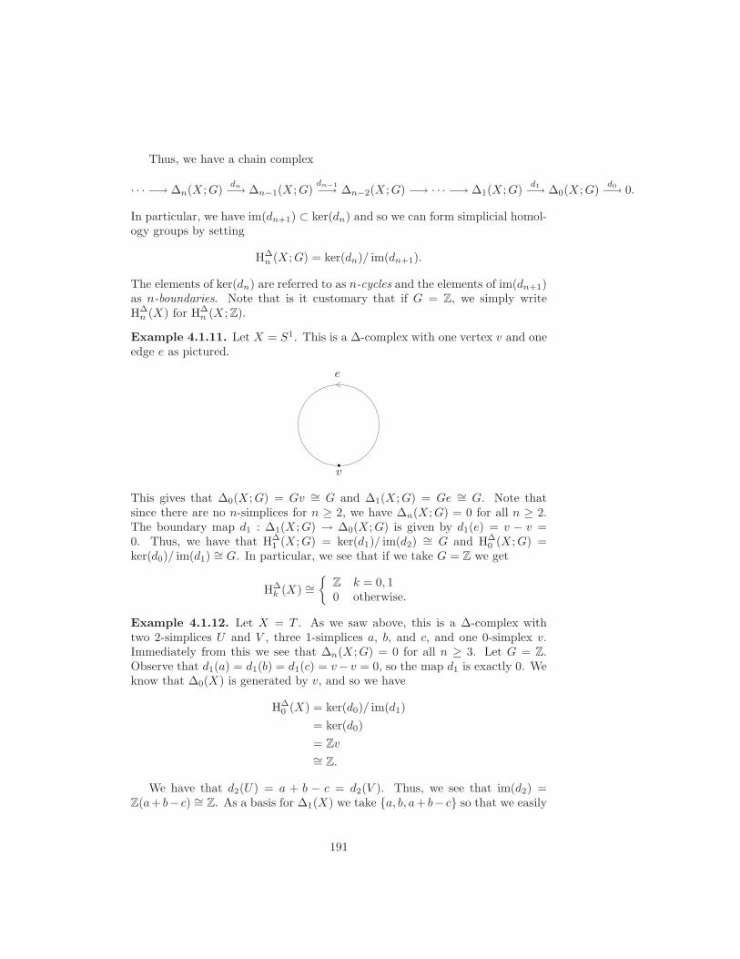
Thus, we have a chain complex

· · · −→ ∆n(X ;G)dn−→ ∆n−1(X ;G)

dn−1−→ ∆n−2(X ;G) −→ · · · −→ ∆1(X ;G)d1−→ ∆0(X ;G)

d0−→ 0.

In particular, we have im(dn+1) ⊂ ker(dn) and so we can form simplicial homol-ogy groups by setting

H∆n (X ;G) = ker(dn)/ im(dn+1).

The elements of ker(dn) are referred to as n-cycles and the elements of im(dn+1)as n-boundaries. Note that is it customary that if G = Z, we simply writeH∆n (X) for H∆

n (X ; Z).

Example 4.1.11. Let X = S1. This is a ∆-complex with one vertex v and oneedge e as pictured.

e

v

This gives that ∆0(X ;G) = Gv ∼= G and ∆1(X ;G) = Ge ∼= G. Note thatsince there are no n-simplices for n ≥ 2, we have ∆n(X ;G) = 0 for all n ≥ 2.The boundary map d1 : ∆1(X ;G) → ∆0(X ;G) is given by d1(e) = v − v =0. Thus, we have that H∆

1 (X ;G) = ker(d1)/ im(d2) ∼= G and H∆0 (X ;G) =

ker(d0)/ im(d1) ∼= G. In particular, we see that if we take G = Z we get

H∆k (X) ∼=

Z k = 0, 10 otherwise.

Example 4.1.12. Let X = T . As we saw above, this is a ∆-complex withtwo 2-simplices U and V , three 1-simplices a, b, and c, and one 0-simplex v.Immediately from this we see that ∆n(X ;G) = 0 for all n ≥ 3. Let G = Z.Observe that d1(a) = d1(b) = d1(c) = v− v = 0, so the map d1 is exactly 0. Weknow that ∆0(X) is generated by v, and so we have

H∆0 (X) = ker(d0)/ im(d1)

= ker(d0)

= Zv∼= Z.

We have that d2(U) = a + b − c = d2(V ). Thus, we see that im(d2) =Z(a+ b− c) ∼= Z. As a basis for ∆1(X) we take a, b, a+ b− c so that we easily

191

see that

H∆1 (X) = ker(d1)/ im(d2)

= (Za+ Zb+ Z(a+ b− c))/Z(a+ b − c)∼= Za⊕ Zb∼= Z⊕ Z.

Finally, since ∆3(X) = 0, we know that H∆2 (X) = ker(d2). Note that

d2(mU + nV ) = (m + n)(a + b − c). This is equal to zero precisely whenm = −n. Thus, we have that ker(d2) = Z(U − V ) ∼= Z. Thus, H∆

2 (X) ∼= Z.To summarize, we have

H∆k (X) ∼=

Z k = 0, 2Z⊕ Z k = 10 otherwise.

Exercise 4.1.13. Compute the homology groups H∆k (T ; Z/2Z).

Exercise 4.1.14. Show that the simplicial homology groups of RP2 are givenby

H∆k (RP2) ∼=

Z k = 0Z/2Z k = 10 otherwise.

One should note here that for each of the examples, there was a choiceof ∆-complex for the space X . It is natural to ask if the homology groupsdepend upon this choice. Moreover, if X and Y are homeomorphic, are thehomology groups isomorphic? What if X and Y are only homotopic? Theseare all important questions, but it turns out it is easier to work with singularhomology to answer such questions. We will study singular homology and thenshow that the singular homology groups agree with the simplicial homologygroups for any ∆-complex X .

4.2 Definitions and Basic Properties of Singular

Homology

In this section we will define and prove many of the basic properties of singularhomology. We will also show how the singular homology groups agree with thosecalculated in the previous section.

Let X be a topological space. A singular n-simplex of X is a continuous mapσ : ∆n → X . Note that we do not require this to be a nice embedding at all,only that the map is continuous. Given an abelian group G, we let Cn(X ;G)denote the free abelian group over G generated by singular n-simplices of X ,i.e. Cn(X ;G) consists of elements of the form

∑i giσi. This is huge group as

we do not put requirements such as used to define a ∆-complex on Cn(X ;G).We refer to elements of Cn(X ;G) as singular n-chains (or simply n-chains.)

192

We define the boundary maps dn : Cn(X ;G) → Cn−1(X ;G) as in § 4.1,namely,

dn(σ) =

n∑

i=1

(−1)iσ|[v0,...,vi,...,vn].

In this we are identifying ∆n−1 with [v0, . . . , vi, . . . , vn] and so σ|[v0,...,vi,...,vn] isa (n− 1)-simplex. Again we see that the boundary maps form a chain complexand so we can define singular homology groups by

Hi(X ;G) = ker(dn)/ im(dn+1).

Proposition 4.2.1. Let Xii∈I be the path-components of X. Then we have

Hi(X ;G) ∼=⊕

i∈I

Hi(Xi;G).

Proof. First, observe that since ∆n is path-connected for all n and any singularn-simplex is continuous, we have that σ(∆n) must be path-connected as well.Thus, we have that Cn(X ;G) =

⊕i∈I Cn(Xi;G). Furthermore, the definition

of the boundary map shows that it respects this decomposition. Thus, we havethat ker(dn) and im(dn+1) also decompose into direct sums, which gives theresult.

Proposition 4.2.2. We have that H0(X ;G) splits into a direct sum of copiesof G, one for each path component of X.

Proof. In light of Proposition 4.2.1, it is enough to show that if X is path-connected then H0(X ;G) ∼= G.

We know that d0 is the zero map, so H0(X ;G) = C0(X ;G)/ im(d1). Define

ε : C0(X ;G)→ G

by setting

ε

(∑

i

giσi

)=∑

i

gi.

This map is clearly surjective and a homomorphism, so it remains to show thatker(ε) = im(d1).

Let σ : ∆1 → X be a singular 1-simplex. We have

ε(d1(σ)) = ε(σ|[v1] − σ|[v0])

= 1− 1

= 0.

This gives that im(d1) ⊂ ker(ε). Suppose now that ε (∑

i giσi) = 0, i.e.,∑

i gi =0. We know that the σi’s are singular 0-simplices, so they are points ofX . Let x0

be a point in X . Choose a path γi : I → X from x0 to σi(v0), which is possiblesince X is assumed to be path-connected. Let σ0 be the singular 0-simplex with

193

image x0. Then we have that γi is a singular 1-simplex, γi : [v0, v1] → X . Wehave d1(γi) = σi − σ0. Thus,

d1

(∑

i

giγi

)=∑

i

giσi −∑

i

giσ0

=∑

i

giσi

where we have used that∑i giσ0 = σ0

∑i gi = 0. Thus, we see that if

∑i giσi ∈

ker(ε), then it is a boundary and so we have ker(ε) = im(d1) as claimed.

In the particularly easy case that X is a single point, we can calculate allthe homology groups.

Proposition 4.2.3. If X is a single point then

Hk(X ;G) ∼=

0 k > 0G k = 0.

Proof. We already know the result in the case k = 0. Observe that for each kwe have a unique singular n-simplex σn since X is a single point. In particular,we have that Cn(X ;G) ∼= G for n ≥ 0. We have dn(σn) =

∑ni=0(−1)iσn−1.

Thus, we get that dn = 0 if n is odd and σn−1 if n is even, n ≥ 0. Thus, ourchain complex becomes

· · · −→ G≃−→ G

0−→ G≃−→ G

0−→ G −→ 0.

This gives the result. Note here that we have used that the map gσn 7→ gσn−1

from Cn(X ;G) to Cn−1(X ;G) is an isomorphism to get the chain complex.

Exercise 4.2.4. It is often desirable to have all the homology groups of a pointvanish. One can accomplish this by using reduced homology. To define thereduced homology groups, use the chain complex

· · · −→ C2(X ;G)d2−→ C1(X ;G)

d1−→ C0(X ;G)ε−→ G −→ 0.

Check that this gives a chain complex. The resulting homology groups arereferred to as the reduced homology and denoted Hk(X ;G). Show that for a

spaceX one has Hk(X ;G) ∼= Hk(X ;G) for k > 0 and H0(X ;G) ∼= H0(X ;G)⊕G.

We would now like to show that homotopic spaces X and Y have isomor-phic homology groups. As the set-up mirrors what we have done before forcohomology in Chapter 3, we leave many of the verifications to exercises. Letf : X → Y be a map between topological spaces. There is an induced mapf∗ : Cn(X ;G) → Cn(Y ;G) defined by f∗(σ) = f σ and then extending lin-early.

Exercise 4.2.5. Check that the induced maps f∗ satisfy f∗dn = dnf∗.

194

· · · // Cn+1(X ;G)

f∗

dn+1 // Cn(X ;G)

f∗

dn // Cn−1(X ;G)

f∗

// · · ·

· · · // Cn+1(Y ;G)dn+1 // Cn(Y ;G)

dn // Cn−1(Y ;G) // · · · .

Thus, we have that the collection f∗ gives a chain map, i.e, the followingdiagram commutes:

Exercise 4.2.6. Show that the maps f∗ descend to maps on the homologygroups.

Exercise 4.2.7. Show that if f : X → Y and g : Y → Z are maps, then(f g)∗ = f∗ g∗.

Exercise 4.2.8. Show that id is the identity map, then id∗ = id. Be sure youunderstand what id means on each side of the equation!

Theorem 4.2.9. If maps f, g : X → Y are homotopic then the induced mapson cohomology are equal.

Proof. Our first step is to decompose ∆n×I into (n+1)-simplices. For example,if we consider the case of a 1-simplex we have

v0 v1

w0 w1

I

So in this case we see that we can break ∆1 × I into the 2-simplices [v0, v1, w1]and [v0, w0, w1]. The case of a 2-simplex can be given by

v0 v1

v2

w0w1

w2

I

In this case we see that we can break ∆2× I into the 3-simplices [v0, v1, v2, w2],[v0, v1, w1, w2], and [v0, w0, w1, w2]. More generally, let [v0, . . . , vn] = ∆n × 0

195

and [w0, . . . , wn] = ∆n × 1 with wi chosen so that wi and vi have the sameimage under the projection ∆n × I → ∆n. Our goal is to show that the unionof the (n+1)-simplices [v0, . . . , vi, wi, . . . , wn] give ∆n× I. It is easy to see thisis the case in the two examples we gave above.

For i between 0 and n − 1 define a map φi : ∆n → I by φi(t0, . . . , tn) =ti+1+· · ·+tn where this is defined in terms of barycentric coordinates. Note thatwe define φn to be 0 and φ−1 to be 1. Observe that the graph of φi is precisely then-simplex [v0, . . . , vi, wi+1, . . . , wn]. For instance, in our example above with the1-simplex we have φ0(t0, t1) = t1, which shows that [v0, v1] maps onto [v0, w1]and φ1(t0, t1) = 0 so [v0, v1] maps onto [v0, v1]. Note that φi(t0, . . . , tn) ≤φi−1(t0, . . . , tn) and so the graph of φi lies below the graph of φi−1. The regionbetween these graphs is precisely the (n+1)-simplex [v0, . . . , vi, wi, . . . , wn]. Weobtain that [v0, . . . , vi, wi, . . . , wn] is a true (n+1)-simplex since wi does not lieon the graph of φi. We have that

0 = φn(t0, . . . , tn) ≤ φn−1(t0, . . . , tn) ≤ · · · ≤ φ0(t0, . . . , tn) ≤ φ−1(t0, . . . , tn) = 1.

This shows that we get all of ∆n × I.We can now define a chain homotopy between f∗ and g∗. Let σ be a singular

n-simplex and define σ × id : ∆n × I → X × I. Let F : X × I → Y be ahomotopy between f and g. Define P : Cn(X ;G)→ Cn+1(Y ;G) by setting

Pn(σ) =

n∑

i=1

(−1)iF (σ × id)|[v0,...,vi,wi,...,wn].

We will show thatdn+1Pn − g∗ + f∗ = Pn+1dn

which gives that Pn is the chain homotopy we seek. Observe we have

dn+1Pn(σ) = dn+1

(n∑

i=1

(−1)iF (σ × id)|[v0,...,vi,wi,...,wn]

)

=∑

j≤i

(−1)j(−1)iF (σ × id)|[v0,...,vj ,...,vi,wi,...,wn]

+∑

j≥i

(−1)j+1(−1)iF (σ × id)|[v0,...,vi,wi,...,wj ,...,wn].

Observe that in the case that i = j, the terms in the two sums cancel except forthe terms F (σ × id)|[v0,w0,...,wn] and −F (σ × id)|[v0,...,vn,wn]. However, wehave that F (σ× id)|[v0,w0,...,wn] = gσ = g∗(σ) and −F (σ× id)|[v0,...,vn,wn] =−f σ = f∗(σ). Thus, we have that

dn+1Pn(σ)− g∗(σ) + f∗(σ) =∑

j<i

(−1)j(−1)iF (σ × id)|[v0,...,vj ,...,vi,wi,...,wn]

+∑

j>i

(−1)j+1(−1)iF (σ × id)|[v0,...,vi,wi,...,wj ,...,wn].

196

However, we have

Pn+1(dnσ) =∑

i<j

(−1)j(−1)iF (σ × id)|[v0,...,vi,wi,...,vj ,...,wn]

+∑

i>j

(−1)j(−1)i−1F (σ × id)|[v0,...,vj ,...,vi,wi,...,wn],

which is precisely dn+1Pn − g∗ + f∗ as desired.Thus, we have a chain homotopy between f∗ and g∗. As before, we see that

if [σ] ∈ Hn(X ;G), then we have

f∗([σ]) − g∗([σ]) = dn+1(Pn([σ])) + Pn+1(dn([σ]))

= dn+1(Pn([σ]))

= 0.

Thus, we see the maps agree on homology as claimed.

Corollary 4.2.10. If X and Y are homotopy equivalent, then Hn(X ;G) ∼=Hn(Y ;G) for all n.

Example 4.2.11. We can combine Corollary 4.2.10 along with Proposition4.2.3 to see that

Hk(Rm;G) ∼=

0 k 6= 0G k = 0.

since Euclidean space is contractible to a point by straight-line homotopy.

Let X be a topological space and A a subspace of X . We would like tobe able to relate the groups Hn(X ;G), Hn(A;G), and Hn(X/A;G) where X/Ais the quotient space as defined in Example 2.9.5 of § 2.9. In general it isvery difficult to compute homology groups straight from the definition, so wewould like to be able to relate the homology groups of X to subspaces to help usactually compute the homology groups. At first glance one might conjecture thatHn(X/A;G) ∼= Hn(X ;G)/Hn(A;G). However, this is not the case in general.Actually, it is good that this does not happen because if it did, our theorywould be useless. For instance, we can consider X as a subspace of the coneof X : CX = (X × I)/(X × 0). The cone of X is contractible and so hastrivial homology groups, which would give that all the homology groups of Xas trivial as well since X embeds into its cone. In order to get a handle on howthe homology groups of X and A are related, we define the relative homologygroups.

Let A be a subspace of X . Set Cn(X,A;G) = Cn(X ;G)/Cn(A;G). It isclear from the definition that dn restricts to a map from Cn(A;G) to Cn−1(A;G),and so we have a map dn : Cn(X,A;G)→ Cn−1(X,A;G). We again have thatdn−1 dn = 0 and so we have a chain complex

· · · −→ Cn(X,A;G)dn−→ Cn−1(X,A;G)

dn−1−→ Cn−2(X,A;G) −→ · · ·

197

which allows us to define the relative homology groups as

Hn(X,A;G) = Hn(C∗(X,A;G)).

Observe that elements of Hn(X,A;G) are represented by n-chains σ ∈ Cn(X ;G)so that dn−1(σ) ∈ Cn−1(A;G). Furthermore, a relative cycle σ ∈ Cn(X,A;G) istrivial in Hn(X,A;G) if and only if it is a relative boundary, i.e., σ = dn+1α+βfor some α ∈ Cn+1(X ;G) and some β ∈ Cn(A;G). This allows us to view thegroup Hn(X,A;G) as really the homology of X modulo the homology of A.

Exercise 4.2.12. Let i : A → X be the inclusion map and j : X → X/A theprojection map. Show that for each n ≥ 0 we have an exact sequence

0 −→ Cn(A;G)i∗−→ Cn(X ;G)

j∗−→ Cn(X,A;G) −→ 0.

As in the case of cohomology, we would like to have a long exact sequenceof homology. Observe that we have the following commutative diagram:

...

...

...

0 // Cn+1(A;G)

dn+1

i∗ // Cn+1(X ;G)

dn+1

j∗ // Cn+1(X,A;G) //

dn+1

0

0 // Cn(A;G)

dn

i∗ // Cn(X ;G)

dn

j∗ // Cn(X,A;G) //

dn

0

0 // Cn−1(A;G)

i∗ // Cn−1(X ;G)

j∗ // Cn−1(X,A;G) //

0

......

...

We have already seen that the maps i∗ and j∗ descend to maps on cohomol-ogy, so it remains to define a connecting homomorphism

∂n : Hn(X,A;G)→ Hn−1(A;G)

so that we have the following long exact sequence in homology

· · · ∂n+1−→ Hn(A;G)i∗−→ Hn(X ;G)

j∗−→ Hn(X,A;G)∂n−→ Hn−1(A;G)

i∗−→ · · · .

Let [σ] ∈ Hn(X,A;G) and let σ ∈ Cn(X,A;G) be a representative. We knowthat j∗ : Cn(X ;G)→ Cn(X,A;G) is surjective, so there exists a τ ∈ Cn(X ;G)so that j∗(τ) = σ. We have that dn(τ) ∈ Cn−1(X ;G) and the fact that the

198

diagram above commutes, we have j∗(dn(τ)) = dn(j∗(τ)) = dn(σ) = 0 becauseσ ∈ ker(dn) by assumption of it being a cycle. Thus, using the exactness ofthe (n− 1)-row we see that there exists u ∈ Cn−1(A;G) so that i∗(u) = dn(τ).Define ∂n([σ]) = [u].

Exercise 4.2.13. Check that ∂n is well-defined. Namely, show that u is a cycleand that the definition of ∂n does not depend on any of the choices made.

Exercise 4.2.14. Show that this definition of ∂n yields a long exact sequenceof homology groups as given above.

Theorem 4.2.15. Given a topological space X and a subspace A, one has thefollowing long exact sequence of homology groups

· · · ∂n+1−→ Hn(A;G)i∗−→ Hn(X ;G)

j∗−→ Hn(X,A;G)∂n−→ Hn−1(A;G)

i∗−→ · · · .

Exercise 4.2.16. Show that for any x0 ∈ X one has Hk(X, x0) ∼= Hk(X) forall k ≥ 0.

Exercise 4.2.17. Let A be a nonempty space of X . Show that the boundaryoperator ∂1 : H1(X,A;G) → H0(A;G) sends H1(X,A;G) into the subgroup

H0(A;G) of H0(A;G) and show the following sequence is exact:

· · · j∗−→ H1(X,A;G)∂1−→ H0(A;G)

i∗−→ H0(X ;G)j∗−→ H0(X,A;G) −→ 0.

Let f : X → Y be a continuous map and let A ⊂ X and B ⊂ Y besubspaces. Moreover, suppose that f(A) ⊂ B. We denote this by writingf : (X,A) → (Y,B). We have already seen that f induces a map on chainsf∗ : Cn(X ;G)→ Cn(Y ;G) by sending σ to f σ. Observe that if σ ∈ Cn(A;G),then the assumption that f(A) ⊂ B gives that f∗(σ) = f σ ∈ Cn(B;G). Thus,f∗ maps Cn(A;G) into Cn(B;G) and so f∗ gives a map on the relative chains

f∗ : Cn(X,A;G)→ Cn(Y,B;G).

Furthermore, one can easily check that this descends to a map on the relativehomology groups

f∗ : Hn(X,A;G)→ Hn(Y,B;G).

Proposition 4.2.18. If two maps f, g : (X,A)→ (Y,B) are homotopic throughmaps of pairs (X,A) and (Y,B), then

f∗ = g∗ : Hn(X,A;G)→ Hn(Y,B;G).

Proof. One uses the same argument as in the proof of Theorem 4.2.9. The samemap P works here as well.

Exercise 4.2.19. Let B ⊂ A ⊂ X be subspaces. Show that one has an exactsequence

0 −→ Cn(A,B;G) −→ Cn(X,B;G) −→ Cn(X,A;G) −→ 0.

199

Use this to show that one has a long exact sequence in homology

· · · −→ Hn(A,B;G) −→ Hn(X,B;G) −→ Hn(X,A;G) −→ Hn−1(A,B;G) −→ · · · .

We recover the long exact sequence in Theorem 4.2.15 by setting B to be asingle point.

The following theorem shows that given subspaces Z ⊂ A ⊂ X , we can“excise” the subset Z and the relative homology groups are not changed. It isknown as the Excision Theorem.

Theorem 4.2.20. (Excision Theorem) Let Z ⊂ A ⊂ X with Cl(Z) ⊂ Int(A).Then natural inclusion (X − Z,A− Z) → (X,A) induces isomorphisms

Hk(X − Z,A− Z;G) ∼= Hk(X,A;G)

for all k.

We will not prove this theorem as it is fairly long and involved. It essentiallyamounts to showing that one can compute homology groups by using simplicesthat are small. For instance, if X is a metric space, for any ǫ > 0 one can insistall the simplices lie in cubes of size ǫ. One can find a proof of this theorem inChapter 2 of [5].

Corollary 4.2.21. Let A,B be subspaces of X so that X ⊂ Int(A) ∪ Int(B).The inclusion (B,A ∩B) → (X,A) induces isomorphisms

Hk(B,A ∩B;G) ∼= Hk(X,A;G).

Proof. We reduce this to Theorem 4.2.20. Set Z = X − B. Then we haveA ∩B = A− Z. The condition that X ⊂ Int(A) ∪ Int(B) implies that Cl(Z) ⊂Int(A).

We can now relate the relative homology groups Hn(X,A;G) to the reduced

homology groups Hn(X/A;G), at least in the case that A is closed, nonemptyand is a deformation retract of an open neighborhood in X . We call such a pair(X,A) a good pair.

Proposition 4.2.22. Let (X,A) be a good pair with V an open neighborhoodof A that deformation retracts to A. Then the quotient map j induces isomor-phisms Hn(X,A;G) ∼= Hn(X/A;G) for all n.

Proof. Observe that we have the following commutative diagram

200

Hn(X,A;G) //

Hn(X,V ;G)

Hn(X −A, V −A;G)oo

Hn(X/A,A/A;G) // Hn(X/A, V/A;G) Hn(X/A−A/A, V/A −A/A;G)oo

where the horizontal maps are induced from inclusions and the vertical ones fromprojection. Since A is a deformation retract of V , we have that Hn(V,A;G) ∼=Hn(A,A;G) = 0. Thus, using Exercise 4.2.19 we see that Hn(X,A;G) ∼=Hn(X,V ;G). Furthermore, we see that Hn(X/A,A/A;G) ∼= Hn(X/A, V/A;G)by the exact same argument since V/A retracts to A/A. Thus, both of the lefthorizontal arrows are isomorphisms. We obtain that the horizontal right twoarrows are isomorphisms from Theorem 4.2.20.

Observe that the projection map j : X → X/A is a homeomorphism when werestrict to X−A, namely, j : X−A→ X/A−A/A is a homeomorphism. Thus,the right vertical arrow is an isomorphism. One can now use the commutativityof the diagram to see that the left-most vertical arrow is an isomorphism aswell. Thus, we have that

Hn(X,A;G) ∼= Hn(X/A,A/A;G).

However, we know that A/A is a single point so Exercise 4.2.16 gives that

Hn(X/A,A/A;G) ∼= Hn(X/A;G) as desired.

Corollary 4.2.23. We have

Hk(Sn;G) ∼=

G k = n,0 k 6= n.

Proof. Let X = Dn = x ∈ Rn : |x| ≤ 1 and A = Sn−1 so that A = ∂X .Observe that X/A ∼= Sn. (Be sure you understand why!) The fact that Dn is

contractible gives Hk(Dn;G) = 0 for all k. We apply the long exact sequence

given in Exercise 4.2.17 to obtain

0 −→ Hk(Dn, Sn−1;G) −→ Hk−1(S

n−1;G) −→ 0,

for k > 1 and

0 −→ H1(Dn, Sn−1;G) −→ H0(S

n−1;G) −→ 0.

Thus we have that

Hk(Dn, Sn−1;G) ∼= Hk−1(S

n−1;G)

for all k where we have used the homology and reduced homology groups agreefor k > 0. We have that (Dn, Sn−1) is a good pair, so Proposition 4.2.22 givesthat

Hk(Dn, Sn−1;G) ∼= Hk(S

n;G).

201

Combining these results we see that

Hk(Sn;G) ∼= Hk−1(S

n−1;G).

Observing that S0 consists of two points, we obtain the result by using Propo-sitions 4.2.1 and 4.2.3 and induction.

Exercise 4.2.24. Use this to give alternative proofs of Lemma 3.4.28 and The-orem 3.4.27.

Example 4.2.25. We can construct explicit generators of the groups Hn(Dn, ∂Dn)

and Hn(Sn) that will be useful to know. First we deal with Hn(Dn, ∂Dn). Ob-

serve that we can replace the pair by (∆n, ∂∆n) since they are homotopy equiv-alent. We claim that the identity map id : ∆n → ∆n when viewed as a singularn-simplex is a cycle generating Hn(∆n, ∂∆n). We proceed by induction. Thecase n = 0 is clear. Let Λ ⊂ ∆n be the union of all but one of the (n − 1)dimensional faces of ∆n. Observe that we have an isomorphism

Hn(∆n, ∂∆n)

≃−→ Hn−1(∂∆n,Λ)

that arises from considering the triple in Exercise 4.2.19 as (∆n, ∂∆n,Λ) andusing that Hn(∆

n,Λ) = 0 since ∆n deformation retracts onto Λ and so (∆n,Λ)is homotopy equivalent to (Λ,Λ). We also have an isomorphism

Hn−1(∆n−1, ∂∆n−1)

≃−→ Hn−1(∂∆n).

To obtain this isomorphism, observe that the inclusion ∆n−1 → ∂∆n of theface not contained in Λ induces a homeomorphism of quotients ∆n−1/∂∆n−1 ∼=∂∆n/Λ. One then uses that the pairs being considered are good pairs alongwith Proposition 4.2.22 to obtain the isomorphism. We now have the result byinduction since the cycle id is sent under the first isomorphism to ∂ id, whichequals ± id in Cn−1(∂∆n,Λ).

We can now regard Sn as two n-simplices ∆n1 and ∆n

2 with the boundariesidentified in the obvious way. We can then view the difference ∆n

1 − ∆n2 as a

singular n-chain that is a cycle. We claim this generates Hn(Sn) for n > 0.

Using the long exact sequence for the pair (Sn,∆n2 ) we obtain an isomorphism

Hn(Sn)≃−→ Hn(S

n,∆n2 ).

We can also use the same argument given above with quotients to obtain anisomorphism

Hn(∆n1 , ∂∆n

1 )≃−→ Hn(S

n,∆n2 ).

Under these isomorphisms, the cycle ∆n1 −∆n

2 in the group Hn(Sn) corresponds

to the cycle ∆n1 in the group Hn(∆

n1 , ∂∆n

1 ), which represents a generator of this

group. Thus, we have that ∆n1 −∆n

2 is a generator of the group Hn(Sn).

202

When studying topology, there is always the issue of picking the “right”spaces to study. For instance, if we try and be too general it will be difficult toprove any interesting theorems. Of course, we would like to be as general as isreasonably possible to encompass as many spaces as we can. In studying singularhomology, the “right” spaces are generally CW-complexes. A CW-complex isbuilt up inductively. We call a set a n-cell if it is homeomorphic to Un =x ∈ Rn : |x| < 1. Let Y be a Hausdorff space and X a closed subspace of Y .Suppose that Y −X consists of a disjoint union of n-cells eni i∈I . Furthermore,assume that for each i ∈ I there is a continuous map fi : Dn → Cl(en) so thatfi maps Un homeomorphically onto en and fi(S

n−1) ⊂ X . If I is a finite set, wesay Y is obtained from X by attaching n-cells. If I is not finite, we require thatY has the weak topology determined by the maps fi and the inclusion X → Y .The weak topology condition means that A ⊂ Y is closed if and only if A ∩Xis closed and the sets f−1

i (A) are closed for all i ∈ I.

Definition 4.2.26. A structure of a CW-complex is prescribed on a Hausdorffspace X by an ascending chain of closed subspaces

X0 ⊂ X1 ⊂ · · ·

that satisfy:

1. X0 has the discrete topology

2. For n > 0, Xn is obtained from Xn−1 by attaching a collection of n-cellsas described above.

3. X is the union of X i for i ≥ 0.

4. The space X and the subspacesX i all have the weak topology: A subset Ais closed if and only if A∩Cl(en) is closed for all n-cells en for n = 0, 1, . . . .

We call the subset X0 of X the vertices. The subset Xn is the n-skeleton of X .We say X is finite or infinite according to whether the number of cells is finiteor infinite. If X = Xn we say X is finite dimensional and call n the dimensionof X .

Definition 4.2.27. A subset A of a CW-complex X is called a subcomplex ifA is the union of cells of X , and if for any cell en we have that en ⊂ A impliesthat Cl(en) ⊂ A.

In fact, if A is a subcomplex of X then the sets An = A ∩ Xn define aCW-complex structure on A. It is a fact that if A ⊂ X is a subcomplex of aCW-complex X , then (X,A) is a good pair. One can see Appendix A of [5] fora proof of this fact and many others about the basic topology of CW-complexes.

Definition 4.2.28. A continuous map f : X → Y of CW-complexes is calledcellular if f(Xn) ⊂ Y n for n ≥ 0.

203

Example 4.2.29. Let X = Sn. Then X is a CW-complex with one e0 and oneen. For instance, the case n = 2 is given by identifying the boundary of the openunit disc U2 to a point, which gives the sphere. In particular, for 0 ≤ k < n,Xk consists of a single point and Xn = Sn and the map that attaches en toXn−1 is by mapping the boundary of Dn to a point.

Example 4.2.30. Let X be a 1-dimensional CW-complex. Then X consists ofvertices and edges, 0-cells and 1-cells. This is a graph.

Example 4.2.31. The ∆-complexes given in § 4.1 are CW-complexes. Notethat for n ≥ 1, Int(∆n) is homeomorphic to Un. Thus, we have that the torus,RP2, and the Klein bottle are all CW-complexes.

Example 4.2.32. Consider RPn. Observe that RP0 is just a point. We alsohave that RP1 is the circle. For instance, one can see this via the map

[x : y] 7→(

x√x2 + y2

,y√

x2 + y2

).

We can use these base skeletons to build RPn. We proceed by induction. Sup-pose that we have constructed RPn−1. We can build RPn from RPn−1 byadjoining a single n-cell. We define the map

fn : Dn → RPn

by settingfn(x1, . . . , xn) = [x1 : · · · : xn :

√1− |x|2]

where x = (x1, . . . , xn). It now straight-forward to check that fn maps Dn −Sn−1 homeomorphically onto RPn−RPn−1 and maps Sn−1 onto RPn−1, thoughnot homeomorphically. Thus, we have that RPn is a CW-complex with one cellof each dimension, i.e., RPn = e0 ∪ e1 ∪ · · · ∪ en.

Exercise 4.2.33. Show that CPn is a CW-complex with decomposition CPn =e0 ∪ e2 ∪ e4 ∪ · · · ∪ e2n.

We have the excision property for subcomplexes of CW-complexes as well.

Corollary 4.2.34. If the CW-complex X is the union of subcomplexes A andB, then the inclusion map (B,A ∩B)→ (X,A) induces isomorphisms

Hn(B,A ∩B;G) ∼= Hn(X,A;G)

for all n.

Proof. We know that all CW-pairs are good pairs, and so we can use Proposition4.2.22 to pass to the quotient spaces B/A ∩ B and X/A. These spaces arehomeomorphic since X = A ∪B, and so we have the result.

204

The wedge sum is a useful operation when studying CW-complexes. Let Xand Y be topological spaces and let x0 ∈ X , y0 ∈ Y . We define the wedge sumX ∨ Y of X and Y with respect to x0 and y0 to be the quotient of the disjointunion of X and Y obtained by identifying x0 and y0. More generally, we candefine a wedge sum of an arbitrary collection of spaces Xi with respect to pointsxi ∈ Xi for i ∈ I by forming the quotient space of the disjoint union of the Xi

by identifying the xi to a single point. We denote this space by ∨i∈IXi.

Example 4.2.35. The wedge sum S1 ∨ S1 is a figure eight.

Example 4.2.36. Consider the set X0 = e01, e02, e03. Attach two 1-cells e11 ande12 to form X1 as in the following picture:

e01

e02

e03

e11e12

Consider the quotient space X1/X0. Note we identify all the vertices to onepoint, say v. We have the picture:

v

e11 e12

Note that X1/X0 is homeomorphic to S1 ∨ S1.More generally, if Xn is a n-skeleton formed from Xn−1 by attaching n-cells,

then Xn/Xn−1 is homeomorphic to the wedge sum of copies of Sn, one copyfor each n-cell attached.

We will return to CW-complexes in § 4.4. We finish this section by provingthat the simplicial and singular homology groups agree for a ∆-complexX . Thiswill give us the singular homology groups of the examples calculated in § 4.1. LetX be a ∆-complex and A a subcomplex, i.e., A is a ∆-complex formed via theunion of simplicies in X . We can define relative simplicial homology groups bysetting ∆k(X,A;G) = ∆k(X ;G)/∆n(A;G). As in the singular case this gives achain complex and so we define the relative simplicial homology groups via thatchain complex. We obtain a long exact sequence of simplicial homology groups

205

as in Theorem 4.2.15. There is a natural map ∆k(X,A;G)→ Ck(X,A;G). Notewe include the case A = ∅ to recover the natural map ∆k(X ;G) → Ck(X ;G).This natural map induces a map on homology H∆

k (X,A;G) → Hk(X,A;G).Note that a ∆-complex X is certainly a CW-complex as well.

Theorem 4.2.37. The homomorphisms H∆k (X,A;G) → Hk(X,A;G) are iso-

morphisms for all k and all ∆-complex pairs (X,A).

Proof. We begin with the case that X is finite dimensional and A is empty. Wehave the following commutative diagram of exact sequences:

H∆n+1(X

k, Xk11) //

H∆n (Xk−1) //

H∆n (Xk) //

H∆n (Xk, Xk11) //

H∆n−1(X

k−1)

Hn+1(X

k, Xk−1) // Hn(Xk−1) // Hn(Xk) // Hn(X

k, Xk−1) // Hn−1(Xk−1).

Note that we drop the G from the notation here to save space, but the resultfollows with coefficients as well.

We have that ∆n(Xk, Xk−1;G) is zero for n 6= k and is a free abelian group

generated by the k-simplices when k = n. Thus, we have that H∆n (Xk, Xk−1;G)

is zero for n 6= k and is free abelian generated by the k-cycles for n = k. Con-sider the map Ψ :

∐i(∆

ki , ∂∆k

i ) −→ (Xk, Xk−1) given by the maps ∆k → Xfor each k-simplex. We have that Ψ gives a homeomorphism of the spaces∐i ∆

ki /∐i ∂∆k

i with Xk/Xk−1, and so induces an isomorphism of singular ho-mology groups. This shows that Hn(X

k, Xk−1;G) is zero for n 6= k. Forn = k we have that it is free abelian with basis the relative cycles givenby characteristic maps of the k-simplices of X since Hk(∆

k, ∂∆k;G) is gen-erated by the identity map ∆k −→ ∆k (check this). Thus, we have the mapH∆k (Xk, Xk−1;G) −→ Hk(X

k, Xk−1;G) is an isomorphism. This gives that thefirst and fourth vertical maps in the commutative diagram above are isomor-phisms. We may assume the second and fifth vertical maps are isomorphismsby induction, so the Five Lemma gives that the middle one is an isomorphismas well. This gives the result in this case.

Suppose now that X is infinite dimensional. One has that a compact setin X can only meet finitely many open simplices of X . One can see AppendixA of [5] for a proof of this fact. We will encounter it again when we continueour study of CW-complexes. In the case of a ∆-complex it is even easier andshould be proved as an exercise. Let [z] ∈ Hn(X ;G) with z a representative inCn(X ;G). By definition this is a linear combination of finitely many singularsimplices with compact images, so it must be contained in Xk for some k. Sincewe already have that H∆

n (Xk;G) → Hn(Xk;G) is an isomorphism for all n,

we have that z is homologous to a simplicial cycle. Thus, we have that themap H∆

n (X ;G)→ Hn(X ;G) is surjective. Now suppose that [σ] ∈ H∆n (X ;G) is

represented by σ ∈ ∆n(X ;G) and it is the boundary of a singular chain inX . Weknow this chain must have compact image, and so is contained in Xk for some

206

k. Thus, σ represents an element in the kernel of H∆n (Xk;G) → Hn(X

k;G),which is trivial. Thus, σ must be a simplicial boundary and we are done.

One can do the case when A 6= ∅ by the same method as above if onereplaces the commutative diagram with the corresponding commutative diagramof relative homology and simplicial homology groups.

An efficient way for computing the homology groups of a CW complex is viacellular homology, which we introduce after a few basic definitions and facts.

The following corollary of Proposition 4.2.22 will also be necessary in com-puting the homology of CW complexes.

Corollary 4.2.38. Let Xk be a collection of topological spaces and ∨kXk thewedge sum. The inclusion maps ik : Xk −→ ∨kXk induce an isomorphism

⊕k(ik)∗ :⊕

k

Hn(Xk) −→ Hn(∨kXk)

assuming that the wedge sum is formed with respect to base points xk so that(Xk, xk) is a good pair.

Proof. Consider the pair (∐kXi,

∐kxk). We have that

Hn

(∐

k

Xk,∐

k

xk)∼=⊕

k

Hn(Xk, xk)

∼=⊕

k

Hn(Xk).

On the other hand, Proposition 4.2.22 gives that

Hn

(∐

k

Xk,∐

k

xk)∼= Hn(∨kXk).

Combining these gives the result.

Lemma 4.2.39. Let X be a CW complex.

1. Hn(Xk, Xk−1) = 0 for n 6= k and is free abelian for n = k with a basis in

one to one correspondence with the n-cells of X.

2. Hn(Xk) = 0 for n > k. In particular, if X is finite dimensional then

Hn(X) = 0 for n > dimX.

3. The inclusion map i : Xk → X induces an isomorphism i∗ : Hn(Xk) →

Hn(X) if n < k.

Proof. 1. Observe that (Xk, Xk−1) is a good pair and Xk/Xk−1 is a wedgesum of k-spheres. We now use Corollary 4.2.38 combined with our previouscalculations of the homology of spheres to get the result.

207

2. Consider the long exact sequence arising from the pair (Xk, Xk−1). Inthis exact sequence we have

Hn+1(Xk, Xk−1) −→ Hn(X

k−1) −→ Hn(Xk) −→ Hn(X

k, Xk−1).

If n 6= k, k−1, then the outer two groups are 0 and so we have Hn(Xk−1) ∼=

Hn(Xk) for all n 6= k, k − 1. Thus, if n > k then we have Hn(X

k) ∼=Hn(X

k−1) ∼= · · · ∼= Hn(X1) ∼= Hn(X0) = 0. This proves the second part.

3. Note that we can use what we have just shown in the case that X isfinite dimensional to conclude that if n < k then Hn(X

k) ∼= Hn(Xk+1) ∼=

· · · ∼= Hn(Xk+m) for all m ≥ 0, which gives the third result if X is finite

dimensional. In the case that X is not finite dimensional, we use the sameargument we’ve used before to observe that any singular n-chain in Xhas compact image so sits inside Xm for some m. Thus, a n-cycle in Xis homologous to a cycle in Xk if k > n by the finite dimensional case.Thus, the induced map i∗ : Hn(X

k) → Hn(X) is surjective. Similarly, ifa n-cycle in Xk bounds a chain in X , this chain lies in Xm for some mwith m ≥ k, so by the finite dimensional case the cycle bounds a chain inXk if k > n.

We can now build the cellular chain complex which can be very useful incomputing homology groups of CW complexes. Consider the following diagram:

0

0

''PPPPPPPPPPPPPP Hn(Xn+1)

≃ //

66mmmmmmmmmmmmmmmHn(X)

Hn(Xn)

jn

''OOOOOOOOOOO

in

77ooooooooooo

· · · // Hn+1(Xn+1, Xn)

∂n+1

77nnnnnnnnnnnn jn∂n+1 // Hn(Xn, Xn+1)

∂n ((QQQQQQQQQQQQ

jn−1∂n // Hn−1(Xn−1, Xn−2) // · · ·

Hn−1(Xn−1)

jn−1

55lllllllllllll

0

66mmmmmmmmmmmmmmm

Observe that the composition of two of the maps in the horizontal part ofthe diagram consists of at two successive maps in one of the diagonal exact

208

sequences, so must be zero. Thus, the horizontal row gives a chain complex.This complex is known as the cellular chain complex. We denote the homologygroups of this chain by HCW

n (X).

Theorem 4.2.40. One has HCWn (X) ∼= Hn(X) for all n.

Proof. To ease the notation write dCWn for jn−1 ∂n. Observe that we have

Hn(X) ∼= Hn(Xn)/ ker(in) ∼= Hn(X

n)/ im(∂n+1).

The fact that jn is injective gives that im(∂n+1) maps isomorphically ontoim(jn∂n+1) = im(dCW

n+1). Furthermore, we see that Hn(Xn) maps isomorphi-

cally onto im(jn) = ker(∂n). We have that jn−1 is injective, so ker(∂n) =ker(dCW

n ). Thus, the map jn induces an isomorphism between the quotientHn(X

n)/ im(∂n+1) and ker(dCWn )/ im(dCW

n+1), which gives the result.

Corollary 4.2.41. If X is a CW complex with k n-cells, then Hn(X) is gen-erated by at most k elements. In particular, if there are no n-cells in X thenHn(X) = 0.

Proof. We know that Hn(Xn, Xn−1) is a free abelian group generated by the n-

cells. Thus, we must have that the kernel of dCWn is generated by at most these

k n-cells. Thus, HCWn (X) ∼= Hn(X) is generated by at most k elements.

Corollary 4.2.42. Let X be a CW complex that has no two of its cells inadjacent dimensions. Then Hn(X) is free abelian with basis in one to one cor-respondence with the n-cells of X. In particular, this gives

Hk(CPn) =

Z for k = 0, 2, 4, · · · , 2n0 otherwise.

Proof. This is clear because in this case all of the maps dCWn must be 0.

Another nice application we have is to the Euler characteristic of a finiteCW complex. Define the Euler characteristic of a finite CW complex X to be

χ(X) =∑

n

(−1)ncn

where cn is the number of n-cells of X . Note that this is a generalization ofthe familiar formula for 2-complexes that reads χ(X) is the number of vertices- number of edges + number of faces. In fact, we can now see that χ(X) canbe defined completely in terms of the homology of X and so is a homotopyinvariant of the space.

Theorem 4.2.43. For X a finite CW complex one has

χ(X) =∑

n

(−1)n rank(Hn(X)).

209

Proof. This result is a purely algebraic result. Let

0 −→ Ckdk−→ Ck−1 −→ · · · −→ C1

d1−→ C0 −→ 0

be a descending chain complex of finitely generated abelian groups. DefiningZn, Bn, and Hn(C∗) as always, we have short exact sequences

0 −→ Zn −→ Cn −→ Bn−1 −→ 0

and0 −→ Bn −→ Zn −→ Hn(C∗) −→ 0.

We now apply the fact that if

0 −→ A −→ B −→ C −→ 0

is a short exact sequence of finitely generated abelian groups, then rank(B) =rank(A) + rank(C) to obtain that

rank(Cn) = rank(Zn) + rank(Bn−1)

= rank(Bn) + rank(Hn(C∗)) + rank(Bn−1).

If we multiply this equation by (−1)n and sum over all n we obtain

∑

n

(−1)n rank(Cn) =∑

n

(−1)n rank(Hn(C∗)).

Now just apply this purely algebraic result to the complex Cn = Hn(Xn, Xn−1)

to get the result.

4.3 The Universal Coefficient Theorem

In § 4.2 we saw that working with homology with coefficients in an arbitraryabelian group did not add any difficulties in proving theorems. It can be thecase that using arbitrary coefficients can make working examples a little trickier,but essentially it did not appear anything new was gained or lost by switchingfrom G to Z or vice versa. In this section we justify that statement by relatingthe homology groups Hk(X,A;G) to Hk(X,A) ⊗ G. Note when a subscript isnot added to the tensor product it is understood to be a tensor product overZ. One of the main reasons for interest in such a result for us is to prepare usfor the same result when we introduce cohomology. In that context a universalcoefficient theorem will be important when we compare different cohomologytheories.

Let X be a topological space and G an abelian group. Recall that Cn(X ;G)is the free abelian group over G generated by the chains σ : ∆n → X . Inparticular, given a chain τ ∈ Cn(X ;G), we can write τ =

∑i giσi for σi : ∆n →

X singular n-simplices. From this it is clear that we have

Cn(X ;G) ∼= Cn(X)⊗G

210

where the map is given by∑i giσi maps to

∑i σi ⊗ gi. From this we see that

we can write our chain complex

· · · −→ Cn(X ;G)dn−→ Cn−1(X ;G)

dn−1−→ Cn−2(X ;G) −→ · · ·

as

· · · −→ Cn(X)⊗G dn⊗1−→ Cn−1(X)⊗G dn−1⊗1−→ Cn−2(X)⊗G −→ · · · .

Thus, the homology groups we defined relative to Cn(X ;G) can also be givenas the homology groups of this chain complex, namely,

Hn(X ;G) = Hn(C∗(X)⊗G).

The group G is referred to as the coefficients of the homology group. We canview the relative homology groups in this way as well, in particular, Cn(X,A;G) ∼=Cn(X,A)⊗G.

Before we relate Hn(X,A;G) to Hn(X,A) ⊗ G, we consider the inducedhomomorphisms Hn(X,A;G) → Hn(X,A;H) when we have a homomorphismbetween the groups G and H . Let φ : G → H be a group homomorphism.Clearly, we have an induced homomorphism on chains given by

1⊗ φ : Cn(X,A)⊗G −→ Cn(X,A)⊗H.

These maps descend to maps on homology, though to avoid confusion we addsome details here. (Note that we do not have that Hn(X,A;G) ∼= Hn(X,A)⊗G!)Let [τ ] ∈ Hn(X,A;G) and let τ =

∑i σi⊗gi ∈ Cn(X,A)⊗G be a representative

of [τ ]. We have that (1⊗φ)(τ) =∑i σi ⊗φ(gi) ∈ Cn(X,A)⊗H . It is therefore

natural to define

φ♯ : Hn(X,A;G)→ Hn(X,A;H)

[τ ] 7→ [(1 ⊗ φ)(τ)].

There are two things to check. The first is that the image of this map is actuallya cycle, and the second is that it does not depend on the choice of representativefor [τ ]. To see the image is a cycle, observe that

(dn ⊗ 1)

(∑

i

σi ⊗ φ(gi)

)=∑

i

dn(σi)⊗ φ(gi)

= (1 ⊗ φ)

(∑

i

dn(σi)⊗ gi)

= (1 ⊗ φ)(0)

= 0

where we have used that∑

i dn(σi) ⊗ gi = 0 because τ is a cycle and thatφ is a homomorphism so takes 0 to 0. Thus, we have that the image lies inHn(X,A;H).

211

Exercise 4.3.1. Check that if one chooses different representatives of [τ ] thatthey are mapped to the same thing in Hn(X,A;H).

For this induced map to be useful it is important that the map is “natural”,i.e., it commutes with the induced maps we have already defined. Namely, givena continuous map f : (X,A)→ (Y,B) and a group homomorphism φ : G→ H ,it is important that the following diagram commutes:

Hn(X,A;G)f∗ //

φ♯

Hn(Y,B;G)

φ♯

Hn(X,A;H)

f∗ // Hn(Y,B;H).

However, this follows immediately from the definitions. It is also important thatthe induced map φ♯ behaves well with respect to the boundary homomorphism∂n. In particular, we have that the following diagram commutes:

Hn(X,A;G)∂n //

φ♯

Hn−1(A;G)

φ♯

Hn(X,A;H)

∂n // Hn−1(A;H).

Again, one only needs to write down the definitions of the maps to see that thisis true.

This induced map has many important uses in homology theory. For exam-ple, let R be a ring and suppose that G is a R-module. We write the action ofR on G as left multiplication. Thus, for each r ∈ R we have an endomorphismof G given by g 7→ rg. Using what we have just shown, each r ∈ R induces amap r♯ of Hn(X,A;G).

Exercise 4.3.2. Show that the induced maps r♯ give the group Hn(X,A;G) thestructure of a R-module. Furthermore, show that the commutative diagramsabove show that f∗ and ∂n are homomorphisms of R-modules.

A particularly nice case is when R is a field and G is a vector space overR. In this case one has that Hn(X,A;G) is a vector space over R as well andthe maps f∗ and ∂n are linear transformations. What makes this situationparticularly nice is that one can then use all the tools of linear algebra to studythe homology groups.

We now return to studying the relation between Hn(X,A;G) and Hn(X,A)⊗G. In order to do this we introduce some definitions and results from generalhomological algebra.

212

Definition 4.3.3. Let A,B, and C be abelian groups with

0 −→ Ai−→ B

j−→ C −→ 0

an exact sequence. We say the exact sequence splits if there is an isomorphismB ∼= A⊕ C that makes the following diagram commutewhere the maps A→ A⊕C is the natural inclusion map and the map A⊕C → C

B

∼=

j

##FFF

FFFF

FF

0 // A

i

;;xxxxxxxxx

""FFF

FFFF

FF C // 0

A⊕ C

;;xxxxxxxxx

is the natural projection map.

Exercise 4.3.4. Show that if A,B, and C are free abelian groups then everyshort exact sequence is split. In fact, given a short exact sequence, show it isenough for C to be free for the short exact sequence to split.

Lemma 4.3.5. Let A,B, and C be abelian groups and

0 −→ Ai−→ B

j−→ C −→ 0

a split short exact sequence. Given any abelian group G, the sequence

0 −→ A⊗G i⊗1−→ B ⊗G j⊗1−→ C ⊗G −→ 0

is a split exact sequence.

Proof. First, observe that the tensor product operation is right exact, namely,we get that

A⊗G i⊗1−→ B ⊗G j⊗1−→ C ⊗G −→ 0

is exact for any exact sequence

0 −→ Ai−→ B

j−→ C −→ 0.

To get the injectivity of the first map, observe that

(A⊕ C)⊗G ∼= (A⊗G)⊕ (C ⊗G)

and so clearly the inclusion map

A⊗G→ (A⊗G)⊕ (C ⊗G)

is injective. This gives the injectivity since the sequence is split. It is also clearnow that the sequence

0 −→ A⊗G i⊗1−→ B ⊗G j⊗1−→ C ⊗G −→ 0

is split.

213

Let Cn, dn be a descending chain complex of free abelian groups, i.e., achain complex given as

· · · −→ Cn+1dn+1−→ Cn

dn−→ Cn−1 −→ · · ·

with each Cn a free abelian group. Set Zn = ker(dn) ⊂ Cn and Bn =im(dn+1) ⊂ Cn. We can define the homology group of Cn as

Hn(C∗) = Zn/Bn.

We have the following commutative diagram

...

...

...

0 // Zn

dn

// Cndn //

dn

Bn−1

dn−1

// 0

0 // Zn−1

// Cn−1dn−1 //

Bn−2

// 0

......

...

where each horizontal row is exact. Observe that each row is split because Bnis free as it is a subgroup of the free abelian group Cn. Let G be any abeliangroup. Lemma 4.3.5 combined with the above commutative diagram gives usan exact sequence of chain complexes

0 −→ Z∗ ⊗G −→ C∗ ⊗G −→ B∗−1 ⊗G −→ 0.

This gives a long exact sequence of homology groups

· · · −→ Hn+1(B∗⊗G) −→ Hn(Z∗⊗G) −→ Hn(C∗⊗G) −→ Hn(B∗⊗G) −→ · · · .

However, we know that dn ⊗ 1 maps all elements of Zn ⊗G and Bn ⊗G to 0,so Hn(Z∗ ⊗ G) = Zn ⊗G and Hn(B∗ ⊗ G) = Bn−1 ⊗G. Thus, the long exactsequence becomes

(4.1) · · · −→ Bn ⊗G −→ Zn ⊗G −→ Hn(C∗ ⊗G) −→ Bn−1 ⊗G −→ · · · .

The connecting homomorphism ∂n+1 : Hn+1(B∗⊗G)→ Hn(Z∗⊗G) is the mapin ⊗ 1 : Bn ⊗ G → Zn ⊗ G where in is the inclusion map. One should checkthis as an exercise. We break up the long exact sequence (4.1) into short exactsequences

(4.2) 0 −→ coker(in ⊗ 1) −→ Hn(C∗ ⊗G) −→ ker(in−1 ⊗ 1) −→ 0.

214

Consider the short exact sequence defining Hn(C∗), namely,

0 −→ Bnin−→ Zn

jn−→ Hn(C∗) −→ 0.

As was stated above, it is a fact from commutative algebra that tensoring withG is right exact so we have the exact sequence

Bn ⊗G in⊗1−→ Zn ⊗G jn⊗1−→ Hn(C∗)⊗G −→ 0.

In particular, we see that

Hn(C∗)⊗G ∼= (Zn ⊗G)/ ker(jn ⊗ 1)∼= (Zn ⊗G)/ im(in ⊗ 1)

= coker(in ⊗ 1).

Thus, we can rewrite the short exact sequence (4.2) as

0 −→ Hn(C∗)⊗G −→ Hn(C∗ ⊗G) −→ ker(in−1 ⊗ 1) −→ 0.

It remains to study ker(in−1 ⊗ 1). This requires a little more background andwork.

Definition 4.3.6. Let H be an abelian group. A free resolution F∗ = Fi, fiof H is an exact sequence

· · · −→ F2f2−→ F1

f1−→ F0f0−→ H −→ 0

where each Fi is a free abelian group.

We know that if we tensor the free resolution of H with an abelian group Gthe resulting sequence is not necessarily exact. We define

Hn(F∗ ⊗G) = ker(fn ⊗ 1)/ im(fn+1 ⊗ 1).

This group only depends upon G and H and not the free resolution F∗ used aswe will see in Lemma 4.3.8. First, we need the following result on chain mapsof free resolutions.

Lemma 4.3.7. Let E∗ a free resolution of an abelian group G and F∗ be afree resolution of an abelian group H. Then every homomorphism φ : G → Hextends to a chain map from E∗ to F∗, i.e., the following diagram commutes

215

· · · // E2

φ2

e2 // E1

φ1

e1 // E0

φ0

e0 // G //

φ

0

· · · // F2f2 // F1

f1 // F0f0 // H // 0.

Moreover, any two such chain maps extending φ are chain homotopic.

Proof. We construct the maps φi inductively. It is enough to define φi on a basisof Ei since Ei is free. Let x ∈ E0 be a basis element. Since f0 is surjective,there exists a y ∈ F0 so that f0(y) = φ(e0(x)). Define φ1(x) = y. This definesφ0. We would like to define φ1 in the same manner. Let x now be a basiselement in E1. We want to find y ∈ F1 so that f1(y) = φ0(e1(x)). We seethat such a y will exist if φ0(e1(x)) ∈ im(f1) = ker(f0). However, we have thatφ0(e1(x)) ∈ ker(f0) because φ0(e1(X)) = φ(e0(e1(x))) = φ(0) = 0. Thus, wecan define φ1 as desired. The rest of the maps are defined in the same manner.

Now suppose there is another chain map φ′ : E∗ → F∗ extending φ. Considerthe maps ψi : Ei → Fi defined by ψi = φi − φ′i. This is a chain map extendingthe zero map from G to H . It is enough to show that ψi is chain homotopicto 0, i.e., to construct maps Ti : Ei → Fi+1 so that ψi = fi+1Ti + Ti−1ei.We construct the maps Ti inductively much as the maps φi were constructed.For i = 0, set T−1 : G → F0 to be the zero map. The relation we need inthis case is ψ0 = f1T0. Define T0 as follows. Let x ∈ E0 a basis element.Note that there is a y ∈ F1 so that f1(y) = ψ0(x) because im(f1) = ker(f0) andf0(ψ0(x)) = ψ(e0(x)) = 0 since ψ is the zero map. Thus, we can define T0(x) = yand this gives the desired relation. Now we show the inductive step. We needto define Ti so that it takes a basis element x ∈ Ei to a basis element y ∈ Fi+1sothat fi+1(y) = ψi(x) − Ti−1ei(x). This is possible if ψi(x) − Ti−1ei(x) lies inim(fi+1) = ker(fi), i.e, if fi(ψi − Ti−1ei) = 0. However, using the relationsfiψi = ψi−1ei and ψi−1 = fiTi−1 + Ti−2ei−1 (which holds by our inductionhypothesis), we have

fi(ψi − Ti−1ei) = fiψi − fiTi−1ei

= ψi−1ei − fiTi−1ei

= (ψi−1 − fiTi−1)ei

= Ti−1ei−1ei

= 0.

Thus, we have the result.

Lemma 4.3.8. Let E∗ and F∗ be two free resolutions of H. For each n thereis a canonical isomorphism

Hn(E∗ ⊗G) ∼= Hn(F∗ ⊗G).

Proof. Let E∗ and F∗ be two free resolutions of H . We tensor these free reso-lutions with G to obtain chain complexes E∗⊗G and F∗⊗G with maps φn⊗ 1

216

giving the chain map between them. These maps descend to maps on homology

φ∗ : Hn(E∗ ⊗G)→ Hn(F∗ ⊗G).

Note that the maps on homology are independent of the chain maps φ∗ as ifone has a different sent of chain maps, we have that they are chain homotopic,which in homology means they agree.

Suppose that we have a composition H1φ−→ H2

ψ−→ H3 with free reso-lutions F∗, F

′∗, and F ′′

∗ respectively. The induced maps on homology satisfy(ψφ)∗ = ψ∗φ∗. One can see this by choosing the chain map F∗ → F ′′

∗ to bethe composition of chain maps F∗ → F ′

∗ → F ′′∗ . Now if φ is an isomorphism

and ψ the inverse of φ, then we have ψ∗φ∗ = (ψφ)∗ = 1∗ = 1 and likewise forφ∗ψ∗. Now take φ to be the identity with two different free resolutions. Thenwe obtain a canonical isomorphism

1∗ : Hn(E∗ ⊗G)→ Hn(F∗ ⊗G).

Since the group Hn(F∗ ⊗ G) depends only on H and G, we denote it asTorn(H,G). One always has a free resolution given by

0 −→ F1 −→ F0 −→ H −→ 0

for any abelian group G. In particular, choose a set of generators for H and letF0 be the free abelian group with basis in one to one correspondence with thegenerators of H . Then we have a surjective map F0 → H . Let F1 be the kernelof this map. We have that F1 is free abelian since it is a subgroup of F0, whichgives the resolution. This free resolution shows that Torn(H,G) = 0 for n > 1.Thus, we write Tor(H,G) for Tor1(H,G) as it is the group of interest. In fact,Tor(H,G) measures the common torsion of G and H , which is where the “Tor”comes from.

Note that in this current definition, we have that Tor0(H,G) = 0 becausetensoring is right exact. This is not entirely what we would like, so instead weset Torn(H,G) to be the homology groups of the sequence

· · · −→ F2 ⊗G −→ F1 ⊗G −→ F0 ⊗G −→ 0,

where we remove the H ⊗G term. This does not effect the groups Torn(H,G)for n ≥ 1, but it sets Tor0(H,G) = H⊗G, which is more suitable for our theory.

We have the following theorem, known as the universal coefficient theoremfor homology.

Theorem 4.3.9. Let C∗ be a chain complex of free abelian groups. Then forall n ≥ 0 there are short exact sequences

0 −→ Hn(C∗)⊗G −→ Hn(C∗ ⊗G) −→ Tor(Hn−1(C∗), G) −→ 0

217

that are split. Moreover, the maps in the short exact sequence are natural withrespect to chain maps and coefficient homomorphisms, i.e., given a chain mapC∗ → D∗, the chain map induces a map between the short exact sequenceswith commuting squares and given a homomorphism φ : G→ H between abeliangroups, φ induces a chain map between the short exact sequences with commutingsquares.

Proof. Note that we have already proven that we have such an exact sequence, itis simply the short exact sequence (4.2) combined with the fact that coker(in⊗1) ∼= Hn(C∗) ⊗ G and ker(in−1 ⊗ 1) ∼= Tor(Hn−1(C∗), G). Checking that themaps are natural is just a matter of running through the definitions.

It remains to check that the short exact sequences split. Recall that we havealready seen that the short exact sequence

0 −→ Zn −→ Cn −→ Bn−1 −→ 0

splits. In particular, this implies there is a projection map p : Cn → Zn thatrestricts to the identity on Zn. Furthermore, we can use p to give an extension ofthe quotient map Zn → Hn(C∗) to a map Cn → Hn(C∗). Thus, as we vary n weobtain a chain map from the chain C∗ to the chain of homology groups H∗(C∗)where we regard H∗(C∗) as a chain with trivial boundary maps. Tensoring thiswith G we obtain a chain map C∗ ⊗G→ H∗(C∗)⊗G. We now take homologygroups and using that H∗(C∗) is a chain with trivial boundary maps we obtainthe induced homomorphisms

Hn(C∗;G)→ Hn(C) ⊗G.

These homomorphisms give the splitting when combined with the followingexercise and the fact that these homomorphisms are trivial on cycles by thedefinition of p.

Exercise 4.3.10. Let A,B, and C be abelian groups and

0 −→ Ai−→ B

j−→ C −→ 0

be an exact sequence.

1. Show that the exact sequence is split if and only if there is a homomor-phism p : B → A so that p i : A→ A is the identity map.

2. Show that the exact sequence is split if and only if there is a homomor-phism s : C → B so that j s : C → C is the identity map.

Corollary 4.3.11. Let X be a topological space, A a subspace of X, and G anabelian group. Then for each n ≥ 0 there is a split exact sequence

0 −→ Hn(X,A)⊗G −→ Hn(X,A;G) −→ Tor(Hn−1(X,A), G) −→ 0.

Moreover, these sequences are natural with respect to maps (X,A)→ (Y,B) andcoefficient homomorphisms φ : G→ H.

218

For this corollary to be useful, it is important that we can actually calculatethe groups Tor(Hn−1(X,A), G) for abelian groups G. We have the followingcalculations.

Proposition 4.3.12. Let A,B,C,D, and Ai for i ∈ I be abelian groups.

1. Tor (⊕

iAi, B) ∼=⊕

iTor(Ai, B).

2. Tor (Z/nZ, A) ∼= ker(An−→ A).

3. Tor(A,B) = 0 if A or B is torsion-free.

4. For each short exact sequence

0 −→ B −→ C −→ D −→ 0,

there is naturally associated an exact sequence

0 −→ Tor(A,B) −→ Tor(A,C) −→ Tor(A,D) −→ A⊗B −→ A⊗C −→ A⊗D −→ 0.

5. Tor(A,B) ∼= Tor(B,A).

6. Tor(A,B) ∼= Tor(T (A), B) where T (A) is the torsion subgroup of A.

Proof. 1. We can choose a free resolution of⊕

iAi to be a direct sum of freeresolutions of the Ai, which gives this result immediately.

2. Consider the free resolution

0 −→ Zn−→ Z −→ Z/nZ −→ 0

of Z/nZ. If we tensor this with A we obtain

0 −→ An−→ A −→ Z/nZ⊗A −→ 0.

Thus, we have that Tor(Z/nZ, A) = ker(An−→ A) as claimed.

3. We prove the third statement here in the case that A or B is free and thenreturn to prove the general case momentarily. Assuming A is free, it hasa free resolution with Fi = 0 for i ≥ 0 and so Tor(A,B) = 0 for all B. IfB is free, then tensoring a free resolution of A with B preserves exactnessand so Tor(A,B) = 0 in this case as well.

4. Let0 −→ F1 −→ F0 −→ A −→ 0

be a free resolution of A. We tensor with the given short exact sequenceto obtain a commutative diagram

219

0 // F1 ⊗B

// F1 ⊗ C

// F1 ⊗D

// 0

0 // F0 ⊗B // F0 ⊗ C // F0 ⊗D // 0.

We have that the rows are exact because tensoring an exact sequence witha free group preserves exactness. We can now extend this diagram to thediagram

0

0

0

0 // F1 ⊗B

// F1 ⊗ C

// F1 ⊗D

// 0

0 // F0 ⊗B

// F0 ⊗ C //

F0 ⊗D //

0

0 0 0

This gives a short exact sequence of chain complexes. The associated longexact sequence is the desired sequence.

5. We now apply the exact sequence just shown to the free resolution

0 −→ F1 −→ F0 −→ B −→ 0.

We know that Tor(A,F1) and Tor(A,F0) both vanish because F1 and F0

are free, so the sequence reduces to

0 −→ Tor(A,B) −→ A⊗ F1 −→ A⊗ F0 −→ A⊗B −→ 0.

We can combine this with the definition of Tor(B,A) to obtain the diagram

0 // Tor(A,B) // A⊗ F1//

∼=

A⊗ F0//

∼=

A⊗B //

∼=

0

0 // Tor(B,A) // F1 ⊗A // F0 ⊗A // B ⊗A // 0.

Since all of the squares commute, we have that the induced map fromTor(A,B) to Tor(B,A) is an isomorphism by the five lemma.

We also are now able to prove the rest of 3 in the torsion free case. Let

0 −→ F1 −→ F0 −→ A −→ 0

220

be a free resolution of A. Suppose that B is torsion free and∑xi⊗ bi lies

in the kernel of f1⊗1 : F1⊗B → F0⊗B. Then we have that∑f1(xi)⊗bi

can be reduced to 0 after a finite number of applications of the definingrelations for a tensor product. Only a finite number of elements of Bare involved in this process. These lie in a finitely generated subgroupB0 ⊂ B, so

∑xi ⊗ bi lies in the kernel of f1 ⊗ 1 : F1 ⊗ B0 → F1 ⊗ B0.

This kernel must be 0 because Tor(A,B0) = 0 as B0 is finitely generatedand torsion free, hence free. Thus, we have Tor(A,B) = 0 as claimed.

6. To obtain this last statement we just apply the six term exact sequencealready shown to the short exact sequence

0 −→ T (A) −→ A −→ A/T (A) −→ 0

and use the fact that A/T (A) is torsion free.

Exercise 4.3.13. Show that Tor(Z/mZ,Z/nZ) ∼= Z/ gcd(m,n)Z. Use this toshow that for finitely generated A and B, Tor(A,B) is the tensor product of thetorsion subgroups of A and B and so is the common torsion of the groups.

As vector spaces are often easier to work with than modules, it is often easierto calculate the homology of a space with coefficients in a field. For example, itis usually easier to work with coefficients in Q or Z/pZ than with coefficients inZ. We often lose information in doing this, but sometimes what remains is stillenough to work with.

Corollary 4.3.14. We have Hn(X ; Q) ∼= Hn(X)⊗Q. Thus, if Hn(X) is finitelygenerated, the dimension of Hn(X ; Q) as a Q-vector space over Q equals the rankof Hn(X).

Proof. This follows immediately from Corollary 4.3.11 and the fact that Q istorsion free.

Corollary 4.3.15. Let p be a prime and assume that Hn(X) and Hn−1(X) arefinitely generated. Then we have that Hn(X ; Z/pZ) consists of

1. a Z/pZ summand for each Z summand of Hn(X);

2. a Z/pZ summand for each Z/pkZ summand of Hn(X) with k ≥ 1;

3. a Z/pZ summand for each Z/pkZ summand of Hn−1(X) with k ≥ 1.

Proof. This amounts to just writing down the exact sequence in Corollary 4.3.11.

We also have the following local to global type result for checking the van-ishing of a homology group.

Proposition 4.3.16. We have Hn(X) = 0 if and only if Hn(X ; Q) = 0 and

Hn(X ; Z/pZ) = 0 for all n and all primes p.

221

Proof. We know that if Hn(X) = 0 for all n then the homology groups Hn(X ; Q)

and Hn(X ; Z/pZ) vanish for all n and all primes p by Corollary 4.3.11. For theother direction, it is enough to show that if A is an abelian group and A⊗Q = 0and Tor(A,Z/pZ) = 0 for all primes p, then A = 0. Consider the short exactsequence

0 −→ Zp−→ Z −→ Z/pZ −→ 0.

The six term exact sequence of Proposition 4.3.12 gives

0 −→ Tor(A,Z/pZ) −→ Ap−→ A −→ A⊗ Z/pZ −→ 0.

If Tor(A,Z/pZ) = 0 for all p, we see that the map on A given by multiplicationby p is injective for all p. This shows that A must be torsion free.

Similarly, the short exact sequence

0 −→ Z −→ Q −→ Q/Z −→ 0

yields the exact sequence

0 −→ Tor(A,Q/Z) −→ A −→ A⊗Q −→ A⊗Q/Z −→ 0.

Since A is torsion free, we must have Tor(A,Q/Z) = 0 by Proposition 4.3.12,and so we have that the map A→ A⊗ Q is injective, hence A = 0.

4.4 Singular Cohomology

In defining relative homology with coefficients in a group G of a space X withrespect to a subspace A there were three steps that were taken. The first wasthat we formed a chain complex C∗ = Cn(X,A), dn. The second step wasto tensor this chain complex with the group G to obtain a new chain complexC∗(X,A;G) = C∗(X,A) ⊗ G. Finally, we took the homology groups of thischain complex. In order to define cohomology groups, we replace tensoring withG in the second step by applying the functor Hom( , G) instead.

Let X be a topological space and G an abelian group. Define Cn(X,A;G) =Hom(Cn(X,A), G). The elements of Cn(X,A;G) are referred to as the singularn-cochains with coefficients in G. Note that φ ∈ Cn(X,A;G) is a map thatsends each chain σ : ∆n → X to a point in G. The coboundary maps dn :Cn(X,A;G) → Cn+1(X,A;G) are the dual maps to the boundary maps dn+1,i.e., they are the composition dn(φ) = φ dn+1. In particular, given φ ∈Cn(X,A;G), we define

dn(φ)(σ) =∑

i

(−1)iφ(σ|[v0,...,vi,...,vn+1])

for σ ∈ Cn+1(X,A;G). We immediately get that dn+1 dn = 0 because theyare the dual maps to the maps d∗. Thus, we obtain a chain complex

0 −→ C0(X,A;G) −→ · · · −→ Cn(X,A;G)dn

−→ Cn+1(X,A;G) −→ · · · .

222

From this we can form the singular cohomology groups

Hn(X,A;G) = Hn(C∗(X,A;G)).

Exercise 4.4.1. Show that H0(X,A;G) ∼= Hom(H0(X,A), G).

Let f : (X,A) → (Y,B) be a continuous map. Recall we have an inducedmap

f∗ : Cn(X,A;G)→ Cn(Y,B;G)

given by composition, namely, for σ : ∆n → X a chain in Cn(X,A;G), we definef∗(σ) by f σ : ∆n → Y . From this we obtain an induced map

f∗ : Cn(Y,B;G)→ Cn(X,A;G)

by setting f∗ = f∨∗ , i.e., f∗(φ) = φ f∗. Thus, we obtain an induced map f∗ on

the cohomology groups.Consider a short exact sequence

0 −→ A −→ B −→ C −→ 0.

In general we know that the functor Hom( , G) is not an exact functor andapplying this to the short exact sequence yields an exact sequence

0 −→ Hom(C,G) −→ Hom(B,G) −→ Hom(A,G).

However, if the original short exact sequence happens to be split then we willobtain a short exact sequence

0 −→ Hom(C,G) −→ Hom(B,G) −→ Hom(A,G) −→ 0.

Recalling that

0 −→ Cn(A) −→ Cn(X) −→ Cn(X,A) −→ 0

is a split exact sequence, we obtain a split exact sequence of cochain complexes

0 −→ Cn(X,A;G) −→ Cn(X ;G) −→ Cn(A;G) −→ 0.

Thus, we obtain a long exact sequence of cohomology groups as well

· · · −→ Hn−1(A;G)∂n−1

−→ Hn(X,A;G)j∗−→ Hn(X ;G)

i∗−→ Hn(A;G)∂n

−→ Hn+1(X,A;G) −→ · · · .

We define the reduced cohomology groups by using the augmented chainused to define the reduced homology groups. As in the case of homology,

Hn(X,A;G) ∼= Hn(X,A;G) if n > 0 and in the case n = 0 we have a split

short exact sequence

0 −→ G −→ H0(X,A;G) −→ H0(X,A;G) −→ 0.

223

Our next step is a universal coefficient theorem in the case of cohomology.This will relate the cohomology groups of X with coefficients in G to the ho-mology groups. This will be useful right from the start of the theory so we donot delay in proving it. We proceed generally here as we did in § 4.3.

Consider a descending chain complex C∗ = Cn, dn of free abelian groups.Set Cn = Hom(Cn, G). As above, we obtain a cochain complex C∗ = Cn, dnand we can form the cohomology groups Hn(C∗;G) of this cochain complex.We define a product between Hn(C∗) and Hn(C∗;G). Let [x] ∈ Hn(C∗) and[φ] ∈ Hn(C∗;G) with x ∈ Cn a representative of [x] and φ ∈ Hom(Cn, G) arepresentative of [φ]. Define

〈[φ], [x]〉 = φ(x) ∈ G.Exercise 4.4.2. Show that the product 〈[φ], [x]〉 is independent of the choiceof representatives. Furthermore, show that it is additive in each variable sepa-rately, i.e.,

〈[φ1 + φ2], [x]〉 = 〈[φ1], [x]〉 + 〈[φ2], [x]〉〈[φ], [x1 + x2]〉 = 〈[φ], [x1]〉+ 〈[φ], [x2]〉.

This product allows us to define a homomorphism

α : Hn(C∗;G)→ Hom(Hn(C∗), G)

by setting(α([φ]))(x) = 〈[φ], [x]〉

for [φ] ∈ Hn(C∗;G) and [x] ∈ Hn(C∗). This map is a natural map. In particular,we have the following results.

Exercise 4.4.3. Let f : C∗ → D∗ be a chain map. Show that the followingdiagram commutes:

Hn(D∗;G)α //

f∗

Hom(Hn(D∗), G)

f∗

Hn(C∗;G)

α // Hom(Hn(C∗), G).

Exercise 4.4.4. Let

0 −→ C∗ −→ D∗ −→ E∗ −→ 0

be a split short exact sequence of chain complexes. Show that the followingchain complex is also exact

0 −→ Hom(E∗, G) −→ Hom(D∗, G) −→ Hom(C∗, G) −→ 0

and the following diagram commutes

224

Hn(C∗;G)α //

∂n

Hom(Hn(C∗), G)

∂∨

n+1

Hn+1(E∗;G)

α // Hom(Hn+1(E∗), G).

Exercise 4.4.5. Let φ : G→ H be a homomorphism of abelian groups. Showthere is a natural induced map

φ♯ : Hn(C∗;G) −→ Hn(C∗;H).

Moreover, show the following diagram commutes

Hn(C∗;G)α //

φ♯

Hom(Hn(C∗), G)

φ

Hn(C∗, H)

α // Hom(Hn(C∗), H).

As we needed some homological algebra to state the universal coefficienttheorem for homology, we need some additional homological algebra in this caseas well. The dual notion to a free abelian group is that of a divisible group.

Definition 4.4.6. An abelian group G is said to be divisible if given any g ∈ Gand any nonzero integer n, there exists h ∈ G so that nh = g.

The typical example of a divisible group is Q.

Exercise 4.4.7. Show that quotients of divisible groups are divisible and directsums of divisible groups are divisible.

We have used that any abelian group is isomorphic to a quotient of a freeabelian group when studying free resolutions in § 4.3. We have the correspondingresult for divisible groups.

Proposition 4.4.8. Any group is isomorphic to a subgroup of a divisible group.

Proof. Let G be an abelian group. We know there is a free abelian group F sothat G ∼= F/R for some subgroup R of F . We can consider F as a subgroup ofa divisible group. For instance, let xi be a basis for F . The rational vectorspace D with basis xi is divisible and F is a subgroup of this group. Then Gis isomorphic to a subgroup of the divisible group D/R.

Let H be an abelian group and consider a free resolution of H :

· · · −→ F2f2−→ F1

f1−→ F0f0−→ H −→ 0.

225

We can take the dual of this long exact sequence with respect to an abeliangroup G to obtain a chain complex

0 −→ Hom(H,G)f∨

0−→ Hom(F0, G)f∨

1−→ Hom(F1, G) −→ · · · .

The cohomology groups of this chain are denoted by Ext(H,G), i.e.,

Extn(H,G) = Hn(Hom(F∗, G)).

One can show, much as was done with the Tor groups, that the group Ext(H,G)is independent of the choice of free resolution used. Furthermore, using that wecan always write a free resolution of H as

0 −→ F1 −→ F0 −→ H −→ 0,

we have again that Extn(H,G) = 0 for n > 1. Thus, write Ext(H,G) =Ext1(H,G).

Exercise 4.4.9. Show that Ext0(H,G) ∼= Hom(H,G).

Proposition 4.4.10. Let A, B, C, and D be abelian groups.

1. If A is free then Ext(A,B) = 0.

2. If B is divisible then Ext(A,B) = 0.

3. Ext(Z/nZ, B) ∼= B/nB.

4. Given an exact sequence

0 −→ B −→ C −→ D −→ 0,

we have an exact sequence

0→ Hom(D,A)→ Hom(C,A)→ Hom(B,A)→ Ext(D,A)→ Ext(C,A)→ Ext(B,A)→ 0.

Proof. The proof of this proposition follows the same lines as those used toprove Proposition 4.3.12 and so is left as an exercise.

Definition 4.4.11. An abelian group G is called injective if given any injectionι : B → A and any homomorphism φ : B → G, there exists a homomorphismψ : A→ G so that the following diagram commutes:

G

0 // B

φ

OO

ι // A.

ψ``AAAAAAAA

226

Proposition 4.4.12. An abelian group is injective if and only if it is divisible.

Proof. First, suppose that G is injective. Let g ∈ G and n ∈ Z. Define ahomomorphism φ : nZ → G by sending n 7→ g. We have that nZ → Z, andsince G is injective there is an extension ψ of φ from nZ to Z. Thus, using thecommutativity of the diagram we have g = φ(n) = nφ(1), and so G is divisible.

Suppose now that G is divisible. Let A, B, ι, and φ be as in the definitiongiven for an injective group. We may assume that B is a subgroup of A and ι isthe inclusion map. Consider the set of pairs (Gi, ιi) where Gi is a subgroup of Athat contains B and ιi : Gi → G is a homomorphism so that ιi|B = φ. This setis nonempty as the pair (B, φ) satisfies the hypotheses. Write (Gi, ιi) < (Gj , ιj)if Gi ⊂ Gj and ιj |gi = ιi. We can apply Zorn’s lemma to conclude thereexists a maximal pair, (Gmax, ιmax). We claim Gmax = A. If not, there existsa ∈ A − Gmax. Since G is divisible, we can extend ιmax to the subgroup of Agenerated by Gmax and a. This contradicts the maximality of Gmax.

Proposition 4.4.13. If G is a divisible group then the homomorphism

α : Hn(C∗;G)→ Hom(Hn(C∗), G)

is an isomorphism for any chain complex C∗.

Proof. We have already shown such a homomorphism exists, it only remains toshow it is bijective. We sketch this, leaving the details to the interested reader.Let φ ∈ Hom(Hn(C∗), G). Then we can view φ as a homomorphism φ : Zn → Gthat vanishes on Bn. The fact that Zn injects into Cn and that G is divisibleallows us to lift φ to a homomorphism ψ : Cn → G. Thus, we have a mapψ ∈ Hom(Cn, G) that extends the map φ. To prove surjectivity, it only remainsto check that ψ is a cocycle, which we leave as an exercise. We leave injectivityas an exercise as well.

We now have the following universal coefficient theorem for cohomologygroups.

Theorem 4.4.14. Let C∗ be a descending chain complex of free abelian groupsand let G be an arbitrary abelian group. There exists a split exact sequence

0 −→ Ext(Hn−1(C∗), G)β−→ Hn(C∗;G)

α−→ Hom(Hn(C∗), G) −→ 0.

Note that the map β is natural with respect to coefficient homomorphisms andchain maps. The splitting is natural with respect to coefficient homomorphisms,but not with respect to chain maps.

Applying this to the case of interest where C∗ = C∗(X,A), we have thefollowing.

Corollary 4.4.15. For any pair (X,A) and any abelian group G, there existsa split exact sequence

0 −→ Ext(Hn−1(X,A), G)β−→ Hn(X,A;G)

α−→ Hom(Hn(X,A), G) −→ 0.

227

The homomorphisms α and β are natural with respect to homomorphisms in-duced by continuous maps of pairs and coefficient homomorphisms. The splittingcan be chosen to be natural with respect to coefficient homomorphisms, but notwith respect to homomorphisms induced by continuous maps.

As cohomology is obtained by dualizing the construction for homology, wecan recover many of the results from homology for cohomology. For example,we have the excision property.

Theorem 4.4.16. Let Z ⊂ A ⊂ X with Cl(Z) ⊂ Int(A). The inclusion (X −Z,A− Z) → (X,A) induces an isomorphism

Hn(X,A;G)≃−→ Hn(X − Z,A− Z;G).

Proof. Let (X,A) be a pair and Z ⊂ A. Recall that for each n we have a splitshort exact sequence

0 −→ Cn(X −Z,A−Z) −→ Cn(X,A) −→ Cn(X,A)/Cn(X −Z,A−Z) −→ 0.

We pass to the long exact sequence in homology groups to see that

Hn(X − Z,A− Z)≃−→ Hn(X,A)

if and only ifHn(C∗(X,A)/C∗(X − Z,A− Z)) = 0

for all n. This is precisely what is proven when proving the excision theoremfor homology groups.

Instead of passing to the long exact sequence in homology, apply the func-tor Hom( , G) to the split exact sequence above to obtain the following exactsequence

0→ Hom(Cn(X,A)/Cn(X−Z,A−Z), G)→ Cn(X,A;G)→ Cn(X−Z,A−Z;G)→ 0.

If we now take cohomology groups, we see that

Hn(X,A;G) ∼= Hn(X − Z,A− Z;G)

if and only if Hn(Hom(C∗(X,A)/C∗(X −Z,A−Z), G)) = 0 for all n. However,we can apply Corollary 4.4.15 along with the fact that we know Hn(C∗(X,A)/C∗(X−Z,A−Z)) = 0 for all n by excision for homology to conclude that we must haveHn(Hom(C∗(X,A)/C∗(X − Z,A− Z), G)) = 0 for all n.

228

Chapter 5

Sheaves and Cech

Cohomology

In this chapter we will introduce sheaves and Cech cohomology and see howde Rham and singular cohomology are special cases of Cech cohomology. Wewill also introduce algebraic sheaves, Serre’s GAGA theorems, and give a briefintroduction to the theory of algebraic curves. We will end with a short expos-itory section on the Hodge conjecture. Most of the material in this chapter canbe found in [4], [7], or [12].

NOTE: When I have time I will go back and introduction sheaf cohomologytheory generally using “fine” sheaves and then insert the proofs of the com-parison isomorphisms between singular, de Rham, and Cech cohomologies on asmooth manifold.

5.1 Sheaves

We begin by introducing presheaves as they are the natural precursor to sheavesand are a bit easier to grasp and work with. In our settings most all thepresheaves we work with will also be sheaves, but in general this is not the caseso it is important to understand the distinction. Throughout this section Xstands for a topological space.

Definition 5.1.1. Let X be a topological space. A presheaf of groups F on Xis a collection of groups F(U)U∈TX along with a collection of group homo-morphisms ρUV : F(U)→ F(V ) for each V ⊂ U satisfying

1. F(∅) is the trivial group with one element,

2. ρUU = id on F(U),

3. if W ⊂ V ⊂ U , then ρUW = ρVW ρUV .

229

The maps ρUV are referred to as the restriction maps. The elements of F(U) arereferred to as the sections of F over U . The elements in F(X) are referred toas the global sections. Global sections are often denoted as Γ(X,F) as well.

One can define a presheaf of rings in the same manner, one just requires theF(U) to be rings and the restriction maps to be ring homomorphisms. Clearlyany presheaf of rings is also a presheaf of groups just by restricting to the groupoperation.

Example 5.1.2. Let X be a real manifold and set C∞X (U) to be the set of

functions f : U → R that are C∞. This presheaf is known as the presheaf ofC∞ functions and is a presheaf of rings. We denote it by C∞

X .

Example 5.1.3. Let X be a complex manifold and set OX(U) to be the set ofholomorphic functions f : U → C. This presheaf of rings is known as the sheafof holomorphic functions and is denoted OX .

Example 5.1.4. Let X be a complex manifold and set O∗X(U) to be the set

of nowhere vanishing holomorphic functions f : U → C×. This is a presheaf ofgroups with the operation being multiplication of functions and is denoted O∗

X .

Example 5.1.5. Let X be a complex manifold and set MX(U) to be the setof meromorphic functions f : U → C. This is a presheaf of rings known as thethe sheaf of meromorphic functions and is denotedMX .

Example 5.1.6. Let X be a complex manifold and setM(n)X (U) to be the set

of meromorphic n-forms on X . This is a presheaf of rings known as the sheaf

of meromorphic n-forms and is denoted M(n)X .

Example 5.1.7. Let X be a real manifold and set ΩnX(U) to be the set of C∞

differential n-forms on U as studied in Chapter 3. This is a presheaf of groupsknown as the sheaf of C∞ differential n-forms on X and denoted ΩnX .

Example 5.1.8. Let X be a complex manifold and set ΩnX,hol(U) to be the setof holomorphic differential n-forms on U . The difference between these and theones studied in Chapter 3 is that we require the forms to be holomorphic and notjust C∞. This gives a presheaf of groups known as the holomorphic differentialn-forms on X . We can also define a presheaf Ω

n

X,hol by setting Ωn

X,hol(U) to bethe complex conjugates of the forms in ΩnX,hol(U).

Example 5.1.9. Recall that in § 3.3 we saw that if we are given a complexmanifold X of dimension n we can consider it as a real manifold of dimension2n. (Technically we just saw this for X = Cn, but it is clear it generalizes toany complex manifold.) In this case, we can take dz1, . . . , dzn, dz1, . . . , dzn asa basis for the space of C∞ differential 1-forms. We write Ωp,qX for the presheafof C∞ differential (p+ q)-forms that are generated by p of the forms dzi and qof the forms dzj . For example, Ωp,qX (U) consists of sums of the form

ω =∑

I,J

fI,JdzI ∧ dzJ

230

where fI,J is a C∞ function, I runs over sets of the form (i1, . . . , ip) and J runsover sets of the form (j1, . . . , jq).

Example 5.1.10. Let G be a group and X any topological space. Define apresheaf GX on X by setting GX(U) to be the set of all functions f : U → G.We place no restrictions at all on the functions. The group structure on GX(U)is point-wise multiplication of functions. This presheaf is known as the constantpresheaf GX .

Example 5.1.11. Let X be a topological space and for each x ∈ X assign agroup Gx. Define S by setting

S(U) =∏

x∈U

Gx.

This is a presheaf on X . One particular case of this of interest is called theskyscraper sheaf. We obtain this by assigning a single group at a single point xand then the trivial group to all other points. We denote this presheaf by Gx.Thus, one has

Gx(U) =

0 if x /∈ UG if x ∈ U .

In particular, we will use the presheaf Cx which is C around the point x and 0everywhere else.

Example 5.1.12. Let X be a Riemann surface. A divisor on X is functionD : X → Z whose support is a discrete subset of X . The divisors on X form agroup under pointwise addition denoted by Div(X). We writeD ≥ 0 if D(x) ≥ 0for all x. Write D > 0 if D ≥ 0 and D 6= 0. For divisors D1 and D2 we writeD1 ≥ D2 if D1 −D2 ≥ 0. One generally denotes a divisor as

D =∑

x∈X

D(x) · x.

One has a presheaf of divisors by setting Div(U) to be the divisors on U .Let f : X → C be a function that is meromorphic at x ∈ X . By choosing

local coordinates around x, we can expand f in a Laurent expansion so thatnear x one has

f(z) =∑

n

cn(z − x)n.

We define the order of f at x by

ordx(f) = minn : cn 6= 0.

We define the divisor associated to f by setting

div(f) =∑

x∈X

ordx(f) · x.

231

Let D be a divisor on X . Let OX [D](U) be the set of meromorphic functionson U that satisfy the condition

ordx(f) ≥ −D(x)

for all x ∈ U . This is a presheaf of groups on X . Note that OX [D](U) are thefunctions with poles no worse than D on U . The global sections of this sheaf areoften denoted by L(D). For instance, this shows up in the classical statementof the Riemann-Roch theorem.

Example 5.1.13. Let X be a Riemann surface and D a divisor on X . We canconsider the sheaf ΩX,hol[D] where ΩX,hol[D](U) consists of 1-forms on U thathave poles bounded by D.

Example 5.1.14. Let X be a Riemann surface and D a divisor on X . We canconsider the sheaf of meromorphic 1-forms with poles bounded by D, i.e., the

sheafM(1)X [D] given by where the sectionsM(1)

X [D](U) are 1-forms ω ∈M(1)X (U)

that satisfy div(ω)(x) ≥ −D(x) for all x ∈ U . The global sections of this sheafare denoted in the classical literature as L(1)(D).

Example 5.1.15. Let X be a Riemann surface and D a divisor on X . In thiscase there is a particular skyscraper sheaf we will be interested in. Given anyx ∈ X , one can choose local coordinates around x. Assign to each x the groupof Laurent polynomials in the local coordinates that whose top term has degreestrictly less than −D(x). In other words, this is the group of Laurent tailstruncated at −D(x). We denote the skyscraper sheaf with these groups at eachpoint by TX [D].

Given two divisors D1 and D2 with D1 ≤ D2, we can form a skyscrapersheaf TX [D1/D2] as follows. For each point x, associate the group of Laurentpolynomials that have top term with degree strictly less than −D1(x) and lowestterm has degree at least −D2(x).

Exercise 5.1.16. Show that OX [0] is the presheaf of holomorphic functions onX .

Note that all of the presheaves given, and presheaves in general, arise fromthe fact that if F(U) is defined to be functions with some property, it is the casethat when one restricts to a smaller domain the property remains valid. For apresheaf to be a sheaf, we require that this can be reversed. Namely, if U is anopen set with an open covering Ui and the property holds for all Ui, then itmust hold on U as well.

Definition 5.1.17. Let F be a presheaf on X . We say F is a sheaf on X if forany open set U and any open covering Ui of U , whenever there are elementssi ∈ F(Ui) that agree on overlaps, namely, one has

ρUi

Ui∩Uj(si) = ρ

Uj

Ui∩Uj(sj)

232

for every i, j, then there exists a unique s ∈ F(U) so that

ρUUi(s) = si

for each i.

Exercise 5.1.18. Let U be an open set with open covering Uii∈I . If F is asheaf and there is a section s ∈ F(U) so that ρUUi

(s) = 0 for all i ∈ I, show thats = 0.

Definition 5.1.19. Let F be a sheaf. We say a sheaf G is a subsheaf of F ifG(U) is a subgroup of F(U) for every U and the restriction maps of the sheafG are induced by those of F .

It is straightforward to check that the presheaves defined above are all ac-tually sheaves except the constant sheaf. This is not a sheaf as being constantis not a local property for a function. For example, if X is the disjoint unionof two open sets U and V , a function can be constant on U and constant on Vwithout being globally constant if it happens to take different values on U andV . This shows in particular that a constant presheaf on a space X is never asheaf unless the group is trivial or the space enjoys the property that any twoopen sets have to intersect. However, we can associate a sheaf to the constantsheaf by setting G(U) to be the set of f : U → G that are locally constant, i.e.,for any point x ∈ U there is an open neighborhood V of x with V ⊂ U and f |Va constant function. The locally constant sheaves we will encounter most oftenare Z, R and C.

Example 5.1.20. Let X be a compact Riemann surface, i.e., X is a compactcomplex manifold of dimension 1. Then OX(X) = C since the only holomorphicfunctions a compact Riemann surface are constant.

Exercise 5.1.21. Let X be a connected topological space. Show that G(X) =G for any group G.

Exercise 5.1.22. Let F be a sheaf on a space X and let Y be an open subsetof X . Show that the restriction sheaf F|Y defined by

F|Y (U) = F(U)

for any U open in Y defines a sheaf on Y .

Exercise 5.1.23. Let F and G be sheaves on a space X . Define the direct sumF ⊕ G by

F ⊕ G(U) = F(U)⊕ G(U)

for an open set U ⊂ X . Define the restriction maps for F⊕G using the restrictionmaps for F and G. Show that F ⊕ G is a sheaf on X .

In order for sheaves to be useful, we will need a notion of maps betweensheaves. This is a fairly straightforward thing to define as we want any morphismto respect the structures we already have.

233

Definition 5.1.24. Let F and G be sheaves on a space X . A sheaf homomor-phism from F to G is a collection of homomorphisms

φU : F(U)→ G(U)

for each open set U so that the following diagram commutes

F(U)φU //

ρUV

G(U)

ρUV

F(V )

φV // G(V )

for V ⊂ U any open set.

One can generally obtain inclusion maps of sheaves whenever F(U) ⊂ G(U)for all open sets U . When we have an inclusion map of sheaves F → G we writeF ⊂ G. In terms of the examples above, we have the following inclusions.

Example 5.1.25. Regardless of the space X , we have the following inclusionsof constant sheaves:

Z ⊂ R ⊂ C.

Example 5.1.26. For X a real manifold, we have

R ⊂ C∞X .

Example 5.1.27. For X a complex manifold, we have

C ⊂ OX ⊂MX .

We also haveOX ⊂ C∞

X .

Example 5.1.28. For X a Riemann surface, if D1 ≤ D2 are divisors on X ,then

OX [D1] ⊂ OX [D2].

Furthermore, we also have

TX [D2] ⊂ TX [D1]

andTX [D1/D2] ⊂ TX [D1].

Example 5.1.29. For X a real manifold, the differentiation maps dn are sheafmaps from ΩnX to Ωn+1

X .

234

Example 5.1.30. Let X be a Riemann surface and x ∈ X a point. We candefine a sheaf map by evaluation

evalx : C∞X → Cx

which on any open set U containing x sends the C∞ function f defined on Uto be the constant f(x). On an open set not containing x the sheaf map is thezero map.

Example 5.1.31. Let X be a Riemann surface and D a divisor on X . Letf ∈ OX [D](U). Then the Laurent series for f near x ∈ U has terms withdegrees at least −D(x), i.e., we can write for z near x

f(z) =∑

n≥−D(x)

cn(z − x)n.

For x ∈ U we can define a map

evalx : OX [D](U)→ Cx(U)

by sending f to c−D(x). If x /∈ U , we define evalx to be the zero map. Thisgives a sheaf homomorphism from OX [D] to Cx.

Example 5.1.32. Let X be a Riemann surface and U an open set in X . Let fbe a holomorphic function on U . Then g(z) = e2πif(z) is a holomorphic functionon U that is nonvanishing on U . This gives a map

OX(U) −→ O∗X(U)

for each U ⊂ X open. This commutes with restriction so gives the exponentialmap exp(2πi−) of sheaves:

exp(2πi−) : OX −→ O∗X .

Exercise 5.1.33. Let X be a Riemann surface and fix a divisor D on X . Letf ∈MX(X). Show that multiplication by f gives a sheaf homomorphism

OX [D] −→ OX [D − div(f)].

Exercise 5.1.34. Let X be a Riemann surface and fix a divisor D on X . Letω be a nonzero global meromorphic 1-form on X . Show that the multiplicationby ω map gives a sheaf isomorphism

OX [D]→ Ω1X,hol[D − div(ω)].

Example 5.1.35. We also have several truncation maps. Let D be a divisoron a Riemann surface X . One clearly obtains a truncation map

αD :MX → TX [D]

235

by truncating any meromorphic function.Similarly, if D1 ≤ D2 are divisors, given a Laurent tail divisor in TX [D1], we

can truncate this at −D2(x) for each x ∈ X and obtain a sheaf homomorphism

tD1

D2: TX [D1]→ TX [D2].

Finally, given a meromorphic function with poles bounded by D2, we maytruncate the Laurent series at −D1 and obtain a sheaf map

αD1/D2: OX [D2]→ TX [D1/D2].

Let X be a topological space and F , G sheaves on X . Let φ : F → G be asheaf homomorphism. We can define a kernel presheaf ker(φ) by setting

ker(φ)(U) = ker(φU ).

Exercise 5.1.36. Check that ker(φ) is a presheaf.

Proposition 5.1.37. The presheaf ker(φ) is a sheaf on X.

Proof. Let U be an open set with open covering Ui. Let si ∈ ker(φ)(Ui)be sections so that the si agree on overlaps. The fact that F is a sheaf andker(φ)(Ui) ⊂ F(Ui) gives that there exists s ∈ F(U) so that ρUUi

(s) = si. Itremains to show that s ∈ ker(φ)(U), i.e., φU (s) = 0.

Let ti = ρUUi(φU (s)). Since φ is a sheaf homomorphism it commutes with

restriction maps, so we have

ti = ρUUi(φU (s))

= φUi (ρUUi

(s))

= φUi (si)

= 0

since each si ∈ ker(φUi). Now we use the fact that G is a sheaf to see that φU (s)must be 0 as well.

One can define presheaves U 7→ im(φU ) and U 7→ coker(φU ) as well. How-ever, unlike the kernel sheaf, it turns out that these are not sheaves! One canassociate a sheaf to them, as we will see later.

The definition for injective and surjective for sheaf homomorphisms is notthe one that first comes to mind, but is the correct one when one remembersthat properties of sheaves should reflect locally properties. Namely, we do notrequire that φU be injective (resp. surjective) for each U , only that for smallenough U we have φU is injective (resp. surjective.) In particular, we defineinjective and surjective as follows.

Definition 5.1.38. Let φ : F → G be a sheaf homomorphism. We say φ isinjective if for every x ∈ X and every open set U containing x, there is an opensubset V ⊂ U containing x so that φV is injective. We say φ is surjective if forevery x ∈ X and every open set U containing x and every section f ∈ G(U),there is an open V ⊂ U containing x so that ρUV (f) is in the image of φV .

236

Example 5.1.39. Let X = C−0 = C×. Let g(z) = 1/z ∈ O∗X(X). It is well

known from complex analysis there is no function f so that e2πif(z) = 1/z forall z ∈ X . Thus, we see the exponential map is not surjective for the set U = X .However, at any point x ∈ C× there is a branch of the logarithm defined in a

neighborhood V of x and so f(z) = − ln(z)2πi maps under the exponential map to

1/z. Thus, as a sheaf map the exponential map is a surjective map.

This type of issue does not arise when talking about injectivity.

Proposition 5.1.40. Let φ : F → G be a sheaf homomorphism. The followingare equivalent:

1. φ is injective;

2. φU is injective for every open set U ⊂ X;

3. The kernel sheaf for φ is the identically 0 sheaf.

Proof. It is clear that the second and third statements are equivalent and thatthe second statement implies the first. Thus, it only remains to show that if φis injective then φU is injective for every open set U ⊂ X . Let U be an openset and let s ∈ F(U) so that φU (s) = 0. Using the fact that F is a sheaf, it isenough to show that ρUV (s) = 0 in F(V ) for each subset V in an open coveringof U .

Let x ∈ U . Since φ is injective, there exists an open set Vx ⊂ U containingx so that φVx is injective. Let sx = ρUVx

(s). Since the Vx cover U , it is enoughto show that sx is 0 for each x. However, we have

φVx(sx) = φVx(ρUVx(s))

= ρUVx(φU (s))

= ρUVx(0)

= 0.

However, since φVx is injective this gives the result.

Another way to deal with injectivity and surjectivity of sheaf homomor-phisms is to work with stalks, which we introduce now.

Definition 5.1.41. Let I be a nonempty set with a partial order ≤. For eachi ∈ I, let Gi be an additive abelian group. Suppose for every pair i, j ∈ I withi ≤ j there is a map ρij : Ai → Aj so that

1. ρjk ρij = ρik whenever i ≤ j ≤ k and

2. ρii = 1 for all i ∈ I.Let H be the disjoint union of all the Gi. Define an equivalence relation ∼ on Hby setting g ∼ h if and only if there exists a k with i, j ≤ k and ρik(g) = ρjk(h)for g ∈ Gi, h ∈ Gj . The set of equivalence classes is called the direct limit ofthe Gi and is denoted lim−→i

Gi.

237

Definition 5.1.42. Let F be a presheaf on a space X . Let x ∈ X . Define thestalk Fx of F at x to be the direct limit of the groups F(U) for all open sets Ucontaining x via the restriction maps ρ.

One should view the stalk Fx as zooming in to see what is happening at thepoint x. An element of Fx is represented by a pair 〈U, s〉 where U is an openneighborhood of x and s is an element of F(U). We denote such an equivalenceclass by sx. Two such pairs 〈U, s〉 and 〈V, t〉 define the same element in Fx ifthere is an open neighborhood W ⊂ U ∩ V so that s|W = t|W . This generalizesthe classical notion of germs of functions from complex analysis. One shouldthink of this as kind of like a Taylor series, you just use local information(derivatives) to get information about the function in the form of a power series.

Example 5.1.43. Let X be a complex manifold of dimension n. Let x ∈ X .Then OX,x is the ring of convergent power series in n variables.

Exercise 5.1.44. Show that the stalks of a locally constant sheaf G are allisomorphic to the group G.

Let φ : F → G be a sheaf homomorphism. Thus, for open sets U ⊂ V wehave a commuting diagram

F(U)φU //

ρUV

G(U)

ρUV

F(V )

φV // G(V )

This shows that for any x ∈ X the map φ induces a map of stalks

φx : Fx −→ Gx.

We set supp(φ) to be the set of x ∈ X so that φx is not the zero map.

Theorem 5.1.45. The sheaf homomorphism φ : F → G is injective if and onlyif φx : Fx → Gx is injective for all x ∈ X. Similarly, φ is surjective if and onlyif φx is surjective for every x ∈ X.

Proof. First, suppose that φ is injective so that ker(φ) = 0. Thus, we have thateach map φU is injective. Upon passing to the direct limit we see that φx mustbe injective for each x ∈ X as well. Conversely, suppose that φx is injective foreach x ∈ X . Let U be an open set and let s ∈ F(U) be such that φU (s) = 0.Thus, for every x ∈ U we have that φU (s)x = 0 in the stalk Gx. Since we havethat φx is injective, we must have sx = 0 in the stalk Fx for each x ∈ U . Thestatement that sx = 0 means that there exists an open neighborhood Wx ⊂ Uof x so that ρUWx

(s) = 0. The fact that U is covered by such neighborhoodsalong with the fact that ker(φ) is a sheaf gives that s = 0 and so φU is injective.Since U was arbitrary, this gives that φ is injective.

238

Suppose now that φ is surjective. Let x ∈ X and let tx ∈ Gx. Let tx berepresented by the pair 〈U, t〉. Since φ is surjective, there is an open neighbor-hood V ⊂ U of x so that φV is surjective. Thus, there is a s ∈ F(V ) so thatφV (s) = t. In particular, we have that φx maps 〈V, s〉 to 〈V, t〉, which clearlyrepresents tx. Thus, φx is surjective as well. Conversely, suppose that φx issurjective for each x ∈ X . Let t ∈ G(U) and let tx be the image of t in Gx. Thefact that φx is surjective implies there exists a sx ∈ Fx so that φx(sx) = tx. Let〈V, s〉 represent sx and set W = U ∩ V . Then 〈W, s〉 represents sx and we haveφW (s) = t ∈ G(W ). Thus, we have that φ is surjective since we have found anelement in F(W ) mapping to t ∈ G(W ) for a small enough open set W .

Definition 5.1.46. We say a sequence of sheaf homomorphisms

0 −→ K −→ F φ−→ G −→ 0

is a short exact sequence of sheaves if the sheaf map φ is surjective and K =ker(φ).

We have the following corollary immediately from Theorem 5.1.45.

Corollary 5.1.47. A sequence of sheaf homomorphisms

0 −→ K −→ F φ−→ G −→ 0

is a short exact sequence of sheaves if and only if the sequence of stalks

0 −→ Kx −→ Fx φx−→ Gx −→ 0

is a short exact sequence of abelian groups for each x ∈ X.

Example 5.1.48. Let X be a real manifold. The sequence

0 −→ R −→ C∞X

d−→ Ω1X −→ 0

is a short exact sequence of sheaves. We have seen that for any open set Uthe space Ω1

X(U) is generated by dxi’s, and so clearly d is a surjective map ofsheaves. The kernel is precisely the locally constant functions, which gives theexact sequence.

Example 5.1.49. Let X be a complex manifold. The sequence

0 −→ C −→ OX d−→ Ω1X,hol −→ 0

is a short exact sequence of sheaves for the same reasons as the last examplewas short exact.

Example 5.1.50. Let X be a Riemann surface. The sequence

0 −→ Z −→ OXexp(2πi−)−→ O×

X −→ 0

is a short exact sequence of sheaves.

239

Exercise 5.1.51. Let X be a Riemann surface and let D be a divisor on X .Show that the sequence

0 −→ OX [D − x] −→ OX [D]evalx−→ Cx −→ 0

is a short exact sequence of sheaves.Show that the sequence

0 −→ OX [D] −→MXαD−→ TX [D] −→ 0

is a short exact sequence of sheaves.If D1 ≤ D2 are divisors, then the sequence

0 −→ OX [D1] −→ OX [D2]αD1/D2−→ TX [D1/D2] −→ 0

is a short exact sequence of sheaves.Finally, show that the sequence

0 −→ TX [D1/D2] −→ TX [D1] −→ TX [D2] −→ 0

is a short exact sequence of sheaves where the map from TX [D1] to TX [D2] isthe truncation map.

Definition 5.1.52. A sheaf homomorphism φ : F → G is an isomorphism if ithas an inverse, i.e., if there exists a sheaf homomorphism ψ : G → F so thatφ ψ = id and ψ φ = id.

Proposition 5.1.53. A sheaf homomorphism φ : F → G is a sheaf isomorphismif and only if it is injective and surjective.

Proof. First, suppose that φ has an inverse ψ. By definition one has that ψUis the inverse of ψU for each U , and so each φU must be bijective. Thus, φ isbijective.

Now suppose that φ is bijective. If we show that each φU is an isomorphism,then we can define ψ to be the collection of inverse maps and we will be done.Let U be an open set. Since φ is injective we know that each φU is also injectiveby Proposition 5.1.40. So it only remains to show that φU is surjective.

Let g ∈ G(U). Since φ is surjective, for each x ∈ X there is an open set Ux sothat φUx is surjective. Thus, there exists fx ∈ F(Ux) so that φUx(fx) = ρUUx

(g).We claim that the sections fx agree on overlaps. Let W = Ux ∩ Uy for x 6= y.Observe that we have

φW (ρUx

W (fx)) = ρVx

W (φVx(fx))

= ρVx

W (ρUVx(g))

= ρUW (g).

Similarly, we obtain that φW (ρUy

W (fy)) = ρUW (g) and so

φW (ρUx

W (fx)) = φW (ρUy

W (fy)).

240

However, we can now use that φW is injective to conclude that

ρUx

W (fx) = ρUy

W (fy)

for all x, y ∈ X . Thus, the sections agree on overlaps and so we can use the factthat F is a sheaf to glue them together into a section f ∈ F(U).

It only remains to show that φU (f) = g. We can again use that we havesheafs to reduce to checking this locally on each Ux. But this is clear becausewe have

ρUUx(φU (f)) = φUx(ρUUx

(f))

= φUx(fx)

= gx

= ρUUx(g).

Thus, φU (f) and g agree on each Ux and so must be equal by the fact that G isa sheaf.

Exercise 5.1.54. Show φ : F → G is a sheaf isomorphism if and only ifφx : Fx → Gx is an isomorphism for all x ∈ X .

Exercise 5.1.55. Let F and G be sheaves of abelian groups on X . For any openU ⊂ X show that the set Hom(F|U ,G|U ) of morphisms of restricted sheaves hasthe structure of an abelian group. Show that the presheaf U 7→ Hom(F|U ,G|U )is a sheaf. It is referred to as the sheaf of local morphisms of F into G, or “sheafhoms” for short. It is denoted by Hom(F ,G).

As we saw with the constant presheaf, there are times one has a presheaf ofinterest that is not a sheaf. It turns out that one can always associate a sheafto a presheaf.

Definition 5.1.56. Let F be a presheaf on a space X . For any open set U inX , define F(U) to be the set of functions s : U →∐

x∈U Fx so that

1. for each x ∈ U , s(x) ∈ Fx,

2. for each x ∈ U , there is a neighborhood V of x, contained in U , and anelement t ∈ F(V ) so that for all y ∈ V , the germ ty is equal to s(y).

Exercise 5.1.57. Check that F is actually a sheaf on X .

Exercise 5.1.58. Show that the sheafification of the constant presheaf givesthe locally constant sheaf as defined above.

One should think of F as the sheaf that best approximates the presheaf F .In particular, one has the following theorem that follows almost immediatelyfrom the definition.

241

Theorem 5.1.59. Let F be a presheaf. There is a natural morphism θ : F → Fof presheaves that satisfies the universal property that given any morphism φ :F → G of presheaves where G is a sheaf, there is a unique sheaf homomorphismψ : F → G so that φ = ψ θ. Furthermore, the pair (F , θ) is unique up tounique isomorphism.

Exercise 5.1.60. Let φ : F → G be a morphism of presheaves so that φU isinjective for each U . Show that the induced map φ : F → G is injective. Inparticular, use this to show that if F and G happen to be sheaves then the sheafim(φ) associated to the presheaf U 7→ im(φU ) can be naturally identified witha subsheaf of G.

We end this section with a particular type of sheaf that we will need insubsequent sections.

Definition 5.1.61. A sheaf F on X is fine if for each locally finite cover U =Ui of X by open sets there exists for each i an endomorphism φi of F so that

1. supp(φi) ⊂ Ui2.∑i φi = id .

We call φi a partition of unity for F with respect to the cover U .

Example 5.1.62. Let X be a smooth manifold (real or complex) and considerthe sheaf F = C∞

X . Let U be a cover and let φi be a partition of unity with

respect to this cover. We define sheaf maps φi by setting

φi(f) = (φi|U ) · ffor f ∈ C∞(U). These form a partition of unity and show that this is a finesheaf.

Exercise 5.1.63. Show that if F and G are fine sheaves over X then F ⊗ G isitself a fine sheaf.

5.2 Abstract Sheaf Cohomology

Note that the class decided not to see these proofs in class, just the statementsso the proofs are omitted for now. They will be added later.

In the next section we will construct Cech cohomology groups, which are veryuseful for computations. However, in order to show that the Cech cohomologygroups agree with the singular and de Rham theories for smooth manifolds, weneed an abstract set-up. We provide that in this section.

LetX be a topological space and U = Ui an open cover ofX . A refinementV = Vj of U is an open cover so that for each j there is an i so that Vj ⊂ Ui.We say a collection of subsets Ui is locally finite if for each x ∈ X there is aneighborhood Wx of x so that Wx ∩Ui 6= ∅ for only finitely many i. We restricthere to the case that X is paracompact, i.e., if every open cover of X has alocally finite refinement. In particular, smooth manifolds are all paracompactso one can restrict to that case.

242

Definition 5.2.1. Let X be a paracompact space and K a principal idealdomain. A sheaf cohomology theory H for X with coefficients in sheaves ofK-modules over X consists of

1. a K-module Hn(X,F) for each sheaf F and each integer n,

2. a homomorphism φ∗ : Hn(X,F) → Hn(X,G) for each sheaf homomor-phism φ : F → G and each integer n,

3. a homomorphism δn : Hn(X,F3) → Hn(X,F1) for each short exact se-quence

0→ F1 → F2 → F3 → 0

of sheaves,

so that the following properties hold

(a) Hn(X,F) = 0 for all n < 0, and there is an isomorphism H0(X,F) ∼=Γ(X,F) so that for each sheaf homomorphism φ : F → G the followingdiagram commutes:

H0(X,F)∼= //

Γ(X,F)

H0(X,G)

∼= // Γ(X,G).

(b) If F is a fine sheaf then Hn(X,F) = 0 for all n > 0.

(c) If

0→ F1φ−→ F2

ψ−→ F3 → 0

is an exact sequence of sheaves, then one the following long exact sequencein cohomology is exact:

· · · → Hn(X,F1)φ∗−→ Hn(X,F2)

ψ∗−→ Hn(X,F3)δn

−→ Hn+1(X,F1)→ · · · .

(d) The identity sheaf homomorphism id : F → F induces the identity homo-morphism Hn(X,F)→ Hn(X,F) for all n.

(e) If the diagram

commutes, then for each n so does the diagram

(f) For each homomorphism of short exact sequences of sheaves

the following diagram commutes:

243

F1//

&&NNNNNNNNNNNNN F2

F3

Hn(X,F1) //

))SSSSSSSSSSSSSSHn(X,F2)

Hn(X,F3).

0 // F1//

F2//

F3

// 0

0 // G1// G2

// G3// 0,

Hn(X,F3) //

Hn+1(X,F1)

Hn(X,G3) // Hn+1(X,G1).

A bunch of material needs to be added here, but the result we are after isthe following.

Theorem 5.2.2. Any two cohomology theories on X with coefficients in sheavesof K-modules over X are uniquely isomorphic.

Add stuff about singular and de Rham cohomology here. Provide proofs forde Rham, probably not singular...

5.3 Cech Cohomology

In this section we define the the Cech cohomology groups. Again we assumethat X is paracompact. Let F be a sheaf of abelian groups on X . Let U = Uibe an open cover of X . Fix an integer n. Given a set of indices (i0, i1, . . . , in).Set

Ui0,...,in = Ui0 ∩ · · · ∩ Uin .Observe that we have

Ui0,...,in ⊂ Ui0,...,ik,...,infor any 0 ≤ k ≤ n.

Definition 5.3.1. A Cech n-cochain for the sheaf F over the open cover U is acollection of sections of F , one over each Ui0,...,in . The space of Cech n-cochains

244

for F over U is denoted by Cn(U ,F), i.e.,

Cn(U ,F) =∏

(i0,...,in)

F(Ui0,...,in).

We denote a n-cochain by (fi0,...,in).

From the definition we see that a 0-chain is a collection of sections fi ∈F(Ui), i.e., a section for each open set in the cover.

We define the coboundary map dn : Cn(U ,F)→ Cn+1(U ,F) by setting

d((fi0,...,in)) = (gi0,...,in+1)

where

gi0,...,in+1 =

n+1∑

k=0

(−1)kρ(fi0,...,ik,...,in+1)

where the ρ here is the restriction map from Ui0,...,ik,...,in+1to Ui0,...,in+1. In

general we will drop the restriction maps from the notation in this case and theywill be understood to be there. Note that d0((fi)) = (gi,j) where gi,j = fj − fiand d1((fi,j)) = (gi,j,k) where gi,j,k = fj,k − fi,k + fi,j .

Definition 5.3.2. Let c ∈ Cn(U ,F) be a n-cochain satisfying dn(c) = 0. Wecall such a cochain a n-cocycle. The space of n-cocycles is denoted by Zn(U ,F).If c ∈ Cn(U ,F) is in the image of dn−1 we call c a n-coboundary. The space ofn-coboundaries is denoted by Bn(U ,F).

Exercise 5.3.3. Check that dn+1 dn = 0 for all n.

Using the exercise, we obtain the Cech cochain complex

0 −→ C0(U ,F)d0−→ C1(U ,F)

d1−→ C2(U ,F) −→ · · · .Definition 5.3.4. The nth Cech cohomology group of F with respect to thecover U is given by

Hn(U ,F) = Zn(U ,F)/Bn(U ,F).

Of course, at this point the cohomology groups depend on the open cover U .We will return to this momentarily.

Lemma 5.3.5. Let U be an open cover of X. Then we have

H0(U ,F) = Γ(X,F).

Proof. We know that B0(U ,F) = 0, so it only remains to compute Z0(U ,F).Define a map

α : Γ(X,F)→ C0(U ,F)

by sending a global section f to fi = ρXUi(f). Observe that d0(fi) = 0 for all i

because d0(fi) = (fj−fi) and since these are just restrictions of a global section,they are equal on overlaps. Thus, the image of α lies in Z0(U ,F). The fact thatα is injective and surjective is exactly the definition of F being a sheaf.

245

Let φ : F → G be a sheaf homomorphism. Clearly this induces a map oncochains

φ : Cn(U ,F)→ Cn(U ,G)given by

(fi0,...,in) 7→ (φ(fi0,...,in)).

Moreover, since the coboundary map commutes with any map induced by asheaf homomorphism, we have an induced map on the cohomology groups

φ∗ : Hn(U ,F)→ H

n(U ,G).

Example 5.3.6. Consider X = S1 and let F = Z. Consider the open coverU consisting of two sets U and V that overlap on small intervals as when wecomputed the cohomology of S1 before. In this case, we have

C0(U ,F) = F(U)×F(V ) = Z(U)× Z(V ) ∼= Z× Z,

C1(U ,F) = F(U ∩ V ) = Z(U ∩ V ) ∼= Z× Z,

andCn(U ,F) = 0

for all n ≥ 2. Furthermore, we see that the map d0 : C0(U ,F) → C1(U ,F)takes (a, b) to (b− a, b− a). Thus, we have that

H0(U ,F) = ker(d0) ∼= Z

andH

1(U ,F) = ker(d1)/ im(d0) ∼= Z.

Thus, we see that the cohomology groups agree with those computed usingsingular cohomology with Z-coefficients in this case.

We would like to have cohomology groups attached to X and F that do notdepend on the choice of cover U . To do this, we must introduce the notion ofrefinements.

Definition 5.3.7. Let U = Uii∈I and V = Vjj∈J be two open covers of X .Recall that we say V is a refinement of U if every open set Vj ∈ V is containedin some open set Ui ∈ U . We write V ≺ U to denote that V is a refinement ofU .

Let V be a refinement of U . We can define a function r : J → I by r(j) = iwhere Vj ⊂ Ui. We call such a function a refining map. Note that the refiningmap is not unique!

Exercise 5.3.8. Let X be a Hausdorff space. Let U be an open cover of X .Show that for any point x ∈ X there is a refinement V of U so that x is in onlyone open set of V .

246

Exercise 5.3.9. Show that any two open coverings have a common refinement.

Let V be a refinement of U and let r be a refining map. We obtain an inducedmap on cochains

r : Cn(U ,F)→ Cn(V ,F)

as follows. Let fi0,...,in ∈ F(Ui0,...,in). Since V is a refinement, there are indicesj0, . . . , jn so that r(jk) = ik. Set gj0,...,jn to be fi0,...,in restricted to Vj0,...,jn sothat gj0,...,jn ∈ F(Vi0,...,in). Doing this for each fi0,...,in for a cochain (fi0,...,in)gives the desired map. This map induces a map on cohomology. We leave theproof of the following proposition to the reader.

Proposition 5.3.10. The map r induces a map

H(r) : Hn(U ,F)→ H

n(V ,F)

for each n.

This gives a way to compare cohomology groups with respect to differentcovers, at least if one is a refinement of the other. However, it is not very usefulif it depends upon the refining map. It turns out that it only depends on thecovers U and V and not the refining map r!

Proposition 5.3.11. The map H(r) depends only upon U and V and not therefining map r.

Proof. Let V be a refinement of an open cover U of X . Let r and r′ be refine-

ments of V . First, since we know that H0(U ,F) = Γ(X,F) = H

0(V ,F), we have

that H r is just the identity map on the 0-cocycles so there is nothing to provein that case.

Let h ∈ Hn(U ,F) and let h be represented by the cocycle (fi0,...,in). Then

we have that H(r)(h) is represented by the n-cocycle (gj0,...,jn) where

gj0,...,jn = fr(j0),...,r(jn)

and H(r′)(h) is represented by the n-cocycle (g′j0,...,jn) where

g′j0,...,jn = fr′(j0),...,r′(jn)

for every set of (n + 1)−indices (j0, . . . , jn). In order to show that H(r) isindependent of the choice of r, it is enough to show that the difference g′j0,...,jn−gj0,...,jn is a n-coboundary.

Consider the n-cochain (hk0,...,kn−1) defined by

hk0,...,kn−1 =n−1∑

i=0

(−1)ifr(k0),...,r(ki),r′(ki),...,r′(kn−1).

One now uses that (fi0,...,in) is a cocycle to see that

dn−1((hk0,...,kn−1)) = (g′j0,...,jn − gj0,...,jn).

Thus, we have that the two cocycles differ by a coboundary and so are equal ascohomology classes, as desired.

247

As the map H(r) depends only on the open covers U and V , we denote it asHU

V from now on. Note that if W ≺ V ≺ U , then

HUW = HV

W HUV .

It is also not hard to check that these maps commute with any φ∗ induced bya map φ of sheaves.

Definition 5.3.12. Let F be a sheaf on X . For any n ≥ 0, we define the nth

Cech cohomology group of F on X to be

Hn(X,F) = lim−→

U

Hn(U ,F).

Note that we have H0(U ,F) = Γ(X,F) for all open covers U . Thus, we have

that Hn(X,F) = Γ(X,F) as well. This combined with the fact that we clearly

have Hn(X,F) = 0 for all n < 0 gives that these cohomology groups satisfy

condition (a) of Definition 5.2.1.We have natural maps from H

n(U ,F) to H

n(X,F) for each open cover U

and each n ≥ 0 by the definition of a direct limit. Thus, given a cohomologyclass h ∈ H

n(U ,F), we obtain a cohomology class in H

n(X,F). Moreover, the

image of h in Hn(X,F) is zero precisely if there is a refinement V of U so that

HUV (h) = 0.

As one should expect, there is a universal property for direct limits. Onecan use this to see that given a sheaf map φ : F → G, the induced mapsφ∗ : H

n(U ,F)→ H

n(V ,F) induce a map

φ∗ : Hn(X,F) −→ H

n(X,G)

for each n ≥ 0. This induced map is functorial, i.e., we have that id∗ = id and(φ ψ)∗ = φ∗ ψ∗. This gives conditions (d) and (e) of Definition 5.2.1.

Our next step is to give a long exact sequence in cohomology.Let

0 −→ K ψ−→ F φ−→ G −→ 0

be a short exact sequence of sheaves. From this we obtain, for each n and eachopen cover U , an exact sequence

0 −→ Cn(U ,K)ψ−→ Cn(U ,F)

φ−→ Cn(U ,G).

As usual, we do not know that the last map is surjective. However, we can writeexact sequences

0 −→ Cn(U ,K)ψ−→ Cn(U ,F)

φ−→ φ(Cn(U ,F)) −→ 0

for each U and each n. Thus, we obtain a short exact sequence of chain com-plexes

0 −→ C∗(U ,K)ψ−→ C∗(U ,F)

φ−→ φ(C∗(U ,F)) −→ 0.

248

0 // C∗(U ,K)

ψ // C∗(U ,F)

φ // φ(C∗(U ,F)) //

0

0 // C∗(V ,K)ψ // C∗(V ,F)

φ // φ(C∗(V ,F)) // 0.

Let V be a refinement of U . Then we obtain a commutative diagram

Thus, from our general cohomology theory in § 3.2 we see that there exists amap δn so that the following diagram commutes:

· · · // Hn−1(φ(C∗(U ,F)))δn−1

//

Hn(U ,K)

ψ∗ //

Hn(U ,F)

φ∗ //

Hn(φ(C∗(U ,F))) //

· · ·

· · · // Hn−1(φ(C∗(V ,F)))δn−1

// Hn(V ,K)

ψ∗ // Hn(V ,F)

φ∗ // Hn(φ(C∗(V ,F))) // · · · .

Thus, taking direct limits we obtain the long exact sequence

· · · → lim−→U

Hn−1(φ(C∗(U ,F)))δn−1

−→ Hn(X,K)

ψ∗−→ Hn(X,F)

δn

−→ lim−→U

Hn(φ(C∗(U ,F)))→ · · · .

Thus, to obtain the desired long exact sequence it remains to show that

Hn(X,G) ∼= lim−→

U

Hn(φ(C∗(U ,F))).

Set Cn(U) = Cn(U ,G)/φ(Cn(U ,F)). From this we obtain an exact sequence ofcochain complexes

0→ φ(C∗(U ,F) −→ H∗(X,G) −→ C∗(U)→ 0.

By taking the long exact sequence in cohomology for this short exact sequenceof chain complexes we see it is enough to show that

lim−→U

Hn(C∗(U)) = 0

for all n. We will show this by showing that for each f ∈ Cn(U ,G), there arefinement V of U so that the restriction of f lies in φ(Cn(V ,F)). Let V = Vibe a refinement of U so that Cl(Vi) ⊂ Ui for each i ∈ I. For each x ∈ X , choosean open neighborhood Wx satisfying

1. Wx ⊂ Vi for some i.

2. If Wx ∩ Vi 6= ∅ then Wx ⊂ Ui.

249

3. Wx lies in the intersection of all the Ui containing x.

4. Let Ui0 , . . . , Uin be in U so that Ui0,...,in 6= ∅. If x ∈ Ui0,...,in , then therestriction of f from Ui0,...,in to Wx is the image of a section of F overWx.

Note that it is possible to satisfy the last condition since there are only finitelymany sets Ui0 , . . . , Uin so that x ∈ Ui0,...,in . Let W = Wx. For every x ∈ X ,choose Vx ∈ V and Ux ∈ U so that Wx ⊂ Vx ⊂ Ux. Thus, we have that W isa refinement of U . Let Wx0 , . . . ,Wxn be in W so that Wx0,...,xn 6= ∅. Then for0 ≤ i ≤ n we have Wx0 ∩ Uxi 6= ∅ and so by the above conditions we see thatWx0 ⊂ Uxi and so Wx0 ⊂ Ux0,...,xn . Now we have that by (4) above that W isthe refinement we seek so that the restriction of f lies in φ(Cn(W ,F)). Thisgives condition (d) of Definition 5.2.1. We can also use this construction to get(f) as well.

It only remains to prove condition (b) to see that the Cech cohomologygroups as defined give a sheaf cohomology theory as in Definition 5.2.1. Let Fbe a fine sheaf and let n > 0. It is enough to prove that H

n(U ,F) = 0 for a

locally finite cover U . Let φi be a partition of unity for F with respect tothe cover U . We will define homomorphisms Ψn : Cn(U ,F) → Cn−1(U ,F) foreach n ≥ 1. Let f ∈ Cn(U ,F) and let U0, . . . , Un−1 be sets in U so thatU0,...,n−1 6= ∅. We have that φj fj,0,...,n−1 has support in Uj,0,...,n−1. Thus, wecan extend φj fj,0,...,n−1 to a continuous section of F over Uj,0,...,n−1. Considerφj fj,0,...,n−1 as this section over U0,...,n−1. Define

Ψn(f0,...,n−1) =∑

j

φj fj,0,...,n−1.

Then it follows that

dn−1 Ψn + Ψn+1 dn−1 = id

for all n ≥ 1. Thus, if f is a n-cocycle with n > 0, there is a (n − 1)-cochainΨn(f) so that dn−1Ψn(f) = f . Hence we have that H

n(U ,F) = 0 and so we

have the result.Thus, we have that Cech cohomology gives a sheaf cohomology theory for X

as given in Definition 5.2.1. In particular, we have the following results (needto justify why the others give sheaf cohomology theories as well).

Theorem 5.3.13. Let X be a smooth manifold. Given an abelian group G wehave

Hn(X,G) ∼= Hn

B(X ;G)

where we denote the singular cohomology group as HB to represent the fact thatthese groups are often referred to as the Betti cohomology groups. If we definesingular cohomology in terms of differentiable simplices instead of continuousones, we obtain cohomology groups denoted by H∆∞. In this case we have

Hn(X,R) ∼= Hn

dR(X) ∼= Hn∆∞(X ; R).

250

Even though the previous result allows us to compute many Cech cohomol-ogy groups from what we have already done, we add a few examples here beforemoving on to algebraic sheaves in the next section.

Theorem 5.3.14. Let X be a Riemann surface. For any n ≥ 1 we have

1. Hn(X,C∞) = 0,

2. Hn(X,Ω1

X) = 0,

3. Hn(X,Ω1,0

X ) = 0,

4. Hn(X,Ω0,1

X ) = 0,

5. Hn(X,Ω2

X) = 0.

Proof. We prove that H1(U , C∞) = 0 for every open covering. The same argu-

ment works for Hn(U , C∞) by just keeping track of more indices. Furthermore,

the other results follow with similar arguments and are left as an exercise. Al-ternatively, one can view that each of these sheaves is fine and so the resultfollows from what was shown above.

Fix an open cover U = Ui of X . Let (fij) be a 1-cocycle for the sheafC∞ and the covering U . Let φj be a partition of unity with respect to thecover U . Consider the function φjfij and extend it by 0 outside of supp(φi) andconsider it as a C∞ function on all of Ui. Set gi = −∑j φjfij , which is alsoa C∞ function defined on Ui. Now, we can use that (fij) is a 1-cocycle to seethat

gj − gi = −∑

k

φkfjk +∑

k

φkfik

=∑

k

φk(fik − fjk)

=∑

k

φkfij

= fij .

However, we know that d0((gk)) = (gi − gj) and so (fij) is a coboundary. Sinceevery cocycle is a coboundary, we obtain the result.

We can use a variation of the above method to prove the analogous resultfor skyscraper sheaves. However, we first need an integer-valued version of apartition of unity.

Lemma 5.3.15. Let X be a topological space and U = Uii∈I be an open coverof X. There is a collection of integer-valued functions φi on X satisfying

1. every point x ∈ X lies in only finitely many of the support sets of the φi,

2. for every x ∈ X,∑

i φi(x) = 1,

251

3. supp(φi) ⊂ Ui for every i ∈ I.

Proof. Put an order on the index set I. Define

φi(x) =

1 if x ∈ Ui −

⋃j<i Uj

0 otherwise.

These functions work.

Theorem 5.3.16. Let X be a topological space and F a skyscraper sheaf on X.Then H

n(X,F) = 0 for all n ≥ 1.

Proof. Again we only prove this for n = 1 as the general case follows from thesame arguments, one just needs to keep track of more indices.

Note that if f is a section of F over U and φ is any Z-valued function definedon U , then φf is also a section of F over U . This allows us to use the integer-valued partition of unity constructed above. This statement would not be trueif one used a regular partition of unity as φf would not necessarily be a sectionof F over U anymore.

Let U = Ui be an open cover of X and let φi be an integer-valuedpartition of unity. Let (fij) be a 1-cocycle for F for this covering. Considerthe section φjfij and extend it by zero outside of supp(φi), considering it as asection of F over Ui. As above, set gi = −∑j φjfij . Then gj is also a section

of F defined over Ui. We have that (fij) = d0(gi) exactly as above, which givesthe result.

In particular, we have the following corollary which lists the cases of mostinterest.

Corollary 5.3.17. Let X be a Riemann surface. Then:

1. for any x ∈ X, Hn(X,Cx) = 0 for all n ≥ 1,

2. Hn(X,DivX) = 0 for all n ≥ 1,

3. for any divisor D on X, Hn(X, TX [D]) = 0 for all n ≥ 1,

4. for any pair of divisors D1 and D2 with D1 ≤ D2, Hn(X, TX [D1/D2]) = 0

for all n ≥ 1.

We can use Theorem 5.3.13 and our previous results calculating singularcohomology groups to give the Cech cohomology groups for locally constantsheaves.

Corollary 5.3.18. Let X be a contractible Riemann surface and let G be anabelian group. Then

1. H0(X,G) ∼= G

2. Hn(X,G) = 0 for all n ≥ 1.

252

Corollary 5.3.19. Let X be a compact Riemann surface of genus g, i.e., thetorus with g holes. Let G be an abelian group. Then

1. H0(X,G) ∼= G,

2. H1(X,G) ∼= G2g,

3. H2(X,G) ∼= G,

4. Hn(X,G) = 0 for all n > 2.

We can use these results to show that Hn(X,OX [D]) = 0 for n ≥ 2.

Theorem 5.3.20. Let X be a Riemann surface and let D be a divisor on X.Then for n ≥ 2 we have H

n(X,OX [D]) = 0.

Proof. We begin with the case that D = 0 so we are just dealing with the sheafof holomorphic functions OX . Given a form ω =

∑I,J fI,JdzI ∧ dzJ ∈ Ωp,qX (U),

we defined : Ωp,qX (U)→ Ωp,q+1

X (U)

by setting

d(ω) =∑

I,J,j

∂

∂zjfI,J(z)dzj ∧ dzI ∧ dzJ .

This gives the short exact sequence

0 −→ OX −→ C∞X

d−→ Ω0,1X −→ 0.

We now use the long exact sequence in cohomology to obtain sequences

Hn(X,Ω0,1

X )δn

−→ Hn+1

(X,OX) −→ Hn+1

(X,C∞X )

for every n ≥ 0. However, we know that the first and last terms of the sequencevanish for n ≥ 1, so the result follows in this case.

For the general case we consider the short exact sequence

0 −→ OX [D1] −→ OX [D2]αD1/D2−→ TX [D1/D2] −→ 0

for D1 ≤ D2. Using the associated long exact sequence we obtain

Hn−1

(X, TX [D1/D2])→ Hn(X,OX [D1])→ H

n(X,OX [D2])→ H

n(X, TX [D1/D2]).

Now for n ≥ 2 we know that the two sequences on the end vanish. Thus, wehave

Hn(X,OX [D1]) ∼= H

n(X,OX [D2])

for all n ≥ 2 as long as D1 ≤ D2.

253

Let D be a divisor and write D = D1 −D2 with D1, D2 ≥ 0. Then we have

Hn(X,OX [D]) ∼= H

n(X,OX [D1]) (since D ≤ D1)

∼= H(X,OX) (since 0 ≤ D1)

= 0

where the last equality uses the base case D = 0. Thus, we have the result.

Corollary 5.3.21. Let X be a Riemann surface and D a divisor on X. Thenfor n ≥ 2 we have H

n(X,Ω1

X,hol[D]) = 0.

Proof. Let ω be a meromorphic 1-form on X and consider the canonical divisorassociated to ω given by

K =∑

x

ordx(ω) · x.

Then one can check that there is an isomorphism of sheaves

OX [K +D]≃−→ Ω1

X,hol[D]

given by multiplication by ω. Combining this with the previous propositiongives the result.

5.4 Algebraic Sheaves

In this section we will study the analogous algebraic theory for Riemann sur-faces. As such, we will consider our spaces with the Zariski topology. We sayU ⊂ X is a cofinite if X − U is a finite set.

Definition 5.4.1. Let X be a compact Riemann surface. The Zariski topologyon X is the topology where open sets are given by cofinite sets along with theempty set. When we consider X with the Zariski topology we write XZar.

We recall the following basic facts about the Zariski topology that will beuseful:

1. XZar is not Hausdorff,

2. XZar is compact,

3. Any two nonempty open sets of XZar intersect nontrivially.

Note that if U is open in the Zariski topology, it also open in the classicaltopology. Thus, for a compact manifold we have that the Zariski topology is asubtopology of the classical topology. In particular, given a sheaf F on X , weobtain an algebraic sheaf Falg on XZar by restricting the sheaf to the Zariskiopen sets. We can determine what these algebraic sheaves look like fairly easily.

254

Example 5.4.2. The sheaf OX,alg on X is given by

OX,alg(U) = f ∈ M(X) : f ∈ OX(U).

Note here that we are requiring the functions to be globally meromorphic andholomorphic on U , where the sheaf OX only required the functions to be holo-morphic on U and made no global constraints. This follows because of theproperty above that any two nonempty open sets in XZar have nontrivial inter-section. We call OX,alg the sheaf of regular functions on X . The terminologyarises from algebraic geometry, but applies here as well. Observe that we havean inclusion of sheaves given by

OX,alg ⊂ OX .

Example 5.4.3. Consider a divisor D on X . We define the sheaf of rationalfunctions with poles bounded by D on X by setting

OX,alg[D] = f ∈ M(X) : div(f) ≥ −D for all points of U.

We have a natural inclusion here as well given by

OX,alg[D] ⊂ OX [D].

Note that in each of the definitions above of the associated algebraic sheaveswe had that the functions were globally meromorphic. The algebraic version ofMX is MX,alg, and is a constant sheaf since every two open sets intersect inXZar. Thus, the sections ofMX,alg are given byMX(X) for any open set U .

Example 5.4.4. We can also consider the algebraic forms as well. For instance,

consider the group of meromorphic 1-forms M(1)X (X). This is a 1-dimensional

vector space over the fieldMX(X) generated by any non-zero 1-form. One can

associate an algebraic sheaf toM(1)X , which is again a constant sheaf. The global

sections of M(1)X,alg is given by M(1)

X for any open set. Similarly, we have thesheaf of regular 1-forms

Ω1X,alg(U) = ω ∈M(1)

X (X) : ω ∈ Ω1X,hol(U)

and given a divisor D on X the sheaf of rational 1-forms with poles bounded byD is given by

Ω1X,alg[D](U) = ω ∈M(1)

X (X) : div(ω) ≥ −D for all points in U.

We again have the natural inclusions

Ω1X,alg → Ω1

X,hol

Ω1X,alg[D] → Ω1

X,hol[D]

M(1)X,alg → M

(1)X .

255

Exercise 5.4.5. Check that the algebraic “sheaves” defined above are actuallysheaves.

Exercise 5.4.6. Show that the stalk OX,alg,x of the sheaf OX,alg at the point xis the subring of the rational function fieldMX(X) consisting of those rationalfunctions which are holomorphic at the point x.

We can now given the motivation for the definition of the Zariski topology.The following proposition shows that when considering sections of algebraicsheaves, ones only needs the cofinite sets.

Proposition 5.4.7. Let D be a divisor on X and consider the algebraic sheafOX,alg[D]. For any open set U and any f ∈ OX,alg[D](U) there is a cofiniteopen set V with U ⊂ V ⊂ X so that the restriction map

ρVU : OX,alg[D](V ) −→ OX,alg[D](U)

so that f lies in the image of the restriction map. The same statement holdsfor the algebraic sheaves Ω1

X,alg[D].

Proof. Let f ∈ OX,alg[D](U). Since f ∈ MX(X), we know that f has a finitenumber of poles overall, and so in particular a finite number of poles not lyingin U . Let x1, . . . , xm be the poles of f outside U . The divisor D has finitesupport by definition, so there are finitely many points y1, . . . , yn outside of Uwith D(yi) < 0.

Set V to be the complement of xi∪yj. By construction we have div(f) ≥−D on all of V since it is on all of U and at any point x ∈ V − U we havediv(f)(x) ≥ 0 and D(x) ≥ 0. Thus, we have f ∈ OX,alg[D](V ).

The same proof works for Ω1X,alg[D].

Let f be a meromorphic function on X . We say that f has multiplicity 1 atx ∈ X if either f is holomorphic at x and ordx(f − f(x)) = 1 or f has a simplepole at x.

Definition 5.4.8. Let S be a set of meromorphic functions on X . We say thatS separates points of X if for every pair of points x, y ∈ X with x 6= y there isa meromorphic function f ∈ S so that f(x) 6= f(y). We say that S separatestangents of X if for every x ∈ X there is a meromorphic function f ∈ S whichhas multiplicity 1 at x.

We call X an algebraic curve if the fieldM(X) of global meromorphic func-tions separates the points and tangents of X . The following is a deep theorem,but one that we will assume.

Theorem 5.4.9. Every compact Riemann surface is an algebraic curve.

We can construct Cech cohomology on XZar in the exact same manner aswas used in § 5.3, the only difference being the open sets under considerationhere. In this way we obtain the Cech cohomology groups of the sheaf F on XZar

Hn(XZar,F).

256

Proposition 5.4.10. Let G be an abelian group and G the associated sheaf onXZar. For every n ≥ 1 we have

Hn(XZar, G) = 0.

Proof. Note that since all open sets in XZar have nontrivial intersection, thelocally constant sheaf G is actually a constant sheaf and G(U) = G for all openU in XZar. We prove the result in the case that n = 1. As in the computationsin § 5.3, the arguments for general n are the same up to keeping track of moreindices.

Let f be a cohomology class in H1(XZar, G). We can represent f as (fij)

for some open cover U = Ui. We can assume that U is a finite open coversince XZar is compact. Write U = U0, . . . , Un. Since f is a cocycle we havefii = 0 for 0 ≤ i ≤ n and fij = −fji for all i 6= j. Thus, the cocycle f iscompletely determined by the fij with i < j. In fact, one can do better. Thecocycle condition gives that for i < j < k,

fik = fij + fjk

and each of these elements make sense since all open sets intersect. Moreover,if one has fi,i+1 chosen arbitrarily in G one recovers the cocycle condition bysetting

fij =

j−1∑

k=i

fk,k+1

for all i < j. Thus, the cocycle f is completely determined by the fi,i+1 for each0 ≤ i ≤ n− 1.

Set g0 = 0 and for i ≥ 1, set

gi =

i−1∑

k=0

fk,k+1.

Then we have that (gi) is a 0-cocycle for the sheaf G and we clearly have

fij = gi−gj for i < j. Thus, f is coboundary and so is zero in H1(XZar, G).

The particular case of this proposition we are interested in is the followingcorollary.

Corollary 5.4.11. For n ≥ 1 we have

Hn(XZar,MX,alg) = 0

andHn(XZar,M(1)

X,alg) = 0.

It turns out that in this case one does not necessarily obtain a long exactsequence of cohomology groups for XZar from a short exact sequence of sheaves

257

on XZar because XZar is not paracompact. One does have a long exact sequence

up through H1, i.e., given a short exact sequence of sheaves

0 −→ K −→ F −→ G −→ 0

on XZar, one obtains a long exact sequence

0→ Γ(XZar,K)→ Γ(XZar,F)→ Γ(XZar,G)→ H1(XZar,K)→ H

1(XZar,F)→ H

1(XZar,G).

We now have two ways to view the space X , as a Riemann surface with stan-dard topology or with the Zariski topology. As is standard when working in bothsettings, we write Xan when we are working in the analytic setting consideringX with standard topology. Given a divisor D on X , it would be nice if therewas a way to compare the groups H

n(Xan,OX [D]) and H

n(XZar,OX,alg[D]) as

well as the groups Hn(Xan,Ω

1X,hol[D]) and H

n(XZar,Ω

1X,alg[D]).

Recall that OX,alg[D] is a subsheaf of OX [D]. The inclusion map induces amap on cohomology

j1 : Hn(Xan,OX,alg[D]) −→ H

n(Xan,OX [D]).

We also have that the Zariski topology is a subtopology of the standard topologyin this case, so any Zariski open cover is a classical open cover and so any cochainfor the Zariski topology is a cochain for the standard topology as well. Thus,we obtain a map

j2 : Hn(XZar,OX,alg[D]) −→ H

n(Xan,OX,alg[D]).

We can compose j2 with j1 to obtain a map

j : Hn(XZar,OX,alg[D]) −→ H

n(Xan,OX [D]).

The same construction yields a map

j1 : Hn(XZar,Ω

1X,alg[D]) −→ H

n(Xan,Ω

1X,hol[D]).

It turns out that a deep result of Serre, known as a GAGA theorem (GeometrieAnalytique et Geometrie Algebrique), gives that these maps are actually iso-morphisms. Serre’s theorem is much more general, but for our set-up it is givenas follows.

Theorem 5.4.12. ([10]) Let X be an algebraic curve. Then for any divisor D,the comparison maps

j : Hn(XZar,OX,alg[D]) −→ H

n(Xan,OX [D]).

andj1 : H

n(XZar,Ω

1X,alg[D]) −→ H

n(Xan,Ω

1X,hol[D]).

are group isomorphisms for all n.

258

Note that the theorem does not say we get the same thing for any sheaf!For example, if we look at the sheaf G, we have seen that

H1(XZar, G) = 0

butH

1(X,G) = G2g

if g is the genus of X .

5.5 Further applications and computations

In this section we summarize some applications of the previous sections. Manyof the results will be statements without proofs as they require a more thoroughstudy of Riemann surfaces than the previous chapters provide at this point. Asin the previous section, we assume X is a compact Riemann surface throughoutthis section.

Let D be a divisor on X . As in the analytic setting, we obtain a map ofsheaves

αD,alg :MX,alg −→ TX,alg[D]

given by truncation of Laurent series. In terms of the classical theory, we con-sider only the global sections for a moment. In this case we have a map

αD :MX(X) −→ TX [D](X).

Given a Laurent tail f ∈ TX [D](X), a natural question to ask is if it is in theimage of αD. Note that f is a collection of Laurent tails, one for each point. Sowe are asking if there is a global meromorphic function that when expanded in aLaurent series at each point gives the Laurent tail at that point. The problem ofconstructing a meromorphic function g ∈ MX(X) so that αD(g) = f is knownas the Mittag-Leffler problem. We set

H1(D) = coker(αD).

This can be studied classically. For instance, it is known that H1(D) is a finitedimensional C-vector space ([7], Chapter VI, Proposition 2.7.)

Recall that a canonical divisor K on X is the divisor associated to a nonzeroω ∈M(1)

X (X). One has the following version of Serre duality. For a more generalversion, see ([4], Chapter III, Theorem 7.6).

Theorem 5.5.1. ([7], Theorem 3.3) For D a divisor on X, and K a canonicaldivisor on X, one has that there is an isomorphism

L(1)(−D) ∼= H1(D)∨.

In particular,

dimC H1(D) = dimL(1)(−D) = dimC L(K −D).

259

This theorem provides a crucial step in the proof of the Riemann-Roch the-orem.

Theorem 5.5.2. ([7], Theorem 3.11) Let X have genus g. Then for any divisorD and any canonical divisor K, we have

dimC L(D)− dimC L(K −D) = deg(D) + 1− g

where the degree of a divisor D =∑x nx · x is given by

∑x nx.

Corollary 5.5.3. With X and K as in the previous theorem, let D be a divisorof degree at least deg(K) + 1. Then H1(D) = 0 and

dimC L(D) = deg(D) + 1− g.

Proof. The fact deg(D) > deg(K) implies that L(K −D) = 0. To see this, weprove the following more general result: ifD1 is a divisor onX with deg(D1) < 0,then L(D1) = 0. Suppose that f ∈ L(D1) and f is not identically 0. Considerthe divisor E = div(f) + D1. Since f ∈ L(D1), E ≥ 0 and so deg(E) ≥0. However, since deg(div(f)) = 0 we have deg(E) = deg(D) ≤ 0. Thiscontradiction gives the result modulo the result that deg(div(f)) = 0, which weomit the proof of as it would take us too far afield.

Thus, we have by Serre-duality that H1(D) = 0. The other result is imme-diate from the Riemann-Roch theorem.

One should note that deg(K) = 2g − 2 for any canonical divisor K, so wecan make the previous corollary more precise if we grant this result.

Example 5.5.4. Let X be an algebraic curve of genus g = 1 and let P be apoint on X . Observe that deg(K) = 0 in this case. Thus, if D is a divisor withdeg(D) > 0, then L(K −D) = 0. Thus, Riemann-Roch in this case reads:

dimL(D) = deg(D).

Consider the divisor D = P . Then deg(P ) = 1 and so L(P ) is the field C. Wecan take 1 as a basis for L(P ). Now consider the divisor D = 2P , which hasdegree 2 and so dim(2P ) = 2. Thus, there is a nonconstant function x ∈ L(2P ),i.e., x is a meromorphic function with a degree two pole at P . We can take 1, xas a basis for L(2P ). We have that L(3P ) has dimension 3. Since 1, x are bothin L(3P ), we have a function y ∈ L(3P ) with a degree 3 pole at P . Continuingin this pattern, we have L(4P ) is spanned by 1, x, x2, y and L(5P ) is spannedby 1, x, x2, y, xy. Things change when we reach L(6P ). We have that the set1, x, x2, x3, y, y2, xy is contained in L(6P ). However, since dimL(6P ) = 6,this set cannot be linearly independent. Thus, there are constants in C so that

y2 + a1xy + a2y + a3x3 + a4x

2 + a5x+ a6 = 0.

Note that this is precisely the equation giving an elliptic curve.

260

We can give a cohomological interpretation of H1(D) via the following propo-sition. Note that this proposition is really saying that if one allows an arbitrarilybad pole outside of U , then one can arrange for any finite set of Laurent tailsinside U .

Proposition 5.5.5. Let D be a divisor on X. The map αD,alg is an onto mapof sheaves on XZar with kernel OX,alg[D]. Thus, we have a short exact sequenceof sheaves

0 −→ OX,alg[D] −→MX,algαD,alg−→ TX,alg[D] −→ 0.

Proof. The fact that OX,alg[D] is the kernel of αD,alg is clear. The real issueis showing that αD,alg is surjective. We will show that αD,alg is surjective onany open set U that is properly contained in X . This is clearly enough to showsurjectivity.

Let x ∈ X−U and let f ∈ TX,alg[D](U), i.e., f is a finite Laurent tail divisorsupported on U . Let Dn be the divisor given by Dn = D + n · x. Now, forlarge n we know that H1(Dn) = 0 by Corollary 5.5.3. Thus, for large n we havethat the map αDn on global sections is surjective. Observe that f ∈ TX [Dn](X)since f does not have x in its support. Thus, there is a global meromorphicfunction g with αDn(g) = f . Thus, if we restrict g to U , then g is a preimageof f as well.

Recall that we do not have a long exact sequence of cohomology for algebraicsheaves, but that we do have a long exact sequence through the first cohomologygroups. Thus, the short exact sequence gives rise to

0 −→ L(D) −→MX(X)αD−→ TX [D](X) −→ H

1(XZar,OX,alg[D]) −→ 0

where we have used that H1(XZar,MX,alg) = 0. This gives that H

1(XZar,OX,alg[D])

is isomorphic to the cokernel of αD, i.e., that we have

H1(D) ∼= H1(XZar,OX,alg[D]).

Proposition 5.5.6. Let X be an algebraic curve of genus g. Let D be a divisor

on X. The spaces H1(Xan,OX [D]) and H

1(Xan,Ω

1X,hol[D]) are finite dimen-

sional. Moreover,

dim H1(Xan,OX) = g

anddim H

1(Xan,Ω

1X,hol) = 1.

If deg(D) ≥ 2g − 1, then H1(Xan,OX [D]) = 0.

Proof. Observe that by Serre’s GAGA theorem we have that

H1(Xan,OX [D]) ∼= H

1(XZar,OX,alg[D]).

261

Combining this with the fact that

H1(XZar,OX,alg[D]) ∼= H1(D)

and H1(D) is finite dimensional, gives the first result. For the second statement,recall that for any divisor E and K a canonical divisor associated to a globalnonzero meromorphic 1-form ω, we have an isomorphism of sheaves OX [E] →Ω1X,hol[E −K]. In particular we have

H1(Xan,OX [D +K]) ∼= H

1(Xan,Ω

1X,hol[D]).

Using that H1(Xan,OX [E]) is finite dimensional for any divisor E gives the

result.In the case that D = 0, we apply Theorem 5.5.1 to see that dimL(K) =

dimH1(0) = dim H1(Xan,OX). We have that dimL(0) = 1 because f ∈ L(0)

means that f has no poles, which on a compact Riemann surface means it mustbe a constant function. Thus, applying Riemann-Roch we obtain

dimL(K) = g.

Thus, we have dim H1(Xan,OX) = g as claimed. Furthermore, we have that

H1(Xan,Ω

1X,hol)

∼= H1(Xan,OX [K]) ∼= H1(K).

Now apply Theorem 5.5.1 again to see that

dim H1(K) = dimL(0),

and so has dimension 1 as claimed.Finally, we must deal with the case when deg(D) ≥ deg(K)+1. We again use

that dimH1(D) = dimL(K−D). The latter space vanishes since deg(K−D) <0 by the assumption on D, and so using the above isomorphisms we have theresult.

Consider the exact sequence

0 −→ OX [D] −→MXαD−→ TX [D] −→ 0.

Taking the associated long exact sequence we obtain

0→ L(D)→MX(X)→ TX [D](X)→ H1(X,OX [D])→ H

1(X,MX)→ 0

where we have used that H1(X, TX [D]) = 0. For D a divisor with large enough

degree, the previous proposition gives that H1(X,OX [D]) = 0. Thus, we obtain

thatH

1(X,MX) = 0,

262

a result we already had for the pair (XZar,MX,alg), but did not know for theanalytic space and sheaf.

Our next application is to discuss Abel’s theorem. Recall that Div(X) =DivX(X) is the group of divisors on the Riemann surface X . The divisorsD that satisfy deg(D) = 0 form a subgroup of Div(X) denoted by Div0(X).A divisor D is said to be a principal divisor if there exists a meromorphicfunction f ∈ MX(X) so that D = div(f). The set of principal divisors formsa subgroup PDiv(X) of Div(X). In the case that X is compact we have thatPDiv(X) ⊂ Div0(X). A natural question to ask is when is a degree 0 divisor aprincipal divisor? This is answered via Abel’s theorem. We need to introducesome more concepts before we can state the theorem.

Our first step is to define a map from H1(X ; Z) to Ω1X,hol(X)∨. Let ω be a

smooth closed 1-form on X . Let U be a triangulated subset of X , i.e., U canbe covered by simplices. Applying Stoke’s theorem to this setting we have

∫

∂U

ω =

∫ ∫

U

d1ω =

∫ ∫

U

0 = 0.

Thus, we see that the integral of ω around a boundary chain is 0 and so theintegral of ω around any closed chain depends only on the homology class of thechain. We see that for any homology class [c] ∈ H1(X,Z), the integral

∫

[c]

ω =

∫

c

ω

is well-defined. Note that since X is a Riemann surface, i.e., a complex manifoldof dimension 1, we have that every holomorphic 1-form is closed. Thus, givenany ω ∈ Ω1

X,hol(X) and any homology class [c] ∈ H1(X,Z), the integral

∫

[c]

ω

is well-defined. Thus, we obtain a map from H1(X,Z) to Ω1X,hol(X)∨ defined by

[c] 7→(∫

[c]

: Ω1X,hol(X)→ C

).

We denote the image of this map by Λ and refer to it as the subgroup of periodsof 1-forms. This construction allows us to attach a group called the Jacobianto any algebraic curve.

Definition 5.5.7. Let X be a compact Riemann surface. The Jacobian of X ,denoted by Jac(X), is the quotient group

Jac(X) =Ω1X,hol(X)∨

Λ.

263

Note that by choosing a basis of Ω1X,hol(X) and H1(X,Z), we can identify

the Jacobian of X with

Jac(X) ∼= Cg

Z2g.

Exercise 5.5.8. Let X be the complex torus C/L for some lattice L. Showthat Jac(X) ∼= X . In particular, this gives that the Jacobian of an elliptic curveis just the elliptic curve itself.

We can now define the Abel-Jacobi map. Fix a basepoint x0 ∈ X . For eachx ∈ X we choose a path γx from x0 to x. The Abel-Jacobi map

AJ : X → Ω1X,hol(X)∨

is defined by sending

x 7→(ω 7→

∫

γx

ω

).

This map is not well-defined because it depends on the choice of γx; if onechooses a different path one will obtain a different integral. However, we canremedy this by considering the map into Jac(X) instead of Ω1

X,hol(X)∨. In thiscase the map is well-defined. It is easy to extend this from a map on X to amap on Div(X) by setting

AJ

(∑

x

nx · x)

=∑

x

nx AJ(x).

Thus, we obtain a group homomorphism from Div(X) to Jac(X). We canrestrict this map to Div0(X), which we denote as AJ0.

Lemma 5.5.9. The Abel-Jacobi map AJ0 is independent of the basepoint x0.

Proof. Set AJ0,x0 to be the Abel-Jacobi map restricted to Div0(X) definedrelative to the basepoint x0. Let x′0 be a different basepoint. For x ∈ X , let γxbe a path from x0 to x and γ′x a path from x0 to x′0. Let γ be a path from x′0to x0. Then we have γx − γ′x − γ = 0 in H1(X,Z). Thus, we have

AJ0,x0(x)(ω) −AJ0,x′

0(x)(ω) =

∫

γx

ω −∫

γ′

x

ω

= Zγx−γx′ω

=

∫

γ

ω.

Observe that the element∫γω is independent of the point x. Now if D =

264

∑x nx · x ∈ Div0(X), then

AJ0,x0(D)(ω)−AJ0,x′

0(D)(ω) =

∑

x

nx

∫

γ

ω

=

(∫

γ

ω

)∑

x

nx

=

(∫

γ

ω

)· 0

= 0.

Thus, we have lemma.

We can now state Abel’s theorem.

Theorem 5.5.10. Let X be a compact Riemann surface of genus g. Let D ∈Div0(X). Then D ∈ PDiv(X) if and only if AJ0(D) = 0 in Jac(X).

Consider the exact sequence arising from the exponential map:

0 −→ Z −→ OX −→ O∗X −→ 0.

Using the fact that the exponential map from C to C∗ is surjective, the longexact sequence in cohomology gives

0→ H1(X,Z)→ H

1(X,OX)→ H

1(X,O∗

X)→ H2(X,Z).

In particular, we can write this exact sequence as an exact sequence

0→ H1(X,OX)/H

1(X,Z)→ H

1(X,O∗

X)→ H2(X,Z).

We also have a short exact sequence of sheaves

0 −→ O∗X −→M∗

X −→ DivX −→ 0

where the map M∗X −→ DivX is given by sending a meromorphic function to

its divisor. The associated long exact sequence here begins as

0→ C∗ →MX(X)∗ → Div(X)→ H1(X,O∗

X).

Note that the image of the map MX(X)∗ −→ Div(X) is precisely the set of

principal divisors. Moreover, using that H2(X,Z) ∼= Z, we have a map

Div(X)→ H1(X,O∗

X)→ H2(X,Z) ∼= Z

In particular, one can check that this map is given by sending a divisor to itsdegree. Combining all of this gives the following commutative diagram:

265

0

0

PDiv(X)

= //

PDiv(X)

0 // Div0(X) // Div(X)

deg // Z //

=

0

0 // H1(X,OX)/H

1(X,Z) // H

1(X,O∗

X)deg // H

2(X,Z).

We can apply Serre duality (Theorem 5.5.1) to see that H1(X,OX) ∼= Ω1

X,hol(X)∨,

and so H1(X,OX)/H

1(X,Z) ∼= Jac(X). Composition of this map with the Abel-

Jacobi map gives a map

Div0(X)→ H1(X,OX)/H

1(X,Z).

We denote this map as AJ0 as well. One then can work out that this map fitsinto the diagram so that the diagram commutes:

0

PDiv(X)

= // PDiv(X)

0 // Div0(X)

// Div(X) //

Z

=

// 0

0 // H1(X,OX)/H

1(X,Z) // H

1(X,O∗

X) // H2(X,Z) // 0.

It is now clear that if D ∈ Div0(X) then D ∈ PDiv(X) since Div0(X) injectsinto Div(X) and the above diagram is commutative. Similarly, it is clear thatif D ∈ PDiv(X) then D is in the kernel of the map AJ0. Thus, we have Abel’stheorem up to the nontrivial checking that the maps are the appropriate onesand that the above diagram commutes after inserting the map AJ0.

5.6 The Hodge Conjecture

The Hodge conjecture is one of the Clay Mathematics Institute’s Milleniumproblems. It is probably more difficult to state than any of the other millenium

266

problems as it states a deep relationship between analysis, algebraic geometry,and topology. Very little is known about this conjecture. In this section weoutline the statement of the conjecture.

Let X be a complex manifold of dimension n. Viewing X as a real manifoldof dimension 2n, for any x ∈ X we have an associated tangent space Tx(X) asdefined in § 3.5. By choosing coordinates z1 = x1+iy1, . . . , zn = xn+iyn, we canrealize Tx(X) as the space of R-linear derivations on the ring of C∞(U,R) forU an open neighborhood of x, i.e., Tx(X) is generated over R by the operators∂∂xi

and ∂∂yi

for 1 ≤ i ≤ n. As Tx(X) is a real vector space, it is natural toconsider the complexified vector space

TC,x(X) = Tx(X)⊗R C.

Choosing coordinates, this vector space can be realized as the space of C-linearderivations on the ring of smooth complex valued functions in a neighborhoodof x. In particular, we have that TC,x(X) is generated over C by ∂

∂xiand ∂

∂yi

for 1 ≤ i ≤ n. If we write

∂

∂zi=

1

2

(∂

∂xi−√−1

∂

∂yi

)

and∂

∂zi=

1

2

(∂

∂xi+√−1

∂

∂yi

),

then TC,x(X) is generated over C by ∂∂zi

and ∂∂zi

for 1 ≤ i ≤ n. Finally, we definethe holomorphic tangent space to X at x by setting Tx,hol(X) to be the vectorspace over C generated by the ∂

∂zi, i.e., the space of derivations that vanish on

antiholomorphic functions (functions f where f is holomorphic.) Similarly, onecan define the antiholomorphic tangent space, which is isomorphic to Tx,hol(X).Thus, we can write

TC,x(X) = Tx,hol(X)⊕ Tx,hol(X).

Recall, given a complex vector space V , a hermitian inner product is abilinear form

〈 , 〉 : V ⊗ V → C

that for any α ∈ C and u, v, w ∈ V satisfies

• 〈u+ v, w〉 = 〈u,w〉+ 〈v, w〉

• 〈u, v + w〉 = 〈u,w〉+ 〈u, v〉

• 〈αu, v〉 = α〈u, v〉

• 〈u, αv〉 = α〈u, v〉

• 〈u, v〉 = 〈v, u〉.

267

A hermitian metric on X is a positive definite hermitian inner product

〈 , 〉z : Tz,hol(X)⊗ Tz,hol(X)→ C

that depends smoothly on z, i.e., if we choose local coordinates around z as

above and set hij(z) =⟨

∂∂zi, ∂∂zj

⟩

z, then the hij(z) are smooth functions of z.

If we write 〈 , 〉z in terms of the basis dzi ⊗ dzj of (Tz,hol(X)⊗ Tz,hol(X))∨ =Tz,hol(X)∨ ⊗ Tz,hol(X)∨, then the hermitian metric is given by

ds2 =∑

i,j

hij(z)dzi ⊗ dzj .

A coframe for the hermitian metric ds2 is a n-tuple of forms (ω1, . . . , ωn) withωi ∈ Ω1,0

X (X) so that

ds2 =∑

i

ωi ⊗ ωi.

We say that the metric ds2 is Kahler if the (1, 1)-form

ω =

√−1

2

∑

i

ωi ∧ ωi

is d-closed, i.e., d2(ω) = 0. A complex manifoldX is said to be a Kahler manifoldif it admits a Kahler metric. There are many other equivalent conditions onecan give on ds2 to ensure it is Kahler, including many that are more useful forgeometric insight. However, we choose the easiest version to state to keep fromgoing to far afield.

We have already seen that for any m, we have

ΩmX,hol(X) ∼=⊕

p+q=m

Ωp,qX (X).

In general one does not have the same decomposition for the de Rham coho-mology groups. However, on a Kahler manifold one does!

Theorem 5.6.1. (Hodge Decomposition Theorem) Let X be a compact Kahlermanifold. Then we have for the complex de Rham cohomology groups

HmdR(X,C) ∼=

⊕

p+q=m

Hp,qdR(X)

Hp,qdR(X) ∼= Hq,p

dR(X).

One does not get the same decomposition in terms of the real cohomology,in this case one gets

HmdR(X,R) ∼=

⊕

p+q=mp≤q

(Hp,qdR(X)⊕Hq,p

dR(X))

∩Hm

dR(X,R).

268

We define the rational Hodge classes to be the set

Hdg(X) =⋃

p

(H

2p(X,Q) ∩Hp,p

dR(X)).

These are the classes in the de Rham cohomology groups that have any hope ofbeing “algebraic”.

For the algebraic side of things, we now let X be a smooth projective alge-braic variety of dimension n. The space of C-valued points X(C) is a complexn-manifold, which we denote as Xan. Given a subvariety Y ⊂ X of codimen-sion p, we obtain a submanifold Yan of Xan of codimension p by consideringthe C-valued points. Since Yan is a submanifold of Xan, so we have a naturalinjection

Yan → Xan,

which gives a natural map of sheaves

ΩmX,hol −→ ΩmY,hol

for each m ≥ 0. Consequently, we have a map

HmdR(Xan,C) −→ Hm

dR(Yan,C).

We specialize to the case that m = n − p. We apply the fact that Yan has

dimension n− p to see that Hn−pdR (Yan,C)

≃−→ C. Combining this with the mapabove, we have a map

Hn−pdR (Xan,C) −→ C,

i.e., for each subvariety Y of X of codimension p we obtain an element ofHn−p

dR (Xan,C)∨. We now apply Poincare duality to obtain an element [Y ] inHp

dR(Xan,C). We call these elements algebraic cycles.

Conjecture 5.6.2. (Hodge Conjecture) Let X be a smooth complex projec-tive algebraic variety. Every Hodge class can be written as a rational sum ofalegebraic cycles.

269

Bibliography

[1] Auslander, L. and MacKenzie, R., Introduction to Differentiable Mani-folds, McGraw-Hill, 1963.

[2] Bott, A. and Loring, W.Tu, Differential Forms in Algebraic Topology,Springer Graduate Texts in Mathematics 82, 1982.

[3] Dummitt and Foote...

[4] Hartshorne, R., Algebraic Geometry, Springer Graduate Texts in Math-ematics 52, 1977.

[5] Hatcher, A., Algebraic Topology, Cambridge University Press, 2006.

[6] Guilleman, V. and Pollack, A., Differential Topology, Prentice-Hall,1974.

[7] Miranda, R., Algebraic Curves and Riemann Surfaces, Graduate Studiesin Mathematics, Volume 5, AMS, 1991.

[8] Munkres, J., Topology, 2nd edition, Prentice-Hall, 2000.

[9] Ramakrishnan, D. and Valenza, R., Fourier Analysis on Number Fields,Springer Graduate Texts in Mathematics 186, 1991.

[10] Serre, J.P., Geometrie Analytique et Geometrie Algebrique, Ann. Inst.Fourier, Vol. 6, 1–42 (1956).

[11] Spivak, M., Calculus on Manifolds, Addison-Wesley Publishing Com-pany, 1965.

[12] Warner, F., Foundations of Differentiable Manifolds and Lie Groups,Springer Graduate Texts in Mathematics 94, 1983.

[13] Woll, J. W., Jr. Functions of Several Variables, New York: Harcourt,1966.

270