Introductory Remark

Concerning the following PhD thesis, recently done by Hiroki Sunahata, I would

suggest to its perspicacious readers to look carefully at the Appendix C of Ref. [7],

”Contribution to inertial mass by reaction of the vacuum to accelerated motion” by

A. Rueda and B. Haisch, Found. Phys., Vol. 28, 1057 (1998). Everything developed

there, for the integrations of the stochastic averagings in that Appendix, applies, mu-

tatis mutandis, to the corresponding integrals of the quantum averagings in this thesis.

There is an accurate one to one correspondence between the two formalisms. As cor-

rectly argued in the thesis this correspondence is known to hold for the electromagnetic

field two-point correlation functions which are profusely used in both of these works.

Further comments on this correspondence will appear in forthcoming publications.

Alfonso Rueda, Supervisor

Interaction of the Quantum Vacuum with an

Accelerated Object and its Contribution to Inertia

Reaction Force

BY

Hiroki Sunahata

A Dissertation submitted to the Faculty of Claremont Graduate University and

California State University, Long Beach in partial fulfillment of the requirements for

the degree of Doctor of Philosophy in the Graduate Faculty of Engineering and

Industrial Applied Mathematics

Claremont and Long Beach

2006

Alfonso Rueda, Ph.D. , Co-Chair

Alpan Raval, Ph.D. , Co-Chair

Copyright by Hiroki Sunahata 2006

All rights Reserved

We, the undersigned, certify that we have read this dissertation of Hiroki Sunahata

and approve it as adequate in scope and quality for the degree of Doctor of Philosophy.

Dissertation Committee:

Alfonso Rueda, Ph.D., Co-Chair

Alpan Raval, Ph.D., Co-Chair

Fumio Hamano, Ph.D., Member

Robert Williamson, Ph.D., Member

Patrick Kenealy, Ph.D., Visiting Examiner

Abstract of the Dissertation

Interaction of the Quantum Vacuum with an

Accelerated Object and its Contribution to

Inertial Reaction Force

by

Hiroki Sunahata

Claremont Graduate University: 2006

A possible relationship between the zero-point field of the quantum vacuum

and the origin of inertia is investigated. The zero-point field (ZPF) is a random, ho-

mogeneous, and isotropic electromagnetic field that exists even at the temperature

of absolute zero, and its energy density spectrum is Lorentz invariant. Following

the approach by Rueda and Haisch (Found. of Phys. Vol.28, 1057, (1998)), the

vacuum expectation value of the ZPF Poynting vector corresponding to the field

energy being swept through by the accelerated object per unit time per unit area

is evaluated. Here the object is under uniform acceleration, or constant proper ac-

celeration which is known as hyperbolic motion. From this Poynting vector, we

can further evaluate the momentum of the background fields the object has swept

through as seen from the laboratory frame, and this momentum can then be used to

find the force exerted on an accelerated object by the ZPF. This approach had the

advantage of avoiding the model dependence used previously by Haisch, Rueda,

and Puthoff (Phys. Rev. A49, 678, (1994)).

Although, in their analysis, Rueda and Haisch used theclassicalstochastic

electromagnetic zero-point field, in the present research, thequantumformula-

tion for the ZPF is employed using the creation and annihilation operators in the

Hilbert space. A relativistic result is reproduced as well by use of the electromag-

netic energy-momentum stress tensor which has the Poynting vector components

as some of its elements. Similar results are obtained in either approach, and the

force on the accelerating object by the ZPF is found to be proportional and in the

opposite direction to the acceleration. Furthermore the proportionality constant

turns out to be a scalar quantity with the dimension of mass. Thus the interac-

tion between the accelerated object and the quantum vacuum appears to generate a

physical resistance against acceleration, which manifests itself in the form of iner-

tial massmi . It has been conjectured by Rueda and collaborators that not only the

electromagnetic but other ZPFs such as those of the strong and weak interactions

may contribute to the inertial mass.

Acknowledgments

I would like to thank Dr. Alfonso Rueda for all his support. Without his proper

guidance and directions, this dissertation would never have existed. I would also like

to thank Dr. Fumio Hamano, Dr. Ellis Cumberbatch, Dr. Alpan Raval, and Dr. Robert

Williamson for kindly accepting to become my committee member. I have been aided

financially through the teaching position at the Department of Physics and Astronomy,

CSULB. I would like to thank Dr. Alfred Leung, Dr. Patrick Kenealy, Irene Howard,

Judy Anderson, and Sandy Dana for this. Direct intelligent inputs and opinions from

my fellow researchers, Yamato Matsuoka and Deepak Sharma, have always been help-

ful and appreciated.

Finally, but not least, I would like to acknowledge all the help, support, patience,

and sacrifice my family had to go through in the course of my research: my gratitudes

go to my wife, Miyuki, and my daughters, Kanon and Shion, my parents, Yoshio and

Yukiko, and my sister and brother-in-law, Kyouko and Jun.

v

Table of Contents

1 Introduction 1

1.1 Overview . . . . . . . . . . . . . . . . . . . . . . . . . . . . . . . . 1

1.2 Zero-Point-Field . . . . . . . . . . . . . . . . . . . . . . . . . . . . 2

1.3 Stochastic Electrodynamics . . . . . . . . . . . . . . . . . . . . . . . 3

2 Zero-Point Radiation 6

2.1 Zero-Point Field in Classical Random Electrodynamics . . . . . . . . 6

2.2 Zero-Point-Field in Quantum Electrodynamics . . . . . . . . . . . . . 8

3 Correspondence between Random and Quantum Zero-Point Field 10

3.1 Two-Point Correlation Function . . . . . . . . . . . . . . . . . . . . 10

3.2 Discrepancies between SED and QED . . . . . . . . . . . . . . . . . 13

3.3 Heisenberg Picture and Schroedinger Picture . . . . . . . . . . . . . 15

4 Evaluation of the ZPF Poynting Vector 17

4.1 Overview . . . . . . . . . . . . . . . . . . . . . . . . . . . . . . . . 17

4.2 Constant Proper Acceleration (Hyperbolic Motion) . . . . . . . . . . 19

4.3 Transformation of the Fields . . . . . . . . . . . . . . . . . . . . . . 20

4.4 Evaluation of the Poynting vector components . . . . . . . . . . . . . 24

4.5 Derivation of the Inertial Mass . . . . . . . . . . . . . . . . . . . . . 29

4.6 Momentum Content Approach . . . . . . . . . . . . . . . . . . . . . 32

5 Covariant Approach 36

5.1 Covariant Approach for the Evaluation of the Poynting Vector . . . . 36

5.2 Evaluation of the ZPF Momentum Content . . . . . . . . . . . . . . . 40

6 Summary of Contributions 49

vi

A Derivation of Polarization Formulae 50

A.1 Overview . . . . . . . . . . . . . . . . . . . . . . . . . . . . . . . . 50

A.2 Derivation of Each Formula . . . . . . . . . . . . . . . . . . . . . . . 51

B Derivation of the Spectral Function Hzp(ω) 53

B.1 Overview . . . . . . . . . . . . . . . . . . . . . . . . . . . . . . . . 53

B.2 Determination of the Energy Density . . . . . . . . . . . . . . . . . . 54

B.3 The Density of States . . . . . . . . . . . . . . . . . . . . . . . . . . 57

B.4 Magnitude of Spectral Function . . . . . . . . . . . . . . . . . . . . 58

C Detailed Calculations of Vacuum Expectation Values: Momentum Flux

Approach 60

C.1 Overview . . . . . . . . . . . . . . . . . . . . . . . . . . . . . . . . 60

C.2 Evaluation of Each Component . . . . . . . . . . . . . . . . . . . . . 61

D Detailed Calculations of Vacuum Expectation Values: Momentum Content

Approach 70

D.1 Overview . . . . . . . . . . . . . . . . . . . . . . . . . . . . . . . . 70

D.2 Evaluation of Each Component . . . . . . . . . . . . . . . . . . . . . 71

E Derivation of the Momentum Four-Vector of the Electromagnetic Field 81

F Derivation of Davies-Unruh Effect 85

F.1 Overview . . . . . . . . . . . . . . . . . . . . . . . . . . . . . . . . 85

F.2 Massless Scalar Field . . . . . . . . . . . . . . . . . . . . . . . . . . 86

F.2.1 ZPF in a Massless Scalar Field . . . . . . . . . . . . . . . . . 86

F.2.2 Expectation Value for an Accelerating Object in Random Zero-

Point Radiation . . . . . . . . . . . . . . . . . . . . . . . . . 87

F.2.3 Expectation Value for an Accelerating Object in Random Ther-

mal Radiation . . . . . . . . . . . . . . . . . . . . . . . . . . 92

vii

F.2.4 Comparison of Two Expectation Values . . . . . . . . . . . . 94

F.3 Massless Vector Field . . . . . . . . . . . . . . . . . . . . . . . . . . 94

F.3.1 ZPF in a Massless Vector Field . . . . . . . . . . . . . . . . . 94

F.3.2 Expectation Value for an Accelerating Object in Random Zero-

Point Radiation . . . . . . . . . . . . . . . . . . . . . . . . . 96

F.3.3 Expectation Value for an Accelerating Object in Random Ther-

mal Radiation . . . . . . . . . . . . . . . . . . . . . . . . . . 108

F.3.4 Comparison of Two Expectation Values . . . . . . . . . . . . 110

viii

1 Introduction

1.1 Overview

The zero-point field (ZPF) is a random electromagnetic field that exists even at the tem-

perature of absolute zero. The existence of this field first came to be known through the

study of the blackbody radiation spectrum early in the twentieth century, and was made

more popular with the advance of the quantum theory. Also along with the concept of

the zero-point-field, a new classical electromagnetic theory has been proposed [1][2]

which includes the zero-point-field as the boundary condition for the Maxwell equa-

tions. This new theory has been termed random electrodynamics or stochastic electro-

dynamics, and it has successfully explained several phenomena which were considered

as purely quantum in nature, such as Casimir forces [3] and van der Waals forces [4][5],

to name a few.

Moreover, the developments of Stochastic Electrodynamics (SED) in the last decade

has expanded its boundary and found new applications. Rueda, Haisch and Puthoff

claim that the origin of inertia could be explained, at least in part, as due to the interac-

tion between an accelerated object and the zero-point-field. In their first approach [6],

the Lorentz force the ZPF exerts upon the accelerating harmonic oscillator was calcu-

lated, and in the second by Rueda and Haisch [7], a more general method was taken by

finding out the zero-point-field Poynting vector that an accelerating object of a certain

volumeV0 sweeps through. In this theory, this second method will be repeated not

in a Stochastic but in aQuantum Electrodynamics(QED) approach. It will be shown

that the same results follow in QED as well, and that inertia could originate out of the

interaction between the accelerated object and the fluctuating quantum vacuum.

We will first review, before we go into the detailed analysis of this thesis, the zero-

point-field (ZPF) by itself as well as the theory of Stochastic Electrodynamics.

1

1.2 Zero-Point-Field

The concept of the zero-point energy first arose in 1911 in Planck’s so-called second

theory [8] for the blackbody radiation spectrum. He obtained, for the average energy

of an oscillator in equilibrium with the radiation field at temperatureT,

U(ν) =12

hνehν/2kT + e−hν/2kT

ehν/2kT − e−hν/2kT=

12

hν cothhν

2kT

=12

hνehν/kT + 1ehν/kT − 1

=hν

ehν/kT − 1+

12

hν, (1.1)

and for the spectral energy density

ρ(ν,T)dν =8πν2

c3

(hν

ehν/kT − 1

)dν. (1.2)

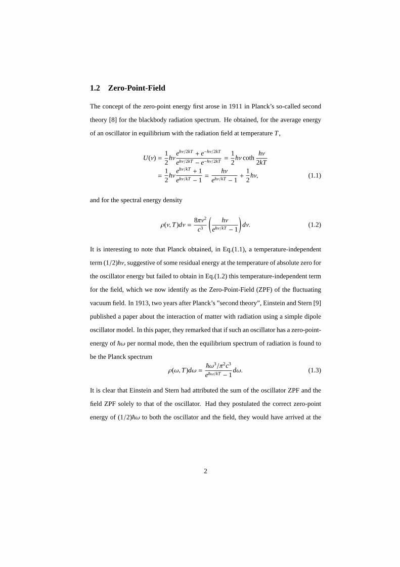
It is interesting to note that Planck obtained, in Eq.(1.1), a temperature-independent

term (1/2)hν, suggestive of some residual energy at the temperature of absolute zero for

the oscillator energy but failed to obtain in Eq.(1.2) this temperature-independent term

for the field, which we now identify as the Zero-Point-Field (ZPF) of the fluctuating

vacuum field. In 1913, two years after Planck’s ”second theory”, Einstein and Stern [9]

published a paper about the interaction of matter with radiation using a simple dipole

oscillator model. In this paper, they remarked that if such an oscillator has a zero-point-

energy of~ω per normal mode, then the equilibrium spectrum of radiation is found to

be the Planck spectrum

ρ(ω,T)dω =~ω3/π2c3

e~ω/kT − 1dω. (1.3)

It is clear that Einstein and Stern had attributed the sum of the oscillator ZPF and the

field ZPF solely to that of the oscillator. Had they postulated the correct zero-point

energy of (1/2)~ω to both the oscillator and the field, they would have arrived at the

2

correct Planck spectrum with the temperature-independent term,

ρ(ν,T)dν =8πν2

c3

(hν

ehν/kT − 1+

hν2

)dν. (1.4)

As this result of Einstein and Stern indicates, there was no concept, at this point, of the

zero-point-field. In 1916, Nernst [10] stated that it is impossible to tell the difference

between matter and field oscillators if they are in thermal contact to attain statistical

equilibrium, and that Planck’s equation (1.1) should therefore hold for both matter and

field oscillators. This statement of Nernst is generally considered as the birth of the

concept of thezero-point-field.

In 1924, Mulliken [11] provides us with a direct evidence of the term (1/2)~ω in the

energy levels of the molecular vibrational spectra of boron monoxide. This is regarded

as the first evidence of the reality of the zero-point energy, and several months after this

Mulliken’s discovery, the quantum formalism had begun to be established, in which the

concept of the zero-point energy appears so naturally.

1.3 Stochastic Electrodynamics

As a result of the pioneering works in the first half of the twentieth century, mentioned

in the previous section, the reality of the zero-point energy and zero-point field had

slowly begun to be realized. This opened up in 1960s a new field of physics called

Stochastic Electrodynamics (SED). SED is, in Boyer’s words [12],

Lorentz’s classical electron theory [13] into which one introduces ran-

dom electromagnetic radiation (classical zero-point radiation) as the bound-

ary condition giving the homogeneous solution of Maxwell’s equations.

The scale of the random radiation is determined with the use of one adjustable param-

eter, which is chosen in terms of Planck’s constanth. This exact form of SED was first

proposed by Marshall [1][2], and further developed by Boyer [14], and it has been suc-

3

cessful in explaining various quantum phenomena within the framework of traditional

classical physics complemented with a classical version of the electromagnetic fluc-

tuations of the vacuum. Some of these successful achievements include: the Casimir

effect [3], the Lamb shift [15], the van der Waals forces [16], atomic stability [17],

Davies-Unruh effect [18], among many others.1

Of particular interest to us in the above is the Davies-Unruh effect, which was dis-

covered in 1975 independently by Davies [20] and Unruh [21] through the study of

Hawking radiation of black holes. This Davies-Unruh effect states that, if accelerated

through vacuum, an observer finds the surrounding vacuum filled with a heat radiation

of temperatureT = ~a/2πck. 2 The meaning of this effect is that an observer under

constant accelerationa finds himself/herself as if he/she were immersedat rest in a

thermal bath of temperatureT = ~a/2πck. This acceleration-dependent Davies-Unruh

effect suggests that there exists some unknown structure of the vacuum which reacts

only against acceleration. If this hidden structure of the vacuum is activated only if

an object is accelerated, then this vacuum might exert a kind of ZPF resistance against

accelerated objects, and this could explain the heretofore unexplored origin of inertia.

Along this line of thoughts, a series of papers was published by Rueda, Haisch, and

Puthoff, and by Rueda and Haisch, in which this ZPF resistive force against acceler-

ation was evaluated using a Planck oscillator model [6], and for a model-independent

case [7]. In both cases, they found that the resistive force is proportional in magnitude

and in the opposite direction to acceleration. In this thesis, the model-independent case

will be studied following Rueda and Haisch’s approach, using aquantum electrody-

namicalformulation.

In the next chapter, a mathematical representation of the zero-point field is intro-

duced, along with the coordinate systems we employ. In Chapter 4, detailed calcula-

tions of the ZPF Poynting vector (momentum density) that an object sweeps through

1For a more detailed history of the developments of SED, refer to de la Pena and Cetto [19], Ch. 4.2Derivation of this Davies-Unruh effect in quantum formulation is given in Appendix F.

4

under its accelerated motion will be shown and the mathematical form of the electro-

magnetic vacuum inertial mass componentmi will be determined. A fully covariant

approach will be taken in Chapter 5 to obtain the same form formi as that obtained in

Chapter 4.

5

2 Zero-Point Radiation

2.1 Zero-Point Field in Classical Random Electrodynamics

The zero-point radiation spectrum has several interesting properties [12]. It is homo-

geneous and isotropic in every inertial frame [17], Lorentz invariant [2, 22], invariant

under an adiabatic compression [10, 23], and invariant under scattering by a dipole

oscillator [17] moving with arbitrary constant velocity.

Theclassicalelectromagnetic zero-point radiation can be written, as a superposi-

tion of plane waves [22],

E(R, t) =

2∑

λ=1

∫d3kε(k, λ)hzp(ω) cos [k · R − ωt − θ(k, λ)] , (2.1)

B(R, t) =

2∑

λ=1

∫d3k

(k× ε

)hzp(ω) cos [k · R − ωt − θ(k, λ)] . (2.2)

Here, the zero-point radiation is expressed in expansion of plane waves and as a sum

over two polarization states ˆε(k, λ), which is a function of the propagation vectork and

the polarization indexλ = 1,2. For each direction of propagation given byk, there

exist two mutually orthogonal polarization states ˆε1 and ε2, where the superscripts 1

and 2 correspond to the polarization indexλ. Hence we have

ε l · εm = δlm, l,m = 1,2, (2.3)

εm · k = 0, m = 1,2. (2.4)

If we consider the third unit vector ˆε3 = k = k/k, wherek is the propagation vector,

then these three vectors form an orthonormal triad,

3∑

λ=1

(ελ

)i

(ελ

)j=

3∑

λ=1

ελi ελj = ε1

i ε1j + ε2

i ε2j + ε3

i ε3j = δi j , (2.5)

6

and also

ε3 = k = ε1 × ε2 (2.6)

and two other relationships of the orthonormal triad can be generated by symmetry:

1→ 2→ 3→ 1.

Note that, in the above, the polarization components ˆελi are to be understood as

scalars. They are the projections of the polarization unit vectors onto thei-axis:

ελi = ελ · xi , xi = x, y, z (2.7)

We also use the same convention with thek unit vector, i.e.,kx = k · x.

The polarization vectors also satisfy the following relationships:

2∑

λ=1

εi ε j = δi j − ki k j (2.8)

2∑

λ=1

εi(k× ε

)j=

∑

k=x,y,z

εi jk kk (2.9)

2∑

λ=1

(k× ε

)i

(k× ε

)j= δi j − ki k j (2.10)

whereεi jk is a Levi-Civita symbol, and the polarization superscriptsλ on the ˆε’s are

omitted for simplicity. Refer to Appendix A for derivations of the relationships above.

In the expressions (2.1) and (2.2), the random phaseθ(k, λ) is introduced, following

Planck [24] and Einstein and Hopf [25], to generate the random, fluctuating nature of

the radiation. Thisθ(k, λ) is a random variable distributed uniformly in the interval

(0,2π) and independently for each wave vectork and the polarization indexλ. Also the

spectral functionhzp(ω) is introduced to set the magnitude of the zero-point radiation,

which is found in terms of the Planck’s constanth as [22]

h2zp(ω) =

~ω

2π2. (2.11)

7

Plack’s constant enters the theory at this point only as a scale factor to attain correspon-

dence between zero temperature random radiation of (classical) stochastic electrody-

namics and the vacuum zero point field of quantum electrodynamics. A derivation of

this spectral function is also given in Appendix B and it is found that this value for the

spectral function is slightly different in the quantum electrodynamical case.

2.2 Zero-Point-Field in Quantum Electrodynamics

In this thesis, a quantum approach is used instead of the classical stochastic approach,

to evaluate the vacuum expectation values of the zero-point field. The QED formulation

of the zero point electric and magnetic fields are also expressed by the expansion in

plane waves as [26, 27]

E(r , t) =

2∑

λ=1

∫d3kε(k , λ)Hzp(ω)

[α (k, λ) exp(−iωt + ik · r ) + α† (k, λ) exp(iωt − ik · r )

],

(2.12)

B(r , t) =

2∑

λ=1

∫d3k(k× ε)Hzp(ω)

[α (k, λ) exp(−iωt + ik · r ) + α† (k, λ) exp(iωt − ik · r )

].

(2.13)

Here the polarization unit vectors ˆε (k, λ) (λ = 1,2) and the wave vectork are the

same as those in the random fields (2.1) and (2.2). The cosine functions in the random

electrodynamics formulation are now replaced with the exponential functions and the

quantum operatorsα(k, λ) andα†(k, λ). These quantum operators are annihilation and

creation operators on the Hilbert space and satisfy the commutation rules

[α (k, λ) , α

(k′, λ′

)]=

[α† (k, λ) , α†

(k′, λ′

)]= 0 (2.14)

[α (k, λ) , α†

(k′, λ′

)]= δλ,λ′δ

3(k − k′) (2.15)

8

and have the expectation values,

⟨0∣∣∣α (k, λ)α

(k′, λ′

)∣∣∣ 0⟩

=⟨0∣∣∣α† (k, λ)α†

(k′, λ′

)∣∣∣ 0⟩

= 0 (2.16)⟨0∣∣∣α (k, λ)α†

(k′, λ′

)∣∣∣ 0⟩

= δλ,λ′δ3(k − k′) (2.17)

⟨0∣∣∣α† (k, λ)α

(k′, λ′

)∣∣∣ 0⟩

= 0 (2.18)

The overline onE and B in Eq.(2.12) and (2.13) indicates that these fields are now

given as operators.

Also the spectral function, introduced to set the scale of the radiations, is expessed

asHzp(ω) using an uppercase H to distinguish this from the classicalhzp(ω). It is found

in Appendix B that the value of thisHzp(ω) is

H2zp(ω) =

~ω

4π2, (2.19)

which is not the same as the classical caseh2zp(ω) = ~ω/2π2.

9

3 Correspondence between Random and Quantum Zero-

Point Field

In Rueda and Haisch’s classical approach, averaged field fluctuations were evaluated

using the two-point correlation functions. In the quantum approach used in the present

research, however, the expectation values of the vacuum field will be evaluated using

the creation and annihilation operators. Although these two approaches are similar in

some respects, there also exist several major differences, which was first pointed out

by Boyer [26].

In this chapter, following Boyer’s analysis, a brief comparison is presented between

random electrodynamics and quantum electrodynamics. The connection between the

two-point correlation functions in free-field quantum electrodynamics and in random

electrodynamics is examined, and it is found that they are in general not equal to each

other because of the dependence on the order of the quantum operators. However, if

all the products of quantum operators are symmetrized by taking all the permutations

of the operator order, then the two theories yield identical results for the correlation

functions.

3.1 Two-Point Correlation Function

The electromagnetic field fluctuations may be characterized by the field correlation

functions at two different points in space and in time. Therefore, in order to evaluate

the correlation in random electrodynamics, averaging over the random phases is taken,

10

and we obtain

⟨Ei(r1, t1)E j(r2, t2)

⟩=

2∑

λ1=1

2∑

λ2=1

∫d3k1

∫d3k2ε1 (k1, λ1) ε2 (k2, λ2) hzp (k1, λ1) hzp (k2, λ2)

× 〈cos[k1 · r1 − ω1t1 + θ(k1, λ1)] cos[k2 · r2 − ω2t2 + θ(k2, λ2)]〉

=

2∑

λ=1

∫d3kεi (k , λ) ε j (k , λ) h2

zp (k , λ)12

cos[k · (r1 − r2) − ω(t1 − t2)]

=

∫d3k

(δi j − ki k j

) ~ω4π2

cos[k · (r1 − r2) − ω(t1 − t2)], (3.1)

where the averages

〈cosθ(k1, λ1) cosθ(k2, λ2)〉 = 〈sinθ(k1, λ1) sinθ(k2, λ2)〉

=12δλ1λ2δ

3 (k1 − k2) (3.2)

and

〈cosθ(k1, λ1) sinθ(k2, λ2)〉 = 0 (3.3)

were used in the second equality. Also the polarization relation (2.8), i.e.,

2∑

λ=1

εi ε j = δi j − ki k j (3.4)

was used in the last equality.

It can be easily shown by similar calculations that we also obtain

⟨Bi(r1, t1)B j(r2, t2)

⟩=

⟨Ei(r1, t1)E j(r2, t2)

⟩(3.5)

and

⟨Ei(r1, t1)B j(r2, t2)

⟩=

∫d3kεikl kl

~ω

4π2cos[k · (r1 − r2) − ω(t1 − t2)]. (3.6)

11

In quantum electrodynamics, analogous expressions can be obtained as well with

the use of the expectation values (2.16)-(2.18), and the polarization equations (2.8)-

(2.10). For example, the vacuum expectation value of two electric zero-point field at

two different spaceR1 andR2 and two different timet1 andt2 would be,

⟨0∣∣∣Ei(r1, t1)E j(r2, t2)

∣∣∣ 0⟩

=

2∑

λ1=1

2∑

λ2=1

∫d3k1

∫d3k2ε1 (k1, λ1) ε2 (k2, λ2)

× Hzp (k1, λ1) Hzp(k2, λ2)⟨0∣∣∣∣[α(k1, λ1)eiΘ1 + α†(k1, λ1)e−iΘ1

]

×[α(k2, λ2)eiΘ2 + α†(k2, λ2)e−iΘ2

]∣∣∣∣ 0⟩, (3.7)

where the form of the ZPF is given by Eq.(2.12), and

Θ1 = k1 · r1 − ω1t1,

Θ2 = k2 · r2 − ω2t2. (3.8)

Note that we are not allowed to change the order of any operators in the quantum

case. Hence the expression above has four terms and each of them has to be evaluated

independently. However, we can easily see from the relations Eq.(2.16)-Eq.(2.18),

that only one term proportional toα(k1, λ1)α†(k2, λ2) is non-vanishing. Therefore, the

above equation simplifies to

⟨0∣∣∣Ei(r1, t1)E j(r2, t2)

∣∣∣ 0⟩

=

2∑

λ1=1

2∑

λ2=1

∫d3k1

∫d3k2ε1 (k1, λ1) ε2 (k2, λ2)

× Hzp (k1, λ1) Hzp (k2, λ2)⟨0∣∣∣α(k1, λ1)α†(k2, λ2)

∣∣∣ 0⟩

× exp(−iω1t1 + ik1 · r1) exp(iω2t2 − ik2 · r2), (3.9)

which, with the help of Eq.(2.17), yields the desired result

⟨0∣∣∣Ei(r1, t1)E j(r2, t2)

∣∣∣ 0⟩

=

∫d3k

(δi j − ki k j

) ~ω4π2

exp[ik ·(r1−r2)− iω(t1−t2)] (3.10)

12

In a similar manner, the following two relationships can also be found:

⟨0∣∣∣Bi(r1, t1)B j(r2, t2)

∣∣∣ 0⟩

=⟨0∣∣∣Ei(r1, t1)E j(r2, t2)

∣∣∣ 0⟩

(3.11)⟨0∣∣∣Ei(r1, t1)B j(r2, t2)

∣∣∣ 0⟩

=

∫d3k

(εi jl kl

) ~ω4π2

exp[ik · (r1 − r2) − iω(t1 − t2)] (3.12)

3.2 Discrepancies between SED and QED

From the results in the previous section, we see that the expressions for the average

do not agree with each other. However, these discrepancies can easily be explained in

terms of the operator order. In random electrodynamics, the order of the fields has no

significance upon the averaging, i.e.,

⟨Ei(r1, t1)E j(r2, t2)

⟩=

⟨E j(r1, t1)Ei(r2, t2)

⟩. (3.13)

On the other hand, in quantum electrodynamics, the operators do not commute and the

order does matter,

⟨0∣∣∣Ei(r1, t1)E j(r2, t2)

∣∣∣ 0⟩,

⟨0∣∣∣E j(r1, t1)Ei(r2, t2)

∣∣∣ 0⟩

(3.14)

In quantum mechanics, physical observables are expressed in terms ofHermitian

operators. It can be shown that if we symmetrize these operators by taking the every

possible permutations and then average the sum, there exists exact agreement between

the correlations in random and quantum electrodynamics. To show this correspon-

dence, we first notice that the correlation function (3.1) and the vacuum expectation

value (3.10) in quantum electrodynamics have the same form and the only difference

is that the cosine function is replaced by the exponentials in QED.

13

Let us consider the Eq(3.10) and the different order of it in the electric fields,

⟨0∣∣∣E j(r2, t2)Ei(r1, t1)

∣∣∣ 0⟩

=

∫d3k

(δi j − ki k j

) ~ω4π2

exp[ik · (r2 − r1) − iω(t2 − t1)]

=

∫d3k

(δi j − ki k j

) ~ω4π2

exp[−ik · (r1 − r2) − iω(t1 − t2)].

(3.15)

Note that Eq(3.10) and Eq(3.15) are slightly different in that the exponent has a negative

sign in Eq(3.15). Now we add Eq(3.10) and the equation above to obtain

⟨0∣∣∣Ei(r1, t1)E j(r2, t2)

∣∣∣ 0⟩

+⟨0∣∣∣E j(r2, t2)Ei(r1, t1)

∣∣∣ 0⟩

=

∫d3k

(δi j − ki k j

) ~ω4π2

exp[ik · (r1 − r2) − iω(t1 − t2)]

+ exp[−ik · (r1 − r2) − iω(t1 − t2)]

=

∫d3k

(δi j − ki k j

) ~ω4π2

2 cos[k · (r1 − r2) − iω(t1 − t2)]

(3.16)

Notice the presence of the extra factor of two in the last equality, which does not exist

in the SED case. This result produces the following relationship,

12

⟨0∣∣∣Ei(r1, t1)E j(r2, t2) + E j(r2, t2)Ei(r1, t1)

∣∣∣ 0⟩

=

∫d3k

(δi j − ki k j

) ~ω4π2

cos[k · (r1 − r2) − iω(t1 − t2)]

and the desired correspondence,

⟨Ei(r1, t1)E j(r2, t2)

⟩=

12

⟨0∣∣∣Ei(r1, t1)E j(r2, t2) + E j(r2, t2)Ei(r1, t1)

∣∣∣ 0⟩

=12

[⟨0∣∣∣Ei(r1, t1)E j(r2, t2)

∣∣∣ 0⟩

+⟨0∣∣∣E j(r2, t2)Ei(r1, t1)

∣∣∣ 0⟩]

(3.17)

is obtained. It can also be easily shown that this agreement between the correlation

14

function in random electrodynamics and the vacuum expectation value in quantum

electrodynamics also holds for the other two-point functions (3.11) and (3.12) as well.

These discrepancies between SED and QED, stemming from the non-commutivity of

the quantum operators keep arising in all orders. However, regardless of the order,

if we construct the symmetrized operators, the correspondence between two theories

would be achieved [26].

3.3 Heisenberg Picture and Schroedinger Picture

In a formulation of a system in quantum mechanics, time evolution can be treated in

two different manners: we can either absorb the time evolution in the state vector|Ψ(t)〉and treat the operator as constant in time, or let the state vector to be time constant and

treat the operator as a time dependent quantity,A = A(t). The former is called the

Schroedinger pictureand the latter theHeisenberg picture. In our research, we are

obviously adopting the Heisenberg picture, for our state vector|0〉 is always fixed in

time and the time dependence is absorbed in the operators.

It is known that the difference between these two formulations is just the way in

which time evolution is handled and they are in most cases equivalent otherwise.3

The results and predictions of quantum mechanics are not affected by the choice of the

formulation. Therefore, the correspondence between the SED and QED also remains

unaffected by our choice of the Heisenberg picture.

Regarding the Heisenberg picture and its agreement with random electrodynamics,

Milonni4 remarks the following:

The equations of motion are formally the same in the two theories. The

final step in the derivation involves a term bilinear in the zero-point elec-

tric field. In the quantum electrodynamics case we require an expectation

3A possibility of discrepancy between the Schrodinger and the Heisenberg picture has been pointed outby A. J. Faria et al.[28]. They claim that the effects of the zero-point field may be counted twice in theSchrodinger treatment of the oscillator.

4P.W. Milonni, Physics Reports25, No.1 (1976) pp. 1-81.

15

value of this term over the vacuum field state. In random electrodynamics

we require an average of formally the same term over the random phases of

the zero-point field. The two types of ensemble average yield the same an-

swer, and therefore the same result for the van der Waals interaction. From

this view point, we might even contend that the principal merit in Boyer’s

derivation is the treatment of the problem in the Heisenberg picture, with

a consequent ease of physical interpretation.

Although this comment was made on the derivation of the van der Waals forces, our

research involves essentially the same procedure: the expectation values of the electro-

magnetic fields over the vacuum state in quantum electrodynamics, and the averages

of the fields over the random phases of the zero-point field in random electrodynamics.

The strong similarity between the Heisenberg picture treatment and random electrody-

namics is equally valid in our research as well.

16

4 Evaluation of the ZPF Poynting Vector

4.1 Overview

In this chapter, the Poynting vectorSzp∗ of the zero-point field that an object sweeps

through under its constantly accelerated motion is evaluated in the laboratory inertial

frame. The object has a proper volumeV0 in its own rest frame and is accelerated

along the positivex-direction, that is,a = ax. Since the Poynting vector is physically a

momentum flux, we can also find out its momentum densitygzp∗ by dividing the Poynt-

ing vector byc2, i.e.,gzp∗ = Szp

∗ /c2. Since the ZPF spectrum is Lorentz-invariant, this

momentum density is a time-independent constant under constant velocity. However,

under the constantaccelerationwe consider in this research, this momentum density

will become a function of time. Therefore, once we find out this momentum density,

the force that the ZPF exerts upon the accelerated object can be determined as well by

taking the time derivative of the momentum. It will be shown that this ZPF resistive

force is directly proportional to the acceleration and directed against the acceleration.

Consider an inertial observer at rest in the laboratory frameI∗. This observer will

find that the ZPF is isotropically distributed around himself, and that the ZPF Poynt-

ing vectorSzp∗ is zero, for there is no flux of ZPF in this situation. Now consider an

object moving with constant velocity along thex-axis,v = vxx. Since the ZPF spec-

trum is Lorentz-invariant, both the stationaryI∗-observer and the observer comoving

with the object will see the ZPF isotropically distributed around themselves. How-

ever, theI∗-observer will not find the ZPF of the other observer comoving with the

object isotropically distributed around himself, since the Doppler effects shift the wave

vectork depending on the velocity of the object. This of course is true for the ZPF

of the I∗-observer as seen from the moving observer as well. In this situation where

the object is moving with constant velocity, theI∗-observer will find that the object

carries a momentump∗ = γm0v, and that both the ZPF Poynting vectorSzp∗ and its

17

corresponding momentum densitygzp∗ = Szp

∗ /c2 are non-zero, which remain constant

independent of time. Moreover, if the object is under hyperbolic motion (constantly

accelerated motion), then the ZPF spectrum is not time independent any more and the

ZPF momentum seen from theI∗-observer view point becomes a function of time (Eq.

(4.54)), and consequently the time derivative of the momentum becomes nonvanishing

(Eq. (4.55)).

The discussions above can also be explained in the same manner using the concept

of thek-sphere.5 In evaluating the ZPF Poynting vector, we perform integrations ink-

space up to the cut-off radiuskc = ωc/c centered at the observation point, with the cut-

off frequencyωc associated with the ZPF spectral distribution. Every inertial observer

has his ownk-sphere spherically symmetrically distributed around himself. In the case

of the constant velocity discussed above, the observer comoving with the object will

find that the object is at the center of his ownk-sphere, and the object appears to carry

no mechanical or ZPF momenta whatsoever. However, this situation would become

quite different from the point of view of theI∗-observer, since the object is not located

at the center of his ownk-sphere. From theI∗-observer’s view, the object appears to

carry both mechanical momentump∗ = γm0v and the ZPF momentum densitygzp∗ ,

which are both constants independent of time. As soon as this object get accelerated

by an external agent, both the ZPF momentum density and the corresponding ZPF

momentumpzp∗ = V∗g

zp∗ as seen from theI∗-observer become acceleration dependent

functions of time, which, later in this chapter, we find to be

gzp∗ (τ) =

Szp∗ (τ)c2

= −x1

4πc8π3

sinh

(2aτc

) ∫~ω3

2π2c3dω, (4.1)

and

pzp∗ (τ) = V∗g

zp∗ =

V0

γτgzp∗ (τ) = −x

4V0

3cβτγτ

∫~ω3

2π2c3dω. (4.2)

5For more detailed explanations of thek-sphere, see A. Rueda and B. Haisch, Found. Phys. 28, 1057,1998, especially Appendix C.

18

Since this ZPF momentum density is a function of time, we can find the time deriva-

tives of this functionf zp∗ = dpzp

∗ /dt∗, and we interpret that this is the force that the ZPF

exerts upon the accelerated objects.

4.2 Constant Proper Acceleration (Hyperbolic Motion)

As a basis of our analysis, we employ the following system of reference frames [18, 7]:

an inertial laboratory frameI∗, the accelerated frameS in which the object is placed at

rest at the point (c2/a,0,0), and a set of instantaneous inertial framesIτ defined at each

of the object’s proper timeτ. The accelerated frameS comoving with the object is set

to coincide with the lab frameI∗ whent∗ = τ = 0.

The object is at rest at the point (c2/a,0,0) in the accelerated frameS, and the ac-

celeration is in the positivex-direction. This acceleration of the (c2/a,0,0) point inS

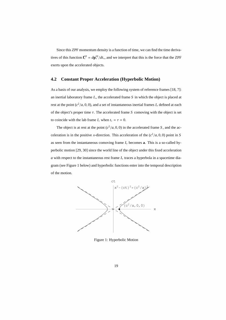
as seen from the instantaneous comoving frameIτ becomesa. This is a so-called hy-

perbolic motion [29, 30] since the world line of the object under this fixed acceleration

a with respect to the instantaneous rest frameIτ traces a hyperbola in a spacetime dia-

gram (see Figure 1 below) and hyperbolic functions enter into the temporal description

of the motion.

x

ct

Hc2a,0,0L

x2-HctL2=Hc2aL2

Figure 1: Hyperbolic Motion

19

In this system of hyperbolic motion, the object’s position and time inI∗ are ex-

pressed in terms of the proper timeτ as

t∗ =ca

sinh(aτ

c

), (4.3)

x∗ = R∗(τ) · x =c2

acosh

(aτc

), (4.4)

y∗ = 0, (4.5)

z∗ = 0, (4.6)

whereR∗ is the object’s coordinates as seen from theI∗ lab reference frame, which is

chosen to be (c2/a,0,0) in bothI∗ andS frames whent = τ = 0. Note thatx2∗ − (ct∗)2 =

c4/a2, which is an equation for a hyperbola.

Similarly, the magnitude of the velocityu∗(τ) with respect toI∗ is given by

βτ =u∗(τ)

c=

1c

dx∗dt∗

=1c

dx∗/dτdt∗/dτ

= tanh(aτ

c

), (4.7)

where we introduced the normalized velocityβτ. We also use the correspondingγ-

factor, namely,

γτ =1√

1− β2τ

=1

sech(aτ/c)= cosh

(aτc

). (4.8)

Both (4.7) and (4.8) are hyperbolic functions.

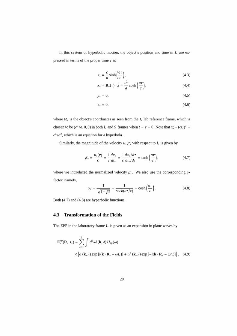
4.3 Transformation of the Fields

The ZPF in the laboratory frameI∗ is given as an expansion in plane waves by

Ezp∗ (R∗, t∗) =

2∑

λ=1

∫d3kε (k, λ) Hzp(ω)

×α (k, λ) exp [i(k · R∗ − ωt∗)] + α† (k, λ) exp [−i(k · R∗ − ωt∗)]

, (4.9)

20

and

Bzp∗ (R∗, t∗) =

2∑

λ=1

∫d3k

(k× ε

)Hzp(ω)

×α (k, λ) exp [i(k · R∗ − ωt∗)] + α† (k, λ) exp [−i(k · R∗ − ωt∗)]

, (4.10)

whereR∗ andt∗ are the space and time coordinates of the observation point inI∗. The

polarization unit vectors ˆε (k, λ) (λ = 1,2) are orthogonal to each other and to the wave

vectork, and the functionHzp(ω) is defined in such a way that it corresponds to the

electromagnetic energy per normal mode at frequencyω, that is,

H2zp(ω) =

~ω

4π2. (4.11)

Since thisI∗ lab frame is the ultimate reference frame where all the physical quan-

tities of the accelerating object inIτ frame is to be evaluated, in order to obtain the

ZPF that the object is subjected to in the accelerated frame, we transform these fields

from the inertial frameI∗ to the correspondingIτ frame using the standard Lorentz-

transformation of the fields, namely,

E′1 = E1 B′1 = B1

E′2 = γ(E2 − βB3) B′2 = γ(B2 + βE3)

E′3 = γ(E3 + βB2) B′3 = γ(B3 − βE2)

(4.12)

21

and obtain

Ezpτ (0, τ) =

2∑

λ=1

∫d3k

xεx + yγτ[εy − βτ(k× ε)z] + zγτ[εz + βτ(k× ε)y]

Hzp(ω)

×α (k, λ) exp [i(k · R∗ − ωt∗)] + α† (k, λ) exp [−i(k · R∗ − ωt∗)]

, (4.13)

Bzpτ (0, τ) =

2∑

λ=1

∫d3k

x(k× ε)x + yγτ[(k× ε)y + βτεz] + zγτ[(k× ε)z − βτεy]

× Hzp(ω)α (k, λ) exp [i(k · R∗ − ωt∗)] + α† (k, λ) exp [−i(k · R∗ − ωt∗)]

.

(4.14)

The arguments of the fields are taken as zero but it actually means theIτ spatial

point (c2/a,0,0).

We assume that the object is subject to a constant acceleration, i.e., a hyperbolic

motion. Then as seen before (4.3-4.8), the velocity in the comoving frameIτ with

respect toI∗ and the space and time coordinates of the object inIτ are given by

βτ = u∗(τ)/c = tanh(aτ/c), (4.15)

γτ =1√

1− β2τ

=1

sech(aτ/c)= cosh(aτ/c), (4.16)

R∗(τ) · x = (c2/a) cosh(aτ/c), (4.17)

t∗ = (c/a) sinh(aτ/c). (4.18)

22

Putting these into the above expressions for the fields (4.13) and (4.14), we obtain,

Ezpτ (0, τ) =

2∑

λ=1

∫d3k

xεx + ycosh

(aτc

) [εy − tanh

(aτc

)(k× ε)z

]

+ zcosh(aτ

c

) [εz + tanh

(aτc

)(k× ε)y

]Hzp(ω)

×α (k, λ) exp

[i

(kx

c2

acosh

(aτc

)− ωc

asinh

(aτc

))]

+ α† (k, λ) exp

[−i

(kx

c2

acosh

(aτc

)− ωc

asinh

(aτc

))](4.19)

Bzpτ (0, τ) =

2∑

λ=1

∫d3k

x(k× ε)x + ycosh

(aτc

) [(k× ε)y + tanh

(aτc

)εz

]

+ zcosh(aτ

c

) [(k× ε)z − tanh

(aτc

)εy

]Hzp(ω)

×α (k, λ) exp

[i

(kx

c2

acosh

(aτc

)− ωc

asinh

(aτc

))]

+ α† (k, λ) exp

[−i

(kx

c2

acosh

(aτc

)− ωc

asinh

(aτc

))](4.20)

where the quantum operatorsα (k, λ) andα† (k, λ) are the annihilation and creation

operators on the Hilbert space respectively, which satisfy the commutation rules

[α (k, λ) , α

(k′, λ′

)]=

[α† (k, λ) , α†

(k′, λ′

)]= 0 (4.21)

[α (k, λ) , α†

(k′, λ′

)]= δλ,λ′δ

3(k − k′) (4.22)

and have the expectation values,

⟨0∣∣∣α (k, λ)α

(k′, λ′

)∣∣∣ 0⟩

=⟨0∣∣∣α† (k, λ)α†

(k′, λ′

)∣∣∣ 0⟩

= 0 (4.23)⟨0∣∣∣α (k, λ)α†

(k′, λ′

)∣∣∣ 0⟩

= δλ,λ′δ3(k − k′) (4.24)

⟨0∣∣∣α† (k, λ)α

(k′, λ′

)∣∣∣ 0⟩

= 0 (4.25)

Notice here that the order of the quantum operator affects the result as mentioned in

the earlier chapter. This problem does not arise in the classical random variable cases.

23

The expressions for the fields above, (4.19) and (4.20) are the ZPF as instanta-

neously viewed from the object fixed to the point (c2/a,0,0) of S that is performing

the hyperbolic motion.

4.4 Evaluation of the Poynting vector components

We now evaluate the ZPF Poynting vector corresponding to the radiation being swept

through by the accelerated object as seen from the observer at rest at (c2/a,0,0) of I∗,

using the expression for the fields obtained in the previous section, that is,

Ezpτ (0, τ) =

2∑

λ=1

∫d3k

xεx + ycosh

(aτc

) [εy − tanh

(aτc

)(k× ε)z

]

+ zcosh(aτ

c

) [εz + tanh

(aτc

)(k× ε)y

]Hzp(ω)

×α (k, λ) exp

[i

(kx

c2

acosh

(aτc

)− ωc

asinh

(aτc

))]

+ α† (k, λ) exp

[−i

(kx

c2

acosh

(aτc

)− ωc

asinh

(aτc

))](4.26)

Bzpτ (0, τ) =

2∑

λ=1

∫d3k

x(k× ε)x + ycosh

(aτc

) [(k× ε)y + tanh

(aτc

)εz

]

+ zcosh(aτ

c

) [(k× ε)z − tanh

(aτc

)εy

]Hzp(ω)

×α (k, λ) exp

[i

(kx

c2

acosh

(aτc

)− ωc

asinh

(aτc

))]

+ α† (k, λ) exp

[−i

(kx

c2

acosh

(aτc

)− ωc

asinh

(aτc

))](4.27)

In all of the evaluations of the vacuum expectation values for the electric and mag-

netic components of the ZPF,⟨0∣∣∣Ei Bj

∣∣∣ 0⟩, i, j = x, y, z, to follow in this section, we

need to evaluate the following quantity,

⟨0∣∣∣∣α (k, λ) eiΘ + α† (k, λ) e−iΘ

×

α(k′, λ′

)eiΘ′ + α†

(k′, λ′

)e−iΘ′

∣∣∣∣ 0⟩

(4.28)

24

where

Θ = kxc2

acosh

(aτc

)− ωc

asinh

(aτc

)(4.29)

and

Θ′ = k′xc2

acosh

(aτc

)− ω′ c

asinh

(aτc

)(4.30)

In order to evaluate this quantity, we make use of the expectation value relation-

ships for the quantum creation and annihilation operators (4.23)-(4.25), and it is found

that only terms proportional to⟨0∣∣∣α (k, λ)α† (k′, λ′)

∣∣∣ 0⟩

remain and all the other terms

vanish. Therefore, we have

⟨0∣∣∣Ei(k, λ)Bj(k′, λ′)

∣∣∣ 0⟩∝ eiΘe−iΘ′ ×

⟨0∣∣∣α (k, λ)α†

(k′, λ′

)∣∣∣ 0⟩

∝ δλ,λ′δ3(k − k′)eiΘ(k)e−iΘ′(k′) (4.31)

where

Θ(k) = kxc2

acosh

(aτc

)− ωc

asinh

(aτc

),

Θ′(k′) = k′xc2

acosh

(aτc

)− ω′ c

asinh

(aτc

).

As explained in the previous chapter, in order to assure the correspondence between

the random electrodynamics and the quantum electrodynamics results, it is required to

construct the symmetrized operators in the QED case by taking every possible permu-

tations of the field operators, that is,

⟨Ei(r1, t1)B j(r2, t2)

⟩=

12

⟨0∣∣∣Ei(r1, t1)B j(r2, t2) + B j(r2, t2)Ei(r1, t1)

∣∣∣ 0⟩. (4.32)

However, due to the symmetrical form of the zero-point field with respect to the quan-

25

tum operators, i.e.,

Ei(k, λ) ∝α (k, λ) eiΘ + α† (k, λ) e−iΘ

, (4.33)

B j(k′, λ′) ∝α(k′, λ′

)eiΘ′ + α†

(k′, λ′

)e−iΘ′

, (4.34)

and the expectation value relationship (4.23)-(4.25), it is clear that

⟨0∣∣∣Ei(k, λ)B j(k′, λ′)

∣∣∣ 0⟩

=⟨0∣∣∣B j(k′, λ′)Ei(k, λ)

∣∣∣ 0⟩, (4.35)

which gives us a simple relation between SED and QED,

⟨Ei(k, λ)B j(k′, λ′)

⟩=

⟨0∣∣∣Ei(k, λ)B j(k′, λ′)

∣∣∣ 0⟩, (4.36)

which always holds in the cases of our interest.

Now, we proceed with the explicit evaluations of the ZPF expectation values. Let

Szp denote the ZPF Poynting vector. ThenSzp∗ , the ZPF Poynting vector that enters the

body of the accelerating object in the instantaneous comoving frameIτ, evaluated from

the laboratory inertial frameI∗, is given by

Szp∗ =

c4π

⟨0∣∣∣Ezp

τ × Bzpτ

∣∣∣ 0⟩∗

=c

4π

x⟨0∣∣∣EyBz − EzBy

∣∣∣ 0⟩

+ y 〈0 |EzBx − ExBz|0〉

+ z⟨0∣∣∣ExBy − EyBx

∣∣∣ 0⟩. (4.37)

It turns out that only thex-component of the ZPF Poynting vector is non-vanishing

and the other components are zero. The detailed calculations of each component of this

Poynting vector is shown in Appendix C, and only a brief summary of this evaluation

will be shown below.

In order to evaluate the vacuum expectation value for a component of the ZPF

26

Poynting vector, e.g.,〈0 |ExBx|0〉, thex-component of the zero-point electric field op-

erators (4.26), that is,

Ezpτx(0, τ) =

2∑

λ=1

∫d3k xεxHzp(ω)

×α (k, λ) exp

[i

(kx

c2

acosh

(aτc

)− ωc

asinh

(aτc

))]

+ α† (k, λ) exp

[−i

(kx

c2

acosh

(aτc

)− ωc

asinh

(aτc

))](4.38)

and they-component of the zero-point magnetic field operators (4.27), i.e.,

Bzpτx(0, τ) =

2∑

λ=1

∫d3k

x(k× ε)xHzp(ω)

×α (k, λ) exp

[i

(kx

c2

acosh

(aτc

)− ωc

asinh

(aτc

))]

+ α† (k, λ) exp

[−i

(kx

c2

acosh

(aτc

)− ωc

asinh

(aτc

))](4.39)

are multiplied together and the following expression is obtained:

〈0 |ExBx|0〉 =

2∑

λ=1

2∑

λ′=1

∫d3k

∫d3k′εx(k

′ × ε′)xH2zp(ω)

⟨0∣∣∣∣α (k, λ) exp[iΘ] + α† (k, λ) exp[−iΘ]

×α(k′, λ′

)exp[iΘ′] + α†

(k′, λ′

)exp[−iΘ′]

∣∣∣∣ 0⟩, (4.40)

where

Θ = kxc2

acosh

(aτc

)− ωc

asinh

(aτc

)(4.41)

and

Θ′ = k′xc2

acosh

(aτc

)− ω′ c

asinh

(aτc

). (4.42)

The above expression has four terms, but only the term that is proportional to⟨0∣∣∣α (k, λ)α† (k′, λ′)

∣∣∣ 0⟩

remains as in (4.24), and the above expression is simplified

27

to

〈0 |ExBx|0〉 =

2∑

λ=1

2∑

λ′=1

∫d3k

∫d3k′εx(k

′ × ε′)xH2zp(ω)

×⟨0∣∣∣α (k, λ)α†

(k′, λ′

)∣∣∣ 0⟩

exp [iΘ(k)] exp[−iΘ′(k′)

], (4.43)

with the use of the expectation values

⟨0∣∣∣α (k, λ)α

(k′, λ′

)∣∣∣ 0⟩

=⟨0∣∣∣α† (k, λ)α†

(k′, λ′

)∣∣∣ 0⟩

= 0 (4.44)⟨0∣∣∣α (k, λ)α†

(k′, λ′

)∣∣∣ 0⟩

= δλ,λ′δ3 (

k − k′)

(4.45)⟨0∣∣∣α† (k, λ)α

(k′, λ′

)∣∣∣ 0⟩

= 0. (4.46)

Since the term in the second line in (4.43) isδλ,λ′δ3 (k − k′) exp[iΘ(k)] exp [−iΘ′(k′)],

Eq.(4.43) becomes

〈0 |ExBx|0〉 =

2∑

λ=1

2∑

λ′=1

∫d3k

∫d3k′εx(k

′ × ε′)xH2zp(ω)

×δλ,λ′δ3 (k − k′

)exp[iΘ(k)] exp

[−iΘ′(k′)], (4.47)

which, after one integration over thek-sphere, reduces to

〈0 |ExBx|0〉 =

2∑

λ=1

∫d3kεx(k× ε)xH

2zp(ω). (4.48)

With a use of the polarization formula (A.7) derived in Appendix A, we find that

2∑

λ=1

εx(k× ε)x =∑

k=x,y,z

εiik kk = 0, (4.49)

and after substituting this result into the equation above, it is concluded that〈0 |ExBx|0〉 =

0.

The remaining eight components of the Poynting vector can also be evaluated in a

28

similar manner (for detailed calculations, refer to Appendix C), and it is found that only

the following two terms remain non-vanishing, each of which has the same magnitude

and in the opposite direction to each other:

⟨0∣∣∣EyBz

∣∣∣ 0⟩

= −4π3

sinh

(2aτc

) ∫~ω3

2π2c3dω, (4.50)

and⟨0∣∣∣EzBy

∣∣∣ 0⟩

=4π3

sinh

(2aτc

) ∫~ω3

2π2c3dω. (4.51)

With the results above, the Poynting vectorSzp∗ (4.37) becomes

Szp∗ = x

c4π

⟨0∣∣∣Ezp

τ (0, τ) × Bzpτ (0, τ)

∣∣∣ 0⟩

x

= −xc

4π8π3

sinh

(2aτc

) ∫~ω3

2π2c3dω. (4.52)

This represents the energy flux, i.e., the ZPF energy that enter the uniformly acceler-

ating object’s body per unit area per unit time as seen from the observer at rest in the

inertial laboratory frameI∗.

4.5 Derivation of the Inertial Mass

In the previous section and in Appendix C, all of the Poynting vector components⟨0∣∣∣Ei Bj

∣∣∣ 0⟩

wherei, j = x, y, zwere evaluated and it turned out that all the components

vanish except two, and the ZPF Poynting vector turns out to have onlyx-components

(4.52).

We can also find the momentum density, i.e., field momentum per unit volume that

the field possesses at the object position, (c2,0,0) in the accelerated frameS, at object

proper timeτ and estimated from the view point ofI∗. For this purpose, we divide

29

Szp∗ (τ) by c2, and obtain

gzp∗ (τ) =

Szp∗ (τ)c2

= −x1

4πc8π3

sinh

(2aτc

) ∫~ω3

2π2c3dω. (4.53)

The total amount of momentum due to the ZPF radiation inside the volume of the

object and evaluated in the laboratoryI∗ frame is simplygzp∗ multiplied by the volume

V∗, which gives

pzp∗ (τ) = V∗g

zp∗ =

V0

γτgzp∗ (τ) = −x

4V0

3cβτγτ

∫~ω3

2π2c3dω (4.54)

where equations (4.7) and (4.8) and the relation sinh 2x = 2 sinhxcoshx were used.

At proper timeτ = 0, the time in the laboratory inertial framet∗ = γττ is of course

also zero, and the Rindler frameS and the laboratory frameI∗ exactly coincide mo-

mentarily, and the object location, (c2/a,0,0) of S, matches the observer’s position in

his laboratory frameI∗ as well. If the object is moving at a constant speed, theI∗-

observer will find the ZPF momentum of the object to be timeindependentconstant of

motion. However, under the hyperbolic motion that we consider in this research, the

object appears from the view point of theI∗-observer to be carrying a timedependent

ZPF momentumpzp∗ (4.54), due to the acceleration of the object. Since this ZPF mo-

mentum of the object as observed in theI∗ frame varies with time, we can evaluate the

time rate of change of this momentum,

f zp∗ =

dpzp∗

dt∗=

1γτ

dpzp∗

dτ

∣∣∣∣∣∣τ=0

= −x

[4V0

3c2

∫~ω3

2π2c3dω

]a (4.55)

This f zp∗ is the force exerted on the object by the ZPF radiation as seen in the labo-

ratory inertial frameI∗ at t∗ = 0. We note here that this force is directed in the opposite

direction to the object’s motion, and its magnitude is proportional to the object’s accel-

eration.

30

Moreover, the scalar quantity,

mi =

[V0

c2

∫η(ω)

~ω3

2π2c3dω

](4.56)

has a dimension of mass and we interpret this as an expression of inertial mass arising

from the interaction of the object with the ZPF. The numerical factor of 4/3 has been

neglected here since a covariant analysis in Ch.5 shows that this factor vanishes. We

have also included in the expression above a frequency-dependent interaction function

η(ω), 6 such that 0≤ η(ω) ≤ 1, indicating that only a fraction of the zero-point energy

contained inside the object’s proper volumeV0 might be interacting to contribute to the

inertial massmi .

We evaluated the Poynting vector of the ZPF radiation field that an object under a

constant acceleration (hyperbolic motion) sweeps through as seen from the laboratory

frame I∗. From this Poynting vector, the force that ZPF background radiation fields

exerts upon the accelerating object is determined. This forcef zp∗ turns out to be in the

opposite direction to the object’s motion, and its magnitude is found proportional to the

accelerationa. This linear relation between the ZPF reactive forcef zp∗ and acceleration

a of the object is analogous to that between the temperature and acceleration in the

Davies-Unruh effect,7 implying that the ZPF possess a structure which reacts against

acceleration. We conclude, based upon the above results, that this reactive force be-

tween the accelerated object and the ZPF background radiation is the origin of inertia.

6A recent development on this “efficiency” or “interaction“ functionη(ω) is given in the reference [31],where Rueda and Haisch tries to explainη(ω) in terms of the summations of all the resonant cavity modesbroadened by the Lorentzian broadening factors.

7In both the Davies-Unruh effect and in our analysis, the results obtained are proportional to the accel-eration of the object under hyperbolic motion. This result seems to stem from the property of the quantumvacuum that reacts against the acceleration. In this respect, our result and that of the Davies-Unruh effectappears to share the same roots. A derivation of Davies-Unruh effect is given in Appendix F using the sameapproach taken in the present research, and the calculations indeed look similar to those in Appendices Cand D.

31

4.6 Momentum Content Approach

In this section, the ZPFmomentum contentwithin the object will be evaluated, rather

than themomentum fluxobtained in the previous section. Letg∗ denote the momentum

density inside the object under the hyperbolic motion. In a short time interval∆t∗, the

momentum per unit volume in the interior of the object will increase by an amount∆g∗

due to its accelerated motion.This increase in the object’s momentum content must

come from the surrounding ZPF, that is, the amount of the background ZPF swept

through by the object in the same time interval∆t∗. This amount of the momentum flux

−gzp∗ is the quantity we have just calculated in the previous section, and it is expected

that the relation

g∗ = −gzp∗ (4.57)

is to be obtained. For this purpose, we like to evaluate the following quantity,

g∗ = xg∗x =S∗c2

= x1c2

c4π

⟨0∣∣∣Ezp∗ (0, τ) × Bzp

∗ (0, τ)∣∣∣ 0

⟩x

(4.58)

where we only consider thex-component of the Poynting vector since the motion is in

this direction. The momentum densityg∗ and the associated Poynting vectorS∗ are to

be evaluated in the laboratory frameI∗ at the object’s position at its proper timeτ, i.e.,

t∗ =ca

sinh(aτ

c

), x∗ = R∗(τ) · x =

c2

acosh

(aτc

), y∗ = 0, z∗ = 0, (4.59)

as before, since the lab frameI∗ is the ultimate reference frame where all the physical

quantities are to be evaluated.

However, since we like to evaluate the ZPF momentum content inside the body of

the object which is instantaneously at rest in theIτ frame, the integrals are to be taken

in the object’s instantaneous rest frameIτ. Therefore, in order to express the quantity⟨0∣∣∣Ezp∗ (0, τ) × Bzp

∗ (0, τ)∣∣∣ 0

⟩x

in terms of the ZPF components in theIτ frame, we apply

32

(inverse) Lorentz transformations to the ZPF in theIτ frame, namely

E1 = E′1 B1 = B′1

E2 = γ(E′2 + βB′3) B2 = γ(B′2 − βE′3)

E3 = γ(E′3 − βB′2) B3 = γ(B′3 + βE′2)

and obtain for the fields

Ezp∗ (0, τ) =

2∑

λ=1

∫d3k

xεx + yγτ[εy + βτ(k× ε)z] + zγτ[εz − βτ(k× ε)y]

Hzp(ω)

×α (k, λ) exp [i(k · R∗ − ωt∗)] + α† (k, λ) exp [−i(k · R∗ − ωt∗)]

, (4.60)

Bzp∗ (0, τ) =

2∑

λ=1

∫d3k

x(k× ε)x + yγτ[(k× ε)y − βτεz] + zγτ[(k× ε)z + βτεy]

× Hzp(ω)α (k, λ) exp [i(k · R∗ − ωt∗)] + α† (k, λ) exp [−i(k · R∗ − ωt∗)]

.

(4.61)

With this Lorentz transformed ZPF components, we are going to evaluate the ZPF

expectation values,

⟨0∣∣∣Ezp∗ (0, τ) × Bzp

∗ (0, τ)∣∣∣ 0

⟩x

=⟨0∣∣∣Ey∗Bz∗ − Ez∗By∗

∣∣∣ 0⟩

(4.62)

that we use in the evaluation of the ZPF momentum densityg∗ and the ZPF momentum

p∗. The mathematical treatment of this momentum flux approach is similar to that of

the momentum flux approach, but these two methods are independent of each other.

Detailed calculations of the expectation values for all nine ZPF components⟨0∣∣∣Ei∗Bj∗

∣∣∣ 0⟩

wherei, j = x, y, z are given in Appendix D, and it turns out, as expected, that all the

terms vanish except⟨0∣∣∣Ey∗Bz∗

∣∣∣ 0⟩

and⟨0∣∣∣Ez∗By∗

∣∣∣ 0⟩, and that these two terms are re-

lated by⟨0∣∣∣Ey∗Bz∗

∣∣∣ 0⟩

= −⟨0∣∣∣Ez∗By∗

∣∣∣ 0⟩, (4.63)

33

a similar result as that obtained in the momentum-flux approach. The non-vanishing

expectation value is found to be

⟨0∣∣∣Ey∗Bz∗

∣∣∣ 0⟩

=8π3

sinh

(2aτc

) ∫~ω3

4π2c3dω, (4.64)

which yields

⟨0∣∣∣Ezp∗ (0, τ) × Bzp

∗ (0, τ)∣∣∣ 0

⟩x

=⟨0∣∣∣Ey∗Bz∗ − Ez∗By∗

∣∣∣ 0⟩

= 2⟨0∣∣∣Ey∗Bz∗

∣∣∣ 0⟩

=16π3

sinh

(2aτc

) ∫~ω3

4π2c3dω, (4.65)

and the corresponding ZPF Poynting vector

S∗ = xc

4π

⟨0∣∣∣Ezp∗ (0, τ) × Bzp

∗ (0, τ)∣∣∣ 0

⟩x

= x4c3

sinh

(2aτc

) ∫~ω3

4π2c3dω, (4.66)

which represents the ZPF energy contained inside the uniformly accelerating object’s

body per unit area per unit time as seen from the inertial observer at rest in the labora-

tory frameI∗.

Following the same procedures as the momentum-flux case, we can find the ZPF

momentum density of the object,

g∗ =S∗c2

= x43c

sinh

(2aτc

) ∫~ω3

4π2c3dω, (4.67)

and the ZPF momentum contained momentarily inside the volume of the object as

seen from the inertial observer inI∗ frame, which can be found by multiplying the ZPF

34

momentum density above by the object’s volume inI∗, V∗ = V0/γ,

p∗ = g∗V∗

= xV0

γ

43c

sinh

(2aτc

) ∫~ω3

4π2c3dω

= x4V0

3c2cβγ

∫~ω3

2π2c3dω, (4.68)

where the relation sinh 2x = 2 sinhxcoshx was used again, together with the relation

cosh(aτ/c) = γ and sinh(aτ/c) = βγ. The rate of change of this momentum with

respect to time is the forcef∗ the object under hyperbolic motion is exerting against the

ZPF,

f∗ =dp∗dt∗

=1γτ

dp∗dτ

∣∣∣∣∣τ=0

= x

[4V0

3c2

∫~ω3

2π2c3dω

]a. (4.69)

Comparing this expression with thef zp∗ obtained in the previous section, Eq.(4.55), we

immediately notice thatf zp∗ = −f∗, which is a reinstatement of Newton’s third law, the

ZPF applies equal and opposite force against the accelerating object.

35

5 Covariant Approach

In the previous sections, the electromagnetic zero-point-field (ZPF) Poynting vector

Szp = c4π (Ezp× Bzp) and its vacuum expectation valuesc

4π < 0|Ezpi Bzp

j |0 > were eval-

uated. In this section, these quantities are to be evaluated using a covariant method.

It will be shown that the factor of 4/3 for an expression of inertial mass, obtained

earlier in the non-covariant method, vanishes in this fully covariant approach. This is

expected because the relativistic momentum of an object with massm should beγmv,

not 4/3γmv.

Historically, it was Lorentz[32] and Abraham[33] who obtained this 4/3 factor in

their study of the classical theory of an electron, which gave incorrect kinematical re-

lationship between the momentum and velocity of an electron. However, it was shown

later by Fermi[34][35], Wilson[36], Kwal[37], and Rohrlich[38] that the extra factor of

4/3 should not be there for the momentum of an electron. This incorrect factor comes

from the incorrect definitions of relativistic energy and momentum. In our analysis, it

will be shown, following the approach by Rohrlich[39], and Rueda and Haisch[7], that

this factor of 4/3 indeed does vanish.

5.1 Covariant Approach for the Evaluation of the Poynting Vector

In this section, the Poynting vector is evaluated in a covariant method. The Poynting

vectorS is an element of the symmetricalelectromagnetic energy-momentum tensor

Θµν =

−U −Sx/c −Sy/c −Sz/c

−Sx/c Txx Txy Txz

−Sy/c Tyx Tyy Tyz

−Sz/c Tzx Tzy Tzz

(5.1)

36

In the above, the time and mixed space-time components are

Θ00 =18π

(E2 + B2

)≡ −U, (5.2)

and

Θ0i = − 14π

(E × B)i , (5.3)

whereU is the electromagnetic energy density and

S≡ c4π

(E × B) (5.4)

is thePoynting vector, which is also an energy flux density.

The space part of the tensorΘi j is called theMaxwell stress tensorwhose compo-

nents are given as

Ti j =14π

[EiE j + Bi Bj − 1

2(E2 + B2)δi j

]. (5.5)

Now let us consider the quantity,

Pµ ≡ 1c

∫Θµνdσν, (5.6)

the integration of the electromagnetic energy tensor over a spacelike planeσ given by

the equation

nµxµ + cτ = 0, (5.7)

andnµ is the unit normal vector of the plane, which is necessarily timelike,

nµnµ = −1. (5.8)

Any instant of an inertial observer is characterized by this spacelike planeσ and the

37

unit normalnν. For example, whennν = (1; 0,0,0), τ = t, then the spacelike plane

σ describesxyz-plane at the instantt. If nµ = vµ/c, wherevµ is the four-velocity with

which the inertial frameK′ is moving with respect toK, the planeσ is tilted in K, and

a Lorentz transformation toK′ transformsσ to the planeτ = t′ in K′, which coincides

with thexyz-plane inK′. Thus, the choice ofnµ = vµ/c describes the three-spacet′ = τ

in K′, as seen byK.

The surface element on such a plane is given by the vector

dσµ = nµdσ, (5.9)

and its invariant area element can most easily be determined by the use of the unit

normalnµ = (1; 0,0,0) in the example above as,

dσ = −nµdσµ = dxdydz, (5.10)

because in the rest frame where the unit normal is necessarilynµ = (1; 0,0,0), the

spacelike surfaceσ is a simpleplaneperpendicular to the time axis, i.e., thexyz-plane

whose volume element is dxdydz.

Now let us go back to the expression (5.6). In the particular Lorentz frame whose

surface normal is given bynν = (1; 0,0,0), the components ofPµ can be given explic-

itly as

Pµ(0) =

(1c

W(0),P(0)

)(5.11)

with

W(0) =

∫U(0)d3x (5.12)

and

P(0) =1c2

∫S(0)d3x. (5.13)

In the case of interest to us, that is, the velocity is along the positivex-direction, the

38

surface normal is given by

nν = (γ; γβn), (5.14)

wheren is a unit three vector, and the equation (5.6) takes the following forms:

Pµ =

(1c

W,P)

(5.15)

with

W = γ

∫Udσ − γβ

c

∫S · ndσ (5.16)

and

P =γ

c2

∫Sdσ +

γβ

c

∫ ←→T · ndσ, (5.17)

where←→T is a Maxwell stress tensor whose components are given by Eq. (5.5).

The derivation of the above equations is given in Appendix E. At this point, we

identify Pµ of equation (5.6) as the momentum four-vector of the electromagnetic field.

Note in passing that extra terms appear in (5.16) and (5.17), which can also be obtained

from the corresponding Lorentz transformation with a velocityv whose magnitude is

γβ and whose direction isn. Also, it is to be noticed that the two expressions coincide

if and only if γ is 1.

Abraham and Lorentz used the expressions (5.12) and (5.13) as their definitions

for the energy density and the momentum, and they were led to the incorrect result for

the momentum of an electron which includes the incorrect factor of 4/3. However, as

we have already shown, the equations (5.12) and (5.13) are only valid in the particular

Lorentz frame whereγ is 1. It will be shown that with the use of the correct forms

(5.16) and (5.17) for the energy density and the momentum, this incorrect factor of 4/3

is reduced to unity.

39

5.2 Evaluation of the ZPF Momentum Content

We are now ready to evaluate the momentum in a covariant method. This can be done

in two different approaches, i.e., the momentum-flux approach and the momentum-

content approach, just in the same manner as in the non-covariant method. However,

since the two treatments are very similar except the signs, only the momentum-content

approach will be shown here. The expressions that we need to evaluate are

P0 =γ

c

∫(U − v · g) d3σ (5.18)

p = γ

∫ g +

←→T · vc2

d3σ (5.19)

In the above expressions, the integration is taken over the volume of the object with

the volume elementd3σ, which is an invariant hypersurface element equal to a 3-

space volume element. Since we assume that the volume of the object is so small, the

integrand is considered constant and we just multiply it by the object volumeV0, as has

been done in the non-covariant method. Therefore, we evaluate the quantity

p∗ = γ

g∗ +

←→T∗ · v∗

c2

V0 (5.20)

This is the momentum inside the uniformly accelerating object in the comoving frame

Iτ as seen from the lab inertial frameI∗.←→T in the above equation is the Maxwell stress

tensor whose components are given by the Eq.(5.5). Therefore, the dot product of←→T∗

with the velocityv = vx in the above equation yields the column vector

←→T∗ · v =

Txx∗v

Tyx∗v

Tzx∗v

= (xTxx∗ + yTyx∗ + zTzx∗)v (5.21)

40

with Ti j∗ given by (5.5). The components of the ZPF included in the expression forTi j∗

are the fields inside the object as seen from the lab frameI∗. Therefore, to obtain these

zero-point field components, we apply the Lorentz transformation from the object in

the instantaneous comoving frameIτ to the inertial lab frameI∗. This gives, for the

zero-point field components,

Ezp∗ (τ; c2/a,0,0) =

2∑

λ=1

∫d3k

xεx + yγτ[εy + βτ(k× ε)z] + zγτ[εz − βτ(k× ε)y]

× Hzp(ω)α(k, λ) exp(−iωt + ik · R∗) + α†(k, λ) exp(iωt − ik · R∗)

,

(5.22)

Bzp∗ (τ; c2/a,0,0) =

2∑

λ=1

∫d3k

x(k× ε)x + yγτ[(k× ε)y − βτεz] + zγτ[(k× ε)z + βτεy]

× Hzp(ω)α(k, λ) exp(−iωt + ik · R∗) + α†(k, λ) exp(iωt − ik · R∗)

.

(5.23)

These are the zero-point field components that are contained inside the object’s proper

volume in the comoving frameIτ as seen from the observer in the inertial laboratory

frameI∗. With these ZPF components, we are now ready to evaluate the vacuum expec-

tation value for each term in the Eq.(5.21). It is shown first that they andzcomponents

of the expectation values for←→T∗ ·v vanish. This is physically reasonable since the object

is moving in the positivex-direction.

We have, for they-component,

⟨0∣∣∣Tyx∗

∣∣∣ 0⟩

=14π

⟨0∣∣∣Ey∗Ex∗ + By∗Bx∗

∣∣∣ 0⟩

(5.24)

and the first term gives

⟨0∣∣∣Ey∗Ex∗

∣∣∣ 0⟩

=⟨0∣∣∣γτ[Eyτ + βBzτ]Exτ

∣∣∣ 0⟩

= γτ⟨0∣∣∣EyτExτ

∣∣∣ 0⟩

+ γτβτ 〈0 |BzτExτ|0〉 . (5.25)

41

The expectation value⟨0∣∣∣EyτExτ

∣∣∣ 0⟩, however, involves the factor

2∑

λ=1

εyεx = −kykx = −kxky (5.26)

which was shown previously to vanish after angular integration. Similarly, the second

expectation value〈0 |BzτExτ|0〉 involves the factor

2∑

λ=1

εx

(k× ε

)z

= −ky (5.27)

which also vanishes upon integration. The second term of they-component of←→T∗ · v in

the Eq.(5.24) can also be shown to vanish in a similar manner. We have

⟨0∣∣∣By∗Bx∗

∣∣∣ 0⟩

=⟨0∣∣∣γτ[Byτ − βEzτ]Bxτ

∣∣∣ 0⟩

= γτ⟨0∣∣∣ByτBxτ

∣∣∣ 0⟩− γτβτ 〈0 |EzτBxτ| 0〉 . (5.28)

The first term⟨0∣∣∣ByτBxτ

∣∣∣ 0⟩

involves the factor

2∑

λ=1

(k× ε

)y

(k× ε

)x

= −kykx, (5.29)

and the second term〈0 |EzτBxτ|0〉 includes

2∑

λ=1

εz(k× ε

)x

= ky, (5.30)

both of which have already been shown to vanish. Therefore, as we have expected, the

y-components of←→T∗ · v, i.e., the equation (5.24) vanish. It can also be shown easily, in

a very similar manner, that thez-components of←→T∗ · v also vanish, which leads us to

the conclusion that the only contribution to←→T∗ · v comes from thex-component. We

42

have for thisx-component

〈0 |Txx∗|0〉 =14π

⟨0∣∣∣∣∣Ex∗Ex∗ + Bx∗Bx∗ − 1

2

(E2∗ + B2

∗)∣∣∣∣∣ 0

⟩

=14π

⟨0∣∣∣E2

x∗ + B2x∗∣∣∣ 0

⟩− 1

8π

⟨0∣∣∣E2∗ + B2

∗∣∣∣ 0

⟩(5.31)

where

E2∗ = E2

x∗ + E2y∗ + E2

z∗, (5.32)

and

B2∗ = B2

x∗ + B2y∗ + B2

z∗ (5.33)

Each component of the zero-point fields is given by the Lorentz transformations (5.22)

and (5.23) as

⟨0∣∣∣E2

x∗∣∣∣ 0

⟩=

⟨0∣∣∣E2

xτ

∣∣∣ 0⟩

(5.34)⟨0∣∣∣B2

x∗∣∣∣ 0

⟩=

⟨0∣∣∣B2

xτ

∣∣∣ 0⟩

(5.35)⟨0∣∣∣E2

y∗∣∣∣ 0

⟩=

⟨0∣∣∣γτ(Eyτ + βτBzτ)γτ(Eyτ + βτBzτ)

∣∣∣ 0⟩

= γ2τ

⟨0∣∣∣E2

yτ

∣∣∣ 0⟩

+ γ2τβ

2τ

⟨0∣∣∣B2

zτ

∣∣∣ 0⟩

+ 2γ2τβτ

⟨0∣∣∣EyτBzτ

∣∣∣ 0⟩

(5.36)

and similarly for other components

⟨0∣∣∣B2

y∗∣∣∣ 0

⟩= γ2

τ

⟨0∣∣∣B2

yτ

∣∣∣ 0⟩

+ γ2τβ

2τ

⟨0∣∣∣E2

zτ

∣∣∣ 0⟩− 2γ2

τβτ⟨0∣∣∣EzτByτ

∣∣∣ 0⟩

(5.37)⟨0∣∣∣E2

z∗∣∣∣ 0

⟩= γ2

τ

⟨0∣∣∣E2

zτ

∣∣∣ 0⟩

+ γ2τβ

2τ

⟨0∣∣∣B2

yτ

∣∣∣ 0⟩− 2γ2

τβτ⟨0∣∣∣EzτByτ

∣∣∣ 0⟩

(5.38)⟨0∣∣∣B2

z∗∣∣∣ 0

⟩= γ2

τ

⟨0∣∣∣B2

zτ

∣∣∣ 0⟩

+ γ2τβ

2τ

⟨0∣∣∣E2

yτ

∣∣∣ 0⟩− 2γ2

τβτ⟨0∣∣∣EyτBzτ

∣∣∣ 0⟩

(5.39)

Using these relationships, we can now evaluate the terms in the Eq.(5.31). From (5.34)

43

and (5.35), we have for the first term in (5.31),

14π

⟨0∣∣∣E2

x∗ + B2x∗∣∣∣ 0

⟩=

14π

⟨0∣∣∣E2

xτ + B2xτ

∣∣∣ 0⟩

=1

12π

⟨0∣∣∣E2

τ + B2τ

∣∣∣ 0⟩, (5.40)

where the relation

⟨0∣∣∣E2

iτ

∣∣∣ 0⟩

=13

⟨0∣∣∣E2

τ

∣∣∣ 0⟩

=13

⟨0∣∣∣B2

τ

∣∣∣ 0⟩

=⟨0∣∣∣B2

iτ

∣∣∣ 0⟩

(5.41)

with i = x, y, z, was used in the last step. Since we also have

U =18π

⟨0∣∣∣E2

τ + B2τ

∣∣∣ 0⟩

=

∫~ω3

2π2c3dω, (5.42)

we obtain⟨0∣∣∣E2

τ + B2τ

∣∣∣ 0⟩

= 8π∫

~ω3

2π2c3dω (5.43)

Upon substituting the above equation into (5.40), we find that the first term of (5.31)

becomes14π

⟨0∣∣∣E2

x∗ + B2x∗∣∣∣ 0

⟩=

23

∫~ω3

2π2c3dω. (5.44)

For the evaluation of the second term of (5.31),

18π

⟨0∣∣∣E2∗ + B2

∗∣∣∣ 0

⟩=

18π

⟨0∣∣∣E2

x∗ + B2x∗ + E2

y∗ + B2y∗ + E2

z∗ + B2z∗∣∣∣ 0

⟩, (5.45)

we substitute the relations (5.34) to (5.39) into the above, which gives

18π

⟨0∣∣∣E2∗ + B2

∗∣∣∣ 0

⟩

=18π

[⟨0∣∣∣E2

xτ

∣∣∣ 0⟩

+⟨0∣∣∣B2

xτ

∣∣∣ 0⟩

+ γ2τ

⟨0∣∣∣E2

yτ + E2zτ + B2

yτ + B2zτ

∣∣∣ 0⟩

+γ2τβ

2τ

⟨0∣∣∣E2

yτ + E2zτ + B2

yτ + B2zτ

∣∣∣ 0⟩

+ 2γ2τβτ

(2⟨0∣∣∣EyτBzτ − EzτByτ

∣∣∣ 0⟩)]

(5.46)

44

Both terms in the last equality are zero since⟨0∣∣∣EyτBzτ

∣∣∣ 0⟩

involves the factor

2∑

λ=1

εy(k× ε

)z

= kx, (5.47)

and the second term⟨0∣∣∣EzτByτ

∣∣∣ 0⟩

involves the factor

2∑

λ=1

εz(k× ε

)y

= −kx, (5.48)

both of which have been shown previously to vanish after angular integration. This re-

sult is actually an expected one, since the term in triangular brackets in the last equality

is proportional to thex-component of the zero-point field Poynting vector inIτ and

this frame is comoving with the object. For the evaluation of other terms in (5.46), we

combine the relations (5.41) through (5.43) and obtain

⟨0∣∣∣E2

iτ

∣∣∣ 0⟩

=⟨0∣∣∣B2

iτ

∣∣∣ 0⟩

=4π3

∫~ω3

2π2c3dω (5.49)

Since the above relation holds for any components fori = x, y, z, the expectation values

of all the squared fields have the same value given above, and the equation (5.46)

simplifies to

18π

⟨0∣∣∣E2∗ + B2

∗∣∣∣ 0

⟩=

18π

4π3

∫~ω3

2π2c3dω

[1 + 1 + 4γ2

τ + 4γ2τβ

2τ

]

=13

∫~ω3

2π2c3dω

(1 + 2γ2

τ + 2γ2τβ

2τ

)(5.50)

By combining the above results, i.e., Eq(5.44) and Eq(5.50), we can now evaluate

45

〈0 |Txx∗|0〉. The equation (5.31) now becomes

〈0 |Txx∗|0〉 =14π

⟨0∣∣∣E2

x∗ + B2x∗∣∣∣ 0

⟩− 1

8π

⟨0∣∣∣E2∗ + B2

∗∣∣∣ 0

⟩

=23

∫~ω3

2π2c3dω − 1

3

∫~ω3

2π2c3dω

(1 + 2γ2

τ + 2γ2τβ

2τ

)

=13

∫~ω3

2π2c3dω

(1− 2γ2

τ − 2γ2τβ

2τ

)(5.51)

where (5.44) and (5.50) were used. This gives

xTxxvc2

= x13

cβτ1c2

∫~ω3

2π2c3dω

(1− 2γ2

τ − 2γ2τβ

2τ

)(5.52)

which is used to find the momentum, together with the value ofg∗, previously found to

be

g∗ = x43

cβτγ2τ

1c2

∫~ω3

2π2c3dω (5.53)

Using the two results above, we can finally obtain for the momentum

p∗ = γ

g∗ +

←→T∗ · v∗

c2

V0

= xγV0cβτ1c2

∫~ω3

2π2c3dω

13

[4γ2

τ + 1− 2γ2τ − 2γ2

τβ2τ

]

= xγV0cβτ1c2

∫~ω3

2π2c3dω

13

[1 + 2γ2

τ

(1− β2

τ

)]

= xγV0cβτ1c2

∫~ω3

2π2c3dω (5.54)

where the last equality is due to the cancellationγ2τ(1− β2

τ) = 1. We note here that the

extra factor of 4/3 we obtained earlier in a non-covariant method vanishes as expected

in this covariant approach.

We can also easily check the zero-component of the momentum four-vector, given

46

from Eq.(5.18) as

P0 =γτc

∫(U − v · g∗) dσ

=γτc

⟨0∣∣∣E2∗ + B2

∗∣∣∣ 0

⟩

8π− cβτg∗

V0 (5.55)

Since both terms in the above equation have already been found in (5.50) and (5.53),

after substituting these results, we obtain

P0 =γτV0

c

∫~ω3

2π2c3dω

13

(1 + 2γ2

τ + 2γ2τβ

2τ − 4γ2

τβ2τ

)

=γτV0

c

∫~ω3

2π2c3dω

13

[1 + 2γ2

τ

(1− β2

τ

)]

=γτV0

c

∫~ω3

2π2c3dω (5.56)

The inertia reaction force that is exerted upon the object by the ZPF as seen inI∗ is

f zp∗ = −dp∗

dt∗

= − 1γτ

dp∗dt∗

= −(V0

c2

∫η(ω)

~ω3

2π2c3dω

)a (5.57)

With the identification of

mi =

[V0

c2

∫η(ω)

~ω3

2π2c3dω

](5.58)

as the inertial mass, we can obtain the standard four-momentum

Pµ = mivµ = (micγτ; mivγτ) (5.59)

47

where

vµ = (cγτ; vγτ) (5.60)

We can also obtain the expression for the four-force as

Fµ =dPµ

dτ=

ddτ

(micγτ; p) = γτ

(1c

dEdt

;dpdt

)= γτ (f · βτ; f ) = (F · βτ; F) (5.61)

48

6 Summary of Contributions

This summary serves as a guide to show which part of this dissertation should be cred-

ited to the present author as its original contribution.

The basic idea of this dissertation, namely, inertia or inertial mass may have its

origin in the interaction between ZPF and accelerating object was first proposed by

Rueda, Haisch, and Puthoff [6], and later in a different approach by Rueda and Haisch

[7], both of which within the framework of SED. This dissertation follows the same

approach as [7], but all the calculations of the vacuum expectation values are done with

the framework of QED, using the creation and annihilation operators. These calculation

are shown in Ch.4 and in Appendix C and D, and these are the present author’s original

contributions.

In Ch.3, several differences between SED and QED formulations are explained.

This has been done previously by Boyer[26], but the calculations and derivations are

given here in more detail. Also, there exists a factor of 1/2 discrepancy between SED

and QED when the same calculation is performed in these two different methods. This

point has been made explicit and explained in Appendix B.

In Ch.5, the ZPF reactive force and the inertial mass are derived in a covariant

method. The basic techniques employed in this chapter comes from Rohrlich [39].

Actual calculations of the ZPF force has been done by Rueda and Haisch [7] in SED

formulation. Calculations in QED format were performed for the first time by the

present author.

Finally, derivations of Davies-Unruh effect is given in QED formulation in Ap-

pendix F. Boyer also did this [40] for some of the non-vanishing terms. In this disser-

tation, most terms have been calculated in more detail.

49

A Derivation of Polarization Formulae

A.1 Overview

The random radiation, as in (2.1) and (2.2), is expressed as a sum over two polarization

states ˆε(k, λ). Let us consider the third unit vector ˆε3 = k = k/k, wherek is the propa-

gation vector. For each propagation vector, there correspond two mutually orthogonal

polarization vectors ˆε1 andε2. Then these three vectors form an orthonormal triad,

ελi ελj =

3∑

λ=1

(ελ

)i

(ελ

)j=

3∑

λ=1

ελi ελj = ε1

i ε1j + ε2

i ε2j + ε3

i ε3j = δi j , (A.1)

with the following properties

ε l · εm = δlm, l,m = 1,2,3 (A.2)

εm · k = 0, m = 1,2 (A.3)

k = ε1 × ε2. (A.4)

In the above equations, the polarization components ˆελi are to be understood as scalars.

They are directional cosines, e.g., the projections of the polarization unit vectors onto

the i-axis,

ελi = ελ · xi , xi = x, y, z (A.5)

This same convention will also be used with thek unit vector, i.e.,kx = k · x. We also

omit from now on the superscriptsλ for simplicity, and use the notation(ελ

)i= εi

50

In this appendix, the following three identities are derived:

2∑

λ=1

εi ε j = δi j − ki k j (A.6)

2∑

λ=1

εi(k× ε

)j=

∑

k=x,y,z

εi jk kk (A.7)

2∑

λ=1

(k× ε

)i

(k× ε

)j= δi j − ki k j (A.8)

The proof of each identity is given below.

A.2 Derivation of Each Formula

A.2.1∑2λ=1 εi ε j = δi j − ki k j

proof :2∑

λ=1

εi ε j =(ε1

i ε1j + ε2

i ε2j + ε3

i ε3j

)− ε3

i ε3j = δi j − ki k j (A.9)

A.2.2∑2λ=1 εi

(k× ε

)j=

∑k=x,y,zεi jk kk

proof: Rewriting the cross product using the Levi-Civita symbol, we obtain

2∑

λ=1

εi(k× ε

)j=

2∑

λ=1

εiε jlmkl εm (A.10)

= ε jlm

(ε1

i kl ε1m + ε2

i kl ε2m

)(A.11)

= ε jlm

(ε1

i ε1m + ε2

i ε2m

)kl (A.12)

Using the previous identity (A.9), this equation becomes,

2∑

λ=1

εi(k× ε

)j= ε jlm

(δim − ki km

)kl (A.13)

= δimε jlmkl − ε jlmki kl km (A.14)

The second term can be shown to reduce to zero, using the property of the Levi-Civita

51

symbol as follows:

ε jlmki kl km = kiε jlmkl km = ki

(k× k

)j= 0 (A.15)

Therefore, we have proven the identity

2∑

λ=1

εi(k× ε

)j= ε jli kl = εi jl kl =

∑

k=x,y,z

εi jk kk (A.16)

after relabeling the dummy index.

A.2.3∑2λ=1

(k× ε

)i

(k× ε

)j= δi j − ki k j

proof: Developing the original equation, we get

2∑

λ=1

(k× ε

)i

(k× ε

)j=

(k× ε1

)i

(k× ε1

)j+

(k× ε2

)i

(k× ε2

)j

(A.17)

Using the cyclic identity (A.4), each of the(k× ε

)terms can be expressed in a single

term as

2∑

λ=1

(k× ε

)i

(k× ε

)j= ε2

i ε2j +

(−ε1

i

) (−ε1

j

)(A.18)

= ε1i ε

1j + ε2

i ε2j (A.19)

The last term in the above equation is just the sum of ˆεi ε j over the polarization indexλ,

which is actually the first identity (A.9) that we proved in this section. Therefore, it is

concluded that2∑

λ=1

(k× ε

)i

(k× ε

)j=

2∑

λ=1

εi ε j = δi j − ki k j (A.20)

52

B Derivation of the Spectral Function Hzp(ω)

B.1 Overview

The electromagnetic zero-point radiation in itsclassicalform is expressed in terms of

a superposition of plane waves as [22],

E(r , t) =

2∑

λ=1

∫d3kε(k, λ)hzp(ω) cos [k · r − ωt − θ(k, λ)] , (B.1)

B(r , t) =

2∑

λ=1

∫d3k

(k× ε

)hzp(ω) cos [k · r − ωt − θ(k, λ)] , (B.2)

and in the QED formulation as [26, 27]

E(r , t) =

2∑

λ=1

∫d3kε(k , λ)Hzp(ω)

×[α (k, λ) exp(−iωt + ik · r ) + α† (k, λ) exp(iωt − ik · r )

], (B.3)

B(r , t) =

2∑

λ=1

∫d3k(k× ε)Hzp(ω)

×[α (k, λ) exp(−iωt + ik · r ) + α† (k, λ) exp(iωt − ik · r )

]. (B.4)

They are summed over two mutually perpendicular polarization states ˆε (k, λ). The

two states are labeled by a dummy indexλ = 1,2, and orthogonal to the wave vec-

tor k as well (c.f., Appendix(A) for details.) In the classical case, the random phase

θ(k, λ), which is uniformly distributed over the interval (0,2π), independently ofk and

λ is introduced to generate the random nature of the radiation. In the QED case, the

quantum annihilation and creation operatorsα (k, λ) andα† (k, λ) are used instead of

the cosines.

Our main interest in this chapter, however, is on the spectral functionHzp(ω) and

53

hzp(ω). This spectral function is introduced to set the magnitude of the zero-point

radiation. Its value in the classical form is given in the literature (e.g., [22]) as

h2zp(ω) =

~ω

2π2. (B.5)

However, its value in the QED formulation is not found in the literature. Boyer in his

pioneering paper on the ZPF in the QED formulation [26] uses the valueH2zp(ω) =

~ω/4π2 without explicitly mentioning any justification. It will be shown below that the

magnitude of this spectral function in the QED formulation is indeed

H2zp(ω) =

~ω

4π2. (B.6)

B.2 Determination of the Energy Density

We first determine the energy density of the zero-point field in both the classical and

the quantum formulations. In the classical SED, theaverageenergy density can be

found by calculating

〈U(x, t)〉 =18π

⟨E2(x, t) + B2(x, t)

⟩

=28π

2∑

λ1=1

2∑

λ2=1

∫d3k1

∫d3k2ε(k1, λ1) · ε(k2, λ2)hzp(ω1)hzp(ω2)

12δλ1λ2δ

3 (k1 − k2) .

(B.7)

The factor of two in the second equality comes from the assumed equal contributions

from the electric and magnetic components, and the two delta functions at the end come

from the average value of the cosine function, namely,

〈cosθ(k1, λ1) cosθ(k2, λ2)〉 =12δλ1λ2δ

3 (k1 − k2) . (B.8)

54

Considering again equal contributions from each of the polarization states,λ = 1 and

2, the Eq.(B.7) becomes,

〈U〉 =18π

2∑

λ=1

∫d3kε(k , λ) · ε(k , λ)h2

zp(ω)

=14π

∫d3kh2

zp(ω)

=1

4πc3

∫dωdΩω2h2

zp(ω), (B.9)

where the variable of integration was changed fromk to ω using the relationω = k/c.

It is to be noted here that the expression above is independent of any space or time

coordinates, which shows thehomogeneityproperty of the ZPF energy density per

frequency mode.

Since the energy density can also be written as

< U >=

∫ρ(ω)dωdΩ, (B.10)

we compare this equation with Eq.(B.9) and identify the classical spectral energy den-

sity per solid angleΩ in the angular frequency interval betweenω andω + dω as

ρcl(ω)dω =ω2

4πc3h2

zp(ω)dω. (B.11)

where the subscriptcl stands for classical, to distinguish this from the QED case.

Now we find the expression for the energy density in the QED formulation. Fol-

55

lowing the same procedures as the SED case, we obtain

〈0 |U(x, t)|0〉 =18π

⟨0∣∣∣∣E2

(x, t) + B2(x, t)

∣∣∣∣ 0⟩

=28π

2∑

λ1=1

2∑

λ2=1

∫d3k1

∫d3k2ε(k1, λ1) · ε(k2, λ2)

× Hzp(ω1)Hzp(ω2)eiΘ1e−iΘ2⟨0∣∣∣α (k1, λ1)α† (k2, λ2)

∣∣∣ 0⟩

=14π

2∑

λ1=1

2∑

λ2=1

∫d3k1

∫d3k2ε(k1, λ1) · ε(k2, λ2)

× Hzp(ω1)Hzp(ω2)eiΘ1e−iΘ2δλ1λ2δ3 (k1 − k2) (B.12)

where

Θ1(k1) = k1 · x − ω1t (B.13)

Θ2(k2) = k2 · x − ω2t (B.14)

and the expectation values

⟨0∣∣∣α (k, λ)α

(k′, λ′

)∣∣∣ 0⟩

=⟨0∣∣∣α† (k, λ)α†

(k′, λ′

)∣∣∣ 0⟩

= 0 (B.15)⟨0∣∣∣α (k, λ)α†

(k′, λ′

)∣∣∣ 0⟩

= δλ,λ′δ3(k − k′) (B.16)

⟨0∣∣∣α† (k, λ)α

(k′, λ′

)∣∣∣ 0⟩

= 0 (B.17)

were used. After integrating over thek-sphere, and taking again equal contributions

from each polarization indexλ = 1 and 2 into account, Eq.(B.12) simplifies to

〈0 |U(x, t)|0〉 =14π

2∑

λ=1

∫d3kε(k , λ) · ε(k , λ)H2

zp(ω)eiΘe−iΘ

=24π

∫d3kH2

zp(ω)

=1

2πc3

∫dωdΩω2H2

zp(ω). (B.18)

56

Comparing this with the Eq.(B.10), we can identify the energy density per solid angle

dΩ in the bandwidthdω in QED formulation as

ρQE(ω)dω =2ω2

4πc3H2

zp(ω)dω. (B.19)

B.3 The Density of States

The energy density per bandwidthdω determined in the previous section can also be

expressed in terms of the density of states. This technique is a standard one and can be

found in many textbooks. The treatment below basically follows that by de la Pena and

Cetto [19] and Louisell [27].

Let dN(ω) represent the number of ZPF modes of frequencyω that can be ac-

commodated inside a box of lengthL. Then the total energy inside the box can be

expressed as a product ofdN(ω) and the energy of each single mode, which leads to

the expression for the ZPF energy density:

ρ(ω)dω = dN(ω)ε0(ω)/V (B.20)

whereε0(ω) is the energy of the ZPF spectrum per mode, (1/2)~ω and V = L3 is

the volume of the box. The density of states can be obtained from purely geometrical

considerations as follows.

The number of normal modes in a given frequency range inside a small element of

volumedl1dl2dl3 is

dN = 2dl1dl2dl3, (B.21)

where the factor of two comes from the presence of two polarization states in each

direction, and the volume incrementdli , i = 1,2,3 can be found from

k =2πL

(l1ı + l2 + l3k). (B.22)

57

The set of numbers (l1, l2, l3) represent the number of modes that can be accommodated

on each side. Using Eq.(B.21) and Eq.(B.22), we can obtain

dN = 2( L2π

)3

dkxdkydkz = 2( L2π

)3

d3k = 2( L2π

)3

k2dkdΩ. (B.23)

Changing the integration variable toω via the relation

k2dk =ω2

c3dω, (B.24)

Eq.(B.23) becomes

dN = 2( L2πc

)3

ω2dωdΩ. (B.25)

Note that, since this density of modes was derived from purely geometrical point of

view, this expression stays the same regardless of whether the fields are treated classi-

cally or quantum electrodynamically.

B.4 Magnitude of Spectral Function

Substituting the density of modes obtained above divided by the solid angledΩ into

Eq.(B.20), the expression for the energy density may be determined as

ρ(ω)dω = dN(ω)ε0(ω)/V

= 2( L2πc

)3

ω2dω

12~ω

L3

=

(~ω3

8π3c3

)dω (B.26)

whereρ(ω) is given by Eq.(B.11) and Eq.(B.19) in the classical and quantum cases

respectively. Comparing these values forρ(ω) with the expression above, the spectral

58

functions can be determined as

ρcl(ω) =ω2

4πc3h2

zp(ω) =~ω3

8π3c3=⇒ h2

zp(ω) =~ω

2π2(B.27)

in the classical case. This is the same value as given in the SED literatures. In the QED

formulation, however, the magnitude of the spectral function is found to be

ρQE(ω) =2ω2

4πc3H2

zp(ω) =~ω3

8π3c3=⇒ H2

zp(ω) =~ω

4π2, (B.28)

confirming that the scale of the spectral function in the QED formulation differs from

that of the classical case by a factor of 1/2.

59

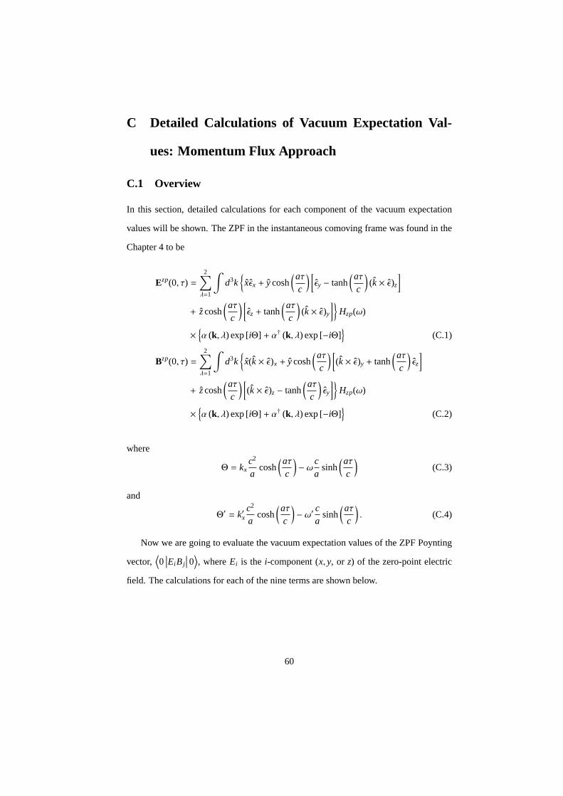
C Detailed Calculations of Vacuum Expectation Val-

ues: Momentum Flux Approach

C.1 Overview

In this section, detailed calculations for each component of the vacuum expectation

values will be shown. The ZPF in the instantaneous comoving frame was found in the

Chapter 4 to be

Ezp(0, τ) =

2∑

λ=1

∫d3k

xεx + ycosh

(aτc

) [εy − tanh

(aτc

)(k× ε)z

]

+ zcosh(aτ

c

) [εz + tanh

(aτc

)(k× ε)y

]Hzp(ω)

×α (k, λ) exp [iΘ] + α† (k, λ) exp [−iΘ]

(C.1)

Bzp(0, τ) =

2∑

λ=1

∫d3k

x(k× ε)x + ycosh

(aτc

) [(k× ε)y + tanh

(aτc

)εz

]

+ zcosh(aτ

c

) [(k× ε)z − tanh

(aτc

)εy

]Hzp(ω)

×α (k, λ) exp [iΘ] + α† (k, λ) exp [−iΘ]

(C.2)

where

Θ = kxc2

acosh

(aτc

)− ωc

asinh

(aτc

)(C.3)

and

Θ′ = k′xc2

acosh

(aτc

)− ω′ c

asinh

(aτc

). (C.4)

Now we are going to evaluate the vacuum expectation values of the ZPF Poynting

vector,⟨0∣∣∣Ei Bj

∣∣∣ 0⟩, whereEi is the i-component (x, y, or z) of the zero-point electric

field. The calculations for each of the nine terms are shown below.

60

C.2 Evaluation of Each Component

C.2.1 〈0 |ExBx| 0〉

In order to evaluate the component〈0 |ExBx|0〉, the product of thex-components of the

ZPF operators (C.1) and (C.2) is formed first and we obtain

〈0 |ExBx|0〉 =

2∑

λ=1

2∑

λ′=1

∫d3k

∫d3k′εx(k

′ × ε′)xH2zp(ω)

⟨0∣∣∣∣α (k, λ) exp[iΘ] + α† (k, λ) exp[−iΘ]

×α(k′, λ′

)exp[iΘ′] + α†

(k′, λ′

)exp[−iΘ′]

∣∣∣∣ 0⟩, (C.5)

where

Θ = kxc2

acosh

(aτc

)− ωc

asinh

(aτc

)(C.6)

and

Θ′ = k′xc2

acosh

(aτc

)− ω′ c

asinh

(aτc

). (C.7)

The expression above has four terms. However, only the term proportional to⟨0∣∣∣α (k, λ) , α† (k′, λ′)

∣∣∣ 0⟩

remains as in (C.10), and the above expression is simplified

to

〈0 |ExBx|0〉 =

2∑

λ=1

2∑

λ′=1

∫d3k

∫d3k′εx(k

′ × ε′)xH2zp(ω)

×⟨0∣∣∣α (k, λ) , α†

(k′, λ′

)∣∣∣ 0⟩

exp [iΘ(k)] exp[−iΘ′(k′)

], (C.8)

with the use of the expectation values

⟨0∣∣∣α (k, λ) , α

(k′, λ′

)∣∣∣ 0⟩

=⟨0∣∣∣α† (k, λ) , α†

(k′, λ′

)∣∣∣ 0⟩

= 0 (C.9)⟨0∣∣∣α (k, λ) , α†

(k′, λ′

)∣∣∣ 0⟩

= δλ,λ′δ3 (

k − k′)

(C.10)⟨0∣∣∣α† (k, λ) , α

(k′, λ′

)∣∣∣ 0⟩

= 0. (C.11)

61

Since the term in the second line in (C.8) isδλ,λ′δ3 (k − k′) exp[iΘ(k)] exp [−iΘ′(k′)],

Eq.(C.8) becomes

〈0 |ExBx|0〉 =

2∑

λ=1

2∑

λ′=1

∫d3k

∫d3k′εx(k

′ × ε′)xH2zp(ω)

×δλ,λ′δ3 (k − k′

)exp[iΘ(k)] exp

[−iΘ′(k′)], (C.12)

which, after one integration over thek-sphere, reduces to

〈0 |ExBx|0〉 =

2∑

λ=1

∫d3kεx(k× ε)xH

2zp(ω). (C.13)

With a use of the polarization formula, we find that

2∑

λ=1

εx(k× ε)x =∑

k=x,y,z

εiik kk = 0, (C.14)

and after substituting this result into the equation above, it is concluded that〈0 |ExBx|0〉 =

0.

C.2.2⟨0∣∣∣ExBy

∣∣∣ 0⟩

⟨0∣∣∣ExBy

∣∣∣ 0⟩

can also be evaluated in the similar manner as〈0 |ExBx|0〉. That is, the

product of thex−component of the electric field and they−component of the magnetic

field is formed, which involves two sums and two integrals as in (C.5). Then, the

expectation value is taken as before, leaving

⟨0∣∣∣ExBy

∣∣∣ 0⟩

=

2∑

λ=1

∫d3kH2

zp(ω)εx coshaτc

[(k× ε)y + tanh

aτcεz

](C.15)

62

In order to evaluate this equation, we use the following polarization formulae again:

2∑

λ=1

εx(k× ε)y = kz, (C.16)

2∑

λ=1

εxεy = −kxkz, (C.17)

and obtain

⟨0∣∣∣ExBy

∣∣∣ 0⟩

=

2∑

λ=1

∫d3kH2

zp(ω)[cosh

aτc

kz − sinhaτc

kxkz

]. (C.18)

The above expression can be evaluated by integrating over thek−sphere using the re-

lation, ∫d3k =

∫k2dk

∫dΩ =

∫k2dk

∫sinθdθ

∫dφ. (C.19)

On applying this relation, the first term including thekz term gives

∫d3kkz =

∫k2dk

∫sinθ cosθdθ

∫dφ = 0, (C.20)

since the angular integration∫

sinθ cosθdθ is zero. Similarly, the second term involv-

ing thekxkz reduces to

∫d3kkxkz =

∫k2dk

∫sin2 θ cosθdθ

∫cosφdφ = 0, (C.21)

due to the vanishing azimuthal integration∫

cosφdφ, and it is concluded that⟨0∣∣∣ExBy

∣∣∣ 0⟩

is also zero.

C.2.3 〈0 |ExBz|0〉

We continue the same analysis on other components. For〈0 |ExBz| 0〉, we obtain

〈0 |ExBz|0〉 =

2∑

λ=1

∫d3kH2

zp(ω)εx

[cosh

aτc

(k× ε)z − sinhaτcεy

]. (C.22)

63

Again, we make use of the polarization equations,

2∑

λ=1

εx(k× ε)z = −ky (C.23)

2∑

λ=1

εxεy = −kxky, (C.24)

and obtain

〈0 |ExBz|0〉 =

2∑

λ=1

∫d3kH2

zp(ω)[sinh

aτc

ky − coshaτc

kxky

]. (C.25)

After thek−sphere integration, the two terms in the above equation reduce to

∫d3kky =

∫k2dk

∫sin2 θdθ

∫sinφdφ = 0, (C.26)

and ∫d3kkxky =

∫k2dk

∫sin3 θdθ

∫sinφ cosφdφ = 0, (C.27)

both due to the vanishing azimuthal integrations, and it is concluded that〈0 |ExBz|0〉 is

also zero. This is actually a well expected result. Since it is assumed that the object is

accelerating along thex−axis, there should exist a symmetry about this direction, and

the value of〈0 |ExBz|0〉 should be the same as that of⟨0∣∣∣ExBy

∣∣∣ 0⟩.

C.2.4⟨0∣∣∣EyBx

∣∣∣ 0⟩

⟨0∣∣∣EyBx

∣∣∣ 0⟩

=

2∑

λ=1

∫d3kH2

zp(ω)[cosh

aτcεy − sinh

aτc

(k× ε)z

](k× ε)x. (C.28)

We make use of the following polarization equations,

2∑

λ=1

εy(k× ε)x = −kz, (C.29)

2∑

λ=1

(k× ε)z(k× ε)x = −kxkz. (C.30)

64

Since, as we have seen before, both terms disappear after the integrations,

∫d3kkz = 0, (C.31)

and ∫d3kkxkz = 0, (C.32)

it is concluded that⟨0∣∣∣EyBx

∣∣∣ 0⟩

= 0. (C.33)

C.2.5⟨0∣∣∣EyBy

∣∣∣ 0⟩

⟨0∣∣∣EyBy

∣∣∣ 0⟩

=

2∑

λ=1

∫d3kH2

zp(ω)

×[cosh

aτcεy − sinh

aτc

(k× ε)z

] [cosh

aτc

(k× ε)y + sinhaτcεz

]. (C.34)

This equation has four terms, and each of them are to be obtained with the use of the

following polarization equations:

2∑

λ=1

εy(k× ε)y = 0

2∑

λ=1

(k× ε)z(k× ε)y = −kykz

2∑

λ=1

εyεz = −kykz

2∑

λ=1

(k× ε)zεz = 0.

With these results, it is shown that,

⟨0∣∣∣EyBy

∣∣∣ 0⟩

=

2∑

λ=1

∫d3kH2

zp(ω)[cosh

aτc

sinhaτc

](kykz − kykz) = 0. (C.35)

65

C.2.6⟨0∣∣∣EyBz

∣∣∣ 0⟩

⟨0∣∣∣EyBz

∣∣∣ 0⟩

=

2∑

λ=1

∫d3kH2

zp(ω)

×[cosh

aτcεy − sinh

aτc

(k× ε)z

] [cosh

aτc

(k× ε)z − sinhaτcεy

]. (C.36)

This equation also has four terms. We evaluate these using the following polarization

equations,

2∑

λ=1

εy(k× ε)z = kx

2∑

λ=1

(k× ε)z(k× ε)z = k2x + k2

y = 1− k2z

2∑

λ=1

ε2y = 1− k2

y.

Combining the above results, it is shown that,

⟨0∣∣∣EyBz

∣∣∣ 0⟩

=

∫d3kH2

zp(ω)

×[

cosh2aτc

+ sinh2 aτc

]kx − cosh

aτc

sinhaτc

[(1− k2

z) + (1− k2y)]

=

∫d3kH2

zp(ω)[

cosh2aτc

+ sinh2 aτc

]kx − cosh

aτc

sinhaτc

[2− k2

y − k2z

].

(C.37)

Using the relation,

1 = k2x + k2

y + k2z, (C.38)

the above expectation value can be simplified as,

⟨0∣∣∣EyBz

∣∣∣ 0⟩

=

∫d3kH2

zp(ω)[

cosh2aτc

+ sinh2 aτc

]kx − cosh

aτc

sinhaτc

[1 + k2

x

].

(C.39)

66

The first term of this equation is zero since∫

d3kkx = 0, and we obtain,

⟨0∣∣∣EyBz

∣∣∣ 0⟩

= −∫

d3kH2zp(ω) cosh

aτc

sinhaτc

[1 + k2

x

]. (C.40)

After substituting

H2zp(ω) =

~ω

4π2, (C.41)

dk = dω/c, (C.42)

and,

sinhθ coshθ =12

sinh(2θ), (C.43)

we obtain,

⟨0∣∣∣EyBz

∣∣∣ 0⟩

= −12

sinh2aτc

∫dω

~ω3

4π2c3

∫dΩ

(1 + k2

x

). (C.44)

The angle integrations in the above equation gives

∫dΩ =

∫sinθdθdφ = 4π

∫k2

xdΩ =

∫sin3 θdθ

∫cosφdφ =

4π3

after minimal algebra, and the expectation value is found to be

⟨0∣∣∣EyBz

∣∣∣ 0⟩

= −4π3

sinh2aτc

∫~ω3

2π2c3dω. (C.45)

C.2.7 〈0 |EzBx|0〉

Due to symmetry about the direction of acceleration, i.e., thex−axis, the value of

67

〈0 |EzBx|0〉 should be the same as that of⟨0∣∣∣EyBx

∣∣∣ 0⟩. Therefore, it is concluded that

〈0 |EzBx|0〉 = 0. (C.46)

C.2.8⟨0∣∣∣EzBy

∣∣∣ 0⟩

The value of⟨0∣∣∣EzBy

∣∣∣ 0⟩

should be proportional to that of⟨0∣∣∣EyBz

∣∣∣ 0⟩, due to the

symmetry around thex−axis. This is found from the equation

⟨0∣∣∣EzBy

∣∣∣ 0⟩

=

2∑

λ=1

∫d3kH2

zp(ω)

×[cosh

aτcεz + sinh

aτc

(k× ε)y

] [cosh

aτc

(k× ε)y + sinhaτcεz

](C.47)

with the polarization equations,

2∑

λ=1

εz(k× ε)y = −kx

2∑

λ=1

(k× ε)y(k× ε)y = k2x + k2

z = 1− k2y

2∑

λ=1

ε2z = 1− k2

z.

Combining the above results, it is shown that,

⟨0∣∣∣EzBy

∣∣∣ 0⟩

=

∫d3kH2

zp(ω)

×−

[cosh2

aτc

+ sinh2 aτc

]kx + cosh

aτc

sinhaτc

[(1− k2

y) + (1− k2z)]. (C.48)

Since the angle integration for the first term is zero as we have seen in the case of⟨0∣∣∣EyBz

∣∣∣ 0⟩, we have

⟨0∣∣∣EzBy

∣∣∣ 0⟩

=

∫d3kH2

zp(ω) coshaτc

sinhaτc

[1 + k2

x

]. (C.49)

68

It is found that this is the same expression as the Eq(C.40) for⟨0∣∣∣EyBz

∣∣∣ 0⟩, except

the absence of the negative sign. Therefore, we conclude that

⟨0∣∣∣EzBy

∣∣∣ 0⟩

=4π3

sinh2aτc

∫~ω3

2π2c3dω, (C.50)

which is also the same value as⟨0∣∣∣EyBz

∣∣∣ 0⟩

(Eq.C.45), except the opposite sign.

C.2.9 〈0 |EzBz|0〉

Due to the cylindrical symmetry around thex−axis, the value of〈0 |EzBz|0〉 should

vanish as in the case of⟨0∣∣∣EyBy

∣∣∣ 0⟩. Hence

〈0 |EzBz|0〉 = 0. (C.51)

69

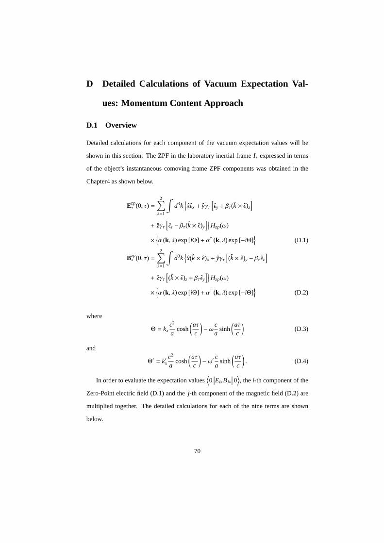
D Detailed Calculations of Vacuum Expectation Val-

ues: Momentum Content Approach

D.1 Overview

Detailed calculations for each component of the vacuum expectation values will be

shown in this section. The ZPF in the laboratory inertial frameI∗ expressed in terms

of the object’s instantaneous comoving frame ZPF components was obtained in the

Chapter4 as shown below.

Ezp∗ (0, τ) =

2∑

λ=1

∫d3k

xεx + yγτ

[εy + βτ(k× ε)z

]

+ zγτ[εz − βτ(k× ε)y

]Hzp(ω)

×α (k, λ) exp [iΘ] + α† (k, λ) exp [−iΘ]

(D.1)

Bzp∗ (0, τ) =

2∑

λ=1

∫d3k

x(k× ε)x + yγτ

[(k× ε)y − βτεz

]

+ zγτ[(k× ε)z + βτεy

]Hzp(ω)

×α (k, λ) exp [iΘ] + α† (k, λ) exp [−iΘ]

(D.2)

where

Θ = kxc2

acosh

(aτc

)− ωc

asinh

(aτc

)(D.3)

and

Θ′ = k′xc2

acosh

(aτc

)− ω′ c

asinh

(aτc

). (D.4)

In order to evaluate the expectation values⟨0∣∣∣Ei∗Bj∗

∣∣∣ 0⟩, thei-th component of the

Zero-Point electric field (D.1) and thej-th component of the magnetic field (D.2) are

multiplied together. The detailed calculations for each of the nine terms are shown

below.

70

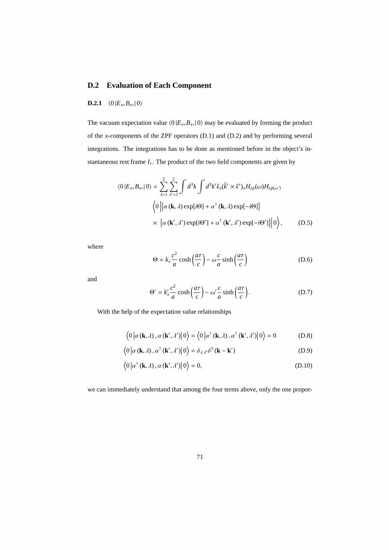
D.2 Evaluation of Each Component

D.2.1 〈0 |Ex∗Bx∗|0〉

The vacuum expectation value〈0 |Ex∗Bx∗|0〉 may be evaluated by forming the product

of the x-components of the ZPF operators (D.1) and (D.2) and by performing several

integrations. The integrations has to be done as mentioned before in the object’s in-

stantaneous rest frameIτ. The product of the two field components are given by

〈0 |Ex∗Bx∗| 0〉 =

2∑

λ=1

2∑

λ′=1

∫d3k

∫d3k′εx(k

′ × ε′)xHzp(ω)Hzp(ω′)

⟨0∣∣∣∣α (k, λ) exp[iΘ] + α† (k, λ) exp[−iΘ]

×α(k′, λ′

)exp[iΘ′] + α†

(k′, λ′

)exp[−iΘ′]

∣∣∣∣ 0⟩, (D.5)

where

Θ = kxc2

acosh

(aτc

)− ωc

asinh

(aτc

)(D.6)

and

Θ′ = k′xc2

acosh

(aτc

)− ω′ c

asinh

(aτc

). (D.7)

With the help of the expectation value relationships

⟨0∣∣∣α (k, λ) , α

(k′, λ′

)∣∣∣ 0⟩

=⟨0∣∣∣α† (k, λ) , α†

(k′, λ′

)∣∣∣ 0⟩

= 0 (D.8)⟨0∣∣∣α (k, λ) , α†

(k′, λ′

)∣∣∣ 0⟩

= δλ,λ′δ3 (

k − k′)

(D.9)⟨0∣∣∣α† (k, λ) , α

(k′, λ′

)∣∣∣ 0⟩

= 0, (D.10)

we can immediately understand that among the four terms above, only the one propor-

71

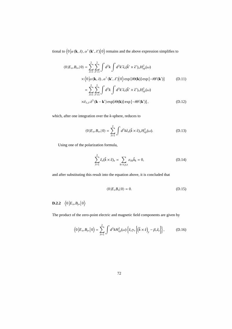
tional to⟨0∣∣∣α (k, λ) , α† (k′, λ′)

∣∣∣ 0⟩

remains and the above expression simplifies to

〈0 |Ex∗Bx∗| 0〉 =

2∑

λ=1

2∑

λ′=1

∫d3k

∫d3k′εx(k

′ × ε′)xH2zp(ω)

×⟨0∣∣∣α (k, λ) , α†

(k′, λ′

)∣∣∣ 0⟩

exp [iΘ(k)] exp[−iΘ′(k′)

](D.11)

=

2∑

λ=1

2∑

λ′=1

∫d3k

∫d3k′εx(k

′ × ε′)xH2zp(ω)

×δλ,λ′δ3 (k − k′

)exp[iΘ(k)] exp

[−iΘ′(k′)], (D.12)

which, after one integration over thek-sphere, reduces to

〈0 |Ex∗Bx∗|0〉 =

2∑

λ=1

∫d3kεx(k× ε)xH

2zp(ω). (D.13)

Using one of the polarization formula,

2∑

λ=1

εx(k× ε)x =∑

k=x,y,z

εiik kk = 0, (D.14)

and after substituting this result into the equation above, it is concluded that

〈0 |ExBx|0〉 = 0. (D.15)

D.2.2⟨0∣∣∣Ex∗By∗

∣∣∣ 0⟩

The product of the zero-point electric and magnetic field components are given by

⟨0∣∣∣Ex∗By∗

∣∣∣ 0⟩

=

2∑

λ=1

∫d3kH2

zp(ω)εxγτ

[(k× ε

)y− βτεz

], (D.16)

72

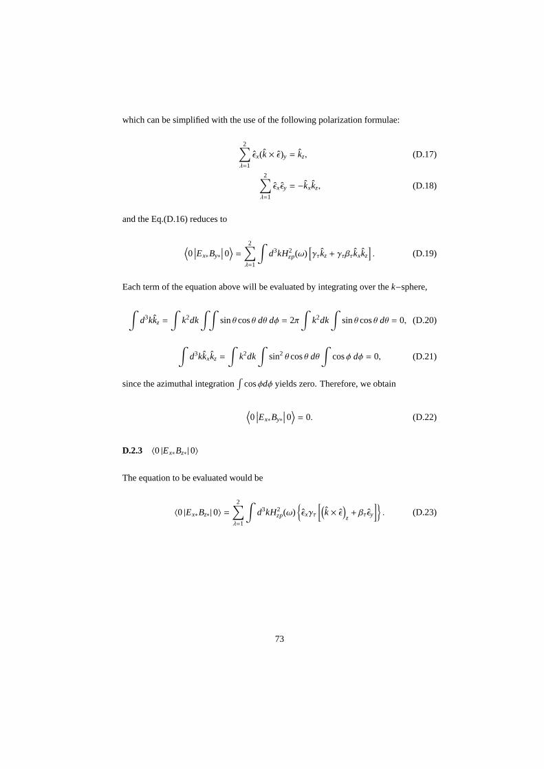
which can be simplified with the use of the following polarization formulae:

2∑

λ=1

εx(k× ε)y = kz, (D.17)

2∑

λ=1

εxεy = −kxkz, (D.18)

and the Eq.(D.16) reduces to

⟨0∣∣∣Ex∗By∗

∣∣∣ 0⟩

=

2∑

λ=1

∫d3kH2

zp(ω)[γτkz + γτβτkxkz

]. (D.19)

Each term of the equation above will be evaluated by integrating over thek−sphere,

∫d3kkz =

∫k2dk

∫ ∫sinθ cosθ dθ dφ = 2π

∫k2dk

∫sinθ cosθ dθ = 0, (D.20)

∫d3kkxkz =

∫k2dk

∫sin2 θ cosθ dθ

∫cosφ dφ = 0, (D.21)

since the azimuthal integration∫

cosφdφ yields zero. Therefore, we obtain

⟨0∣∣∣Ex∗By∗

∣∣∣ 0⟩

= 0. (D.22)

D.2.3 〈0 |Ex∗Bz∗|0〉

The equation to be evaluated would be

〈0 |Ex∗Bz∗|0〉 =

2∑

λ=1

∫d3kH2

zp(ω)εxγτ

[(k× ε

)z+ βτεy

]. (D.23)

73

The polarization equations used for this are

2∑

λ=1

εx

(k× ε

)z

= −ky (D.24)

2∑

λ=1

εxεy = −kxky, (D.25)

and the Eq.(D.23) simplifies to

〈0 |Ex∗Bz∗|0〉 =

2∑

λ=1

∫d3kH2

zp(ω)[γτky + βτkxky

]. (D.26)

Again we perform thek−sphere integration and obtain

∫d3kky =

∫k2dk

∫sin2 θ dθ

∫sinφ dφ = 0, (D.27)

and ∫d3kkxky =

∫k2dk

∫sin3 θ dθ

∫sinφ cosφ dφ = 0. (D.28)

Both integrations are zero due to the vanishing azimuthal integrations, and we obtain

again

〈0 |Ex∗Bz∗|0〉 = 0. (D.29)

Since the object is moving in the positivex-direction, there exists a symmetry about

x-axis. Therefore, it is reasonable that we have obtained the same values for both⟨0∣∣∣Ex∗By∗

∣∣∣ 0⟩

and〈0 |Ex∗Bz∗|0〉.

D.2.4⟨0∣∣∣Ey∗Bx∗

∣∣∣ 0⟩

After multiplying they-component of the ZPF electric field by thex-component of the

magnetic field, we obtain

⟨0∣∣∣Ey∗Bx∗

∣∣∣ 0⟩

=

2∑

λ=1

∫d3kH2

zp(ω)γτ

[εy + βτ

(k× ε

)z

] (k× ε

)x

. (D.30)

74

The use of the following polarization equations,

2∑

λ=1

εy(k× ε)x = −kz, (D.31)

2∑

λ=1

(k× ε)z(k× ε)x = −kxkz, (D.32)

yields the samek-sphere integration (D.20) and (D.21) already evaluated previously.

Hence, we conclude⟨0∣∣∣Ey∗Bx∗

∣∣∣ 0⟩

= 0. (D.33)

D.2.5⟨0∣∣∣Ey∗By∗

∣∣∣ 0⟩

⟨0∣∣∣Ey∗By∗

∣∣∣ 0⟩

=

2∑

λ=1

∫d3kH2

zp(ω)

×[γτεy + βτ

(k× ε

)z

] [γτ

(k× ε

)y− βτεz

](D.34)

Among the four terms in the equation above, two terms immediately reduce to zero

upon application of the polarization formula:

2∑

λ=1

εy(k× ε

)y

= 0

2∑

λ=1

(k× ε

)zεz = 0,

and the Eq.(D.34) simplifies to

⟨0∣∣∣Ey∗By∗

∣∣∣ 0⟩

=

2∑

λ=1

∫d3kH2

zp(ω) × γ2τβτ

[−εyεz +

(k× ε

)z

(k× ε

)y

]. (D.35)

Applying the polarization equations again, it is found that the non-vanishing two terms

75

have values

2∑

λ=1

(k× ε

)z

(k× ε

)y

= −kykz,

−2∑

λ=1

εyεz = kykz,

which exactly cancels each other. to conclude that

⟨0∣∣∣Ey∗By∗

∣∣∣ 0⟩

= 0. (D.36)

D.2.6⟨0∣∣∣Ey∗Bz∗

∣∣∣ 0⟩

⟨0∣∣∣Ey∗Bz∗

∣∣∣ 0⟩

=

2∑

λ=1

∫d3kH2

zp(ω)

×γτ[εy + βτ

(k× ε

)z

]γτ

[(k× ε

)z+ βτεy

]. (D.37)

This equation also has four terms, but two of them yield the samek-sphere integrations

we have already evaluated:

2∑

λ=1

εy(k× ε

)z

=

2∑

λ=1

(k× ε

)zεy = kx,

which gives zero after thek integration,

∫d3kkx =

∫k2dk

∫sin2 θ dθ

∫cosφ dφ = 0. (D.38)

76

The remaining two terms have values

2∑

λ=1

(k× ε

)z

(k× ε

)z

= 1− k2z

2∑

λ=1

ε2y = 1− k2

y.

Then the Eq.(D.37) simplifies to

⟨0∣∣∣Ey∗Bz∗

∣∣∣ 0⟩

=

2∑

λ=1

∫d3kH2

zp(ω)γ2τβτ

[εyεy +

(k× ε

)z

(k× ε

)z

]

=

∫d3kH2

zp(ω)γ2τβτ

(2− k2

y − k2z

)

=

∫d3kH2

zp(ω)γ2τβτ

(1 + k2

x

)(D.39)

where the relation 1= k2x + k2

y + k2z was used in the last step. Thek-integrations are

given below as

∫d3k =

∫k2dk

∫dΩ = 4π

∫k2dk

∫d3kk2

x =

∫k2dk

∫k2

xdΩ =

∫k2dk

∫sin3 θdθ

∫cosφdφ =

4π3

∫k2dk

after minimal algebra, to further simplify the Eq.(D.39) to

⟨0∣∣∣Ey∗Bz∗

∣∣∣ 0⟩

=16π3

∫k2dkH2

zp(ω)γ2τβτ. (D.40)

Upon changing the variable of integration fromk toω and substituting the value of the

spectral function, we can finally obtain

⟨0∣∣∣Ey∗Bz∗

∣∣∣ 0⟩

=8π3

sinh2aτc

∫~ω3

4π2c3dω. (D.41)

77

where the relation

γ2τβτ = cosh2

aτc

tanhaτc

= sinhaτc

coshaτc

=12

sinh2aτc

(D.42)

was used.

D.2.7 〈0 |Ez∗Bx∗|0〉

〈0 |Ez∗Bx∗|0〉 =

2∑

λ=1

∫d3kH2

zp(ω)γτ[εz − βτ

(k× ε

)y

] (k× ε

)x

(D.43)

with the polarization equations,

2∑

λ=1

εz(k× ε

)x

= ky

2∑

λ=1

(k× ε

)y

(k× ε

)x

= −kxky

reduces to

〈0 |Ez∗Bx∗| 0〉 =

∫k2dkH2

zp(ω)γτ[ky + βτkxky

]. (D.44)

These angular integrations have already been found in Eq.(D.27) and Eq.(D.28) to be

zero. Therefore, we conclude that

〈0 |Ez∗Bx∗|0〉 = 0. (D.45)

This result is also expected due to symmetry about thex−axis, the direction of the

objects accelerated motion. Hence the value of〈0 |Ez∗Bx∗| 0〉 should be the same as that

of⟨0∣∣∣Ey∗Bx∗

∣∣∣ 0⟩, which is zero.

D.2.8⟨0∣∣∣Ez∗By∗

∣∣∣ 0⟩

Once again due to the symmetry around thex−axis, the value of⟨0∣∣∣Ez∗By∗

∣∣∣ 0⟩

should

78

be at least proportional to that of⟨0∣∣∣Ey∗Bz∗

∣∣∣ 0⟩.⟨0∣∣∣Ez∗By∗

∣∣∣ 0⟩

is expressed as

⟨0∣∣∣Ez∗By∗

∣∣∣ 0⟩

=

2∑

λ=1

∫d3kH2

zp(ω)

×γτ[εz − βτ

(k× ε

)y

]γτ

[(k× ε

)y− βτεz

], (D.46)

which can be simplified with the polarization equations,

2∑

λ=1

εz(k× ε

)y

= −kx

2∑

λ=1

(k× ε

)y

(k× ε

)y

= k2x + k2

z = 1− k2y

2∑

λ=1

ε2z = 1− k2

z.

The first equation above reduces to zero after the angular integration Eq.(D.38).

Substituting the other two results, Eq.(D.46) simplifies to

⟨0∣∣∣Ez∗By∗

∣∣∣ 0⟩

=

∫d3kH2

zp(ω)(−γ2

τβτ) [(

1− k2y

)+

(1− k2

z

)]

=

∫d3kH2

zp(ω)(−γ2

τβτ) [

1 + k2x

], (D.47)

where we have used the relation 1= k2x + k2

y + k2z in the last step. As expected, we

obtain the same expression as the Eq(D.39) in⟨0∣∣∣Ey∗Bz∗

∣∣∣ 0⟩, except the absence of the

negative sign. Therefore, we conclude that

⟨0∣∣∣Ez∗By∗

∣∣∣ 0⟩

= −⟨0∣∣∣Ey∗Bz∗

∣∣∣ 0⟩

=8π3

sinh2aτc

∫~ω3

4π2c3dω. (D.48)

As mentioned in the main text, only⟨0∣∣∣Ey∗Bz∗

∣∣∣ 0⟩

and⟨0∣∣∣Ez∗By∗

∣∣∣ 0⟩

remain non-vanishing

and the other seven terms reduce to zero.

79

D.2.9 〈0 |Ez∗Bz∗|0〉

The value of〈0 |Ez∗Bz∗|0〉 should vanish as in the case of⟨0∣∣∣Ey∗By∗

∣∣∣ 0⟩, for there exists

a cylindrical symmetry around the motion of the object, i.e.,x−axis.

〈0 |Ez∗Bz∗|0〉 =

2∑

λ=1

∫d3kH2

zp(ω)

×γτ[εz − βτ

(k× ε

)y

]γτ

[(k× ε

)z+ βτεy

](D.49)

Two of the four terms in the equation above can be found immediately as zero after the

polarization formula,

2∑

λ=1

εz(k× ε

)z

= 0

2∑

λ=1

(k× ε

)yεy = 0.

The remaining two terms turn out to be

2∑

λ=1

(k× ε

)y

(k× ε

)z

= −kykz,

and2∑

λ=1

εzεy = −kykz.

These two terms, however, cancel each other and as expected, we have

〈0 |Ez∗Bz∗|0〉 =

2∑

λ=1

∫d3kH2

zp(ω)γ2τβτ

[−

(k× ε

)y

(k× ε

)z+ εzεy

]

=

∫d3kH2

zp(ω)γ2τβτ

[kykz − kykz

]

= 0. (D.50)

This result also confirms the fact thatE · B = 0.

80

E Derivation of the Momentum Four-Vector of the Elec-

tromagnetic Field

In this section, the expressions for the four-momentum (5.15)–(5.17), that is

Pµ =

(1c

W,P)

(E.1)

with

W = γ

∫Udσ − γβ

c

∫S · ndσ (E.2)

and

P =γ

c2

∫Sdσ +

γβ

c

∫ ←→T · ndσ. (E.3)

are going to be derived. For this purpose, we start from the quantity

Pµ ≡ 1c

∫Θµνdσν, (E.4)

the integration of the electromagnetic energy tensor over a spacelike surfaceσ given

by the equation

nµxµ + cτ = 0, (E.5)

wherenµ is the unit normal vector of the plane, which is necessarily timelike,

nµnµ = −1. (E.6)

Also by taking the derivative of (E.5), we obtain

nµ = −c∂µτ and nµ =dxµ

cdτ. (E.7)

81

As explained earlier, any instant of an inertial observer is characterized by this space-

like planeσ and the unit normalnν, and the surface element is given by

dσµ = nµdσ, (E.8)

with the invariant area element

dσ = −nµdσµ = dxdydz. (E.9)

For the evaluation of the zero-component of the momentum four-vector, we start

from the definition (E.1) and obtain

P0 =1c

∫Θ0νdσν =

1c

[∫Θ00n0dσ +

∫Θ0knkdσ

], (E.10)

where (E.8) was used. In the case of our interest where the object is moving in the

positivex-direction with velocityv, the normal surface is given bynν = (γ; γβn), and

the above equation becomes

P0 =1c

[∫(−U)(−γ)dσ +

∫ (− 1

4π

)(E × B)k γβnkdσ

](E.11)

after substituting the energy-momentum tensor elements

Θ00 =18π

(E2 + B2

)≡ −U, (E.12)

and

Θ0i = − 14π

(E × B)i , (E.13)

whereU is the electromagnetic energy density. With the identification of the Poynting

vector

S≡ c4π

(E × B) , (E.14)

82

the quantity inside the square bracket becomes

W =

∫γUdσ −

∫ (γβ

c

)S · ndσ, (E.15)

which yields our expected results,

P0 ≡ 1c

W (E.16)

with

W = γ

∫Udσ − γβ

c

∫S · ndσ. (E.17)

The space part of the momentum four-vector can be derived in a similar manner.

We start again from the definition (E.1) and obtain

Pi =1c

∫Θiνdσν =

1c

[∫Θi0n0dσ +

∫Θi j n jdσ

], (E.18)

where we have used (E.8). Substituting the space-time mixed elements (E.13) and the

space elements of the tensor

Θi j = Ti j =14π

[EiE j + Bi Bj − 1

2(E2 + B2)δi j

], (E.19)

Eq.(E.18) becomes

Pi =1c

[−

∫14π

(E × B)i (−γ)dσ +

∫Ti jγβn jdσ

]

=1c

[γ

c

∫Sidσ + γβ

∫Ti · ndσ

]

=γ

c2

∫Sidσ +

γβ

c

∫Ti · ndσ. (E.20)

In the expression above,Ti is a row vector andi = x, y, z. Therefore, in vector notation,

83

we obtain the desired results

P =γ

c2

∫Sdσ +

γβ

c

∫T · ndσ. (E.21)

84

F Derivation of Davies-Unruh Effect

F.1 Overview

Davies-Unruh effect was discovered independently by Davies (1975)[20] and Unruh

(1976)[21] in their efforts to better understand the so-called black-hole evaporation in

the context of QED. Its remarkable result is summarized as follows: A system under-

going a uniform accelerationa behaves as if it were immersed in a thermal radiation of

temperatureT that is proportional to the magnitude of the acceleration, namely,

T =~a

2πkBc. (F.1)

It is hard to understand why an accelerating object sees a thermal radiation of tem-

perature proportional to acceleration, based on the idea of “empty” vacuum. However,

once it is realized that the vacuum is filled with ZPF, this Davies-Unruh effect could be

understood as a result of the interaction between the accelerating object and the ZPF.

Davies-Unruh effect has been derived in several different ways by Boyer[40, 18,

41], all in the context of SED. In this chapter, Boyer’s first method[40] is followed

using the two-point correlation function (expectation value), but instead of SED, it is

performed in the quantum formulation.8 First, the correlation function for an object

accelerated in ZPF is evaluated, and this value is compared with the value of another

correlation function obtained for random thermal radiation of temperatureT. By com-

parison of two expectation values, we can obtain the relationship between the acceler-

ationa of the object and the temperatureT of the thermal radiation.

As a basis of this analysis, we adopt a hyperbolic motion[29, 30], in which an object

is under constant acceleration.9 The accelerating object is moving in the positivex-

direction, and in its own rest frameS, the object is at rest at a point (c2/a,0,0), which

8A similar derivation in the case of a scalar field is also found in Milonni[42], Sec. 2.10.9For more detailed descriptions of the hyperbolic motion, refer to Sec. 4.2.

85

coincides with the laboratory inertial frameI∗ at τ = t = 0. The space and time

coordinates of the object in the laboratory frameI∗ is related to the proper timeτ in the

following way:

t∗ =ca

sinh(aτ

c

),

x∗ =c2

acosh

(aτc

),

y∗ = 0,

z∗ = 0, (F.2)

and also,

βτ =u∗(τ)

c=

1c

dx∗dt∗

=1c

dx∗/dτdt∗/dτ

= tanh(aτ

c

), (F.3)

and

γτ =1√

1− β2τ

=1

sech(aτ/c)= cosh

(aτc

). (F.4)

F.2 Massless Scalar Field

F.2.1 ZPF in a Massless Scalar Field

For a massless scalar field, the ZPF can be expressed as an expansion of plane waves

with random phases:

φ(r , t) =

∫d3k fq(ω)

[α(k) exp(−iωt + ik · r ) + α†(k) exp(iωt − ik · r )

], (F.5)

86

where fq(ω) is the spectral function introduced to set the scale of ZPF, and has the

value,10

f 2q (ω) =

~c2

4π2ω. (F.6)

Also,α(k) andα†(k) are annihilation and creation operators, which follow the com-

mutation rules

[α(k1), α(k2)] =[α†(k1), α†(k2)

]= 0 (F.7)

[α(k1), α†(k2)

]= δ3(k1 − k2) (F.8)

and have the expectation values,

〈0 |α(k1) α(k2)|0〉 =⟨0∣∣∣α†(k1) α†(k2)

∣∣∣ 0⟩

= 0, (F.9)⟨0∣∣∣α(k1) α†(k2)

∣∣∣ 0⟩

= δ3 (k1 − k2) , (F.10)⟨0∣∣∣α†(k1) α(k2)

∣∣∣ 0⟩

= 0. (F.11)

The overline onφ in Eq.(F.5) indicates that this field is expressed in operators.

Notice the absence of the polarization vectors in the case of scalar field, as compared

to the ordinary vector field such as Eq.(2.12) and Eq.(2.13).

F.2.2 Expectation Value for an Accelerating Object in Random Zero-Point Ra-

diation

Now we like to evaluate the expectation values in the field fluctuations at a pointr in

space, which characterizes the random radiation field. For this purpose, we construct

10In the reference[40], Boyer usesf0(ω) = ~c2/2π2ω for the classical case, and in the quantum case, extrafactor of 1/2 is inserted to the expression for the field, Eq.(F.5) with the samef0(ω). However, it seems thatan extra factor of 1/

√2 would be more appropriate to attain the correspondence between the classical and

the quantum cases. In the present research, this extra factor of 1/√

2 is inserted in the functionfq(ω), so thatthe expression of the field remains unchanged in the quantum case except the use of quantum operators andthe exponential functions instead of cosine functions. For more details on this difference in the scaling factorbetween the classical and the quantum cases, refer to Appendix B.

87

the product of fields at the pointr and at two different timesσ − τ/2 andσ + τ/2, i.e.,

〈0 | ϕ(0, σ − τ/2) ϕ(0, σ + τ/2)|0〉.Since the ZPF spectrum is Lorentz-invariant, the fieldϕ(0, σ ± τ/2) at the location

of the object in the inertial frameIτ in which the object is instantaneously at rest may

be equivalent to the field in the laboratory frameI∗, whose space and time coordinates

are related to those inIτ frame by the Lorentz transformations (F.2), (F.3), and (F.4),

that is,

ϕ(0, σ ± τ/2) = φ

[c2

acosh

(a (σ ± τ/2)

c

),0,0,

ca

sinh

(a (σ ± τ/2)

c

)], (F.12)

whereφ is the field in the laboratory frameI∗, but the coordinates are given in terms of

the object’s proper timeτ.

It is to be noted that, since the field is expressed by field operators, in evaluating

the expectation value, the order of the operators does affect the result, which is not an

issue in the case of classical random radiation. Thus, to evaluate the expectation value,

we construct a symmetrized product of operators such that

〈0 | ϕ(r1, t1) ϕ(r2, t2)| 0〉‡ =12〈0 |ϕ(r1, t1) ϕ(r2, t2)|0〉 , (F.13)

where the double dagger on the left hand side of the equation indicates that the product

is yet to be symmetrized, andϕ(r1, t1) ϕ(r2, t2) inside the bracket on the right hand

side is an anti-commutator, defined as

ϕ(r1, t1) ϕ(r2, t2) = ϕ(r1, t1) ϕ(r2, t2) + ϕ(r2, t2) ϕ(r1, t1), (F.14)

yielding,

〈0 | ϕ(r1, t1) ϕ(r2, t2)|0〉‡ =12〈0 |ϕ(r1, t1) ϕ(r2, t2)| 0〉 + 〈0 |ϕ(r2, t2) ϕ(r1, t1)|0〉 ,

(F.15)

88

for the expectation value to be evaluated. Upon substituting the expression for the ZPF

from (F.5), we obtain for the first term of the equation above,

〈0 | ϕ(r1, t1) ϕ(r2, t2)|0〉 =

∫d3k1

∫d3k2 fq(ω1) fq(ω2)

×⟨0∣∣∣∣[α(k1)eiΘ1 + α†(k1)e−iΘ1

][α(k2)eiΘ2 + α†(k2)e−iΘ2

]∣∣∣∣ 0⟩,

(F.16)

where

Θ1 = k1 · r1 − ω1t1, (F.17)

Θ2 = k2 · r2 − ω2t2. (F.18)

This equation has four terms, but with the use of the relationship (F.9)- (F.11), three

terms are found to vanish and the expression simplifies to

〈0 | ϕ(r1, t1) ϕ(r2, t2)|0〉

=

∫d3k1

∫d3k2 fq(ω1) fq(ω2)eiΘ1e−iΘ2

⟨0∣∣∣α(k1)α†(k2)

∣∣∣ 0⟩

(F.19)

The expectation value yields a delta function ink, as shown in (F.10), which after

one integration overk reduces the expression above to

∫d3k f2

q (ω) exp [i (k · r1 − ωt1)] exp [−i (k · r2 − ωt2)]

=

∫d3k f2

q (ω) expi [k · (r1 − r2) − ω (t1 − t2)] . (F.20)

It is easy to show that, after following the same steps, the second term yields similar

89

result as (F.20):

∫d3k f2

q (ω) exp [i (k · r2 − ωt2)] exp [−i (k · r1 − ωt1)]

=

∫d3k f2

q (ω) exp−i [k · (r1 − r2) − ω (t1 − t2)] , (F.21)

with the only difference of (F.21) from (F.20) in the sign of the argument of the expo-

nential function. Therefore, after adding the two results above, the exponential func-

tions are replaced by a cosine, and the expectation value (F.15) becomes

〈0 | ϕ(r1, t1) ϕ(r2, t2)|0〉‡ =12〈0 |ϕ(r1, t1) ϕ(r2, t2)|0〉 + 〈0 |ϕ(r2, t2) ϕ(r1, t1)|0〉

=

∫d3k f2

q (ω) cos [k · (r1 − r2) − ω (t1 − t2)]

=

∫d3k

~c2

4π2ωcos [k · (r1 − r2) − ω (t1 − t2)] , (F.22)

where the value offq(ω) in (F.6) was inserted in the second equality. After substituting

the value ofr andt from (F.12), specifically

r1 =c2

acosh

(a(σ − τ/2)

c

), t1 =

ca

sinh

(a(σ − τ/2)

c

)(F.23)

r2 =c2

acosh

(a(σ + τ/2)

c

), t2 =

ca

sinh

(a(σ − τ/2)

c

), (F.24)

the above expression changes to

〈0 | ϕ(0, σ − τ/2) ϕ(0, σ + τ/2)|0〉‡

=

∫d3k

~c2

4π2ωcos

kx

c2

a

[cosh

(a(σ − τ/2)

c

)− cosh

(a(σ + τ/2)

c

)]

−ωca

[sinh

(a(σ − τ/2)

c

)− sinh

(a(σ + τ/2)

c

)]. (F.25)

This expression includes the proper timeσ in the argument of the cosine function.

However, since there is no preferred time in the hyperbolic motion, this dependence on

90

σ should vanish eventually, as will be shown below.

(F.25) can be more easily evaluated with the use of standard Lorentz transformation,

ω′ = ω cosh(aσ/c) − ckx sinh(aσ/c), (F.26)

k′x = kx cosh(aσ/c) − ωcsinh(aσ/c), (F.27)

k′y = ky, k′z = kz, (F.28)

and the Jacobian of the transformation

d3k = d3k′γ(1 + vk′x/ω′). (F.29)

With these transformations, we find that

d3kω

=d3k′γ(1 + vk′x/ω

′)γ(ω′ + vk′x)

=d3k′

ω′, (F.30)

and the expansion,

cosh(x) = 1 + x2/2! + · · · ' 1 + x2/2, (F.31)

sinh(x) = x + x3/3! + · · · ' x, (F.32)

together with (F.30) simplifies (F.25) as

〈0 | ϕ(0, σ − τ/2) ϕ(0, σ + τ/2)|0〉‡

=

∫~c2

4π2

d3k′

ω′cos

[2ω′

ca

sinh(aτ/2c)]. (F.33)

Note that this expression has noσ dependence as expected, for there is no preferred

91

time in hyperbolic motion. We integrate this equation over the angles using

∫d3k =

∫k2dk

∫dΩ = 4π

∫k2dk, (F.34)

and change the variable fromk toω = kc to obtain

〈0 | ϕ(0, σ − τ/2) ϕ(0, σ + τ/2)|0〉‡

=~

πc

∫dω′ω′ cos

[2ω′

ca

sinh(aτ/2c)]. (F.35)

This function is of the form

∫ ∞

0dx x cosbx = Re lim

λ−>0

∫ ∞

0dx x exp[(ib − λ)x]

= −b−2, (F.36)

and we can find the expectation value (F.33) to be

〈0 | ϕ(0, σ − τ/2) ϕ(0, σ + τ/2)|0〉‡ = − ~a2

4πc3csch2

(aτ2c

). (F.37)

F.2.3 Expectation Value for an Accelerating Object in Random Thermal Radia-

tion

We now explore the expectation value for a point detectorat restin a thermal radiation

field and compare this value with (F.37). It will be found that the two expectation

values agree ifT = ~a/2πkBc.

The object is at rest in its own inertial frame, and this time the surrounding field is

a random thermal radiation of temperatureT on top of the zero-point field. Therefore,

the object will see both the ZPF and the thermal radiation so that

f 2qT(ω) =

~c2

2ω

(12

+1

exp(~ω/kT) − 1

)=~c2

4ωcoth

(~ω

2kT

). (F.38)

92

The evaluation of the expectation value follows similar steps as the ones in the pre-

vious section: the product of the fields at two different timess±t/2,⟨0∣∣∣ φT(0, s− t/2) φT(0, s+ t/2)

∣∣∣ 0⟩‡

is constructed, and the expression for the scalar field (F.5) inserted. With the use of the

symmetrized operators (F.13), each of the two terms are shown to have similar forms

except the sign in the exponential functions, which transforms to a cosine function after

the addition. The argument of the hyperbolic sine function in (F.33) is further expanded

to obtain a simpler expression,

cos[2ω

ca

sinh(at/2c)]' cos

[2ω

ca

( at2c

)]' cos(ωt). (F.39)

Thus, for the expectation value of the object at rest in a thermal radiation, we obtain

⟨0∣∣∣ φT(0, s− t/2) φT(0, s+ t/2)

∣∣∣ 0⟩‡

=~

πc

∫ ∞

0dω ω coth

(~ω

2kT

)cosωt. (F.40)

We break up the integral into two parts using the identity,

coth

(~ω

2kT

)= 1 +

2exp(~ω/kT) − 1

(F.41)

to obtain

∫ ∞

0dω ω coth

(~ω

2kT

)cosωt =

∫ ∞

0dω ω cosωt +

∫ ∞

0dω

2ω cosωtexp(~ω/kT) − 1

. (F.42)

The first term is of the same form as (F.36), and the second term of the form[43]

∫ ∞

0dx

x2m+1 cosbxex − 1

= (−1)m∂2m+1

∂b2m+1

(π

2cothπb− 1

2b

), b > 0. (F.43)

Combining these two results, we obtain

∫ ∞

0dω ω coth

(~ω

2kT

)cosωt = − 1

t2+

1t2−

(πkT~

)2

csch2(πkTt~

) , (F.44)

93

which gives us the expectation value

⟨0∣∣∣ φT(0, s− t/2) φT(0, s+ t/2)

∣∣∣ 0⟩‡

= −πk2T2

~ccsch2

(πkTt~

). (F.45)

F.2.4 Comparison of Two Expectation Values

We now compare the two expectation values (F.37) and (F.45). (F.37) is the expectation

value for an object moving with accelerationa in the ZPF, whereas (F.45) is the expec-

tation value for astationaryobject in a thermal radiation of temperatureT. These two

objects under completely different situation have strikingly similar results: their func-

tional forms are the same, and moreover, the two results agree with each other provided

that the temperatureT and the accelerationa are related to each other in the following

way

T =~a

2πkBc. (F.46)

Thus, this result is understood to indicate that an observer accelerating in a vacuum

finds himself immersed in a thermal bath of radiation with temperatureT, related to

the accelerationa by the relation above.

F.3 Massless Vector Field

F.3.1 ZPF in a Massless Vector Field

We now proceed to investigate the case of an electromagnetic vector field. The ZPF

in the electromagnetic vector form with a Lorentz-invariant spectrum is given in (2.12)

and (2.13) as

E(r , t) =

2∑

λ=1

∫d3kε (k, λ) Hzp(ω)

×α (k, λ) exp [i(k · r − ωt)] + α† (k, λ) exp [−i(k · r − ωt)]

, (F.47)

94

and

B(r , t) =

2∑

λ=1

∫d3k

(k× ε

)Hzp(ω)

×α (k, λ) exp [i(k · r − ωt)] + α† (k, λ) exp [−i(k · r − ωt)]

. (F.48)

The overlines onE andB imply that these fields are expressed as operators. The polar-

ization unit vectors ˆε (k, λ) (λ = 1,2) and the wave vectork are mutually orthogonal,

and the functionHzp(ω) is determined so that it corresponds to the electromagnetic

energy per normal mode at frequencyω,

H2zp(ω) =

~ω

4π2. (F.49)

The fields observed by an object under hyperbolic motion in its own instantaneous

rest frameIτ and the fields in the laboratory frameI∗ are related to each other by a

Lorentz-transformation ([32]). This standard transformation applied to the field ex-

pressions (F.47) and (F.48) above gives us the fieldsE(0, σ ± τ/2) andB(0, σ ± τ/2),

experienced by an object under constant acceleration, as seen in the inertial laboratory

frameI∗ as

E(r , t) =

2∑

λ=1

∫d3k

xεx + yγτ[εy − βτ(k× ε)z] + zγτ[εz + βτ(k× ε)y]

Hzp(ω)

×α (k, λ) exp [i(k · r − ωt)] + α† (k, λ) exp [−i(k · r − ωt)]

, (F.50)

B(r , t) =

2∑

λ=1

∫d3k

x(k× ε)x + yγτ[(k× ε)y + βτεz] + zγτ[(k× ε)z − βτεy]

× Hzp(ω)α (k, λ) exp [i(k · r − ωt)] + α† (k, λ) exp [−i(k · r − ωt)]

, (F.51)

wheret, x, γτ, andβτ are related to the proper timeτ under hyperbolic motion as in

(F.2), (F.3), and (F.4).

95

F.3.2 Expectation Value for an Accelerating Object in Random Zero-Point Ra-

diation

The evaluation of the expectation values follows a similar pattern as the scalar field

case: we construct a symmetrized operator involving an anti-commutator as

⟨0∣∣∣ Ex(r1, t1) Ex(r2, t2)

∣∣∣ 0⟩‡

=12

⟨0∣∣∣∣Ex(r1, t1), Ex(r2, t2)

∣∣∣∣ 0⟩

=12

[⟨0∣∣∣Ex(r1, t1) Ex(r2, t2) + Ex(r2, t2) Ex(r1, t1)

∣∣∣ 0⟩]

=12

[⟨0∣∣∣Ex(r1, t1) Ex(r2, t2)

∣∣∣ 0⟩

+⟨0∣∣∣Ex(r2, t2) Ex(r1, t1)

∣∣∣ 0⟩],

(F.52)

and calculate each term separately using the field expressionsα (k1, λ) (F.50) and

(F.51). Thus, the first term in (F.52) becomes

⟨0∣∣∣ Ex(r1, t1) Ex(r2, t2)

∣∣∣ 0⟩

=

2∑

λ1=1

2∑

λ2=1

∫d3k1

∫d3k2 ε

2xHzp(ω1)Hzp(ω2)

×⟨0∣∣∣∣α (k1, λ) eiΘ1 + α† (k1, λ) e−iΘ1

×

α (k2, λ) eiΘ2 + α† (k2, λ) e−iΘ2

∣∣∣∣ 0⟩

(F.53)

where

Θ1 = k1 · r1 − ω1t1, (F.54)

Θ2 = k2 · r2 − ω2t2, (F.55)

and again only one term in the bracket remains unvanishing, while the other three terms

reduce to zero, due to the relation (2.16)-(2.18), leaving

⟨0∣∣∣ Ex(r1, t1) Ex(r2, t2)

∣∣∣ 0⟩

=

2∑

λ1=1

2∑

λ2=1

∫d3k1

∫d3k2 ε

2xHzp(ω1)Hzp(ω2)

× eiΘ1e−iΘ2⟨0∣∣∣α (k1, λ)α† (k2, λ)

∣∣∣ 0⟩. (F.56)

96

After integrating over a delta function ink that comes out of the bracket as shown in

(2.17), we obtain

⟨0∣∣∣ Ex(r1, t1) Ex(r2, t2)

∣∣∣ 0⟩

=

2∑

λ=1

∫d3k ε2

xH2zp(ω) expi [k · (r1 − r2) − ω (t1 − t2)]

=

2∑

λ=1

∫d3k ε2

x~ω

4π2expi [k · (r1 − r2) − ω (t1 − t2)] .

(F.57)

Following the same procedures, we can show that the second term also yields a

similar result:

⟨0∣∣∣ Ex(r2, t2) Ex(r1, t1)

∣∣∣ 0⟩

=

2∑

λ=1

∫d3k ε2

x~ω

4π2exp−i [k · (r1 − r2) − ω (t1 − t2)] . (F.58)

Thus, just like the case of a scalar field, the two results above added together re-

places the exponential functions with a cosine function, yielding the expression for the

expectation value (F.52)

⟨0∣∣∣ Ex(r1, t1) Ex(r2, t2)

∣∣∣ 0⟩‡

=12

⟨0∣∣∣E(r1, t1) E(r2, t2)

∣∣∣ 0⟩

+⟨0∣∣∣E(r2, t2) E(r1, t1)

∣∣∣ 0⟩

=

2∑

λ=1

∫d3k ε2

x~ω

4π2cos [k · (r1 − r2) − ω (t1 − t2)] ,

(F.59)

97

which, upon substituting the value ofr andt from (F.2), becomes

⟨0∣∣∣ Ex(0, σ − τ/2) Ex(0, σ + τ/2)

∣∣∣ 0⟩‡

=

2∑

λ=1

∫d3k ε2

x~ω

4π2cos

kx

c2

a

[cosh

(a(σ − τ/2)

c

)− cosh

(a(σ + τ/2)

c

)]

−ωca

[sinh

(a(σ − τ/2)

c

)− sinh

(a(σ + τ/2)

c

)]. (F.60)

The expression is similar to (F.25) in the scalar field case, except we now have an extra

factor of a sum over polarization states. This summation can be evaluated with the use

of the polarization formula introduced earlier in Appendix A, specifically, (A.6),

2∑

λ=1

εi ε j = δi j − ki k j . (F.61)

With i = j = 1, the summation becomes 1− k2x/k. After introducing the same change

of variables as in the scalar case, (F.26)-(F.28), using the Lorentz transformation, we

find

d3k(1− k2x/k)ω = d3k′(1− k′2x /k)ω′. (F.62)

The argument of the cosine is also simplified with the expansion (F.31) and (F.32) as

before, and the expression (F.60) becomes

⟨0∣∣∣ Ex(0, σ − τ/2) Ex(0, σ + τ/2)

∣∣∣ 0⟩‡

=

∫d3k′

~ω′

4π2

ω′2 − c2k′2xω′2

cos

[ω′

2ca

sinh(aτ2c

)]. (F.63)

The integration over thek-sphere can be divided into thek-integration and the solid

angle part as ∫d3k =

∫k2dk

∫dΩ =

∫k2dk

∫sinθ dθ dϕ, (F.64)

98

which gives

∫d3k4π2

ω2 − c2k2x

ω=

∫k2dk4π2

c2k2 − c2k2x

cksinθ dθ dϕ

=

∫k2dk4π2

ck∫ ∫

(1− sin2 θ cos2 ϕ) sinθ dθ dϕ, (F.65)

where the relationkx = ksinθ cosϕwas used, and the prime was omitted for simplicity.

The integration over the angles can be easily obtained as 4π − 4π/3 = 8π/3, and the

expression (F.63) becomes

⟨0∣∣∣ Ex(0, σ − τ/2) Ex(0, σ + τ/2)

∣∣∣ 0⟩‡

=2~

3πc3

∫ ∞

0dω ω3 cos

[ω

2ca

sinh(aτ2c

)]. (F.66)

This integration is of the form

∫ ∞

0dx x3 cosbx = Γ(3 + 1) b−(3+1) = 6/b4, (F.67)

and we finally obtain

⟨0∣∣∣ Ex(0, σ − τ/2) Ex(0, σ + τ/2)

∣∣∣ 0⟩‡

=4~πc3

( a2c

)4csch4

(aτ2c

). (F.68)

We continue with the evaluation of other expectation values: the correlations be-

tweenE andE, B andB, E andB, andB andE. Each of the electric and magnetic fields

have three components, making a total of 9x4 = 36 expectation values. However, from

the way the expectation value (F.68) was evaluated, we can see that the basic functional

form stays the same just like (F.60), no matter which fields and which components are

selected: all of them have the integration over thek-sphere, the summation over the po-

larization states, the spectral functionH2zp(ω), and the cosine function which is a result

of the addition of two terms involvingeiΘ ande−iΘ. Moreover, we can also observe that

99

the argument of the cosine function is the same regardless of the components chosen,

and the only part in (F.60) that changes its form depending on the components is the

polarization states. Since this polarization states are scalars, the orders of these states

can be switched, which gives

⟨0∣∣∣ Ei(0, σ − τ/2) E j(0, σ + τ/2)

∣∣∣ 0⟩‡

=⟨0∣∣∣ E j(0, σ − τ/2) Ei(0, σ + τ/2)

∣∣∣ 0⟩‡

(F.69)

⟨0∣∣∣ Bi(0, σ − τ/2) B j(0, σ + τ/2)

∣∣∣ 0⟩‡

=⟨0∣∣∣ B j(0, σ − τ/2) Bi(0, σ + τ/2)

∣∣∣ 0⟩‡

(F.70)

⟨0∣∣∣ Ei(0, σ − τ/2) B j(0, σ + τ/2)

∣∣∣ 0⟩‡

=⟨0∣∣∣ B j(0, σ − τ/2) Ei(0, σ + τ/2)

∣∣∣ 0⟩‡, i, j = 1,2,3

(F.71)

With these in mind, let us see how the correlation ofx andy components in electric

field turns out. We have

⟨0∣∣∣ Ex(0, σ − τ/2) Ey(0, σ + τ/2)

∣∣∣ 0⟩‡

=

2∑

λ=1

∫d3k

~ω

4π2εxγτ

[εy − βτ(k× ε)z

]cos

kx

c2

a

[cosh

(a(σ − τ/2)

c

)− cosh

(a(σ + τ/2)

c

)]

−ωca

[sinh

(a(σ − τ/2)

c

)− sinh

(a(σ + τ/2)

c

)]. (F.72)

This involves two summations over polarization states,

2∑

λ=1

εx(k× ε)z = −ky, (F.73)

2∑

λ=1

εxεy = −kxky, (F.74)

100

both of which vanish as shown in (C.26) and (C.27). Therefore, we conclude

⟨0∣∣∣ Ex(0, σ−) Ey(0, σ+)

∣∣∣ 0⟩‡

= 0. (F.75)

where

σ− = σ − τ/2, σ+ = σ + τ/2. (F.76)

The evaluation of⟨0∣∣∣Ex(0, σ − τ/2)Ez(0, σ + τ/2)

∣∣∣ 0⟩‡

involves

2∑

λ=1

εx(k× ε)y = kz,

2∑

λ=1

εxεz = −kxkz, (F.77)

which also vanish as in (C.20) and (C.21). The function⟨0∣∣∣Ey(0, σ − τ/2)Ex(0, σ + τ/2)

∣∣∣ 0⟩‡

includes summations

2∑

λ=1

(k× ε)zεx = −ky, (F.78)

2∑

λ=1

εyεx = −kxky, (F.79)

which are exactly the same values as those in the⟨0∣∣∣Ex(0, σ−)Ey(0, σ+)

∣∣∣ 0⟩‡

case.

Therefore, we find that

⟨0∣∣∣ Ex(0, σ − τ/2) Ey(0, σ + τ/2)

∣∣∣ 0⟩‡

=⟨0∣∣∣ Ey(0, σ − τ/2) Ex(0, σ + τ/2)

∣∣∣ 0⟩‡

= 0,

(F.80)

in partial confirmation of (F.69). This is also physically reasonable, since there should

exist a symmetry about the direction of acceleration, i.e.,x-axis.

The evaluation of⟨0∣∣∣Ey(0, σ−)Ey(0, σ+)

∣∣∣ 0⟩‡

requires extended calculations. For

101

this expectation value, we have

⟨0∣∣∣ Ey(0, σ − τ/2) Ey(0, σ + τ/2)

∣∣∣ 0⟩‡

=

2∑

λ=1

∫d3k

~ω

4π2

[εy cosh

(a(σ − τ/2)

c

)− (k× ε)z sinh

(a(σ − τ/2)

c

)]

×[εy cosh

(a(σ + τ/2)

c

)− (k× ε)z sinh

(a(σ + τ/2)

c

)]

× cos

kx

c2

a

[cosh

(a(σ − τ/2)

c

)− cosh

(a(σ + τ/2)

c

)]

−ωca

[sinh

(a(σ − τ/2)

c

)− sinh

(a(σ + τ/2)

c

)]. (F.81)

The summations involved are of the following three types,

2∑

λ=1

εy(k× ε)z = kx (F.82)

2∑

λ=1

(k× ε)z(k× ε)z = 1− k2z = k2

x + k2y (F.83)

2∑

λ=1

ε2y = 1− k2

y = k2x + k2

z (F.84)

. (F.85)

Introducing the same change of variables (F.26)-(F.28), we find that the first summation

(F.82) can be easily shown to vanish after the angular integration,

∫d3kkx =

∫k2dk

∫kxdΩ =

∫k2dk

∫sin2 θ cosϕ dθ dϕ = 0. (F.86)

102

The expectation value (F.81) now becomes

⟨0∣∣∣ Ey(0, σ − τ/2) Ey(0, σ + τ/2)

∣∣∣ 0⟩‡

=

∫d3k′

~ω′

4π2

[cosh2

(aτ2c

) (1− k′2y

)− sinh2

(aτ2c

) (1− k′2z

)]cos

[ω′

2ca

sinh(aτ2c

)].

(F.87)

The expression above has two terms, but the comparison of this with previous results

shows that each term has the same functional form as (F.63), except that each term

in (F.87) has a different component ofk, and an extra factor of hyperbolic functions,

which does not affect thek-sphere integration. Therefore, the evaluation follows the

same pattern (F.63)-(F.65), and the angular integration yields

∫ (1− k′2y

)sinθdΩ =

∫ ∫(1−sin2 θ sin2 ϕ) sinθ dθ dϕ = 4π−4π/3 = 8π/3, (F.88)

and

∫ (1− k′2z

)sinθdΩ =

∫ ∫(1− cos2 θ) sinθ dθ dϕ = 4π − 4π/3 = 8π/3, (F.89)

respectively, the same result for each case∫

(1 − k2i )dΩ, i = 1,2,3. This simplifies

(F.87) to

⟨0∣∣∣ Ey(0, σ − τ/2) Ey(0, σ + τ/2)

∣∣∣ 0⟩‡

=2~

3πc3

∫ ∞

0dω ω3 cos

[ω

2ca

sinh(aτ2c

)] [cosh2

(aτ2c

)− sinh2

(aτ2c

)], (F.90)

which, with the use of the identity cosh2 x− sinh2 x = 1, becomes exactly the same as

(F.66). Therefore, we obtain

⟨0∣∣∣ Ey(0, σ − τ/2) Ey(0, σ + τ/2)

∣∣∣ 0⟩‡

=4~πc3

( a2c

)4csch4

(aτ2c

). (F.91)

103

The evaluation of⟨0∣∣∣Ey(0, σ−)Ez(0, σ+)

∣∣∣ 0⟩‡

involves the summations

2∑

λ=1

εyεz = −kykz, (F.92)

2∑

λ=1

εi(k× ε)i = 0. (F.93)

The angular integration of the first summation is

∫kykz sinθ dΩ =

∫ ∫(sinθ sinϕ)(cosθ) sinθ dθ dϕ = 0, (F.94)

proving that⟨0∣∣∣Ey(0, σ−)Ez(0, σ+)

∣∣∣ 0⟩‡

is zero. The calculation of⟨0∣∣∣Ez(0, σ−)Ex(0, σ+)

∣∣∣ 0⟩‡

involves the same polarization summation as the case of⟨0∣∣∣Ex(0, σ−)Ez(0, σ+)

∣∣∣ 0⟩‡

,

which was shown earlier to vanish, again in partial confirmation of (F.69). The value

of⟨0∣∣∣Ez(0, σ−)Ey(0, σ+)

∣∣∣ 0⟩‡

should also vanish just like⟨0∣∣∣Ey(0, σ−)Ez(0, σ+)

∣∣∣ 0⟩‡

due to symmetry around thex-axis. The function⟨0∣∣∣Ez(0, σ−)Ez(0, σ+)

∣∣∣ 0⟩‡

involves

the following polarization summations:

2∑

λ=1

εz(k× ε)y = −kx (F.95)

2∑

λ=1

(k× ε)y(k× ε)y = 1− k2y (F.96)

2∑

λ=1

ε2z = 1− k2

z. (F.97)

These results will produce an expression,

⟨0∣∣∣ Ez(0, σ − τ/2) Ez(0, σ + τ/2)

∣∣∣ 0⟩‡

=

∫d3k′

~ω′

4π2

[cosh2

(aτ2c

) (1− k′2z

)− sinh2

(aτ2c

) (1− k′2y

)]cos

[ω′

2ca

sinh(aτ2c

)],

(F.98)

104

which is very similar to (F.87). The only difference between the expression above and

(F.87) is the switched positions ofk′2y andk′2z . However, as we have seen before in (F.88)

and (F.89), since the values of integrations are the same, we can conclude that the ex-

pectation value⟨0∣∣∣Ez(0, σ−)Ez(0, σ+)

∣∣∣ 0⟩‡

is exactly equal to⟨0∣∣∣Ey(0, σ−)Ey(0, σ+)

∣∣∣ 0⟩‡

.

The calculations for the expectation values⟨0∣∣∣Bi(0, σ−)B j(0, σ+)

∣∣∣ 0⟩‡

also follow

a very similar pattern as those for⟨0∣∣∣Ei(0, σ−)E j(0, σ+)

∣∣∣ 0⟩‡

. By inspecting the form

of the zero-point electric and magnetic fields (F.50) and (F.51), we find that they are

interchangeable to each other with the transformation,

εi ⇔ (k× ε)i , v⇔ −v. (F.99)

Moreover, from the polarization formulae, we have

2∑

λ=1

εi ε j =

2∑

λ=1

(k× ε)i(k× ε) j = 1− ki k j (F.100)

2∑

λ=1

εi(k× ε) j = −2∑

λ=1

(k× ε)i ε j = εi jk kk, (F.101)

which guarantees a complete correspondence between⟨0∣∣∣Ei(0, σ−)E j(0, σ+)

∣∣∣ 0⟩‡

and⟨0∣∣∣Bi(0, σ−)B j(0, σ+)

∣∣∣ 0⟩‡

, when the terms∑2λ=1 εi ε j and

∑2λ=1(k × ε)i(k × ε) j are in-

volved. When the cross terms as (F.101) are involved, the sign would be opposite, but

this case is always accompanied by a factor ofv, which also changes the sign as in

(F.99) with the result of cancelling any sign discrepancies that may exist. Therefore,

we can conclude that

⟨0∣∣∣Bi(0, σ − τ/2)B j(0, σ + τ/2)

∣∣∣ 0⟩‡

=⟨0∣∣∣Ei(0, σ − τ/2)E j(0, σ + τ/2)

∣∣∣ 0⟩‡. (F.102)

The cases of⟨0∣∣∣Ei(0, σ−)B j(0, σ+)

∣∣∣ 0⟩‡

has been investigated closely in Appen-

dices C and D. Since the analysis goes in parallel here again, the only term which

105

was non-zero in the previous Appendices will be calculated in detail here. The other

terms can be shown easily to vanish here as well. For example, the calculation of⟨0∣∣∣Ex(0, σ−)Bx(0, σ+)

∣∣∣ 0⟩‡

includes the summation∑2λ=1 εx(k× ε)x, which vanishes af-

ter the angular integration. The function⟨0∣∣∣Ex(0, σ−)By(0, σ+)

∣∣∣ 0⟩‡

involves summa-

tions

2∑

λ=1

εx(k× ε)z = −kxkz, (F.103)

2∑

λ=1

εxεy = −kz, (F.104)

which also vanish after integration. The case of⟨0∣∣∣Ex(0, σ−)Bz(0, σ+)

∣∣∣ 0⟩‡

carries sum-

mations

2∑

λ=1

εx(k× ε)z = −ky, (F.105)

2∑

λ=1

εxεy = −kxky, (F.106)

which again vanishes. The diagonal term⟨0∣∣∣Ey(0, σ−)By(0, σ+)

∣∣∣ 0⟩‡

involves the fol-

lowing summations:

2∑

λ=1

εy(k× ε)y = 0, (F.107)

2∑

λ=1

εz(k× ε)z = 0, (F.108)

2∑

λ=1

εyεz = −kykz, (F.109)

2∑

λ=1

(k× ε)y(k× ε)z = −kykz. (F.110)

The last two integrations have been shown to vanish in (F.94) after the integration over

106

the solid angle.

For the case of⟨0∣∣∣Ey(0, σ−)Bz(0, σ+)

∣∣∣ 0⟩‡

, after constructing the symmetrized op-

erators and adding up the contributions from both terms, we obtain

⟨0∣∣∣ Ey(0, σ − τ/2) Bz(0, σ + τ/2)

∣∣∣ 0⟩‡

=

2∑

λ=1

∫d3k

~ω

4π2

[εy cosh

(a(σ − τ/2)

c

)− (k× ε)z sinh

(a(σ − τ/2)

c

)]

×[(k× ε)z cosh

(a(σ + τ/2)

c

)− εy sinh

(a(σ + τ/2)

c

)]

× cos

kx

c2

a

[cosh

(a(σ − τ/2)

c

)− cosh

(a(σ + τ/2)

c

)]

−ωca

[sinh

(a(σ − τ/2)

c

)− sinh

(a(σ + τ/2)

c

)]. (F.111)

The summations involved are exactly the same ones (F.82)-(F.84) as the case of⟨0∣∣∣Ey(0, σ−)Ey(0, σ+)

∣∣∣ 0⟩‡

.

After introducing the same change of variables (F.26)-(F.28), the expression (F.111)

above becomes

⟨0∣∣∣ Ey(0, σ − τ/2) Bz(0, σ + τ/2)

∣∣∣ 0⟩‡

=

∫d3k′

~ω′

4π2

k′y +

[(1− k′2y

)−

(1− k′2z

)]cos

[ω′

2ca

sinh(aτ2c

)]. (F.112)

The first integration has been shown in (F.86) to vanish. For the second integration, we

found previously in (F.88) and (F.89) that both of them yield exactly the same value.

Therefore, we conclude that⟨0∣∣∣Ey(0, σ−)Bz(0, σ+)

∣∣∣ 0⟩‡

= 0.

Finally, the case of⟨0∣∣∣Ez(0, σ−)Bz(0, σ+)

∣∣∣ 0⟩‡

. involves the following four summa-

tions:

2∑

λ=1

εz(k× ε)z =

2∑

λ=1

εy(k× ε)y = 0, (F.113)

2∑

λ=1

(k× ε)y(k× ε)z =

2∑

λ=1

εyεz = −kykz. (F.114)

107

The last integration also vanish as already shown in (F.94), which proves that⟨0∣∣∣Ez(0, σ−)Bz(0, σ+)

∣∣∣ 0⟩‡

also vanishes. The other terms that were not treated here can also be shown to vanish

from the symmetry considerations. For example, the value of⟨0∣∣∣Ey(0, σ−)Bx(0, σ+)

∣∣∣ 0⟩‡

has the same value (which is zero) as⟨0∣∣∣Ex(0, σ−)By(0, σ+)

∣∣∣ 0⟩‡

, in partial confirma-

tion of the relation (F.71).

Summarizing the results obtained in this section, we find that

⟨0∣∣∣Ei(0, σ − τ/2)E j(0, σ + τ/2)

∣∣∣ 0⟩‡

=⟨0∣∣∣Bi(0, σ − τ/2)B j(0, σ + τ/2)

∣∣∣ 0⟩‡

=4~πc3

( a2c

)4csch4

(aτ2c

)δi j (F.115)

and⟨0∣∣∣Ex(0, σ−)By(0, σ+)

∣∣∣ 0⟩‡

= 0, i, j = 1,2,3. (F.116)

F.3.3 Expectation Value for an Accelerating Object in Random Thermal Radia-

tion

We now study the case of a detector at rest in its own inertial frame in random thermal

radiation. The spectral function now has two terms: ZPF spectrumHzp(ω) and the

Planck spectrum, i.e.,

h2qT(ω) =

~ω

2

(12

+1

exp(~ω/kT) − 1

)=~ω

4coth

(~ω

2kT

). (F.117)

The evaluations of the expectation value proceed in analogous manners as those in

the previous sections. We construct symmetrized operators, which yield two terms of

different operator orders. Components of the electric fields from (F.50) are substituted,

and the spectral function (F.117) inserted. When these two terms are added, a cosine

function is obtained. For example, the expectation values ofx-components of electric

108

fields at two different timess± t/2 can be calculated as

⟨0∣∣∣ ET x(0, s− t/2) ET x(0, s+ t/2)

∣∣∣ 0⟩‡

=

2∑

λ=1

∫d3k ε2

x~ω

4π2coth

(~ω

2kT

)cos

kx

c2

a

[cosh

(a(s− t/2)

c

)− cosh

(a(s+ t/2)

c

)]

−ωca

[sinh

(a(s− t/2)

c

)− sinh

(a(s+ t/2)

c

)]. (F.118)

The argument of the cosine function can be simplified using (F.39), and after the sum-

mation over polarization states, the above expression becomes

⟨0∣∣∣ ET x(0, s− t/2) ET x(0, s+ t/2)

∣∣∣ 0⟩‡

=

∫d3k

(1− k2

x

) ~ω4π2

coth

(~ω

2kT

)cosωt. (F.119)

At this point, it is clear that the polarization summation part and the following angu-

lar integrations are unchanged from the calculations in the previous section. Therefore,

the terms that vanish in the last section also vanish here as well. We only need to

evaluate the diagonal terms for whichi = j.

After a change of variable, the expression (F.119) becomes

⟨0∣∣∣ ET x(0, s− t/2) ET x(0, s+ t/2)

∣∣∣ 0⟩‡

= δi j2~

3πc2

∫ ∞

0dω ω3 coth

(~ω

2kT

)cosωt, (F.120)

which can be evaluated by breaking up the integral to two parts as

∫ ∞

0dω ω3 coth

(~ω

2kT

)cosωt =

∫ ∞

0dω ω3 cosωt +

∫ ∞

0dω

2ω3

exp(~ω/kT) − 1cosωt

=6t4

+

2

(πkT~

)4

csch2(πkTt~

) [3 csch2

(πkTt~

+ 2

)]− 6

t4

,

(F.121)

109

where the first integral is of the type (F.67), and the second (F.43). As explained ear-

lier, we obtain the same results for the other diagonal terms (i = j), both between two

different electric fields and two different magnetic fields. Also, the expectation val-

ues between electric and magnetic fields vanish for all combinations of components.

Therefore, we obtain the following results:

⟨0∣∣∣ ETi(0, s− t/2) ET j(0, s+ t/2)

∣∣∣ 0⟩‡

=⟨0∣∣∣ BTi(0, s− t/2) BT j(0, s+ t/2)

∣∣∣ 0⟩‡

= δi j4~πc3

(πkT~

)4 [csch4

(πkTt~

)+

23

csch2(πkTt~

)],

(F.122)

and

⟨0∣∣∣ ETi(0, s− t/2) BT j(0, s+ t/2)

∣∣∣ 0⟩‡

=⟨0∣∣∣ BTi(0, s− t/2) ET j(0, s+ t/2)

∣∣∣ 0⟩‡

= 0, i, j = 1,2,3. (F.123)

F.3.4 Comparison of Two Expectation Values

The vacuum expectation values have been evaluated for the case of electromagnetic

vector fields in two different methods: one for an object under constant acceleration

(hyperbolic motion) in ZPF, (F.115) and (F.116), and the other for an object in thermal

radiation of temperatureT, (F.122) and (F.123). We once again find similarities be-

tween these two expressions. However, the correspondence is not exact like the case of

a scalar field, and it seems that the detector under hyperbolic motion in ZPF does not

find the Planck spectrum.

This point has been further studied by Boyer[18], and it has been found that an os-

cillator under hyperbolic motion will experience a relativistic radiation reaction force

related to its acceleration, and this extra term makes the oscillator respond with a

110

Planckian distribution with temperature

T =~a

2πkBc. (F.124)

111

References

[1] T. W. Marshall. Random electrodynamics.Proc. Royal Soc. of London A 276,

475, 1963.

[2] T. W. Marshall. Statistical electrodynamics.Proc. Camb Phil. Soc. 61, 537, 1965.

[3] U. Mohideen and A. Roy.Phys. Rev. Lett., 81, 4549, 1998.

[4] Timothy H. Boyer. Asymptotic retarded van der waals forces derived from clas-

sical electrodynamics with classical electromagnetic zero-point radiation.Phys.

Rev. A5, 1799, 1972.

[5] Timothy H. Boyer. Unretarded london-van der waals forces derived from classical

electrodynamics with classical electromagnetic zero-point radiation.Phys. Rev.

A6, 314, 1972.

[6] Bernard Haisch, Alfonso Rueda, and H. E. Puthoff. Inertia as a zero-point-field

lorentz force.Phys. Rev. A49, 678, 1994.

[7] Alfonso Rueda and Bernhard Haisch. Contribution to inertial mass by reaction of

the vacuum to accelerated motion.Found. Phys. 28, 1057, 1998.

[8] M. Planck. Uber die begrundung des gesetzes der schwarzen strahlung.Ann. d.

Phys. 37, 642, 1912.

[9] A. Einstein and O. Stern. Einige argumente fur die annahme einer molekularen

agitation beim absoluten nullpunkt.Ann. d. Phys. 40, 551, 1913.

[10] W. Nernst. Uber einen versuch von quantentheoretischen betrachtungen zur an-

nahme stetiger energieanderungen zuruckzukehren.Verhandl. Deut. Phys. Gen.

18, 83, 1916.

[11] R. S. Mulliken. The band spectrum of boron monoxide.Nature 114, 349, 1924.

112

[12] Timothy H. Boyer. A brief survey of stochastic electrodynamics.Foundations of

Radiation Theory and Quantum Electrodynamics edited by A. O. Barut (Plenum,

New York), 1980.

[13] H. A. Lorentz.The Theory of Electrons and Its Applications to the Phenomena of

Light and Radiation Heat, 2nd ed.Dover Publications, Inc., New York, 1952.

[14] Timothy H. Boyer. Derivation of the blackbody radiation spectrum from the

equivalence principle in classical physics with classical electromagnetic zero-

point radiation.Phys. Rev. D29, 1096, 1984.

[15] T. A. Welton. Phys. Rev. 74, 1157, 1948.

[16] Timothy H. Boyer. Retarded van der waals forces at all distances derived

from classical electrodynamics with classical electromagnetic zero-point radia-

tion. Phys. Rev. A7, 1832, 1973.

[17] Timothy H. Boyer. Random electrodynamics: The theory of classical electrody-

namics with classical electromagnetic zero-point radiation.Phys. Rev. D11, 790,

1975.

[18] Timothy H. Boyer. Thermal effects of acceleration for a classical dipole oscillator

in classical electromagnetic zero-point radiation.Phys. Rev. D29, 1089, 1984.

[19] Luis de la Pena and Ana Maria Cetto.The Quantum Dice: An Introduction to

Stochastic Electrodynamics. Kluwer Academic Publishers, 1996.

[20] P. C. W. Davis. Scalar particle production in schwarzschild and rindler metrics.

J. Phys. A8, 609, 1975.

[21] W. G. Unruh. Notes on black-hole evaporation.Phys. Rev. D14, 870, 1976.

[22] Timothy H. Boyer. Derivation of the blackbody radiation spectrum without quan-

tum assumptions.Phys. Rev. 182, 1374, 1969.

113

[23] Timothy H. Boyer. Classical statistical thermodynamics and electromagneti zero-

point radiation.Phys. Rev. 186, 1304, 1969.

[24] M. Planck.Theory of Heat Radiation. Dover Publications, Inc., New York, 1959.

[25] A. Einstein and L. Hopf.Ann. d. Phys. 33, 1105, 1910.

[26] Timothy H. Boyer. General connection between random electrodynamics and

quantum electrodynamics for free electric fields and for dipole oscillator systems.

Phys. Rev. D11, 809, 1975.

[27] William H. Louisell. Quantum Statistical Properties of Radiation. John Wiley &

Sons, Inc. New York, 1990.

[28] G. G. Gomes A. J. Faria, H. M. Franca and R. C. Sponchiad. The vacuum electro-

magnetic fields and the schrodinger picture.arXiv:quant-ph/0510134 v2, 2006.

[29] W. Rindler. Introduction to Special Relativity. Clarendon, Oxford, 1991.

[30] K. S. Thorne C. W. Misner and J. A. Wheeler.Gravitation. W H Freeman, 1973.

[31] Alfonso Rueda and Bernhard Haisch. Gravity and the quantum vacuum hypoth-

esis.arXiv:gr-qc/0504061 v3, 2005.

[32] H. A. Lorentz.Enzyklopadie der Mathematishen Wissenschaften. B. G. Teubner,

Leipzig, V, 1, 188, 1903.

[33] M. Abraham.Ann. Physik 10, 105, 1903.

[34] Enrico Fermi.Physik. Z. 23, 340, 1922.

[35] Enrico Fermi.Atti Accad. Nazl. Lincei 31, 184 and 306, 1922.

[36] W. Wilson. Proc. Phys. Soc. (London) 48, 736, 1936.

[37] B. Kwal. J. Phys. Radium 10, 103, 1949.

114

[38] F. Rohrlich. Self-energy and stability of the classical electron.Am. J. Phys. 28,

639, 1960.

[39] F. Rohrlich.Classical Charged Particles, 2nd ed.Westview Press, 1990.

[40] Timothy H. Boyer. Thermal effects of acceleration through random classical ra-

diation. Phys. Rev. D21, 2137, 1980.

[41] Timothy H. Boyer. Thermal effects of acceleration for a classical spinning mag-

netic dipole in classical electromagnetic zero-point radiation.Phys. Rev. D30,

1228, 1984.

[42] Peter W. Milonni. The Quantum Vacuum: An Introduction to Quantum Electro-

dynamics. Academic Press, Inc. San Diego, 1994.

[43] I. S. Gradshteyn and I. M. Ryzhik.Tables of Integrals, Series and Products.

Academic, New York, 1965.

115