Introduction - users.stat.umn.eduusers.stat.umn.edu/~jiang040/downloadpapers/Brunn_Minkowski.pdf ·...

BULLETIN (New Series) OF THEAMERICAN MATHEMATICAL SOCIETYVolume 39, Number 3, Pages 355–405S 0273-0979(02)00941-2Article electronically published on April 8, 2002

THE BRUNN-MINKOWSKI INEQUALITY

R. J. GARDNER

Abstract. In 1978, Osserman [124] wrote an extensive survey on the isoperi-metric inequality. The Brunn-Minkowski inequality can be proved in a page,yet quickly yields the classical isoperimetric inequality for important classesof subsets of Rn, and deserves to be better known. This guide explains therelationship between the Brunn-Minkowski inequality and other inequalitiesin geometry and analysis, and some applications.

1. Introduction

All mathematicians are aware of the classical isoperimetric inequality in theplane:

L2 ≥ 4πA,(1)

where A is the area of a domain enclosed by a curve of length L. Many, includingthose who read Osserman’s long survey article [124] in this journal, are also awarethat versions of (1) hold not only in n-dimensional Euclidean space Rn but alsoin various more general spaces, that these isoperimetric inequalities are intimatelyrelated to several important analytic inequalities, and that the resulting labyrinthof inequalities enjoys an extraordinary variety of connections and applications to anumber of areas of mathematics and physics.

Among the inequalities stated in [124, p. 1190] is the Brunn-Minkowski inequal-ity. One form of this states that if K and L are convex bodies (compact convexsets with nonempty interiors) in Rn and 0 < λ < 1, then

V ((1− λ)K + λL)1/n ≥ (1− λ)V (K)1/n + λV (L)1/n.(2)

Here V and + denote volume and vector sum. (These terms will be defined inSections 2 and 3.) Equality holds precisely whenK and L are equal up to translationand dilatation. Osserman emphasizes that this inequality (even in a more generalform discussed below) is easy to prove and quickly implies the classical isoperimetricinequality for important classes of sets, not only in the plane but in Rn. Andyet, outside geometry, relatively few mathematicians seem to be familiar with theBrunn-Minkowski inequality. Fewer still know of the potent extensions of (2), somevery recent, and their impact on mathematics and beyond. This article will attempt

Received by the editors February 1, 2001, and in revised form November 28, 2001.2000 Mathematics Subject Classification. Primary 26D15, 52A40.Key words and phrases. Brunn-Minkowski inequality, Minkowski’s first inequality, Prekopa-

Leindler inequality, Young’s inequality, Brascamp-Lieb inequality, Barthe’s inequality, isoperi-metric inequality, Sobolev inequality, entropy power inequality, covariogram, Anderson’s theorem,concave function, concave measure, convex body, mixed volume.

Supported in part by NSF Grant DMS 9802388.

c©2002 American Mathematical Society

355

356 R. J. GARDNER

to explain the current point of view on these topics, as well as to clarify relationsbetween the main inequalities concerned.

Figure 1 indicates that this is no easy task. In fact, even to claim that oneinequality implies another invites debate. When I challenged a colloquium audienceto propose their candidates for the most powerful inequality of all, a wit offeredx2 ≥ 0, “since all inequalities are in some sense equivalent to it.” The arrows inFigure 1 mean that one inequality can be obtained from the other with what I regardas only a modest amount of effort. With this understanding, I feel comfortable inclaiming that the inequalities at the top level of this diagram are among the mostpowerful known in mathematics today.

The Brunn-Minkowski inequality was actually inspired by issues around theisoperimetric problem and was for a long time considered to belong to geometry,where its significance is widely recognized. For example, it implies the intuitivelyclear fact that the function that gives the volumes of parallel hyperplane sectionsof a convex body is unimodal. The fundamental geometric content of the Brunn-Minkowski inequality makes it a cornerstone of the Brunn-Minkowski theory, abeautiful and powerful apparatus for conquering all sorts of problems involvingmetric quantities such as volume and surface area.

By the mid-twentieth century, however, when Lusternik, Hadwiger and Ohmann,and Henstock and Macbeath had established a satisfactory generalization (10) of(2) and its equality condition to Lebesgue measurable sets, the inequality had begunits move into the realm of analysis. The last twenty years have seen the Brunn-Minkowski inequality consolidate its role as an analytical tool, and a compellingpicture (Figure 1) has emerged of its relations to other analytical inequalities. Inan integral version of the Brunn-Minkowski inequality often called the Prekopa-Leindler inequality (21), a reverse form of Holder’s inequality, the geometry seemsto have evaporated. Largely through the efforts of Brascamp and Lieb, this in-equality can be viewed as a special case of a sharp reverse form (50) of Young’sinequality for convolution norms. A remarkable sharp inequality (60) proved byBarthe, closely related to (50), takes us up to the present time. The modern view-point entails an interaction between analysis and convex geometry so fertile thatwhole conferences and books are devoted to “analytical convex geometry” or “con-vex geometric analysis”.

Sections 3, 4, 5, 7, 13, 14, 15, and 17 are devoted to explaining the inequalitiesin Figure 1 and the relations between them. Several applications are discussed atsome length. Section 6 explains why the Brunn-Minkowski inequality can be ap-plied to the Wulff shape of crystals. McCann’s work on gases, in which the Brunn-Minkowski inequality appears, is introduced in Section 8, along with a crucial ideacalled transport of mass that was also used by Barthe in his proof of the Brascamp-Lieb and Barthe inequalities. Section 9 explains that the Prekopa-Leindler inequal-ity can be used to show that a convolution of log-concave functions is log concave,and an application to diffusion equations is outlined. The Prekopa-Leindler in-equality can also be applied to prove that certain measures are log concave. Theseresults on concavity of functions and measures, and natural generalizations of themthat follow from the Borell-Brascamp-Lieb inequality, an extension of the Prekopa-Leindler inequality introduced in Section 10, are very useful in probability theoryand statistics. Such applications are treated in Section 11, along with related con-sequences of Anderson’s theorem on multivariate unimodality, the proof of whichemploys the Brunn-Minkowski inequality. The entropy power inequality (55) of

THE BRUNN-MINKOWSKI INEQUALITY 357

Prekopa-Leindler (21)

Holder (25)

General Brunn-Minkowski (10)

Aleksandrov-Fenchel (69)

Barthe (60)

Brascamp-Lieb (59)

Reverse Young (50)

Young (49)

Brunn-Minkowski for C1 domains

Sobolev for C1 functions (16)

Brunn-Minkowski for convex bodies (2)

Minkowski’s first for convex bodies (15)

Isoperimetric for C1 domains

Isoperimetric for convex bodies (7)

Entropy power (55)

.' .

Figure 1. Relations between inequalities labeled as in the text

information theory has a form similar to that of the Brunn-Minkowski inequality.To some extent this is explained by Lieb’s proof that the entropy power inequalityis a special case of a sharp form of Young’s inequality (49). Section 14 elaborateson this and related matters, such as Fisher information, uncertainty principles, andlogarithmic Sobolev inequalities. In Section 16, we come full circle with applica-tions to geometry. Keith Ball started these rolling with his elegant application ofthe Brascamp-Lieb inequality (59) to the volume of central sections of the cubeand to a reverse isoperimetric inequality (67). In the same camp as the latter isMilman’s reverse Brunn-Minkowski inequality (68), which features prominently inthe local theory of Banach spaces.

The whole story extends far beyond Figure 1 and the previous paragraph. Sec-tion 12 brings versions of the Brunn-Minkowski inequality in the sphere, hyper-bolic space, Minkowski spacetime, and Gauss space, and a Riemannian version of

358 R. J. GARDNER

the Borell-Brascamp-Lieb inequality, obtained very recently by Cordero-Erausquin,McCann, and Schmuckenschlager. Essentially the strongest inequality for compactconvex sets in the direction of the Brunn-Minkowski inequality is the Aleksandrov-Fenchel inequality (69). In Section 17 a remarkable link with algebraic geometry issketched: Khovanskii and Teissier independently discovered that the Aleksandrov-Fenchel inequality can be deduced from the Hodge index theorem. The final section,Section 18, is a “survey within a survey”. Analogues and variants of the Brunn-Minkowski inequality include Borell’s inequality (76) for capacity, employed in therecent solution of the Minkowski problem for capacity; a discrete Brunn-Minkowskiinequality (84) due to the author and Gronchi, closely related to a rich area ofdiscrete mathematics, combinatorics, and graph theory concerning discrete isoperi-metric inequalities; and inequalities (86), (87) originating in Busemann’s theorem,motivated by his theory of area in Finsler spaces and used in Minkowski geom-etry and geometric tomography. Around the corner from the Brunn-Minkowskiinequality lies a slew of related affine isoperimetric inequalities, such as the Pettyprojection inequality (81) and Zhang’s affine Sobolev inequality (82), much morepowerful than the isoperimetric inequality and the classical Sobolev inequality (16),respectively. Finally, pointers are given to several other applications of the Brunn-Minkowski inequality.

The reader might share a sense of mystery and excitement. In a sea of mathe-matics, the Brunn-Minkowski inequality appears like an octopus, tentacles reachingfar and wide, its shape and color changing as it roams from one area to the next.It is quite clear that research opportunities abound. For example, what is therelationship between the Aleksandrov-Fenchel inequality and Barthe’s inequality?Do even stronger inequalities await discovery in the region above Figure 1? Arethere any hidden links between the various inequalities in Section 18? Perhaps,as more connections and relations are discovered, an underlying comprehensivetheory will surface, one in which the classical Brunn-Minkowski theory representsjust one particularly attractive piece of coral in a whole reef. Within geometry,the work of Lutwak and others in developing the dual Brunn-Minkowski and Lp-Brunn-Minkowski theories (see Section 18) strongly suggests that this might wellbe the case.

An early version of the paper was written to accompany a series of lectures givenat the 1999 Workshop on Measure Theory and Real Analysis in Gorizia, Italy. I amvery grateful to Franck Barthe, Apostolos Giannopoulos, Helmut Groemer, PaoloGronchi, Peter Gruber, Daniel Hug, Elliott Lieb, Robert McCann, Rolf Schneider,Bela Uhrin, Deane Yang, and Gaoyong Zhang for their extensive comments onprevious versions of this paper, as well as to many others who provided informationand references.

2. Basic notation

The origin, unit sphere, and closed unit ball in n-dimensional Euclidean spaceRn are denoted by o, Sn−1, and B, respectively. The Euclidean scalar product of xand y will be written x · y, and ‖x‖ denotes the Euclidean norm of x. If u ∈ Sn−1,then u⊥ is the hyperplane containing o and orthogonal to u.

Lebesgue k-dimensional measure Vk in Rn, k = 1, . . . , n, can be identified withk-dimensional Hausdorff measure in Rn. Then spherical Lebesgue measure in Sn−1

can be identified with Vn−1 in Sn−1. In this paper dx will denote integration with


o o o + =

Figure 2. The vector sum of a square and a disk

respect to Vk for the appropriate k, and integration over Sn−1 with respect to Vn−1

will be denoted by du. The term measurable applied to a set in Rn will alwaysmean Vn-measurable unless stated otherwise.

If X is a k-dimensional body (equal to the closure of its relative interior) in Rn,its volume is V (X) = Vk(X). The volume V (B) of the unit ball will also be denotedby κn.

3. Geometrical origins

The basic notions needed are the vector sum X + Y = x+ y : x ∈ X, y ∈ Y ofX and Y , and dilatate rX = rx : x ∈ X, r ≥ 0 of X , where X and Y are sets inRn. (In geometry, the term Minkowski sum is more frequently used for the vectorsum.) The set −X is the reflection of X in the origin o, and X is called originsymmetric if X = −X .

As an illustration, consider the vector sum of an origin-symmetric square K ofside length l and a disk L = εB of radius ε, also centered at o. The vector sumK + L, depicted in Figure 2, is a rounded square composed of a copy of K, fourrectangles of area lε, and four quarter-disks of radius ε.

The volume V (K + L) of K + L (i.e., its area; see Section 2) is

V (K + L) = V (K) + 4lε+ V (L) ≥ V (K) + 2√πlε+ V (L)

= V (K) + 2√V (K)V (L) + V (L),

which implies thatV (K + L)1/2 ≥ V (K)1/2 + V (L)1/2.

Generally, any two convex bodies K and L in Rn satisfy the inequality

V (K + L)1/n ≥ V (K)1/n + V (L)1/n.(3)

In fact, this is the Brunn-Minkowski inequality (2) in an equivalent form. To seethis, just replace K and L in (3) by (1 − λ)K and λL, respectively, and use thepositive homogeneity (of degree n) of volume in Rn, that is, V (rX) = rnV (X) forr ≥ 0. This homogeneity of volume easily yields another useful and equivalent form

360 R. J. GARDNER

of (2), obtained by replacing (1−λ) and λ by arbitrary positive real numbers s andt:

V (sK + tL)1/n ≥ sV (K)1/n + tV (L)1/n.(4)

Detailed remarks and references concerning the early history of (2) are providedin Schneider’s excellent book [135, p. 314]. Briefly, the inequality for n = 3 wasdiscovered by Brunn around 1887. Minkowski pointed out an error in the proof,which Brunn corrected, and found a different proof of (2) himself. Both Brunn andMinkowski showed that equality holds if and only if K and L are homothetic (i.e.,K and L are equal up to translation and dilatation).

If inequalities are silver currency in mathematics, those that come along withprecise equality conditions are gold. Equality conditions are treasure boxes con-taining valuable information. For example, everyone knows that equality holds inthe isoperimetric inequality (1) if and only if the curve is a circle—that a domainof maximum area among all domains of a fixed perimeter must be a disk.

It is no coincidence that (2) appeared soon after the first complete proof of theclassical isoperimetric inequality in Rn was found. To begin to understand theconnection between these two inequalities, look again at Figure 2. Clearly

V (K + εB) = V (K + L) = V (K) + 4lε+ V (εB) = V (K) + 4lε+ V (B)ε2,

(5)

and therefore

limε→0+

V (K + εB)− V (K)ε

= 4l,

the perimeter of K. This simple observation opens the way to a central compo-nent of the Brunn-Minkowski theory, Minkowski’s mixed volumes. The expansion(5) of V (K + εB) as a quadratic in ε is a special case of a general phenome-non: Minkowski’s theorem on mixed volumes (see [135, Theorem 5.1.6]) states thatif K1, . . . ,Km are compact convex sets in Rn, and t1, . . . , tm ≥ 0, the volumeV (t1K1 + · · ·+ tmKm) is a polynomial of degree n in the variables t1, . . . , tm. Thecoefficient V (Kj1 , . . . ,Kjn) of tj1 · · · tjn in this polynomial (by definition, unchangedif the arguments are permuted) is called a mixed volume. If all these argumentsare the same set, we get the volume of that set. For example, comparing (5) withMinkowski’s theorem with K1 = K, K2 = B, t1 = 1, and t2 = ε, we see thatV (K,K) = V (K), V (B,B) = V (B), and V (K,B) = V (B,K) = 2l.

The perimeter of the square K appeared as the coefficient of ε in (5) and turnedout to be equal to 2V (K,B). Minkowski’s definition of the surface area S(K) of aconvex body K in Rn is

S(K) = limε→0+

V (K + εB)− V (K)ε

,(6)

and it follows immediately from Minkowski’s theorem that S(K) = nV (K,n−1;B),where the notation means that K appears (n−1) times and the unit ball B appearsonce. Up to a constant, surface area is just a special mixed volume.

The isoperimetric inequality for convex bodies in Rn is the highly nontrivialstatement that if K is a convex body in Rn, then(

V (K)V (B)

)1/n

≤(S(K)S(B)

)1/(n−1)

,(7)


with equality if and only if K is a ball. The inequality can be derived in a few linesfrom the Brunn-Minkowski inequality! Indeed, by (6) and (4) with s = 1 and t = ε,

S(K) = limε→0+

V (K + εB)− V (K)ε

≥ limε→0+

(V (K)1/n + εV (B)1/n

)n − V (K)ε

= nV (K)(n−1)/nV (B)1/n,

and (7) results from recalling that S(B) = nV (B) and rearranging.Surely this alone is good reason for appreciating the Brunn-Minkowski inequality.

(Perceptive readers may have noticed that this argument does not yield the equalitycondition in (7), but in Section 5 this will be handled with a little extra work.) Manymore reasons lie ahead.

There is a standard geometrical interpretation of the Brunn-Minkowski inequal-ity (2) that is at once simple and appealing. Recall that a function f on Rn isconcave on a convex set C if

f ((1− λ)x + λy) ≥ (1− λ)f(x) + λf(y),

for all x, y ∈ C and 0 < λ < 1. If K and L are convex bodies in Rn, then (2) isequivalent to the fact that the function f(t) = V ((1− t)K + tL)1/n is concave for0 ≤ t ≤ 1. Now imagine that K and L are the intersections of an (n+1)-dimensionalconvex body M with the hyperplanes x1 = 0 and x1 = 1, respectively. Then(1 − t)K + tL is precisely the intersection of the convex hull of K and L with thehyperplane x1 = t and is therefore contained in the intersection of M with thishyperplane. It follows that the function giving the nth root of the volumes of parallelhyperplane sections of an (n + 1)-dimensional convex body is concave. A pictureillustrating this can be viewed in [66, p. 369].

A much more general statement than (2) will be proved in the next section,but certain direct proofs of (2) are still of interest. A standard proof, due toKneser and Suss in 1932 and given in [135, Section 6.1], is still perhaps the simplestapproach for the equality conditions for convex bodies. A quite different proof, dueto Blaschke in 1917, uses Steiner symmetrization. Symmetrization techniques areextremely valuable in obtaining many inequalities—indeed, Steiner introduced thetechnique to attack the isoperimetric inequality—so Blaschke’s method deservessome explanation. Let K be a convex body in Rn and let u ∈ Sn−1. The Steinersymmetral SuK of K in the direction u is the convex body obtained from K bysliding each of its chords parallel to u so that they are bisected by the hyperplane u⊥

and taking the union of the resulting chords. Then V (SuK) = V (K), and it is nothard to show that if K and L are convex bodies in Rn, then Su(K+L) ⊃ SuK+SuLand hence

V (K + L) ≥ V (SuK + SuL).(8)

See, for example, [52, Chapter 5, Section 5] or [151, pp. 310–314]. One can alsoprove, as in [56, Theorem 2.10.31], that there is a sequence of directions um ∈ Sn−1

such that if K = K0 is any convex body and Km = SumKm−1, then Km convergesto rKB in the Hausdorff metric as m → ∞, where rK is the constant such thatV (K) = V (rKB). Defining rL so that V (L) = V (rLB) and applying (8) repeatedly

362 R. J. GARDNER

through this sequence of directions, we obtain

V (K + L) ≥ V (rKB + rLB).(9)

By the homogeneity of volume, it is easy to see that (9) is equivalent to the Brunn-Minkowski inequality (2).

4. The move to analysis I:

The general Brunn-Minkowski inequality

Much more needs to be said about the role of the Brunn-Minkowski inequalityin geometry, but it is time to transplant the inequality from geometry to analy-sis. We shall call the following result the general Brunn-Minkowski inequality inRn. As always, measurable in Rn means measurable with respect to n-dimensionalLebesgue measure Vn.

Theorem 4.1. Let 0 < λ < 1 and let X and Y be nonempty bounded measurablesets in Rn such that (1− λ)X + λY is also measurable. Then

Vn ((1 − λ)X + λY )1/n ≥ (1 − λ)Vn(X)1/n + λVn(Y )1/n.(10)

Again, by the homogeneity of n-dimensional Lebesgue measure (Vn(rX) =rnVn(X) for r ≥ 0), there are the equivalent statements that for s, t > 0,

Vn (sX + tY )1/n ≥ sVn(X)1/n + tVn(Y )1/n,(11)

and this inequality with the coefficients s and t omitted.Yet another equivalent statement is that

Vn ((1− λ)X + λY ) ≥ minVn(X), Vn(Y )(12)

holds for 0 < λ < 1 and all X and Y that satisfy the assumptions of Theorem 4.1.Of course, (10) trivially implies (12). For the converse, suppose without loss ofgenerality that X and Y also satisfy Vn(X)Vn(Y ) 6= 0. Replace X and Y in (12)by Vn(X)−1/nX and Vn(Y )−1/nY , respectively, and take

λ =Vn(Y )1/n

Vn(X)1/n + Vn(Y )1/n.

The right-hand side of (12) becomes 1, and (12) gives (11) with s and t omitted.The inequality (12) has some advantages over (10), since it does not require thesets X and Y to be nonempty and is independent of dimension.

The assumption that the sets X and Y are bounded is easily removed and isretained simply for convenience. The assumption that the set (1 − λ)X + λY ismeasurable is necessary, even whenX and Y are measurable. This point is discussedin Section 10. If X and Y are Borel sets, however, then (1 − λ)X + λY , being acontinuous image of their product, is analytic and hence measurable.

Theorem 4.1 was first proved in 1935 by Lusternik [94]. Later, Hadwiger andOhmann [75] found a proof so simple and beautiful that a general mathematicalaudience can be enlightened and charmed by just two transparencies. When care-fully written, a page suffices (see, for example, [36, Section 8], [50, Section 6.6], [56,Theorem 3.2.41], or [151, Section 6.5]). In fact, the next paragraph is an essentiallycomplete proof.


Proof of Theorem 4.1. The idea is to prove the result first for boxes, rectangularparallelepipeds whose sides are parallel to the coordinate hyperplanes. If X andY are boxes with sides of length xi and yi, respectively, in the ith coordinatedirections, then

V (X) =n∏i=1

xi, V (Y ) =n∏i=1

yi, and V (X + Y ) =n∏i=1

(xi + yi).

Now(n∏i=1

xixi + yi

)1/n

+

(n∏i=1

yixi + yi

)1/n

≤ 1n

n∑i=1

xixi + yi

+1n

n∑i=1

yixi + yi

= 1,

by the arithmetic-geometric mean inequality. This gives the Brunn-Minkowski in-equality for boxes. One then uses a trick sometimes called a Hadwiger-Ohmanncut to obtain the inequality for finite unions X and Y of boxes, as follows. Bytranslating X , if necessary, we can assume that a coordinate hyperplane, xn = 0say, separates two of the boxes in X . (The reader might find a picture illustratingthe planar case useful at this point.) Let X+ (or X−) denote the union of the boxesformed by intersecting the boxes in X with xn ≥ 0 (or xn ≤ 0, respectively).Now translate Y so that

V (X±)V (X)

=V (Y±)V (Y )

,(13)

where Y+ and Y− are defined analogously to X+ and X−. Note that X+ + Y+ ⊂xn ≥ 0, X− + Y− ⊂ xn ≤ 0, and that the numbers of boxes in X+ ∪ Y+ andX−∪Y− are both smaller than the number of boxes in X ∪Y . By induction on thelatter number and (13), we have

V (X + Y ) ≥ V (X+ + Y+) + V (X− + Y−)

≥(V (X+)1/n + V (Y+)1/n

)n+(V (X−)1/n + V (Y−)1/n

)n= V (X+)

(1 +

V (Y )1/n

V (X)1/n

)n+ V (X−)

(1 +

V (Y )1/n

V (X)1/n

)n= V (X)

(1 +

V (Y )1/n

V (X)1/n

)n=(V (X)1/n + V (Y )1/n

)n.

Now that the inequality is established for finite unions of boxes, the proof is com-pleted by using them to approximate bounded measurable sets.

What about the equality conditions? This is not so simple, but a careful exam-ination of this proof allows one to conclude that if Vn(X)Vn(Y ) > 0, then equalityholds only when

Vn ((convX) \X) = Vn ((convY ) \ Y ) = 0,

where convX denotes the convex hull of X . Putting these equality conditions to-gether with those for (2), we see that if Vn(X)Vn(Y ) > 0, equality holds in thegeneral Brunn-Minkowski inequality (10) or (11) if and only if X and Y are homo-thetic convex bodies from which sets of measure zero have been removed. See [36,Section 8], [77], and [151, Section 6.5] for details and further comments about thecase when X or Y has measure zero. It is worth mentioning that in the special case

364 R. J. GARDNER

when X and Y are compact convex sets, equality holds in (10) or (11) if and onlyif X and Y are homothetic or lie in parallel hyperplanes; see [135, Theorem 6.1.1].

Since Holder’s inequality ((25) below) in its discrete form implies the arithmetic-geometric mean inequality, there is a sense in which Holder’s inequality implies theBrunn-Minkowski inequality. The dotted arrow in Figure 1 reflects the controversialnature of this implication.

5. Minkowski’s first inequality, the isoperimetric inequality, and

the Sobolev inequality

In order to derive the isoperimetric inequality with its equality condition, a slightdetour via another inequality of Minkowski is needed. This involves a quantityV1(K,L) depending on two convex bodies K and L in Rn that can be defined by

nV1(K,L) = limε→0+

V (K + εL)− V (K)ε

.(14)

The existence of V1(K,L) follows from Minkowski’s theorem on mixed volumes (seeSection 3). Note that if L = B, then S(K) = nV1(K,B) is the surface area of K,by (6). Minkowski’s first inequality for convex bodies K and L in Rn states that

V1(K,L) ≥ V (K)(n−1)/nV (L)1/n,(15)

with equality if and only if K and L are homothetic.Minkowski’s first inequality is useful in its own right. For example, it plays a role

in the solution of Shephard’s problem: If the orthogonal projection of a centrallysymmetric (i.e., a suitable translate of K is origin symmetric) convex body ontoany given hyperplane is always smaller in volume than that of another such body,is its volume also smaller? The answer is no in general in three or more dimensions;see [66, Chapter 4] and [99, p. 255].

The Brunn-Minkowski inequality (2) and its equality condition imply Minkowski’sfirst inequality (15), and therefore the isoperimetric inequality (7), and their equal-ity conditions. With the existence of V1(K,L) in hand, the following proof avoidsthe explicit use of mixed volumes in standard proofs such as [135, p. 317].

Proof. Substituting ε = t/(1− t) in (14) and using the homogeneity of volume, weobtain

nV1(K,L) = limt→0+

V ((1− t)K + tL)− (1 − t)nV (K)t(1− t)n−1

= limt→0+

V ((1− t)K + tL)− V (K)t

+ limt→0+

(1− (1− t)n))V (K)t

= limt→0+

V ((1− t)K + tL)− V (K)t

+ nV (K).

Using this new expression for V1(K,L) (given in [107, p. 7]) and letting f(t) =V ((1− t)K + tL)1/n for 0 ≤ t ≤ 1, we see that

f ′(0) =V1(K,L)− V (K)V (K)(n−1)/n

.

Therefore (15) is equivalent to f ′(0) ≥ f(1) − f(0). As was noted in Section 3,the Brunn-Minkowski inequality (2) says that f is concave, so Minkowski’s firstinequality follows.


Suppose that equality holds in (15). Then f ′(0) = f(1) − f(0). Since f isconcave, we have

f(t)− f(0)t

= f(1)− f(0)

for 0 < t ≤ 1, and this is just equality in the Brunn-Minkowski inequality (2).The equality condition for (15) follows immediately. To obtain (7) and its equalitycondition, simply take L = B.

Conversely, the Brunn-Minkowski inequality (2) can easily be obtained fromMinkowski’s first inequality (15), as in [66, p. 370].

It can be shown (see [153]) that if K is a compact domain in Rn with piecewiseC1 boundary and L is a convex body in Rn, the quantity V1(K,L) defined by (14)still exists. From the general Brunn-Minkowski inequality (10) applied to compactdomains in Rn with piecewise C1 boundary, and the above argument, one obtainsMinkowski’s first inequality when K is such a domain. When L = B, this yields theisoperimetric inequality for compact domains in Rn with piecewise C1 boundary(where surface area can still be defined by (6)).

Essentially the most general class of sets for which the isoperimetric inequality inRn is known to hold comprises the so-called sets of finite perimeter; see, for example,the book of Evans and Gariepy [55, p. 190], where the rather technical setting,sometimes called the BV theory, is expounded. It is still possible to base the proofon the Brunn-Minkowski inequality, as Fonseca [60, Theorem 4.2] demonstrates,by first obtaining the isoperimetric inequality for suitably smooth sets and thenapplying various measure-theoretic approximation arguments. In fact, Fonseca’sresult is more general (see the next section on Wulff shape of crystals). A strongform of the Brunn-Minkowski inequality is also used by Fonseca and Muller [61],again in the more general context of Wulff shape, to establish the correspondingequality conditions (the same as for (7)).

The distinction between geometry and analysis is blurred even at the level of theisoperimetric inequality. The following inequality, called the Sobolev inequality, isequivalent to the isoperimetric inequality for compact domains with C1 boundaries:If f is a C1 function on Rn with compact support, then

∫Rn‖∇f(x)‖ dx ≥ nκ1/n

n ‖f‖n/(n−1) = nκ1/nn

(∫Rn|f(x)|n/(n−1) dx

)(n−1)/n

,

(16)

where κn = V (B).The proof for n = 2 is sketched by Osserman [124, Theorem 3.1]. For a complete

proof, see [63, Theorem 8.2]. As for the isoperimetric inequality, there is a moregeneral version of the Sobolev inequality in the BV theory. This is called theGagliardo-Nirenberg-Sobolev inequality and it is equivalent to the isoperimetricinequality for sets of finite perimeter; see [55, pp. 138 and 192].

The inequality (16) is only one of a family, all called Sobolev inequalities. See[91, Chapter 8], where it is pointed out that such inequalities bound averages of gra-dients from below by weighted averages of the function and can thus be consideredas uncertainty principles.

366 R. J. GARDNER

6. Wulff shape of crystals and surface area measures

A crystal in contact with its melt (or a liquid in contact with its vapor) is modeledby a bounded Borel subset M of Rn of finite surface area and fixed volume. If f isa nonnegative function on Sn−1 representing the surface tension, assumed knownby experiment or theory, then the surface energy is given by

F (M) =∫∂M

f(ux) dx,(17)

where ux is the outer unit normal to M at x and ∂M denotes the boundary ofM . (Measure-theoretic subtleties are ignored in this description; it is assumedthat f and M are such that the various ingredients are properly defined.) By theGibbs-Curie principle, the equilibrium shape of the crystal minimizes this surfaceenergy among all sets of the same volume. This shape is called the Wulff shape.For example, in the case of a soapy liquid drop in air, f is a constant (neglectingexternal potentials such as gravity) and the Wulff shape is a ball. For crystals,however, f will generally reflect certain preferred directions. In 1901, Wulff gave aconstruction of the Wulff shape W :

W = ∩u∈Sn−1x ∈ Rn : x · u ≤ f(u);each set in the intersection is a half-space containing the origin with boundinghyperplane orthogonal to u and containing the point f(u)u at distance f(u) fromthe origin. The Brunn-Minkowski inequality can be used to prove that, up totranslation, W is the unique shape among all with the same volume for which F isminimum; see, for example, [144, Theorem 1.1]. This was done first by A. Dinghasin 1943 for convex polygons and polyhedra and then by various people in greatergenerality. In particular, Busemann [37] solved the problem when f is continuous,and Fonseca [60] and Fonseca and Muller [61] extended the results to include setsM of finite perimeter in Rn. Good introductions with more details and referencesare provided by Taylor [144] and McCann [116]. In fact, McCann [116] also provesmore general results that incorporate a convex external potential, by a techniquedeveloped in his paper [115] on interacting gases; see Section 8.

To understand how the Brunn-Minkowski inequality assists in the determinationof Wulff shape, a glimpse into later developments in the Brunn-Minkowski theoryis helpful. There are (see [135, Theorem 5.1.6]) integral representations for mixedvolumes and, in particular,

V1(K,L) =1n

∫∂K

hL(ux) dx,(18)

for convex bodies K and L in Rn. Here hL(u) is the support function of the convexbody L, the function on Sn−1 giving the signed distance from the origin to thehyperplane supporting L with outward normal vector u. The vector ux is again theouter unit normal to K at x. Thus V1(K,L) is essentially the surface energy (17)when the crystal M = K is convex and f happens to be the support function of L.The minimum surface energy among all convex bodies M of fixed volume is thenprovided by Minkowski’s first inequality (15), and it occurs when M is homotheticto L.

In convex geometry, the alternative expression

V1(K,L) =1n

∫Sn−1

hL(u)dS(K,u)(19)


is more common than (18). Here the measure S(K, ·) is a finite Borel measurein Sn−1 called the surface area measure of K, an invention of A. D. Aleksandrov,W. Fenchel, and B. Jessen from around 1937 that revolutionized convex geometryby providing the key tool to treat convex bodies that do not necessarily have smoothboundaries. If E is a Borel subset of Sn−1, then S(K,E) is the Vn−1-measure ofthe set of points x ∈ ∂K where the outer normal ux ∈ E. When K is sufficientlysmooth, it turns out that dS(K,u) = fK(u) du, where fK(u) is the reciprocal ofthe Gauss curvature of K at the point on ∂K where the outer unit normal is u.

A fundamental result called Minkowski’s existence theorem gives necessary andsufficient conditions for a measure µ in Sn−1 to be the surface area measure of someconvex body. Minkowski’s first inequality (15) and (19) imply that if S(K, ·) = µ,then K minimizes the functional

L→∫Sn−1

hL(u) dµ

under the condition that V (L) = 1, and this fact motivates the proof of Minkowski’sexistence theorem. See [66, Theorem A.3.2] and [135, Section 7.1], where pointerscan also be found to the vast literature surrounding the so-called Minkowski prob-lem, which deals with existence, uniqueness, regularity, and stability of a closedconvex hypersurface whose Gauss curvature is prescribed as a function of its outernormals.

7. The move to analysis II: The Prekopa-Leindler inequality

The general Brunn-Minkowski inequality (10) appears to be as complete a gen-eralization of (2) as any reasonable person could wish. Yet even before Hadwigerand Ohmann found their wonderful proof, a completely different proof, publishedin 1953 by Henstock and Macbeath [77], pointed the way to a still more generalinequality. This is now known as the Prekopa-Leindler inequality.

Theorem 7.1. Let 0 < λ < 1 and let f , g, and h be nonnegative integrable func-tions on Rn satisfying

h ((1 − λ)x+ λy) ≥ f(x)1−λg(y)λ,(20)

for all x, y ∈ Rn. Then∫Rnh(x) dx ≥

(∫Rnf(x) dx

)1−λ(∫Rng(x) dx

)λ.(21)

The Prekopa-Leindler inequality (21), with its strange-looking assumption (20),looks exotic at this juncture. It may be comforting to see how it quickly impliesthe general Brunn-Minkowski inequality (10).

Suppose that X and Y are bounded measurable sets in Rn such that (1−λ)X+λY is measurable. Let f = 1X , g = 1Y , and h = 1(1−λ)X+λY , where 1E denotes thecharacteristic function of E. If x, y ∈ Rn, then f(x)1−λg(y)λ > 0 (and in fact equals1) if and only if x ∈ X and y ∈ Y . The latter implies (1−λ)x+λy ∈ (1−λ)X+λY ,which is true if and only if h ((1 − λ)x+ λy) = 1. Therefore (20) holds. We conclude

368 R. J. GARDNER

by Theorem 7.1 that

Vn ((1 − λ)X + λY ) =∫Rn

1(1−λ)X+λY (x) dx

≥(∫

Rn1X(x) dx

)1−λ (∫Rn

1Y (x) dx)λ

= Vn(X)1−λVn(Y )λ.

We have obtained the inequality

Vn ((1− λ)X + λY ) ≥ Vn(X)1−λVn(Y )λ.(22)

To understand how this relates to the general Brunn-Minkowski inequality (10),some basic facts are useful. If 0 < λ < 1 and p 6= 0, we define

Mp(a, b, λ) = ((1− λ)ap + λbp)1/p

if ab 6= 0 and Mp(a, b, λ) = 0 if ab = 0; we also define

M0(a, b, λ) = a1−λbλ,

M−∞(a, b, λ) = mina, b, and M∞(a, b, λ) = maxa, b. These quantities andtheir natural generalizations for more than two numbers are called pth means orp-means. The classic text of Hardy, Littlewood, and Polya [76] is still the bestgeneral reference. (Note, however, the different convention here when p > 0 andab = 0.) The arithmetic and geometric means correspond to p = 1 and p = 0,respectively. Jensen’s inequality for means (see [76, Section 2.9]) implies that if−∞ ≤ p < q ≤ ∞, then

Mp(a, b, λ) ≤Mq(a, b, λ),(23)

with equality if and only if a = b or ab = 0.Now we have already observed that (10) is equivalent to (12), the inequality that

results from replacing the (1/n)-mean of Vn(X) and Vn(Y ) by the −∞-mean. In(22) the (1/n)-mean is replaced by the 0-mean, so the equivalence of (10) and (22)follows from (23).

If the Prekopa-Leindler inequality (21) reminds the reader of anything, it is prob-ably Holder’s inequality with the inequality reversed. Recall that if fi ∈ Lpi(Rn),pi ≥ 1, i = 1, . . . ,m are nonnegative functions, where

1p1

+ · · ·+ 1pm

= 1,(24)

then Holder’s inequality in Rn states that∫Rn

m∏i=1

fi(x) dx ≤m∏i=1

‖fi‖pi =m∏i=1

(∫Rnfi(x)pi dx

)1/pi

.(25)

Let 0 < λ < 1. If m = 2, 1/p1 = 1− λ, 1/p2 = λ, and we let f = fp11 and g = fp2

2 ,we get ∫

Rnf(x)1−λg(x)λ dx ≤

(∫Rnf(x) dx

)1−λ (∫Rng(x) dx

)λ.


The Prekopa-Leindler inequality can be written in the form∫Rn

supf(x)1−λg(y)λ : (1− λ)x+ λy = z dz

≥(∫

Rnf(x) dx

)1−λ(∫Rng(x) dx

)λ,

(26)

because the supremum can be used for h in (20). A straightforward generalizationis ∫

Rnsup

m∏i=1

fi(xi) :m∑i=1

xipi

= z

dz ≥

m∏i=1

‖fi‖pi ,(27)

where pi ≥ 1 for each i and (24) holds.Thus the Prekopa-Leindler inequality is indeed a reverse form of Holder’s in-

equality, and as such, of course, it requires some extra condition. The inequality(21) can only hold when h is not too small, and this is ensured by (20). To in-terpret (20), fix 0 < λ < 1 and z ∈ Rn, and choose any x, y ∈ Rn such thatz = (1−λ)x+λy. Then the value of h at z must be at least the weighted geometricmean of the values of f at x and g at y.

Looking back at Figure 1, we see Holder’s inequality on the right and thePrekopa-Leindler inequality over towards the left, in different hemispheres, as itwere, of the planet of inequalities. The four inequalities directly above these two inFigure 1 comprise two pairs, each containing an inequality and a reverse form of it.

Notice that the upper Lebesgue integral is used on the left in (26) and (27). Thisis because the integrands there are generally not measurable, a point discussed inSection 10.

Any graduate student can understand the proof of Theorem 7.1. We close thissection with a complete proof for n = 1 containing crucial ideas for later develop-ments, as well as some remarks about the general case and an alternative proof.

Proof of Theorem 7.1 with n = 1. We can assume without loss of generality that∫Rf(x) dx = F > 0 and

∫Rg(x) dx = G > 0.

Define u, v : (0, 1)→ R such that u(t) and v(t) are the smallest numbers satisfying

1F

∫ u(t)

−∞f(x) dx =

1G

∫ v(t)

−∞g(x) dx = t.(28)

Then u and v may be discontinuous, but they are strictly increasing functions andso are differentiable almost everywhere. Let

w(t) = (1− λ)u(t) + λv(t).

Take the derivative of (28) with respect to t to obtain

f (u(t))u′(t)F

=g (v(t)) v′(t)

G= 1.

370 R. J. GARDNER

Using this and the arithmetic-geometric mean inequality, we obtain (whenf (u(t)) 6= 0 and g (u(t)) 6= 0)

w′(t) = (1− λ)u′(t) + λv′(t)

≥ u′(t)1−λv′(t)λ

=(

F

f (u(t))

)1−λ (G

g (v(t))

)λ.

Therefore∫Rh(x) dx ≥

∫ 1

0

h (w(t))w′(t) dt

≥∫ 1

0

f (u(t))1−λ g (v(t))λ(

F

f (u(t))

)1−λ(G

g (v(t))

)λdt = F 1−λGλ.

The proof for general n is just as accessible. This is by induction on n and canbe found in [63, Theorem 4.2].

The Prekopa-Leindler inequality (21) was explicitly stated and proved byPrekopa [128], [129] and Leindler [88]. (See the historical remarks after Theo-rem 10.1, however.) There are two basic ingredients in the above proof: the in-troduction in (28) of the volume parameter t, and use of the arithmetic-geometricmean inequality in estimating w′(t). The same method was basically used by Hen-stock and Macbeath [77] in their proof of the general Brunn-Minkowski inequality(10). The parametrization idea goes back at least to Bonnesen; see [46] and thereferences given there. Since the Hadwiger-Ohmann cut (13) is tantamount to aparametrization by volume, the same two ingredients appear in the proof of (10)in Section 4.

Recall that if f is a nonnegative measurable function on Rn and t ≥ 0, the levelset L(f, t) is defined by

L(f, t) = x : f(x) ≥ t.(29)

Brascamp and Lieb [34, Theorem 3.1] constructed a completely different, and indeedsomewhat shorter, proof of Theorem 7.1. Their method is to obtain the result forn = 1 by proving (10) with n = 1, applying this to the level sets of f , g, and h, andusing Fubini’s theorem. This proof is reproduced in [127, Theorem 1.1] (or see [63,Section 4]). The same ingredients mentioned above appear in this proof, thoughthe parametrization is somewhat disguised in the use of the level sets. The generalcase again follows by induction on n.

Quite complicated equality conditions for the Prekopa-Leindler inequality in Rare given in [44] and [147], but equality conditions in Rn seem to be unknown.

8. Gases and transport of mass

The Brunn-Minkowski inequality appears in work of McCann [115] on interactinggases. A gas of particles in Rn is modeled by a nonnegative mass density ρ(x)of total integral 1, that is, a probability density on Rn, or, equivalently, by anabsolutely continuous probability measure in Rn. To each state corresponds an


energy

E(ρ) = U(ρ) +G(ρ)

2

=∫RnA(ρ(x)) dx +

12

∫Rn

∫RnV (x− y) dρ(x) dρ(y).

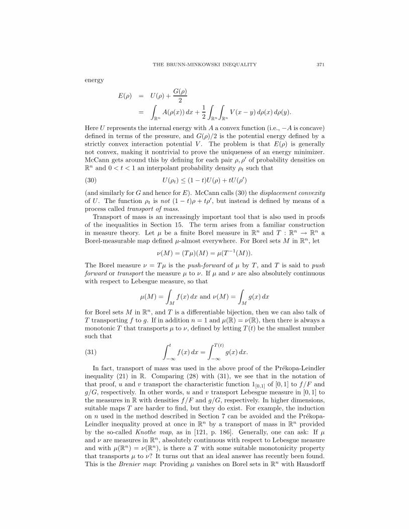
Here U represents the internal energy with A a convex function (i.e., −A is concave)defined in terms of the pressure, and G(ρ)/2 is the potential energy defined by astrictly convex interaction potential V . The problem is that E(ρ) is generallynot convex, making it nontrivial to prove the uniqueness of an energy minimizer.McCann gets around this by defining for each pair ρ, ρ′ of probability densities onRn and 0 < t < 1 an interpolant probability density ρt such that

U(ρt) ≤ (1− t)U(ρ) + tU(ρ′)(30)

(and similarly forG and hence forE). McCann calls (30) the displacement convexityof U . The function ρt is not (1 − t)ρ + tρ′, but instead is defined by means of aprocess called transport of mass.

Transport of mass is an increasingly important tool that is also used in proofsof the inequalities in Section 15. The term arises from a familiar constructionin measure theory. Let µ be a finite Borel measure in Rn and T : Rn → Rn aBorel-measurable map defined µ-almost everywhere. For Borel sets M in Rn, let

ν(M) = (Tµ)(M) = µ(T−1(M)).

The Borel measure ν = Tµ is the push-forward of µ by T , and T is said to pushforward or transport the measure µ to ν. If µ and ν are also absolutely continuouswith respect to Lebesgue measure, so that

µ(M) =∫M

f(x) dx and ν(M) =∫M

g(x) dx

for Borel sets M in Rn, and T is a differentiable bijection, then we can also talk ofT transporting f to g. If in addition n = 1 and µ(R) = ν(R), then there is always amonotonic T that transports µ to ν, defined by letting T (t) be the smallest numbersuch that ∫ t

−∞f(x) dx =

∫ T (t)

−∞g(x) dx.(31)

In fact, transport of mass was used in the above proof of the Prekopa-Leindlerinequality (21) in R. Comparing (28) with (31), we see that in the notation ofthat proof, u and v transport the characteristic function 1[0,1] of [0, 1] to f/F andg/G, respectively. In other words, u and v transport Lebesgue measure in [0, 1] tothe measures in R with densities f/F and g/G, respectively. In higher dimensions,suitable maps T are harder to find, but they do exist. For example, the inductionon n used in the method described in Section 7 can be avoided and the Prekopa-Leindler inequality proved at once in Rn by a transport of mass in Rn providedby the so-called Knothe map, as in [121, p. 186]. Generally, one can ask: If µand ν are measures in Rn, absolutely continuous with respect to Lebesgue measureand with µ(Rn) = ν(Rn), is there a T with some suitable monotonicity propertythat transports µ to ν? It turns out that an ideal answer has recently been found.This is the Brenier map: Providing µ vanishes on Borel sets in Rn with Hausdorff

372 R. J. GARDNER

dimension n− 1, there is a convex function ψ : Rn → R such that if T = ∇ψ, thenT transports µ to ν. See [16] for more details and references.

McCann’s definition of the probability density ρt in (30) uses the Brenier map.If ψ is such that ∇ψ transports ρ to ρ′, then ρt is the result of transporting ρ bythe map (1− t)In + t∇ψ, where In is the identity map on Rn.

McCann [114], [115] exploits the Brenier map as a localization technique toderive new global convexity inequalities which imply the Brunn-Minkowski andPrekopa-Leindler inequalities as special cases. In particular, he is able to recoverthe Brunn-Minkowski inequality from (30) by taking A(ρ) = −ρ(n−1)/n and ρ andρ′ to be the densities corresponding to the uniform probability measures in the twosets.

9. p-Concave and log-concave functions, and diffusion equations

A nonnegative function f on Rn is called p-concave on a convex set C if

f ((1− λ)x + λy) ≥Mp(f(x), f(y), λ),

for all x, y ∈ C and 0 < λ < 1, where the right-hand side is the p-mean defined asin Section 7. Note that if p > 0, then f is p-concave if and only if fp is concave, andin particular, 1-concave is just concave in the usual sense. If p = 0, the previousinequality reads

f ((1− λ)x + λy) ≥ f(x)1−λf(y)λ,(32)

which is equivalent to saying that log f is concave on C. In this case, therefore, theconvention is to call f log concave instead. It follows from Jensen’s inequality (23)that a p-concave function is q-concave for all q ≤ p.

If f and g are log concave on C and D, respectively, then h(x, y) = f(x)g(y) isclearly log concave on C×D. In view of its hypothesis (20), it is not surprising thatthe Prekopa-Leindler inequality (21) has much to say about log-concave functions.For example, suppose that f is an integrable log-concave function on an open convexset C in Rm+n, and for each x in the orthogonal projection C|Rm of C onto Rmwe let C(x) = y ∈ Rn : (x, y) ∈ C and define

F (x) =∫C(x)

f(x, y) dy.

The Prekopa-Leindler inequality quickly implies that F , sometimes called a sectionof f , is also log concave on C|Rm. To see this, let xi ∈ C|Rm and gi(y) = f(xi, y)for y ∈ C(xi), i = 0, 1. Suppose that 0 < λ < 1 and that x = (1− λ)x0 + λx1, andlet g(y) = f(x, y) for y ∈ C(x). If yi ∈ C(xi), i = 0, 1, and y = (1−λ)y0 +λy1, thenthe log concavity of f implies that g ((1 − λ)y0 + λy1) ≥ g0(y0)1−λg1(y1)λ. Also,C(x) ⊃ (1− λ)C(x0) + λC(x1), from which it follows that

g(y)1C(x)(y) ≥(g0(y0)1C(x0)(y0)

)1−λ (g1(y1)1C(x1)(y1)

)λ.

Comparing with (20), we can apply the Prekopa-Leindler inequality (21) to obtain

F ((1 − λ)x0 + λx1) = F (x) =∫Rnf(x, y)1C(x)(y) dy

≥(∫

Rnf(x0, y0)1C(x0)(y0) dy0

)1−λ(∫Rnf(x1, y1)1C(x1)(y1) dy1

)λ= F (x0)1−λF (x1)λ,

as required.


Recall that

(f ∗ g)(x) =∫Rnf(x− y)g(y) dy(33)

is the convolution of measurable functions f and g on Rn. Suppose that f and g arelog concave on open convex sets C and D, respectively, in Rn. Then f(x − y)g(y)is log concave for (x − y, y) ∈ C ×D, that is, for x ∈ C +D. The log concavity ofsections of log-concave functions now implies that f ∗ g is log concave on C + D.In short, the convolution of log-concave functions is log concave. This fact findsuses in probability theory (see Section 11). For now, an application to diffusionequations will be sketched.

Let V be a nonnegative continuous potential defined on a convex domain C inRn and consider the diffusion equation

∂ψ

∂t=

124ψ − V (x)ψ(x, t)(34)

with zero Dirichlet boundary condition (i.e., ψ tends to zero as x approaches theboundary of C for each fixed t). Denote by f(x, y, t) the fundamental solution of(34); that is, ψ(x, t) = f(x, y, t) satisfies (34) and its boundary condition, and

limt→0+

f(x, y, t) = δ(x − y),

where δ is the Dirac δ-function. For example, if V = 0 and C = Rn, one can showthat

f(x, y, t) = (2πt)−n/2e−|x−y|2/2t,

which is log concave on C2 for each t. Brascamp and Lieb [34] used the Prekopa-Leindler inequality (21) to show that f(x, y, t) is actually log concave on C2 when-ever V is convex. Basically, it is shown that f is given as a pointwise limit ofconvolutions of log-concave functions, and these convolutions, as we now know, arelog concave. Borell [29] uses a version of Theorem 10.1 to show that the strongerassumption that V is −1/2-concave implies that t log(tnf(x, y, t2)) is concave onC2 × R+.

In a further study, Borell [31] generalizes all of these results (and the Prekopa-Leindler inequality) by considering potentials V (σ, x) that depend also on a pa-rameter σ. This work yields a “Brownian motion” proof of the Brunn-Minkowskiinequality.

McCann’s displacement convexity (30) plays an essential role in recent work ofOtto [125], who observed that various diffusion equations can be viewed as gradientflows in the space of probability measures with the Wasserstein metric (formally, atleast, an infinite-dimensional Riemannian structure). McCann’s interpolation usingthe Brenier map gives the geodesics in this space, and Otto uses the displacementconvexity to derive rates of convergence to equilibrium.

10. The Borell-Brascamp-Lieb inequality and other extensions

Figure 1 shows several far-reaching generalizations of the Brunn-Minkowski andPrekopa-Leindler inequalities that will be discussed later. This section will addresssome others that lie closer to (10) and (21).

Firstly, there are convenient forms of these inequalities that avoid measurabilityassumptions. The assumption in the general Brunn-Minkowski inequality (10) that

374 R. J. GARDNER

the set (1−λ)X+λY is measurable is necessary, since an old example of Sierpinski[138] shows that this set may not be measurable even whenX and Y are measurable.There are a couple of ways around this. One can simply replace the measure onthe left of (10) by inner Lebesgue measure V∗n, the supremum of the measures ofcompact subsets, thus:

V∗n ((1 − λ)X + λY )1/n ≥ (1 − λ)Vn(X)1/n + λVn(Y )1/n.

A better solution is to obtain a slightly improved version of the Prekopa-Leindlerinequality, and then deduce a corresponding improved Brunn-Minkowski inequality,as follows.

Recall that the essential supremum of a measurable function f on Rn is definedby

ess supx∈Rn

f(x) = inft : f(x) ≤ t for almost all x ∈ Rn.

Brascamp and Lieb [34] proved the following essential form of the Prekopa-Leindler inequality. (According to Uhrin [147], the idea of using the essentialsupremum in connection with our topic occurred independently to S. Dancs.) Let0 < λ < 1 and let f, g ∈ L1(Rn) be nonnegative. Let

s(x) = ess supyf

(x− y1− λ

)1−λg( yλ

)λ.(35)

Then s is measurable and∫Rns(x) dx ≥

(∫Rnf(x) dx

)1−λ (∫Rng(x) dx

)λ.(36)

For the proof, the measurability of s is first established by observing that

s(x) = supφ∈D

∫Rnf

(x− y1− λ

)1−λg( yλ

)λφ(y) dy,

where D is a countable dense subset of the unit ball of L1(Rn). Therefore s is thesupremum of a countable family of measurable functions. With the measurabilityof s in hand, the proof of (36) follows that of the usual Prekopa-Leindler inequalityoutlined in Section 7.

The essential form (36) of the Prekopa-Leindler inequality implies the usual form(21). To see this, replace x by z and y by λy′ in (35) and then let x = (z−λy′)/(1−λ)to obtain

s(z) = ess supy′f

(z − λy′1− λ

)1−λg(y′)λ

= ess supf(x)1−λg(y)λ : z = (1− λ)x + λy.Now if h is any integrable function satisfying

h ((1− λ)x + λy) ≥ f(x)1−λg(y)λ,

then h ≥ s almost everywhere and (21) follows directly.The corresponding improvement of the Brunn-Minkowski inequality requires one

new concept. Note that the usual vector sum of X and Y can be written

X + Y = z : X ∩ (z − Y ) 6= ∅.Adjust this by defining the essential sum of X and Y by

X +e Y = z : Vn (X ∩ (z − Y )) > 0.


The essential form of the Brunn-Minkowski inequality states that if 0 < λ < 1 andX and Y are nonempty bounded measurable sets in Rn, then

Vn ((1− λ)X +e λY )1/n ≥ (1 − λ)Vn(X)1/n + λVn(Y )1/n.(37)

A direct proof of this result is given in [34, Appendix]. It is not difficult to deriveit from (36), as in [63, Theorem 9.2].

The following theorem, the Borell-Brascamp-Lieb inequality, uses the p-meansMp introduced in Section 7 to generalize the Prekopa-Leindler inequality, which isjust the case p = 0. The number p/(np+ 1) is interpreted in the obvious way; it isequal to −∞ when p = −1/n and to 1/n when p =∞.

Theorem 10.1. Let 0 < λ < 1, let −1/n ≤ p ≤ ∞, and let f , g, and h benonnegative integrable functions on Rn satisfying

h ((1− λ)x+ λy) ≥Mp (f(x), g(y), λ) ,

for all x, y ∈ Rn. Then∫Rnh(x) dx ≥Mp/(np+1)

(∫Rnf(x) dx,

∫Rng(x) dx, λ

).(38)

This result has some significant consequences in probability theory that are dis-cussed in the next section. With a single technical lemma concerning p-means inhand, Theorem 10.1 can be proved by essentially the same argument given in Sec-tion 7 for the proof of Theorem 7.1; see [63, Section 10] for the details. The resultwas first proved (in slightly modified form) for p > 0 by Henstock and Macbeath[77] (when n = 1) and Dinghas [49]. The limiting case p = 0 was also provedby Prekopa and Leindler, as noted above, and rediscovered by Brascamp and Lieb[32]. In general form Theorem 10.1 is stated and proved by Brascamp and Lieb [34,Theorem 3.3] and by Borell [27, Theorem 3.1] (but with a much more complicatedproof; see also the paper of Rinott [131]). The method of proof just indicated isemployed in [43] and [46] (see also [48, Theorem 3.15]), but still draws on methodsintroduced by Henstock, Macbeath, and Dinghas. Das Gupta’s survey [46] con-tains a very thorough examination and assessment of the various contributions andproofs before 1980. Brascamp and Lieb [34] obtain an “essential” form of Theo-rem 10.1, as in the case p = 0 (see (36)). Dancs and Uhrin [43] also offer a versionof Theorem 10.1 for −∞ ≤ p < −1/n.

In calling Theorem 10.1 the Borell-Brascamp-Lieb inequality we are followingthe authors of [41] (who also generalize it to a Riemannian manifold setting; seeSection 12) and placing the emphasis on the negative values of p. In fact, it can beshown (see [41] and [63, Section 10]) that Theorem 10.1 for p = −1/n implies The-orem 10.1 for all p > −1/n. The approach of Brascamp and Lieb [34], incidentally,was to observe that Theorem 10.1 also holds for n = 1 and p = −∞, and then toderive Theorem 10.1 for n = 1 and p ≥ −1 from this and the technical lemma forp-means mentioned earlier.

An interesting sharpening of the Brunn-Minkowski inequality was found by Bon-nesen in 1929 (see [43]). If X is a bounded measurable set in Rn, the inner sectionfunction mX of X is defined by

mX(u) = supt∈R

Vn−1

(X ∩ (u⊥ + tu)

),

for u ∈ Sn−1. (In 1926, Bonnesen asked if this function determines a convex bodyin Rn, n ≥ 3, up to translation and reflection in the origin, a question that remains

376 R. J. GARDNER

unanswered; see [66, Problem 8.10]). Bonnesen proved that if 0 < λ < 1 andu ∈ Sn−1, then

Vn ((1 − λ)X + λY ) ≥M1/(n−1) (mX(u),mY (u), λ)(

(1− λ)Vn(X)mX(u)

+ λVn(Y )mY (u)

).

(39)

It is not hard to show that this is indeed stronger than (10). As Dancs and Uhrin[43, Theorem 3.2] show, an integral version of (39), in a general form similar toTheorem 10.1, can be constructed from the ideas already presented here.

At present, the most general results in Euclidean space of the type considered inthis section are contained in the papers of Uhrin; see [147], [148], and the referencesgiven there. In particular, Uhrin states in [148, p. 306] that all previous resultsof this sort are contained in [148, (3.42)]. The latter inequality has as ingredientstwo kinds of curvilinear convex combinations of vectors, and its proof reintroducesgeometrical methods.

11. Applications to probability and statistics

In 1955, Anderson [2] used the Brunn-Minkowski inequality in his work on mul-tivariate unimodality. He began with the following simple observation. If a nonneg-ative integrable function f on R is (i) symmetric (f(x) = f(−x)) and (ii) unimodal(f(cx) ≥ f(x) for 0 ≤ c ≤ 1), and I is an interval centered at the origin, then∫

I+y

f(x) dx

is maximized when y = 0. In probability language, if a random variable X hasprobability density f and Y is an independent random variable, then

ProbX ∈ I ≥ ProbX + Y ∈ I.

To see this, recall that if X and Y are independent random vectors on Rn with prob-ability densities f and g, respectively, then f ∗g (defined by (33)) is the probabilitydensity of X + Y ; see, for example, [82, Section 11.5]. So, by Fubini’s theorem,

ProbX + Y ∈ I =∫I

∫Rf(z − y)g(y) dy dz =

∫R

∫I

f(z − y)g(y) dz dy

=∫R

∫I−y

f(x)g(y) dx dy ≤∫R

∫I

f(x)g(y) dx dy

=∫I

f(x) dx = ProbX ∈ I.

The next result, Anderson’s theorem, is a generalization of this that applies tounimodal functions f on Rn, those whose level sets L(f, t) (see (29)) are convex foreach t ≥ 0.

Theorem 11.1. Let K be an origin-symmetric convex body in Rn and let f be anonnegative, symmetric, and unimodal function integrable on Rn. Then∫

K

f(x+ cy) dx ≥∫K

f(x+ y) dx,

for 0 ≤ c ≤ 1 and y ∈ Rn.


This says that the integral of a symmetric unimodal function f over an n-dimensional centrally symmetric convex body K does not decrease when K istranslated towards the origin. Since the graph of f forms a hill whose peak isover the origin, this is intuitively clear. However, it is no longer obvious, as it wasin the 1-dimensional case! There may be points x ∈ K at which the value of f islarger than it is at the corresponding translate of x.

As above, we can conclude from Anderson’s theorem that if a random variableX has probability density f on Rn and Y is an independent random variable, then

Prob X ∈ K ≥ ProbX + Y ∈ K,

where K is any origin-symmetric convex body in Rn.The proof of Anderson’s theorem hinges on a property of a function gK,L on Rn

associated with convex bodies K and L in Rn, defined by

gK,L(x) = V (K ∩ (L + x)) .

The Brunn-Minkowski inequality (2) can be used to show that gK,L is 1/n-concaveon its support (see [63, Theorem 13.1]), but its log concavity is all that is requiredfor Anderson’s theorem. This follows from observing that gK,L is a convolution ofcharacteristic functions, since

gK,L(x) =∫Rn

1K∩(L+x)(y) dy =∫Rn

1K(y)1L+x(y) dy

=∫Rn

1K(y)1L(y − x) dy = (1−L ∗ 1K)(x).

It was proved in Section 9 that the convolution of log-concave functions is logconcave, and it follows that gK,L is log concave on its support. Of course, thePrekopa-Leindler inequality (21) has been at work behind the scenes.

The relevance of gK,L to Anderson’s theorem comes from taking f(x) = 1L(x),where 1L is the characteristic function of an origin-symmetric convex body L inRn. Then f(x+ y) = 1L(x+ y) = 1L−y(x) and∫

K

f(x+ y) dx =∫K

1L−y(x) dx = V (K ∩ (L− y)) = gK,L(−y) = gK,L(y).

The log concavity of gK,L allows one to conclude that gK,L(cy) ≥ gK,L(y) for0 ≤ c ≤ 1 (see [63, Theorem 13.1] for the details), and the theorem follows for thisspecial case. The general case results from applying this special case to the origin-symmetric convex bodies L = L(f, t) formed by the level sets of f , and integratingover t ≥ 0.

The function gK = gK,K associated with a single convex body K in Rn, andgiving the volumes of its intersection with its translates, is called the covariogramofK and is of considerable interest in its own right. The name stems from the theoryof random sets, where the covariance is defined for x ∈ Rn as the probability thatboth o and x lie in the random set. The covariogram is also useful in mathematicalmorphology; see [136, Chapter 9]) and [141, Section 6.2]. In 1986, G. Matheron(see the references in [133]) asked if the covariogram determines convex bodies, upto translation and reflection in the origin. Remarkably, this question is open forn = 2! Bianchi [22] has shown that the answer is affirmative for a large class ofplanar convex bodies. He has also found pairs of convex polyhedra that representcounterexamples in R4.

378 R. J. GARDNER

Anderson’s theorem has many applications in probability and statistics, where,for example, it can be applied to show that certain statistical tests are unbiased. See[2], [35], [48], and [145]. Certain of these applications are also associated with thePrekopa-Leindler inequality (21) and its generalization, the Borell-Brascamp-Liebinequality (38).

In Section 9 it was shown that the Prekopa-Leindler inequality yields the logconcavity of certain functions. It can also provide the log concavity of measures.Suppose that f is a nonnegative integrable function defined on a measurable subsetC of Rn, and µ is defined by

µ(X) =∫C∩X

f(x) dx,

for all measurable subsets X of Rn. Then we say that µ is generated by f andC. With an argument similar to that in Section 9 showing that sections of a log-concave function are log concave, the Prekopa-Leindler inequality (21) implies thatif f is log concave and C is an open convex subset of its support, then the measureµ generated by f and C is also log concave in the sense that

µ ((1− λ)X + λY ) ≥ µ(X)1−λµ(Y )λ,

for all measurable sets X and Y in Rn and 0 < λ < 1. The details can be found in[63, Section 10].

Prekopa [128], [130, Chapter 8] explains the applications of this result, and thosein Section 9 on log-concave functions, to stochastic programming. It can be seen inaction, however, when applied to the multivariate normal distribution on Rn withmean m ∈ Rn and n×n positive definite symmetric covariance matrix A. This hasprobability density

f(x) = c exp(− (x−m) ·A−1(x−m)

2

),

where c = (2π)−n/2(detA)−1/2. Since A is positive definite, the function −(x−m) ·A−1(x−m) is concave and so f is log concave. It follows that the measure generatedby f is also log concave. The same conclusion can be drawn for other importantdistributions, such as the Wishart, multivariate β, and Dirichlet distributions; see[128].

The Borell-Brascamp-Lieb inequality (38) provides concavity properties of sec-tions and convolutions of functions, just as its special case p = 0, the Prekopa-Leindler inequality (21), does (see Section 9). Details can be found in [63, Sec-tion 11]. Concavity properties of measures can also be obtained. A finite (non-negative) measure µ defined on (Lebesgue) measurable subsets of Rn is p-concaveif

µ ((1− λ)X + λY ) ≥Mp(µ(X), µ(Y ), λ),

for all measurable sets X and Y in Rn and 0 < λ < 1. Then a 0-concave measure islog concave, and it follows from Jensen’s inequality (23) that a p-concave measureis q-concave for all q ≤ p. Theorem 10.1 and an argument similar to that for thelog-concave case yield the following corollary.

Corollary 11.2. Let −1/n ≤ p ≤ ∞ and let f be an integrable p-concave functionon a convex set C in Rn. Then the measure generated by f and C is p/(np+ 1)-concave.


See [63, Corollary 10.3] or [48, Theorem 3.16]. Much of the book [48] is de-voted to such results and their applications to probability. The extra generalitymay seem superfluous, but even the negative values of p are useful. For example,Borell [27] noted that the density functions of the multivariate Pareto (the Cauchydistribution is a special case), t, and F distributions are not log concave, but are p-concave for some p < 0, and the more general result furnishes concavity propertiesof corresponding probability measures.

The general Brunn-Minkowski inequality (10) says that Lebesgue measure in Rnis 1/n-concave, and Theorem 10.1 supplies plenty of measures that are p-concavefor −1/n ≤ p ≤ ∞. Borell [27] (see also [48, Theorem 3.17]) proves a sort ofconverse to Corollary 11.2: Given −∞ ≤ p ≤ 1/n and a p-concave measure µ withn-dimensional support S, there is a p/(1−np)-concave function on S that generatesµ. Borell also observed that when p > 1/n, no nontrivial p-concave measures existin Rn, and that any 1/n-concave measure is a multiple of Lebesgue measure; see[48, Theorem 3.14]. Dancs and Uhrin [43, Theorem 3.4] find a generalization ofTheorem 10.1 in which Lebesgue measure is replaced by a q-concave measure forsome −∞ ≤ q ≤ 1/n.

Corollary 11.2 and Anderson’s theorem are related. If K is a convex body in Rn,y ∈ Rn, p ≥ −1/n, and f is an integrable p-concave function on Rn, Corollary 11.2can be used to show that the function

h(y) =∫K

f(x+ y) dx

is p/(np + 1)-concave on Rn and hence unimodal. (See [63, Section 13] for thedetails.) In particular, h(cy) is unimodal in c for a fixed y, as in the conclusion ofTheorem 11.1. Anderson’s theorem replaces the restriction that f is p-concave forp ≥ −1/n with a much weaker condition, but requires in exchange the symmetryof f and K.

12. Brunn-Minkowski and Prekopa-Leindler in other spaces

Like the isoperimetric inequality, the inequalities met in previous sections haveversions that hold in other spaces. These versions also act as portals to activeresearch areas already detailed in separate surveys. Naturally, it is only possiblehere to touch on these captivating topics.

Let X be a measurable subset of Rn and let rX be the radius of a ball of thesame volume as X . If ε > 0, the general Brunn-Minkowski inequality (11) impliesthat

Vn(X + εB) ≥(Vn(X)1/n + εVn(B)1/n

)n=(Vn(rXB)1/n + εVn(B)1/n

)n= Vn(rXB + εB).

(40)

For any set A, let

Aε = A+ εB = x : d(x,A) ≤ ε.(41)

Then we can rewrite (40) as

Vn(Xε) ≥ Vn((rXB)ε).(42)

Notice that (42), by virtue of (41), is now free of the addition and involves only ameasure and a metric.

380 R. J. GARDNER

With the appropriate measure and metric replacing Vn and the Euclidean metric,(42) remains true in the sphere Sn−1 and hyperbolic space, equality holding if andonly if X is a ball. (Of course, in these spaces, the ball centered at x and with radiusr > 0 is the set of all points whose distance from x is at most r. In Sn−1, ballsare just spherical caps.) Though in Rn (42) is only a special case of (11), in Sn−1

and hyperbolic space, (42) is called the Brunn-Minkowski inequality. Accordingto Dudley [51, p. 184], (42) was first proved in Sn−1 under extra assumptions byP. Levy in 1922, with weaker assumptions by E. Schmidt in the 1940’s, and in fullgenerality by Figiel, Lindenstrauss, and Milman in 1977. In hyperbolic space, (42)is due to E. Schmidt. A proof using symmetrization techniques for both Sn−1 andhyperbolic space can be found in [36, Section 9].

Perhaps more significant than (42) for recent developments is a surprising resultthat holds in Sn−1, n ≥ 3, with the chordal metric (i.e., the metric inheritedfrom the Euclidean distance in Rn). It can be shown that if X ⊂ Sn−1 andVn−1(X)/Vn−1(Sn−1) ≥ 1/2 and 0 < ε < 1, then

Vn−1(Xε)Vn−1(Sn−1)

≥ 1−(π

8

)1/2

e−(n−2)ε2/2.(43)

This inequality, which again goes back to P. Levy, is proved in [121, p. 5]. Resultsof the form (43) are called approximate isoperimetric inequalities, and can be de-rived from the general Brunn-Minkowski inequality (10), as in [4, Theorem 2]. Inparticular, by taking X to be a hemisphere, we see that for large n, almost all themeasure is concentrated near the equator! This is an example of the concentrationof measure phenomenon that Milman applied in his 1971 proof of Dvoretzky’s theo-rem and that with contributions by Talagrand and others has quickly generated anextensive literature surveyed by Ledoux [85], [86]. An excellent, but more selective,introduction is Ball’s elegant and insightful expository article [12, Lecture 8].

Analogous results hold in Gauss space, Rn with the usual metric but with thestandard Gauss measure γn in Rn with density

dγn(x) = (2π)−n/2e−‖x‖2/2 dx.(44)

Indeed, for bounded Lebesgue measurable sets X and Y in Rn for which (1−λ)X+λY is Lebesgue measurable, there is the inequality

γn((1− λ)X + λY ) ≥ γn(X)1−λγn(Y )λ(45)

corresponding to (22). This follows from the Prekopa-Leindler inequality (21) (be-cause the density function is log concave); see, for example, [32]. It can also bederived directly from the general Brunn-Minkowski inequality (10) by means ofthe “Poincare limit”, a limit of projections of Lebesgue measure in balls of in-creasing radius; this and an abundance of additional information and referencescan be found in Ledoux and Talagrand’s book [87, Section 1.1]. To describe someof this work briefly, let Φ(r) = γ1((−∞, r)) for r ∈ R. Borell [26] and Sudakovand Tsirel’son [142] independently showed that if X is a measurable subset of Rnand γn(X) = Φ(rX), then γn(Xε) ≥ Φ(rX + ε), with equality if X is a half-space.Ehrhard [53], [54] gave a new proof using symmetrization techniques that also yieldsthe following Brunn-Minkowski-type inequality: If K and L are convex bodies inRn and 0 < λ < 1, then

Φ−1 (γn((1 − λ)K + λL)) ≥ (1− λ)Φ−1 (γn(K)) + λΦ−1 (γn(L)) .(46)


While (46) is stronger than (45) for convex bodies, it is unknown whether it holdsfor Borel sets; see [84] and [87, Problem 1]. An approximate isoperimetric inequalitysimilar to (43) also holds in Gauss space; Maurey [113] (see also [12, Theorem 8.1])found a simple proof employing the Prekopa-Leindler inequality (21). As in Sn−1,there is a concentration of measure in Gauss space, this time in spherical shells ofthickness approximately 1 and radius approximately

√n. Closely related work on

logarithmic Sobolev inequalities is outlined in Section 14.Borell [30] applies his Brunn-Minkowski inequality in Gauss space to option

pricing, assuming that underlying stock prices are governed by a joint Brownianmotion.

Bahn and Ehrlich [5] find an inequality that can be interpreted as a reversedform of the Brunn-Minkowski inequality in Minkowski spacetime, that is, Rn+1

with a scalar product of index 1.Cordero-Erausquin [40] utilizes results of McCann to prove a version of the

Prekopa-Leindler inequality on the sphere, remarking that a similar version canbe obtained for hyperbolic space. These results are generalized in a remarkablepaper [41] by Cordero-Erausquin, McCann, and Schmuckenschlager, who establisha beautiful Riemannian version of Theorem 10.1.

13. Young’s inequality

Convolutions have already been featured in this story, in Sections 9 and 11.By 1976, it was known that a sharp convolution inequality actually implies theBrunn-Minkowski inequality. This sharp convolution inequality is a refinement ofan earlier one with roots in Fourier analysis. The classical Young inequality statesthat if p, q, r ≥ 1,

1p

+1q

= 1 +1r,(47)

and f ∈ Lp(Rn) and g ∈ Lq(Rn) are nonnegative, then

‖f ∗ g‖r ≤ ‖f‖p‖g‖q.(48)

This was proved by W. H. Young around 1912 (see [76, Sections 8.3 and 8.4] andthe references given there); a few lines and Holder’s inequality (25) suffice, as in[91, p. 99].

The next theorem provides two convolution inequalities with sharp constants,the first a sharp form of (48) proved independently by Beckner [20] and Brascampand Lieb [33], and the second a reverse form found by Brascamp and Lieb [33](refining an earlier version due to Leindler [88]).

Theorem 13.1. Let 0 < p, q, r satisfy (47), and let f ∈ Lp(Rn) and g ∈ Lq(Rn)be nonnegative. Then(Young’s inequality)

‖f ∗ g‖r ≤ Cn‖f‖p‖g‖q, for p, q, r ≥ 1,(49)

and(Reverse Young inequality)

‖f ∗ g‖r ≥ Cn‖f‖p‖g‖q, for p, q, r ≤ 1.(50)

382 R. J. GARDNER

Here C = CpCq/Cr, where

C2s =

|s|1/s|s′|1/s′(51)

for 1/s+ 1/s′ = 1 (i.e., s and s′ are Holder conjugates).

The inequality (49), when expanded, reads as follows:(∫Rn

(∫Rnf(x− y)g(y) dy

)rdx

)1/r

≤ Cn(∫

Rnf(x)p dx

)1/p(∫Rng(x)q dx

)1/q

.

Inequalities (49) and (50) together show that equality holds in both when p = q =r = 1. In fact, since Cp → 1 as p → 1, when p = q = r = 1 we have C = 1; andsubstituting u = x − y, v = y in the left-hand side of (49) and (50), we see thatthis case reduces to the familiar equation∫

Rn

∫Rnf(u)g(v) dv du =

∫Rnf(x) dx

∫Rng(x) dx.

The relevance of these convolution inequalities stems from Brascamp and Lieb’sremarkable discovery that the limiting case r → 0 of the reverse Young inequality(50) is the essential form (36) of the Prekopa-Leindler inequality. The clever proofcan be found in [33] (or see [63, Theorem 14.2]). One first observes that it suffices toprove (36) when f and g are bounded measurable functions with compact support.If the function s is defined by (35), then it can be shown that∫

Rns(x) dx = lim

m→∞

∫Rn

(∫Rnf

(x− y1− λ

)(1−λ)m

g( yλ

)λmdy

)1/(m−1)

dx.

(If we replaced the exponent 1/(m−1) by 1/m, this would follow from the fact thatthe mth integral mean tends to the supremum as m → ∞; compare [76, p. 143].But this replacement is irrelevant in the limit.) Now (36) results from applying thereverse Young inequality (50) with m > max(1 − λ)−1, λ−1, p = 1/((1 − λ)m),q = 1/(λm), and r = 1/(m− 1). This sketch is somewhat unsatisfying, of course,since one has to complete all the computations to see how the constant Cn in (50)magically evaporates in the limit.

Even the simplest known proofs of (49) or (50), due to Barthe [17], necessarilyalso require a considerable amount of computation. It is worth mentioning, how-ever, that the method includes both the parametrization technique and inductionon dimension employed in Section 7 for proving the Prekopa-Leindler inequality.Barthe’s ingenious proof supplies (49) and (50) at once, together with the followingequality condition, originally established by Brascamp and Lieb [33]: When n = 1and p, q 6= 1, equality holds in (49) or (50) if and only if f and g are Gaussians:

f(x) = ae−c|p′|(x−α)2

, g(x) = be−c|q′|(x−β)2

,

for some a, b, c, α, β with a, b ≥ 0 and c > 0.The classical Young inequality (48) was motivated by the classical Hausdorff-

Young inequality: If 1 ≤ p ≤ 2 and f ∈ Lp(Rn), then

‖f‖p′ ≤ ‖f‖p,(52)


where f denotes the Fourier transform

f(x) =∫Rnf(y)e2πix·y dy

of f , and p and p′ are Holder conjugates. This was proved by Hausdorff and Youngfor Fourier series, and extended to integrals by Titchmarsh in 1924. Beckner [20],improving on earlier partial results of Babenko, showed that when 1 ≤ p ≤ 2,

‖f‖p′ ≤ Cnp ‖f‖p,(53)

where Cp is given by (51). (Lieb [90] proved that equality holds only for Gaussians.)This improvement on (52) is related to Young’s inequality (49). To see the con-nection, suppose that (53) holds, n = 1, and 1 ≤ p, q, r′ ≤ 2. If p, q, r satisfy (47),then their Holder conjugates satisfy 1/p′ + 1/q′ = 1/r′. Using this and Holder’sinequality (25), we obtain

‖f ∗ g‖r ≤ Cr′‖f g‖r′≤ Cr′‖f‖p′‖g‖q′≤ Cr′(Cp‖f‖p)(Cq‖g‖q) = C‖f‖p‖g‖q.

A similarly easy argument (see [20, pp. 169–70]) shows that Young’s inequality (49)yields (52) when p′ is an even integer.

Later on the following second form of Young’s inequality will be useful. Let0 < p, q, r satisfy

1p

+1q

+1r

= 2,

and let f ∈ Lp(Rn), g ∈ Lq(Rn), and h ∈ Lr(Rn) be nonnegative. Then∫Rn

∫Rnf(x)g(x− y)h(y) dy dx ≤ Cn‖f‖p‖g‖q‖h‖r,(54)

where C = CpCqCr is defined using (51). The second form of Young’s inequality isactually equivalent to (49); see [91, p. 99] or [66, Section 13] for the proof.

14. Information theory, physics, and logarithmic Sobolev

inequalities

Young’s inequality (49) implies a famous inequality from information theorycalled the entropy power inequality. This section explains the connection andtouches on some aspects that relate to physics and logarithmic Sobolev inequal-ities.

Suppose that X is a discrete random variable taking possible values x1, . . . , xmwith probabilities p1, . . . , pm, respectively, where

∑i pi = 1. Shannon [137] intro-

duced a measure of the average uncertainty removed by revealing the value of X .This quantity,

Hm(p1, . . . , pm) = −m∑i=1

pi log pi,

is called the entropy of X . It can also be regarded as a measure of the missinginformation; indeed, the function Hm is concave and achieves its maximum whenp1 = · · · = pm = 1/m, that is, when all outcomes are equally likely. The words“uncertainty” and “information” already suggest a connection with physics, and

384 R. J. GARDNER

a derivation of the function Hm from a few natural assumptions can be found intextbooks on statistical mechanics; see, for example, [6, Chapter 3].

If X is a random vector in Rn with probability density f , the entropy h1(X) ofX is defined analogously:

h1(X) = h1(f) = −∫Rnf(x) log f(x) dx.

This notation is convenient when h1(X) is regarded as a limit as p→ 1 of the pthRenyi entropy hp(X) of X , defined for p > 1 by

hp(X) = hp(f) =p

1− p log ‖f‖p.

The entropy of X may not be well defined. However, if f ∈ L1(Rn)∩Lp(Rn) forsome p > 1, then h1(X) = h1(f) is well defined, though its value may be +∞.

The entropy power N(X) of X is

N(X) =1

2πeexp

(2nh1(X)

).

With this background, the entropy power inequality can be stated: Let X and Y beindependent random vectors in Rn with probability densities in Lp(Rn) for somep > 1. Then

N(X + Y ) ≥ N(X) +N(Y ).(55)

In 1948, Shannon [137, Theorem 15 and Appendix 6] published this inequalityand used it to obtain a lower bound [137, Theorem 18] for the capacity of a channel.Shannon’s proof shows that equality holds in (55) if X and Y are multivariatenormal with proportional covariances. In fact equality holds only for such X andY , as Stam’s different proof [139] (simplified in [23] and [47]) of (55) shows.

The most accessible direct proof of (55) seems to be that of Blachman [23]. AsLieb [89] discovered, however, the limiting case r → 1 of Young’s inequality (49)yields the entropy power inequality (55). A complete proof of this arresting factcan be found in [89] (or see [63, Section 18]), but Deane Yang noticed the followingequivalent and more intuitive approach. Let p > 1 and let X be a random vectorin Rn with probability density f ∈ Lp(Rn). Define

Np(X) =1

2πp−p

′/p‖f‖−2p′/np ,

where p′ is the Holder conjugate of p (see (51)). Then Np(X), which might becalled the pth Renyi entropy power of X , converges to N(X) as p→ 1+. Supposethat 0 < λ < 1, and for r > 1, let

p = p(r) =r

(1− λ) + λrand q = q(r) =

r

λ+ (1 − λ)r.

Then p, q > 1, and (47) is satisfied. Let X and Y be independent random vectorsin Rn with probability densities f ∈ Lp(Rn) and g ∈ Lq(Rn), respectively. Young’sinequality (49) implies that

Nr(X + Y ) ≥(Np(X)1− λ

)1−λ(Nq(Y )λ

)λ.(56)


(The computations required are tedious but routine.) As r → 1+, p, q → 1 and(56) becomes

N(X + Y ) ≥(N(X)1 − λ

)1−λ (N(Y )λ

)λ.(57)

By differentiating the log of the right-hand side, it can be verified that this is amaximum when λ = N(X)/(N(X) +N(Y )). Substituting this value into (57), weobtain (55).

Presumably Lieb, via his papers [33] and [89], first saw the connection betweenthe entropy power inequality (55) and the general Brunn-Minkowski inequality (10),the former being a limiting case of Young’s inequality (49) as r → 1 and the lattera limiting case of the reverse Young inequality (50) as r → 0. Later, Costa andCover [42] specifically drew attention to the analogy between the two inequalities,apparently unaware of the work of Brascamp and Lieb. The paper [73] and furtherexciting work of Lutwak, Yang, and Zhang [106], [109] reinforce this fascinatingbridge between information theory and convex geometry.

An important concept called Fisher information was employed by Stam [139] inhis proof of (55). Named after the statistician R. A. Fisher, Fisher information isclaimed in a recent book [62] by Frieden to be at the heart of a unifying principlefor all of physics! If X is a random variable with probability density f on R, theFisher information I(X) of X is

I(X) = I(f) = −∫Rf(x)(log f(x))′′ dx =

∫R

f ′(x)2

f(x)dx,

assuming these integrals exist. The multivariable form of I is a matrix, the naturalextension of this definition. The quantity I is another measure of the “sharpness”of f or the missing information in X ; see [62, Section 1.3] for a comparison of Iand h1. Stam [139] (see also [47]) showed that I can be used to obtain the Weyl-Heisenberg uncertainty inequality, and this inspired Frieden’s work. Frieden’s ideais that for any physical system, I represents how much information can possibly beobtained by measurements, while another quantity, J , is the amount of informationbound up in the system. Then I − J leads to a Lagrangian, and the correspondinglaw of physics arises from its minimization, the second derivative usually presentin such a law arising from the first derivative present in I.

Needless to say, Frieden’s claim has stirred some controversy. Some opinions canbe found in [81] and in the Mathematical Reviews review.

A complex system of inequalities swirls like a cyclone around these concepts.For example, Dembo, Cover, and Thomas [47] explore several related inequalitiesinvolving entropy, Fisher information, and uncertainty principles. Another richarea surrounds the logarithmic Sobolev inequality proved by Gross [72]:

Entγn(f) ≤ 12Iγn(f),(58)

where f is a suitably smooth nonnegative function on Rn, γn is the Gauss measurein Rn defined by (44),

Entγn(f) =∫Rnf(x) log f(x) dγn(x) −

(∫Rnf(x) dγn(x)

)(∫Rn

log f(x) dγn(x)),

386 R. J. GARDNER

and

Iγn(f) =∫Rn

‖∇f(x)‖2f(x)

dγn(x).

Here Entγn(f) and Iγn(f) are essentially the negative entropy −h1(f) and Fisherinformation, respectively, of f , defined with respect to Gauss measure. There areseveral variants of (58), some discovered earlier. An excellent introduction to suchinequalities is provided by Lieb and Loss [91, Chapter 8], where it is shown thatthey can be deduced from Young’s inequality (49) and used to estimate solutions ofthe heat equation. Bobkov and Ledoux [24] derive (58) from the Prekopa-Leindlerinequality (the “Brascamp-Lieb” in the title of [24] refers not to (59) below but to adifferent inequality of Brascamp and Lieb proved in [34]). Cordero-Erausquin [39]proves (58) directly using the transport of mass idea from Section 8.

McCann’s displacement convexity (30) is utilized by Otto and Villani [126], whofind a new proof of an inequality of Talagrand for the Wasserstein distance betweentwo probability measures in an n-dimensional Riemannian manifold, and show thatTalagrand’s inequality is very closely related to the logarithmic Sobolev inequality(58). The interested reader may also consult Ledoux’s survey [85].

15. The Brascamp-Lieb inequality and Barthe’s inequality

The inequalities presented in this section approach the most general known inthe direction of Young’s inequality and its reverse form and represent a researchfrontier that can be expected to move before too long.

Each m × n matrix A defines a linear transformation from Rn to Rm, and thislinear map can also be denoted by A. The Euclidean adjoint A∗ of A is then ann×m matrix or linear transformation from Rm to Rn satisfying Ax · y = x · A∗yfor each y ∈ Rm and x ∈ Rn.

Theorem 15.1. Let ci > 0 and ni ∈ N, i = 1, . . . ,m, with∑i cini = n. Let fi ∈

L1(Rni) be nonnegative and let Bi : Rn → Rni be a linear surjection, i = 1, . . . ,m.Then(Brascamp-Lieb inequality)∫

Rn

m∏i=1

fi(Bix)ci dx ≤ D−1/2m∏i=1

(∫Rni

fi(x) dx)ci

(59)

and(Barthe’s inequality)

∫Rn

sup

m∏i=1

fi(zi)ci : x =∑i

ciB∗i zi, zi ∈ Rni

dx ≥ D1/2

m∏i=1

(∫Rni

fi(x) dx)ci

,

(60)

where

D = inf

det (∑m

i=1 ciB∗iAiBi)∏m

i=1(detAi)ci: Ai is a positive definite ni × ni matrix

.

(61)

Theorem 15.1 is a bit intimidating at first sight! We can begin to understand ita little by taking in (59) ni = n, Bi = In, the identity map on Rn, replacing fi byf

1/cii , and letting ci = 1/pi, i = 1, . . . ,m. Then

∑i 1/pi = 1 and the log concavity


of the determinant of a positive definite matrix (see, for example, [19, p. 63]) yieldsD = 1. Therefore ∫

Rn

m∏i=1

fi(x) dx ≤m∏i=1

‖fi‖pi ,

which is just Holder’s inequality (25).Next, take m = 2, n1 = n2 = n, B1 = B2 = In, c1 = 1− λ, and c2 = λ in (60).

Again we have D = 1, so∫Rn

supf1(z1)1−λf2(z2)λ : x = (1− λ)z1 + λz2

dx

≥(∫

Rnf1(x) dx

)1−λ(∫Rnf2(x) dx

)λ,

the Prekopa-Leindler inequality (26).The true power of Theorem 15.1 begins to emerge when we see that the Brascamp-

Lieb inequality (59) implies Young’s inequality. In (59), take m = 3, n1 = n2 =n3 = n, and Bi : R2n → Rn, i = 1, 2, 3, the linear maps taking (z1, . . . , z2n) to(z1, . . . , zn), (z1 − zn+1, . . . , zn − z2n), and (zn+1, . . . , z2n), respectively; then re-place fi by f1/ci

i , i = 1, 2, 3, and let c1 = 1/p, c2 = 1/q, and c3 = 1/r. In this caseit can be shown that D = C

−2n, where C = CpCqCr is defined using (51); compare

[33, Theorem 5]. This gives∫Rn

∫Rnf1(x)f2(x− y)f3(y) dy dx ≤ Cn‖f1‖p‖f2‖q‖f3‖r,

the second form (54) of Young’s inequality.Let A be an n× n positive definite symmetric matrix, and let

GA(x) = exp(−Ax · x),

for x ∈ Rn. The function GA is called a centered Gaussian. Lieb [90] proved (59)and showed that the supremum of the left-hand side of (59) for functions fi ofnorm one is the same as the supremum of the left-hand side of (59) for centeredGaussians of norm one; in other words, the constant D can be computed usingcentered Gaussians. The special (but important—see the next section) case of (59)when ni = 1 and Bix = x · vi, where x ∈ Rn and vi ∈ Rn, i = 1, . . . ,m, was firstobtained earlier by Brascamp and Lieb [33].

There is also a version of (59) in which a fixed centered Gaussian appears in theintegral on the left-hand side and the constant is again determined by taking thefunctions fi to be Gaussians; see [33, Theorem 6], where an application to statisticalmechanics is given, and [90, Theorem 6.2].

Barthe [16] proved (60), giving at the same time a simpler approach to (59) andits equality condition. The main idea behind Barthe’s approach is transport ofmass, introduced in Section 8. When ni = 1 and Bix = x · vi, where x ∈ Rn andvi ∈ Rn, i = 1, . . . ,m, this can be applied as in the proof of the Prekopa-Leindlerinequality at the end of Section 7 and results in (59) and (60) simultaneously.The details, only a couple of pages, are given in [13] (or see [63, Section 17]). Inthe general case, Barthe uses the Brenier map. In connection with the latter, itis appropriate to highlight the contribution of McCann, whose 1994 Ph.D. thesis[114] disclosed the relevance of measure-preserving convex gradients to geometric

388 R. J. GARDNER

inequalities and helped attract the attention of the convex geometry community toBrenier’s result.

16. Back to geometry

As Ball [12] remarks, some geometry comes back into view if we replace f(x) byf(−x) in Young’s inequality (54) in R:∫

R

∫Rf(−x1)g(x1 − x2)h(x2) dx2 dx1 ≤ C‖f‖p‖g‖q‖h‖r.(62)

Define φ : R2 → R3 by φ(x1, x2) = z = (z1, z2, z3), where z1 = −x1, z2 = x1 − x2,and z3 = x2. Then φ(R2) = S, where S is the plane (z1, z2, z3) : z1 + z2 + z3 = 0through the origin. Let f = g = h = 1[−1,1] and C0 = [−1, 1]3. By (62),

V2(C0 ∩ S) =∫S

1C0(z) dz =∫S

f(z1)g(z2)h(z3) dz

= J(φ)−1

∫R

∫Rf(−x1)g(x1 − x2)h(x2) dx2 dx1,

where J(φ) is the Jacobian of φ. So Young’s inequality might be used to provideupper bounds for volumes of central sections of cubes. In fact, Ball [9] used thefollowing special case of the Brascamp-Lieb inequality (59) to do just this.

Suppose that ci > 0 and ui ∈ Sn−1, i = 1, . . . ,m, satisfy

x =m∑i=1

ci(x · ui)ui,

for all x ∈ Rn. This says that the ui’s are acting like an orthonormal basis for Rn.The condition is often written

m∑i=1

ciui ⊗ ui = In,(63)

where In is the identity on Rn and u⊗u denotes the rank one orthogonal projectiononto the span of u, that is, the map that sends x to (x · u)u. Taking traces in (63),we see that

m∑i=1

ci = n.(64)

Theorem 16.1. Let ci > 0 and ui ∈ Sn−1, i = 1, . . . ,m, be such that (63) andhence (64) holds. If fi ∈ L1(R) is nonnegative, i = 1, . . . ,m, then(Geometric Brascamp-Lieb inequality)∫

Rn

m∏i=1

fi(x · ui)ci dx ≤m∏i=1

(∫Rfi(x) dx

)ci(65)

and(Geometric Barthe inequality)

∫Rn

sup

m∏i=1

fi(zi)ci : x =∑i

ciziui, zi ∈ Rdx ≥

m∏i=1

(∫Rfi(x) dx

)ci.

(66)


If we take, in the inequalities (59) and (60), ni = 1 and Bix = x·ui, i = 1, . . . ,m,then B∗i zi = ziui ∈ Rn for zi ∈ R and these inequalities become (65) and (66),respectively, because the hypotheses of the theorem and (61) imply that D = 1.This vital fact was observed by Ball [9]; see [16, Proposition 9] for the details.Inequality (66) was first proved by Barthe [13]. As in the general case, equalityholds in (65) and (66) for centered Gaussians.

Barthe [14, Section 2.4] also discovered a generalization of Young’s inequality(49) that contains the geometric Brascamp-Lieb and geometric Barthe inequalitiesas limiting cases. The geometric Barthe inequality (66) still implies the Prekopa-Leindler inequality (21) in R, with the geometric consequences already explained.

Ball [9] used (65) to obtain the best-possible upper bound

Vk(C0 ∩ S) ≤ (√

2)n−k

for sections of the cube C0 = [−1, 1]n by k-dimensional subspaces S, 1 ≤ k ≤ n−1,when 2k ≥ n. (For smaller values of k, the best-possible bound is not known exceptfor some special cases; see [9].) He also showed that (65) provides best-possibleupper bounds for the volume ratio vr(K) of a convex body K in Rn, defined by

vr(K) =(V (K)V (E)

)1/n

,

where E is the ellipsoid of maximal volume contained in K. The ellipsoid E iscalled the John ellipsoid of K, after Fritz John. John’s result, as refined by Ball,states that the John ellipsoid of a convex body K in Rn is the unit ball B if andonly if B ⊂ K and there is an m ≥ n, ci > 0 and ui ∈ Sn−1 ∩ ∂K, i = 1, . . . ,m,such that (63) holds and

∑i ciui = o.

To bound vr(K), Ball argues as follows. Since vr(K) is affine invariant, we mayassume that the John ellipsoid of K is B. If we can show that V (K) ≤ 2n, thenvr(K) ≤ vr(C0), where C0 = [−1, 1]n. Let ci and ui be as in John’s theorem, andnote that the points ui are contact points, points where the boundaries of K and Bmeet. If K is origin symmetric and ui is a contact point, then so is −ui; thereforeK ⊂ L, where

L = x ∈ Rn : |x · ui| ≤ 1, i = 1, . . . ,mis the closed slab bounded by the hyperplanes x : x·ui = ±1. Also, if fi = 1[−1,1],then

1L(x) =m∏i=1

fi(x · ui)ci .

By (65) and (64),

V (K) ≤ V (L) =∫Rn

m∏i=1

fi(x · ui)ci dx ≤m∏i=1

(∫Rfi(x) dx

)ci=

m∏i=1

2ci = 2n.

This argument shows that vr(K) is maximal for centrally symmetric K when K isa parallelotope, that is, an affine image of a cube.

One consequence of this estimate is the following remarkable reverse isoperimet-ric inequality for centrally symmetric convex bodies: Let K be a centrally symmetricconvex body in Rn and let C0 = [−1, 1]n. There is an affine transformation φ suchthat (

S(φK)S(C0)

)1/(n−1)

≤(V (φK)V (C0)

)1/n

.(67)

390 R. J. GARDNER

This result is due to Ball [11] (Behrend [21] proved it for n = 2). For the proof,choose φ so that the John ellipsoid of φK is B. The above argument shows thatV (φK) ≤ 2n. Since B ⊂ φK, we have, by (6),

S(φK) = limε→0+

V (φK + εB)− V (φK)ε

≤ limε→0+

V (φK + εφK)− V (φK)ε

= V (φK) limε→0+

(1 + ε)n − 1ε

= nV (φK) = nV (φK)(n−1)/nV (φK)1/n ≤ 2nV (φK)(n−1)/n.

Since V (C0) = 2n and S(C0) = 2nn, this is equivalent to (67).Of course, one cannot expect a reverse isoperimetric inequality without use of

an affine transformation, since we can find convex bodies of any prescribed volumethat are very flat and so have large surface area.

In [11], Ball used the same methods to show that for arbitrary convex bodiesthe volume ratio is maximal for simplices, and to obtain a corresponding reverseisoperimetric inequality. The fact that the volume ratio is only maximal for paral-lelotopes (in the centrally symmetric case) or simplices was shown by Barthe [16] asa corollary of his study of the equality conditions in the Brascamp-Lieb inequality.For other results of this type that employ Theorem 16.1, see [10], [15], and [134].Barthe [16] states a multidimensional generalization of Theorem 16.1, also derivedfrom Theorem 15.1, that leads to a multidimensional Brunn-Minkowski-type theo-rem.

In 1986, Milman found a reverse Brunn-Minkowski inequality. At first such aninequality seems impossible, since if K and L are convex bodies in Rn of volume1, the volume of K + L can be arbitrarily large. As with the reverse isoperimetricinequality (67), however, linear transformations come to the rescue. Milman’s resultstates that there is a constant c independent of n such that if K and L are centrallysymmetric convex bodies in Rn, there are volume-preserving linear transformationsφ and ψ for which

V (φK + ψL)1/n ≤ c(V (φK)1/n + V (ψL)1/n

).(68)

This inequality is important in the local theory of Banach spaces; see [92, Sec-tion 4.3] and [127, Chapter 7].

17. The Aleksandrov-Fenchel inequality

In Sections 3 and 5 it was mentioned that the Brunn-Minkowski inequality(2) for convex bodies K and L in Rn is equivalent to the concavity of f(t) =V ((1− t)K + tL)1/n for 0 ≤ t ≤ 1, and also to Minkowski’s first inequality (15).This remains true for arbitrary compact convex sets K and L. The one inequal-ity in Figure 1 that remains to be discussed, the Aleksandrov-Fenchel inequality,generalizes these statements. Discovered by A. D. Aleksandrov and W. Fenchelindependently around 1937, it is a relation between mixed volumes (introduced inSection 3), stating that if K1, . . . ,Kn are compact convex sets in Rn and 1 ≤ i ≤ n,then

V (K1,K2, . . . ,Kn)i ≥i∏

j=1

V (Kj , i;Ki+1, . . . ,Kn) .(69)


See, for example, [36, p. 143] and [135, (6.8.7)], and also [135, p. 322] for interestinghistorical comments. If we put i = n in (69) and then let K1 = L and K2 = · · · =Kn = K, we retrieve Minkowski’s first inequality (15) and therefore the Brunn-Minkowski inequality for compact convex sets. For such sets, (69) is essentially themost powerful extension of the Brunn-Minkowski inequality available. No simpleproof is known; that in [135, Theorem 6.3.1] follows one of Aleksandrov’s, whichestablishes the inequality for certain convex polytopes and then uses approximation.Equality conditions are not fully settled even today.

The Aleksandrov-Fenchel inequality (69) is equivalent to the concavity on 0 ≤t ≤ 1 of the function

f(t) = V ((1 − t)K0 + tK1, i;Ki+1, . . . ,Kn)1/i,(70)

where K0, . . . ,Kn are compact convex sets in Rn, 1 ≤ i ≤ n. See [36, p. 146] and[135, Theorem 6.4.3]. Readers familiar with the basic properties of mixed volumescan derive (69) from the concavity of f in (70) by setting i = 2 and expandingthe resulting inequality to extract the constants (1− t) and t. Inequality (69) withi = 2 results, and the general case follows by induction on i.

An analog of the Aleksandrov-Fenchel inequality for mixed discriminants (see[135, Theorem 6.8.1]) was used by G. P. Egorychev in 1981 to solve the van derWaerden conjecture concerning the permanent of a doubly stochastic matrix. See[135, Chapter 6] for a wealth of information and references.

Khovanskii, who with Teissier independently discovered that the Aleksandrov-Fenchel inequality can be deduced from the Hodge index theorem, wrote a readableaccount of this surprising development in [36, Section 27]. The connection originatesin the fact (due to D. M. Bernstein) that the number of complex roots of a genericsystem of n polynomial equations in n variables equals n! times the mixed volumeof the corresponding Newton polytopes, P1, P2, . . . Pn, say. (The Newton polytopeis the smallest convex polytope in Rn containing each point (m1, . . . ,mn) for whichczm1

1 · · · zmnn is a term of the polynomial.) The (n − 2) of these n polynomialequations corresponding to P3, . . . , Pn define an algebraic surface in Cn on whichthe remaining polynomial equations describe two complex curves. The number ofintersection points of these two curves is the number of roots of the system of nequations. Roughly speaking, the Hodge index theorem is an inequality involvingthe number 〈Γ1,Γ2〉 of intersections of two complex curves Γ1, Γ2 in a compactcomplex algebraic surface and those 〈Γ1,Γ1〉, 〈Γ2,Γ2〉 of each curve with a slightlydeformed copy of itself:

〈Γ1,Γ2〉2 ≥ 〈Γ1,Γ1〉〈Γ2,Γ2〉.

Using the above observations, this can be translated into

V (P1, P2, P3, . . . , Pn)2 ≥ V (P1, P1, P3, . . . , Pn)V (P2, P2, P3, . . . , Pn).

The case i = 2 of (69) (and hence, by induction, (69) itself) can be shown to followby approximation by polytopes with rational coordinates. See [36, Section 27] formany more details and also [71] and [123] for more recent advances in this direction.

Alesker, Dar, and Milman [1] are able to use the Brenier map (see Section 8) toprove some of the inequalities that follow from the Aleksandrov-Fenchel inequality,but the method does not seem to yield a new proof of (69) itself.

In contrast to the Brunn-Minkowski inequality, the Aleksandrov-Fenchel inequal-ity and some of its weaker forms, and indeed mixed volumes themselves, have found

392 R. J. GARDNER

only partially successful extensions to nonconvex sets. See [36, pp. 177–181], [135,p. 343], and [146].

18. A survey

The subsections below provide an overview of the various known extensions andanalogs of the Brunn-Minkowski inequality not yet covered. Without being com-prehensive, it should alert the reader to the main developments.

18.1. Minkowski-concave functions. A real-valued function φ defined on a classof sets in Rn closed under vector addition and dilatation is called Minkowski concaveif

φ((1 − λ)X + λY ) ≥ (1− λ)φ(X) + λφ(Y ),(71)

for 0 < λ < 1 and sets X,Y in the class. For example, the Brunn-Minkowskiinequality (2) implies that V 1/n

n is Minkowski concave on the class of convex bod-ies. When Hadwiger published his extraordinary book [74] in 1957, many otherMinkowski-concave functions had already been found, and several more have beendiscovered since. We shall present some of these; all the functions have the requireddegree of positive homogeneity to allow the coefficients (1−λ) and λ to be deletedin (71). Other examples can be found in [74, Section 6.4] and in Lutwak’s papers[96] and [102].

Knothe [83] gave a proof of the Brunn-Minkowski inequality (2) for convex bod-ies, sketched in [135, pp. 312–314], and the following generalization. For eachconvex body K in Rn, let F (K,x), x ∈ K, be a nonnegative real-valued functioncontinuous in K and x. Suppose also that for some m > 0,

F (λK + a, λx+ a) = λmF (K,x)

for all λ > 0 and a ∈ Rn, and that

logF ((1− λ)K + λL, (1− λ)x + λy) ≥ (1− λ) logF (K,x) + λ logF (L, y)

whenever x ∈ K, y ∈ L, and 0 ≤ λ ≤ 1. For each convex body K in Rn, define

G(K) =∫K

F (K,x) dx.

Then

G(K + L)1/(n+m) ≥ G(K)1/(n+m) +G(L)1/(n+m),(72)

for all convex bodies K and L in Rn. This is a consequence of the Prekopa-Leindlerinequality (21). Indeed, taking f = F (K, ·), g = F (L, ·), and h = F ((1 − λ)K +λL, ·), Theorem 7.1 implies that G is log concave. The 1/(n + m)-concavity (72)of G follows from its log concavity in the same way that (2) follows from (22) (seeSection 7). The Brunn-Minkowski inequality (2) for convex bodies is obtained bytaking F (K,x) = 1 for x ∈ K. Dinghas [49] found further results of this type.

Let 0 ≤ i ≤ n. The mixed volume V (K,n − i;B, i) is denoted by Wi(K), andcalled the ith quermassintegral of a compact convex set K in Rn. Then W0(K) =Vn(K). It can be shown (see [135, (5.3.27), p. 295]) that if K is a convex body and1 ≤ i ≤ n− 1, then

Wi(K) =κnκn−i

∫G(n,n−i)

V (K|S) dS,(73)


where dS denotes integration with respect to the usual rotation-invariant probabil-ity measure in the Grassmannian G(n, n − i) of (n − i)-dimensional subspaces ofRn and K|S is the orthogonal projection of K onto S. Thus the quermassintegralsare averages of volumes of projections on subspaces.

Letting Ki+1 = · · · = Kn = B in (70) and using the concavity of the resultingfunction, we obtain a Brunn-Minkowski inequality for quermassintegrals: If K andL are convex bodies in Rn and 0 ≤ i ≤ n− 1, then

Wi(K + L)1/(n−i) ≥Wi(K)1/(n−i) +Wi(L)1/(n−i),(74)

with equality for 0 < i < n − 1 if and only if K and L are homothetic. See[135, (6.8.10), p. 385], where the equality condition is also discussed. The specialcase i = 0 is the usual Brunn-Minkowski inequality (2) for convex bodies. As wasexplained in Section 3, the quermassintegral W1(K) equals the surface area S(K),up to a constant, so the case i = 1 of (74) is a Brunn-Minkowski-type inequalityfor surface area. When i = n− 1, (74) becomes an identity.

Let K be a convex body in Rn, define Φ0(K) = V (K) and for 1 ≤ i ≤ n − 1,define

Φi(K) =κnκn−i

(∫G(n,n−i)

V (K|S)−n dS

)−1/n

,

the ith affine quermassintegral of K. Note the similarity to (73); the ordinarymean has been replaced by the −n-mean. As its name suggests, Φi(K) is invari-ant under volume-preserving affine transformations. Lutwak’s inequality for affinequermassintegrals, proved in [97], says that if K and L are convex bodies in Rn and0 ≤ i ≤ n− 1, then

Φi(K + L)1/(n−i) ≥ Φi(K)1/(n−i) + Φi(L)1/(n−i).(75)

Let K be a convex body in Rn, n ≥ 3. The capacity Cap (K) of K is defined by

Cap (K) = inf∫

Rn‖∇f‖2 dx : f ∈ C∞c (Rn), f ≥ 1K

,

where C∞c (Rn) denotes the infinitely differentiable functions on Rn with compactsupport. Here we are following Evans and Gariepy [55, p. 147], where Cap (K) =Cap n−2(K) in their notation. Several definitions are possible; see [78], [112,pp. 110–116], and especially the discussion in [91, Section 11.15]. The notion ofcapacity has its roots in electrostatics and is fundamental in potential theory. Notethat capacity is an outer measure but is not a Borel measure, though it enjoys someconvenient properties listed in [55, p. 151]. Borell’s inequality for capacity statesthat if K and L are convex bodies in Rn, n ≥ 3, then

Cap (K + L)1/(n−2) ≥ Cap (K)1/(n−2) + Cap (L)1/(n−2).(76)

The proof can be found in [28]. Caffarelli, Jerison, and Lieb [38] showed thatequality holds if and only if K and L are homothetic. Jerison [78] employed the in-equality and its equality condition in solving the corresponding Minkowski problem(see Section 6).

18.2. Blaschke addition. If K and L are convex bodies in Rn, then there is aconvex body K u L, unique up to translation, such that

S(K u L, ·) = S(K, ·) + S(L, ·),

394 R. J. GARDNER

where S(K, ·) denotes the surface area measure of K. This is a consequence ofMinkowski’s existence theorem (see Section 6). The operation u is called Blaschkeaddition.

The Kneser-Suss inequality says that if K and L are convex bodies in Rn, then

V (K u L)(n−1)/n ≥ V (K)(n−1)/n + V (L)(n−1)/n,(77)

with equality if and only if K and L are homothetic. A proof is given in [135,Theorem 7.1.3].

Using Blaschke addition, a convex body called a mixed body can be defined from(n−1) other convex bodies in Rn. Lutwak [98, Theorem 4.2] exploits this idea, dueto Blaschke and Firey, to produce another strengthening of the Brunn-Minkowskiinequality (2) for convex bodies.

18.3. The Lp-Brunn-Minkowski theory. For convex bodies K and L in Rn,vector or Minkowski addition can be defined by

hK+L(u) = hK(u) + hL(u),

for u ∈ Sn−1, where hK denotes the support function of K (see Section 6). If p ≥ 1and K and L contain the origin in their interiors, a convex body K +p L can bedefined by

hK+pL(u)p = hK(u)p + hL(u)p,

for u ∈ Sn−1. The operation +p is called p-Minkowski addition. Firey’s inequality(see [58]) states that if K and L are convex bodies in Rn containing the origin intheir interiors, 0 ≤ i ≤ n− 1, and p ≥ 1, then

Wi(K +p L)p/(n−i) ≥Wi(K)p/(n−i) +Wi(L)p/(n−i),(78)

with equality when p > 1 if and only if K and L are equivalent by dilatation. TheBrunn-Minkowski inequality for quermassintegrals (74) is the case p = 1. Note thattranslation invariance is lost for p > 1. Both the definition of p-Minkowski additionand the case i = 0 of Firey’s inequality are extended to nonconvex sets by Lutwak,Yang, and Zhang [105].

Firey’s ideas were transformed into a remarkable extension of the Brunn-Minkowski theory by Lutwak [101], [104], who also calls it the Brunn-Minkowski-Firey theory. Lutwak found the appropriate p-analog Sp(K, ·), p ≥ 1, of the surfacearea measure of a convex body K in Rn containing the origin in its interior. In[101], Lutwak generalized Firey’s inequality (78). He also generalized Minkowski’sexistence theorem, deduced the existence of a convex body K up L for which

Sp(K up L, ·) = Sp(K, ·) + Sp(L, ·)(when K and L are origin-symmetric convex bodies), and proved the followingresult, Lutwak’s p-surface area measure inequality: If K and L are origin-symmetricconvex bodies in Rn and n 6= p ≥ 1, then

V (K up L)(n−p)/n ≥ V (K)(n−p)/n + V (L)(n−p)/n,

with equality when p > 1 if and only if K and L are equivalent by dilatation. Notethat the Kneser-Suss inequality (77) corresponds to p = 1.

Lutwak, Yang, and Zhang [107] study the Lp version of the Minkowski problem(see Section 6). Stancu [140] treats a version of the Lp-Minkowski problem corre-sponding to p = 0, related to an earlier investigation of Firey [59] of the shapes


of worn stones in which he used the Brunn-Minkowski inequality. There is a con-nection here (as well as for the topic of shapes of crystals described in Section 6)with an active area concerning curvature-driven flows; see, in particular, Andrews’solution [3] of a conjecture of Firey in [59].

18.4. Random and integral versions. Let X be a random compact set in Rn,that is, a Borel measurable map from a probability space Ω to the space of nonemptycompact sets in Rn with the Hausdorff metric. A random vector X : Ω → Rn iscalled a selection of X if Prob (X ∈ X ) = 1. If C is a nonempty compact set in Rn,let ‖C‖ = max‖x‖ : x ∈ C. Then the expectation EX of X is defined by

EX = EX : X is a selection of X and E‖X‖ <∞.

It turns out that if E‖X‖ <∞, then EX is a nonempty compact set.With this background, Vitale’s random Brunn-Minkowski inequality can be

stated: If X is a random compact set in Rn with E‖X‖ <∞, then

Vn(EX )1/n ≥ EVn(X )1/n.(79)

See [149] (and [150] for a stronger version). By taking X to be a random compactset that realizes values (nonempty compact sets) K and L with probabilities (1−λ)and λ, respectively, we see that (79) generalizes the Brunn-Minkowski inequality forcompact sets. A version of (79) for intrinsic volumes (weighted quermassintegrals) ofrandom convex bodies and applications to stationary random hyperplane processesare given by Mecke and Schwella [118].

Earlier integral forms of the Brunn-Minkowski inequality, using a Riemann ap-proach to pass from a Minkowski sum to a “Minkowski integral”, were formulatedby A. Dinghas; see [36, p. 76].

18.5. Other strong forms of the Brunn-Minkowski inequality for convexsets. McMullen [117] defines a natural generalization of Minkowski addition of con-vex sets that he calls fibre addition and proves a corresponding Brunn-Minkowskiinequality.

Several strong forms of the Brunn-Minkowski inequality hold in special circum-stances, for example, the stability estimates due to V. Diskant, H. Groemer, andR. Schneider referred to in [70, Section 3] and [135, p. 314], and an inequality ofRuzsa [132].

Dar [45] conjectures that if K and L are convex bodies in Rn and m =maxx∈Rn V (K ∩ (L+ x)), then

V (K + L)1/n ≥ m1/n +(V (K)V (L)

m

)1/n

.(80)

He shows that (80) implies the Brunn-Minkowski inequality (2) for convex bodiesand proves that it holds in some special cases.

18.6. Related affine inequalities. A wide variety of fascinating inequalities lie(for the present) one step removed from the Brunn-Minkowski inequality. Thesurvey paper [124] of Osserman indicates connections between the isoperimetricinequality and inequalities of Bonnesen, Poincare, and Wirtinger, and since thenmany other inequalities have been found that lie in a complicated web around theBrunn-Minkowski inequality.

396 R. J. GARDNER

Some of these related inequalities are affine inequalities in the sense that they areunchanged under a volume-preserving linear transformation. The general Brunn-Minkowski inequality (10) and Prekopa-Leindler inequality (21) are clearly affineinequalities. Young’s inequality (49) and its reverse (50) are affine inequalities,since if φ ∈ SL(n), we have

φ(f ∗ g) = (φf) ∗ (φg) and ‖φf‖p = ‖f‖p.The Brascamp-Lieb inequality (59) and Barthe inequality (60) are also affine in-equalities.

The isoperimetric inequality (7) is not an affine inequality (if it were, the equalityfor balls would imply that equality also held for ellipsoids), and neither is theSobolev inequality (16). But there are remarkable affine inequalities that are closelyrelated and much stronger for important classes of sets and functions. The Pettyprojection inequality states that

V (K)n−1V (Π∗K) ≤(

κnκn−1

)n,(81)

where K is a convex body in Rn, and Π∗K denotes the polar body of the projectionbody ΠK of K. (The support function of ΠK at u ∈ Sn−1 equals V (K|u⊥).)Equality holds if and only if K is an ellipsoid. See [66, Chapter 9] for backgroundinformation, a proof, several other related inequalities, and a reverse form due toZhang. Zhang [153] has also recently found an astounding affine Sobolev inequality,a common generalization of the Sobolev inequality (16) and the Petty projectioninequality (81): If f ∈ C1(Rn) has compact support, then(∫

Sn−1‖Duf‖−n1 du

)−1/n

≥ 2κn−1

n1/nκn‖f‖n/(n−1),(82)

where Duf is the directional derivative of f in the direction u. Lutwak, Yang, andZhang [108] establish a sharp Lp version of (82).

This is only a taste of a banquet of known affine isoperimetric inequalities. Lut-wak [103] wrote an excellent survey. For still more recent progress, the reader cando no better than consult the work of Lutwak, Yang, and Zhang, for example, [109]and [111].

18.7. A restricted Brunn-Minkowski inequality. Let X and Y be measurablesets in Rn, and let E be a measurable subset of X ×Y . Define the restricted vectorsum of X and Y by

X +E Y = x+ y : (x, y) ∈ E.Then there is a c > 0 such that if X and Y are nonempty measurable subsets ofRn, 0 < t < 1,

t ≤(Vn(X)Vn(Y )

)1/n

≤ 1t, and

V2n(E)Vn(X)Vn(Y )

≥ 1− cmint√n, 1,

then

Vn(X +E Y )2/n ≥ Vn(X)2/n + Vn(Y )2/n.(83)

Szarek and Voiculescu [143] proved the restricted Brunn-Minkowski inequality (83)in the course of establishing an analog of the entropy power inequality in Voicu-lescu’s free probability theory. (Voiculescu has also found analogs of Fisher informa-tion within this noncommutative probability theory with applications to physics.)


Barthe [18] also gives a proof via restricted versions of Young’s inequality and thePrekopa-Leindler inequality.

18.8. Discrete versions. The Cauchy-Davenport theorem, proved by Cauchy in1813 and rediscovered by Davenport in 1935, states that if p is prime and X andY are nonempty finite subsets of Z/pZ, then

|X + Y | ≥ minp, |X |+ |Y | − 1.Here |X | is the cardinality of X . Many generalizations of this result, includingKneser’s extension to Abelian groups, are surveyed in [122]. The lower bound fora vector sum is in the spirit of the Brunn-Minkowski inequality. We now describea closer analog.

Let Y be a finite subset of Zn with |Y | ≥ n+ 1. For x = (x1, . . . , xn) ∈ Zn, let

wY (x) =x1

|Y | − n +n∑i=2

xi.

Define the Y -order on Zn by setting x <Y y if either wY (x) < wY (y) or wY (x) =wY (y) and for some j we have xj > yj and xi = yi for all i < j. For m ∈ N, letDYm be the union of the first m points in Zn+ (the points in Zn with nonnegative

coordinates) in the Y -order. The set DYm is called a Y -initial segment. The points

of DY|Y | are

o <Y e1 <Y 2e1 <Y · · · <Y (|Y | − n)e1 <Y e2 <Y · · · <Y en,

where e1, . . . , en is the standard orthonormal basis for Rn. Note that the convexhull of DY

|Y | is a simplex. Roughly speaking, Y -initial segments are as close aspossible to being the set of points in Zn+ that are contained in a dilatate of thissimplex.

The Brunn-Minkowski inequality for the integer lattice states that if X and Yare finite subsets of Zn with dimY = n, then

|X + Y | ≥∣∣∣DY|X| +DY

|Y |

∣∣∣ .(84)

See [67], and also [25] for a similar result in finite subgrids of Zn. The reason forthe name is that (84) is an analog of the Brunn-Minkowski inequality in the form(9). In fact, (84) is proved by means of a discrete version, called compression, of ananti-symmetrization process related to Steiner symmetrization. In [67] it is shownthat (84) implies that if X and Y are finite subsets of Zn with dimY = n, then

|X + Y |1/n ≥ |X |1/n +1

(n!)1/n(|Y | − n)1/n.

18.9. The dual Brunn-Minkowski theory. Let M be a body in Rn containingthe origin in its interior and star-shaped with respect to the origin. The radialfunction of M is defined by

ρM (u) = maxc : cu ∈M,for u ∈ Sn−1. Call M a star body if ρM is positive and continuous on Sn−1.

Let M and N be star bodies in Rn, let p 6= 0, and define a star body M+pN by

ρM e+pN(u)p = ρM (u)p + ρN (u)p.

The operation +p is called p-radial addition.

398 R. J. GARDNER

The p-dual Brunn-Minkowski inequality states that if M and N are star bodiesin Rn, and 0 < p ≤ n, then

V (M+pN)p/n ≤ V (M)p/n + V (N)p/n.(85)

The reverse inequality holds when p > n or when p < 0. Equality holds when p 6= nif and only if M and N are equivalent by dilatation.

The inequality (85) follows from the polar coordinate formula for volume andMinkowski’s integral inequality (see [76, Section 6.13]). It was found by Firey [57]for convex bodies and p ≤ −1. The general inequality forms part of Lutwak’shighly successful dual Brunn-Minkowski theory, in which the intersections of starbodies with subspaces replace the projections of convex bodies onto subspaces inthe classical theory; see, for example, [66]. The cases p = 1 and p = n− 1 of (85)are called the dual Brunn-Minkowski inequality and dual Kneser-Suss inequality,respectively. A renormalized version of the case p = n + 1 of (85) was used byLutwak [100] in his work on centroid bodies (see also [66, Section 9.1]).

There is an inequality equivalent to the dual Brunn-Minkowski inequality calledthe dual Minkowski inequality, the analog of Minkowski’s first inequality (15); see[66, p. 373]. This plays a role in the solution of the Busemann-Petty problem (theanalog of Shephard’s problem mentioned in Section 5): If the intersection of anorigin-symmetric convex body with any given hyperplane containing the origin isalways smaller in volume than that of another such body, is its volume also smaller?The answer is no in general in five or more dimensions, but yes in less than fivedimensions. See [64], [65], [68], [152], and [154].

Lutwak [95] also discovered that integrals over Sn−1 of products of radial func-tions behave like mixed volumes and called them dual mixed volumes. In thesame paper, he showed that a suitable version of Holder’s inequality in Sn−1 thenbecomes a dual form of the Aleksandrov-Fenchel inequality (69), in which mixedvolumes are replaced by dual mixed volumes (and the inequality is reversed). Spe-cial cases of dual mixed volumes analogous to the quermassintegrals are called dualquermassintegrals, and it can be shown that an expression similar to (73) holds forthese; instead of averaging volumes of projections, this involves averaging volumesof intersections with subspaces. Dual affine quermassintegrals can also be defined(see [66, p. 332]), but apparently an inequality for these corresponding to (75) isnot known.

18.10. Busemann’s theorem. Let S be an (n − 2)-dimensional subspace of Rn,let u ∈ Sn−1 ∩ S⊥, and let Su denote the closed (n− 1)-dimensional half-subspacecontaining u and with S as boundary. Let u, v ∈ Sn−1 ∩ S⊥, and let X and Y besubsets of Su and Sv, respectively. If 0 < λ < 1, let u(λ) be the unit vector inthe direction (1 − λ)u + λv, and let (1 − λ)X +h λY be the set of points in Su(λ)

lying on a line segment with one endpoint in X and the other in Y . We call theoperation +h harmonic addition.

With this notation, let X and Y be compact subsets of Su and Sv, respectively,of positive Vn−1-measure. If 0 < λ < 1, then

Vn−1 ((1− λ)X +h λY )‖u(λ)‖ ≥M−1(Vn−1(X), Vn−1(Y ), λ).(86)

This is the Busemann-Barthel-Franz inequality, which, though it looks odd, has thefollowing clear geometrical consequence called Busemann’s theorem. IfK is a convexbody in Rn containing the origin in its interior and S is an (n − 2)-dimensional


subspace, the curve r = r(θ) in S⊥ such that r(θ) is the (n−1)-dimensional volumeof the intersection of K with the half-space Sθ forms the boundary of a convex bodyin S⊥. Proved in this form by H. Busemann in 1949 and motivated by his theoryof area in Finsler spaces, it is also important in geometric tomography (see [66,Theorem 8.1.10]). As stated, (86) and precise equality conditions were proved byW. Barthel and G. Franz in 1961; see [66, Note 8.1] for more details and references.

Milman and Pajor [120, Theorem 3.9] found a proof of Busemann’s theoremsimilar to that of Theorem 7.1 outlined above. Generalizations along the lines ofTheorem 10.1 are possible, such as the following (stated and proved in [14, p. 9]).Let 0 < λ < 1, let p > 0, and let f , g, and h be nonnegative integrable functionson [0,∞) satisfying

h (M−p(x, y, λ)) ≥ f(x)(1−λ)yp

(1−λ)yp+λxp g(y)λxp

(1−λ)yp+λxp ,(87)

for all nonnegative x, y ∈ R. Then∫ ∞0

h(x) dx ≥M−p(∫ ∞

0

f(x) dx,∫ ∞

0

g(x) dx, λ).

The previous inequality is very closely related to one found earlier by Ball [8].For other associated inequalities, see [69, Theorem 4.1] and [119, Lemma 1].

18.11. Further applications. Kannan, Lovasz, and Simonovits [80] obtain someinequalities involving log-concave functions by means of a “localization lemma”that reduces certain inequalities involving integrals over convex bodies in Rn tointegral inequalities over “infinitesimal truncated cones”—line segments with asso-ciated linear functions—and hence to inequalities in a single variable. The proof ofthis localization lemma uses the Brunn-Minkowski inequality; see [93, Lemma 2.5],where an application to the algorithmic computation of volume is discussed. Otherapplications of the Brunn-Minkowski inequality include elliptic partial differentialequations [7] and combinatorics [79].

References

[1] S. Alesker, S. Dar, and V. Milman, A remarkable measure preserving diffeomorphism be-tween two convex bodies in Rn, Geom. Dedicata 74 (1999), 201–212. MR 2000a:52004

[2] T. W. Anderson, The integral of a symmetric unimodal function over a symmetric convex setand some probability inequalities, Proc. Amer. Math. Soc. 6 (1955), 170–176. MR 6:1005a

[3] B. Andrews, Gauss curvature flow: the fate of the rolling stones, Invent. Math. 138 (1999),151–161. MR 2000i:53097

[4] J. Arias-de Reyna, Keith Ball, and Rafael Villa, Concentration of the distance in finite-dimensional normed spaces, Mathematika 45 (1998), 245–252. MR 2000b:46013

[5] H. Bahn and P. Ehrlich, A Brunn-Minkowski type theorem on the Minkowski spacetime,Canad. J. Math. 51 (1999), 449–469. MR 2000f:53022

[6] R. Baierlein, Atoms and Information Theory, W. H. Freeman and Company, San Francisco,1971.

[7] I. J. Bakelman, Convex Analysis and Nonlinear Geometric Elliptic Equations, Springer,Berlin, 1994. MR 95k:35063

[8] K. M. Ball, Logarithmically concave functions and sections of convex sets in Rn, StudiaMath. 88 (1988), 69–84. MR 89e:52002

[9] , Volumes of sections of cubes and related problems, Geometric Aspects of Functional

Analysis, ed. by J. Lindenstrauss and V. D. Milman, Lecture Notes in Mathematics 1376,Springer, Heidelberg, 1989, pp. 251–60. MR 90i:52019

[10] , Shadows of convex bodies, Trans. Amer. Math. Soc. 327 (1991), 891–901. MR92a:52011

http://www.ams.org/mathscinet-getitem?mr=2000a:52004

http://www.ams.org/mathscinet-getitem?mr=6:1005a

http://www.ams.org/mathscinet-getitem?mr=2000i:53097

http://www.ams.org/mathscinet-getitem?mr=2000b:46013

http://www.ams.org/mathscinet-getitem?mr=2000f:53022

http://www.ams.org/mathscinet-getitem?mr=95k:35063

http://www.ams.org/mathscinet-getitem?mr=89e:52002



400 R. J. GARDNER

[11] , Volume ratios and a reverse isoperimetric inequality, J. London Math. Soc. (2) 44(1991), 351–359. MR 92j:52013

[12] , An elementary introduction to modern convex geometry, Flavors of Geometry, ed.by Silvio Levy, Cambridge University Press, New York, 1997, pp. 1–58. MR 99f:52002

[13] F. Barthe, Inegalites de Brascamp-Lieb et convexite, C. R. Acad. Sci. Paris Ser. I Math.324 (1997), 885–888. MR 98a:26022

[14] , Inegalites Fonctionelles et Geometriques Obtenues par Transport des Mesures,Ph.D. thesis, Universite de Marne-la-Vallee, Paris, 1997.

[15] , An extremal property of the mean width of the simplex, Math. Ann. 310 (1998),685–693. MR 99h:52006

[16] , On a reverse form of the Brascamp-Lieb inequality, Invent. Math. 134 (1998),335–361. MR 99i:26021

[17] , Optimal Young’s inequality and its converse: a simple proof, Geom. Funct. Anal.8 (1998), 234–242. MR 99f:42021

[18] , Restricted Prekopa-Leindler inequality, Pacific J. Math 189 (1999), 211–222. MR2000h:52010

[19] E. F. Beckenbach and R. Bellman, Inequalities, Springer, Berlin, 1965. MR 33:236[20] W. Beckner, Inequalities in Fourier analysis, Ann. of Math. 102 (1975), 159–182. MR

52:6317[21] F. Behrend, Uber die kleinste umbeschriebene und die grosste einbeschriebene Ellipse eines

konvexen Bereichs, Math. Ann. 115 (1938), 379–411.[22] G. Bianchi, Determining convex bodies with piecewise C2 boundary from their covariogram,

preprint.[23] N. M. Blachman, The convolution inequality for entropy powers, IEEE Trans. Information

Theory 11 (1965), 267–271. MR 32:5449[24] S. G. Bobkov and M. Ledoux, From Brunn-Minkowski to Brascamp-Lieb and to logarithmic

Sobolev inequalities, Geom. Funct. Anal. 10 (2000), 1028–1052. CMP 2001:05[25] B. Bollobas and I. Leader, Sums in the grid, Discrete Math. 162 (1996), 31–48. MR

97h:05179[26] C. Borell, The Brunn-Minkowski inequality in Gauss space, Invent. Math. 30 (1975), 207–

216. MR 53:3246[27] , Convex set functions in d-space, Period. Math. Hungar. 6 (1975), 111–136. MR

53:8359[28] , Capacitary inequalities of the Brunn-Minkowski type, Math. Ann. 263 (1983), 179–

184. MR 84e:31005[29] , Geometric properties of some familiar diffusions in Rn, Ann. Probab. 21 (1993),

482–489. MR 94c:60127[30] , Geometric inequalities in option pricing, Convex Geometric Analysis, ed. by

K. M. Ball and V. Milman, Cambridge University Press, Cambridge, 1999, pp. 29–51. MR2000d:91063

[31] , Diffusion equations and geometric inequalities, Potential Anal. 12 (2000), 49–71.MR 2001d:60070

[32] H. J. Brascamp and E. H. Lieb, Some inequalities for Gaussian measures and the long-range order of one-dimensional plasma, Functional Integration and Its Applications, ed. byA. M. Arthurs, Clarendon Press, Oxford, 1975, pp. 1–14.

[33] , Best constants in Young’s inequality, its converse, and its generalization to morethan three functions, Adv. Math. 20 (1976), 151–173. MR 54:492

[34] , On extensions of the Brunn-Minkowski and Prekopa-Leindler theorems, includinginequalities for log concave functions, and with an application to the diffusion equation, J.Functional Anal. 22 (1976), 366–389. MR 56:8774

[35] V. V. Buldygin and A. B. Kharazishvili, Geometric Aspects of Probability Theory and Math-ematical Statistics, Kluwer, Dordrecht, 2000. Russian original: 1985. MR 2001i:60004

[36] Y. D. Burago and V. A. Zalgaller, Geometric Inequalities, Springer, New York, 1988. Russianoriginal: 1980. MR 89b:52020; MR 82d:52009

[37] H. Busemann, The isoperimetric problem for Minkowski area, Amer. J. Math. 71 (1949),743–762. MR 11:200j

[38] L. A. Caffarelli, D. Jerison, and E. Lieb, On the case of equality in the Brunn-Minkowskiinequality for capacity, Adv. Math. 117 (1996), 193–207. MR 97f:31011

http://www.ams.org/mathscinet-getitem?mr=92j:52013



http://www.ams.org/mathscinet-getitem?mr=99h:52006




http://www.ams.org/mathscinet-getitem?mr=33:236







http://www.ams.org/mathscinet-getitem?mr=94c:60127

http://www.ams.org/mathscinet-getitem?mr=2000d:91063







http://www.ams.org/mathscinet-getitem?mr=11:200j



[39] D. Cordero-Erausquin, Some applications of mass transport to Gaussian type inequalities,Arch. Rational Mech. Anal., to appear.

[40] , Inegalite de Prekopa-Leindler sur la sphere, C. R. Acad. Sci. Paris Ser. I Math.329 (1999), 789–792. MR 2000k:26022

[41] D. Cordero-Erausquin, R. J. McCann, and M. Schmuckenschlager, A Riemannian interpo-lation inequality a la Borell, Brascamp and Lieb, Invent. Math. 146 (2001), 219–257.

[42] M. H. M. Costa and T. M. Cover, On the similarity of the entropy power inequality andthe Brunn-Minkowski inequality, IEEE Trans. Information Theory 30 (1984), 837–839. MR86d:26029

[43] S. Dancs and B. Uhrin, On a class of integral inequalities and their measure-theoretic con-sequences, J. Math. Anal. Appl. 74 (1980), 388–400. MR 81g:26009

[44] , On the conditions of equality in an integral inequality, Publ. Math. (Debrecen) 29(1982), 117–132. MR 83m:26018

[45] S. Dar, A Brunn-Minkowski-type inequality, Geom. Dedicata 77 (1999), 1–9. MR

2000i:52021[46] S. Das Gupta, Brunn-Minkowski and its aftermath, J. Multivariate Analysis 10 (1980),

296–318. MR 81m:26011[47] A. Dembo, T. M. Cover, and J. A. Thomas, Information theoretic inequalities, IEEE Trans.

Information Theory 37 (1991), 1501–1518. MR 92h:94005[48] S. Dharmadhikari and K. Joag-Dev, Unimodality, convexity, and applications, Academic

Press, New York, 1988. MR 89k:60020[49] A. Dinghas, Uber eine Klasse superadditiver Mengenfunktionale von Brunn-Minkowski-

Lusternikschem Typus, Math. Zeit. 68 (1957), 111–125. MR 20:2668[50] R. M. Dudley, Real Analysis and Probability, Wadsworth and Brooks/Cole, Pacific Grove,

CA, 1989. MR 91g:60001[51] , Metric marginal problems for set-valued or non-measurable variables, Probab. The-

ory Relat. Fields 100 (1994), 175–189. MR 95h:60006[52] H. G. Eggleston, Convexity, Cambridge University Press, Cambridge, 1958. MR 23:A2123[53] A. Ehrhard, Symetrisation dans l’espace de Gauss, Math. Scand. 53 (1983), 281–301. MR

85f:60058[54] , Elements extremaux pour les inegalites de Brunn-Minkowski gaussiennes, Ann.

Inst. H. Poincare Probab. Statist. 22 (1986), 149–168. MR 88a:60041[55] L. C. Evans and R. F. Gariepy, Measure Theory and Fine Properties of Functions, CRC

Press, Boca Raton, FL, 1992. MR 93f:28001[56] H. Federer, Geometric Measure Theory, Springer, New York, 1969. MR 41:1976[57] W. J. Firey, Polar means and a dual to the Brunn-Minkowski theorem, Canad. J. Math. 13

(1961), 444–453. MR 31:1613[58] , p-means of convex bodies, Math. Scand. 10 (1962), 17–24. MR 25:4416[59] , Shapes of worn stones, Mathematika 21 (1974), 1–11. MR 50:14487[60] I. Fonseca, The Wulff theorem revisited, Proc. Roy. Soc. London Sect. A 432 (1991), 125–

145. MR 92e:49053[61] I. Fonseca and S. Muller, A uniqueness proof for the Wulff theorem, Proc. Roy. Soc. Edin-

burgh Sect. A 119 (1991), 125–136. MR 93c:49026[62] B. R. Frieden, Physics from Fisher Information: A Unification, Cambridge University Press,

New York, 1999. MR 2000c:81050[63] R. J. Gardner, The Brunn-Minkowski inequality: A survey with proofs, available at

http://www.ac.wwu.edu/~gardner.[64] , Intersection bodies and the Busemann-Petty problem, Trans. Amer. Math. Soc. 342

(1994), 435–445. MR 94e:52008[65] , A positive answer to the Busemann-Petty problem in three dimensions, Ann. of

Math. 140 (1994), 435–447. MR 95i:52005[66] , Geometric Tomography, Cambridge University Press, New York, 1995. MR

96j:52006[67] R. J. Gardner and P. Gronchi, A Brunn-Minkowski inequality for the integer lattice, Trans.

Amer. Math. Soc. 353 (2001), 3995–4024.[68] R. J. Gardner, A. Koldobsky, and T. Schlumprecht, An analytical solution to the Busemann-

Petty problem on sections of convex bodies, Ann. of Math. 149 (1999), 691–703. MR2001b:52011



http://www.ams.org/mathscinet-getitem?mr=81g:26009

http://www.ams.org/mathscinet-getitem?mr=83m:26018








http://www.ams.org/mathscinet-getitem?mr=23:A2123















402 R. J. GARDNER

[69] R. J. Gardner and G. Zhang, Affine inequalities and radial mean bodies, Amer. J. Math.120 (1998), 505–528. MR 99e:52006

[70] H. Groemer, Stability of geometric inequalities, Handbook of Convexity, ed. by P. M. Gruberand J. M. Wills, North-Holland, Amsterdam, 1993, pp. 125–150. MR 94i:52011

[71] M. Gromov, Convex sets and Kahler manifolds, Advances in Differential Geometry andTopology, World Scientific Publishing, Teaneck, NJ, 1990, pp. 1–38. MR 92d:52018

[72] L. Gross, Logarithmic Sobolev inequalities, Amer. J. Math. 97 (1975), 1061–1083. MR54:8263

[73] O.-G. Guleryuz, E. Lutwak, D. Yang, and G. Zhang, Information theoretic inequalities forcontoured probability distributions, preprint.

[74] H. Hadwiger, Vorlesungen uber Inhalt, Oberflache und Isoperimetrie, Springer, Berlin, 1957.MR 21:1561

[75] H. Hadwiger and D. Ohmann, Brunn-Minkowskischer Satz und Isoperimetrie, Math. Zeit.66 (1956), 1–8. MR 18:595c

[76] G. H. Hardy, J. E. Littlewood, and G. Polya, Inequalities, Cambridge University Press,Cambridge, 1959.

[77] R. Henstock and A. M. Macbeath, On the measure of sum sets, I. The theorems of Brunn,Minkowski and Lusternik, Proc. London Math. Soc. 3 (1953), 182–194. MR 15:109g

[78] D. Jerison, A Minkowski problem for electrostatic capacity, Acta Math. 176 (1996), 1–47.MR 97e:31003

[79] J. Kahn and N. Linial, Balancing extensions via Brunn-Minkowski, Combinatorica 11(1991), 363–368. MR 93e:52017

[80] R. Kannan, L. Lovasz, and M. Simonovits, Isoperimetric problems for convex bodies and alocalization lemma, Discrete Comput. Math. 13 (1995), 541–559. MR 96e:52018

[81] S. P. King, website at http://members.home.net/stephenk1/Outlaw/fisherinfo.html.[82] J. F. C. Kingman and S. J. Taylor, Introduction to Measure and Probability, Cambridge

University Press, Cambridge, 1973. MR 36:1601[83] H. Knothe, Contributions to the theory of convex bodies, Michigan Math. J. 4 (1957), 39–52.

MR 18:757b[84] R. Lata la, A note on the Ehrhard inequality, Studia Math. 118 (1996), 169–174. MR

97d:60027[85] M. Ledoux, Concentration of measure and logarithmic Sobolev inequalities, Seminaire de

Probabilites, ed. by J. Azema, M. Emery, M. Ledoux, and M. Yor, Lecture Notes in Math-ematics 1709, Springer, Berlin, 1999, pp. 120–216. CMP 2000:16

[86] , The Concentration of Measure Phenomenon, American Mathematical Society,Providence, RI, 2001.

[87] M. Ledoux and M. Talagrand, Probability in Banach Spaces, Springer, New York, 1991. MR93c:60001

[88] L. Leindler, On a certain converse of Holder’s inequality. II, Acta Sci. Math. (Szeged) 33(1972), 217–223.

[89] E. H. Lieb, Proof of an entropy conjecture of Wehrl, Commun. Math. Phys. 62 (1978),35–41. MR 80d:82032

[90] , Gaussian kernels have only Gaussian maximizers, Invent. Math. 102 (1990), 179–208. MR 91i:42014

[91] E. H. Lieb and M. Loss, Analysis, Second edition, American Mathematical Society, Provi-dence, Rhode Island, 2001. MR 2001i:00001

[92] J. Lindenstrauss and V. D. Milman, The local theory of normed spaces and its applicationsto convexity, Handbook of Convex Geometry, ed. by P. M. Gruber and J. M. Wills, North-Holland, Amsterdam, 1993, pp. 1149–1220. MR 95b:46012

[93] L. Lovasz and M. Simonovits, Random walks in a convex body and an improved volumealgorithm, Random Structures Algorithms 4 (1993), 359–412. MR 94m:90091

[94] L. A. Lusternik, Die Brunn-Minkowskische Ungleichung fur beliebige messbare Mengen, C.R. (Doklady) Acad. Sci. URSS 8 (1935), 55–58.

[95] E. Lutwak, Dual mixed volumes, Pacific J. Math. 58 (1975), 531–538. MR 52:1528[96] , Width-integrals of convex bodies, Proc. Amer. Math. Soc. 53 (1975), 435–439. MR

52:4135[97] , A general isepiphanic inequality, Proc. Amer. Math. Soc. 90 (1984), 415–421. MR

85i:52005






http://www.ams.org/mathscinet-getitem?mr=18:595c

http://www.ams.org/mathscinet-getitem?mr=15:109g





http://www.ams.org/mathscinet-getitem?mr=18:757b












[98] , Volume of mixed bodies, Trans. Amer. Math. Soc. 294 (1986), 487–500. MR87f:52017

[99] , Intersection bodies and dual mixed volumes, Adv. Math. 71 (1988), 232–261. MR90a:52023

[100] , Centroid bodies and dual mixed volumes, Proc. London Math. Soc. (3) 60 (1990),365–391. MR 90k:52024

[101] , The Brunn-Minkowski-Firey theory I: Mixed volumes and the Minkowksi problem,J. Diff. Geom. 38 (1993), 131–150. MR 94g:52008

[102] , Inequalities for mixed projection bodies, Trans. Amer. Math. Soc. 339 (1993), 901–916. MR 93m:51011

[103] , Selected affine isoperimetric inequalities, Handbook of Convex Geometry, ed. byP. M. Gruber and J. M. Wills, North-Holland, Amsterdam, 1993, pp. 151–176. MR94h:52014

[104] , The Brunn-Minkowski-Firey theory II: Affine and geominimal surface areas, Adv.

Math. 118 (1996), 244–294. MR 97f:52014[105] E. Lutwak, D. Yang, and G. Zhang, The Brunn-Minkowski-Firey inequality for non-convex

sets, preprint.[106] , The Cramer-Rao inequality for star bodies, Duke Math. J. 112 (2002), 59–81.[107] , On the Lp-Minkowski problem, preprint.[108] , Sharp affine Lp Sobolev inequalities, preprint.[109] , A new ellipsoid associated with convex bodies, Duke Math. J. 104 (2000), 375–90.

MR 2001j:52011[110] , Lp affine isoperimetric inequalities, J. Diff. Geom. 56 (2000), 111–132.[111] E. Lutwak and G. Zhang, Blaschke-Santalo inequalities, J. Diff. Geom. 47 (1997), 1–16.

MR 2000c:52011[112] P. Mattila, Geometry of Sets and Measures in Euclidean Spaces, Cambridge University

Press, Cambridge, 1995. MR 96h:28006[113] B. Maurey, Some deviation inequalities, Geom. Funct. Anal. 1 (1991), 188–197. MR

92g:60024[114] R. J. McCann, A Convexity Theory for Interacting Gases and Equilibrium Crystals, Ph.D.

dissertation, Princeton University, 1994.[115] , A convexity principle for interacting gases, Adv. Math. 128 (1997), 153–179. MR

98e:82003[116] , Equilibrium shapes for planar crystals in an external field, Comm. Math. Phys.

195 (1998), 699–723. MR 99j:73018[117] P. McMullen, New combinations of convex sets, Geom. Dedicata 78 (1999), 1–19. MR

2000i:52009[118] J. Mecke and A. Schwella, Inequalities in the sense of Brunn-Minkowski, Vitale for random

convex bodies, preprint.[119] M. Meyer, Maximal hyperplane sections of convex bodies, Mathematika 46 (1999), 131–136.

MR 2000m:52006[120] V. D. Milman and A. Pajor, Isotropic position and inertia ellipsoids and zonoids of the unit

ball of a normed n-dimensional space, Geometric Aspects of Functional Analysis, ed. by J.Lindenstrauss and V. D. Milman, Lecture Notes in Mathematics 1376, Springer, Heidelberg,1989, pp. 64–104. MR 90g:52003

[121] V. D. Milman and G. Schechtman, Asymptotic Theory of Finite Dimensional NormedSpaces, Springer (Lecture Notes in Mathematics 1200), Berlin, 1986. MR 87m:46038

[122] M. B. Nathanson, Additive Number Theory. Inverse Problems and the Geometry of Sumsets,Springer, New York, 1996. MR 98f:11011

[123] A. Okounkov, Brunn-Minkowski inequality for multiplicities, Invent. Math. 125 (1996),405–411. MR 99a:58074

[124] R. Osserman, The isoperimetric inequality, Bull. Amer. Math. Soc. 84 (1978), 1182–1238.MR 58:18161

[125] F. Otto, The geometry of dissipative evolution equations: the porous medium equation,Comm. Partial Differential Equations 26 (2001), 101–174.





















404 R. J. GARDNER

[126] F. Otto and C. Villani, Generalization of an inequality by Talagrand and links with thelogarithmic Sobolev inequality, J. Funct. Anal. 173 (2000), 361–400. MR 2001k:58076

[127] G. Pisier, The Volume of Convex Bodies and Banach Space Geometry, Cambridge Univer-sity Press, Cambridge, 1989. MR 91d:52005

[128] A. Prekopa, Logarithmic concave measures with application to stochastic programming, ActaSci. Math. (Szeged) 32 (1971), 301–316. MR 47:3628

[129] , On logarithmic concave measures and functions, Acta Sci. Math. (Szeged) 34(1975), 335–343. MR 53:8357

[130] , Stochastic Programming, Kluwer, Dordrecht, 1995. MR 97f:90001[131] Y. Rinott, On convexity of measures, Ann. Probab. 4 (1976), 1020–1026. MR 55:1561[132] I. Z. Ruzsa, The Brunn-Minkowski inequality and nonconvex sets, Geom. Dedicata 67

(1997), 337–348. MR 99b:52016[133] M. Schmitt, On two inverse problems in mathematical morphology, Mathematical Mor-

phology in Image Processing, ed. by E. R. Dougherty, Marcel Dekker, New York, 1993,

pp. 151–169. MR 93j:68223[134] M. Schmuckenschlager, An extremal property of the regular simplex, Convex Geometric

Analysis, ed. by K. M. Ball and V. Milman, Cambridge University Press, New York, 1999,pp. 199–202. MR 2000a:52016

[135] R. Schneider, Convex Bodies: The Brunn-Minkowski Theory, Cambridge University Press,Cambridge, 1993. MR 94d:52007

[136] J. Serra, Image Analysis and Mathematical Morphology, Academic Press, London, 1982.MR 87d:68106

[137] C. E. Shannon, A mathematical theory of communication, Bell System Tech.J. 27 (1948), 623–656. Can be downloaded at http://www.math.washington.edu/

~hillman/Entropy/infcode.html. MR 10:133e[138] W. Sierpinski, Sur la question de la mesurabilite de la base de M. Hamel, Fund. Math. 1

(1920), 105–111.[139] A. J. Stam, Some inequalities satisfied by the quantities of information of Fisher and Shan-

non, Information and Control 2 (1959), 101–112. MR 21:7813[140] A. Stancu, The discrete planar L0-Minkowski problem, Adv. Math., to appear.[141] D. Stoyan, W. S. Kendall, and J. Mecke, Stochastic Geometry and Its Applications,

Akademie-Verlag, Berlin, 1987. MR 88j:60034b[142] V. N. Sudakov and B. S. Tsirel’son, Extremal properties of half-spaces for spherically invari-

ant measures, J. Soviet Math. 9 (1978), 9–18. Translated from Zap. Nauch. Sem. L.O.M.I.41 (1974), 14–24. MR 51:1932

[143] S. J. Szarek and D. Voiculescu, Volumes of restricted Minkowski sums and the free analogueof the entropy power inequality, Comm. Math. Phys. 178 (1996), 563–570. MR 97c:46082

[144] J. E. Taylor, Crystalline variational problems, Bull. Amer. Math. Soc. 84 (1978), 568–588.MR 58:12649

[145] Y. L. Tong, Probability inequalities in multivariate distributions, Academic Press, New York,1980. MR 82k:60038

[146] N. S. Trudinger, Isoperimetric inequalities for quermassintegrals, Ann. Inst. H. PoincareAnal. Non Lineaire 11 (1994), 411–425. MR 95k:52013

[147] B. Uhrin, Extensions and sharpenings of Brunn-Minkowski and Bonnesen inequalities, In-tuitive Geometry, Siofok, 1985, ed. by K. Boroczky and G. Fejes Toth, Coll. Math. Soc.Janos Bolyai 48, North-Holland, Amsterdam, 1987, pp. 551–571. MR 89d:52028

[148] , Curvilinear extensions of the Brunn-Minkowski-Lusternik inequality, Adv. Math.109 (1994), 288–312. MR 95j:52017

[149] R. A. Vitale, The Brunn-Minkowski inequality for random sets, J. Multivariate Analysis 33(1990), 286–293. MR 91h:60019

[150] , The translative expectation of a random set, J. Math. Anal. Appl. 160 (1991),556–562. MR 92i:60025

[151] R. Webster, Convexity, Oxford University Press, Oxford, 1994. MR 98h:52001[152] Gaoyong Zhang, Intersection bodies and the Busemann-Petty inequalities in R4, Ann. of

Math. 140 (1994), 331–346. MR 95i:52004












http://www.ams.org/mathscinet-getitem?mr=10:133e


http://www.ams.org/mathscinet-getitem?mr=88j:60034b













[153] , The affine Sobolev inequality, J. Diff. Geom. 53 (1999), 183–202. MR 2001m:53136[154] , A positive solution to the Busemann-Petty problem in R4, Ann. of Math. 149

(1999), 535–543. MR 2001b:52010

Department of Mathematics, Western Washington University, Bellingham, Washing-

ton 98225-9063

E-mail address: [email protected]



Introduction - users.stat.umn.eduusers.stat.umn.edu/~jiang040/downloadpapers/Brunn_Minkowski.pdf ·...

Documents

Transcript of Introduction - users.stat.umn.eduusers.stat.umn.edu/~jiang040/downloadpapers/Brunn_Minkowski.pdf ·...