Introduction to Trees and TraversalsFlorestan Brunck

February 28, 2020

This introduction to trees builds from a transcription of a lecture givenby Luc Devroye on the 28th of February 2019 for the undergraduateclass on Data Structures and Algorithms at McGill University (COMP251). This lecture introduces trees and their traversals.

1 Introduction and Definitions 9

153

8

4

7

26

Figure 1: An example of a free tree.

Trees are fundamental objects which can be endowed with variousstructures according to more specific purposes. In our particular con-text, the main characteristic of trees we will exploit is their recursivecharacter. To hint at the underlying data structures at work, we referto the vertices of a graph by nodes in the present chapter.

Definition 1. A free tree is a connected acyclic graph.

OLDEST

CHILD

YOUNGEST

CHILD

Figure 2: An example of an orderedrooted tree (or plane tree).

Definition 2. A rooted tree is a free tree with a single marked nodecalled the root.

Equivalently, we have the following recursive definition for rootedtrees.

Definition 3 (Recursive definition). A rooted tree T is a non-emptyfinite set of nodes such that:

(i) A single designated node is marked as the root of T (root(T))

(ii) The remaining nodes (with the exception of the root) are par-titioned into disjoint sets T1, . . . , Tn, each of which is a tree. Thetrees T1, . . . , Tn are called the subtrees of the root.

Definition 4. An ordered rooted tree (or plane tree) is a rooted treefor which the recursive criterion (ii) in definition 3 associates an n-tuple of disjoint Trees (T1, . . . , Tn) to the root (and not just n disjointtrees). That is, each subtree is given an order.

–

Figure 3: An example of a binary tree.

Definition 5. A k-ary tree is a tree in which every node has exactlyk (possibly empty) subtrees. In the particular instances where k = 2and k = 3 we call such trees binary and ternary trees respectively.If there is an order on subtrees and each child has a position P ∈{1, . . . , k}, we call such a tree a position tree.

Remark 6. The definition of a k-ary tree in computer science is dif-ferent from the regular definition of a k-ary, in which all nodes have

introduction to trees and traversals 2

degree k. Indeed, with our definition, the root of the tree has degreek− 1 (see Figure 4 and 5).

Figure 4: a ternary tree, in the commonsense of the term (where every vertex isof degree 3).

Figure 5: A binary tree, in the computerscience of the term (where every vertexexcept for the root is of degree 3).

Pictorial notation: When it comes to representing trees in diagrams,the top-down presentation is preferred (we refer the reader to thesidenote1 quotation of Knuth’s The Art of Programming to motivate

1 "It may seem that the [bottom-up rep-resentation] would be preferable simplybecause that is how trees grow in nature;in the absence of any compelling reasonto adopt any of the other three forms, wemight as well adopt nature’s time-honoredtradition. With real trees in mind, theauthor consistently followed a root-at-the-bottom convention as the present set ofbooks was first being prepared, but after twoyears of trial it was found to be a mistake:Observations of the computer literatureand numerous informal discussions withcomputer scientists about a wide variety ofalgorithms showed that trees were drawnwith the root at the top in more than 80percent of the cases examined. There isan overwhelming tendency to make hand-drawn charts grow downwards instead ofupwards (and this is easy to understand inview of the way we write); even the word"subtree", as opposed to "supertree", tendsto connote a downward relationship. [. . . ]Henceforth we will almost always drawtrees [. . . ] with the root at the top andleaves at the bottom. Corresponding to thisorientation, we should perhaps call the rootnode the apex of the tree, and speak of nodesat shallow and deep levels." [1]

this choice).Rather than formally define the remaining tree terminology we

point the reader to figure below.

SIBLINGS

NODE/VERTEX

ROOT

HEIGHT

v

w

ANCESTOR OF v

OLDEST CHILD OF v DESCENDANT OF w

EDGE

PARENT OFv

SUBTREE

Level 1

Level 0

Level 2

Level 3

Level 4

DEGREE

= #CHILDREN

PATH

|PATH| = DEPTH OF A NODE

2 Complete Binary Trees

Definition 7. A complete binary tree is a binary tree for which allthe levels are filled, with the possible exception of the last one, whichis filled from left to right.

Let h denote the height of a complete binary tree and n its totalnumber of node. The previous definition yields the following in-equality:

introduction to trees and traversals 3

1

2

h-1

h

Figure 6: Computing the height of acomplete binary tree on n nodes.

1 + 2 + . . . + 2h−1 <n ≤ 1 + 2 + . . . + 2h

2h − 1 <n ≤ 2h+1 − 1

2h ≤n < 2h+1

h ≤ log2n < h + 1

From which we infer that h = blog2 nc.

Exercise 8. Derive a similar formula for a complete k-ary tree.

3 Binary Trees and Ordered Trees

There is a very useful trick which allows one to reduce every tree toa binary tree. Namely, there is a bijection between the set of binarytrees on n − 1 nodes and the set of ordered trees on n nodes. Thebijection is the described as follows (see Fig. 7): start with the rootof an ordered tree on n nodes and create a first corresponding nodein the binary tree we want to construct and associate uniquely tothis ordered tree. The oldest child of the root is to be placed as aleft child of the newly created node, while the other siblings will beplaced as successive right children of this left child. We then proceedinductively on the rest of the tree. This process may be seen as a

1

2 3 4 5

6 7 8

9 10 11

1

23

456

7

8

910

11

1

23

456

7

8

910

11

Figure 7: There is a bijection betweenordered trees on n nodes and binarytrees on n− 1 nodes.

introduction to trees and traversals 4

"rotation" of the original ordered tree. So far, it would seem that thisprocess defines a bijection between ordered trees on n nodes andbinary trees on n nodes. Notice, however, that the root of the binarywe obtained contains no information on the tree and is redundant.Indeed, the root cannot have a right child (by construction) and wecan therefore trim the root and always tacitly assume we have tostart building the root first when going back from a binary tree to anordered tree.

1

Figure 8: The root is redundant in thebinary tree we obtain, thus defininga bijection on binary trees with n − 1nodes.

4 Implementations

A first straight-forward way to implement a tree data structure is toassociate linked cells to each node which each consist of a data elementand two pointers to the left child and the right child of the associatednode in the tree. In this construction, the tree is the pointer to the cellassociated with the root node.

DATA

LEFT CHILD

RIGHT CHILD

(oldest child) (next sibling)

Cell

DATA

LEFT

CHILD

RIGHT

CHILD

PARENT

POINTERFigure 9: The standard implementationof a tree, which sometimes include apointer to the parent node.

Very concretely, this can be implemented with an array quite eas-ily, the following example corresponds to the tree shown in Figure10.

1

5 3

6

2 11 9 8

10 7

Figure 10: Example of an array imple-mentation of a tree.

Node # 1 2 3 4 5 6 7 8 9 10

DataLeft Child 5 ∅ ∅ ∅ 6 2 ∅ ∅ ∅ 9

Right Child 3 ∅ 7 ∅ 10 11 ∅ ∅ ∅ 8

4.1 Implicit Storage of a Complete Binary Tree

In the particular case of complete binary trees there is an elegant wayto store a tree in a linear array. Numbering nodes from top to bottomand from left to right within layers, we proceed as follows:

1. We store the i-th node in position [i] in our array

2. The left child of the i-th node is stored in position [2i]

3. The right child of the i-th node is stored in position [2i + 1]

introduction to trees and traversals 5

4. By construction we then get that the parent node of the i-th nodeis stored in position b i

2c

With this construction, we see that a necessary and sufficient con-dition for the i-th node to be a leaf is to satisty the inequality 2i > n,if n denotes the number of nodes in the tree.

Another elegant property of this construction is the fact that theposition of the node in the array (written in binary) directly readsa path from the root to the node (if we omit the first bit). This isof course due to the fact that the k-th digit in the binary expansionis either 0 or 1 depending on whether the node was obtained as aleft or right child from its parent. As an example, the 10-th nodereads (1010)2 in binary, corresponding to the path 010, i.e., startingfrom the root: left, then right, then left (see Figure 11, in which nodenumbers refer to the position of the node in the array).

1

2

4

8 9

5

10

6

3

7

Figure 11:1 2 3 4 5 6 7 8 9 10

Example of implicit storage of acomplete binary tree via an array.5 Properties of Trees

In this section we list various properties on trees which are useful tokeep in mind.

1. Every tree on n nodes has n− 1 edges.

2. In a binary tree, let ni denote the number of nodes with i children.Then:

n = n0 + n1 + n2 =⇒ n− 1 = n1 + 2n2

3. The number of binary trees on n nodes is given by the n-th Cata-lan number: 1

n+1 (2nn ).

2 2 We prove this identity later on in thischapter (c.f. section 8).

6 Traversals

6.1 Traversals in Binary Trees

Unlike lists, trees are not inherently 1-dimensional objects. For rep-resentation purposes at the computer level and many other purposesone needs ways to linearise trees. As we will see in this section, treescan be linearised in multiple ways.

Definition 9. By a traversal of an ordered tree we mean any meansof exhaustively listing the nodes of the tree as they are visited exactlyonce.

Traversals can become quite elaborate, but we concern ourselveshere only with the 4 most basic schemes for binary trees, which arein a sense more fundamental3. We list them here together with the 3 As we will see later in the course,

they fall in one of two categories,corresponding either to a depth-first-search (Level order) or a breadth-first-search (Preorder, Postorder andinorder). For the latter case, there arethree main choices of ordering.

ordering associated to the example of figure blabla:

introduction to trees and traversals 6

1. Level order: 1 2 3 4 5 6 7 8 9

2. Preorder: 1 2 4 5 7 8 3 6 9

3. Inorder: 4 2 7 5 8 1 6 9 3

4. Postorder: 4 7 8 5 2 9 6 3 1

1

2 3

4 5

7 8

6

9Figure 12: Our example of a binary tree,which we traverse in 4 different ways.

6.2 Level Order

1

2 3

4 5

7 8

6

9

Figure 13: A heuristic picture for thelevel order traversal of a binary tree.

Similarly to the breadth-first-search algorithm, the level order ex-plores a tree "level by level" where a level consists of nodes a givencombinatorial distance away from the root. The implementation alsorelies on a queue.

level order(t)

1 // The input t is a pointer to a tree2 makenull(Q)

3 enqueue(t, Q)

4 while |Q| ≥ 15 v←− dequeue(Q)

6 Visit the node pointed to by v7 For all children v of t, from left to right8 enqueue(v, Q)

6.3 PreOrder, InOrder, PostOrder

These three traversal are all essentially the same and are based ona depth-first-search on the tree. They are all defined recursively butdiffer on the particular sequence of recursive calls.

Preorder Inorder Postorder

Visit the root node Recurse on the left subtree Recurse on the left subtreeRecurse on the left subtree Visit the root node Recurse on the right subtree

Recurse on the right subtree Recurse on the left subtree Visit the root node

The code for each traversal is exact in all accounts save for theorder of the visit of the root. We provide the code for the Preordertraversal.

preorder(t)

1 if t 6= nil2 Visit t3 v←− Left child of t4 preorder(v)5 v←− Right child of t6 preorder(v)

introduction to trees and traversals 7

1

2 3

4 5

7 8

6

9

Figure 14: One can look at the preordertraversal of a binary tree as the listingof a boat sailing along the coast linedefined by the tree.

Remark 10. Seeing a tree as a coast line, one can see the Preordertraversal as the labelling that a boat leaving from the root and goingalong the coast line before returning to the root would obtain (seefigure blabla).

6.4 Traversals in Non-Binary Ordered Trees

The Level Order traversal can be used without changes on any or-dered tree (in line 7 of the example, there is no specification on thenumber of children). Likewise, the Preorder and Postorder traver-sals can also be generalised to ordered tree by making the followingadjustments:

Preorder Postorder

Visit the root node Recurse on the children subtreesfrom left to right

Recurse on the children subtrees Visit the root nodefrom left to right

For the Inorder traversal however, there is no longer a canonicalchoice of splitting of the children subtrees. In the case of a binary treewe can visit the root in between recursive calls on left and right sub-trees, but for a k-ary tree for example, there would be k − 1-choicesof Inorder traversals as we may visit the root in between any of the krecursive calls on the children nodes.

6.5 Ancestor Information

v

A3A2

A3

A1

A4Figure 15: Retrieving the ancestryof a given node using preorder andpostorder traversals.

Given the Preorder and Postorder numbers associated to each nodein an ordered tree, one can retrieve all the information about theancestors and the descendants of a given node. This is because fora given node v, another node u has a preorder either strictly less orstrictly greater than that of v and likewise for its postorder. Thereis then a partition of the nodes in four sets corresponding to the 2

possible categories that a node falls in for each of the 2 orders (seeFigure 15):

preorder(w)<preorder(v) preorder(w)>preorder(v)

postorder(w)<postorder(v) w ∈ A2 w ∈ A4

postorder(w)>postorder(v) w ∈ A1 w ∈ A3

The Ancestors of v correspond precisely to the set of nodes withlesser preorder and greater postorder than that of v while the descen-

introduction to trees and traversals 8

dants of v correspond to the nodes with greater preorder and lesserpostorder than that of v.

6.6 Non-Recursive, Stack-Based Algorithms for Traversals

We have already seen recursive algorithms for the Preorder and Pos-torder traversals in binary trees. They can, alternatively, be executedwithout the use of recursion with the use of a stack to store the suc-cessive nodes under consideration. Just like before, the differencebetween the two traversals will then consist in the order in which wevisit a node and push its children on the stack.

Preorder Postorder

Visit the root node Push Children on the Stackfrom right to left

Push Children on the Stack Visit the root nodefrom right to left

Remark 11. There is a subtlety in the order in which children arebeing pushed on the stack: it is reversed compared to the order of therecursive calls which were from left to right children. This is becausewe want to consider the left subtree first and therefore to push it onthe stack last.

More precisely, we have the following code for a stack-basedtraversal in a binary tree:

preorder(t)

1 makenull(S), push(t, S)2 while notempty(S)3 v←− pop(S)4 Visit v5 if right[v] 6= nil

6 push(right[v], S)7 if left[v] 6= nil

8 push(left[v], S)

One possible issue with the physical implementation of stack-based traversals on a computer lies in controlling the size of thestack and ensuring some sort of upper bound to make sure eitherthat machine limitations are met or simply that as much space issaved as possible by our algorithm. To that effect one can modifythe previous algorithms to prioritise the following heuristic: alwayspush the largest subtree first on the stack. This is again because that way

introduction to trees and traversals 9

we will traverse the smaller subtrees first and avoid adding up largesubtrees onto the stack for later consideration.

STACK

STACK

STACK

STACK

STACK

≤

NODE BEING

TRAVERSED

Figure 16: Parsimonious stack-basedtraversals of trees.

With such an algorithm, which one might call a parsimoniousstack-based traversal, we can guarantee that the size of the stacknever exceeds log2 n where n is the number of nodes of the tree, thisis because we can only push one node on the stack for each level (seeFigure 16).

We also have that at any given time during the execution of thealgorithm, the size of the subtree under consideration under the nodecurrently being visited is at most n

2|S|where |S| is the size of the stack

at that given time. This is easy to see by induction since pushing anode on the stack corresponds to a choice of right or left subtree, butsince we always push the largest subtree first on the stack, it mustbe that the subtree which we selected under the node being visitedcontains less than half of the nodes in the tree rooted at that node.

6.7 Non-Recursive, Stackless Algorithms for Traversals

In a way, the use of the stack in the previous algorithms was solely toencode parent information for nodes and allow us to climb back upthe tree until the parent node of the subtree we were just traversing.Assuming we are being given parent pointers for a binary tree, onemight expect to be able to get rid of recursion and stacks altogetherand this is indeed the case.

uu1 u2

u3

Figure 17: The next function sendsu→ u1, u1 → u2 and u2 → u3.

Notice first that, for an internal node, the next node in the preorderwill be its left child. So that, going down from the root, we can keepgoing down the tree, always selecting the left child and incrementingthe order by one. The problem now is then to understand what weought to do once we reach a leaf. Well, since we are given parentpointers, we can climb up the tree until we reach a node with twochildren and whose left subtree we ascended from. That node is thenthe next node in the preorder. We can thus define, without the use ofrecursion or the need for a stack the following next function whichwill return, given a node as input, the next node in the preorder ofthe given tree.

introduction to trees and traversals 10

next(u)

1 if left[u] 6= nil2 return left[u]3 elseif right[u] 6= nil4 return right[u]5 else6 v←− parent(u)7 while v 6= nil and right[v] = u8 u←− v9 v←− parent[v]

10 if v = nil11 return nil12 else13 return right[v]

The new stackless preorder algorithm is then simply:

preorder(t)

1 u←− t2 while u 6= nil3 Visit u4 u←− next(u)

7 Compact Representation of Trees

Consider the problem of encoding binary trees using the minimalnumber of bits possible. Recall that they are 1

n+1 (2nn ) binary trees

on n nodes. Recall as well that given a set S of N objects, there is atheoretical lowerbound of log2 N bits required to represent any singleobject in S so that it may be differentiated from any other elementin S. This tells us that the minimal number of bits required to storebinary trees on n nodes is not less than:

log2

[1

n + 1

(2nn

)]≥ log2

1n + 1

2n

∑i=0

(2ni

)2n + 1

= log2

[22n

(n + 1)(2n + 1)

]= 2n− o(n)

n0 2n

1i

2ni

Figure 18: The binomial (2ni ), seen as

a function of i with n fixed reaches amaximum fo i = n.where the first inequality comes from the fact that the binomial (2n

i )

seen as a function of i for n fixed has its maximum at i = n (seeFigure 18).

introduction to trees and traversals 11

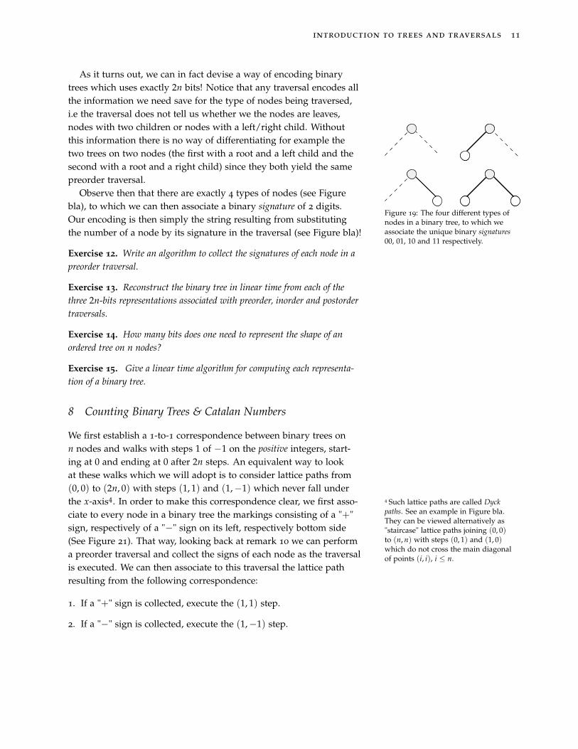
As it turns out, we can in fact devise a way of encoding binarytrees which uses exactly 2n bits! Notice that any traversal encodes allthe information we need save for the type of nodes being traversed,i.e the traversal does not tell us whether we the nodes are leaves,nodes with two children or nodes with a left/right child. Withoutthis information there is no way of differentiating for example thetwo trees on two nodes (the first with a root and a left child and thesecond with a root and a right child) since they both yield the samepreorder traversal.

Figure 19: The four different types ofnodes in a binary tree, to which weassociate the unique binary signatures00, 01, 10 and 11 respectively.

Observe then that there are exactly 4 types of nodes (see Figurebla), to which we can then associate a binary signature of 2 digits.Our encoding is then simply the string resulting from substitutingthe number of a node by its signature in the traversal (see Figure bla)!

Exercise 12. Write an algorithm to collect the signatures of each node in apreorder traversal.

Exercise 13. Reconstruct the binary tree in linear time from each of thethree 2n-bits representations associated with preorder, inorder and postordertraversals.

Exercise 14. How many bits does one need to represent the shape of anordered tree on n nodes?

Exercise 15. Give a linear time algorithm for computing each representa-tion of a binary tree.

8 Counting Binary Trees & Catalan Numbers

We first establish a 1-to-1 correspondence between binary trees onn nodes and walks with steps 1 of −1 on the positive integers, start-ing at 0 and ending at 0 after 2n steps. An equivalent way to lookat these walks which we will adopt is to consider lattice paths from(0, 0) to (2n, 0) with steps (1, 1) and (1,−1) which never fall underthe x-axis4. In order to make this correspondence clear, we first asso- 4 Such lattice paths are called Dyck

paths. See an example in Figure bla.They can be viewed alternatively as"staircase" lattice paths joining (0, 0)to (n, n) with steps (0, 1) and (1, 0)which do not cross the main diagonalof points (i, i), i ≤ n.

ciate to every node in a binary tree the markings consisting of a "+"sign, respectively of a "−" sign on its left, respectively bottom side(See Figure 21). That way, looking back at remark 10 we can performa preorder traversal and collect the signs of each node as the traversalis executed. We can then associate to this traversal the lattice pathresulting from the following correspondence:

1. If a "+" sign is collected, execute the (1, 1) step.

2. If a "−" sign is collected, execute the (1,−1) step.

introduction to trees and traversals 12

+

+ ++

+

+

− −

−

−

− −

(0,0) (2n,0)

Figure 20: Seeing binary trees as Dyckpaths.

+ +

+

+ + +

−

−

−

−

− −Figure 21: The markings describingthe bijection between binary trees andDyck paths. A preorder traversal of thistree would collect the markings in thefollowing order: ++−+−−++−−+−.

This clearly defines a lattice path from (0, 0) to (2n, 0) since at theend of the traversal, all the signs have been collected and "+" and "−"signs are present exactly in equal amount. It is not hard either to seethat the path stays positive (does not cross the x-axis) since for eachsingle node, the preorder traversal necessarily collects the "+" signfirst (we start going along the coastline down from the left side of theroot).

We have thus established that:

#(bin. trees on n nodes

)= #

(positive paths: (0, 0) → (2n, 0)

)Since all the lattice paths which fail to be positive necessarily cross

the line ` with y-coordinate −1 we can rewrite the number of posi-tive lattice paths as the following difference:

#(

paths: (0, 0) → (2n, 0))− #(

paths: (0, 0) → (2n, 0) meeting `)

The number of (all the) lattice paths from (0, 0) to (2n, 0) is sim-ply (2n

n ). Indeed for such a path, we need to go up exactly n timesand down exactly n times as well, there are then (2n

n ) different waysof choosing at what step we ought to go up or down (the steps atwhich we go up, resp. down steps constitute a subset of size n insidethe set of all 2n steps).

Now all that is left to do is count the number of lattice paths start-ing at (0, 0) and ending at (2n, 0) which cross the line `. Considersuch a lattice path and note that either the path crosses ` or it staysabove it.

Suppose then the path under consideration crosses ` and look atthe first point of crossing of this path with `. We can then performa reflection of the remaining section of the path across ` to obtain apath which will now end at (2n,−2). We can perform this operationfor any given path which crosses ` (see Figure 22). But notice aswell that any lattice path from (0, 0) to (2n,−2) must necessarily

introduction to trees and traversals 13

(0,0) (2n,0)

Figure 22: A lattice path crossing theline ` of ordinate −1 and the corre-sponding pivot point and reflected path(shown in grey).

cross `. So this reversible process of reflection defines a bijectionbetween paths from (0, 0) to (2n, 0) crossing ` and paths from (0, 0)to (2n,−2). Following our previous reasoning it is immediate thatthe number of paths joining (0, 0) to (2n,−2) is equal to ( 2n

n+1) =

( 2nn−1) (there are now n + 1 down steps, or n− 1 up steps).

We thus obtain that the number of lattice paths staying above thex-axis is precisely: (

2nn

)−(

2nn + 1

)=

1n + 1

(2nn

)This number is called the n-th Catalan number5.

5 The Catalan numbers appear in a lotof counting problems in combinatoricsand there is a plethora of well-knownbijections between sets of objects whichare counted by Catalan numbers. Fora reference see [2], [5], [4] or [3] for amore introductory presentation of someof these bijections. Among the mostfamous ones we mention the number ofbalanced bracketings/parenthesizationsof a given string of n + 1 charactersand the number of triangulations of aconvex (n + 2)-gon.

Figure 23: A pictorial description ofthe bijection between binary trees andtriangulations on convex (n + 2)-gons.

9 Arithmetic Expressions

9.1 Expression Trees

The problem of evaluating arithmetic expressions is an interestingexample of the use of binary trees and traversals. Notice indeed thatany arithmetic operation involves exactly two operands and we cantherefore construct an expression tree for any arithmetic expressionwhere the internal nodes correspond to the operators and the leavesthe operands (see Figure 24). Different traversals of such an expres-sion tree correspond to different notation systems:

A

B C

D E

+ ×

/

×

Figure 24: The expression tree corre-sponding to the arithmetic expression" A+(B×C)

D×E "

1. The Prefix/Polish notation corresponds to a preorder traversal of theexpression tree.

Example: / + A× B C× D E

2. The Postfix/Reverse Polish notation corresponds to a postordertraversal of the expression tree6. 6 Postfix notation is used for example in

the PostScript language.Example: A B C×+D E× /

introduction to trees and traversals 14

9.2 Evaluating Postfix Expressions

If given a postfix expression we can evaluate it using the followingsimple algorithm relying on a stack:

evaluate(E)

1 // The input is an arithmetic expression/string E in postfix2 // notation, consisting of a concatenation of characters x ∈ E3 // which are thus all either operands or (binary) operators

4 makenull(S)5 for x ∈ E (read from left to right)6 if x ∈ {Operands}7 push(x, S)8 else9 A←− pop(S)

10 B←− pop(S)11 C ←− AxB12 push(C, S)13 Return pop(S)

Exercise 16. How many bits suffice to store the shape of an n-node expres-sion tree ?

References

[1] Donald E Knuth. The Art of Computer Programming, Volumes1-4A Boxed Set. Addison-Wesley Professional, 2011. ISBN 978-0321751041.

[2] Igor Pak. Catalan numbers page. URL https://www.math.ucla.

edu/~pak/lectures/Cat/pakcat.htm.

[3] Richard P Stanley. Catalan numbers. URL http://www-math.

mit.edu/~rstan/transparencies/china.pdf?fbclid=

IwAR1LrjTdL7OZ3xeaPfJmxultM7a8EoiMXW4usSIxq2ugBO5Ck66Dg1pVGTA.

[4] Richard P. Stanley. Enumerative Combinatorics, volume II. Cam-bridge University Press, 2nd edition, 1999. ISBN 0-521-56069-1.

[5] Richard P. Stanley. Enumerative Combinatorics, volume I. Cam-bridge University Press, 2nd edition, 2012. ISBN 978-1-107-01545-5.