Time Series Analysis:Introduction to time series and forecasting

Handout 1: Introduction

Laura Mayoral

IAE and Barcelona GSE

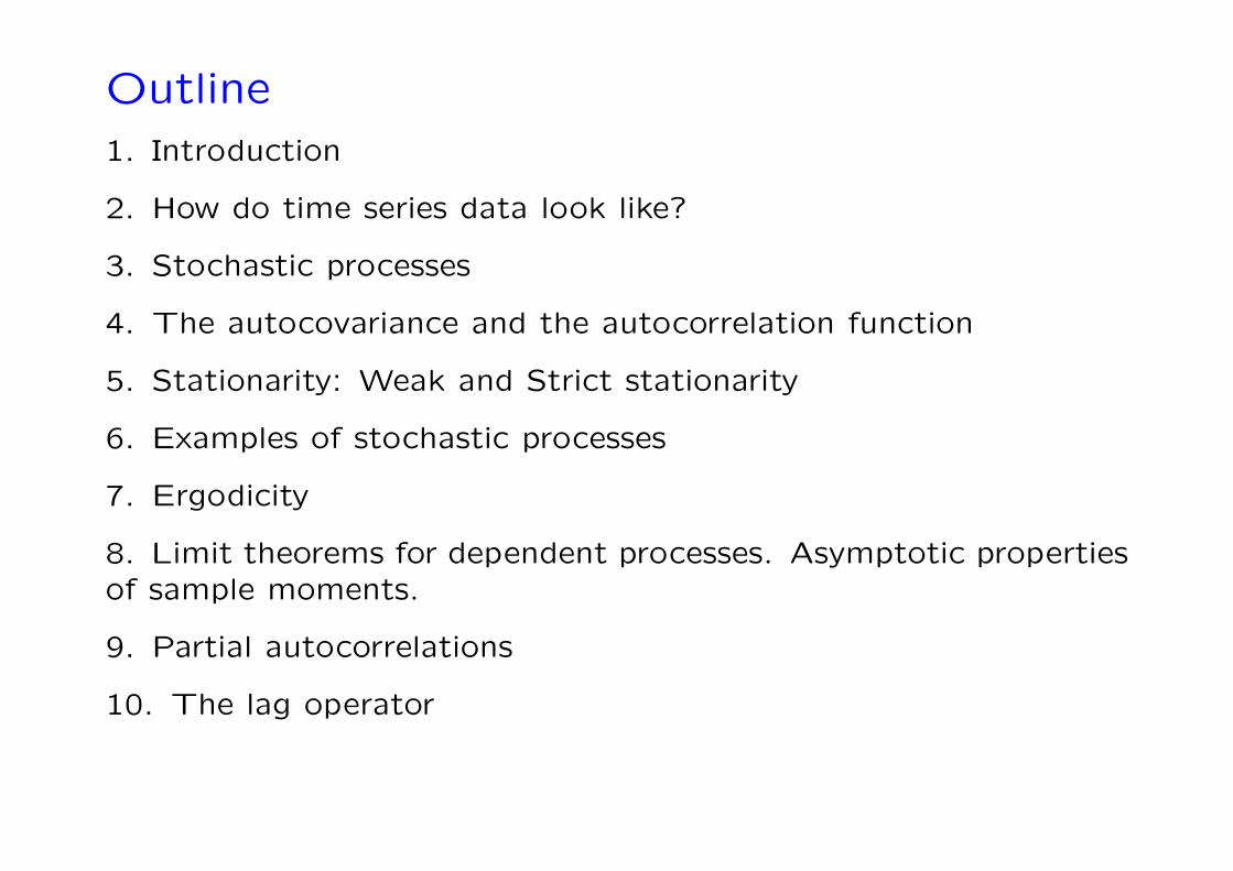
Outline1. Introduction

2. How do time series data look like?

3. Stochastic processes

4. The autocovariance and the autocorrelation function

5. Stationarity: Weak and Strict stationarity

6. Examples of stochastic processes

7. Ergodicity

8. Limit theorems for dependent processes. Asymptotic propertiesof sample moments.

9. Partial autocorrelations

10. The lag operator

0-1

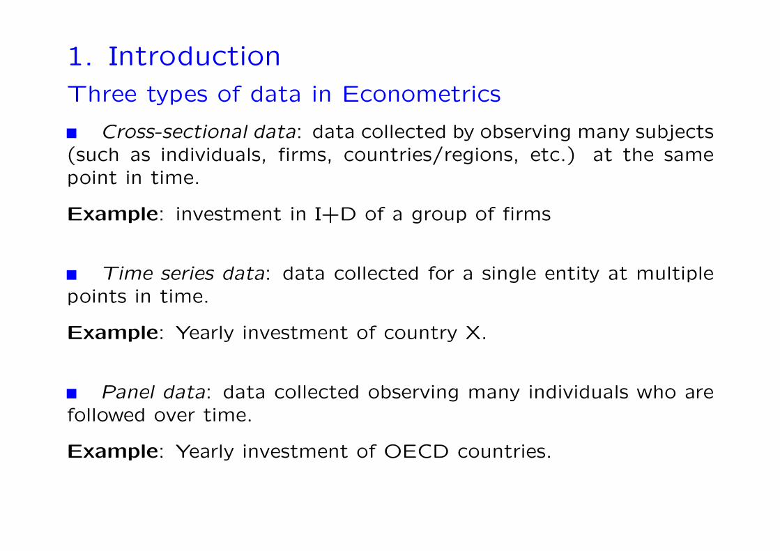
1. IntroductionThree types of data in Econometrics

Cross-sectional data: data collected by observing many subjects(such as individuals, firms, countries/regions, etc.) at the samepoint in time.

Example: investment in I+D of a group of firms

Time series data: data collected for a single entity at multiplepoints in time.

Example: Yearly investment of country X.

Panel data: data collected observing many individuals who arefollowed over time.

Example: Yearly investment of OECD countries.

0-2

Time series data can answer questions for which cross-sectionaldata might be inadequate.

What is the dynamic causal effect on a variable of interest, Y,of a change in another variable, X over time?

What is the best forecast of the value of some variable at afuture date?

Examples:

What is the effect of a change of monetary policy in output andinflation, both initially and subsequently?

What is the best forecast of inflation and output for the nextthree terms?

0-3

Time Series DataA time series is a set of observations

y1, y2, . . . , yt, . . . , yT ,

where t is the time index.

Time series data come with a natural temporal ordering

0-4

In cross-sectional analysis: observations (yi,xi), i = 1, ...,Nare randomly drawn from a fixed population. N observations fromthe same distribution. No ordering.

Random sampling implies that observations from different unitsare independently distributed.

In time series, we only have one observation from each variable(at each moment in time t). We don’t have random sampling.

Time series observations (yt,xt) , t = 1, ...T are in general non-independent.

−→ Dependence among observations is a key feature in time seriesvariables.

0-5

2. How do economic time series look like?

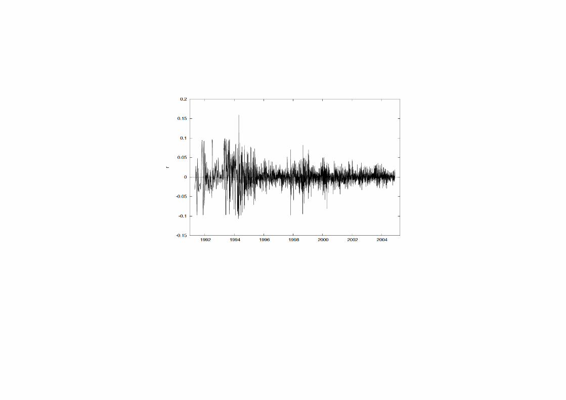
Time series are widely employed in empirical macroeconomics,finance, marketing, etc. Some examples are GNP, aggregate con-sumption, unemployment, population, exchange rates, inflation,stock returns...

Key features of economic time series are: trended behavior, sea-sonality and cyclical movements around trends.

In these links you can find many examples of economic time seriesdata:

https://fred.stlouisfed.org

http://www.economagic.com

http://www.nber.org/links/data.html

0-6

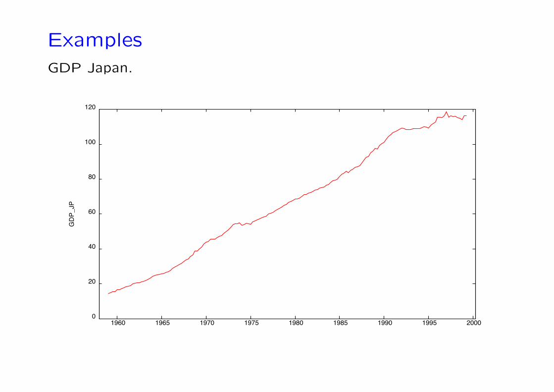
ExamplesGDP Japan.

0-7

0-8

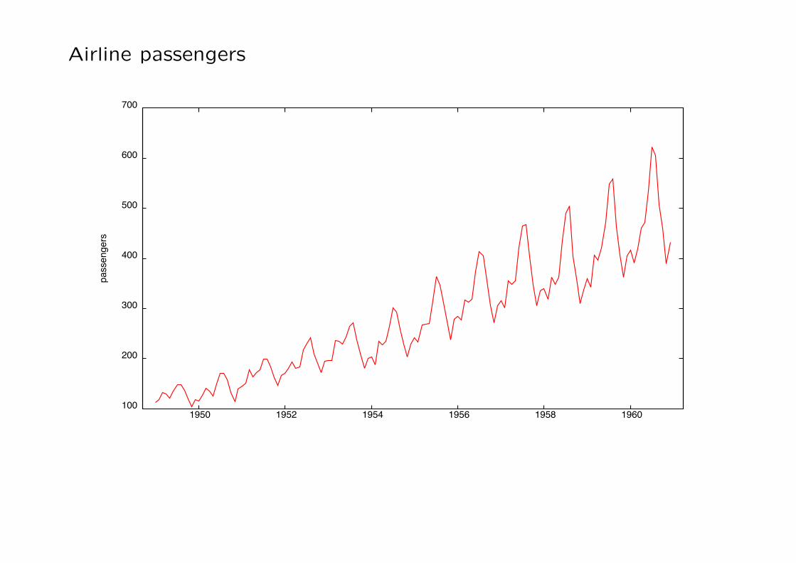
Airline passengers

0-9

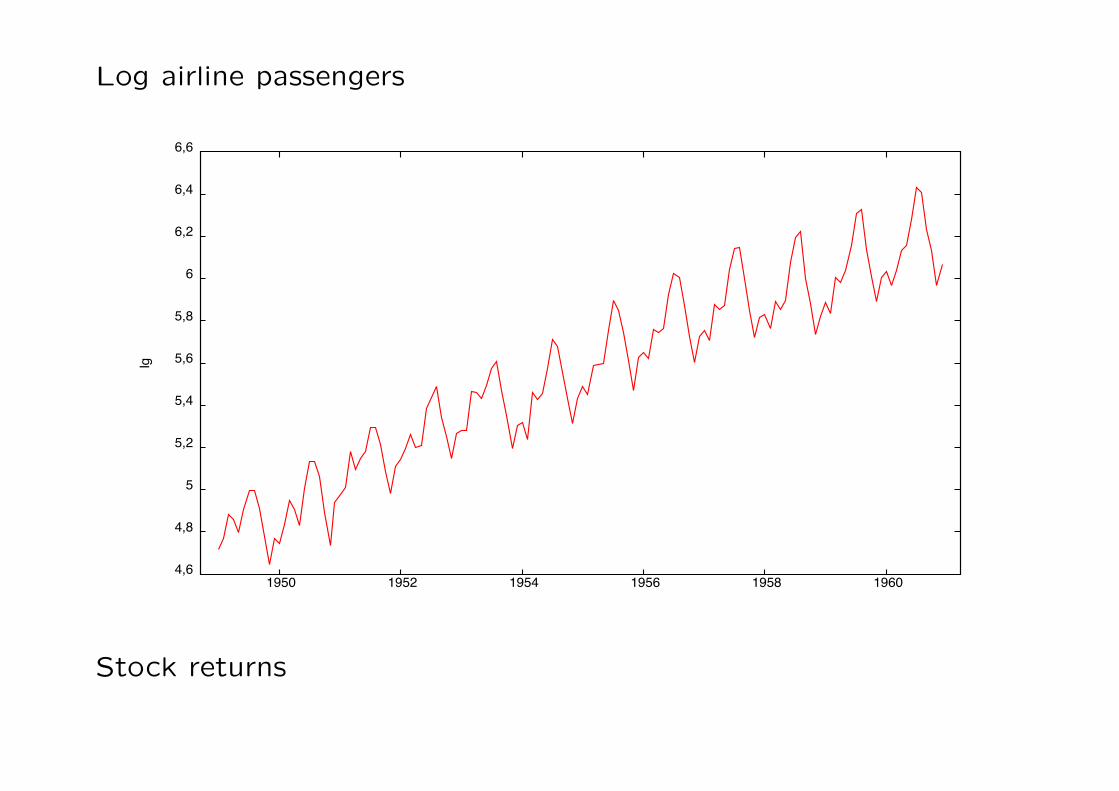
Log airline passengers

Stock returns

0-10

0-11

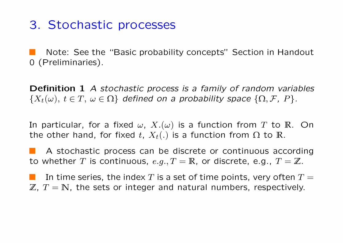
3. Stochastic processes

Note: See the “Basic probability concepts” Section in Handout0 (Preliminaries).

Definition 1 A stochastic process is a family of random variablesXt(ω), t ∈ T , ω ∈ Ω defined on a probability space Ω,F, P.

In particular, for a fixed ω, X.(ω) is a function from T to R. Onthe other hand, for fixed t, Xt(.) is a function from Ω to R.

A stochastic process can be discrete or continuous accordingto whether T is continuous, e.g.,T = R, or discrete, e.g., T = Z.

In time series, the index T is a set of time points, very often T =Z, T = N, the sets or integer and natural numbers, respectively.

0-12

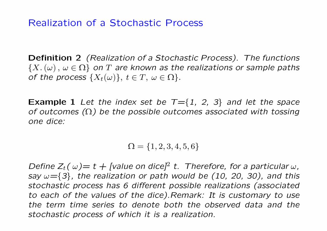
Realization of a Stochastic Process

Definition 2 (Realization of a Stochastic Process). The functionsX. (ω) , ω ∈ Ω on T are known as the realizations or sample pathsof the process Xt(ω), t ∈ T , ω ∈ Ω.

Example 1 Let the index set be T=1, 2, 3 and let the spaceof outcomes (Ω) be the possible outcomes associated with tossingone dice:

Ω = 1, 2, 3, 4, 5, 6

Define Zt( ω)= t + [value on dice]2 t. Therefore, for a particular ω,say ω=3, the realization or path would be (10, 20, 30), and thisstochastic process has 6 different possible realizations (associatedto each of the values of the dice).Remark: It is customary to usethe term time series to denote both the observed data and thestochastic process of which it is a realization.

0-13

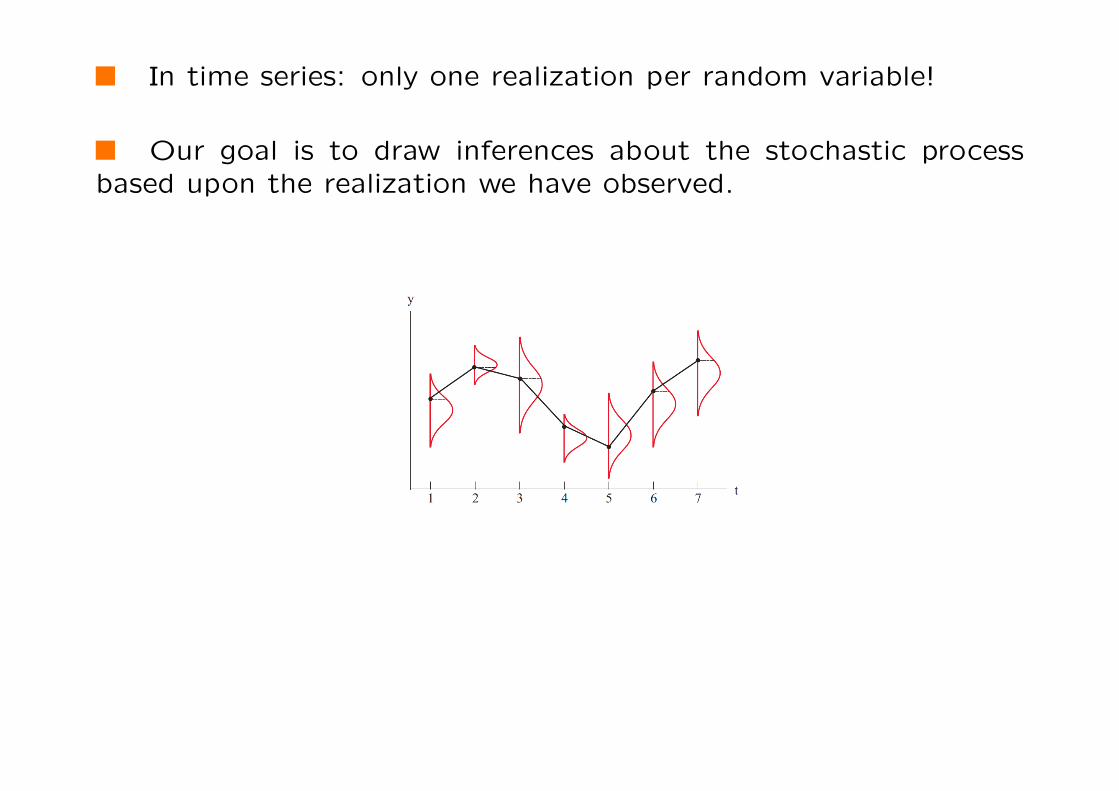
In time series: only one realization per random variable!

Our goal is to draw inferences about the stochastic processbased upon the realization we have observed.

0-14

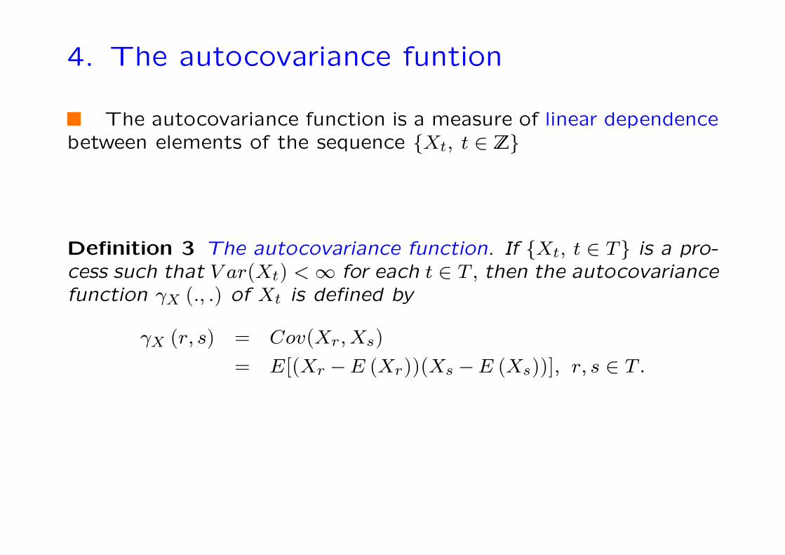
4. The autocovariance funtion

The autocovariance function is a measure of linear dependencebetween elements of the sequence Xt, t ∈ Z

Definition 3 The autocovariance function. If Xt, t ∈ T is a pro-cess such that V ar(Xt) <∞ for each t ∈ T , then the autocovariancefunction γX (., .) of Xt is defined by

γX (r, s) = Cov(Xr,Xs)

= E[(Xr −E (Xr))(Xs −E (Xs))], r, s ∈ T .

0-15

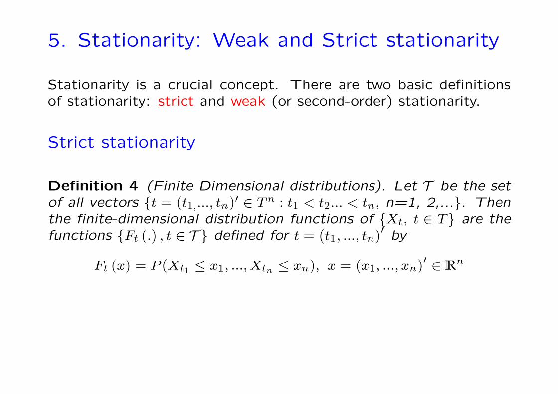
5. Stationarity: Weak and Strict stationarity

Stationarity is a crucial concept. There are two basic definitionsof stationarity: strict and weak (or second-order) stationarity.

Strict stationarity

Definition 4 (Finite Dimensional distributions). Let T be the setof all vectors t = (t1,..., tn)′ ∈ Tn : t1 < t2... < tn, n=1, 2,.... Thenthe finite-dimensional distribution functions of Xt, t ∈ T are thefunctions Ft (.) , t ∈ T defined for t = (t1, ..., tn)

′ by

Ft (x) = P (Xt1 ≤ x1, ...,Xtn ≤ xn), x = (x1, ...,xn)′ ∈ Rn

0-16

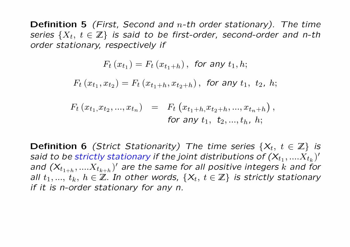
Definition 5 (First, Second and n-th order stationary). The timeseries Xt, t ∈ Z is said to be first-order, second-order and n-thorder stationary, respectively if

Ft (xt1) = Ft (xt1+h) , for any t1,h;

Ft (xt1 ,xt2) = Ft (xt1+h,xt2+h) , for any t1, t2, h;

Ft (xt1,xt2 , ...,xtn) = Ft(xt1+h,xt2+h, ...,xtn+h

),

for any t1, t2, ..., th, h;

Definition 6 (Strict Stationarity) The time series Xt, t ∈ Z issaid to be strictly stationary if the joint distributions of (Xt1 , ....Xtk )

′

and (Xt1+h , ....Xtk+h)′ are the same for all positive integers k and for

all t1, ..., tk, h ∈ Z. In other words, Xt, t ∈ Z is strictly stationaryif it is n-order stationary for any n.

0-17

Interpretation:

This means that the graphs over two equal-length time intervalsof a realization of the time series should exhibit similar statisticalcharacteristics.

Joint distribution functions are difficult to work with. Thefollowing concept introduces a notion of stationarity that can becharacterised just by looking at first and second moments.

0-18

Weak Stationarity

Definition 7 (Weak Stationarity) The time series Xt, t ∈ Z issaid to be weakly stationary if

i) E∣∣X2

t

∣∣ <∞ for all t ∈ Z

ii) E(Xt) = m for all t

iii) γX (r, s) = γX (r + t, s+ t) for all r, s, t ∈ Z.

This concept of stationarity is usually referred in the literatureas weak stationarity or covariance stationarity.

0-19

Notice that stationarity requires also the variance of Xt to beconstant. If Xt is stationary, then

V ar(Xr) = γX(r, r) = γX (r + t, r + t) = V ar(Xr+t),

for all r, t ∈ Z.

Stationarity basically means that the mean, the variance arefinite and constant and that the autocovariance function only de-pends on h, the distance between observations.

0-20

Stationarity and the autocovariance funtion

If Xt, t ∈ Z is stationary, then γX (r, s) = γX(r− s, 0) for all r,s ∈ Z. Then, for stationary processes one can define the autoco-variance as a function of only one parameter, that is

γX(h) = Cov(Xt+h,Xt) for all t,h ∈ Z.

The function γX (.) will be referred to as the autocovariancefunction of the process Xt and γX(h) is the value of this functionat lag h.

Notation: γX(h) or simply γh will denote the h-th autocovari-ance of Xt.

0-21

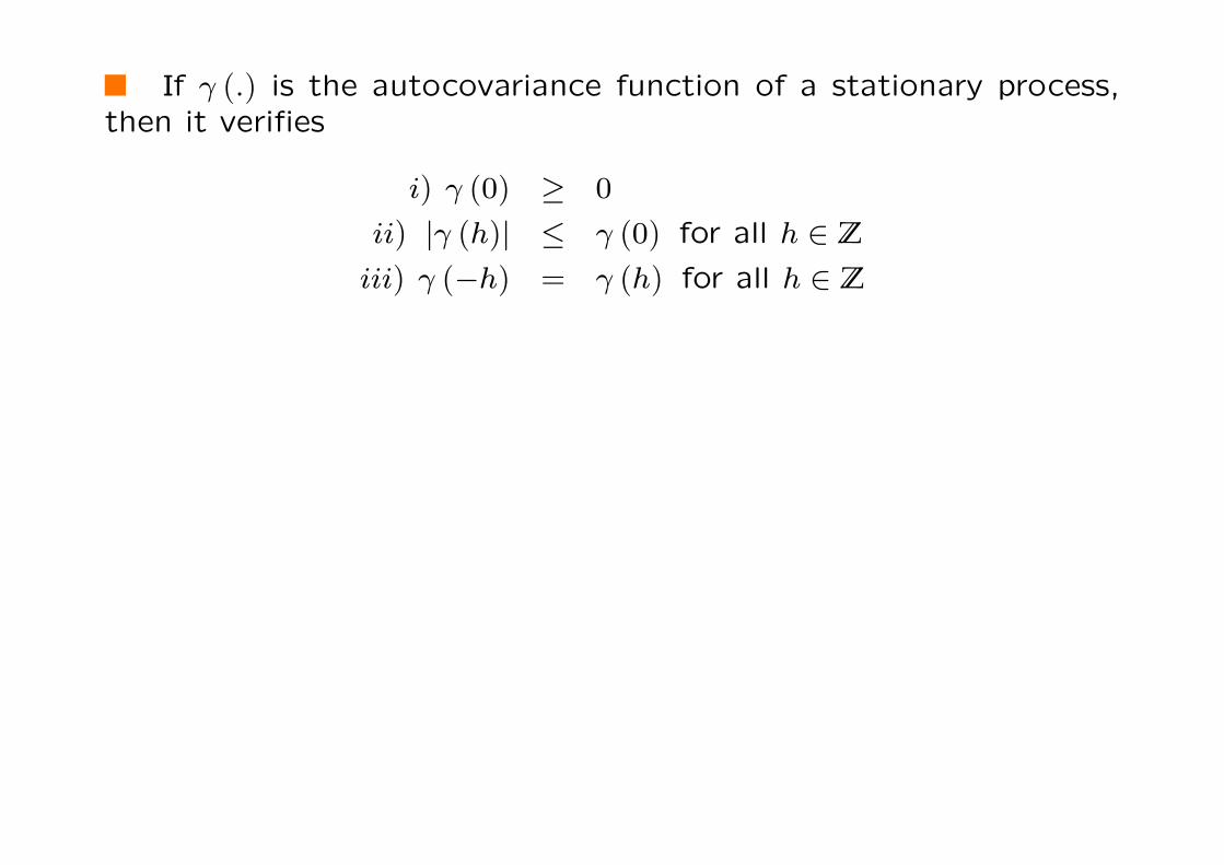
If γ (.) is the autocovariance function of a stationary process,then it verifies

i) γ (0) ≥ 0

ii) |γ (h)| ≤ γ (0) for all h ∈ Z

iii) γ (−h) = γ (h) for all h ∈ Z

0-22

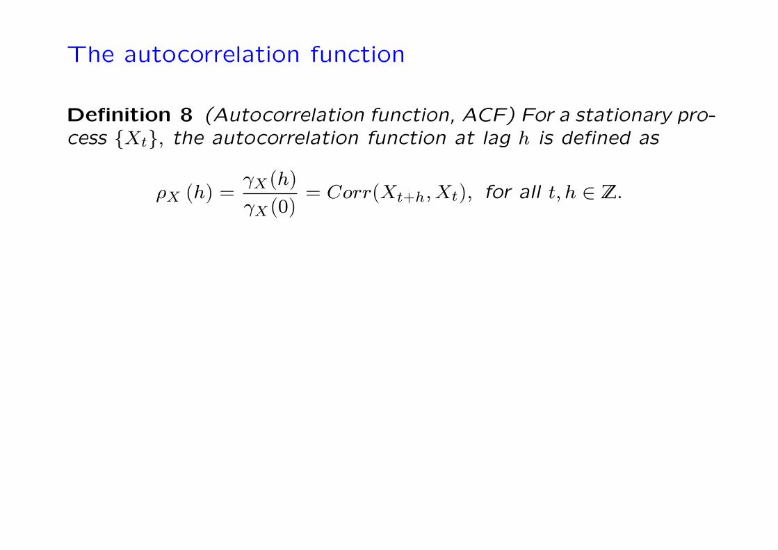
The autocorrelation function

Definition 8 (Autocorrelation function, ACF) For a stationary pro-cess Xt, the autocorrelation function at lag h is defined as

ρX (h) =γX(h)

γX(0)= Corr(Xt+h,Xt), for all t,h ∈ Z.

0-23

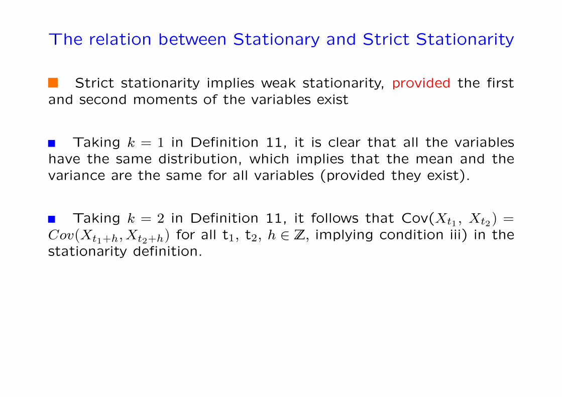
The relation between Stationary and Strict Stationarity

Strict stationarity implies weak stationarity, provided the firstand second moments of the variables exist

Taking k = 1 in Definition 11, it is clear that all the variableshave the same distribution, which implies that the mean and thevariance are the same for all variables (provided they exist).

Taking k = 2 in Definition 11, it follows that Cov(Xt1 , Xt2) =Cov(Xt1+h,Xt2+h) for all t1, t2, h ∈ Z, implying condition iii) in thestationarity definition.

0-24

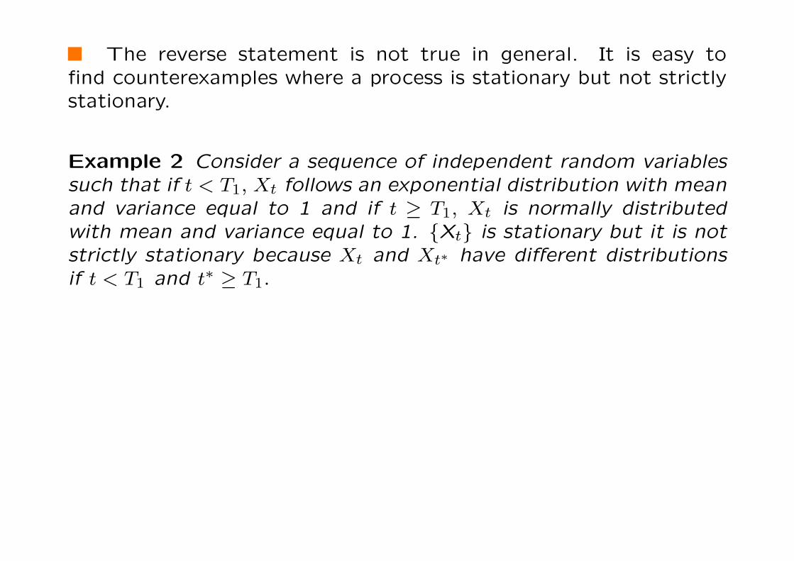
The reverse statement is not true in general. It is easy tofind counterexamples where a process is stationary but not strictlystationary.

Example 2 Consider a sequence of independent random variablessuch that if t < T1, Xt follows an exponential distribution with meanand variance equal to 1 and if t ≥ T1, Xt is normally distributedwith mean and variance equal to 1. Xt is stationary but it is notstrictly stationary because Xt and Xt∗ have different distributionsif t < T1 and t∗ ≥ T1.

0-25

The relation between Stationary and Strict Stationarity,II

There is an one important case where both concepts of stationaryare equivalent.

Definition 9 (Gaussian Time series) The process Xt is a Gaus-sian time series if and only if the distribution functions of Xt areall multivariate normal.

If Xt, t ∈ Z is a stationary Gaussian time series, then it is alsostrictly stationary, since for all n ∈ 1, 2, ... and for all h, t1 , t2, ...∈ Z, the random vectors (Xt1 , ...,Xtn)

′, and (Xt1+h, ...,Xtn+h)

′ havethe same mean, and covariance matrix, and hence they have thesame distribution.

0-26

6. Some examples of stationary processes

Example 3 iid sequences.

The sequence εt is i.i.d (independent and identically dis-tributed) if all the variables are independent and share the sameunivariate distribution.

Clearly, an iid sequence is strictly stationary and provided thefirst and second order moments exist, it is also weak stationary.

Example 4 White noise process.

The process εt is called white noise if it is weakly stationarywith E (εt) = 0 and autovariance function

γε (h) =

σ2 h = 00 h 6= 0

0-27

The white noise process is important because is used as abuilding block for more general processes, as can be seen in someof the examples below.

An i.i.d sequence with zero mean and variance σ2 is also whitenoise. The converse is not true in general. Furthermore, a whitenoise process might not be strictly stationary.

0-28

Example 5 Martingale difference sequence, m.d.s.

A process εt, with E (εt) = 0 is called a martingale differencesequence if

E (εt|εt−1, εt−2, ...) = 0, for t ≥ 2.

It can be shown that if E (εt) = 0 and the second order momentsexist then,

εt is i.i.d.⇒ εt is m.d.s⇒ εt is white noise

but the converse implication is not true in general.

0-29

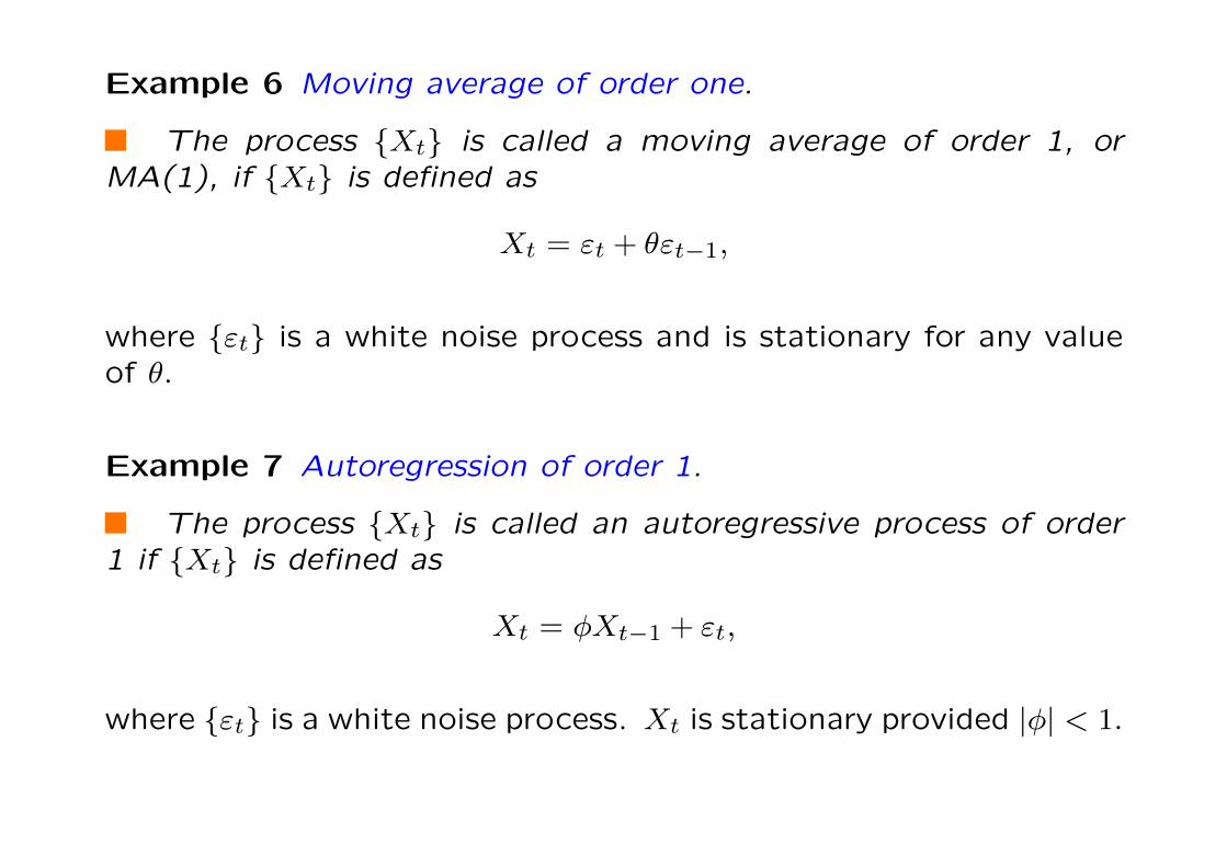
Example 6 Moving average of order one.

The process Xt is called a moving average of order 1, orMA(1), if Xt is defined as

Xt = εt + θεt−1,

where εt is a white noise process and is stationary for any valueof θ.

Example 7 Autoregression of order 1.

The process Xt is called an autoregressive process of order1 if Xt is defined as

Xt = φXt−1 + εt,

where εt is a white noise process. Xt is stationary provided |φ| < 1.

0-30

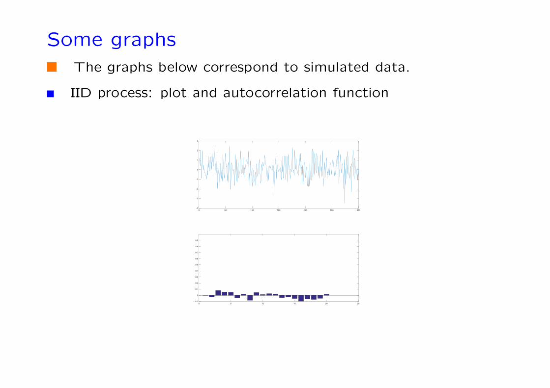
Some graphsThe graphs below correspond to simulated data.

IID process: plot and autocorrelation function

0 50 100 150 200 250 300

-4

-3

-2

-1

0

1

2

3

0 5 10 15 20 25

-0.1

0

0.1

0.2

0.3

0.4

0.5

0.6

0.7

0.8

0.9

0-31

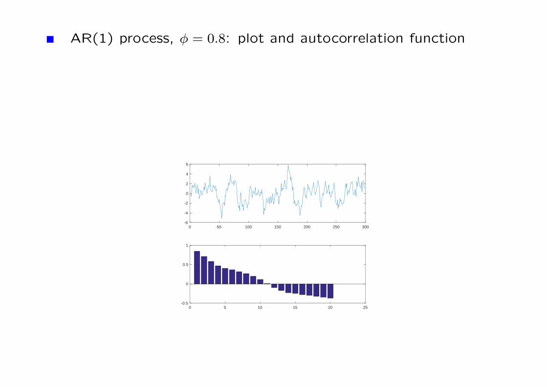
AR(1) process, φ = 0.8: plot and autocorrelation function

0 50 100 150 200 250 300-6

-4

-2

0

2

4

6

0 5 10 15 20 25-0.5

0

0.5

1

0-32

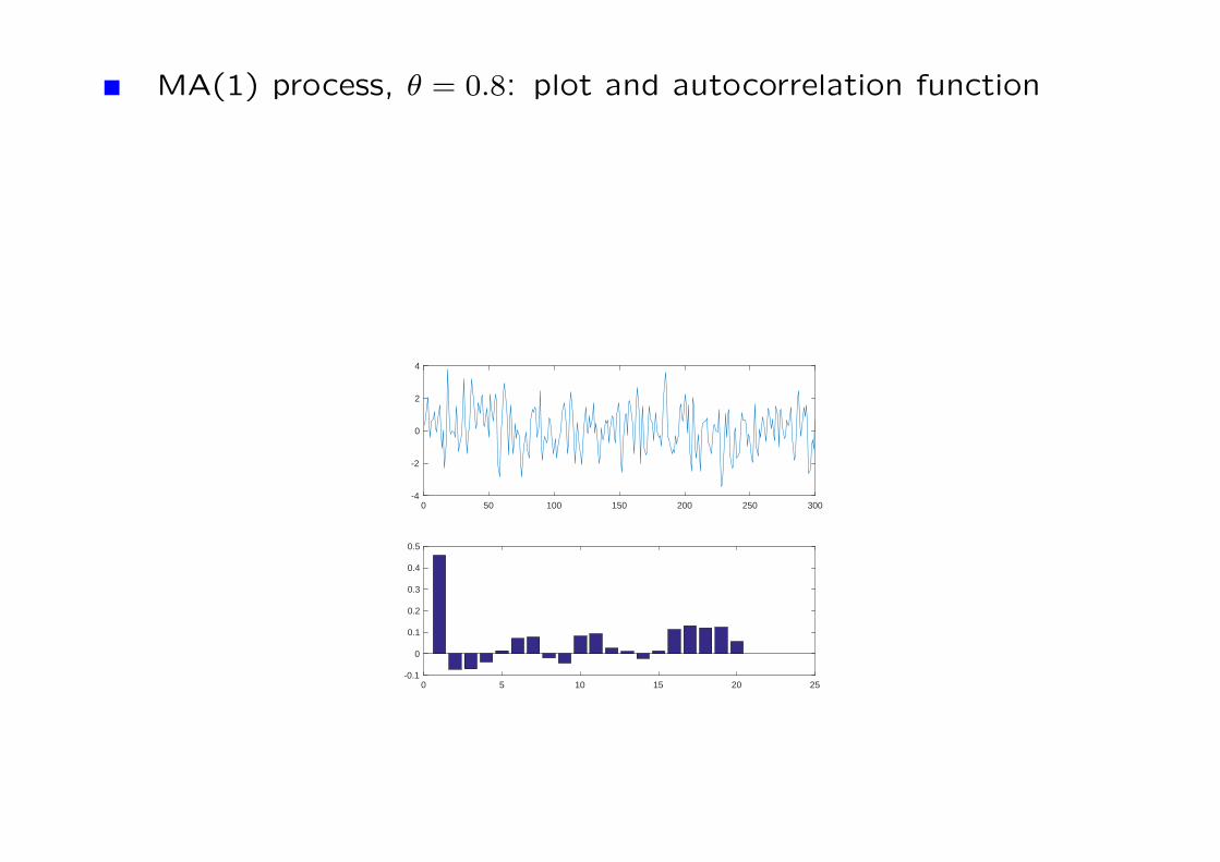
MA(1) process, θ = 0.8: plot and autocorrelation function

0 50 100 150 200 250 300-4

-2

0

2

4

0 5 10 15 20 25-0.1

0

0.1

0.2

0.3

0.4

0.5

0-33

Some examples of non-stationary processes

Example 8 A trended process.

Xt = βt+ εt,

where t = 1, ....,T is a deterministic time trend.

Example 9 A random walk process

Xt = Xt−1 + εt, t≥0

Example 10 A process with a break

Xt = εt, t < k

Xt = µ+ εt, t ≥ k

where µ 6= 0.

0-34

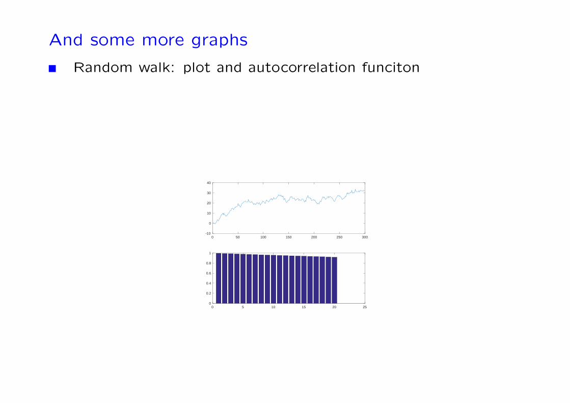
And some more graphs

Random walk: plot and autocorrelation funciton

0 50 100 150 200 250 300-10

0

10

20

30

40

0 5 10 15 20 250

0.2

0.4

0.6

0.8

1

0-35

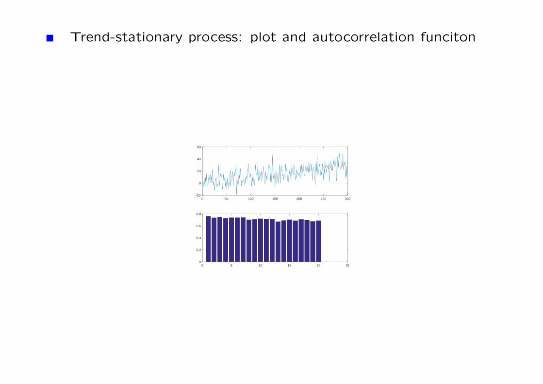
Trend-stationary process: plot and autocorrelation funciton

0 50 100 150 200 250 300-20

0

20

40

60

0 5 10 15 20 250

0.2

0.4

0.6

0.8

0-36

7. Ergodicity

Note: Please review the section “Asymptotic theory” in Hand-out 0 to refresh the definition of convergence of random variables,limit theorems, etc.

Ergodicity is a condition that restricts the memory of the pro-cess.

A loose definition of ergodicity is that the process is asymptoti-cally independent. That is, for sufficiently large n, Xi and Xi+n arenearly independent. A more formal definition is provided below. Allof these definitions essentially say that the effect of current eventseventually disappears.

0-37

Ensemble averages versus time averages

Consider a stationary stochastic proces Xt, with E (Xt) = µfor all t. Consider the estimation of µ.

The standard approach for estimating the mean of a singlerandom variable consists of computing its sample mean

X = N−1N∑i=1

X(i)t , i = 1, ...N , (1)

where X(i)t are different realizations of the variable Xt. We will

referred to expression (1) as the ’ensemble average’.

When working in a laboratory (or when dealing with cross sec-tional data), one could generate different observations for the vari-able Xt under identical conditions.

0-38

When analyzing economic variables over time, we can only ob-serve a unique realization for each of the random variables Xt.Thus, it is not possible to estimate µ by computing the ensembleaverage (1).

However, we can compute a time average

X = T−1T∑t=1

Xt (2)

Whether time averages such as (2) converge to the same limitas the ensemble average, E(Xt), has to do with the concept ofErgodicity.

0-39

Ergodicity for the mean and Ergodicity for second mo-ments

Definition 10 (Ergodicity for the mean) A covariance stationaryprocess Xt is said to be ergodic for the mean if (2) converges toE(Xt) .

Definition 11 (Ergodicity for the second moments) A covariancestationary process is said to be ergodic for the second moments if

1

(T − j)

∑t=j+1

(Yt − µ) (Yt−j − µ)p→ γj , for all j.

0-40

Ergodicity and Stationarity are two different concepts

In many applications, ergodicity and stationarity turn out toamount to the same requirements. However, they are two differentconcepts

Stationarity is a necessary (but not sufficient) condition forergodicity

0-41

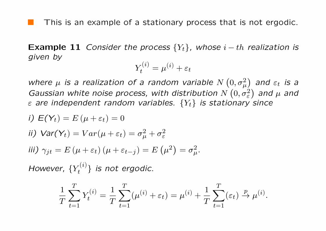
This is an example of a stationary process that is not ergodic.

Example 11 Consider the process Yt, whose i− th realization isgiven by

Y(i)t = µ(i) + εt

where µ is a realization of a random variable N(0,σ2µ

)and εt is a

Gaussian white noise process, with distribution N(0,σ2ε

)and µ and

ε are independent random variables. Yt is stationary since

i) E(Yt) = E (µ+ εt) = 0

ii) Var(Yt) = V ar(µ+ εt) = σ2µ + σ2ε

iii) γjt = E (µ+ εt) (µ+ εt−j) = E(µ2)= σ2µ.

However, Y (i)t is not ergodic.

1

T

T∑t=1

Y(i)t =

1

T

T∑t=1

(µ(i) + εt) = µ(i) +1

T

T∑t=1

(εt)p→ µ(i).

0-42

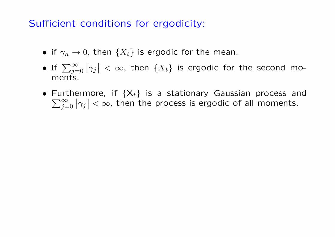
Sufficient conditions for ergodicity:

• if γn → 0, then Xt is ergodic for the mean.

• If∑∞

j=0

∣∣γj∣∣ < ∞, then Xt is ergodic for the second mo-ments.

• Furthermore, if Xt is a stationary Gaussian process and∑∞j=0

∣∣γj∣∣ <∞, then the process is ergodic of all moments.

0-43

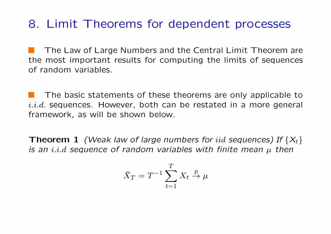
8. Limit Theorems for dependent processes

The Law of Large Numbers and the Central Limit Theorem arethe most important results for computing the limits of sequencesof random variables.

The basic statements of these theorems are only applicable toi.i.d. sequences. However, both can be restated in a more generalframework, as will be shown below.

Theorem 1 (Weak law of large numbers for iid sequences) If Xtis an i.i.d sequence of random variables with finite mean µ then

XT = T−1T∑t=1

Xtp→ µ

0-44

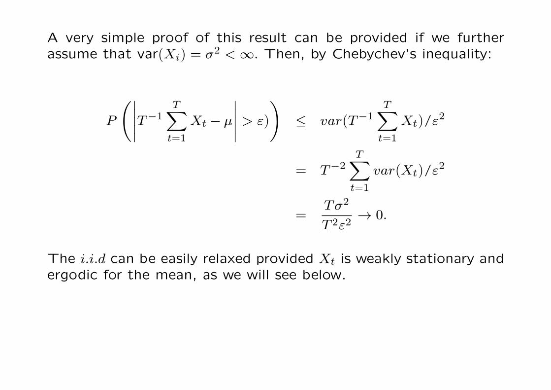
A very simple proof of this result can be provided if we furtherassume that var(Xi) = σ2 <∞. Then, by Chebychev’s inequality:

P

(∣∣∣∣∣T−1T∑t=1

Xt − µ

∣∣∣∣∣ > ε)

)≤ var(T−1

T∑t=1

Xt)/ε2

= T−2T∑t=1

var(Xt)/ε2

=Tσ2

T 2ε2→ 0.

The i.i.d can be easily relaxed provided Xt is weakly stationary andergodic for the mean, as we will see below.

0-45

Theorem 2 (Central limit theorem for i.i.d. sequences) If Xt isa sequence of iid(µ, σ2) random variables then

√T (XT − µ)/σ

d→ N(0, 1).

A more general version of this theorem can be stated as follows.

Theorem 3 (Central limit theorem for martingale difference se-quences) Let Xt be a martingale difference sequence. If a)

E(X2t

)= σ2t > 0 with T−1

∑Tt=1 σ

2t → σ2, b) E(|Xt|)r <∞ for some

r ¿2 and all t and c) T−1∑X2t

p→ σ2, then√TXT

d→ N(0,σ2

).

0-46

Application: Asymptotic properties of the sample mo-ments of a stationary process

Consider the estimation of the first and second moments ofa stationary process Xt (i.e, mean, variance and autocovariancefuncton).

We next show

1) how to estimate these quantities and

2) the asymptotic properties of these estimators

0-47

The sample mean of a stationary process

The sample mean is the natural estimator for the expected valueof a process.

Definition 12 Let Xt be a process. The sample mean is definedas

XT = T−1T∑t=1

Xt.

Theorem 4 If Xt is stationary with mean µ and autocovariancefunction γ (.) , then

i) E(XT ) = µ

ii) If γ (T )→ 0 as T→∞, Var(XT ) = E(XT − µ)2 → 0.

iii) If∑∞

h=−∞ |γ (h)| <∞, TE(XT − µ)2 →∑∞

h=−∞ γ(h).

Proof. See Brockell and Davis, (1991), p. 219.

0-48

Notice that i) and ii) imply that XT converges in mean squareto µ.

thus, the sample mean is consistent provided γ (T ) → 0 (re-member that this is the ergodicity condition).

Then, this theorem presents a weak Law of Large Numbersfor stationary and ergodic processes.

Stationarity alone is not enough. Consider this example: V∼N(0,σ2

). Suppose Xt = V for all t. Then, Xt is stationary and

cov(Xt,Xs) = σ2 for all t, s. Notice that covariances are notsummable and that a LLN does not hold. Why? This exampleis equivalent of having a single observation of a random variable.

0-49

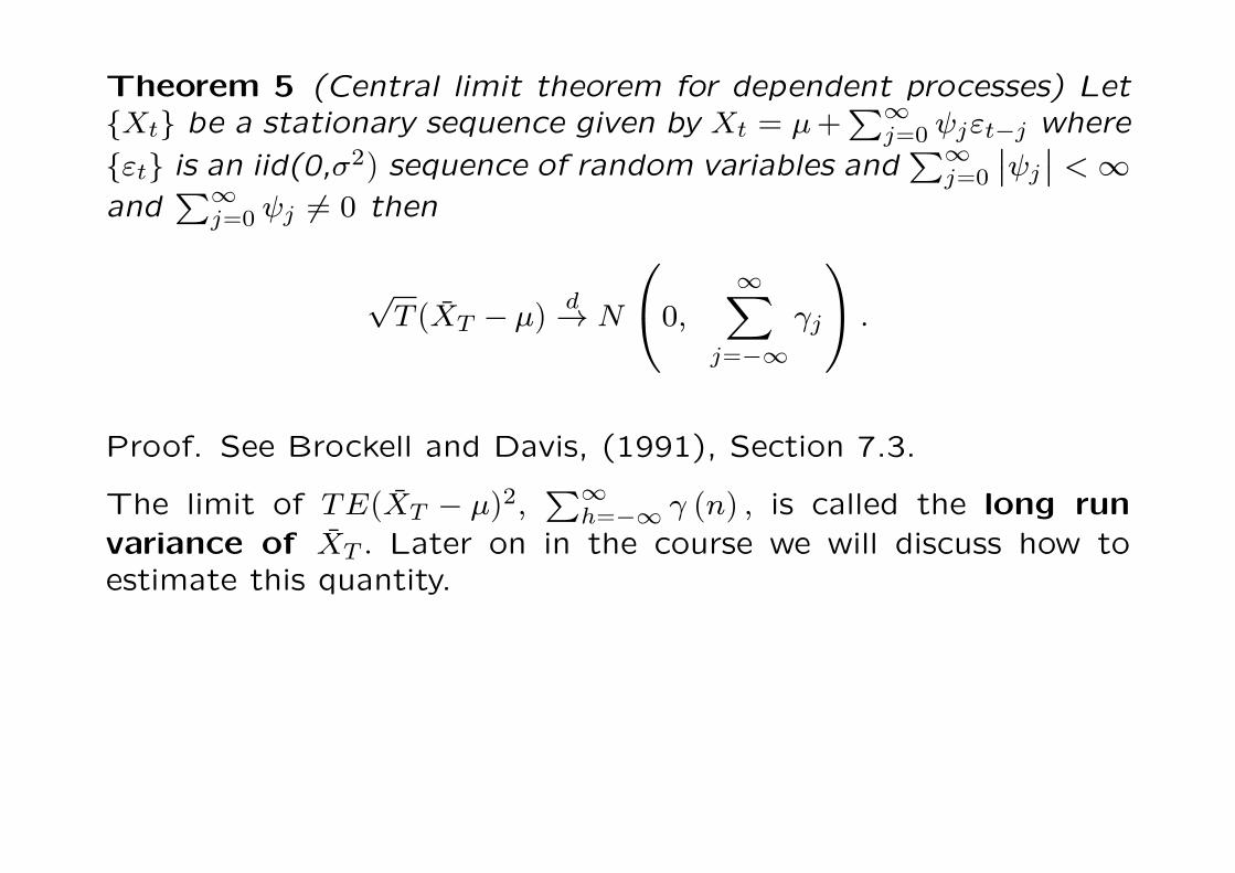
Theorem 5 (Central limit theorem for dependent processes) LetXt be a stationary sequence given by Xt = µ+

∑∞j=0 ψjεt−j where

εt is an iid(0,σ2) sequence of random variables and∑∞

j=0

∣∣ψj∣∣ <∞and

∑∞j=0 ψj 6= 0 then

√T (XT − µ)

d→ N

0,∞∑

j=−∞γj

.

Proof. See Brockell and Davis, (1991), Section 7.3.

The limit of TE(XT − µ)2,∑∞

h=−∞ γ (n) , is called the long runvariance of XT . Later on in the course we will discuss how toestimate this quantity.

0-50

Sample autocovariance and sample autocorrelation

Definition 13 The sample autocovariance of x1, x2, ..., xT isdefined as

γ (h) = T−1T−h∑j=1

(xj+h − XT

)(xj − XT ) , 0 ≤ h ≤ T , (3)

where XT = T−1∑T

j=1 xj .

Definition 14 The sample autocorrelation of x1, x2, ..., xT isdefined as

ρ (h) =γ (h)

γ (0), 0 ≤ h ≤ T . (4)

The estimators in (3) and in (4) are biased but under certainconditions they are asymptotically unbiased.

0-51

A remark:

The sample autocovariance and sample autocorrelation can becomputed for any data set, and are not restricted to realizationsof a stationary process.

For stationary processes both functions will show a rapid decaytowards zero as h increases.

However, for non-stationary data, these functions will exhibitquite different behavior. For data containing a trend, γ (h) andρ (h) will exhibit very slow decay as h increases and for data with asubstantial cyclical component, γ (h) and ρ (h) will exhibit a similarcyclical behavior with the same periodicity. Thus, γ (.), ρ (.) areoften employed as identification tools.

0-52

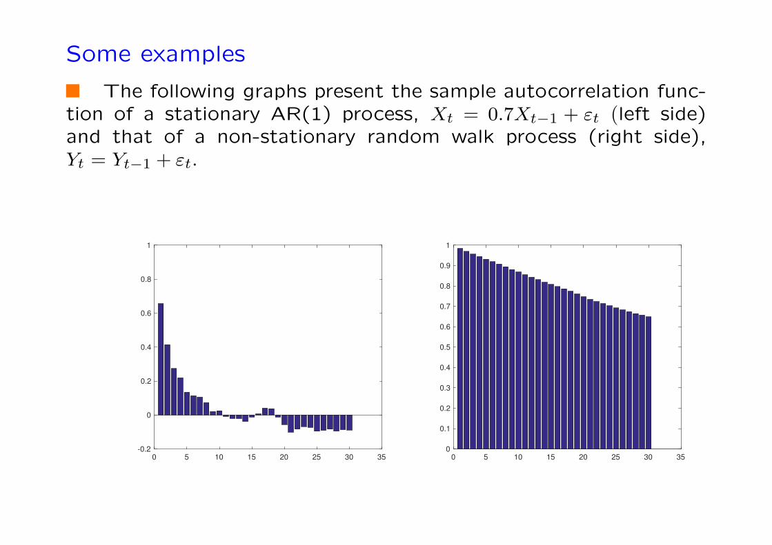
Some examples

The following graphs present the sample autocorrelation func-tion of a stationary AR(1) process, Xt = 0.7Xt−1 + εt (left side)and that of a non-stationary random walk process (right side),Yt = Yt−1 + εt.

0 5 10 15 20 25 30 35

-0.2

0

0.2

0.4

0.6

0.8

1

0 5 10 15 20 25 30 35

0

0.1

0.2

0.3

0.4

0.5

0.6

0.7

0.8

0.9

1

0-53

Asymptotic properties of the sample autocorrelation func-tion

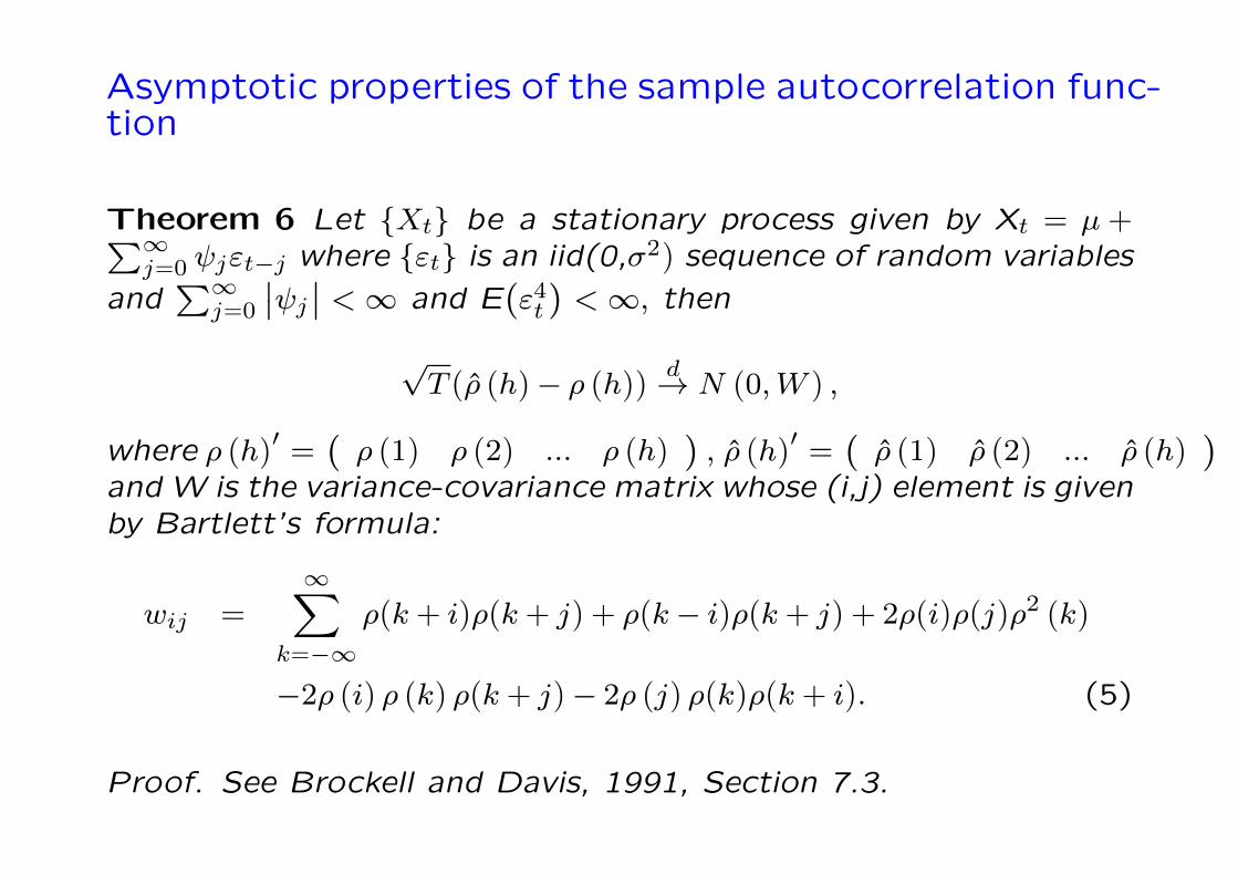
Theorem 6 Let Xt be a stationary process given by Xt = µ +∑∞j=0 ψjεt−j where εt is an iid(0,σ2) sequence of random variables

and∑∞

j=0

∣∣ψj∣∣ <∞ and E(ε4t)<∞, then

√T (ρ (h)− ρ (h)) d→ N (0,W ) ,

where ρ (h)′ =(ρ (1) ρ (2) ... ρ (h)

), ρ (h)′ =

(ρ (1) ρ (2) ... ρ (h)

)and W is the variance-covariance matrix whose (i,j) element is givenby Bartlett’s formula:

wij =∞∑

k=−∞ρ(k + i)ρ(k + j) + ρ(k− i)ρ(k + j) + 2ρ(i)ρ(j)ρ2 (k)

−2ρ (i) ρ (k) ρ(k + j)− 2ρ (j) ρ(k)ρ(k + i). (5)

Proof. See Brockell and Davis, 1991, Section 7.3.

0-54

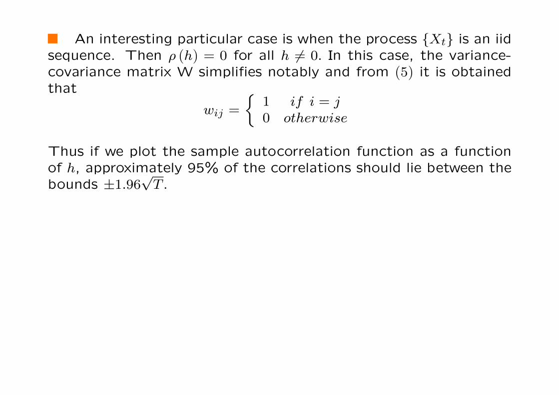
An interesting particular case is when the process Xt is an iidsequence. Then ρ (h) = 0 for all h 6= 0. In this case, the variance-covariance matrix W simplifies notably and from (5) it is obtainedthat

wij =

1 if i = j0 otherwise

Thus if we plot the sample autocorrelation function as a functionof h, approximately 95% of the correlations should lie between thebounds ±1.96

√T .

0-55

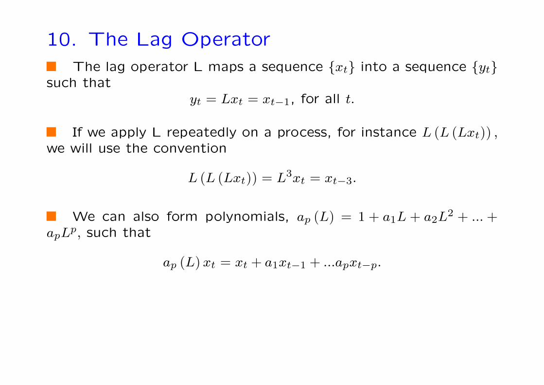
10. The Lag OperatorThe lag operator L maps a sequence xt into a sequence yt

such thatyt = Lxt = xt−1, for all t.

If we apply L repeatedly on a process, for instance L (L (Lxt)) ,we will use the convention

L (L (Lxt)) = L3xt = xt−3.

We can also form polynomials, ap (L) = 1 + a1L + a2L2 + ... +apLp, such that

ap (L) xt = xt + a1xt−1 + ...apxt−p.

0-56

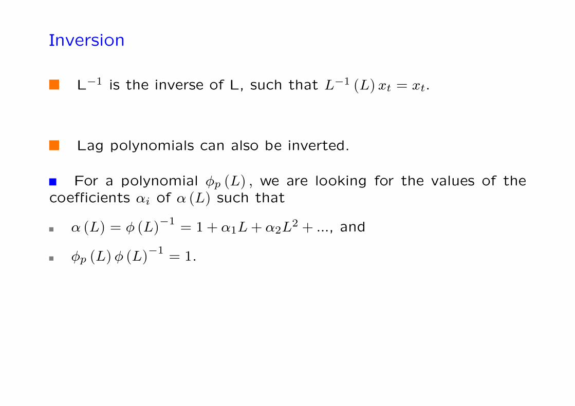
Inversion

L−1 is the inverse of L, such that L−1 (L) xt = xt.

Lag polynomials can also be inverted.

For a polynomial φp (L) , we are looking for the values of thecoefficients αi of α (L) such that

α (L) = φ (L)−1 = 1+ α1L+ α2L2 + ..., and

φp (L)φ (L)−1 = 1.

0-57

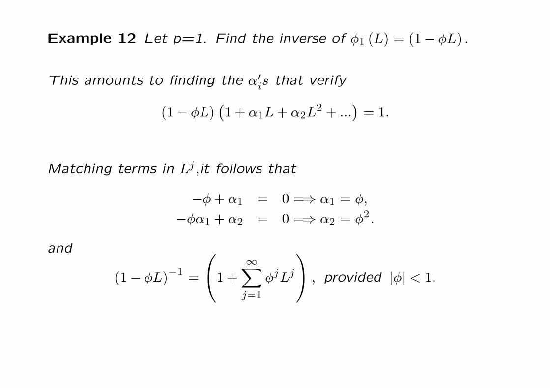
Example 12 Let p=1. Find the inverse of φ1 (L) = (1− φL) .

This amounts to finding the α′is that verify

(1− φL)(1+ α1L+ α2L

2 + ...)= 1.

Matching terms in Lj ,it follows that

−φ+ α1 = 0 =⇒ α1 = φ,

−φα1 + α2 = 0 =⇒ α2 = φ2.

and

(1− φL)−1 =

1+∞∑j=1

φjLj

, provided |φ| < 1.

0-58

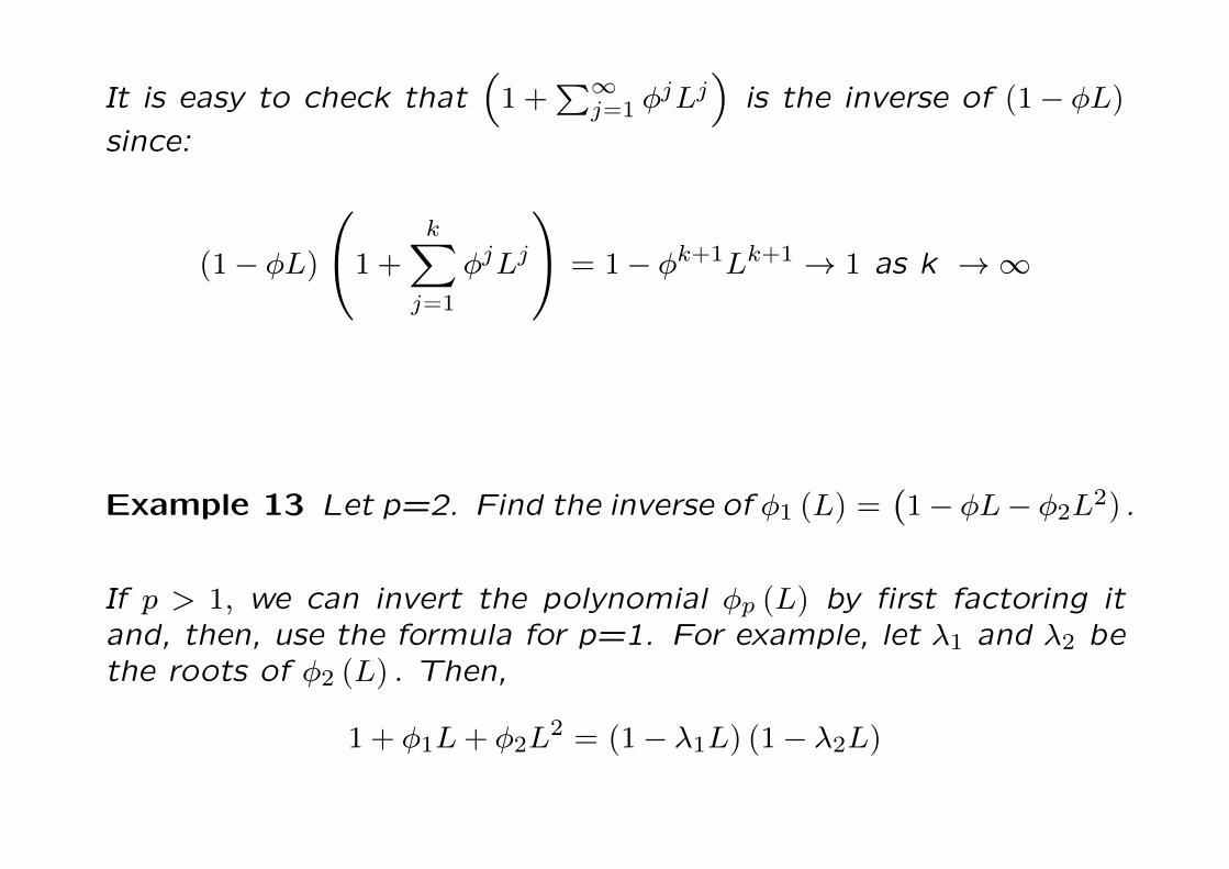
It is easy to check that(1+∑∞

j=1 φjLj)

is the inverse of (1− φL)since:

(1− φL)

1+k∑j=1

φjLj

= 1− φk+1Lk+1 → 1 as k →∞

Example 13 Let p=2. Find the inverse of φ1 (L) =(1− φL− φ2L2) .

If p > 1, we can invert the polynomial φp (L) by first factoring itand, then, use the formula for p=1. For example, let λ1 and λ2 bethe roots of φ2 (L) . Then,

1+ φ1L+ φ2L2 = (1− λ1L) (1− λ2L)

0-59

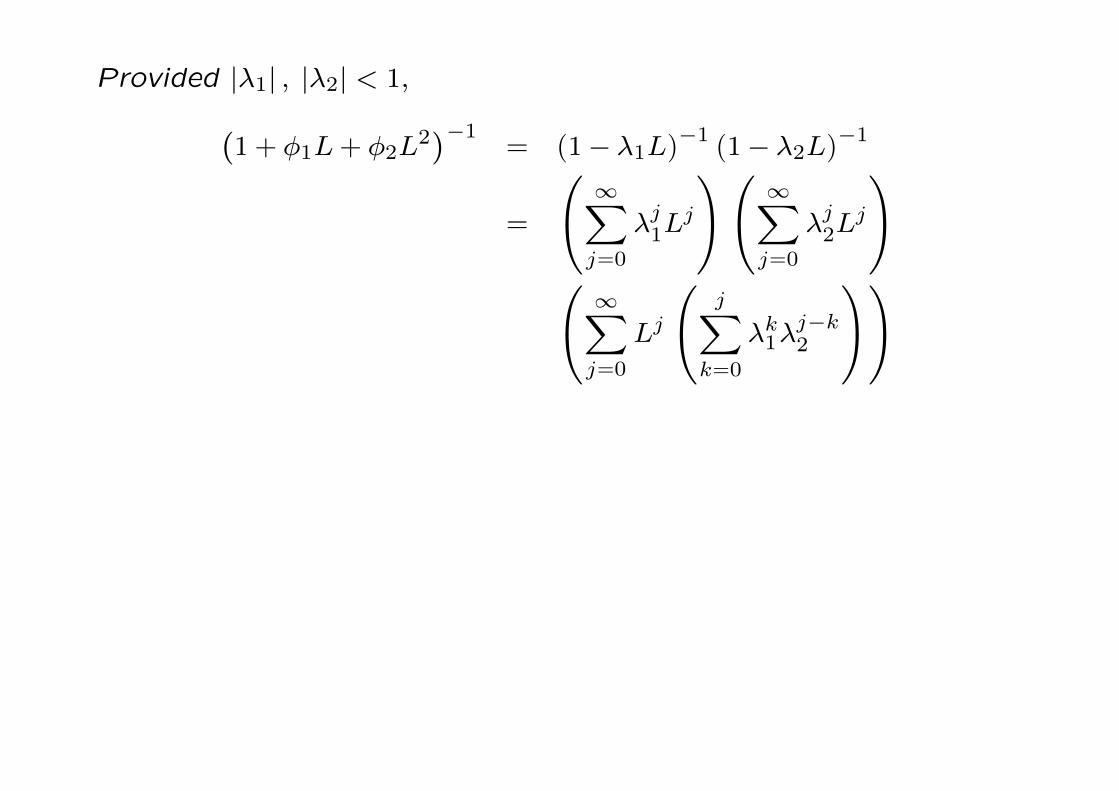
Provided |λ1| , |λ2| < 1,(1+ φ1L+ φ2L

2)−1

= (1− λ1L)−1 (1− λ2L)−1

=

∞∑j=0

λj1Lj

∞∑j=0

λj2Lj

∞∑j=0

Lj

j∑k=0

λk1λj−k2

0-60

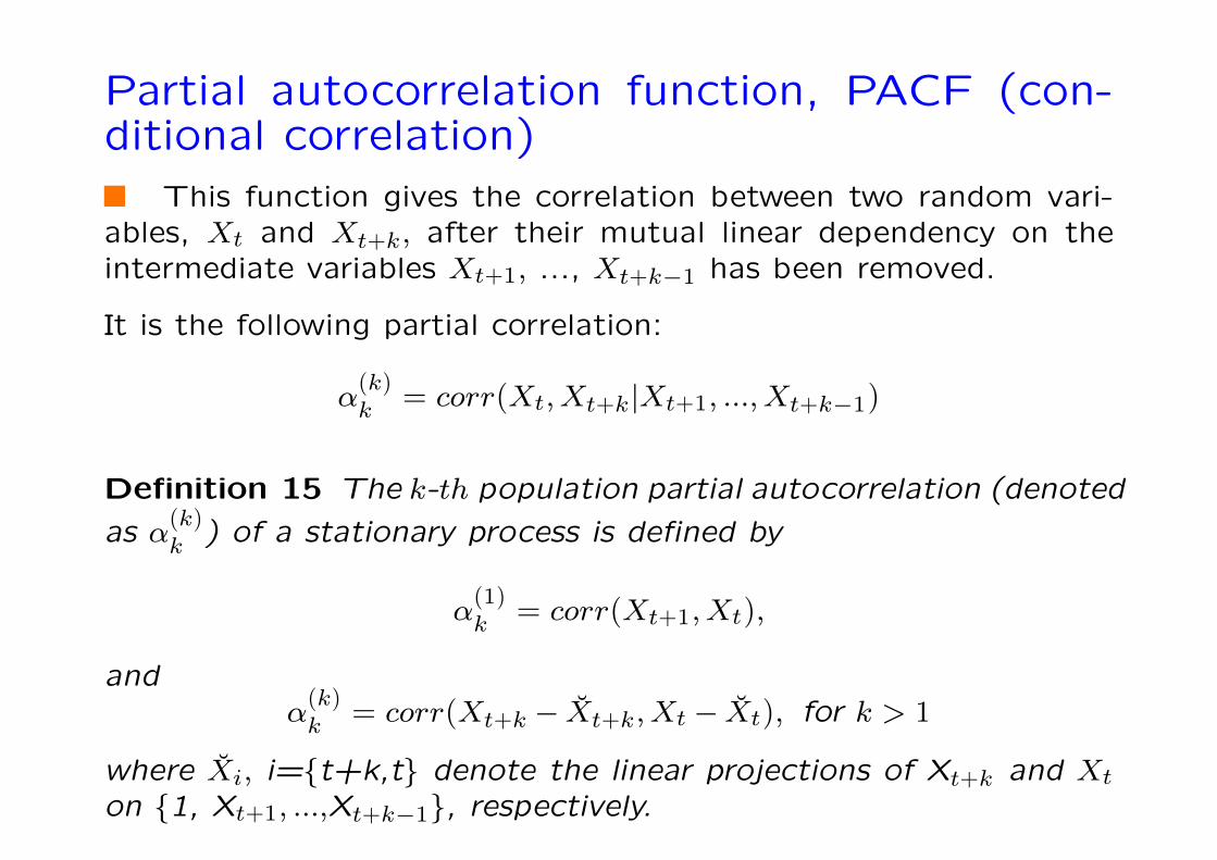
Partial autocorrelation function, PACF (con-ditional correlation)

This function gives the correlation between two random vari-ables, Xt and Xt+k, after their mutual linear dependency on theintermediate variables Xt+1, ..., Xt+k−1 has been removed.

It is the following partial correlation:

α(k)k = corr(Xt,Xt+k|Xt+1, ...,Xt+k−1)

Definition 15 The k-th population partial autocorrelation (denoted

as α(k)k ) of a stationary process is defined by

α(1)k = corr(Xt+1,Xt),

andα(k)k = corr(Xt+k − Xt+k,Xt − Xt), for k > 1

where Xi, i=t+k,t denote the linear projections of Xt+k and Xton 1, Xt+1, ...,Xt+k−1, respectively.

0-61

PACF: computation

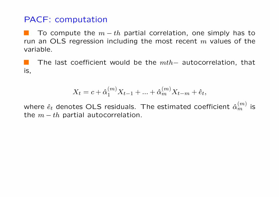
To compute the m− th partial correlation, one simply has torun an OLS regression including the most recent m values of thevariable.

The last coefficient would be the mth− autocorrelation, thatis,

Xt = c+ α(m)1 Xt−1 + ...+ α

(m)m Xt−m + et,

where et denotes OLS residuals. The estimated coefficient α(m)m is

the m− th partial autocorrelation.

0-62

ReferencesHamilton: Chapter 1, 7.

Brockwell, P. J., and A. Davis (1991): Chapter 1, 6.

Stock and Watson, Chapter 14.

0-63