Introduction to the very basic Introduction to the very basic computational aspects of the computational aspects of the

modern Quantum Chemistry for modern Quantum Chemistry for Software EngineersSoftware Engineers

Introduction to the very basic Introduction to the very basic computational aspects of the computational aspects of the

modern Quantum Chemistry for modern Quantum Chemistry for Software EngineersSoftware Engineers

Alexander A. GranovskyAlexander A. GranovskyThe PC GAMESS/Firefly Project

July 23, 2009MSU, Moscow, Russia

22

OutlineOutlineOutlineOutline

Quantum Chemistry: purpose and methods Quantum Chemistry: purpose and methods Typical tasks, their parameters and computational Typical tasks, their parameters and computational

complexitycomplexity Conventional, direct, and semi-direct methodsConventional, direct, and semi-direct methods Standard and “fast” methodsStandard and “fast” methods Typical parallel algorithms: key features and open Typical parallel algorithms: key features and open

problemsproblems– Canonical example – four index integral transformation Canonical example – four index integral transformation

stepstep

33

Quantum Chemistry: purpose and Quantum Chemistry: purpose and methodsmethods

Quantum Chemistry: purpose and Quantum Chemistry: purpose and methodsmethods

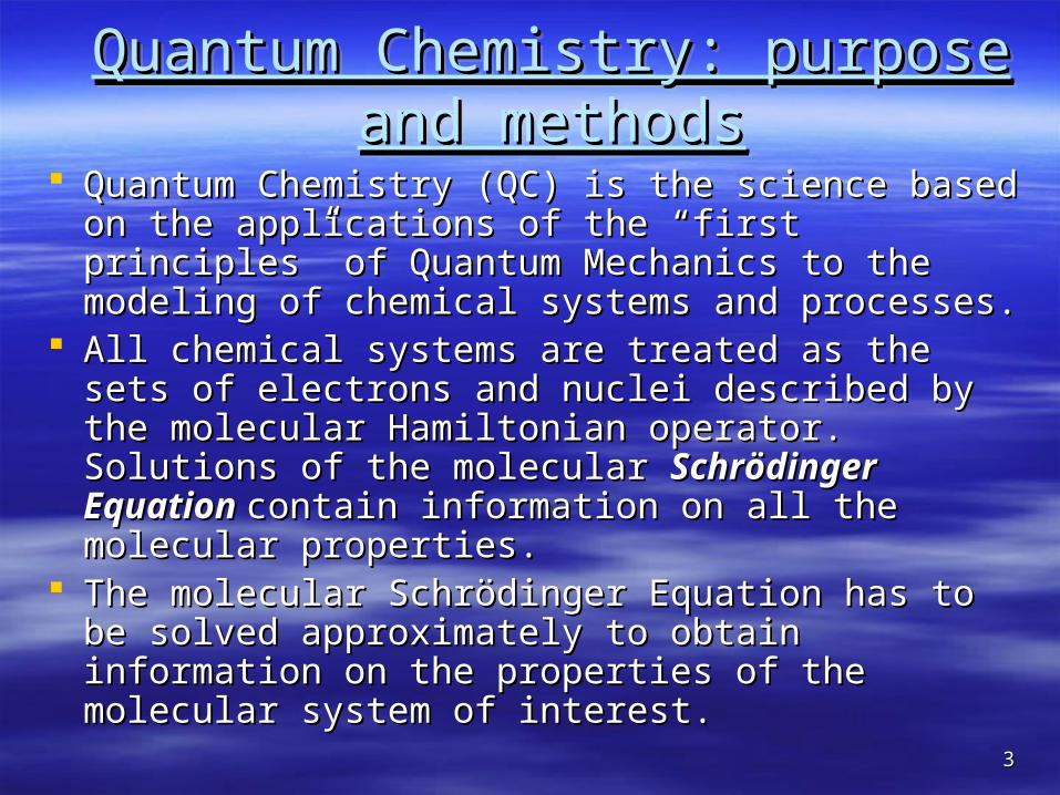
Quantum Chemistry (QC) is the science based on Quantum Chemistry (QC) is the science based on the applications of the “first principles” of Quantum the applications of the “first principles” of Quantum Mechanics to the modeling of chemical systems Mechanics to the modeling of chemical systems and processes.and processes.

All chemical systems are treated as the sets of All chemical systems are treated as the sets of electrons and nuclei described by the molecular electrons and nuclei described by the molecular Hamiltonian operator. Solutions of the molecular Hamiltonian operator. Solutions of the molecular SchrSchröödinger Equation dinger Equation contain information on all contain information on all the molecular properties.the molecular properties.

The molecular SchrThe molecular Schröödinger Equation has to be dinger Equation has to be solved approximately to obtain information on the solved approximately to obtain information on the properties of the molecular system of interest. properties of the molecular system of interest.

44

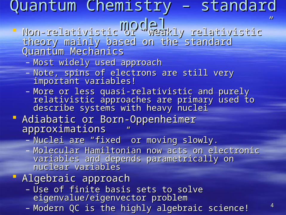
Quantum Chemistry – standard modelQuantum Chemistry – standard model Non-relativistic or “weakly relativistic” theory Non-relativistic or “weakly relativistic” theory

mainly based on the standard Quantum mainly based on the standard Quantum MechanicsMechanics– Most widely used approachMost widely used approach– Note, spins of electrons are still very important Note, spins of electrons are still very important

variables!variables!– More or less quasi-relativistic and purely relativistic More or less quasi-relativistic and purely relativistic

approaches are primary used to describe systems with approaches are primary used to describe systems with heavy nucleiheavy nuclei

Adiabatic or Born-Oppenheimer approximationsAdiabatic or Born-Oppenheimer approximations– Nuclei are “fixed” or moving slowly.Nuclei are “fixed” or moving slowly.– Molecular Hamiltonian now acts on electronic variables Molecular Hamiltonian now acts on electronic variables

and depends parametrically on nuclear variablesand depends parametrically on nuclear variables Algebraic approachAlgebraic approach

– Use of finite basis sets to solve eigenvalue/eigenvector Use of finite basis sets to solve eigenvalue/eigenvector problemproblem

– Modern QC is the highly algebraic science!Modern QC is the highly algebraic science!

55

Quantum Chemistry – algebraic Quantum Chemistry – algebraic approachapproach

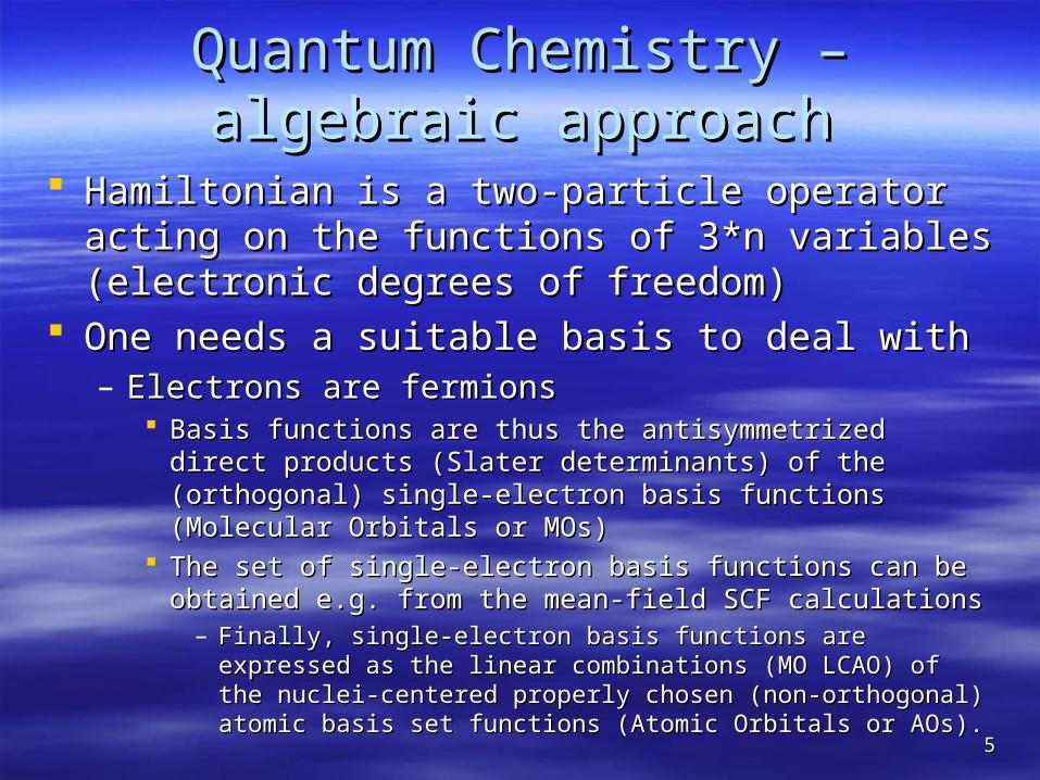
Hamiltonian is a two-particle operator acting on Hamiltonian is a two-particle operator acting on the functions of 3*n variables (electronic degrees the functions of 3*n variables (electronic degrees of freedom)of freedom)

One needs a suitable basis to deal withOne needs a suitable basis to deal with– Electrons are fermionsElectrons are fermions

Basis functions are thus the antisymmetrized direct products Basis functions are thus the antisymmetrized direct products (Slater determinants) of the (orthogonal) single-electron basis (Slater determinants) of the (orthogonal) single-electron basis functions (Molecular Orbitals or MOs)functions (Molecular Orbitals or MOs)

The set of single-electron basis functions can be obtained e.g. The set of single-electron basis functions can be obtained e.g. from the mean-field SCF calculationsfrom the mean-field SCF calculations

– Finally, single-electron basis functions are expressed as the linear Finally, single-electron basis functions are expressed as the linear combinations (MO LCAO) of the nuclei-centered properly chosen combinations (MO LCAO) of the nuclei-centered properly chosen (non-orthogonal) atomic basis set functions (Atomic Orbitals or (non-orthogonal) atomic basis set functions (Atomic Orbitals or AOs).AOs).

66

Some important factsSome important facts One needs the rules to compute matrix elements of One needs the rules to compute matrix elements of

Hamiltonian and other operatorsHamiltonian and other operators These are so-called Slater rulesThese are so-called Slater rules

– Most important consequences of the two-body nature of Most important consequences of the two-body nature of electronic Hamiltonianelectronic Hamiltonian Matrix elements can be expressed as the combinations of four-Matrix elements can be expressed as the combinations of four-

index quantities (ij|kl) - so called “two-electron integrals”index quantities (ij|kl) - so called “two-electron integrals”– Called “atomic integrals” in the original AO basis setCalled “atomic integrals” in the original AO basis set

((||))

– Called “molecular integrals” being transformed to the MO basisCalled “molecular integrals” being transformed to the MO basis (ij|kl)(ij|kl)

Simple consequence: use of four-index quantities Simple consequence: use of four-index quantities (tensors) are more or less unavoidable in QC!(tensors) are more or less unavoidable in QC!

77

Some important collisionsSome important collisions Let N be the number of atomic basis functions Let N be the number of atomic basis functions

(AOs) – the main parameter controlling complexity(AOs) – the main parameter controlling complexity– The native size of dense matrices typical to QC The native size of dense matrices typical to QC

methods is about of N by N, e.g. 1000x1000methods is about of N by N, e.g. 1000x1000 Relatively small matricesRelatively small matrices Has nothing common with HPLHas nothing common with HPL

– The native size of sparse matrices typical to QC The native size of sparse matrices typical to QC methods varies but is usually very large (e.g. up to ca. methods varies but is usually very large (e.g. up to ca. N!)N!) No any regular structure usually…No any regular structure usually…

– The native size of intermediate quantities to be The native size of intermediate quantities to be computed and reused can be up to Ncomputed and reused can be up to N44 (two-electron (two-electron integrals in MO basis) and more.integrals in MO basis) and more. 1000100044 double precision numbers would require 8 TBytes of double precision numbers would require 8 TBytes of

RAM or storageRAM or storage

88

Typical tasks, their parameters and Typical tasks, their parameters and computational complexitycomputational complexity

QC – myriads of QC – myriads of theoreticaltheoretical approximations approximations– To name just a few To name just a few

Hartree-Fock (Self-Consistent Field) and Density Functional TheoryHartree-Fock (Self-Consistent Field) and Density Functional Theory– Simplest Mean Field TheoriesSimplest Mean Field Theories

Perturbative approachesPerturbative approaches– Single-reference RS-type perturbation theoriesSingle-reference RS-type perturbation theories

MP2, MP3, MP4 etc…MP2, MP3, MP4 etc…– Various Multi-Reference and/or Quasi-Degenerate perturbation theoriesVarious Multi-Reference and/or Quasi-Degenerate perturbation theories

Configuration Interaction (CI)Configuration Interaction (CI)– Linear variational principleLinear variational principle

Lots of different types of CILots of different types of CI Coupled ClustersCoupled Clusters

– Truncated exponential AnsatzTruncated exponential Ansatz Lots of different approximations/variantsLots of different approximations/variants

Lots of multi-reference methods…Lots of multi-reference methods… Green functions, propagators and similar approaches…Green functions, propagators and similar approaches… Time-dependent approaches…Time-dependent approaches…

99

Quantum Chemistry – computation Quantum Chemistry – computation complexitycomplexity

Hartree-Fock (Self-Consistent Field) and Density Hartree-Fock (Self-Consistent Field) and Density Functional TheoryFunctional Theory– From NFrom N22 to N to N44

Perturbative approachesPerturbative approaches– NN55 at the second order, N at the second order, N66 at the third, N at the third, N77 at the fourth at the fourth

order of PT…order of PT… Configuration InteractionConfiguration Interaction

– Lots of different CI typesLots of different CI types E.g., NE.g., N66 for CISD for CISD Up to N! for Full CIUp to N! for Full CI

Coupled ClustersCoupled Clusters– Lots of different approximations/variantsLots of different approximations/variants

Most widely used approaches - NMost widely used approaches - N66 and worse and worse

1010

Conventional, direct and semidirect Conventional, direct and semidirect methodsmethods

Basically, the question is whether to store Basically, the question is whether to store intermediates on disk or recompute them as intermediates on disk or recompute them as neededneeded– ConventionalConventional

store almost all, never recomputestore almost all, never recompute– More advanced variants use real-time data compression More advanced variants use real-time data compression

and may store some metadata instead of raw intermediatesand may store some metadata instead of raw intermediates

– DirectDirect recompute as much as computationally feasible, recompute as much as computationally feasible,

store minimal amount of datastore minimal amount of data

– SemidirectSemidirect Reasonable compromise between fully Conventional Reasonable compromise between fully Conventional

and fully Direct limitsand fully Direct limits

1111

Standard (canonical) and “fast” Standard (canonical) and “fast” methodsmethods

““Fast” methodsFast” methods– An attempt to improve algorithmic complexity for large An attempt to improve algorithmic complexity for large

problemsproblems– Some examples:Some examples:

Use of Quantum Fast Multipole Method (QFMM)Use of Quantum Fast Multipole Method (QFMM)– Based on FMM ideas but much more involvedBased on FMM ideas but much more involved

Use of Laplace transform or other tricks to avoid so-called Use of Laplace transform or other tricks to avoid so-called energy denominators (e.g. Laplace transform MP2)energy denominators (e.g. Laplace transform MP2)

Use of spatially-localized intermediate basis functionsUse of spatially-localized intermediate basis functions (Density) fitting and related approximations(Density) fitting and related approximations

Two classes of methodsTwo classes of methods– Allowing to get Allowing to get exactexact answer within given theoretical answer within given theoretical

modelmodel– Resulting only in approximate answersResulting only in approximate answers

1212

Typical large-scale QC Typical large-scale QC calculation requirementscalculation requirements

PetaflopsPetaflops of operations of operations TerabytesTerabytes of data of data GigabytesGigabytes of memory of memory

Efficient highly-scalable parallel algorithms are mandatory

1313

Typical parallel algorithms: key Typical parallel algorithms: key features and open problemsfeatures and open problems

Key features and open problemsKey features and open problems– Efficient I/O is very importantEfficient I/O is very important

Use of advanced I/O features of OS directlyUse of advanced I/O features of OS directly ““On the fly” data compression/decompression On the fly” data compression/decompression

– Efficient memory management is very importantEfficient memory management is very important– Efficient multithreading is very importantEfficient multithreading is very important

Typically, OpenMP is just not enough flexible to be used.Typically, OpenMP is just not enough flexible to be used.– Direct use of OS-level APIDirect use of OS-level API

– Efficient communications are very importantEfficient communications are very important In particular, MPI-1 and MPI-2 are just not enough flexible to use in all In particular, MPI-1 and MPI-2 are just not enough flexible to use in all

situations.situations.– Use of proprietary communication interfaces.Use of proprietary communication interfaces.

Main problem – myriads of very different theoretical and hence Main problem – myriads of very different theoretical and hence computational methods computational methods – each has a set of different combinations of controlling parameters with their each has a set of different combinations of controlling parameters with their

own optimal computational strategy own optimal computational strategy – For optimal efficiency, each theoretical model has to be coded multiple For optimal efficiency, each theoretical model has to be coded multiple

times as a set of several separate, very complex algorithms.times as a set of several separate, very complex algorithms.– The degree of code reuse is not too high unfortunatelyThe degree of code reuse is not too high unfortunately

1414

Canonical problem: Integral transformation Canonical problem: Integral transformation stepstep

(pq|rs) = (pq|rs) = CCppCCqqCCrrCCss ((||))– Formally NFormally N88 step step

Usually considered as a sequence of four sequential Usually considered as a sequence of four sequential quarter-transformations:quarter-transformations:– (p(p||) = ) = CCpp((||))– (pq|(pq|) = ) = CCqq(p(p||), ), – etc…etc…

Computation complexity: NComputation complexity: N55 or below! or below! Lots of different strategiesLots of different strategies

– complete integral transformation vs. partial transformation specific complete integral transformation vs. partial transformation specific to particular approximationto particular approximation

– different requirements to the size of RAM and intermediate files to different requirements to the size of RAM and intermediate files to be usedbe used

– different parallelization strategiesdifferent parallelization strategies– different requirements to the way of distribution of computed different requirements to the way of distribution of computed

quantities across nodesquantities across nodes– Etc…Etc…

Hundreds of publications so far…Hundreds of publications so far…

1515

Medium size molecule:Medium size molecule:Fullerene dimer CFullerene dimer C120120

1616

MP2 calculation (PC GAMESS, Spring MP2 calculation (PC GAMESS, Spring 2004) for Fullerene dimer2004) for Fullerene dimer

System C120

Atomic basis cc-pVTZ-f

Spatial symmetry group D2h

N 3000

c 120

n 240

Nnodes 18

Dynamic load balancing off on on

Real time data compression off on on

Asynchronous I/O off off on

Total FP operations count 3.241015 3.321015 3.321015 Distributed data size 3.0 TB 2.0 TB 2.0 TB

CPU time on master node, secs 83029 89301 95617

Wall clock time, sec. 150880 110826 95130

CPU usage, % 55 80.5 100.5

Node performance, MFlops/s 1330 1935 2320

Performance, % of peak 27.7 40.3 48.3

Cluster performance, GFlops/s 23.9 34.8 41.7

Pentium 4C 2.4 GHz / 1024MB / 120GB / Gigabit Ethernet

1717

Thank you for your attention!Thank you for your attention!