Introduction to The Theory of Superconductivity to The... · 2014-04-23 · Introduction to The...
82
Introduction to The Theory of Superconductivity Cryocourse 2009 Helsinki, Finland N. B. Kopnin Low Temperature Laboratory, Helsinki University of Technology, P.O. Box 2200, FIN-02015 HUT, Finland September 7, 2009
Transcript of Introduction to The Theory of Superconductivity to The... · 2014-04-23 · Introduction to The...
Introduction to The Theory ofSuperconductivity
Cryocourse 2009
Helsinki, Finland
N. B. KopninLow Temperature Laboratory,
Helsinki University of Technology,P.O. Box 2200, FIN-02015 HUT, Finland
September 7, 2009
2

Contents
1 Introduction 51.1 Superconducting transition . . . . . . . . . . . . . . . . . . . . . 51.2 The London model . . . . . . . . . . . . . . . . . . . . . . . . . . 7
1.2.1 Meissner effect . . . . . . . . . . . . . . . . . . . . . . . . 81.3 Phase coherence . . . . . . . . . . . . . . . . . . . . . . . . . . . 9
1.3.1 Magnetic flux quantization . . . . . . . . . . . . . . . . . 91.3.2 Coherence length and the energy gap . . . . . . . . . . . . 10
1.4 Critical currents and magnetic fields . . . . . . . . . . . . . . . . 111.4.1 Condensation energy . . . . . . . . . . . . . . . . . . . . . 111.4.2 Critical currents . . . . . . . . . . . . . . . . . . . . . . . 12
1.5 Quantized vortices . . . . . . . . . . . . . . . . . . . . . . . . . . 131.5.1 Basic concepts . . . . . . . . . . . . . . . . . . . . . . . . 131.5.2 Vortices in the London model . . . . . . . . . . . . . . . . 151.5.3 Critical fields in type–II superconductors . . . . . . . . . 16
2 The BCS theory 192.1 Landau Fermi-liquid . . . . . . . . . . . . . . . . . . . . . . . . . 192.2 The Cooper problem . . . . . . . . . . . . . . . . . . . . . . . . . 222.3 The BCS model . . . . . . . . . . . . . . . . . . . . . . . . . . . . 26
2.3.1 The Bogoliubov–de Gennes equations . . . . . . . . . . . 262.3.2 The self-consistency equation . . . . . . . . . . . . . . . . 26
2.4 Observables . . . . . . . . . . . . . . . . . . . . . . . . . . . . . . 262.4.1 Energy spectrum and coherence factors . . . . . . . . . . 262.4.2 Density of states . . . . . . . . . . . . . . . . . . . . . . . 282.4.3 The energy gap . . . . . . . . . . . . . . . . . . . . . . . . 292.4.4 Current . . . . . . . . . . . . . . . . . . . . . . . . . . . . 31
3 Andreev reflection 33
4 Weak links 394.1 Josephson effect . . . . . . . . . . . . . . . . . . . . . . . . . . . . 39
4.1.1 D.C and A.C. Josephson effects . . . . . . . . . . . . . . . 394.1.2 Superconducting Quantum Interference Devices . . . . . . 42
4.2 Dynamics of Josephson junctions . . . . . . . . . . . . . . . . . . 42
3

4 CONTENTS
4.2.1 Resistively shunted Josephson junction . . . . . . . . . . . 424.2.2 The role of capacitance . . . . . . . . . . . . . . . . . . . 444.2.3 Thermal fluctuations . . . . . . . . . . . . . . . . . . . . . 494.2.4 Shapiro steps . . . . . . . . . . . . . . . . . . . . . . . . . 51
5 Coulomb blockade in normal double junctions 535.1 Orthodox description of the Coulomb blockade . . . . . . . . . . 53
5.1.1 Low temperature limit . . . . . . . . . . . . . . . . . . . . 565.1.2 Conductance in the high temperature limit . . . . . . . . 57
6 Quantum phenomena in Josephson junctions 596.1 Quantization . . . . . . . . . . . . . . . . . . . . . . . . . . . . . 59
6.1.1 Quantum conditions . . . . . . . . . . . . . . . . . . . . . 596.1.2 Charge operator . . . . . . . . . . . . . . . . . . . . . . . 606.1.3 The Hamiltonian . . . . . . . . . . . . . . . . . . . . . . . 62
6.2 Macroscopic quantum tunnelling . . . . . . . . . . . . . . . . . . 636.2.1 Effects of dissipation on MQT . . . . . . . . . . . . . . . 65
6.3 Band structure . . . . . . . . . . . . . . . . . . . . . . . . . . . . 666.3.1 Bloch’s theorem . . . . . . . . . . . . . . . . . . . . . . . 666.3.2 Bloch’s theorem in Josephson devices . . . . . . . . . . . 676.3.3 Large Coulomb energy: Free-phase limit . . . . . . . . . . 686.3.4 Low Coulomb energy: Tight binding limit . . . . . . . . . 70
6.4 Coulomb blockade . . . . . . . . . . . . . . . . . . . . . . . . . . 716.4.1 Equation of motion . . . . . . . . . . . . . . . . . . . . . . 726.4.2 Bloch oscillations and the Coulomb blockade in Josephson
junctions . . . . . . . . . . . . . . . . . . . . . . . . . . . 726.4.3 Effect of dissipation . . . . . . . . . . . . . . . . . . . . . 75
6.5 Parity effects . . . . . . . . . . . . . . . . . . . . . . . . . . . . . 76
Chapter 1
Introduction
1.1 Superconducting transition
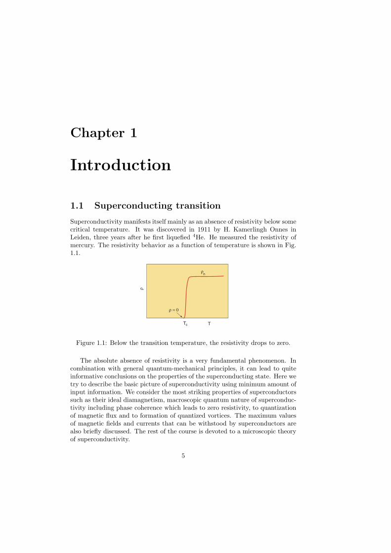
Superconductivity manifests itself mainly as an absence of resistivity below somecritical temperature. It was discovered in 1911 by H. Kamerlingh Onnes inLeiden, three years after he first liquefied 4He. He measured the resistivity ofmercury. The resistivity behavior as a function of temperature is shown in Fig.1.1.
ρ
TTc
ρn
ρ = 0
Figure 1.1: Below the transition temperature, the resistivity drops to zero.
The absolute absence of resistivity is a very fundamental phenomenon. Incombination with general quantum-mechanical principles, it can lead to quiteinformative conclusions on the properties of the superconducting state. Here wetry to describe the basic picture of superconductivity using minimum amount ofinput information. We consider the most striking properties of superconductorssuch as their ideal diamagnetism, macroscopic quantum nature of superconduc-tivity including phase coherence which leads to zero resistivity, to quantizationof magnetic flux and to formation of quantized vortices. The maximum valuesof magnetic fields and currents that can be withstood by superconductors arealso briefly discussed. The rest of the course is devoted to a microscopic theoryof superconductivity.
5

6 CHAPTER 1. INTRODUCTION
Table 1.1: Parameters for metallic superconductors
Tc, K Hc, Oe Hc2, Oe λL, A ξ0, A κ TypeAl 1.18 105 500 16000 0.01 IHg 4.15 400 400 INb 9.25 1600 2700 470 390 1.2 IIPb 7.2 800 390 830 0.47 ISn 3.7 305 510 2300 0.15 IIn 3.4 300 400 3000 IV 5.3 1020 400 ∼300 ∼ 0.7 II
Table 1.2: Parameters for some high temperature superconductors
Tc, K Hc2, T λL, A ξ0, A κ TypeNb3Sn 18 25 ∼2000 115 IILa0.925Sr0.072CuO4 34 1500 20 75 IIYBa2Cu3O7 92.4 150 2000 15 140 IIBi2Sr2Ca3CuO10 111 IITl2Sr2Ca2Cu3O10 123 IIHgBa2Ca2Cu3O8 133 IIMgB2 36.7 14 1850 50 40 II

1.2. THE LONDON MODEL 7
1.2 The London model
We assume that the current flows without dissipation and has the form
js = nsevs
whence the velocity of superconducting electrons is vs = j/nse where ns istheir density. Now we come to the most important argument [F. London andH. London, 1935]: Being non-dissipative, this current contributes to the kineticenergy of superconducting electrons. The total free energy is a sum of the kineticenergy of superconducting electrons and the magnetic energy
F =∫ [
nsmv2s
2+
h2
8π
]dV =
∫ [mj2s
2nse2+
h2
8π
]dV .
Here h is the “microscopic” magnetic field. Its average over large area in thesample gives the magnetic induction B. Using the Maxwell equation
js = (c/4π)curlh , (1.1)
we transform this to the following form
F =∫ [
mc2
32π2nse2(curlh)2 +
h2
8π
]dV =
18π
∫dV
[h2 + λ2
L (curlh)2]. (1.2)
Here
λL =(
mc2
4πnse2
) 12
(1.3)
is called the London penetration depth. In equilibrium, the free energy is min-imal with respect to distribution of the magnetic field. Variation with respectto h gives
δF =14π
∫dV
[h · δh + λ2
L (∇× h) · (∇× δh)]
=14π
∫dV
(h + λ2
L∇×∇× h)· δh +
14π
∫dV div [δh × curlh] .
Here we use the identity
div [b × a] = a · [∇× b] − b · [∇× a]
and put a = ∇× h, b = δh. Looking for a free energy minimum and omittingthe surface term we obtain the London equation:
h + λ2Lcurl curlh = 0 . (1.4)
Sincecurl curlh = ∇div h −∇2h
and div h = 0, we findh − λ2
L∇2h = 0 . (1.5)

8 CHAPTER 1. INTRODUCTION
h
hy
x0
S
λL
Figure 1.2: The Meissner effect: Magnetic field penetrates into a superconductoronly over distances shorter than λL.
1.2.1 Meissner effect
Equation (1.5) in particular describes the Meissner effect, i.e., an exponentialdecay of weak magnetic fields and supercurrents in a superconductor. Thecharacteristic length over which the magnetic field decreases is just λL. Considera superconductor which occupies the half-space x > 0. A magnetic field hy isapplied parallel to its surface (Fig. 1.2). We obtain from Eq. (1.5)
∂2hy
∂x2− λ−2
L hy = 0
which gives
hy = hy(0) exp(−x/λ) .
The field decays in a superconductor such that there is no field in the bulk.According to Eq. (1.1) the supercurrent also decays and vanishes in the bulk.
Therefore,
B = H + 4πM = 0
in a bulk superconductor, where H is the applied filed. The magnetization andsusceptibility are
M = − H4π
; χ =∂M
∂H= − 1
4π(1.6)
as for an ideal diamagnetic: Superconductor repels magnetic field lines. TheMeissner effect in type I superconductors persists up to the field H = Hc (seeTable 1.1, Fig. 1.7, and the section below) above which superconductivity isdestroyed. Type II superconductors display the Meissner effect up to muchlower fields, after which vortices appear (see Section 1.5).
1.3. PHASE COHERENCE 9
1.3 Phase coherence
The particle mass flow is determined by the usual quantum-mechanical expres-sion for the momentum per unit volume
jm = − ih2
[ψ∗∇ψ − ψ∇ψ∗] = h |ψ|2 ∇χ . (1.7)
In order to have a finite current in the superconductor it is necessary that ψis the wave function of all the superconducting electrons with a definite phase χ:the superconducting electrons should all be in a single quantum state. Accordingto the present understanding what happens is that the electrons (Fermi parti-cles) combine into pairs (Cooper pairs, see the next Chapter) which are Boseobjects and condense into a Bose condensate. The current appears when thephase χ of the condensate function ψ slowly varies in space. Equation (1.7) sug-gests that P = h∇χ is the momentum of a condensate particle (which is a pair inthe superconductor). For charged particles, the momentum is p = P− (e∗/c)Awhere P is the canonical momentum, A is the vector potential of the magneticfield, and e∗ is the charge of the carrier. In superconductors the charge is carriedby pairs of electrons thus e∗ = 2e and the Cooper pair mass is 2m.
Using the definition of the momentum we introduce the velocity of super-conducting electrons
vs =h
2m
(∇χ− 2e
hcA). (1.8)
Now the electric current becomes
js = nsevs = −e2ns
mc
(A − hc
2e∇χ). (1.9)
where |ψ|2 = ns/2 is the density of electron pairs.It is instructive to compare this equation with Eqs. (1.1) and (1.4). We find
from these
curl j =c
4πcurl curlh = − c
4πλ2L
h = − c
4πλ2L
curlA
Therefore,
j = − c
4πλ2L
(A −∇φ) = −e2ns
mc(A −∇φ)
where ∇φ is a gradient of some function. It is seen that this coincides with Eq.(1.9) where φ = (hc/2e)χ.
1.3.1 Magnetic flux quantization
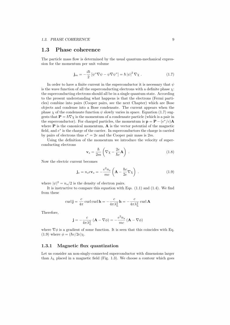
Let us consider an non-singly-connected superconductor with dimensions largerthan λL placed in a magnetic field (Fig. 1.3). We choose a contour which goes

10 CHAPTER 1. INTRODUCTION
B
l
Figure 1.3: Magnetic flux through the hole in a superconductor is quantized.
all the way inside the superconductor around the hole and calculate the contourintegral∮ (
A − hc
2e∇χ)· dl =
∫S
curlA · dS − hc
2eΔχ = Φ − hc
2e2πn . (1.10)
Here Φ is the magnetic flux through the contour. The phase change along theclosed contour is Δχ = 2πn where n is an integer because the wave function ψis single valued. Since j = 0 in the bulk, the l.h.s. of Eq. (1.10) vanishes, andwe obtain Φ = Φ0n where
Φ0 =πhc
e≈ 2.07 · 10−7 Oe · cm2 (1.11)
is the quantum of magnetic flux. In SI units, Φ0 = πh/e.
1.3.2 Coherence length and the energy gap
Cooper pairs keep their correlation within a certain distance called the coher-ence length ξ (see the next Chapter). This length introduces an importantenergy scale. To see this let us argue as follows. Since the correlation of pairsis restricted within ξ the phase gradient ∇χ cannot exceed 1/ξ; thus the super-conducting velocity cannot be larger than the critical value
vc =h
αmξ. (1.12)
where α ∼ 1 is a constant. Thus the energy of a correlated motion of a pair isrestricted to Δ0 ∼ pF vc = hvF /αξ. This gives
ξ ∼ hvF
Δ0.
The quantity Δ0 is in fact the value of the energy gap Δ(0) at zero temper-ature in the single-particle excitation spectrum in the superconducting state.

1.4. CRITICAL CURRENTS AND MAGNETIC FIELDS 11
We shall see from the microscopic theory in the next Chapter that the energyof excitations
ε =
√(p2
2m− EF
)2
+ Δ2
cannot be smaller than a certain value Δ that generally depends on temperature.The coherence length is usually defined as
ξ0 =hvF
2πkBTc
where Δ0 = 1.76kBTc and ξ0 is the coherence length at zero temperature of aclean (without impurities) material. In alloys with < ξ0,
ξ =√ξ0
where is the mean free path.The ratio
κ =λL
ξ
is called the Ginzburg–Landau parameter. Its magnitude separates all super-conductors between type-I (κ < 1/
√2 ≈ 0.7) and type-II (κ > 1/
√2) supercon-
ductors. For alloys with < ξ0
κ = 0.75λ0
where λ0 is the London length in a clean material at zero temperature. Theconclusion is that alloys are type-II superconductors. Values of λL, ξ0, and κfor some materials are listed in Tables 1.1 and 1.2.
1.4 Critical currents and magnetic fields
1.4.1 Condensation energy
The kinetic energy density of condensate (superconducting) electrons cannotexceed
Fc =nsmv
2c
2=
nsh2
2α2mξ2. (1.13)
If the velocity vs increases further, the kinetic energy exceeds the energy gainof the superconducting state with respect to the normal state Fn − Fs, andsuperconductivity disappears. Therefore, Fc = Fn − Fs is just this energy gainwhich is called the condensation energy.
Assume now that the superconductor is placed in a magnetic field H. Itrepels the field thus increasing the energy of the external source that createsthe field. The energy of the entire system increases and becomes
F = Fs +H2
8π= Fn − Fc +
H2
8π.
12 CHAPTER 1. INTRODUCTION
In the superconducting state, F < Fn. When the energy reaches the energy ofa normal state Fn, the superconductivity becomes no longer favorable energet-ically. Thus the thermodynamic critical magnetic field satisfies
Fc =H2
c
8π.
Using the expression for λL we find from Eq.(1.13)
Hc =hc
αeλLξ=
Φ0
απλLξ
The exact expression for Hc at temperatures close to Tc is
Hc =Φ0
2√
2πλLξ(1.14)
Values of Hc for some materials are given in Table 1.1.
1.4.2 Critical currents
There may be several mechanisms of destruction of superconductivity by a cur-rent flowing through it.
Mechanism 1. Large type-I samples: The critical current Ic creates Hc atthe sample surface. For a cylinder with a radius R,
2πRHc =4πcIc .
If R � λL, the current flows only within the layer of a thickness λL near thesample surface. Thus Ic = 2πRλLjc and
jc =cHc
4πλL. (1.15)
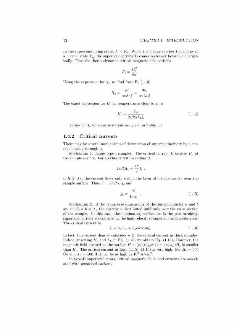
Mechanism 2. If the transverse dimensions of the superconductor a and bare small, a, b � λL the current is distributed uniformly over the cross sectionof the sample. In this case, the dominating mechanism is the pair-breaking:superconductivity is destroyed by the high velocity of superconducting electrons.The critical current is
jc = nsevc = nseh/αmξ . (1.16)
In fact, this current density coincides with the critical current in thick samples.Indeed, inserting Hc and λL in Eq. (1.15) we obtain Eq. (1.16). However, themagnetic field created at the surface H ∼ (c/4π)jca2/a ∼ (a/λL)Hc is smallerthan Hc. The critical current in Eqs. (1.15), (1.16) is very high. For Hc = 500Oe and λL = 500 A it can be as high as 108 A/cm2.
In type-II superconductors, critical magnetic fields and currents are associ-ated with quantized vortices.

1.5. QUANTIZED VORTICES 13
B
Figure 1.4: Singular lines in a SC with 2πn phase variations around them.
1.5 Quantized vortices
1.5.1 Basic concepts
Consider a type-II superconductor where the London length is large. The super-current and magnetic field do not vanish within the region of the order of λ fromthe surface: there exists a sizable region of nonzero vs. If the magnetic field islarge enough, vs can reach high values, vs ∼ (e/mc)Hr. For fields H ∼ hc/eξ2,the velocity can reach rh/mξ2 � vc for r � ξ. This would lead to destruction ofsuperconductivity if there were no means for compensating a large contributionto vs due to the magnetic field.
Assume that we have a linear singularity such that the phase χ of the wavefunction of superconducting electrons ψ changes by 2πn if one goes around thislines along a closed contour, see Fig. 1.4. Consider again the integral along thiscontour
−mce
∮vs · dl =
∮ (A − hc
2e∇χ)· dl =
∫S
curlA · dS − hc
2eΔχ
= Φ − hc
2e2πn = Φ − Φ0n . (1.17)
Here Φ is the magnetic flux through the contour, Φ0 is the flux quantum. Thephase change along the closed contour is Δχ = 2πn. We observe that the super-conducting velocity increase is completely compensated by the phase variationif the magnetic flux is Φ = Φ0n. One can thus expect that in superconductorswith large λL in high magnetic fields, there will appear linear singularities witha surface density nL such that (Φ0n)nL is equal to the magnetic induction B.Under these conditions, the superconducting velocity does not increase withdistance, and superconductivity is conserved on average.
Each singularity of the phase can exist if the wave function of the supercon-ducting electrons, i.e., the density of superconducting electrons ns = 2|ψ|2 goesto zero at the singular line. The size of the region where ns is decreased with
14 CHAPTER 1. INTRODUCTION
respect to its equilibrium value has a size of the order of the coherence length ξand is called the vortex core. Such singular objects are called quantized vortices:each vortex carries a quantized magnetic flux Φ0n. The condition required forexistence of vortices is λ > ξ or exactly κ > 1/
√2. More favorable energetically
are singly quantized vortices which carry one magnetic flux quantum and havea phase circulation 2π around the vortex axis.
Vortices are the objects which play a very special role in superconductors andsuperfluids. In superconductors, each vortex carries exactly one magnetic-fluxquantum. Being magnetically active, vortices determine the magnetic propertiesof superconductors. In addition, they are mobile if the material is homogeneous.In fact, a superconductor in the vortex state is no longer superconducting in ausual sense. Indeed, there is no complete Meissner effect: some magnetic fieldpenetrates into the superconductor via vortices. In addition, regions with thenormal phase appear: since the order parameter turns to zero at the vortex axisand is suppressed around each vortex axis within a vortex core with a radiusof the order of the coherence length, there are regions with a finite low-energydensity of states. Moreover, mobile vortices come into motion in the presenceof an average (transport) current. This produces dissipation and causes a finiteresistivity (the so-called flux flow resistivity): a superconductor is no longer“superconducting”.
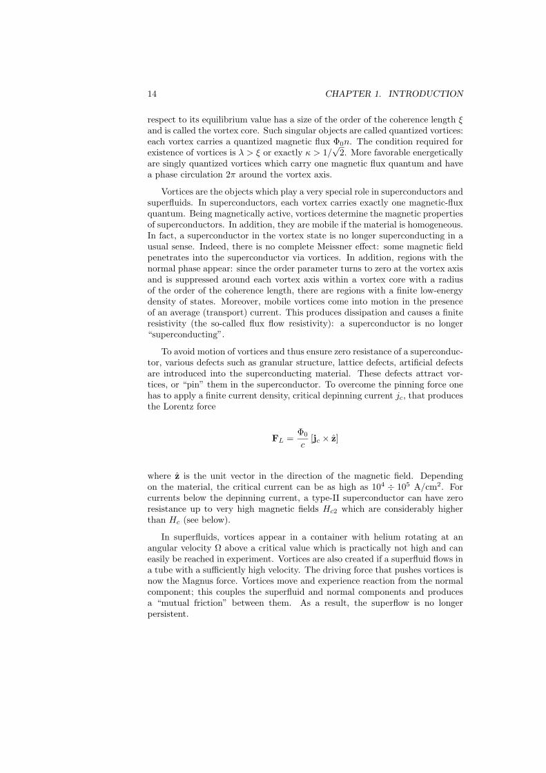
To avoid motion of vortices and thus ensure zero resistance of a superconduc-tor, various defects such as granular structure, lattice defects, artificial defectsare introduced into the superconducting material. These defects attract vor-tices, or “pin” them in the superconductor. To overcome the pinning force onehas to apply a finite current density, critical depinning current jc, that producesthe Lorentz force
FL =Φ0
c[jc × z]
where z is the unit vector in the direction of the magnetic field. Dependingon the material, the critical current can be as high as 104 ÷ 105 A/cm2. Forcurrents below the depinning current, a type-II superconductor can have zeroresistance up to very high magnetic fields Hc2 which are considerably higherthan Hc (see below).
In superfluids, vortices appear in a container with helium rotating at anangular velocity Ω above a critical value which is practically not high and caneasily be reached in experiment. Vortices are also created if a superfluid flows ina tube with a sufficiently high velocity. The driving force that pushes vortices isnow the Magnus force. Vortices move and experience reaction from the normalcomponent; this couples the superfluid and normal components and producesa “mutual friction” between them. As a result, the superflow is no longerpersistent.

1.5. QUANTIZED VORTICES 15
1.5.2 Vortices in the London model
Let us take curl of Eq. (1.9). We find
h − hc
2ecurl∇χ = − mc
nse2curl js = −λ2
Lcurl curlh .
This looks like Eq. (1.5) except for one extra term. This term is nonzero ifthere are vortices. In the presence of vortices, the London equation should bemodified. For an n-quantum vortex we have
curl∇χ = 2πnzδ(2)(r)
where z is the unit vector in the direction of the vortex axis. Therefore, theLondon equation for a vortex becomes
h + λ2Lcurl curlh = nΦ0δ
(2)(r) (1.18)
where Φ0 is the vector along the vortex axis with the magnitude of one fluxquantum. For a system of vortices
h + λ2Lcurl curlh = nΦ0
∑k
δ(2)(r − rk) (1.19)
where the sum is over all the vortex positions rk.One can easily find the magnetic field for a single straight vortex (see Prob-
lem 1.1). In cylindrical coordinates h = (0, 0, hz(r)), the magnetic field is
hz(r) =nΦ0
2πλ2L
ln(λL
r
)
near the vortex axis r � λL. The magnetic field increases logarithmically nearthe vortex axis. However, in our model, the coordinate r cannot be made shorterthan the coherence length since ns vanishes at the vortex axis, and the Londonequation does not apply for r < ξ. Therefore, at the axis
h(0) =nΦ0
2πλ2L
ln(λL
ξ
).
We can calculate the current around the vortex near the core.
jφ =c
4π∂hz
∂r=
ncΦ0
8π2λ2Lr
=nsenh
2mr
For a single-quantum vortex the superconducting velocity is
vs,φ =h
2mr
Therefore, the phase is just the azimuthal angle:
χ = φ
16 CHAPTER 1. INTRODUCTION
h
⏐ψ⏐=ns1/2
ξ λ rL
js
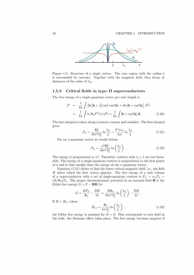
Figure 1.5: Structure of a single vortex. The core region with the radius ξis surrounded by currents. Together with the magnetic field, they decay atdistances of the order of λL.
1.5.3 Critical fields in type–II superconductors
The free energy of a single-quantum vortex per unit length is
F =18π
∫ [h(h + λ2
Lcurl curlh)
+ div[h × curlh]]d2r
=18π
∫hzΦ0δ
(2)(r) d2r +18π
∫[h × curlh] dl . (1.20)
The last integral is taken along a remote contour and vanishes. The first integralgives
FL =Φ2
0
16π2λ2L
lnλL
ξ=h2πns
4mlnλL
ξ. (1.21)
For an n-quantum vortex we would obtain
FL =n2Φ2
0
16π2λ2L
ln(λL
ξ
). (1.22)
The energy is proportional to n2. Therefore, vortices with n > 1 are not favor-able: The energy of n single-quantum vortices is proportional to the first powerof n and is thus smaller than the energy of one n-quantum vortex.
Equation (1.21) allows to find the lower critical magnetic field, i.e., the fieldH above which the first vortex appears. The free energy of a unit volumeof a superconductor with a set of single-quantum vortices is FL = nLFL =(B/Φ0)FL. The proper thermodynamic potential in an external field H is theGibbs free energy G = F − HB/4π
G =BFL
Φ0− BH
4π=
BΦ0
16π2λ2L
ln(λL
ξ
)− BH
4π.
If H < Hc1 where
Hc1 =Φ0
4πλ2L
ln(λL
ξ
), (1.23)
the Gibbs free energy is minimal for B = 0. This corresponds to zero field inthe bulk: the Meissner effect takes place. The free energy becomes negative if
1.5. QUANTIZED VORTICES 17
Meissner
VortexNormal
H
T T
HH
H
c
c
c1
c2
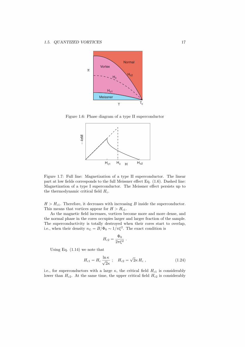
Figure 1.6: Phase diagram of a type II superconductor
− 4π
M
H Hc1 c2HHc
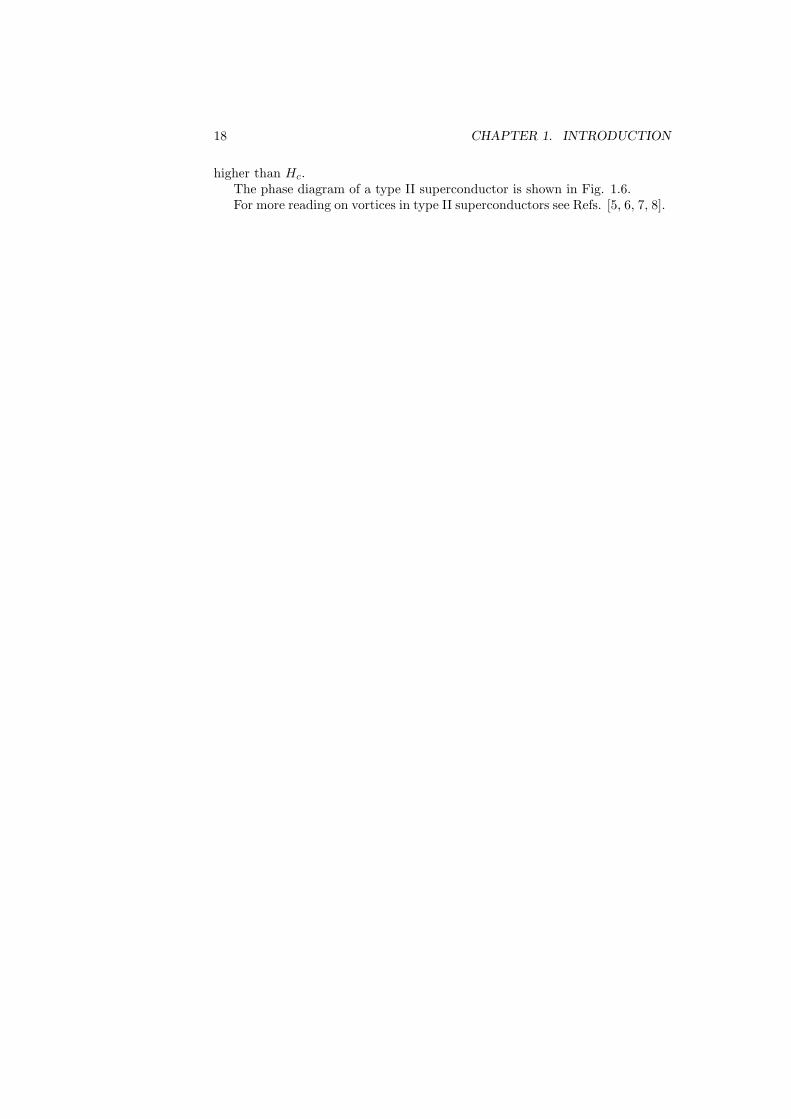
Figure 1.7: Full line: Magnetization of a type II superconductor. The linearpart at low fields corresponds to the full Meissner effect Eq. (1.6). Dashed line:Magnetization of a type I superconductor. The Meissner effect persists up tothe thermodynamic critical field Hc.
H > Hc1. Therefore, it decreases with increasing B inside the superconductor.This means that vortices appear for H > Hc1.
As the magnetic field increases, vortices become more and more dense, andthe normal phase in the cores occupies larger and larger fraction of the sample.The superconductivity is totally destroyed when their cores start to overlap,i.e., when their density nL = B/Φ0 ∼ 1/πξ2. The exact condition is
Hc2 =Φ0
2πξ2.
Using Eq. (1.14) we note that
Hc1 = Hclnκ√
2κ; Hc2 =
√2κHc , (1.24)
i.e., for superconductors with a large κ, the critical field Hc1 is considerablylower than Hc2. At the same time, the upper critical field Hc2 is considerably
18 CHAPTER 1. INTRODUCTION
higher than Hc.The phase diagram of a type II superconductor is shown in Fig. 1.6.For more reading on vortices in type II superconductors see Refs. [5, 6, 7, 8].
Chapter 2
The BCS theory
2.1 Landau Fermi-liquid
The ground state of a system of Fermions corresponds to the filled states withenergies E below the maximal Fermi energy EF , determined by the numberof Fermions. In an homogeneous system, one can describe particle states bymomentum p such that the spectrum becomes Ep. The condition of maximumenergy Ep = EF defines the Fermi surface in the momentum space. In anisotropic system, this is a sphere such that its volume divided by (2πh)3
nα =4πp3
F
3(2πh)3
gives number of particles with the spin projection α per unit (spatial) volumeof system. For electrons with spin 1
2 , the total number of particles in the unitvolume of the system, i.e., the particle density is twice nα
n =p3
F
3π2h3 (2.1)
This ground state corresponds to a ground-state energy E0.Excitations in the Fermi liquid that increase its energy as compared to E0
are created by moving a particle from a state below the Fermi surface to a stateabove it. This process can be considered as a superposition of two processes.First is a removal of a particle from the system out of a state below the Fermisurface. The second is adding a particle to a state above the Fermi surface. Bytaking a particle out of the state with an energy E1 < EF we increase the energyof the system and create a hole excitation with a positive energy ε1 = EF −E1.By adding a particle into a state with an energy E2 > EF we again increase theenergy and create a particle excitation with a positive energy ε2 = E2 − EF .The energy of the system is thus increased by ε1 + ε2 = E2 − E1.
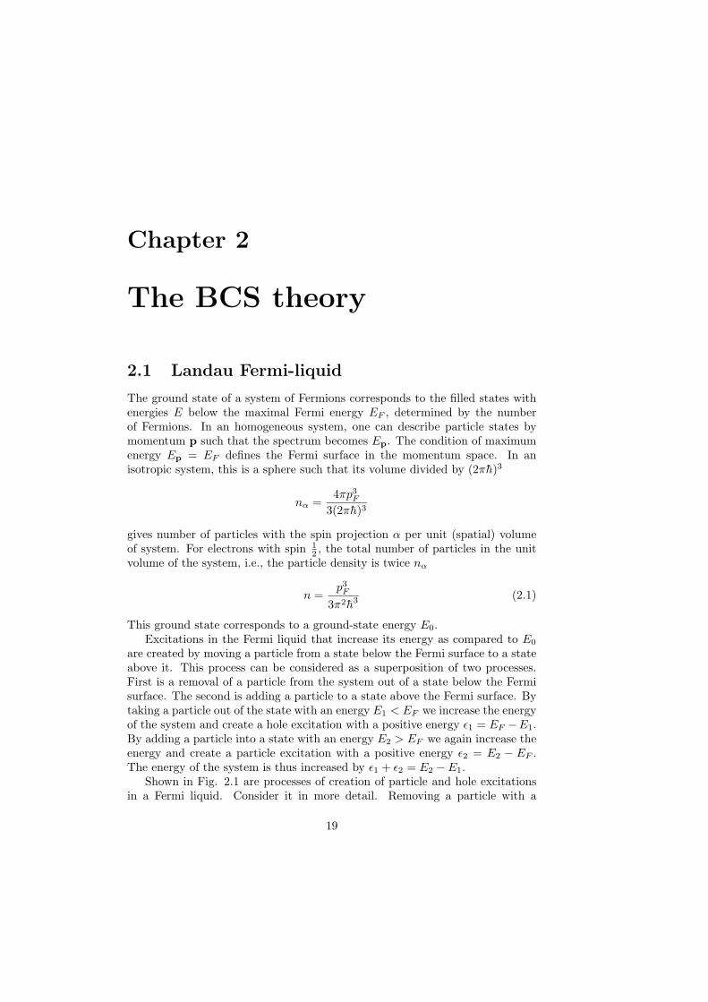
Shown in Fig. 2.1 are processes of creation of particle and hole excitationsin a Fermi liquid. Consider it in more detail. Removing a particle with a
19
20 CHAPTER 2. THE BCS THEORY
p-p'
Fp
p'
Figure 2.1: Particle (shaded circle) and hole (white circle) excitations in LandauFermi liquid. The particle excitation is obtained by adding a particle. The holeexcitation is obtained by removing a particle (black circle) with an oppositemomentum.
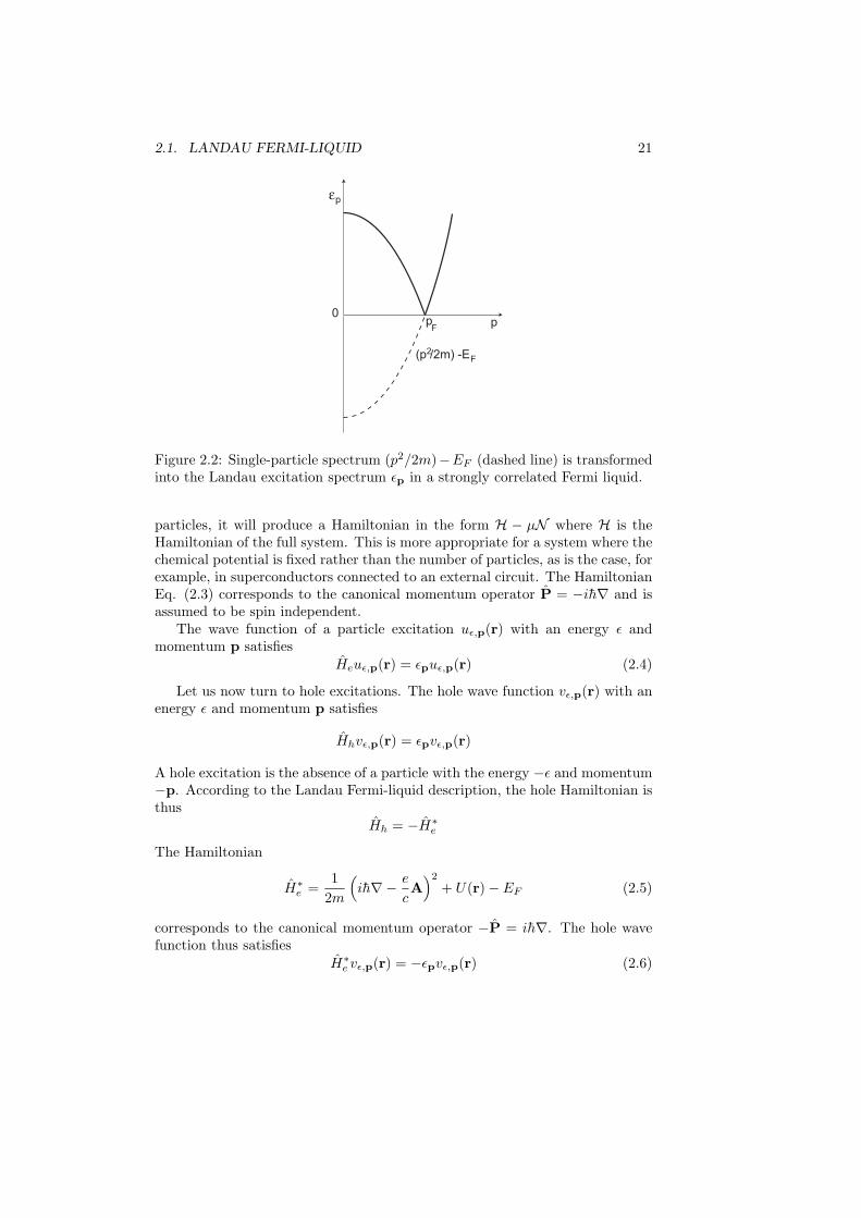
momentum p′ and an energy E′ from below the Fermi surface, p′ < pF andE′ < EF , creates an excitation with a momentum −p′ and an energy ε−p′ =EF −E′. Adding a particle with a momentum p and energy E above the Fermisurface, p > pF and E > EF , creates an excitation with momentum p andenergy εp = E−EF . For an isotropic system, the excitation spectrum will thushave the form
εp =
{p2
2m − EF , p > pF
EF − p2
2m , p < pF
(2.2)
shown in Fig. 2.2.The particle and hole excitations live in a system of Fermions where a strong
correlation exists due to the Pauli principle. How well elementary excitationswith a free-particle spectrum Eq. (2.2) are defined here?
One can show that uncertainty of the quasiparticle energy due to quasiparticle-quasiparticle scattering, δε ∼ hP , where P is the probability of scattering, in2 dimensional and 3 dimensional systems is small compared to the energy ifε � EF , i.e., near the Fermi surface. In other words, quasiparticles are welldefined only near the Fermi surface. For a one dimensional system, however,the sirtuation is different, and the Landau quasiparticles do not exist. Theone-dimensional system of Fermions is known as the Luttinger liquid, which isbeyond the present course.
Let us now define the Hamiltonian for particles and holes. For particles, wedefine a single-electron Hamiltonian
He =1
2m
(−ih∇− e
cA)2
+ U(r) − μ (2.3)
where μ is the chemical potential and U(r) is some potential energy. In thenormal state, μ = EF . Being applied to a system of totally N =
∫ndV
2.1. LANDAU FERMI-LIQUID 21
(p /2m) -E2F
εp
0pp
F
Figure 2.2: Single-particle spectrum (p2/2m)−EF (dashed line) is transformedinto the Landau excitation spectrum εp in a strongly correlated Fermi liquid.
particles, it will produce a Hamiltonian in the form H − μN where H is theHamiltonian of the full system. This is more appropriate for a system where thechemical potential is fixed rather than the number of particles, as is the case, forexample, in superconductors connected to an external circuit. The HamiltonianEq. (2.3) corresponds to the canonical momentum operator P = −ih∇ and isassumed to be spin independent.
The wave function of a particle excitation uε,p(r) with an energy ε andmomentum p satisfies
Heuε,p(r) = εpuε,p(r) (2.4)
Let us now turn to hole excitations. The hole wave function vε,p(r) with anenergy ε and momentum p satisfies
Hhvε,p(r) = εpvε,p(r)
A hole excitation is the absence of a particle with the energy −ε and momentum−p. According to the Landau Fermi-liquid description, the hole Hamiltonian isthus
Hh = −H∗e
The Hamiltonian
H∗e =
12m
(ih∇− e
cA)2
+ U(r) − EF (2.5)
corresponds to the canonical momentum operator −P = ih∇. The hole wavefunction thus satisfies
H∗e vε,p(r) = −εpvε,p(r) (2.6)
22 CHAPTER 2. THE BCS THEORY
p'
-p'
p
pF
-p
p
pF
(a) (b)
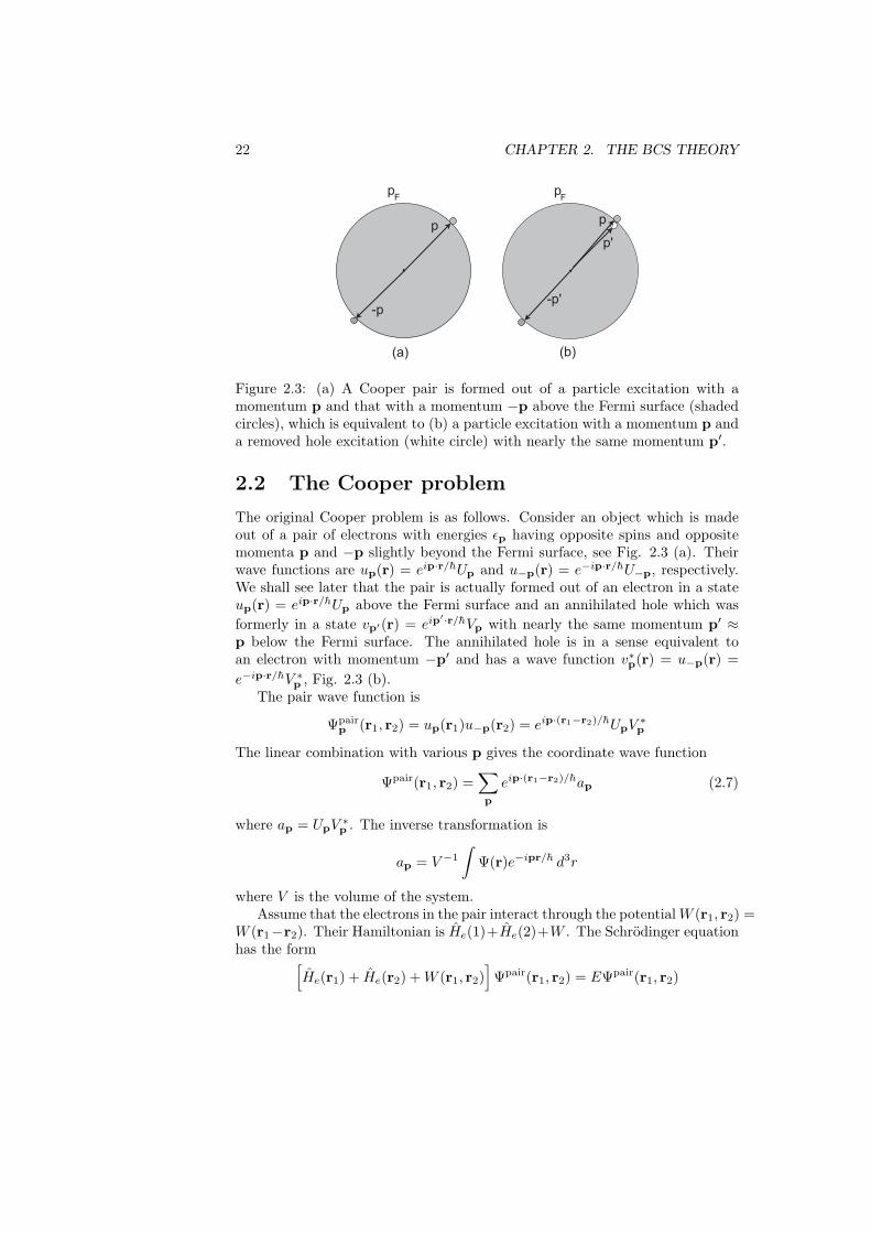
Figure 2.3: (a) A Cooper pair is formed out of a particle excitation with amomentum p and that with a momentum −p above the Fermi surface (shadedcircles), which is equivalent to (b) a particle excitation with a momentum p anda removed hole excitation (white circle) with nearly the same momentum p′.
2.2 The Cooper problem
The original Cooper problem is as follows. Consider an object which is madeout of a pair of electrons with energies εp having opposite spins and oppositemomenta p and −p slightly beyond the Fermi surface, see Fig. 2.3 (a). Theirwave functions are up(r) = eip·r/hUp and u−p(r) = e−ip·r/hU−p, respectively.We shall see later that the pair is actually formed out of an electron in a stateup(r) = eip·r/hUp above the Fermi surface and an annihilated hole which wasformerly in a state vp′(r) = eip′·r/hVp with nearly the same momentum p′ ≈p below the Fermi surface. The annihilated hole is in a sense equivalent toan electron with momentum −p′ and has a wave function v∗p(r) = u−p(r) =e−ip·r/hV ∗
p , Fig. 2.3 (b).The pair wave function is
Ψpairp (r1, r2) = up(r1)u−p(r2) = eip·(r1−r2)/hUpV
∗p
The linear combination with various p gives the coordinate wave function
Ψpair(r1, r2) =∑p
eip·(r1−r2)/hap (2.7)
where ap = UpV∗p . The inverse transformation is
ap = V −1
∫Ψ(r)e−ipr/h d3r
where V is the volume of the system.Assume that the electrons in the pair interact through the potentialW (r1, r2) =
W (r1−r2). Their Hamiltonian is He(1)+He(2)+W . The Schrodinger equationhas the form[
He(r1) + He(r2) +W (r1, r2)]Ψpair(r1, r2) = EΨpair(r1, r2)

2.2. THE COOPER PROBLEM 23
Multiplying this by e−ip(r1−r2) and calculating the integral over the volume weobtain this equation in the momentum representation,
[2εp − Ep] ap = −∑p1
Wp,p1ap1
whereWp,p1 = V −1
∫e−i(p−p1)·r/hW (r) d3r
Assume that
Wp,p1 ={W/V, εp and εp1 < Ec
0, εp or εp1 > Ec
where Ec � EF . The interaction strength W ∼ W0v0 where W0 is the magni-tude of the interaction potential while v0 = a3
0 is the volume where the interac-tion of a range a0 is concentrated. We have
ap =W
E − 2εp1V
∑p1
ap1 =W
E − 2εp
∑p1
′ap1 (2.8)
Here the sum∑
p is taken over p which satisfy εp < Ec, while the sum∑′ is
taken over the states in a unit volume. Let us denote
C =∑p
′ap
Eq. (2.8) yields
ap =WC
E − 2εpwhence
C = WC∑p
′ 1E − 2εp
This gives1W
=∑p
′ 1E − 2εp
≡ Φ(E) (2.9)
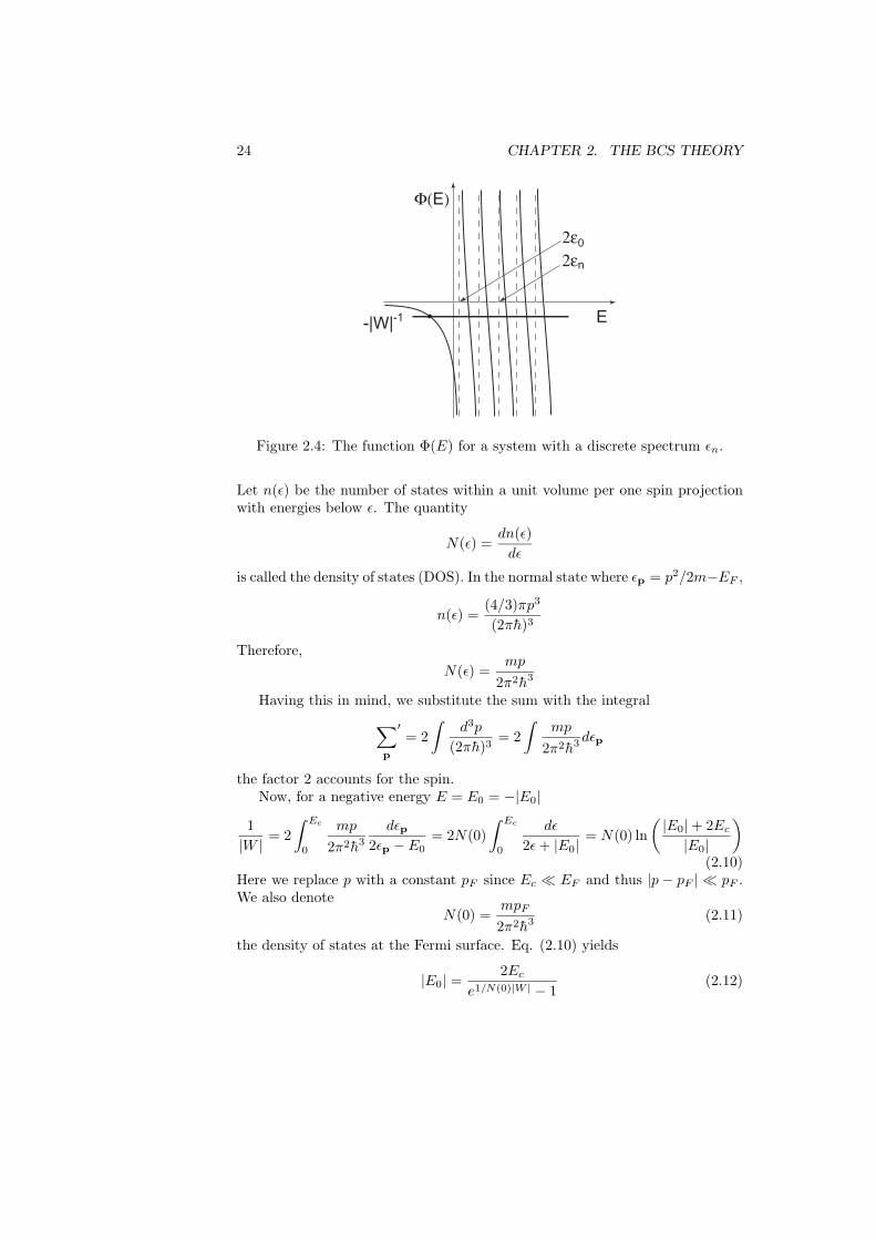
Equation (2.9) is illustrated in Fig. 2.4. Let us put our system in a largebox. The levels εp will become a discrete set εn shown in Fig. 2.4 by verticaldashed lines. The lowest level ε0 is very close to zero and will approach zero asthe size of the box increases. The function Φ(E) varies from −∞ to +∞ as Eincreases and crosses each εn > 0. However, for negative E < 0, the functionΦ(E) approaches zero as E → −∞, and there is a crossing point with a negativelevel −1/|W | for negative E. This implies that there is a state with negativeenergy E0 < 0 satisfying Eq. (2.9) for a negative W < 0.
For an attraction W < 0 we have
1|W | =
∑p
′ 12εp − E
24 CHAPTER 2. THE BCS THEORY
Φ(E)
E-|W|-1
2εn2ε0
Figure 2.4: The function Φ(E) for a system with a discrete spectrum εn.
Let n(ε) be the number of states within a unit volume per one spin projectionwith energies below ε. The quantity
N(ε) =dn(ε)dε
is called the density of states (DOS). In the normal state where εp = p2/2m−EF ,
n(ε) =(4/3)πp3
(2πh)3
Therefore,N(ε) =
mp
2π2h3
Having this in mind, we substitute the sum with the integral
∑p
′= 2
∫d3p
(2πh)3= 2
∫mp
2π2h3 dεp
the factor 2 accounts for the spin.Now, for a negative energy E = E0 = −|E0|
1|W | = 2
∫ Ec
0
mp
2π2h3
dεp2εp − E0
= 2N(0)∫ Ec
0
dε
2ε+ |E0|= N(0) ln
(|E0| + 2Ec
|E0|
)(2.10)
Here we replace p with a constant pF since Ec � EF and thus |p− pF | � pF .We also denote
N(0) =mpF
2π2h3 (2.11)
the density of states at the Fermi surface. Eq. (2.10) yields
|E0| =2Ec
e1/N(0)|W | − 1(2.12)
2.2. THE COOPER PROBLEM 25
The dimensionless factor λ ≡ N(0)W ∼ N(0)W0a30 is called the interaction
constant. For weak coupling, N(0)|W | � 1, we find
|E0| = 2Ece−1/N(0)|W |
For a strong coupling, N(0)|W | � 1,
|E0| = 2N(0)|W |Ec
We see that there exists a state of a particle-hole pair (the Cooper pair) withan energy |E0| below the Fermi surface. It means that the system of normal-state particles and holes is unstable towards formation of pairs provided thereis an attraction (however small) between electrons: Indeed, if we place a pair ofextra electrons in a system which has a filled Fermi surface, these two electronsfind a state below the Fermi surface, in contradiction to the assumption thatthere are no more available states inside the Fermi surface.
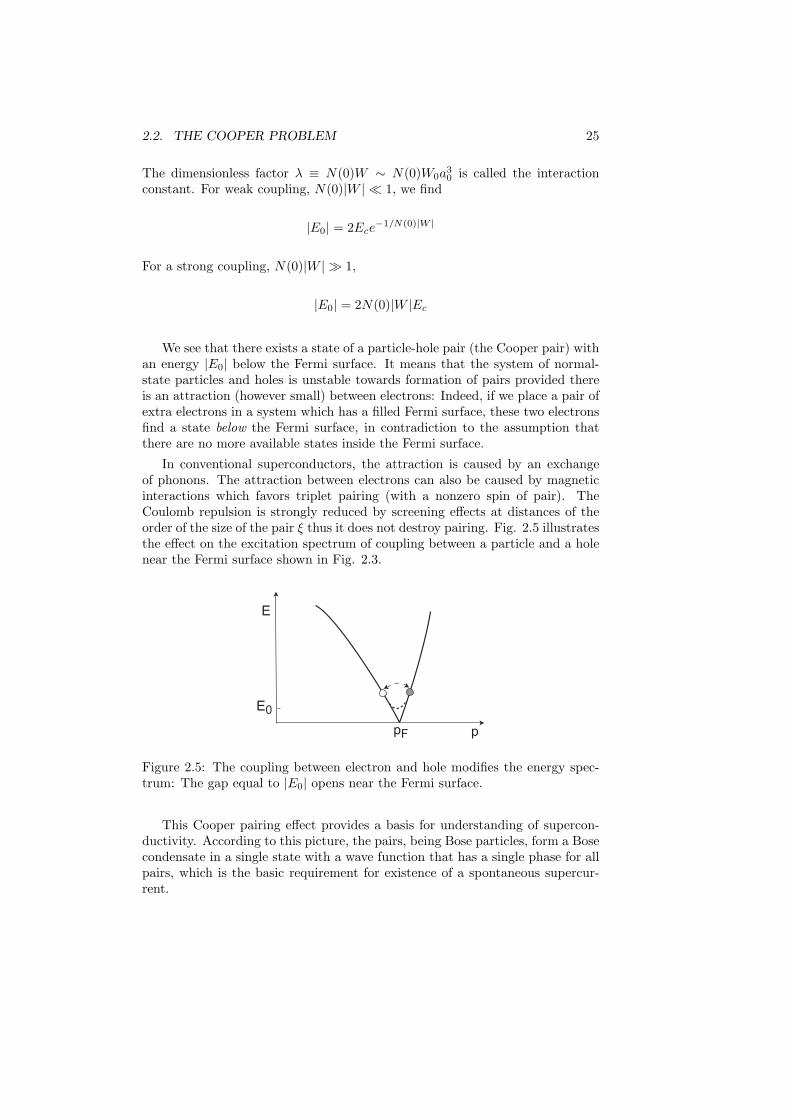
In conventional superconductors, the attraction is caused by an exchangeof phonons. The attraction between electrons can also be caused by magneticinteractions which favors triplet pairing (with a nonzero spin of pair). TheCoulomb repulsion is strongly reduced by screening effects at distances of theorder of the size of the pair ξ thus it does not destroy pairing. Fig. 2.5 illustratesthe effect on the excitation spectrum of coupling between a particle and a holenear the Fermi surface shown in Fig. 2.3.
E
E0
pF p
Figure 2.5: The coupling between electron and hole modifies the energy spec-trum: The gap equal to |E0| opens near the Fermi surface.
This Cooper pairing effect provides a basis for understanding of supercon-ductivity. According to this picture, the pairs, being Bose particles, form a Bosecondensate in a single state with a wave function that has a single phase for allpairs, which is the basic requirement for existence of a spontaneous supercur-rent.
26 CHAPTER 2. THE BCS THEORY
2.3 The BCS model
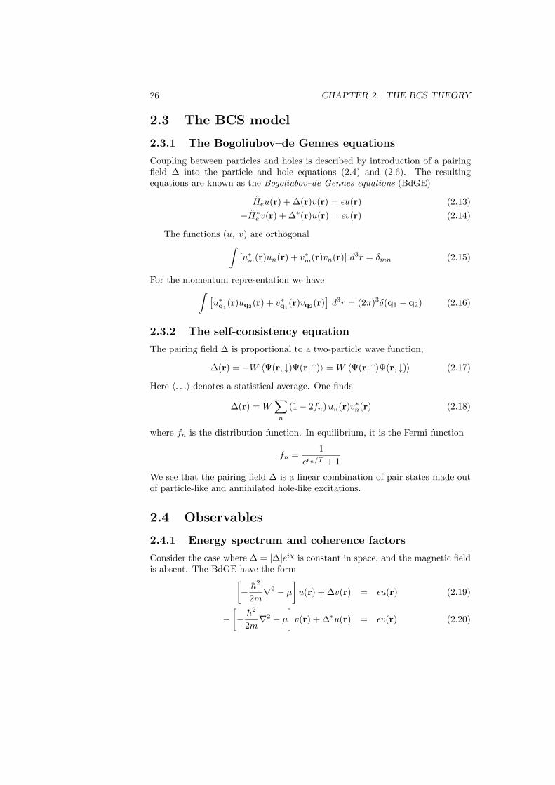
2.3.1 The Bogoliubov–de Gennes equations
Coupling between particles and holes is described by introduction of a pairingfield Δ into the particle and hole equations (2.4) and (2.6). The resultingequations are known as the Bogoliubov–de Gennes equations (BdGE)
Heu(r) + Δ(r)v(r) = εu(r) (2.13)−H∗
e v(r) + Δ∗(r)u(r) = εv(r) (2.14)
The functions (u, v) are orthogonal∫[u∗m(r)un(r) + v∗m(r)vn(r)] d3r = δmn (2.15)
For the momentum representation we have∫ [u∗q1
(r)uq2(r) + v∗q1(r)vq2(r)
]d3r = (2π)3δ(q1 − q2) (2.16)
2.3.2 The self-consistency equation
The pairing field Δ is proportional to a two-particle wave function,
Δ(r) = −W 〈Ψ(r, ↓)Ψ(r, ↑)〉 = W 〈Ψ(r, ↑)Ψ(r, ↓)〉 (2.17)
Here 〈. . .〉 denotes a statistical average. One finds
Δ(r) = W∑
n
(1 − 2fn)un(r)v∗n(r) (2.18)
where fn is the distribution function. In equilibrium, it is the Fermi function
fn =1
eεn/T + 1
We see that the pairing field Δ is a linear combination of pair states made outof particle-like and annihilated hole-like excitations.
2.4 Observables
2.4.1 Energy spectrum and coherence factors
Consider the case where Δ = |Δ|eiχ is constant in space, and the magnetic fieldis absent. The BdGE have the form[
− h2
2m∇2 − μ
]u(r) + Δv(r) = εu(r) (2.19)
−[− h2
2m∇2 − μ
]v(r) + Δ∗u(r) = εv(r) (2.20)

2.4. OBSERVABLES 27
where μ = h2k2F /2m. We look for a solution in the form
u = ei2 χUqe
iq·r , v = e−i2 χVqe
iq·r (2.21)
where q is a constant vector. We have
ξqUq + |Δ|Vq = εqUq (2.22)−ξqVq + |Δ|Uq = εqVq (2.23)
where
ξq =h2
2m[q2 − k2
F
]The condition of solvability of Eqs. (2.22) and (2.23) gives
εq = ±√ξ2q + |Δ|2 (2.24)
According to the Landau picture of Fermi liquid, we consider only energies ε > 0.The spectrum is shown in Fig. 2.6.
The wave functions u and v for a given momentum q are found from Eqs.(2.22), (2.24). We have
Uq =1√2
(1 +
ξqεq
)1/2
, Vq =1√2
(1 − ξq
εq
)1/2
(2.25)
Normalization is chosen to satisfy Eq. (2.16).The energy |Δ| is the lowest single-particle excitation energy in the super-
conducting state. 2|Δ| corresponds to an energy which is needed to destroythe Cooper pair. Therefore, one can identify 2|Δ| as the pairing energy asdetermined by the Cooper problem in the previous Section, |E| = 2|Δ|.
Electrons in the pair have velocity vF . Therefore, the characteristic momen-tum (in addition to pF ) associated with the pair is δp ∼ |Δ|/vF . Using theuncertainty principle, δpR ∼ h, where R has a meaning of effective “size” of aCooper pair, one finds R ∼ hvF /|Δ|. This characteristic scale sets up a veryimportant length scale called the coherence length
ξ ∼ hvF /|Δ| .
For a given energy, there are two possible values of
ξq = ±√ε2 − |Δ|2 (2.26)
that correspond respectively to particles or holes (see Fig. 2.6).The quantity
dε
d(hq)= vg

28 CHAPTER 2. THE BCS THEORY
E
p p
F
F
Δparticlesholes
ε
Figure 2.6: The BCS spectrum of excitations in a superconductor. The solidline shows the spectrum of quasiparticles near the Fermi surface where theLandau quasiparticles are well defined. At higher energies closer to EF theLandau quasiparticles are not well-defined (dotted line). The dashed line atlower energies shows the behavior of the spectrum in the normal state ε = |ξp|.
is the group velocity of excitations. One has q2 = k2F ± (2m/h2)
√ε2 − |Δ|2.
Therefore,
vg =hq
m
ξq√ξ2q + |Δ|2
= vFξq√
ξ2q + |Δ|2= ±vF
√ε2 − |Δ|2ε
(2.27)
where vF = hq/m is the velocity at the Fermi surface. We see that the groupvelocity is positive, i.e., its direction coincides with the direction of q for ex-citations outside the Fermi surface ξq > 0. As we know, these excitations areparticle-like. On the other hand, vg < 0 for excitations inside the Fermi surfaceξq < 0, which are known as hole-like excitations.
2.4.2 Density of states
Another important quantity is the density of states (DOS) N(ε) defined asfollows. Let us suppose that there are nα(q) states per spin and per unit volumefor particles with momenta up to hq. The density of states is the number ofstates within an energy interval from ε to ε+ dε, i.e.
N(ε) =dnα(q)dε
As we can see, in a superconductor, there are no excitations with energies ε <|Δ|. The DOS per one spin projection is zero for ε < |Δ|. For ε > |Δ| we have
N(ε) =12
∣∣∣∣ ddε(q3
3π2
)∣∣∣∣ = q2
2π2
∣∣∣∣ dεdq∣∣∣∣−1

2.4. OBSERVABLES 29
=mq
2π2h2
ε√ε2 − |Δ|2
≈ N(0)ε√
ε2 − |Δ|2(2.28)
HereN(0) =
mpF
2π2h3 =mkF
2π2h2
is the DOS per one spin projection in the normal state for zero energy excita-tions, i.e., at the Fermi surface. We have replaced here q with kF . Indeed, sinceΔ � EF , the magnitude of q is very close to kF for ε ∼ Δ. This fact is of acrucial importance for practical applications of the BCS theory, as we shall seein what follows.
N(ε
)/N
(0)
εΔ
1
Figure 2.7: The superconducting density of states as a function of energy.
2.4.3 The energy gap
For a state Eq. (2.21) specified by a wave vector q with Uq and Vq from Eq.(2.25) the product uv∗ becomes
uv∗ = eiχUqVq =Δ2εq
The self-consistency equation (2.18) yields
Δ = W∑q
(1 − 2fq)Δ2εq
(2.29)
We replace the sum with the integral
∑q
=∫ q=∞
q=0
d3q
(2π)3=∫ ξ=+∞
ξ=−EF
mq
2π2h2 dξq ≈ N(0)∫ +∞
−∞dξq
and notice that, in equilibrium,
1 − 2fq = tanh( εq
2T
)
30 CHAPTER 2. THE BCS THEORY
Moreover,εq dεq = ξq dξq
When ξ varies from −∞ to +∞, the energy varies from Δ to +∞ taking eachvalue twice. Therefore, the self-consistency equation takes the form
Δ = W∑q
(1 − 2fq)Δ2εq
= N(0)W∫ ∞
|Δ|
Δ√ε2 − |Δ|2
tanh( ε
2T
)dε (2.30)
The integral diverges logarithmically at large energies. In fact, the potentialof interaction does also depend on energy W = Wε in such a way that it vanishesfor high energies exceeding some limiting value Ec � EF . We assume that
Wε ={W, ε < Ec
0, ε > Ec
From Eq. (2.30) we obtain the gap equation
1 = λ
∫ Ec
|Δ|
1√ε2 − |Δ|2
tanh( ε
2T
)dε (2.31)
where the dimensionless parameter λ = N(0)W ∼ N(0)W0a3 is called the inter-
action constant. For phonon mediated electron coupling, the effective attractionworks for energies below the Debye energy ΩD. Therefore, Ec = ΩD in Eq.(2.31). This equation determines the dependence of the gap on temperature.
This equation can be used to determine the critical temperature Tc, at whichthe gap Δ vanishes. We have
1 = λ
∫ Ec
0
tanh(
ε
2Tc
)dε
ε(2.32)
This reduces to1λ
=∫ Ec/2Tc
0
tanhxx
dx (2.33)
The integral ∫ a
0
tanhxx
dx = ln(aB)
Here B = 4γ/π ≈ 2.26 where γ = eC ≈ 1.78 and C = 0.577 . . . is the Eulerconstant. Therefore,
Tc = (2γ/π)Ece−1/λ ≈ 1.13Ece
−1/λ (2.34)
The interaction constant is usually small, being of the order of 0.1 ÷ 0.3 inpractical superconductors. Therefore, usually Tc � Ec.
For zero temperature we obtain from Eq. (2.31)
1λ
=∫ Ec
|Δ|
dε√ε2 − |Δ|2
= Arcosh(Ec
|Δ|
)≈ ln(2Ec/|Δ|) (2.35)
Therefore, at T = 0
|Δ| ≡ Δ(0) = (π/γ)Tc ≈ 1.76Tc
2.4. OBSERVABLES 31
2.4.4 Current
The quantum mechanical expression for the current density is
j =e
2m
∑α
{Ψ†(r, α)
[(−ih∇− e
cA)
Ψ(r, α)]
+[(ih∇− e
cA)
Ψ†(r, α)]Ψ(r, α)
}(2.36)
In superconducting state we obtain
j =e
m
∑n
[fn u
∗n(r)
(−ih∇− e
cA)un(r)
− (1 − fn) v∗n(r)(−ih∇ +
e
cA)vn(r) + c.c.
](2.37)

32 CHAPTER 2. THE BCS THEORY
Chapter 3
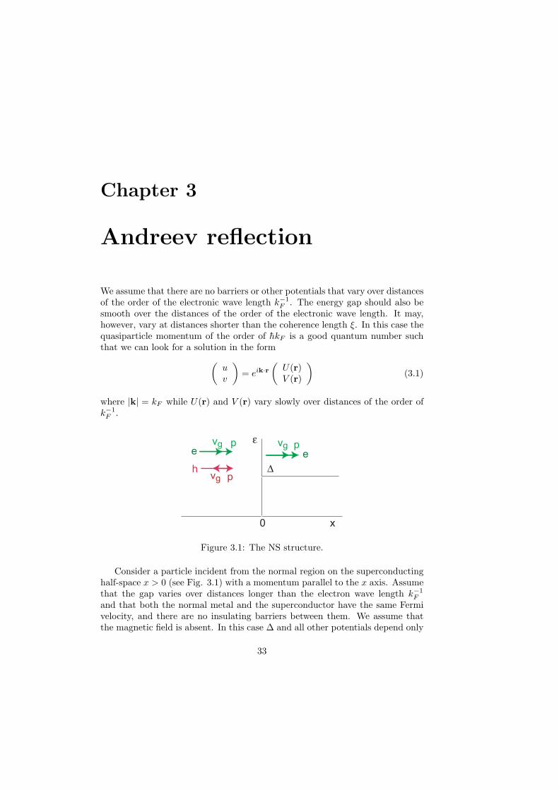
Andreev reflection
We assume that there are no barriers or other potentials that vary over distancesof the order of the electronic wave length k−1
F . The energy gap should also besmooth over the distances of the order of the electronic wave length. It may,however, vary at distances shorter than the coherence length ξ. In this case thequasiparticle momentum of the order of hkF is a good quantum number suchthat we can look for a solution in the form(
uv
)= eik·r
(U(r)V (r)
)(3.1)
where |k| = kF while U(r) and V (r) vary slowly over distances of the order ofk−1
F .
e
h
e
x0
ε
Δvg p
vg p vg p
Figure 3.1: The NS structure.
Consider a particle incident from the normal region on the superconductinghalf-space x > 0 (see Fig. 3.1) with a momentum parallel to the x axis. Assumethat the gap varies over distances longer than the electron wave length k−1
F
and that both the normal metal and the superconductor have the same Fermivelocity, and there are no insulating barriers between them. We assume thatthe magnetic field is absent. In this case Δ and all other potentials depend only
33

34 CHAPTER 3. ANDREEV REFLECTION
pF
pF
-pF
-pF
ε ε
N
0
S
0
iac
Figure 3.2: The Andreev reflection. If the incident state (i) has an energyabove the gap, a transmitted state (c) exists in the superconductor. A particleis partially transmitted and partially reflected back as a hole (a). If the energyis below the gap, there are no states in superconductor, and the particle is fullyreflected back as a hole (a).
on one coordinate x and the BdG equations take the form
− h2
2m
(∂2
∂x2+
∂2
∂y2+
∂2
∂z2
)u− h2k2
F
2mu+ Δ(x)v = εu (3.2)
h2
2m
(∂2
∂x2+
∂2
∂y2+
∂2
∂z2
)v +
h2k2F
2mv + Δ∗(x)u = εv (3.3)
Consider first the case of high energies ε > |Δ|. The particle will penetrateinto the superconductor and partially will be reflected back into the normalmetal. However, since the gap varies slowly, the reflection process where themomentum is changed such that k → −k is prohibited.
In the normal region (on the left) the order parameter decreases to zero atdistances shorter than ξ, so that one can consider Δ = 0 for x < 0. The wavefunctions are(
uv
)L
= ei(kx+ε/hvx)x+ikyy+ikzz
(10
)+ aei(kx−ε/hvx)x+ikyy+ikzz
(01
)(3.4)
Herevx = hkx/m
The wave function thus contains an incident particle [state (i) in Fig. 3.2] and areflected hole [state (a)]. We choose the coefficient unity in front of the incidentwave to ensure the unit density of particles in the incident wave.
The wave function on the right (in the S region) has the form(uv
)R
= cei(kx+λS)x+ikyy+ikzz
(U0
V0
)(3.5)
Eqs. (3.2), (3.3) giveλS =
√ε2 − |Δ|2/hvx (3.6)

35
It describes a transmitted particle. The coherence factors U0 and V0 are deter-mined by Eq. (2.25):
U0 =1√2
[1 +
√ε2 − |Δ|2ε
]1/2
, V0 =1√2
[1 −
√ε2 − |Δ|2ε
]1/2
They satisfy
U20 − V 2
0 =
√ε2 − |Δ|2ε
, U0V0 =|Δ|2ε
The boundary conditions require continuity of the slow functions at theinterface whence
a = V0/U0 , c = 1/U0 (3.7)
The coefficient a describes a process when a particle is reflected as a hole froma spatially non-uniform gap; this process is called the Andreev reflection [9].
For the sub-gap energy ε < |Δ|, there are no states below the gap in the Sregion, thus the wave should decay for x > 0. The wave function on the right is(
uv
)R
= ce(ikx−λS)x+ikyy+ikzz
(U0
V0
)(3.8)
whereλS =
√|Δ|2 − ε2/hvx (3.9)
and
U0 =1√2
(1 + i
√|Δ|2 − ε2
ε
), V0 =
1√2
(1 − i
√|Δ|2 − ε2
ε
)
The coefficients area = V0/U0 , c = 1/U0
However, now|a|2 = 1 (3.10)
The Andreev reflection is complete since there are no transmitted particles.The Andreev reflection has an interesting and surprising property. The
magnitude squared of the particle momentum in Eq. (3.4) is
p2 = p2x +p2
y +p2z = h2[(kx± ε/hvx)2 +k2
y +k2z ] = h2
[k2
F ± 2kxε
hvx
]= h2k2
F ±2mε
The total momentum of the incident particle is thus p = hkF + ε/vF such thatp > pF . Its energy corresponds to the rising (right) part of the spectrum branch[point (i)] in Fig. 3.2,
ε(p) = vF (p− pF )
The reflected hole has the momentum p = pF − ε/vF such that p < pF . Itsenergy thus corresponds to the decreasing (left) part of the spectrum branch[point (a)] in Fig. 3.2,
ε(p) = vF (pF − p)

36 CHAPTER 3. ANDREEV REFLECTION
annihilated hole
penetrating particle incident particle
reflected hole
p
pp
p
vgCooper
pair
N S
-|e|
+|e|
-2|e|
vg
-2|e|
Figure 3.3: Illustration of the nature of Andreev reflection for ε < |Δ at an idealSN interface: An incident electron forms a Cooper pair in the superconductortogether with an annihilated hole. This hole is expelled into the normal metaland moves back as a reflected object.
One can calculate the components of the group velocity
vg x =∂ε
∂px= ±px
m≈ ±vx , vg y =
∂ε
∂py= ±py
m≈ ±vy
We see that particle and hole have opposite signs of the group velocity but withalmost the same magnitude. Therefore, Andreev reflected hole moves along thesame trajectory as the incident particle but in the opposite direction!
q+
q−
h
gv
gve
θ+θ−
x
y
SN
Figure 3.4: The trajectories of an incident particle and the Andreev reflectedhole.
In fact, directions of the incident and reflected trajectories are slightly dif-ferent. Indeed, the change in the momentum during the Andreev reflectionis
Δpx = (hkx − ε/vx) − (hkx + ε/vx) = −2ε/vx
37
This change is much smaller than the momentum itself. This is because theenergy of interaction ∼ Δ is much smaller than EF . At the same time, themomentum projections py and pz are conserved. As a result, the trajectory ofthe reflected hole deviates, but only slightly, from the trajectory of the incidentparticle (see Fig. 3.4).

38 CHAPTER 3. ANDREEV REFLECTION

Chapter 4
Weak links
4.1 Josephson effect
A supercurrent can flow through a junction of two superconductors separatedby narrow constriction, by a normal region or by a high-resistance insulatingbarrier, or by combinations of these. This is the Josephson effect (B. Joseph-son, 1962). The current is a function of the phase difference between the twosuperconductors. These junctions are called weak links. There may be variousdependencies of the current on the phase difference. The form of this dependenceand the maximum supercurrent depend on the conductance of the junction: Thesmaller is the conductance the closer is the dependence to a simple sinusoidalshape.
The presence of a supercurrent is a manifestation of the fundamental prop-erty of the phase coherence that exists between two superconductors separatedby a weak link.
4.1.1 D.C and A.C. Josephson effects
The general features of the Josephson effect can be understood using a verygeneral example of transitions between two superconductors. Assume that twosuperconducting pieces are separated by a thin insulating layer. Electrons cantunnel through this barrier. Assume also that a voltage V is applied betweenthe two superconductors.
The wave function of superconducting electrons is a sum
Ψ =∑α
Cα(t)ψα
of the states ψ1 and ψ2 in superconductor 1 or superconductor 2, respectively.Each wave function ψ1 and ψ2 of an uncoupled superconductor, taken separately,obeys the Schrodinger equation
ih∂ψα
∂t= Eαψα
39

40 CHAPTER 4. WEAK LINKS
χ
χ
2
1
eV
Figure 4.1: The Josephson junction of two superconductors separated by aninsulating barrier.
Here Eα (α = 1, 2) are the energies of the states in uncoupled superconductors1 and 2.
When these superconductors are coupled, the wave function Ψ satisfies theSchrodinger equation
ih∂Ψ∂t
= HΨ
where H is the total Hamiltonian. This equation determines the variations ofthe coefficients. If the wave functions ψα are normalized such that∫
ψ∗βψα dV = δαβ
the coefficients obey
ih∂Cβ
∂t=∑α
[Hβα − Eαδβα]Cα(t) .
HereHβα =
∫ψ∗
βHψα dV
are the matrix elements. The diagonal elements
H11 = E1 + e∗ϕ1 = E1 + e∗V/2 , H22 = E2 + e∗ϕ2 = E2 − e∗V/2
correspond to the energies of the state 1 and 2, respectively. The charge of theCooper pair is e∗ = 2e. The off-diagonal matrix elements describe transitionsbetween the states 1 and 2
H12 = H21 = −K .
The equation becomes
ih∂C1
∂t= eV C1(t) −KC2(t) , (4.1)
ih∂C2
∂t= −KC1(t) − eV C2(t) . (4.2)
4.1. JOSEPHSON EFFECT 41
The coefficients are normalized such that |C1|2 = N1, |C2|2 = N2 where N1,2
are the number of superconducting electrons in the respective electrodes. Weput
C1 =√N1e
iχ1 , C2 =√N2e
iχ2 .
Inserting this into Eqs. (4.1), (4.2) we obtain, separating the real and imaginaryparts
hdN1
dt= −2K
√N1N2 sin(χ2 − χ1)
hdN2
dt= 2K
√N1N2 sin(χ2 − χ1)
and
hN2dχ2
dt= eV N2 +K
√N1N2 cos(χ2 − χ1)
hN1dχ1
dt= −eV N1 +K
√N1N2 cos(χ2 − χ1)
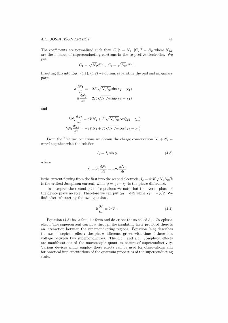
From the first two equations we obtain the charge conservation N1 +N2 =const together with the relation
Is = Ic sinφ (4.3)
where
Is = 2edN2
dt= −2e
dN1
dt
is the current flowing from the first into the second electrode, Ic = 4eK√N1N2/h
is the critical Josephson current, while φ = χ2 − χ1 is the phase difference.To interpret the second pair of equations we note that the overall phase of
the device plays no role. Therefore we can put χ2 = φ/2 while χ1 = −φ/2. Wefind after subtracting the two equations
h∂φ
∂t= 2eV . (4.4)
Equation (4.3) has a familiar form and describes the so called d.c. Josephsoneffect: The supercurrent can flow through the insulating layer provided there isan interaction between the superconducting regions. Equation (4.4) describesthe a.c. Josephson effect: the phase difference grows with time if there is avoltage between two superconductors. The d.c. and a.c. Josephson effectsare manifestations of the macroscopic quantum nature of superconductivity.Various devices which employ these effects can be used for observations andfor practical implementations of the quantum properties of the superconductingstate.

42 CHAPTER 4. WEAK LINKS
1
2
3
4Φ
Ib
I
Ia
Figure 4.2: A SQUID of two Josephson junctions connected in parallel.
4.1.2 Superconducting Quantum Interference Devices
Equation (4.3) form a basis of SQUIDs. Consider a divice consisting of twoJosephson junctions in parallel connected by bulk superconductors, Fig. 4.2.Let us integrate vs defined by Eq. (1.8) along the contour that goes clockwiseall the way inside the superconductors (dashed line in Fig. 4.2). We have
χ3 − χ1 + χ2 − χ4 −2ehc
(∫ 3
1
A · dl +∫ 2
4
A · dl)
= 0
since vs = 0 in the bulk. Neglecting the small sections of the contour betweenthe points 1 and 2 and between 3 and 4, we find
φa − φb =2ehc
∮A · dl =
2πΦΦ0
(4.5)
where φa = χ2 − χ1 and φb = χ4 − χ3.The total current through the device is
I = Ic sinφa + Ic sinφb = 2Ic cos(πΦΦ0
)sin(φa − πΦ
Φ0
).
The maximum current thus depends on the magnetic flux through the loop
Imax = 2Ic cos(πΦΦ0
). (4.6)
Monitoring the current through the SQUID one can measure the magnetic flux.
4.2 Dynamics of Josephson junctions
4.2.1 Resistively shunted Josephson junction
Here we consider the a.c. Josephson effects in systems which carry both Joseph-son and normal currents in presence of a voltage. As we know, the normal cur-rent has a complicated dependence on the applied voltage which is determined

4.2. DYNAMICS OF JOSEPHSON JUNCTIONS 43
R JV
I
Figure 4.3: The resistively shunted Josephson junction.
by particular properties of the junction. In this Section, we consider a simplemodel that treats the normal current as being produced by usual Ohmic resis-tance subject to a voltage V . This current should be added to the supercurrent.Therefore, the total current has the form
I =V
R+ Ic sinφ (4.7)
where the phase difference is φ = χ2 −χ1. Since the Josephson current throughthe junction is small, the current density in the bulk electrodes is also small.Thus, the phases χ1 and χ2 do not vary in the bulk, χ1,2 = const. The differenceof the phases at the both sides from the hole obeys the Josephson relation
h∂φ
∂t= 2eV (4.8)
This equation describes the so called resistively shunted Josephson junction(RSJ) model (see Fig. 4.3).
The full equation for the current is
I =h
2eR∂φ
∂t+ Ic sinφ (4.9)
If I < Ic, the phase is stationary:
φ = arcsin(I/Ic)
and voltage is zero. The phase difference reaches π/2 for I = Ic.If I > Ic, the phase starts to grow with time, and a voltage appears. Let t0
be the time needed for the phase to grow from π/2 to π/2 + 2π. The averagevoltage is then
(2e/h)V = 2π/t0 ≡ ωJ (4.10)
The time t0 is found from Eq. (4.9):
t0 =h
2eR
∫ π/2+2π
π/2
dφ
I − Ic sinφ=
h
2eR
(∫ π/2
−π/2
dφ
I − Ic sinφ+∫ π/2
−π/2
dφ
I + Ic sinφ
)
=Ih
eR
∫ π/2
−π/2
dφ
I2 − I2c sin2 φ
=h
2eR2π√I2 − I2
c

44 CHAPTER 4. WEAK LINKS
II
V
c
Figure 4.4: The current–voltage curve for resistively shunted Josephson junc-tion.
The average voltage is
(2e/h)V = 2π/t0 =2eRh
√I2 − I2
c
The current–voltage curve takes the form
V = R√I2 − I2
c (4.11)
It is shown in Fig. 4.4.
4.2.2 The role of capacitance
The Josephson junction has also a finite capacitance. Let us discuss its effecton the dynamic properties of the junction.
The current through the capacitor (see Fig. 4.5) is
I = C∂V
∂t
The total current becomes
I =hC
2e∂2φ
∂t2+
h
2eR∂φ
∂t+ Ic sinφ (4.12)
Let us discuss this equation. Consider first the work
δA =∫ δt
0
IV dt =h
2eIδφ
produced by an external current source. We find
δA =∫ δt
0
∂
∂t
[h2C
8e2
(∂φ
∂t
)2
− hIc2e
cosφ
]dt+
h2
4e2R
∫ δt
0
(∂φ
∂t
)2
dt
This equation has the form of a balance of energy
δ [Ecapacitor + Ejunction] = δA− h2
4e2R
∫ δt
0
(∂φ
∂t
)2
dt
4.2. DYNAMICS OF JOSEPHSON JUNCTIONS 45
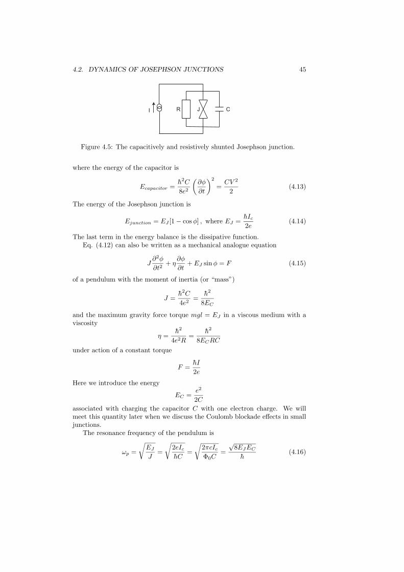
R J CI
Figure 4.5: The capacitively and resistively shunted Josephson junction.
where the energy of the capacitor is
Ecapacitor =h2C
8e2
(∂φ
∂t
)2
=CV 2
2(4.13)
The energy of the Josephson junction is
Ejunction = EJ [1 − cosφ] , where EJ =hIc2e
(4.14)
The last term in the energy balance is the dissipative function.Eq. (4.12) can also be written as a mechanical analogue equation
J∂2φ
∂t2+ η
∂φ
∂t+ EJ sinφ = F (4.15)
of a pendulum with the moment of inertia (or “mass”)
J =h2C
4e2=
h2
8EC
and the maximum gravity force torque mgl = EJ in a viscous medium with aviscosity
η =h2
4e2R=
h2
8ECRC
under action of a constant torque
F =hI
2e
Here we introduce the energy
EC =e2
2Cassociated with charging the capacitor C with one electron charge. We willmeet this quantity later when we discuss the Coulomb blockade effects in smalljunctions.
The resonance frequency of the pendulum is
ωp =
√EJ
J=
√2eIchC
=√
2πcIcΦ0C
=√
8EJEC
h(4.16)
46 CHAPTER 4. WEAK LINKS
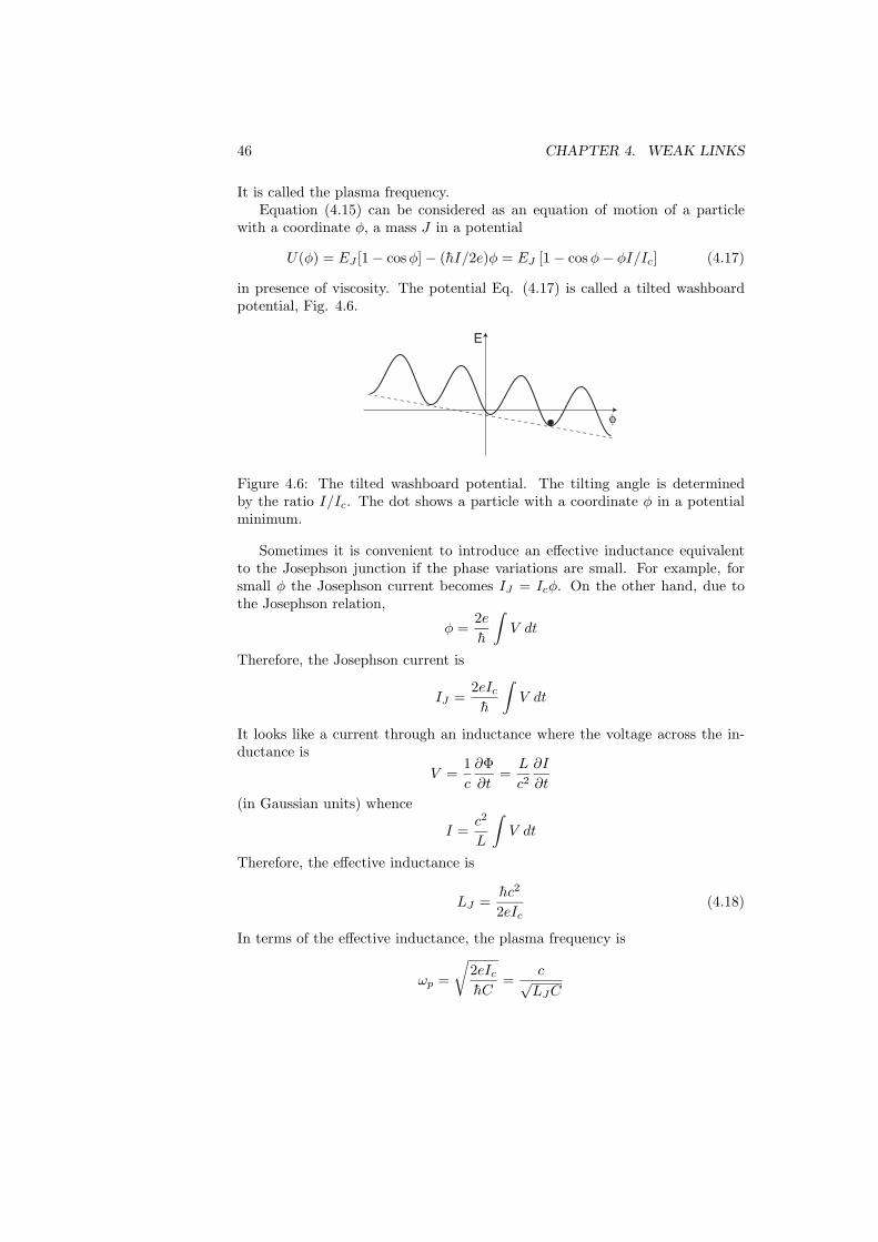
It is called the plasma frequency.Equation (4.15) can be considered as an equation of motion of a particle
with a coordinate φ, a mass J in a potential
U(φ) = EJ [1 − cosφ] − (hI/2e)φ = EJ [1 − cosφ− φI/Ic] (4.17)
in presence of viscosity. The potential Eq. (4.17) is called a tilted washboardpotential, Fig. 4.6.
E
φ
Figure 4.6: The tilted washboard potential. The tilting angle is determinedby the ratio I/Ic. The dot shows a particle with a coordinate φ in a potentialminimum.
Sometimes it is convenient to introduce an effective inductance equivalentto the Josephson junction if the phase variations are small. For example, forsmall φ the Josephson current becomes IJ = Icφ. On the other hand, due tothe Josephson relation,
φ =2eh
∫V dt
Therefore, the Josephson current is
IJ =2eIch
∫V dt
It looks like a current through an inductance where the voltage across the in-ductance is
V =1c
∂Φ∂t
=L
c2∂I
∂t
(in Gaussian units) whence
I =c2
L
∫V dt
Therefore, the effective inductance is
LJ =hc2
2eIc(4.18)
In terms of the effective inductance, the plasma frequency is
ωp =
√2eIchC
=c√LJC
4.2. DYNAMICS OF JOSEPHSON JUNCTIONS 47
which coincides with the resonance frequency of an LC circuit.Equation (4.12) can be written also as
ω−2p
∂2φ
∂t2+Q−1ω−1
p
∂φ
∂t+ sinφ =
I
Ic(4.19)
where we introduce the quality factor
Q = ωpRC =
√2eIcR2C
h(4.20)
that characterizes the relative dissipation in the system. This parameter is largewhen resistance is large so that the normal current and dissipation are small.
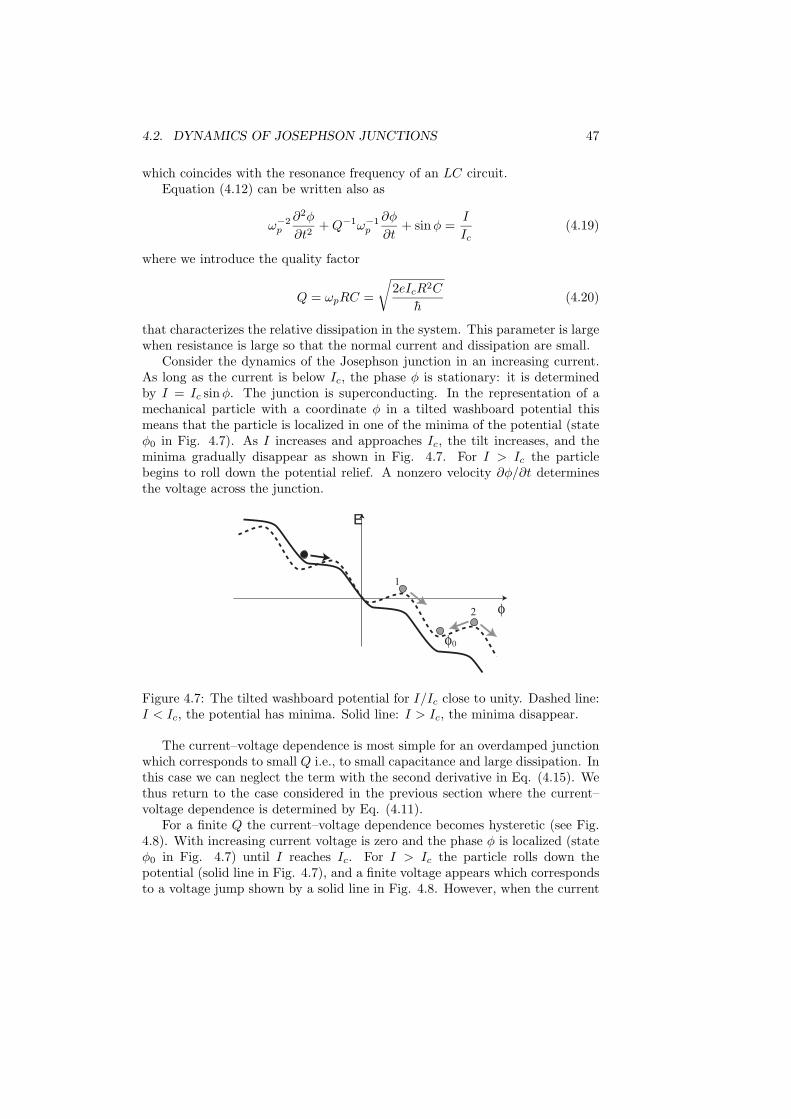
Consider the dynamics of the Josephson junction in an increasing current.As long as the current is below Ic, the phase φ is stationary: it is determinedby I = Ic sinφ. The junction is superconducting. In the representation of amechanical particle with a coordinate φ in a tilted washboard potential thismeans that the particle is localized in one of the minima of the potential (stateφ0 in Fig. 4.7). As I increases and approaches Ic, the tilt increases, and theminima gradually disappear as shown in Fig. 4.7. For I > Ic the particlebegins to roll down the potential relief. A nonzero velocity ∂φ/∂t determinesthe voltage across the junction.
E
φ
1
2
φ0
Figure 4.7: The tilted washboard potential for I/Ic close to unity. Dashed line:I < Ic, the potential has minima. Solid line: I > Ic, the minima disappear.
The current–voltage dependence is most simple for an overdamped junctionwhich corresponds to small Q i.e., to small capacitance and large dissipation. Inthis case we can neglect the term with the second derivative in Eq. (4.15). Wethus return to the case considered in the previous section where the current–voltage dependence is determined by Eq. (4.11).
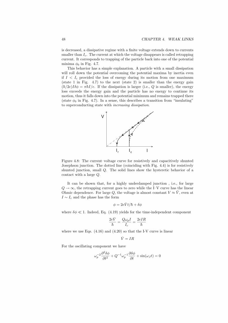
For a finite Q the current–voltage dependence becomes hysteretic (see Fig.4.8). With increasing current voltage is zero and the phase φ is localized (stateφ0 in Fig. 4.7) until I reaches Ic. For I > Ic the particle rolls down thepotential (solid line in Fig. 4.7), and a finite voltage appears which correspondsto a voltage jump shown by a solid line in Fig. 4.8. However, when the current
48 CHAPTER 4. WEAK LINKS
is decreased, a dissipative regime with a finite voltage extends down to currentssmaller than Ic. The current at which the voltage disappears is called retrappingcurrent. It corresponds to trapping of the particle back into one of the potentialminima φ0 in Fig. 4.7.
This behavior has a simple explanation. A particle with a small dissipationwill roll down the potential overcoming the potential maxima by inertia evenif I < Ic provided the loss of energy during its motion from one maximum(state 1 in Fig. 4.7) to the next (state 2) is smaller than the energy gain(h/2e)Iδφ = πhI/e. If the dissipation is larger (i.e., Q is smaller), the energyloss exceeds the energy gain and the particle has no energy to continue itsmotion, thus it falls down into the potential minimum and remains trapped there(state φ0 in Fig. 4.7). In a sense, this describes a transition from “insulating”to superconducting state with increasing dissipation.
II
V
cIr
Figure 4.8: The current–voltage curve for resistively and capacitively shuntedJosephson junction. The dotted line (coinciding with Fig. 4.4) is for resistivelyshunted junction, small Q. The solid lines show the hysteretic behavior of acontact with a large Q.
It can be shown that, for a highly underdamped junction , i.e., for largeQ→ ∞, the retrapping current goes to zero while the I–V curve has the linearOhmic dependence. For large Q, the voltage is almost constant V ≈ V , even atI ∼ Ic and the phase has the form
φ = 2eV t/h+ δφ
where δφ� 1. Indeed, Eq. (4.19) yields for the time-independent component
2eVh
=QωpI
Ic=
2eIRh
where we use Eqs. (4.16) and (4.20) so that the I-V curve is linear
V = IR
For the oscillating component we have
ω−2p
∂2δφ
∂t2+Q−1ω−1
p
∂δφ
∂t+ sin(ωJ t) = 0
4.2. DYNAMICS OF JOSEPHSON JUNCTIONS 49
where we put
ωJ =2eVh
For a large Q we neglect the first derivative and find
δφ =ω2
p
ω2J
sin(ωJ t)
The variation δφ is small if ωp/ωJ � 1. This condition reads
ω2p
ωpωJ=
IcIωpRC
=IcIQ
� 1
Therefore it should be Ic/IQ� 1. If the current does not satisfy this condition,δφ becomes large, and the finite voltage regime breaks down. Therefore, theretrapping current is
Ir ∼ Ic/Q (4.21)
It goes to zero as Q→ ∞.
4.2.3 Thermal fluctuations
Consider first overdamped junction. A particle with a coordinate φ is mostlysitting in one of the minima of the washboard potential in Fig. 4.6. It cango into the state in a neighboring minimum if it receives the energy enough toovercome the barrier. This energy can come from the heat bath, for example,from phonons. The probability of such a process is proportional to exp(−U/T )where U is the height of the barrier as seen from the current state of the particle.The probability P+ to jump over the barrier from the state φ0 to the state φ0+2πand the probability P− to jump over the barrier from the state φ0 + 2π back tothe state φ0 are
P± = ωa exp[−U0 ∓ (πhI/2e)
T
]where ωa is a constant attempt frequency, and U0 is the average barrier height.Therefore, the probability that the particle will go from the state φ0 to the stateφ0 + 2π is
P = P+ − P− = 2ωa exp[−U0
T
]sinh
(πhI
2eT
)This will produce a finite voltage
V =(h
2e
)2πP =
2πhωa
eexp
[−U0
T
]sinh
(πhI
2eT
)
For low currents, I � Ic, the barrier height is independent of the currentU0 = 2EJ . For I → 0 we find
V =π2h2ωaI
e2Texp
(−2EJ
T
)
50 CHAPTER 4. WEAK LINKS
II
V
c
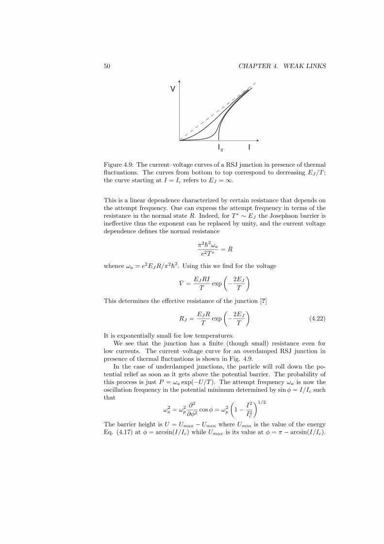
Figure 4.9: The current–voltage curves of a RSJ junction in presence of thermalfluctuations. The curves from bottom to top correspond to decreasing EJ/T ;the curve starting at I = Ic refers to EJ = ∞.
This is a linear dependence characterized by certain resistance that depends onthe attempt frequency. One can express the attempt frequency in terms of theresistance in the normal state R. Indeed, for T ∗ ∼ EJ the Josephson barrier isineffective thus the exponent can be replaced by unity, and the current voltagedependence defines the normal resistance
π2h2ωa
e2T ∗ = R
whence ωa = e2EJR/π2h2. Using this we find for the voltage
V =EJRI
Texp
(−2EJ
T
)
This determines the effective resistance of the junction [?]
RJ =EJR
Texp
(−2EJ
T
)(4.22)
It is exponentially small for low temperatures.We see that the junction has a finite (though small) resistance even for
low currents. The current–voltage curve for an overdamped RSJ junction inpresence of thermal fluctuations is shown in Fig. 4.9.
In the case of underdamped junctions, the particle will roll down the po-tential relief as soon as it gets above the potential barrier. The probability ofthis process is just P = ωa exp(−U/T ). The attempt frequency ωa is now theoscillation frequency in the potential minimum determined by sinφ = I/Ic suchthat
ω2a = ω2
p
∂2
∂φ2cosφ = ω2
p
(1 − I2
I2c
)1/2
The barrier height is U = Umax − Umin where Umin is the value of the energyEq. (4.17) at φ = arcsin(I/Ic) while Umax is its value at φ = π − arcsin(I/Ic).
4.2. DYNAMICS OF JOSEPHSON JUNCTIONS 51
Therefore
U = 2EJ
[cos arcsin
I
Ic− I
Icarccos
I
Ic
]
= 2EJ
√1 − I2
I2c
− 2IEJ
Icarccos
(I
Ic
)(4.23)
The probability is more important for large currents I → Ic when the barrier issmall,
U ≈ 4√
23EJ (1 − I/Ic)
3/2 (4.24)
As the current increases from zero to Ic the probability P = ωa exp(−U/T )of an escape from the potential minimum increases from exponentially smallup to P ∼ ωp ∼ 1010 sec−1. The voltage generated by escape processes isV ∼ (πh/e)P .
The rising part of the I–V curve in Fig. 4.9 for an overdamped junction nearIc is also determined by an exponential dependence V = (πh/e)P+ where theprobability P+ contains the barrier from Eq. (4.24). Indeed, the probabilityof the reverse process P− is now strongly suppressed by a considerably higherbarrier seen from the next potential minimum.
4.2.4 Shapiro steps
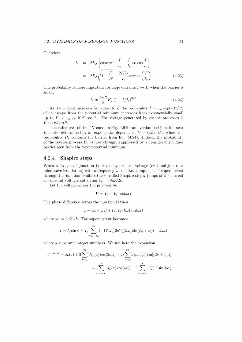
When a Josephson junction is driven by an a.c. voltage (or is subject to amicrowave irradiation) with a frequency ω, the d.c. component of supercurrentthrough the junction exhibits the so called Shapiro steps: jumps of the currentat constant voltages satisfying Vn = nhω/2e.
Let the voltage across the junction be
V = V0 + V1 cos(ωt)
The phase difference across the junction is then
φ = φ0 + ωJ t+ (2eV1/hω) sin(ωt)
where ωJ = 2eV0/h. The supercurrent becomes
I = Ic sinφ = Ic
∞∑k=−∞
(−1)kJk(2eV1/hω) sin(φ0 + ωJ t− kωt)
where k runs over integer numbers. We use here the expansion
eiz sin α = J0(z) + 2∞∑
k=1
J2k(z) cos(2kα) + 2i∞∑
k=0
J2k+1(z) sin[(2k + 1)α]
=∞∑
k=−∞Jk(z) cos(kα) + i
∞∑k=−∞
Jk(z) sin(kα)
52 CHAPTER 4. WEAK LINKS
I
V
ΔI1
hω/2e
2hω/2e
3hω/2e
Figure 4.10: The current–voltage curves of a RSJ junction irradiated by a mi-crowave with frequency ω.
with z = 2eV1/hω and α = ωt. We note that due the parity Jk(z) = (−1)kJ−k(z)of the Bessel functions, the components with odd k drop out from the first sumin the second line, while the components with even k drop out from the secondsum. Using this we arrive at the above expression for the current.
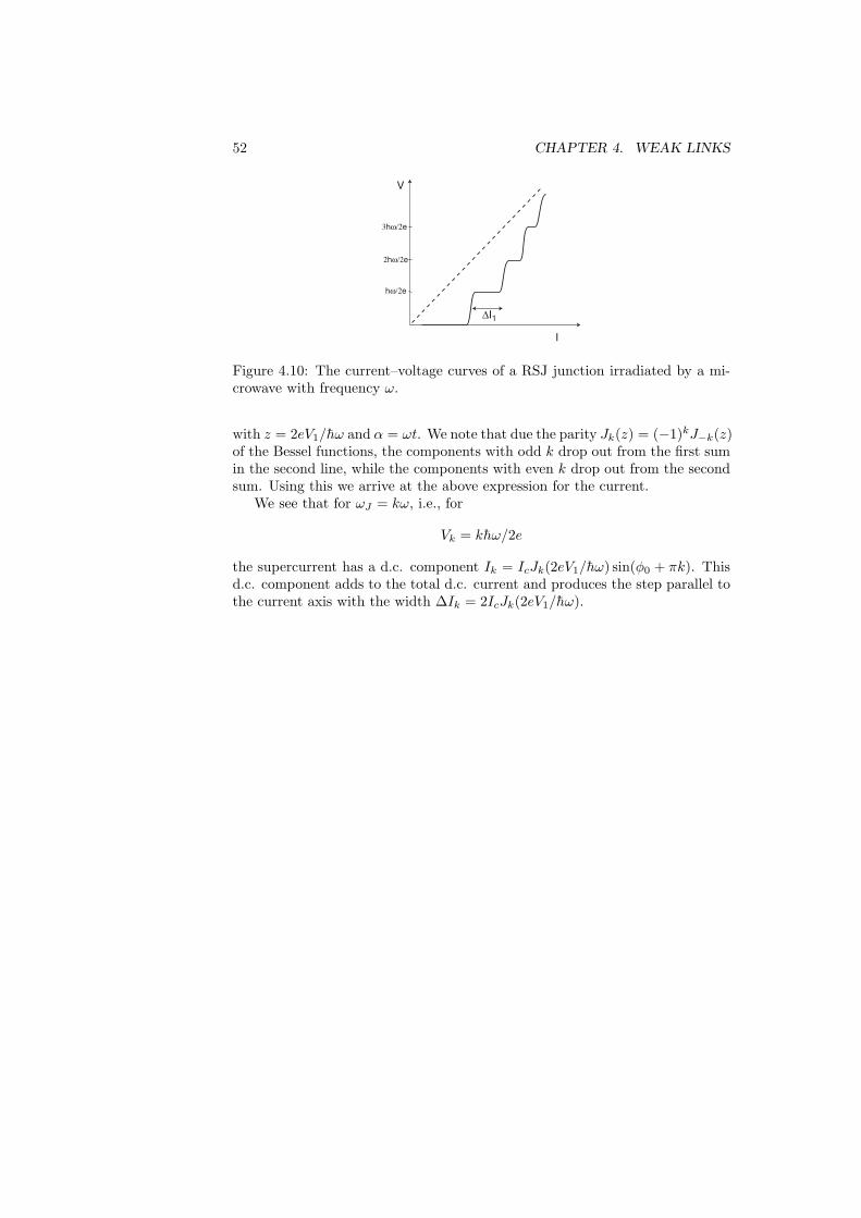
We see that for ωJ = kω, i.e., for
Vk = khω/2e
the supercurrent has a d.c. component Ik = IcJk(2eV1/hω) sin(φ0 + πk). Thisd.c. component adds to the total d.c. current and produces the step parallel tothe current axis with the width ΔIk = 2IcJk(2eV1/hω).

Chapter 5
Coulomb blockade innormal double junctions
5.1 Orthodox description of the Coulomb block-ade
See [12]. For more detailed description including the effects of environment see,for example, review [13], [15].
C1, R1 C2, R2
V1 V2Vg
Cg
Island
Figure 5.1: The equivalent circuit of a SET. The island is coupled to the voltagesource via two contacts with resistances R1, R2 and capacitances C1, C2, andto the gate through the capacitor Cg. The bias voltage is V = V1 − V2.
Consider the device called the single electron transistor (SET) with theequivalent circuit shown in Fig. 5.1. For simplicity we assume a symmetricsituation C1 = C2, R1 = R2 ≡ RT such that V1 = V/2, V2 = −V/2, and thatthe capacitance of the gate Cg is small. Let the charge on the island providedby the gate voltage be Q0 = VgCg.
For zero bias voltage V = 0, the electrostatic energy of the island havinga charge Q consisting of the continuous offset charge Q0 provided by the gateelectrode and a discrete charge of k electrons that have tunneled into the island,
53
54CHAPTER 5. COULOMB BLOCKADE IN NORMAL DOUBLE JUNCTIONS
e/2 3e/2-3e/2 0 Q0
E
e-e -e/2 2e-2e
k=0 k=-1k=1
Figure 5.2:
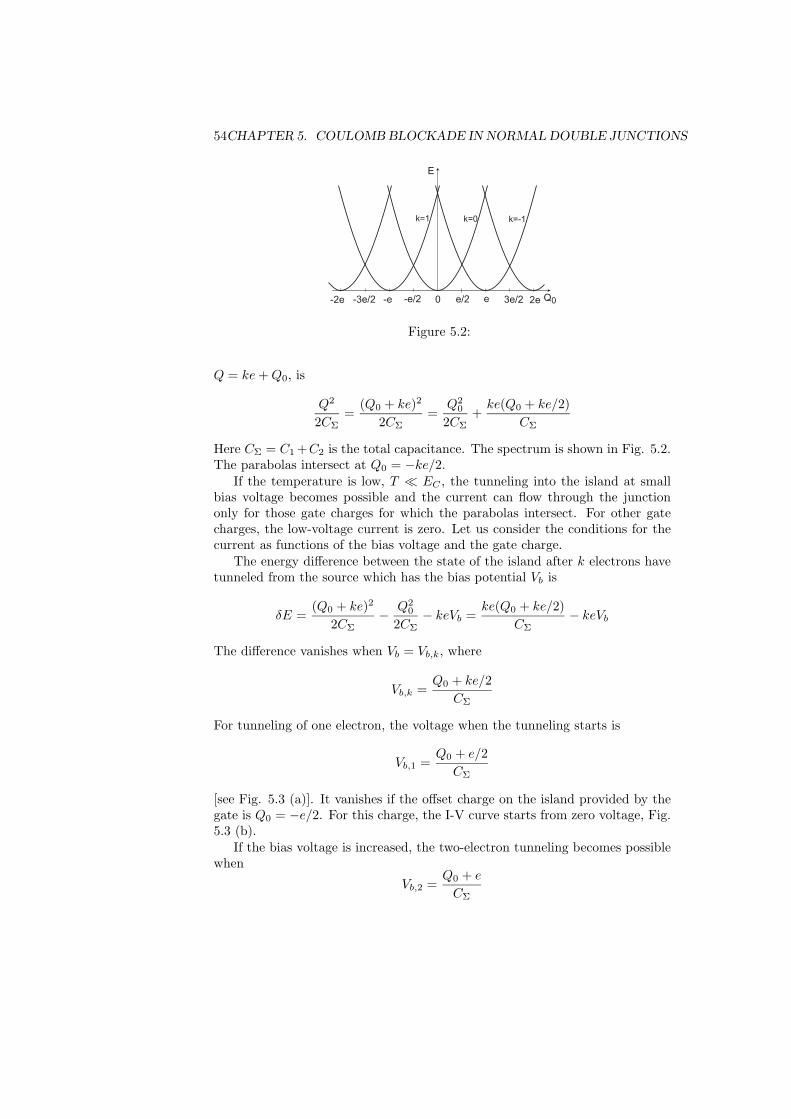
Q = ke+Q0, is
Q2
2CΣ=
(Q0 + ke)2
2CΣ=
Q20
2CΣ+ke(Q0 + ke/2)
CΣ
Here CΣ = C1 +C2 is the total capacitance. The spectrum is shown in Fig. 5.2.The parabolas intersect at Q0 = −ke/2.
If the temperature is low, T � EC , the tunneling into the island at smallbias voltage becomes possible and the current can flow through the junctiononly for those gate charges for which the parabolas intersect. For other gatecharges, the low-voltage current is zero. Let us consider the conditions for thecurrent as functions of the bias voltage and the gate charge.
The energy difference between the state of the island after k electrons havetunneled from the source which has the bias potential Vb is
δE =(Q0 + ke)2
2CΣ− Q2
0
2CΣ− keVb =
ke(Q0 + ke/2)CΣ
− keVb
The difference vanishes when Vb = Vb,k, where
Vb,k =Q0 + ke/2
CΣ
For tunneling of one electron, the voltage when the tunneling starts is
Vb,1 =Q0 + e/2CΣ
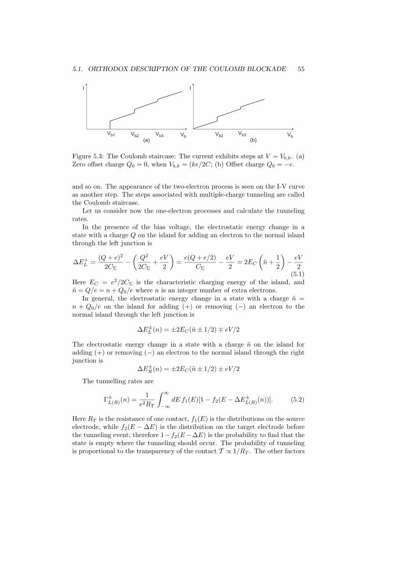
[see Fig. 5.3 (a)]. It vanishes if the offset charge on the island provided by thegate is Q0 = −e/2. For this charge, the I-V curve starts from zero voltage, Fig.5.3 (b).
If the bias voltage is increased, the two-electron tunneling becomes possiblewhen
Vb,2 =Q0 + e
CΣ
5.1. ORTHODOX DESCRIPTION OF THE COULOMB BLOCKADE 55
Vb1 Vb2 Vb3 Vb
I
(a)Vb2
Vb3 Vb
I
(b)
Figure 5.3: The Coulomb staircase: The current exhibits steps at V = Vb,k. (a)Zero offset charge Q0 = 0, when Vb,k = (ke/2C; (b) Offset charge Q0 = −e.
and so on. The appearance of the two-electron process is seen on the I-V curveas another step. The steps associated with multiple-charge tunneling are calledthe Coulomb staircase.
Let us consider now the one-electron processes and calculate the tunnelingrates.
In the presence of the bias voltage, the electrostatic energy change in astate with a charge Q on the island for adding an electron to the normal islandthrough the left junction is
ΔE+L =
(Q+ e)2
2CΣ−(Q2
2CΣ+eV
2
)=e(Q+ e/2)
CΣ− eV
2= 2EC
(n+
12
)− eV
2(5.1)
Here EC = e2/2CΣ is the characteristic charging energy of the island, andn = Q/e = n+Q0/e where n is an integer number of extra electrons.
In general, the electrostatic energy change in a state with a charge n =n + Q0/e on the island for adding (+) or removing (−) an electron to thenormal island through the left junction is
ΔE±L (n) = ±2EC(n± 1/2) ∓ eV/2
The electrostatic energy change in a state with a charge n on the island foradding (+) or removing (−) an electron to the normal island through the rightjunction is
ΔE±R (n) = ±2EC(n± 1/2) ± eV/2
The tunnelling rates are
Γ±L(R)(n) =
1e2RT
∫ ∞
−∞dE f1(E)[1 − f2(E − ΔE±
L(R)(n))]. (5.2)
Here RT is the resistance of one contact, f1(E) is the distributions on the sourceelectrode, while f2(E − ΔE) is the distribution on the target electrode beforethe tunneling event; therefore 1−f2(E−ΔE) is the probability to find that thestate is empty where the tunneling should occur. The probability of tunnelingis proportional to the transparency of the contact T ∝ 1/RT . The other factors
56CHAPTER 5. COULOMB BLOCKADE IN NORMAL DOUBLE JUNCTIONS
in the coefficient in front of the integral in Γ are chosen in such a way as toprovide the correct expression for the resistance of the contact in the Ohmicregime, see Eq. (5.7) below.
For equilibrium distribution fi(E) = (1 + eE/Ti)−1 with T1 = T2,we have
f(E)[1 − f(E − ΔE±(n))] =f(E) − f(E − ΔE±)
1 − exp(ΔE±/T )
One can also prove that∫ ∞
−∞dE [f(E) − f(E + x)] = x
Therefore, Eq. (5.2) yields
Γ±(n) =1
e2RT
ΔE±
exp(ΔE±/T ) − 1(5.3)
The current into the island through the left (right) junction is
IL(R) = e
∞∑n=−∞
σ(n)[Γ+L(R)(n) − Γ−
L(R)(n)] (5.4)
where σ(n) is the probability of having n extra electrons on the island. We have
∞∑n=−∞
nσ(n) = 0 (5.5)
by symmetry, and
∞∑n=−∞
σ(n) = 1 ,∞∑
n=−∞nσ(n) = Q0/e (5.6)
5.1.1 Low temperature limit
For T → 0 the tunneling rates Eq. (5.3) are
Γ±L(R)(n) =
1e2RT
|ΔE±L(R)|Θ(−ΔE±
L(R))
The rates vanish when all ΔE±L(R) are positive. This takes place when
ΔE(+)L > 0 : eV/2 − 2EC(n+ 1/2) < 0 (a)
ΔE(−)L > 0 : eV/2 − 2EC(n− 1/2) > 0 (b)
ΔE(+)R > 0 : eV/2 + 2EC(n+ 1/2) > 0 (c)
ΔE(−)R > 0 : eV/2 + 2EC(n− 1/2) < 0 (d)

5.1. ORTHODOX DESCRIPTION OF THE COULOMB BLOCKADE 57
(a)
(b)
(c)
(d)V
Qe/2-e/2
e/C
-e/C
Figure 5.4: The region of stable charge is shaded. The lines (a)–(d) correspondto equalities in Eqs. (a) to (d).
V
Q0e/2-e/2 3e/2-3e/2
n=0n=1 n=-1
Figure 5.5: The regions of stable charge n = 0,±1, . . . as functions of the gatecharge.
In Fig. 5.4 the diamond-shaped region in the plane (V,Q = en) is shaded whereall the rates are zero. This is the region where the current to and out of theisland is zero, and the charge on the island does not change due to the Coulombblockade. If the offset charge Q0 is in the range −e/2 < Q0 < e/2, the statewith n = 0 is stable.
With change in the gate voltage, the stable charge on the island will vary byinteger number of electrons due to tunneling to or from the respective electrode.The regions of stable states with n = 0,±e, . . . as functions of the gate chargeare shown in Fig. 5.5.
5.1.2 Conductance in the high temperature limit
We have for the left junction
Γ+L(n) − Γ−
L (n) =1
e2RT
[ΔE+
L
exp(ΔE+L /T ) − 1
− ΔE−L
exp(ΔE−L /T ) − 1
]
Up to the first order in EC/kBTe we have
Γ+L(n) − Γ−
L (n) =T
e2RT
[v
(1
1 − ev+
11 − e−v
)
−2nEC
T[f(v) + f(−v)] +
EC
T[f(v) − f(−v)]
]
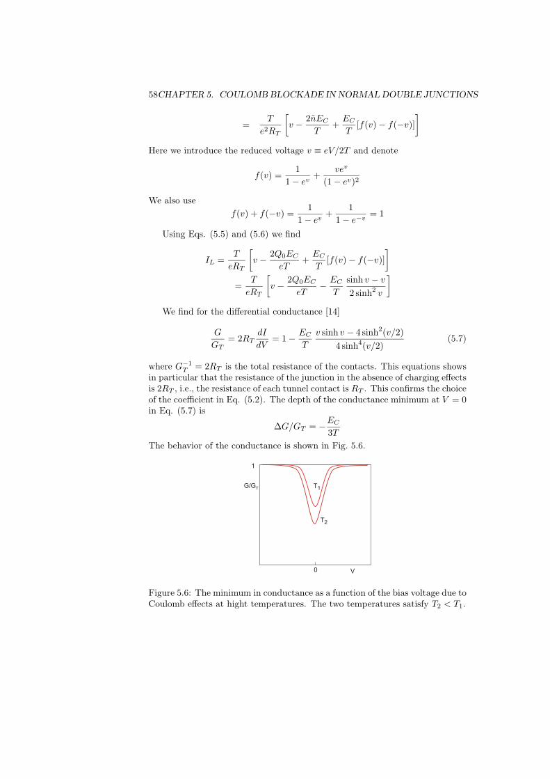
58CHAPTER 5. COULOMB BLOCKADE IN NORMAL DOUBLE JUNCTIONS
=T
e2RT
[v − 2nEC
T+EC
T[f(v) − f(−v)]
]
Here we introduce the reduced voltage v ≡ eV/2T and denote
f(v) =1
1 − ev+
vev
(1 − ev)2
We also usef(v) + f(−v) =
11 − ev
+1
1 − e−v= 1
Using Eqs. (5.5) and (5.6) we find
IL =T
eRT
[v − 2Q0EC
eT+EC
T[f(v) − f(−v)]
]
=T
eRT
[v − 2Q0EC
eT− EC
T
sinh v − v
2 sinh2 v
]
We find for the differential conductance [14]
G
GT= 2RT
dI
dV= 1 − EC
T
v sinh v − 4 sinh2(v/2)4 sinh4(v/2)
(5.7)
where G−1T = 2RT is the total resistance of the contacts. This equations shows
in particular that the resistance of the junction in the absence of charging effectsis 2RT , i.e., the resistance of each tunnel contact is RT . This confirms the choiceof the coefficient in Eq. (5.2). The depth of the conductance minimum at V = 0in Eq. (5.7) is
ΔG/GT = −EC
3TThe behavior of the conductance is shown in Fig. 5.6.
V0
G/GT
1
T1
T2
Figure 5.6: The minimum in conductance as a function of the bias voltage due toCoulomb effects at hight temperatures. The two temperatures satisfy T2 < T1.
Chapter 6
Quantum phenomena inJosephson junctions
6.1 Quantization
6.1.1 Quantum conditions
Quantum effects can be observed in Josephson structures consisting, for exam-ple, of a very small superconducting grain connected to superconducting chargereservoirs through small tunnel junctions having very low capacitance and hightunnel resistance, as shown in Fig. 6.1. The equivalent circuit is shown in Fig.5.1. The necessary constraints can be easily estimated from general arguments.First, the Coulomb charging energy for one electron e2/2C should be larger thantemperature T to avoid thermal smearing of the charge states on the supercon-ducting island. For T ∼ 1 K this gives C < 10−15 F which strongly restrictsthe size of the junction by an area ∼ 10−8 cm2. Second, the tunnel resistanceshould be large enough to avoid averaging out by quantum fluctuations in theparticle number. To be observable, the charging energy e2/2C must exceed thequantum uncertainty in energy h/Δt ∼ h/RC associated with the finite life-time of the charge on the capacitor. Equating e2/2C to h/RC we find thatthe capacitance drops out and the condition becomes R > R0 where R0 is theresistance quantum R0 = h/2e2 ≈ 12 kΩ, the quantity already familiar fromEq. (??).
Another realization may be a small Josephson junction with a capacitanceC and tunnel resistance R satisfying the above conditions, which is connectedthrough small-capacitance, Cext � C, high-resistance contacts such that R0 �Rext � R to the external current source, Fig. 6.2. The detailed description ofquantum phenomena can be found, for example, in review [13].
59
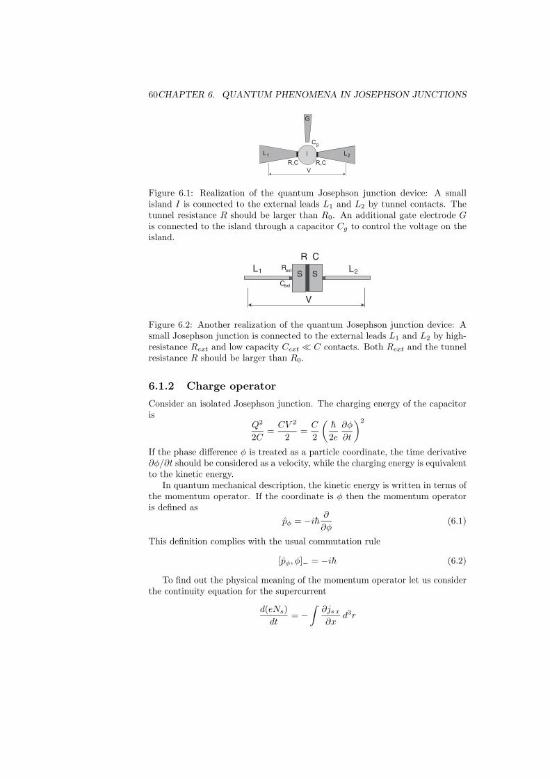
60CHAPTER 6. QUANTUM PHENOMENA IN JOSEPHSON JUNCTIONS
V
R,C R,C
L I
G
1 L2
Cg
Figure 6.1: Realization of the quantum Josephson junction device: A smallisland I is connected to the external leads L1 and L2 by tunnel contacts. Thetunnel resistance R should be larger than R0. An additional gate electrode Gis connected to the island through a capacitor Cg to control the voltage on theisland.
R
R C
S Sext
extC
V
L1 L2
Figure 6.2: Another realization of the quantum Josephson junction device: Asmall Josephson junction is connected to the external leads L1 and L2 by high-resistance Rext and low capacity Cext � C contacts. Both Rext and the tunnelresistance R should be larger than R0.
6.1.2 Charge operator
Consider an isolated Josephson junction. The charging energy of the capacitoris
Q2
2C=CV 2
2=C
2
(h
2e∂φ
∂t
)2
If the phase difference φ is treated as a particle coordinate, the time derivative∂φ/∂t should be considered as a velocity, while the charging energy is equivalentto the kinetic energy.
In quantum mechanical description, the kinetic energy is written in terms ofthe momentum operator. If the coordinate is φ then the momentum operatoris defined as
pφ = −ih ∂
∂φ(6.1)
This definition complies with the usual commutation rule
[pφ, φ]− = −ih (6.2)
To find out the physical meaning of the momentum operator let us considerthe continuity equation for the supercurrent
d(eNs)dt
= −∫∂js x
∂xd3r

6.1. QUANTIZATION 61
The current density j has the form of the charge flow density ensvs which is
e∂Es
∂ps
where ps is the momentum of a superconducting particle and Es is the super-conducting energy density. The momentum of the Cooper pair is 2ps = h∂χ/∂xso that the continuity equation takes the form
d(eNs)dt
= −e∫
∂
∂x
∂Es
∂psd3r = −2e
h
∫∂
∂x
∂Es
∂(φ/x)d3r = −2e
h
∂Es
∂φ
since the phase gradient over the length x is ∂χ/∂x = φ/x where φ is the (given)phase difference. The quantity
Es =∫Es d
3r
is the superconducting energy. Therefore,
h
2dNs
dt= −∂Es
∂φ(6.3)
This equation can be considered as one of the Hamiltonian equations ∂p/∂t =−∂H/∂x. Since φ is the coordinate and E is the energy, the quantity hNs/2 isthe momentum of the particle. However, according to Eq. (6.2) the canonicallyconjugated momentum operator is pφ. Therefore, pφ = hNs/2 and
−i ∂∂φ
=Ns
2= Np (6.4)
is the operator of the number of Cooper pairs Np = Ns/2. The second Hamil-tonian equation has the form
∂x
∂t=∂H∂p
⇒ ∂φ
∂t=
E∂(hNs/2)
or12∂φ
∂t=
∂Es
∂(hNs)=μs
h
where μs is the chemical potential of Cooper pairs. This equation coincides withthe Josephson relation since μs = eV .
Equation (6.4) defines the operator of “superconducting charge” transferredthrough the junction
Q = eNs = 2eNp = −2ie∂
∂φ(6.5)
The commutation relation takes the form
[Q, φ]− = −2ie
Therefore, the quantum uncertainty in phase Δφ and in charge ΔQ are restrictedby the charge of a Cooper pair ΔφΔQ ∼ 2e.
62CHAPTER 6. QUANTUM PHENOMENA IN JOSEPHSON JUNCTIONS
The eigenfunction of a state with the charge Q obeys the equation
QΨQ = QΨQ or − 2ie∂ΨQ
∂φ= QΨQ
It isΨQ(φ) = CeiQφ/2e (6.6)
Assuming a single-valued wave function
ΨQ(φ+ 2π) = ΨQ(φ)
we obtain quantization of charge of a Cooper pair πQ/e = 2πn, i.e.,
Q = 2en
where n is a integer.Note that φ is the phase of the wave function of a Cooper pair of electrons.
The single electron phase would be φ1 = φ/2. If we now require a single-valuedone-electron wave function,
ΨQ(φ1) = CeiQφ1/e
so that Ψ(φ1 + 2π) = Ψ(φ1), we obtain 2πQ/e = 2πn such that the single-electron charge is integer: Q = en.
6.1.3 The Hamiltonian
The charging energy of a capacitor can be written as
Q2
2C= −4e2
2C∂2
∂φ2= −4EC
∂2
∂φ2
where
EC =e2
2Cis the the charging energy for the charge of one electron.
The total energy of the Josephson junction becomes
H = −4EC∂2
∂φ2+ EJ [1 − cosφ] (6.7)
This is the Hamiltonian of the junction in the quantum mechanical description.If the junction is connected to a current source, the charge operator changes
Q = −2ie∂
∂φ+ q(t)
where q(t) is a continuous charge supplied by the current source. The Hamilto-nian becomes
H = 4EC
(−i ∂∂φ
+q(t)2e
)2
+ EJ [1 − cosφ] (6.8)
6.2. MACROSCOPIC QUANTUM TUNNELLING 63
In the classical limit this Hamiltonian is equivalent to the washboard poten-tial. Indeed, the classical analogue of Eq. (6.8) is
E =[Q+ q(t)]2
2C+ EJ [1 − cosφ]
where Q is the charge that is transferred through the junction. Using theJosephson relation V = (h/2e)(dφ/dt) the charging energy can be transformedas
[Q+ q(t)]2
2C=
Q2
2C+
[Q+ q(t)]q(t)C
− q2(t)2C
=Q2
2C+ V q(t) − q2(t)
2C=Q2
2C− hφ
2edq
dt+
d
dt
[hφ
2eq(t)
]− q2(t)
2C
=Q2
2C− hφ
2eI +
dF (t)dt
Here I = dq/dt. The last term dF (t)/dt is a full derivative of certain function.It can be omitted. With Eq. (6.5) for the operator Q, the total Hamiltonianassumes the usual form of a Hamiltonian of a particle in the tilted washboardpotential
H = −4EC∂2
∂φ2+ EJ [1 − cosφ] − hI
2eφ (6.9)
The quantum-mechanical description goes over into the classical picture de-scribed in Chapter 4 when the charge Q in the charge eigen-function Eq. (6.6) islarge as compared to the electron charge and can be considered as a continuousvariable.
6.2 Macroscopic quantum tunnelling
With the account of quantum effects, the behavior of the junction in presenceof a high bias current is different from that considered in the previous chapter.Consider the Hamiltonian Eq. (6.9) for a representative particle in a washboardpotential. The representative particle with the coordinate φ can now escapefrom the potential minimum at φ0 by tunnelling through the potential barrier,see Fig. 6.3, maximum 1. If the maximum 2 in Fig. 6.3 is lower than theminimum φ0, the particle needs one tunnelling through the barrier shown by agray region in the figure.
Tunnelling of the representative particle means a tunnelling of the entiresystem from one macroscopic state that contains many particles to anothermacroscopic state. This process involves a macroscopic number of particlesand thus its probability should be inherently small. However, the Josephsonjunction provides a tool that can help us to observe these macroscopic quantumtunnelling (MQT) events.
The easiest way to solve the Schrodinger equation[−4EC
∂2
∂φ2+ U(φ)
]Ψ(φ) = EΨ(φ)

64CHAPTER 6. QUANTUM PHENOMENA IN JOSEPHSON JUNCTIONS
E
φ1
2φ0
0
Figure 6.3: The tilted washboard potential in the quantum case. A quantumparticle can escape from the potential minimum by tunnelling through the bar-rier (grey region).
with the washboard potential
U(φ) = EJ
[1 − cosφ− I
Icφ
]
is to use the WKB approximation
Ψ = exp(i
∫λ(φ) dφ
)
assuming dλ/dφ� λ2. We find
λ2 =E − UJ(φ)
4EC
The WKB approximation holds if dU/dφ� λ3EC or when EJ � EC .For the energy below the potential maximum we have
λ = iλ =i√UJ(φ) − E
2E1/2C
which ensures the decay of the wave function for positive φ. The transmissionprobability through the barrier is proportional to the square of the transmissionamplitude
exp
(−∫ φ′
φ0
λ dφ
)
where φo and φ′ are the turning points satisfying E = U(φ). The probability oftunnelling becomes
P ∼ ωa exp
(−E−1/2
C
∫ φ′
φ0
√UJ(φ) − E dφ
)(6.10)
The exponent is generally of the order of
(EJ/EC)1/2Δφ� 1

6.2. MACROSCOPIC QUANTUM TUNNELLING 65
where Δφ = φ′ − φ0. This results in a very small probability. For zero current,δφ ∼ π. Writing hωp = (8EJEC)1/2 we can present the probability as
P ∼ ωp exp (−2πEB/hωp)
where EB ∼ 2EJ is the barrier height. This will transform into the Boltzmannfactor exp(−EB/T ) for the crossover temperature
Tcr ∼ hωp/2π
For typical value of ωp ≈ 1011 sec−1 this corresponds to Tcr ≈ 100 mK.The tunnelling probability increases for I → Ic, when the barrier height is
getting small, see Eq. (4.24). We have
U ≈ 4√
23EJ (1 − I/Ic)
3/2
whileΔφ = arccos(I/Ic) =
√1 − (I2/I2
c )
so that the factor in the exponent for the probability becomes
∼ −(EJ/EC)1/2[1 − (I/Ic)]5/4
6.2.1 Effects of dissipation on MQT
For low temperatures, the system occupies the low energy states in the potentialminimum with the oscillator frequency ωp. Consider the limit of low currents.The characteristic “time” it takes for the system to tunnel through the barrieris tt ∼ 2π/ωp. The energy dissipated during this time is
ED ∼ h2
4e2R
(dφ
dt
)2
tt ∼2πh2ωp
4e2R
It should be smaller than the energy itself, ED � hωp/2, otherwise the sys-tem cannot tunnel into a state in another potential minimum. This gives thecondition
R� R0 =h
2e2R0 being the quantum of resistance. If this condition is fulfilled, the MQT ispossible. The phase can escape from the potential minimum, and the currentdriven junction will exhibit a finite voltage. It will not be superconducting in astrict sense. However, if the dissipation is larger, i.e., R < R0, the phase cannottunnel. There will be no voltage: the junction is superconducting. Therefore,the dissipation helps the superconductivity, which is a counterintuitive result.
We can look at this estimate also in a different way. When the phase is fixedto one of the potential minima, the charge Q on the superconducting islandis not defined due to the quantum uncertainty relation. Thus, the quantumfluctuations of charge are large. On the contrary, when the phase can tunnel,its uncertainty increases and the charge becomes more localized. This agreeswith the estimates on the barrier resistance made in the beginning of the presentChapter.
66CHAPTER 6. QUANTUM PHENOMENA IN JOSEPHSON JUNCTIONS
6.3 Band structure
6.3.1 Bloch’s theorem
The Band structure of the energy states in a periodic potential is a consequenceof the Bloch’s theorem known in solid state physics [11]: Any solution of theSchrodinger equation for a particle in a potential U(x) periodic with a period ahas the form
Ψk(x) = uk(x)eikx
where uk(x) is a periodic function
uk(x+ a) = uk(x)
An equivalent formulation of the Bloch’s theorem is that for a particle in apotential U(x) periodic with a period a there exists a quantity k such that thewave function obeys
Ψk(x+ a) = eikaΨk(x) (6.11)
The quantity k is called quasimomentum. The energy, i.e., the eigenvalue of theSchrodinger equation[
− h2
2md2
dx2+ U(x)
]Ψk(x) = EkΨk(x)
depends on the quasimomentum. The energy spectrum is split into intervalscontinuously filled by the values Ek as functions of k (energy bands) separatedby intervals where there no values of Ek (forbidden bands). These energy bandsare labelled by the band numbers n such that E = Ekn.
The quasimomentum is defined within an interval
−πa≤ k ≤ π
a
which is called the first Brillouin zone. All the quasimomenta that differ by aninteger multiple of 2π/a are equivalent, i.e., the quasimomenta
k′ = k + (2π/a)n
refer to the same quasimomentum. Indeed, Eq. (6.11) shows that Ψk′(x+ a) =eikaΨk′(x), i.e., belongs to the same quasimomentum as Ψk. However, theremay be many states belonging to the same quasimomentum, so that k andk + (2π/a)n do not necessarily belong to the same state. An example can beconstructed for a free particle with a spectrum E = p2/2m if one introducesa very small (zero) potential with an (arbitrary) period a. This spectrum isshown in Fig. 6.4.
Since the quasimomenta π/a and −π/a differ by 2π/a, the points at the rightand left boundary of the Brillouin zone are equivalent. One can thus considerthe so called extended zone scheme where the energy is periodic as a functionof quasimomentum with a period 2π/a. This is shown in Fig. 6.4 by dashedcurves.
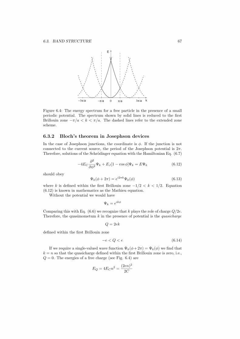
6.3. BAND STRUCTURE 67
π/a−π/a 3π/a−3π/a 0 k
E
Figure 6.4: The energy spectrum for a free particle in the presence of a smallperiodic potential. The spectrum shown by solid lines is reduced to the firstBrillouin zone −π/a < k < π/a. The dashed lines refer to the extended zonescheme.
6.3.2 Bloch’s theorem in Josephson devices
In the case of Josephson junctions, the coordinate is φ. If the junction is notconnected to the current source, the period of the Josephson potential is 2π.Therefore, solutions of the Schrodinger equation with the Hamiltonian Eq. (6.7)
−4EC∂2
∂φ2Ψk + EJ [1 − cosφ]Ψk = EΨk (6.12)
should obeyΨk(φ+ 2π) = ei2πkΨk(φ) (6.13)
where k is defined within the first Brillouin zone −1/2 < k < 1/2. Equation(6.12) is known in mathematics as the Mathieu equation.
Without the potential we would have
Ψk = eikφ
Comparing this with Eq. (6.6) we recognize that k plays the role of charge Q/2e.Therefore, the quasimometum k in the presence of potential is the quasicharge
Q = 2ek
defined within the first Brillouin zone
−e < Q < e (6.14)
If we require a single-valued wave function Ψk(φ+2π) = Ψk(φ) we find thatk = n so that the quasicharge defined within the first Brillouin zone is zero, i.e.,Q = 0. The energies of a free charge (see Fig. 6.4) are
EQ = 4ECn2 =
(2en)2
2C
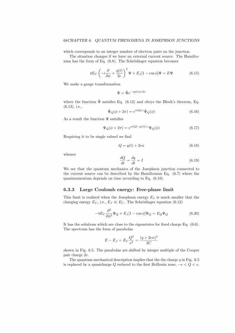
68CHAPTER 6. QUANTUM PHENOMENA IN JOSEPHSON JUNCTIONS
which corresponds to an integer number of electron pairs on the junction.The situation changes if we have an external current source. The Hamilto-
nian has the form of Eq. (6.8). The Schrodinger equation becomes
4EC
(−i ∂∂φ
+q(t)2e
)2
Ψ + EJ [1 − cosφ]Ψ = EΨ (6.15)
We make a gauge transformation
Ψ = Ψe−iq(t)φ/2e
where the function Ψ satisfies Eq. (6.12) and obeys the Bloch’s theorem, Eq.(6.13), i.e.,
ΨQ(φ+ 2π) = eiπQ/eΨQ(φ) (6.16)
As a result the function Ψ satisfies
ΨQ(φ+ 2π) = eiπ[Q−q(t)]/eΨQ(φ) (6.17)
Requiring it to be single valued we find
Q = q(t) + 2en (6.18)
whencedQ
dt=dq
dt= I (6.19)
We see that the quantum mechanics of the Josephson junction connected tothe current source can be described by the Hamiltonian Eq. (6.7) where thequasimomentum depends on time according to Eq. (6.19).
6.3.3 Large Coulomb energy: Free-phase limit
This limit is realized when the Josephson energy EJ is much smaller that thecharging energy EC , i.e., EJ � EC . The Schrodinger equation (6.12)
−4EC∂2
∂φ2ΨQ + EJ [1 − cosφ]ΨQ = EQΨQ (6.20)
It has the solutions which are close to the eigenstates for fixed charge Eq. (6.6).The spectrum has the form of parabolas
E − EJ = ECQ2
e2=
(q + 2en)2
2C
shown in Fig. 6.5. The parabolas are shifted by integer multiple of the Cooperpair charge 2e.
The quantum-mechanical description implies that the the charge q in Fig. 6.5is replaced by a quasicharge Q reduced to the first Brillouin zone, −e < Q < e.
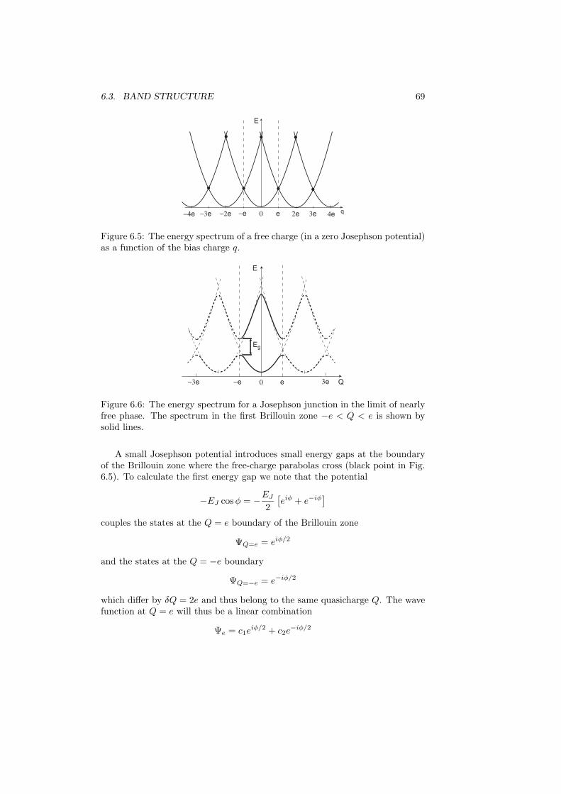
6.3. BAND STRUCTURE 69
e 3e−3e 0 q
E
2e−2e −e 4e−4e
Figure 6.5: The energy spectrum of a free charge (in a zero Josephson potential)as a function of the bias charge q.
e−e 3e−3e 0 Q
E
Eg
Figure 6.6: The energy spectrum for a Josephson junction in the limit of nearlyfree phase. The spectrum in the first Brillouin zone −e < Q < e is shown bysolid lines.
A small Josephson potential introduces small energy gaps at the boundaryof the Brillouin zone where the free-charge parabolas cross (black point in Fig.6.5). To calculate the first energy gap we note that the potential
−EJ cosφ = −EJ
2[eiφ + e−iφ
]couples the states at the Q = e boundary of the Brillouin zone
ΨQ=e = eiφ/2
and the states at the Q = −e boundary
ΨQ=−e = e−iφ/2
which differ by δQ = 2e and thus belong to the same quasicharge Q. The wavefunction at Q = e will thus be a linear combination
Ψe = c1eiφ/2 + c2e
−iφ/2
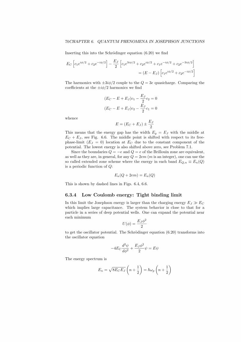
70CHAPTER 6. QUANTUM PHENOMENA IN JOSEPHSON JUNCTIONS
Inserting this into the Schrodinger equation (6.20) we find
EC
[c1e
iφ/2 + c2e−iφ/2
]− EJ
2
[c1e
3iφ/2 + c2eiφ/2 + c1e
−iφ/2 + c2e−3iφ/2
]= (E − EJ)
[c1e
iφ/2 + c2e−iφ/2
]The harmonics with ±3iφ/2 couple to the Q = 3e quasicharge. Comparing thecoefficients at the ±iφ/2 harmonics we find
(EC − E + EJ )c1 −EJ
2c2 = 0
(EC − E + EJ )c2 −EJ
2c1 = 0
whenceE = (EC + EJ) ± EJ
2This means that the energy gap has the width Eg = EJ with the middle atEC + EJ , see Fig. 6.6. The middle point is shifted with respect to its free-phase-limit (EJ = 0) location at EC due to the constant component of thepotential. The lowest energy is also shifted above zero, see Problem 7.1.
Since the boundaries Q = −e and Q = e of the Brillouin zone are equivalent,as well as they are, in general, for any Q = 2em (m is an integer), one can use theso called extended zone scheme where the energy in each band EQ,n ≡ En(Q)is a periodic function of Q:
En(Q+ 2em) = En(Q)
This is shown by dashed lines in Figs. 6.4, 6.6.
6.3.4 Low Coulomb energy: Tight binding limit
In this limit the Josephson energy is larger than the charging energy EJ � EC
which implies large capacitance. The system behavior is close to that for aparticle in a series of deep potential wells. One can expand the potential neareach minimum
U(φ) =EJφ
2
2to get the oscillator potential. The Schrodinger equation (6.20) transforms intothe oscillator equation
−4ECd2ψ
dφ2+EJφ
2
2ψ = Eψ
The energy spectrum is
En =√
8ECEJ
(n+
12
)= hωp
(n+
12
)

6.4. COULOMB BLOCKADE 71
φ
U
Eb
Ψ
0 2π−2π
Figure 6.7: The energy band spectrum for a Josephson junction in the limit oflarge Josephson energy (tight binding). The energy bands are widened oscillatorlevels for a localized particle with the wave function ψ.
The energy spacing hωp ∼ EJ
√EC/EJ � EJ . The lowest energy wave function
is
ψ0(φ) = C exp
(−φ
2
4
√EJ
2EC
)
Due to the periodic nature of the potential one can construct the true wavefunction
ΨQ,n(φ) =∑m
ei2πm(Q/2e)Ψn(φ− 2πm)
where Ψn(φ− 2πm) is a function centered at φ = 2πm. The function Ψn(φ) iscalled the Wannier function [11]. It is close to the wave function ψn(φ) obtainedby solving the equation near each minimum. This wave function ΨQ,n(φ) sat-isfies the Bloch condition Eq. (6.16). Each level is broadened into an energyband (see Problem 7.3)
EQ = En − 12Eb,n cos
πQ
e(6.21)
The band width is determined by overlaps of the wave functions Ψn(φ) centeredat φm = 2πm. It is exponentially small. For example, the lowest band width is
Eb,0 = 32(EJEC
π
)1/2(EJ
2EC
)1/2
exp
(−√
8EJ
EC
)
The quantum properties of Josephson junctions are discussed in review [?].
6.4 Coulomb blockade
Let us consider Fig. 6.5. If we increase, by a bias current from the externalsource, the charge starting from q = 0 for n = 0 the energy will increase untilit reaches the crossing point (black dot) at q = e corresponding to the chargee on the capacitor and to the voltage e/C across the capacitor. With a furtherincrease in q the system will go over to a state with n = −1 corresponding tothe parabola shifted by 2e to the right that has a lower energy. The transitionfrom n = 0 to n = −1 corresponds to the 2e charge transfer through the

72CHAPTER 6. QUANTUM PHENOMENA IN JOSEPHSON JUNCTIONS
tunnel Josephson junction. We see that the charge transfer (current) throughthe capacitor occurs only when the voltage reaches a threshold value VC = e/C.This is the Coulomb blockade: preventing of the charge transfer by the chargingenergy. To describe the Coulomb blockade quantum-mechanically, we need firstto consider the semi-classical equation of motion in a periodic potential.
6.4.1 Equation of motion
In the semi-classical theory than neglects transition between energy bands, theequation of motion for the quasimomentum of a particle is [11]
h∂k
∂t= F
For a constant force F this gives hk = Ft. The velocity is
∂x
∂t=∂En
h∂k
where En(k) is the band energy. This yields
∂x
h∂k=
1F
∂En
h∂k
orx = F−1En(k) , hk = Ft
For a free particle in zero potential E(k) = h2k2/2m, so that the particle iscontinuously accelerated. However, in a periodic potential, E(k) is a periodicfunction. Therefore, instead of being accelerated, the coordinate of particleperforms Bloch oscillations with the amplitude Δx = 2Eb/F and a period
t =2πhaF
In a first Brillouin zone picture, the particle is moving until it is reflectedat the zone boundary such that its quasimomentum changes from kB = π/a atone boundary to kB − 2π/a = −kB at another boundary.
6.4.2 Bloch oscillations and the Coulomb blockade in Joseph-son junctions
Consider low currents such that the (Zener) transitions from one band to anotherhave low probability. In a Josephson junction, the force equation has the form
∂Q
∂t= I (6.22)
while∂φ
∂t=∂EQ,n
h∂k=
2eh
∂EQ,n
∂Q(6.23)

6.4. COULOMB BLOCKADE 73
e−e 3e−3e 0 Q
E
Eg
Q = I.
ZenerBloch
Figure 6.8: The Bloch oscillations are reflections of a particle from the Brillouinzone boundaries within one energy band. The Zener transitions between thebands lead to semiclassical behavior.
Therefore, for a constant current,
∂φ
∂Q=
2eIh
∂EQ,n
∂Q
so thatφ =
2eIhEn(Q)
The period of Bloch oscillations is from Eq. (6.22)
tB =2eI
The amplitude of Bloch oscillations is
Δφ =2eIhEb
In the limit of large Coulomb energy (free phase), EC � EJ
Eb ≈ EC
andΔφ ≈ 2eEC/Ih ∼ tB/R0C � 1
The phase is not fixed: it oscillates rapidly with a large amplitude. The voltageis
V =h
2e∂φ
∂t=∂EQ,n
∂Q≈ Q
C

74CHAPTER 6. QUANTUM PHENOMENA IN JOSEPHSON JUNCTIONS
e/C
-e/C
V
t
Figure 6.9: The voltage across the junction as a function of time for a constantcurrent bias.
φ
U
Eb
0 2π−2π
Figure 6.10: MQT is equivalent to Landau–Zener transitions between the energybands up to the continuum. The energy bands are widened oscillator levels fora localized particle with the wave function ψ.
Each time when the quasicharge Q approaches the boundary of the Brillouinzone QB = +e (or QB = −e), the quasicharge changes QB → QB ±2e such thatthe voltage jumps from +e/C to −e/C (or vice versa). The average voltage iszero.
The change in the quasicharge Q by 2e means the 2e charge transfer throughthe Josephson junction. We see that the charge transfer through the junctionoccurs only when the voltage across the junction reaches a threshold value e/C.This is the quantum-mechanical picture of the Coulomb blockade. The chargingenergy of the junction prevents the charge transfer through it unless the voltageexceeds the threshold. At the threshold VC = e/C, the charging energy Q2/2Cof a charge Q = e becomes equal to the charging energy (Q − 2e)2/2C of thecharge Q = e − 2e = −e on the capacitor after the Cooper pair has tunnelledthrough the junction. To see the Coulomb blockade one needs a junction witha rather low capacity.
On the contrary, if the capacity is high such that EJ � EC , the band widthis very narrow, and the amplitude of phase oscillations is exponentially small.The phase is essentially fixed such that the current Ic cosφ flows without voltage:the junction is superconducting. A finite voltage can then appear as a result ofmacroscopic quantum tunnelling considered in the previous Section within thesemiclassical approach. In the semiclassical picture of Eqs. (6.22) and (6.23),the macroscopic quantum tunnelling is equivalent to Zener transitions from alower band up to higher bands in Fig. 6.7 and finally to the continuum forE > EJ (see Fig. 6.10). Neglecting the Zener transitions implies absence ofMQT and assumes that the bias current is small.
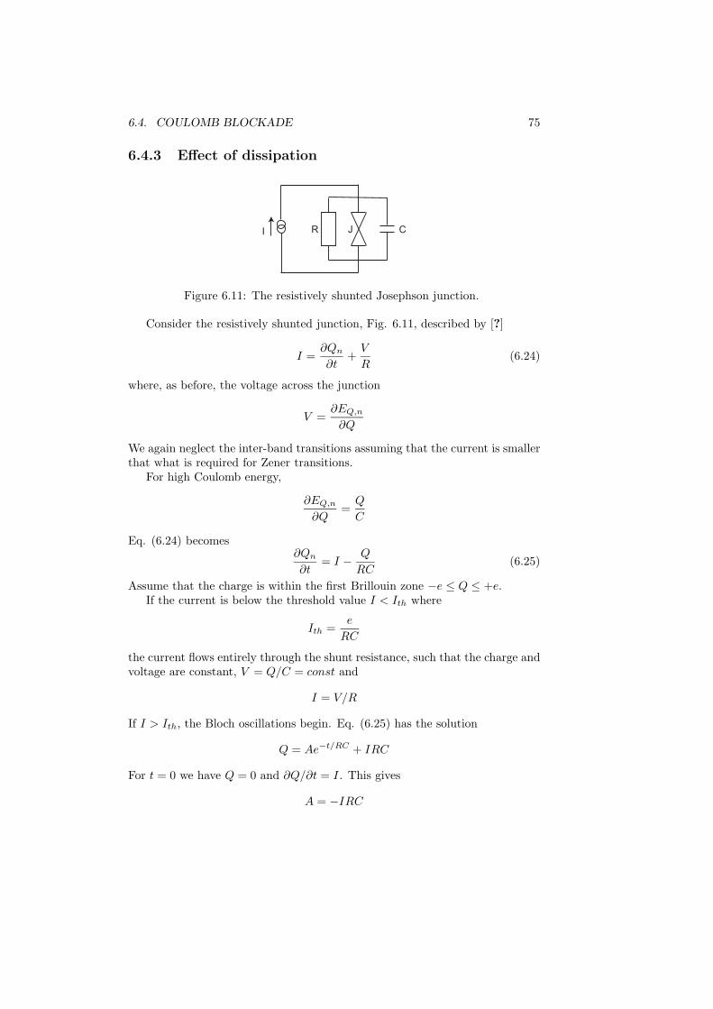
6.4. COULOMB BLOCKADE 75
6.4.3 Effect of dissipation
R J CI
Figure 6.11: The resistively shunted Josephson junction.
Consider the resistively shunted junction, Fig. 6.11, described by [?]
I =∂Qn
∂t+V
R(6.24)
where, as before, the voltage across the junction
V =∂EQ,n
∂Q
We again neglect the inter-band transitions assuming that the current is smallerthat what is required for Zener transitions.
For high Coulomb energy,
∂EQ,n
∂Q=Q
C
Eq. (6.24) becomes∂Qn
∂t= I − Q
RC(6.25)
Assume that the charge is within the first Brillouin zone −e ≤ Q ≤ +e.If the current is below the threshold value I < Ith where
Ith =e
RC
the current flows entirely through the shunt resistance, such that the charge andvoltage are constant, V = Q/C = const and
I = V/R
If I > Ith, the Bloch oscillations begin. Eq. (6.25) has the solution
Q = Ae−t/RC + IRC
For t = 0 we have Q = 0 and ∂Q/∂t = I. This gives
A = −IRC

76CHAPTER 6. QUANTUM PHENOMENA IN JOSEPHSON JUNCTIONS
V/Vth
I/Ith
1
1
Figure 6.12: The d.c. I-V curve for resistively shunted quantum junction forthe limit of high Coulomb energy. Vth = IthR = e/C.
Assume that at t = −t1 the charge was at the end Q = −e of the Brillouin zone,while at t = t2 the charge was at the end Q = +e of the Brillouin zone. We find
A exp(−t2/RC) = e− IRC , A exp(t1/RC) = −e− IRC
Therefore
exp(t1 + t2RC
)=IRC + e
IRC − e
The average voltage is found from
(t1 + t2)V
R=∫ t2
−t1
[A
RCexp
(− t
RC
)+ I
]dt
= (t1 + t2)(I +
A
t1 + t2[exp(t1/RC) − exp(−t2/RC)]
)
Finally,V
R= I − 2Ith
[lnI + IthI − Ith
]−1
The second term is zero for I − Ith and diverges for I → ∞. The I-V curve isshown in Fig. 6.12. The maximum d.c. voltage V is Vth = IthR = e/C. ForR→ ∞ the I-V curve is vertical which means zero d.c. voltage.
6.5 Parity effects
Let us consider a junction in Fig. 6.1 made of normal conductors and studyhow its properties change when a superconducting gap is introduced.

6.5. PARITY EFFECTS 77
e/2−e/2 3e/2−3e/2 0 q
E
e 2e−2e −e
Figure 6.13: The e-periodic energy dependence of a normal junction as a func-tion of the continuous charge q supplied by the external source.
In the case of a normal junction, the wave function depends on a single-electron phase φ1 = φ/2 such that the charge operator in Eq. (6.5) becomes
Q = −2ie∂
∂φ= −ie ∂
∂φ1(6.26)
The eigenfunction has the form
ΨQ = eiQφ1/e
which is 2π-periodic for Q = ne. The Josephson current disappears, and theHamiltonian becomes
H = −EC∂2
∂φ21
If the junction is connected to the external leads, the Hamiltonian takes theform
H = EC
(−i ∂
∂φ1+q(t)e
)2
The solution of the corresponding Schrodinger equation has the form
Ψ = ei(Q−q)φ1/e
The condition of 2π-periodicity gives Q = q +me where m is an integer.The energy is
EQ = ECQ2
e2= EC
(q +me)2
e2
It is shown in Fig. 6.13. The different parabolas correspond to different valuesof m.
Assume we start with m = 0. As we increase the charge q supplied by theexternal source, the energy grows until q reaches e/2 which corresponds to thevoltage VC = e/2C. At this moment, the energy of the capacitor becomes equalto the energy for the state with m = −1, i.e., to (q − e)2/2C. At this point thecharge at the capacitor decreases by e, one electron being transferred through

78CHAPTER 6. QUANTUM PHENOMENA IN JOSEPHSON JUNCTIONS
0 q
E
e 2e−2e −e
0 q
E
e 2e−2e −e
0 q
E
e 2e−2e −e
EC
EC
Δ
Δ
(a)
(b)
(c)
Figure 6.14: The energy of junctions. (a) e-periodic dependence in the normalstate. (b) Energy of odd-number states is shifted by Δ < EC . The chargetransfer occurs at the crossing points (black dots). (c) Δ > EC , the chargetransfer occurs with a 2e periodicity.
the junction via tunnelling. We see again that the charge transfer (current) doesnot occur unless voltage reaches the threshold value VC (Coulomb blockade).
Consider again the device shown in Fig. 6.1 and apply a gate voltage VG
between the island and the gate electrode. If VG = VC , the energy of thejunction corresponds to the level where the parabolas cross (black dots in Fig.6.13). This means that an infinitely small voltage V can lead to a continuoustransfer of charge from lead L1 to lead L2.
Let us now assume that the island I is superconducting with an energy gapΔ. For simplicity we restrict ourselves to zero temperatures. If the numberof electrons on it is even, they all are included into Cooper pairs and formthe ground state with zero energy plus the charging energy. If now we add anextra (odd) particle, it can only occupy a state above the gap thus the energywill be Δ plus the charging energy. One more particle will make a pair withthe previous one thus decreasing the total energy down to simply the chargingenergy. Therefore, the states with odd number of particles will have energywhich is the charging energy for the given number of particles shifted by +Δwith respect to the energy for the even number of particles. This is shown inFig. 6.14.
Shift of the parabolas for odd particle numbers destroys the e-periodicityof the energy spectrum. When Δ becomes larger than the charging energyΔ > EC , the charge transfer occurs only within the states with even number of
6.5. PARITY EFFECTS 79
particles, and the 2e-periodicity characteristic for a superconducting system isrestored (Fig. 6.14(c)).
When also the leads become superconducting, the Josephson energy appears,and the gaps open at the crossing points shown by black dots. The energy depen-dence returns to Fig. 6.6 for a superconducting Josephson junction consideredbefore.
80CHAPTER 6. QUANTUM PHENOMENA IN JOSEPHSON JUNCTIONS
Bibliography
[1] P.G. de Gennes Superconductivity of Metals and Alloys (W.A. Benjamin,Inc, 1965).
[2] M. Tinkham, Introduction to superconductivity (McGraw-Hill, New York,1996).
[3] J. Bardeen, L.N. Cooper, and J.R. Schrieffer, Phys. Rev. 108, 1175 (1957).
[4] L.D. Landau and E.M. Lifshitz, Statistical Physics Part 2: Theory of thecondensed state, by E.M. Lifshitz and L.P. Pitaevskii (Pergamon, Oxford1980), Chapter III.
[5] Abrikosov, A. A. Fundamentals of The Theory of Metals. (North Holland,Amsterdam, 1998).
[6] D. Saint-James, G. Sarma, and E.J. Thomas Type II superconductivity(Pergamon Press, 1969).
[7] R. Feynman, in: Progress in Low Temperature Physics vol. 1, edited by C.J. Gorter (North Holland, Amsterdam, 1955) p. 36.
[8] A.A. Abrikosov, Zh. Eksp. Teor. Fiz. 32, 1442 (1957) [Sov. Phys. JETP 5,1174 (1957)].
[9] A. F. Andreev, Zh. Eksp. Teor. Fiz. 49, 655 (1965) [Sov. Phys. JETP 22,455 (1966)].
[10] G.E. Blonder, M. Tinkham, and T.M. Klapwijk, Phys. Rev. B, 25, 4515(1982).
[11] J.M. Ziman, Principles of the theory of solids, (Cambrgidge UniversityPress, 1965).
[12] D.V. Averin and K.K. Likharev, “Single Electronics: Correlated Transfer ofSingle Electrons and Cooper Pairs in Systems of Small Tunnel Junctions”,in: Mesoscopic Phenomena in Solids, B.I. Altshuler, P.A. Lee, and R.A.Webb, eds. (Elsevier, New York 1991), p. 169.
81
82 BIBLIOGRAPHY
[13] G.-L. Ingold and Yu. V. Nazarov, “Charge tunneling rates in ultrasmalljunctions”, in: Single Charge Tunneling”, H. Grabert and M.H. Devoret,eds., NATO ASI Series, Vol. 294, pp. 21–107 (Plenum Press, New York,1992); arXiv:cond-mat/0508728v1
[14] J.P. Pekola, K.P. Hirvi, J.P. Kauppinen, and M.A. Paalanen, Phys. Rev.Lett. 94, 2903 (1994).
[15] Yu. V. Nazarov and Ya. M. Blanter, Quantun Transport (Cambridge Uni-versity Press, 2009).