Hidden symmetries of dynamics in classical and quantum physics


Introduction to the Standard ModelMEXICOPAS 2019
Mauro Napsuciale
Departamento de Fısica, Universidad de Guanajuato, Mexico
Leon, Gto., June 2019
Outline
1 FundamentalsSymmetries in Classical and Quantum Mechanics.Irreducible representations (irreps) of SU(2).Irreps of the HLG: Chirality, Parity and Dirac Equation.Quantum Field theory: complex scalar field.
2 Electroweak interactions: Glashow-Weinberg-Salam theory.Minimal coupling principle in classical mechanics.Gauge theories: Abelian and non-Abelian.Quantum ElectrodynamicsFermi theory, IVB theory, parity violation and V-A structure ofweak interactionsGWS Theory. Spontaneous Breaking of Symmetries.
3 Strong interactions:QCD.Irreducible representations of SU(3)Classification of hadrons: Eightfold Way, Quark ModelGauge theory of strong interactions: QCD.Running of couplings: Confinement and asymptotic freedom.Experimental evidence for color degrees of freedom.
What these lectures are...
In these lectures I will give an introduction to :1 What is an elementary particle? Quantum realm. Symmetries.
Group theory.2 How do we describe their electromagnetic, weak and strong
interactions?3 No time for a historical account on how we arrived at the SM.
Fascinating story of hundreds of experiments, a plethora ofideas and more than 40 Nobel prizes during the last century.
4 The most impressive intelectual construction of human kindso far in my opinion.
5 Overconstrained framework after the discovery of the Higgs,but not the end of the story. Many things to do in HEP.
6 Most of the previously explored routes are not appealing now,but new challenges in HEP: neutrinos, dark matter,matter-antimatter asymmetry (CP violation), dark energy.Quantum theory of gravity.
The magic word in physics is...
S Y M M E T R YYou must master the natural language of
symmetries: group theory.
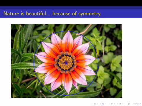
Nature is beautiful... because of symmetry.

Nature is beautiful... because of symmetry (d ≈ 10−20m).
34*,5 . 34*,6 . 4*,7
3, 5%M6
E8
4 2
F/F"
F/"//F"
/"
Standard Model of Particle Interactions
Quantum theory of electromagnetic, weak and stronginteractions of the known elementary particles.
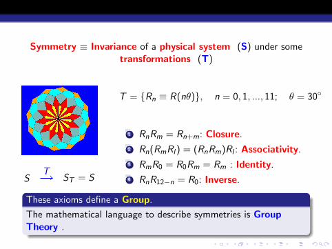
Symmetry ≡ Invariance of a physical system (S) under sometransformations (T)
S ST = ST
T = Rn ≡ R(nθ), n = 0, 1, ..., 11; θ = 30
1 RnRm = Rn+m: Closure.
2 Rn(RmRl) = (RnRm)Rl : Associativity.
3 RmR0 = R0Rm = Rm : Identity.
4 RnR12−n = R0: Inverse.
These axioms define a Group.
The mathematical language to describe symmetries is GroupTheory .
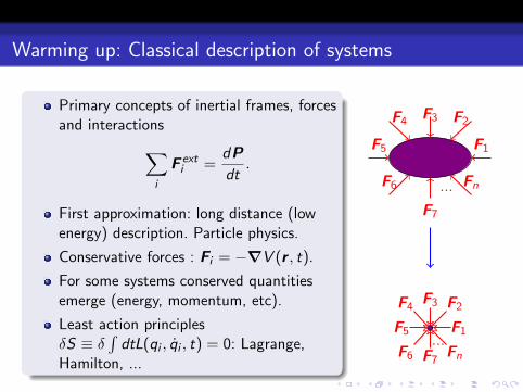
Warming up: Classical description of systems
Primary concepts of inertial frames, forcesand interactions∑
i
F exti =
dPdt.
First approximation: long distance (lowenergy) description. Particle physics.
Conservative forces : Fi = −∇V (r , t).
For some systems conserved quantitiesemerge (energy, momentum, etc).
Least action principlesδS ≡ δ
∫dtL(qi , qi , t) = 0: Lagrange,
Hamilton, ...
F1
F2F3F4
F5
F6
F7
... Fn
F1
F2F3F4
F5
F6 F7
...Fn
Symmetries in classical mechanics.
A guide to the most convenient choice of generalizedcoordinates, e.g. solution to the central potential V = V (r) iseasier taking q1 = r , q2 = θ, q3 = φ.
Independence of V on some generalized coordinate is asymmetry of the system.
These symmetries yield a conserved quantities
pi =∂L
∂qi.
Systematics: Emily Noether, 1915
Symmetries of S =∫dtL(qi , qi , t) ⇔ conserved quantities

Symmetries and conserved quantities: Noether’s theorem
Simplest version: symmetries of L
In the Lagrange formalism
L =∑i
1
2mq2
i − V (qi , t)
Perform a transformation∆qi
∆L =∂L
∂qi∆qi +
∂L
∂qi∆qi
=d
dt(∂L
∂qi)∆qi +
∂L
∂qi∆qi
=d
dt(∂L
∂qi∆qi ).
If L is invariant (∆L = 0)⇒ ∂L
∂qi∆qi = cte.
Continuous transformationscan be written in terms ofsome independentparameters εk
∆qi =∑k
εkξik(q, q)
Conserved Noether charges
Qk =∂L
∂qiξik(q, q).

Space translations :
δqi = εkδik ⇒ Qk =∂L
∂qiδik =
∂L
∂qk≡ pk
Rotations
r′
rδθ
δr
n
δr = n × rδθδxi = εiklnkxlδθ,
ξik = εiklxl , εk = nkδθ
⇒ Qk =∂L
∂xiεiklxl = (r × p)k = Lk
Solving the classical dynamics of a particle amounts to find all thesymmetries of the system
But elementary particles live in the Quantum Realm

In preparation: Rotations and the exponential map.
r′
rdθ
dr
n
dr = n × rdθ
x ′i = xi + εijknjxkdθ
= (δik + εijknjdθ)xk
= (δik − i(J · n)ikdθ)xk
(Ji )jk = −iεijk
Classical mechanics
Finite rotations (dθ ↔ θN )
r ′ = R(n, θ)r ,
R(n, θ) = lımN→∞
(13×3 − i(J · n)θ
N)N
= e−iJ·n θ.
R depend continuously on threeparameters θ = nθ.
J ≡ Rotation generators in R3
3× 3 matrices satisfying
[Ji , Jj ] = iεijkJk

J are Hermitian matrices of null trace
((Ji )†)jk = (−iεikj)∗ = −iεijk = (Ji )jk
Tr(Ji ) = −iεijj = 0
Rotation operators are orthogonal matrices
[R(n, θ)]t = [e−iJ·n θ]t = e−iJt ·nθ = e+iJ·nθ = [R(n, θ)]−1,
with unit determinant
Det[R(n, θ)] = Det[e−iJ·n θ] = e−iTr(J)·n = 1.
Rotation operators in classical mechanics (R3) form a groupwith the conventional matrix product
Group of 3× 3 orthogonal matrices of unit determinant ≡ SO(3)group. Fully characterized by the Lie algebra
[Ji , Jj ] = iεijkJk
Elementary particles live in the Quantum Realm

Quantum Mechanics in a nutshell
1 Physical information of the system encoded in the state vector|ψ〉 ∈ H.
2 Observables represented by hermitian operators acting on H 1.3 A measurement of the observable A can only yield one of the
eigenvalues ak of the representing operador (A|ai 〉 = ai |ai 〉).4 Before measuring A we don’t know with certainty the
resulting eigenvalue ak , we only know the probability
P(ak) = |〈ak |ψ〉|2.
5 If the resulting value of a measurement of A is am, the statedescribing the system immediately after is |am〉.
6 Dynamics is dictated by the Schrodinger equation
i~∂t |ψ(t)〉 = H|ψ(t)〉.1The eigenvalues of a Hermitian operators are real numbers.

Characterizing the Hilbert space
We need a complete set of commuting observables (CSCO).We always choose H in this set ≡ H,A,B,C ....Common eigenstates |E , a, b, c , ...〉 form a basis of H.
S
H
Eabcd...
The eigenvalues of the CSCO, E , a, b, c ... are referred to asgood quantum numbers.All operators in the CSCO conmute with H:
[H,A] = [H,B] = [H,C ] = ... = 0.
They represent conserved quantities.
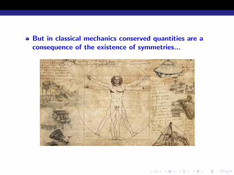
But in classical mechanics conserved quantities are aconsequence of the existence of symmetries...
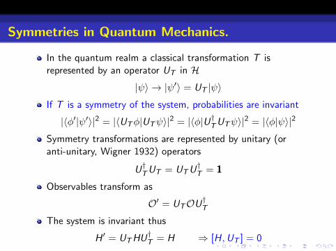
Symmetries in Quantum Mechanics.
In the quantum realm a classical transformation T isrepresented by an operator UT in H
|ψ〉 → |ψ′〉 = UT |ψ〉If T is a symmetry of the system, probabilities are invariant
|〈φ′|ψ′〉|2 = |〈UTφ|UTψ〉|2 = |〈φ|U†TUTψ〉|2 = |〈φ|ψ〉|2
Symmetry transformations are represented by unitary (oranti-unitary, Wigner 1932) operators
U†TUT = UTU†T = 1
Observables transform as
O′ = UTOU†TThe system is invariant thus
H ′ = UTHU†T = H ⇒ [H,UT ] = 0

If the symmetry is continuous UT can always be written in aexponential form (exponential map)
UT = e iG with G † = G .
Continuous transformations depend on n parametrosαi , i = 1, 2, ...n. e.g. for SO(3), αi = θi .There are n generators Gi (e.g. for SO(3), Gi = Ji ). Ingeneral G = Giαi = G ·α.The generators of continuous symmetries are Hermitianoperators. Represent observables in QM.[UT ,H] = 0⇒ [Gi ,H] = 0. Generators of continuoussymmetries are natural candidates for the CSCO.Only those generators commuting with each other canbe in the CSCO : Cartan Sub-algebra of the symmetrygroup.In addition there are products of generators commuting withall Gi : Casimir Operators of the symmetry group. Theyalso belong to the CSCO.

Conclusion: a quantum system is fully characterized by itstotal symmetry group
Good quantum numbers correspond to the eigenvalues of H, theCasimir operators of the full symmetry group and the generators inthe Cartan sub-algebra of this group. Quantum states are classifiedinto minimal subspaces invariant under the full symmetry grouptransformations (irreducible representaciones, irreps for short).
Elementary particles are quantum systems. We must find andclassify all their symmetries:
1 Free particles: Space-time symmetries. Poincare group:Rotations+translations+boosts. Supersymmetry?
2 Interacting particles: Gauge symmetries:SU(3)c ⊗ SU(2)L ⊗ Y (1)Y .
3 Global symmetries: lepton number, baryon number etc.
4 Discrete symmetries: C , P, T , CP, PT , CPT , etc.
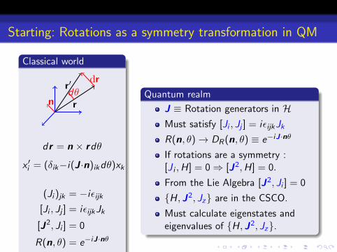
Starting: Rotations as a symmetry transformation in QM
Classical world
r′
rdθ
dr
n
dr = n × rdθ
x ′i = (δik−i(J ·n)ikdθ)xk
(Ji )jk = −iεijk[Ji , Jj ] = iεijkJk
[J2, Ji ] = 0
R(n, θ) = e−iJ·nθ
Quantum realm
J ≡ Rotation generators in HMust satisfy [Ji , Jj ] = iεijkJk
R(n, θ)→ DR(n, θ) ≡ e−iJ·nθ
If rotations are a symmetry :[J i ,H] = 0⇒ [J2,H] = 0.
From the Lie Algebra [J2, Ji ] = 0
H, J2, Jz are in the CSCO.
Must calculate eigenstates andeigenvalues of H, J2, Jz.
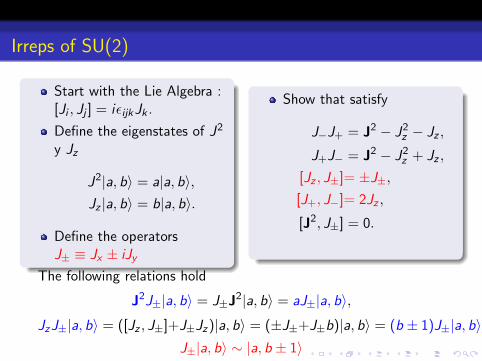
Irreps of SU(2)
Start with the Lie Algebra :[Ji , Jj ] = iεijkJk .
Define the eigenstates of J2
y Jz
J2|a, b〉 = a|a, b〉,Jz |a, b〉 = b|a, b〉.
Define the operatorsJ± ≡ Jx ± iJy
Show that satisfy
J−J+ = J2 − J2z − Jz ,
J+J− = J2 − J2z + Jz ,
[Jz , J±]= ±J±,[J+, J−]= 2Jz ,
[J2, J±] = 0.
The following relations hold
J2J±|a, b〉 = J±J2|a, b〉 = aJ±|a, b〉,
JzJ±|a, b〉 = ([Jz , J±]+J±Jz)|a, b〉 = (±J±+J±b)|a, b〉 = (b ± 1)J±|a, b〉J±|a, b〉 ∼ |a, b ± 1〉
Use the last relation k times
(J±)k |a, b〉 ∼ |a, b ± k〉
But
J2 − J2z =
1
2(J+J− + J−J+) =
1
2
(J+(J+)† + (J+)†J+
)thus
〈a, b|J2 − J2z |a, b〉 =
1
2(〈a, b|J+(J+)†|a, b〉+ 〈a, b|(J+)†J+|a, b〉)
=1
2(||J†+|a, b〉||+ ||J+|a, b〉||) > 0
hencea− b2 > 0⇒ b2 ≤ a.
There must exist bmax y bmın such that
J+|a, bmax〉 = 0 J−|a, bmın〉 = 0

From these relations
J−J+|a, bmax〉 = 0 ⇒ (J2 − J2z − Jz)|a, bmax〉 = 0
a− b2max − bmax = 0⇒ a = bmax(bmax + 1).
Also
J+J−|a, bmın >= (J2 − J2z + Jz)|a, bmın〉 = 0
soa = bmın(bmın − 1).
Finally
bmax(bmax + 1) = bmın(bmın − 1) ⇒ bmax = −bmın.
Furthermore, for some integer n
(J+)n|a, bmın〉 ∼ |a, bmax〉.
bmax = bmın + n⇒ bmax =n
2⇒ a =
n
2(n
2+ 1)

Define j ≡ n2 such that bmax = j y a = j(j + 1). On the other
side bmın = −j and bmax − bmın = n, hence b = m wherem = −j ,−j + 1, ..., j − 1, j .In this notation
J2|j ,m〉 = j(j + 1)|j ,m〉, Jz |j ,m〉 = m|j ,m〉As to the raising operator
J+|jm〉 = Cjm|j ,m + 1〉.But
〈jm|(J+)†J+|jm〉 = |Cjm|2 = 〈jm|J2−J2z−Jz |jm〉 = [j(j+1)−m(m+1)]
Assuming real coefficients (Condon-Shortley convention)
|Cjm| =√j(j + 1)−m(m + 1) =
√(j −m)(j + m + 1)
J+|j ,m〉=√
(j −m)(j + m + 1)|j ,m + 1〉Similarly
J−|j ,m〉 =√
(j + m)(j −m + 1)|j ,m − 1〉

Summarizing: irreps de SU(2)
J2|j ,m〉 = j(j + 1)|j ,m〉Jz |j ,m〉 = m|j ,m〉
J±|j ,m〉 =√
(j ∓m)(j ±m + 1)|j ,m ± 1〉
j =n
2,
m = −j ,−j + 1, .., j .
mj = 0 :
0
mj = 12 :
−12
12
mj = 1 :
−1 0 1
mj = 32 :
−12
12−3
232
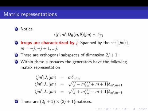
Matrix representations
1 Notice〈|j ′,m′|DR(n, θ)|jm〉 ∼ δj ′j
2 Irreps are characterized by j . Spanned by the set|jm〉,m = −j ,−j + 1, ...j .
3 These are orthogonal subspaces of dimension 2j + 1.
4 Within these subspaces the generators have the followingmatrix representation
〈jm′|Jz |jm〉 = mδm′m
〈jm′|J+|jm〉 =√
(j −m)(j + m + 1)δm′,m+1
〈jm′|J−|jm〉 =√
(j + m)(j −m + 1)δm′,m−1
5 These are (2j + 1)× (2j + 1)matrices.

Defining representation: j = 12
mj = 12 :
−12
12
Shorthand notation: |12 ,−12〉 ≡ |−〉, |
12 ,
12〉 ≡ |+〉.
J−|−〉 = 0, J−|+〉 = |−〉, J+|−〉 = |+〉, J+|+〉 = 0.
Matrix representation for j = 12
〈jm′|Jz |jm〉 =
(〈+|Jz |+〉 〈+|Jz |−〉〈−|Jz |+〉 〈−|Jz |−〉
)=
1
2
(1 00 −1
)≡ 1
2σz ,
〈jm′|J+|jm〉 =
(〈+|J+|+〉 〈+|J+|−〉〈−|J+|+〉 〈−|J+|−〉
)=
1
2
(0 10 0
)≡ 1
2σ+,
〈jm′|J−|jm〉 =
(〈+|J−|+〉 〈+|J−|−〉〈−|J−|+〉 〈−|J−|−〉
)=
1
2
(0 01 0
)≡ 1
2σ−.
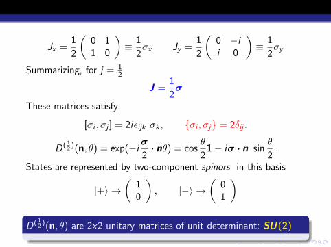
Jx =1
2
(0 11 0
)≡ 1
2σx Jy =
1
2
(0 −ii 0
)≡ 1
2σy
Summarizing, for j = 12
J =1
2σ
These matrices satisfy
[σi , σj ] = 2iεijk σk , σi , σj = 2δij .
D( 12
)(n, θ) = exp(−i σ2· nθ) = cos
θ
21− iσ · n sin
θ
2.
States are represented by two-component spinors in this basis
|+〉 →(
10
), |−〉 →
(01
)
D( 12
)(n, θ) are 2x2 unitary matrices of unit determinant: SU(2)

Adjoint representation: j = 1
mj = 1 :
−1 0 1
A similar calculation yields
Jx =
0 1√2
01√2
0 1√2
0 1√2
0
, Jy =
0 − i√2
0i√2
0 − i√2
0 i√2
0
, Jz =
1 0 00 0 00 0 −1
.
These matrices are equivalent to (Ji )jk = −iεijk
Jx =
0 0 00 0 −i0 i 0
, Jy =
0 0 i0 0 0−i 0 0
, Jz =
0 −i 0i 0 00 0 0
.
Homework: Find the unitary matrix S connecting theserepresentations: Ji = SJiS
†.
The classical vectors (e.g. r) transform in this representation

SU(2) and the spin of elementary particles.
34*,5 . 34*,6 . 4*,7
3, 5%M6
E8
4 2
F/F"
F/"//F"
/"

SU(2) and the spin of elementary particles.
j = 0: Higgs → |0, 0〉.j = 1
2 : quarks u, d , c , s, t, b and leptons e, µ, τ ,
|e〉 =
|12 ,
12〉 ≡ |e ↑〉
|12 ,−12〉 ≡ |e ↓〉
j = 1: gauge bosons: γ, W+, W−,Z 0, g .
|W 〉 =
|1, 1〉 ≡ |W ↑〉|1, 0〉 ≡ |W →〉|1,−1〉 ≡ |W ↓〉
Higher j : There are known composite particles transforming inthese representations but not elementary particles, except forj = 2 graviton. Not a quantum theory so far. Not included inthese lectures.We are familiar with the quantum description of NR spinlessparticles. How do we describe spinning particles?

Homogeneous Lorentz Group: Rotations + Boosts.
HLG transformations in the classical world: Boosts along x
x ′ =x + vt
1− v2
c2
, y ′ = y , z ′ = z , t ′ =t + v
c2 x
1− v2
c2
.
Define β = vc , γ = 1√
1−β2x1 = x , x2 = y , x3 = z , x0 = ct.
Boost transformation along x1 reads
x0′ = γ(x0+βx1), x1′ = γ(βx0+βx1), x2′ = x2 x3′ = x3.
The relation γ2 − γ2β2 = 1 holds, we parametrize
γ = coshϕ, γβ = sinhϕ.
Finally x0′
x1′
x2′
x3′
=
coshϕ sinhϕ 0 0sinhϕ coshϕ 0 0
0 0 1 00 0 0 1
x0
x1
x2
x3
.

In Minkowski space a boost along x is done by the matrix
Bx(ϕ) =
coshϕ sinhϕ 0 0sinhϕ coshϕ 0 0
0 0 1 00 0 0 1
This is a continuous transformation. The correspondinggenerator is
Kx = idBx
dϕ|ϕ=0= i
0 1 0 01 0 0 00 0 0 00 0 0 0
Similarly for boosts along y and z we obtain
Ky = i
0 0 1 00 0 0 01 0 0 00 0 0 0
, Kz = i
0 0 0 10 0 0 00 0 0 01 0 0 0

Embedding rotations in Minkowski space we get
Jx =
0 0 0 00 0 0 00 0 0 −i0 0 i 0
, Jy =
0 0 0 00 0 0 i0 0 0 00 −i 0 0
, Jz =
0 0 0 00 0 −i 00 i 0 00 0 0 0
A general HLG transformation reads
xµ′
= Λµν(θ,ϕ)xν
Boost generators satisfy
[Ki ,Kj ] = −iεijkJkBoosts do not form a group...but
[Ji , Jj ] = iεijkJk
[Ji ,Kj ] = iεijkKk
[Ki ,Kj ] = −iεijkJk
Boosts and rotations form a group: Homogeneous LorentzGroup. Rotations are a subgroup of the HLG.
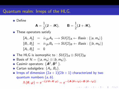
Quantum realm: Irreps of the HLG.
Define
A =1
2(J− iK), B =
1
2(J + iK),
These operators satisfy
[Ai ,Aj ] = iεijkAk −→ SU(2)A ← Basis : |a,ma〉[Bi ,Bj ] = iεijkBk −→ SU(2)B ← Basis : |b,mb〉[Ai ,Bj ] = 0
The HLG is isomorphic to : SU(2)A ⊗ SU(2)BBasis of H = |a,ma〉 ⊗ |b,mb〉.Casimir operators: A2,B2 .Cartan subalgebra: Az ,Bz.Irreps of dimension (2a + 1)(2b + 1) characterized by twoquantum numbers (a, b).
Λ (θ,ϕ) = e−i(J·θ+K ·ϕ) = e−i(A·(θ+iϕ)+B·(θ−iϕ))
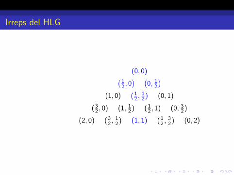
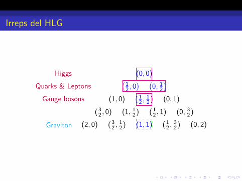
Irreps del HLG
(0, 0)(12 , 0) (
0, 12
)(1, 0) ( 1
2 ,12 ) (0, 1)
( 32 , 0) (1, 1
2 ) ( 12 , 1) (0, 3
2 )
(2, 0) ( 32 ,
12 ) (1, 1) ( 1
2 ,32 ) (0, 2)
Higgs
Quarks & Leptons
Gauge bosons
Graviton
Irreps del HLG
(0, 0)(12 , 0) (
0, 12
)(1, 0) ( 1
2 ,12 ) (0, 1)
( 32 , 0) (1, 1
2 ) ( 12 , 1) (0, 3
2 )
(2, 0) ( 32 ,
12 ) (1, 1) ( 1
2 ,32 ) (0, 2)
Higgs
Quarks & Leptons
Gauge bosons
Graviton

Chiral representations: (a, 0) y (0, b)
If a = 0: (0, b) representation
A = 0 ⇒ J = iK
⇒ B =1
2(J + iK) = J
(0, b) = (0, j) ≡ Left representation
ΛL (θ,ϕ) = e−iJ·(θ−iϕ)
If b = 0: (a, 0) representation
B = 0 ⇒ J = −iK
⇒ A =1
2(J− iK) = J
(a, 0) = (j , 0) ≡ Right representation
ΛR (θ,ϕ) = e−iJ·(θ+iϕ)
Chiral representations transform identically under rotationsbut have opposite transformation properties under boosts.
There are two representations with j = 12 .
We cannot distinguish them in the non-relativistic limit.How is the electron in our atoms connected to these irreps?
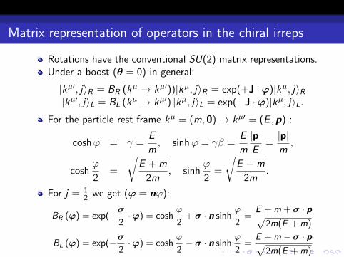
Matrix representation of operators in the chiral irreps
Rotations have the conventional SU(2) matrix representations.Under a boost (θ = 0) in general:
|kµ′, j〉R = BR (kµ → kµ′))|kµ, j〉R = exp(+J ·ϕ)|kµ, j〉R|kµ′, j〉L = BL (kµ → kµ′) |kµ, j〉L = exp(−J ·ϕ)|kµ, j〉L.
For the particle rest frame kµ = (m, 0)→ kµ′ = (E ,p) :
coshϕ = γ =E
m, sinhϕ = γβ =
E
m
|p|E
=|p|m,
coshϕ
2=
√E + m
2m, sinh
ϕ
2=
√E −m
2m.
For j = 12 we get (ϕ = nϕ):
BR (ϕ) = exp(+σ
2·ϕ) = cosh
ϕ
2+ σ · n sinh
ϕ
2=
E + m + σ · p√2m(E + m)
BL (ϕ) = exp(−σ2·ϕ) = cosh
ϕ
2− σ · n sinh
ϕ
2=
E + m − σ · p√2m(E + m)
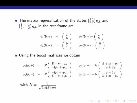
The matrix representation of the states |1212〉R,L and
|12 ,−12〉R,L in the rest frame are
φL(0,+) =
(10
)φR(0,+)=
(10
)φL(0,−) =
(01
)φR(0,−) =
(01
)
Using the boost matrices we obtain
φL(p,+) = N
(E + m − pz−(px + ipy )
)φR(p,+) = N
(E + m + pzpx + ipy
)φL(p,−) = N
(−(px − ipy )E + m + pz
)φR(p,−) = N
(px − ipy
E + m − pz
)
with N = 1√2m(E+m)
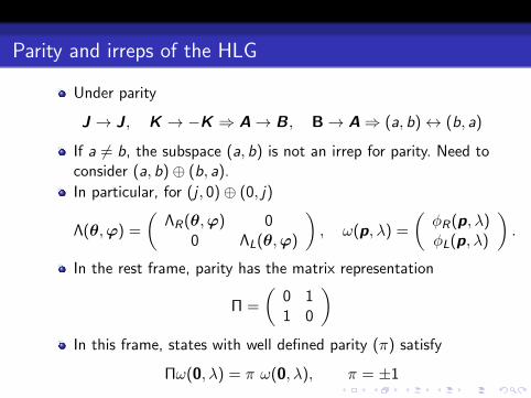
Parity and irreps of the HLG
Under parity
J → J , K → −K ⇒ A→ B, B→ A⇒ (a, b)↔ (b, a)
If a 6= b, the subspace (a, b) is not an irrep for parity. Need toconsider (a, b)⊕ (b, a).
In particular, for (j , 0)⊕ (0, j)
Λ(θ,ϕ) =
(ΛR(θ,ϕ) 0
0 ΛL(θ,ϕ)
), ω(p, λ) =
(φR(p, λ)φL(p, λ)
).
In the rest frame, parity has the matrix representation
Π =
(0 11 0
)In this frame, states with well defined parity (π) satisfy
Πω(0, λ) = π ω(0, λ), π = ±1
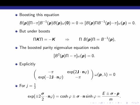
Boosting this equation
B(p)[Π−π]B−1(p)B(p)ω(0) = 0⇒ [B(p)ΠB−1(p)−π]ω(p) = 0.
But under boosts
ΠKΠ = −K ⇒ Π B(p)Π = B−1(p),
The boosted parity eigenvalue equation reads
[B2(p)Π− π]ω(p) = 0.
Explicitly(−π exp(2J · nϕ)
exp(−2J · nϕ) −π
)ω(p, λ) = 0
For j = 12
exp(±2σ
2· nϕ) = coshϕ± σ · n sinhϕ =
E ± σ · pm
.

For j = 12 the parity condition in an arbitrary frame reads(
−π E+σ·pm
E−σ·pm −π
)ω(p, λ) = 0.
Defining the following matrices
γ0 =
(0 11 0
), γi =
(0 −σiσi 0
)The parity condition reads
[γµpµ − πm]ω(p, λ, π) = 0.
Dirac equation is just the covariant form of parity eigenvalueequation in ( 1
2 , 0)⊕ (0, 12 ).
The γµ matrices satisfy
γµ, γν = 2gµν .
The explicit form of these matrices change if we change thechosen basis for ( 1
2 , 0)⊕ (0, 12 ).

Configuration space: Dirac Equation
Take positive parity π = 1 and define the configuration space”wave function”
ψ(x) = ω(p, λ, π)e−ip.x , i∂µψ(x) = pµψ(x).
It satisfies Dirac equation
[iγµ∂µ −m]ψ(x) = 0.
”Probability conservation” : ∂µJµ(r, t) = 0, with
Jµ(r, t) = ψγµψ, ψ ≡ ψ†γ0
”Probability density”
ρ(r, t) = ψγ0ψ = ψ†ψ

HLG irreps, quirality and elementary particles
j = 0: Higgs → (0, 0). Is not chiral.
j = 12 : quarks u, d , c , s, t, b and leptons e, µ, τ , νi ,
|f , λ〉 →|f , λ〉R → ( 1
2 , 0)|f , λ〉L → (0, 1
2 )
Electron in atoms has positive parity (convention)
|e−, λ〉 =1√2
(|e, λ〉R + |e, λ〉L).
The orthogonal state has the opposite parity: antiparticle.
|e+, λ〉 =1√2
(|e, λ〉R + |e, λ〉L).
j = 1: gauge bosons : γ, W+, W−,Z 0, gluon. transform inthe ( 1
2 ,12 ) irrep. Not chiral.
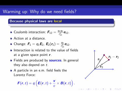
Warming up: Why do we need fields?
Because physical laws are local
Coulomb interaction: F12 = q1q2
r212
e12.
Action at a distance.
Change: F1 = q1E2, E2(r1) = q2
r212
e12.
Interaction is related to the value of fieldsat a given space point r .
Fields are produced by sources. In generalthey also depend on t.
A particle in an e.m. field feels theLorentz Force:
F (r , t) = q(E (r , t) +
vc× B(r , t)
).
r1
r2
r1 − r2
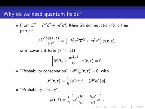
Why do we need quantum fields?
From E 2 = P2c2 + m2c4: Klein Gordon equation for a freeparticle
~2∂2φ(r, t)
∂t2=[−~2c2∇2 + m2c4
]φ(r , t),
or in covariant form (x0 = ct)[∂µ∂µ +
m2c2
~2
]φ(r, t) = 0,
”Probability conservation” : ∂µJµ(r, t) = 0, with
Jµ(r, t) =i
~[φ∗∂µφ− (∂µφ∗)φ] .
”Probability density”
ρ(r, t) =i
~
[φ∗∂φ
∂t− ∂φ∗
∂tφ
].

Free particle solutions : φ(x) = Ne−i~p·x yield
E = ±√
p2c2 + m2c4 ⇒ ρ = |N|22E
Negative energy solutions and negative probabilities. Noway.
Coupling to an electromagnetic field Aµ: Lorentz force ⇒”minimal coupling” : Pµ → Pµ − q
cAµ
[(∂µ + i
q
~cAµ)(∂µ + i
q
~cAµ) +
m2c2
~2
]φ(r, t) = 0.
Complex conjugated equation[(∂µ − i
q
~cAµ)(∂µ − i
q
~cAµ) +
m2c2
~2
]φ∗(r, t) = 0.

Notice:
If φ is a solution for a particle of charge q and mass m thenφ∗ is a solution for a particle of charge −q and same mass (”anti-particle” ).
These solutions cannot be equal (describe particles with theopposite charge). Both are solutions of the free KG equationwith mass m.
Conclusion: KG equation describes multiparticle states, atleast a pair of particles with same mass and opposite charge.
Single particle relativistic quantum mechanics is not tenable.
Multiparticle RQM= Quantum Fields
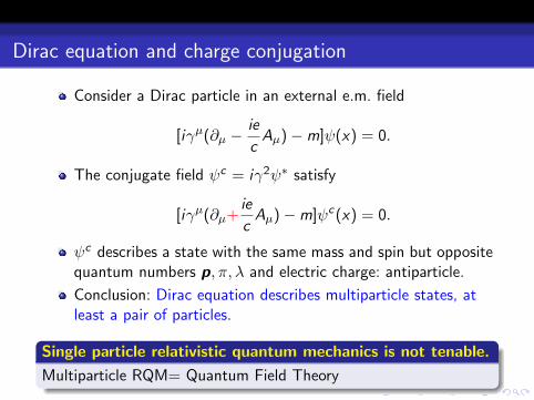
Dirac equation and charge conjugation
Consider a Dirac particle in an external e.m. field
[iγµ(∂µ −ie
cAµ)−m]ψ(x) = 0.
The conjugate field ψc = iγ2ψ∗ satisfy
[iγµ(∂µ+ie
cAµ)−m]ψc(x) = 0.
ψc describes a state with the same mass and spin but oppositequantum numbers p, π, λ and electric charge: antiparticle.
Conclusion: Dirac equation describes multiparticle states, atleast a pair of particles.
Single particle relativistic quantum mechanics is not tenable.
Multiparticle RQM= Quantum Field Theory

Natural units
Fundamental constants and units:
[~] = Et, [c] = L/t, [~c] = EL, [mc2] = E , [kBT ] = E
Time, lenght, mass and temperature
[~E
] = t, [~cE
] = L, [E
c2] = m, [
E
kB] = T
Fundamental constants apart we get
t = [1
E], L = [
1
E], m = [E ], T = [E ]
Basic conversion factors:
1seg = 1,5× 1024GeV−1~1m = 5× 10¹⁵GeV−1~c
1Kg = 5,62× 1026GeV /c2
H0 = 1,53× 10−42GeV /~GF = 1,16× 10⁻⁵GeV−2(~c)3
MP = 1,22× 10¹⁹GeV /c2
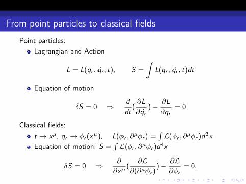
From point particles to classical fields
Point particles:
Lagrangian and Action
L = L(qr , qr , t), S =
∫L(qr , qr , t)dt
Equation of motion
δS = 0 ⇒ d
dt(∂L
∂qr)− ∂L
∂qr= 0
Classical fields:
t → xµ, qr → φr (xµ), L(φr , ∂µφr ) =
∫L(φr , ∂
µφr )d3x
Equation of motion: S =∫L(φr , ∂
µφr )d4x
δS = 0 ⇒ ∂
∂xµ(
∂L∂(∂µφr )
)− ∂L∂φr
= 0.

Klein-Gordon Lagrangian: complex scalar field
L = ∂µφ∗∂µφ−m2φ∗φ+Ω
∂L∂(∂µφ∗)
= ∂µφ,∂L∂φ∗
= −m2φ
∂L∂(∂µφ)
= ∂µφ∗,
∂L∂φ
= −m2φ∗
Euler-Lagrange equations for φ∗ and φ yield
(∂µ∂µ + m2)φ = 0
(∂µ∂µ + m2)φ∗ = 0

Conserved currents
Noether’s theorem
Every continuous symmetry of the action yields a conservedcurrent ∂µJµ = 0.
Consider the transformation of the fields: δφr ≡ Xr (φ). If δS = 0then the Lagrangian density can change at most by a totaldivergence δL = ∂µFµ(φ). But
δL =∂L∂φr
δφr +∂L
∂(∂µφr )δ(∂µφr )
= (∂L∂φr− ∂µ ∂L
∂(∂µφr ))δφr + ∂µ(
∂L∂(∂µφr )
δφr ).
Thus
∂µ(
∂L∂(∂µφr )
Xr (φ)− Fµ(φ)
)= 0.
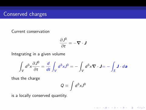
Conserved charges
Current conservation
∂J0
∂t= −∇ · J
Integrating in a given volume∫Vd3x
∂J0
∂t=
d
dt
∫Vd3xJ0 = −
∫Vd3x∇ · J= −
∫SJ · da
thus the charge
Q ≡∫
d3xJ0
is a locally conserved quantity.

Space-time translations
Space-time translations: xµ → xµ + εµ
φr → φr + εµ∂µφr ⇒ δφr = εµ∂µφr = Xr .
L → L+ εµ∂µL ⇒ δL = ∂µ(εµL)⇒ Fµ = εµL.
Noether’s current
Jµ =∂L
∂(∂µφr )εα∂αφr − εµL
There is a conserved current for each value of εν
Tµν =
∂L∂(∂µφr )
∂νφr − gµνL, ∂µTµν = 0.
Conserved charges: energy and momentum
E =
∫d3xT 0
0 =
∫d3x(
∂L∂(∂0φr )
∂0φr − L),
Pi =
∫d3xT 0
i =
∫d3x
∂L∂(∂0φr )
∂iφr .

For the KG field
L = ∂µφ∗∂µφ−m2φ∗φ+Ω
E =
∫d3x [∂0φ∗∂0φ+∇φ∗ ·∇φ+ m2φ∗φ−Ω],
Pi =
∫d3x [∂0φ∗∂iφ+ ∂iφ
∗∂0φ].
Internal symmetries:U(1)
The KG Lagrangian is invariant under global U(1) transformations
φ→ φ′ = U(θ)φ ≡ e−iqθφ ⇒ δφ = −iqθφ, δφ∗ = iqθφ∗
The Noether current is
Jµ = iq(∂L
∂(∂µφ∗)φ∗ − ∂L
∂(∂µφ)φ)
= iq(φ∗∂µφ− (∂µφ∗)φ)
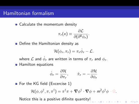
Hamiltonian formalism
Calculate the momentum density
πr (x) ≡ ∂L∂(∂0φr )
.
Define the Hamiltonian density as
H(φr , πr ) = πr φr − L.
where L and φr are written in terms of πr and φr .
Hamilton equations
φr =∂H∂πr
, πr = − ∂H∂φr
For the KG field (Excercise 1)
H(φ, φ†, π, π†) = π†π +∇φ† ·∇φ+ m2φ†φ−Ω.
Notice this is a positive difinite quantity!
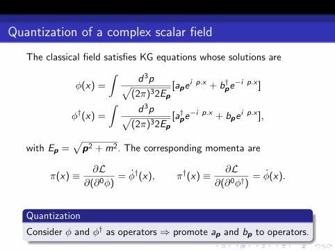
Quantization of a complex scalar field
The classical field satisfies KG equations whose solutions are
φ(x) =
∫d3p√
(2π)32Ep[ape
i p.x + b†pe−i p.x ]
φ†(x) =
∫d3p√
(2π)32Ep[a†pe
−i p.x + bpei p.x ],
with Ep =√
p2 + m2. The corresponding momenta are
π(x) ≡ ∂L∂(∂0φ)
= φ†(x), π†(x) ≡ ∂L∂(∂0φ†)
= φ(x).
Quantization
Consider φ and φ† as operators ⇒ promote ap and bp to operators.

In NRQM, the Heisenberg picture operators Xi (t), Pj(t) satisfy
[Xi (t),Pj(t)] = i~δij , [Xi (t),Xj(t)] = 0, [Pi (t),Pj(t)] = 0.
Field quantization is realized imposing the equal time commutationrelations
[φi (x , t), πj(y , t)] = iδijδ(x − y),
[φi (x , t), φj(y , t)] = 0, [πi (x , t), πj(y , t)] = 0.
These commutators require
[ap, a†q ]= δ3(p − q), [ap, aq ] = 0, [a†p, a
†q ] = 0,
[bp, b†q ]= δ3(p − q), [bp, bq ] = 0, [b†p, b
†q ] = 0,
[ap, bq ] = 0, [ap, b†q ] = 0, [a†p, bq ] = 0, [a†p, b
†q ] = 0.
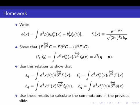
Homework
Write
φ(x) =
∫d3p[apf
∗p (x) + b†pfp(x)], fp(x) ≡ e−i p.x√
(2π)32Ep
Show that (F←→∂0G ≡ F∂0G − (∂0F )G )
〈fp|fq〉 ≡∫
d3xf ∗p (x)i←→∂0 fq(x) = δ3(q − p).
Use this relation to show that
aq =
∫d3xφ(x)i
←→∂0 fq(x), a†q =
∫d3xf ∗q (x)i
←→∂0φ†(x)
bq =
∫d3xφ†(x)i
←→∂0 fq(x), b†q =
∫d3xf ∗q (x)i
←→∂0φ(x)
Use these results to calculate the commutators in the previousslide.

Noether’s charges
A straightforward calculation yields
H ≡∫
[φ†φ+∇φ† ·∇φ+ m2φ†φ−Ω]d3x
=
∫d3p Ep
(a†pap +
1
2δ3(0) + b†pbp +
1
2δ3(0)
)−ΩV
P =
∫d3x [φ†∇φ+ (∇φ†)φ]
=
∫d3p p
(a†pap+
1
2+ b†pbp+
1
2
),
Q = q
∫d3xφ†i
←→∂0φ = q
∫d3p
(a†pap − b†pbp
),
These operators commute with each other
[H,P] = 0, [H,Q] = 0, [Q,P] = 0.

Defining Nap ≡ a†pap and Nb
p = b†pbp we get
[Nap ,N
bq ] = 0, [Na
p ,Naq ] = 0, [Nb
p ,Nbq ] = 0
[Nap , a†q ] = a†pδ
3(p − q), [Nap , aq ] = −apδ
3(p − q),
[Nbp , b†q ] = b†pδ
3(p − q), [Nbp , bq ] = −bpδ
3(p − q).
Define now the total N operators
Na =
∫d3p a†pap, Nb =
∫d3p b†pbp.
Notice that Q = q(Na − Nb). These operators satisfy
[Na,Nb] = 0, [Na,b,H] = 0, [Na,b,P] = 0, [Na,b,Q] = 0.
The operators H,P,Q,Na,Nb form a complete set ofcommuting operators
Quantum states are labelled by their eigenvalues (good quantumnumbers): |E ,p, q(na − nb), na, nb〉.
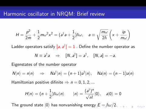
Harmonic oscillator in NRQM: Brief review
H =p2
2m+
1
2mω2x2 = (a†a +
1
2)~ω, a ≡
√mω
2~
(x +
ip
mω
)Ladder operators satisfy [a, a†] = 1 . Define the number operator as
N ≡ a†a ⇒ [N, a†] = a†, [N, a] = −a.
Eigenstates of the number operator
N|n〉 = n|n〉 ⇒ Na†|n〉 = (n + 1)a†|n〉, Na|n〉 = (n − 1)a|n〉
Hamiltonian positive difinite ⇒ n = 0, 1, 2, ...
H|n〉 = (n +1
2)~ω|n〉 |n〉 =
(a†)n√n!|0〉, a|0〉 = 0
The ground state |0〉 has nonvanishing energy E = ~ω/2.

Interpretation
The KG field consists of a collection of HO’s, two (a or b) foreach value of p.The ground state of the p-HO satisfy
Nap |0p〉a = 0, Nb
p |0p〉b = 0.
Denote the collective ground state by |0〉 = Π⊗p |0p〉For the ground state we get
Na|0〉 =
∫d3p Na
p|0〉= 0, Nb|0〉 =
∫d3p Nb
p |0〉= 0
H|0〉 =
[∫d3p Ep(Na
p + Nbp + δ3(0))− ΩV
]|0〉≡ (E0 − Ω)V |0〉,
P|0〉 =
∫d3p p(Na
p + Nbp )|0〉= 0,
Q|0〉 = q
∫d3p(Na
p − Nbp )|0〉= 0.

Energy of the ground state
The zero-point energy of the harmonic oscillators yield∫d3p Epδ
3(0) =
∫d3p Ep
∫d3x
(2π)3e iq.x |q=0 =
V
(2π)3
∫d3p Ep
This is formally an infinite amount of energy.
However, we have learnt that our theories are valid only up tosome energy (effective theories).
We expect QFT description to be appropriate up to someenergy scale Λ m. The corresponding energy density is
E0 =
∫d3p
(2π)3Ep =
4π
(2π)3
∫ Λ
m
√E 2 −m2E 2dE =
Λ4
8π2.
Choose Ω = E0
H =
∫d3p Ep(Na
p + Nbp ), H|0〉 = 0.
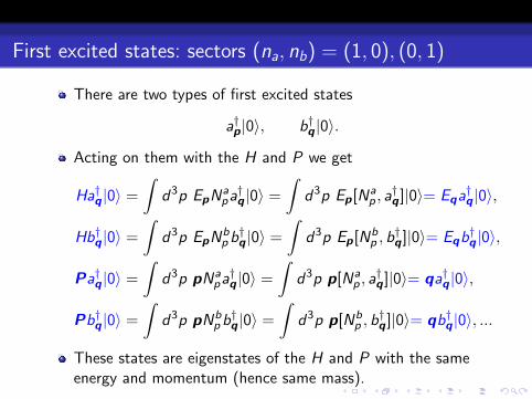
First excited states: sectors (na, nb) = (1, 0), (0, 1)
There are two types of first excited states
a†p|0〉, b†q |0〉.
Acting on them with the H and P we get
Ha†q |0〉 =
∫d3p EpN
apa†q |0〉 =
∫d3p Ep[Na
p , a†q ]|0〉= Eqa
†q |0〉,
Hb†q |0〉 =
∫d3p EpN
bpb†q |0〉 =
∫d3p Ep[Nb
p , b†q ]|0〉= Eqb
†q |0〉,
Pa†q |0〉 =
∫d3p pNa
pa†q |0〉 =
∫d3p p[Na
p , a†q ]|0〉= qa†q |0〉,
Pb†q |0〉 =
∫d3p pNb
pb†q |0〉 =
∫d3p p[Nb
p , b†q ]|0〉= qb†q |0〉, ...
These states are eigenstates of the H and P with the sameenergy and momentum (hence same mass).

But they have opposite U(1) charge eigenvalues...
Qa†q |0〉 = q
∫d3pNa
pa†q |0〉 = q
∫d3p [Na
p , a†q ]|0〉= qa†q |0〉,
Qb†q |0〉 = −q∫
d3pNbpb†q |0〉 = −q
∫d3p [Nb
p , b†q ]|0〉= −qb†q |0〉.
...and different Na,Nb eigenvalues
Naa†q |0〉 =
∫d3pNa
pa†q |0〉 =
∫d3p [Na
p , a†q ]|0〉= a†q |0〉,
Nab†q |0〉= 0, Nba†q |0〉 = 0,
Nbb†q |0〉 =
∫d3pNb
pb†q |0〉 =
∫d3p [Nb
p , b†q ]|0〉= b†q |0〉.
Finally
a†p|0〉 = |E ,p, q, 1, 0〉 ≡ |p〉a, b†p|0〉 = |E ,p,−q, 0, 1〉 ≡ |p〉b
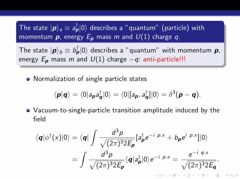
The state |p〉a ≡ a†p|0〉 describes a ”quantum” (particle) withmomentum p, energy Ep mass m and U(1) charge q.
The state |p〉b ≡ b†p|0〉 describes a ”quantum” with momentum p,energy Ep mass m and U(1) charge −q: anti-particle!!!
Normalization of single particle states
〈p|q〉 = 〈0|apa†q |0〉 = 〈0|[ap, a
†q ]|0〉 = δ3(p − q).
Vacuum-to-single-particle transition amplitude induced by thefield
〈q|φ†(x)|0〉 = 〈q|∫
d3p√(2π)32Ep
[a†pe−i p.x + bpe
i p.x ]|0〉
=
∫d3p√
(2π)32Ep〈q|a†p|0〉e−i p.x =
e−i q.x√(2π)32Eq
.
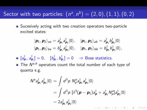
Sector with two particles: (na, nb) = (2, 0), (1, 1), (0, 2)
Sucesively acting with two creation operators two-particleexcited states:
|p1,p2〉aa = a†p1a†p2|0〉, |p1,p2〉ab = a†p1
b†p2|0〉
|p1,p2〉ba = b†p1a†p2|0〉, |p1,p2〉bb = b†p1
b†p2|0〉,
[a†pi , a†pj ] = 0, [b†pi , b
†pj ] = 0 ⇒ Bose statistics.
The Na,b operators count the total number of each type ofquanta e.g.
Naa†p1a†p2|0〉 =
∫d3p Na
pa†p1a†p2|0〉
=
∫d3p [δ3(p − p1)a†p + a†p1
Nap ]a†p2
|0〉
= 2a†p1a†p2|0〉
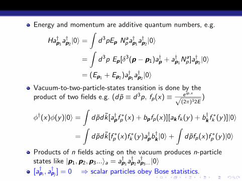
Energy and momentum are additive quantum numbers, e.g.
Ha†p1a†p2|0〉 =
∫d3pEp Na
pa†p1a†p2|0〉
=
∫d3p Ep[δ3(p − p1)a†p + a†p1
Nap ]a†p2
|0〉
= (Ep1 + Ep2)a†p1a†p2|0〉
Vacuum-to-two-particle-states transition is done by theproduct of two fields e.g. (dp ≡ d3p, fp(x) ≡ e ip.x√
(2π)32E)
φ†(x)φ(y)|0〉 =
∫dpdk[a†pf
∗p (x) + bpfp(x)][ak fk(y) + b†k f
∗k (y)]|0〉
=
∫dpdk[f ∗p (x)f ∗k (y)a†pb
†k |0〉+
∫dpfp(x)f ∗p (y)|0〉
Products of n fields acting on the vacuum produces n-particlestates like |p1,p2,p3...〉a = a†p1a
†p2a†p3...|0〉
[a†pi , a†pj ] = 0 ⇒ scalar particles obey Bose statistics.
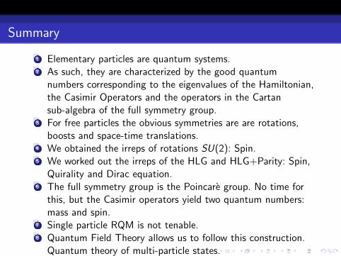
Summary
1 Elementary particles are quantum systems.2 As such, they are characterized by the good quantum
numbers corresponding to the eigenvalues of the Hamiltonian,the Casimir Operators and the operators in the Cartansub-algebra of the full symmetry group.
3 For free particles the obvious symmetries are are rotations,boosts and space-time translations.
4 We obtained the irreps of rotations SU(2): Spin.5 We worked out the irreps of the HLG and HLG+Parity: Spin,
Quirality and Dirac equation.6 The full symmetry group is the Poincare group. No time for
this, but the Casimir operators yield two quantum numbers:mass and spin.
7 Single particle RQM is not tenable.8 Quantum Field Theory allows us to follow this construction.
Quantum theory of multi-particle states.


![Classical Mechanics - people.phys.ethz.chdelducav/cmscript.pdf · References [1]LandauandLifshitz,Mechanics,CourseofTheoreticalPhysicsVol.1., PergamonPress [2]Classical Mechanics,](https://static.fdocuments.us/doc/165x107/5e1e9832bac1ea74484e9601/classical-mechanics-delducavcmscriptpdf-references-1landauandlifshitzmechanicscourseoftheoreticalphysicsvol1.jpg)