Introduction to the Real Numbers - Colorado State …calc/M517/vol1.pdfIntroduction to the Real ......
245
Chapter 1 Introduction to the Real Numbers 1.1 Introduction Most students feel that they have an understanding of the real numbers and/or the real line. Throughout most of your education you have drawn a line— sometimes called a number line—having a positive (and hence negative) di- rection and with the integers indicated. From this you could approximately designate any other real number. You used two of these as axes when you graphed functions. When you learned how to take limits as x → a, you used a number line as the x-axis when you (or the instructor or the book) explained the meaning of the concept of a limit. When you were introduced to integrals, an interval on the real line was subdivided to aid in the definition of the integral. Unless you were given an non-standard introduction to these concepts you really didn’t know enough about the real line to know what’s missing. You surely don’t know enough about the real line to be able prove the important calculus theorems. This isn’t as bad as it may sound. When Isaac Newton and Gottfried Wil- helm Leibniz invented calculus in the late 1600’s, they used a very intuitive approach. After a while some people started pointing out that there were in- consistencies to their approaches. Over the next 200 years many of the great mathematicians worked on rigorizing calculus. In 1754 Jean-le-Rond d’Alembert decided that it was necessary to give a rigorous treatment of limits. Joseph Louis Lagrange published his first paper rigorizing calculus in 1797. As a part of his work on hypergeometric series, in 1812 Carl Freidrich Gauss gave rigorous dis- cussion of the convergence of an infinite series. And finally, Augustus-Louis Cauchy in 1821 answered d’Alembert’s call and introduced a theory of lim- its. In 1874 Karl Weierstrass gave an example of an everywhere continuous, nowhere differentiable function. This example illustrated that geometric intu- 1
Transcript of Introduction to the Real Numbers - Colorado State …calc/M517/vol1.pdfIntroduction to the Real ......

Chapter 1
Introduction to the Real
Numbers
1.1 Introduction
Most students feel that they have an understanding of the real numbers and/orthe real line. Throughout most of your education you have drawn a line—sometimes called a number line—having a positive (and hence negative) di-rection and with the integers indicated. From this you could approximatelydesignate any other real number.
You used two of these as axes when you graphed functions. When youlearned how to take limits as x→ a, you used a number line as the x-axis whenyou (or the instructor or the book) explained the meaning of the concept of alimit. When you were introduced to integrals, an interval on the real line wassubdivided to aid in the definition of the integral.
Unless you were given an non-standard introduction to these concepts youreally didn’t know enough about the real line to know what’s missing. Yousurely don’t know enough about the real line to be able prove the importantcalculus theorems.
This isn’t as bad as it may sound. When Isaac Newton and Gottfried Wil-helm Leibniz invented calculus in the late 1600’s, they used a very intuitiveapproach. After a while some people started pointing out that there were in-consistencies to their approaches. Over the next 200 years many of the greatmathematicians worked on rigorizing calculus. In 1754 Jean-le-Rond d’Alembertdecided that it was necessary to give a rigorous treatment of limits. Joseph LouisLagrange published his first paper rigorizing calculus in 1797. As a part of hiswork on hypergeometric series, in 1812 Carl Freidrich Gauss gave rigorous dis-cussion of the convergence of an infinite series. And finally, Augustus-LouisCauchy in 1821 answered d’Alembert’s call and introduced a theory of lim-its. In 1874 Karl Weierstrass gave an example of an everywhere continuous,nowhere differentiable function. This example illustrated that geometric intu-
1

2 1. Real Numbers
ition was not an adequate tool for analytic studies. Weierstrass realized thatto perform rigorous analysis there must be an understanding of the real num-ber system. Weierstrass instigated a program known as the arithmetization ofanalysis which through the work of Weierstrass and his followers establishedthe rigorous treatment of the real number system as a foundation for classicalanalysis. Weierstrass died in 1897.
Summarizing the situation, it took them 200 years from when they were firstintroduced to the ideas of calculus until they arrived at an understanding of howand why calculus really works. So it’s not too bad that you may have startedlearning calculus two or three years ago and some of the important essentialswere skipped.
This chapter serves as an introduction to the set of real numbers. There areat least three common approaches of introducing the set of real numbers. Formany people the approaches using either Dedekin cuts (where the real numbersare represented by sets of rational numbers) or Cauchy sequences (where the realnumbers are represented by equivalence classes of Cauchy sequences of rationalnumbers) are more satisfying in that you actually construct the set of reals.In either case, however, neither the rationals nor the reals look like numbersthat you are accustomed to using. Instead of using either of these approacheswe shall describe the set of real numbers by a suitable set of postulates. Oneadvantage of this approach is that it is the fastest (and we don’t want to spendtoo much time on it). In addition, the set of postulates give us a very explicitlist of the most basic properties satisfied by real numbers.
In addition to introducing the real numbers in this chapter, we will discusscertain aspects of proofs. We feel that this necessary or at least advantageousto help the reader understand the proofs given in this text.
Before we get started we will review some things that we know (or at leastwe think we know), introduce some notation and discuss some useful results andideas. We begin by defining the sets
• the set of natural numbers N = {1, 2, 3, · · · },
• the set of integers Z = {· · · ,−3,−2,−1, 0, 1, 2, 3, · · ·},
• the set of rational numbers Q = {m/n : m,n ∈ Z, n 6= 0}.
Of course N ⊂ Z ⊂ Q. The description of Q is not ideal. It’s not wrongbut it doesn’t take care of the fact that there are multiple descriptions of eachrational number, i.e. 1/2 = 3/6 = 123/246, etc. One complicated way aroundthis is to define a rational number as the equivalence class of rational numbersthat are equal. It’s a bit easier to just always consider the rational numberin ”reduced form” where common multiples of the integers in the numeratorand the denominator have been divided out. We will take this latter approach.Hence the ”rational numbers” 1/2, 3/6 and 123/246 are all represented by 1/2.
One way to introduce the need for the real number system is to start with theset of rational numbers and decide that something important is missing. If yougraph the function f(x) = 2−x2 really carefully using only the rational numbers

1.1 Introduction 3
on the x-axis, you see that the graph passes through the x-axis without hittingthe axis—we don’t want that but then you really can’t graph it that carefully.
Many of you have seen the common proof that√
2 is not rational whichgoes as follows. (Read the proof carefully. It’s not terribly important to beable to reproduce the proof but it is important that you can follow the proof.)Assume false, i.e. that
√2 is rational. Then
√2 = m/n where m and n are in
Q, n 6= 0 and m/n is in reduced form. If we square both sides we get m2 = 2n2.Since m2 is a multiple of 2, m2 is even. This implies that m is even. (If mis not even, i.e. m is odd, then m = 2k + 1 for some integer k. But thenm2 = (2k+1)2 = 4k2 +4k+1 = 2(2k2 +2k)+1 is odd. This is a contradiction.)If m is even, then m can be written as m = 2k. But then the facts that m = 2kand m2 = 2n2 imply that m2 = 4k2 = 2n2 or n2 = 2k2. Thus n must alsobe even. This is a contradiction to the fact that we assumed that m/n was inreduced form.
Thus we see that√
2 is not rational. But do we really care? Do we needa√
2 in our lives? With a little bit of thought about the diagonal of the unitsquare or the graph of the functions f(x) = 2−x2, it’s reasonably clear that wewant to have
√2 in our number system, i.e. Q is not enough. In general, we do
not want to work on domains that have holes in them like Q has at√
2.It should be pretty clear that there are a lot of rational numbers (there are
a lot of natural numbers and there are clearly a lot more rational numbers thanthere are natural numbers). A little thought will at convince you that there arealso a lot of numbers on the number line that are not rational. A proof similarto the one given above will show that
√3 and
√7 are not rational. It’s also easy
to prove that q√
2 (Example 1.2.2) and q +√
2 (HW1.2.2–(a)) are not rationalfor any q ∈ Q. Since there are a lot of what we think of as numbers that arenot rational, there are many holes in Q.
What we would like to do is to figure out how to fill in the holes in the realnumber line of the numbers that are not rational. This is close to what theapproaches to building the real numbers using either Dedekin cuts or Cauchysequences do. We will really approach this from the other direction. We willdefine the set of real numbers and then show that this set is what we want.
Before we go on, we would like to include a topic related to our work withthe rational numbers. The following result makes it easy to show that a givennumber is not rational—and it shows more. Consider the following proposition.
Proposition 1.1.1 Consider the polynomial equation
a0xn + a1x
n−1 + · · · + an−1x+ an = 0 (1.1.1)
where a0, a1, · · · , an are integers, a0 6= 0, an 6= 0 and n ≥ 1. Let r ∈ Q be a rootof equation (1.1.1) where r = p/q expressed in reduced form. Then q divides a0
and p divides an.
Proof: If you observe carefully, you will see that the proof of this propositionis really very similar to the way that we proved that
√2 was not rational.

4 1. Real Numbers
If r = p/q is a root of equation (1.1.1), then a0
(
p
q
)n
+ a1
(
p
q
)n−1
+ · · · +
an−1
(
p
q
)
+ an = 0. Multiplying by qn we get
a0pn + a1p
n−1q + · · · + an−1pqn−1 + anq
n = 0. (1.1.2)
Solving for a0pn allows us to rewrite equation (1.1.2) as
a0pn = −q
[
a1pn−1 + a2p
n−3q + · · · + anqn−1]
.
Since everything inside of the brackets is an integer, q must divide a0pn. Since
p/q is in reduced form, no factors of q divide out with any part of pn (seeHW1.1.1). Thus, q divides a0.
Likewise, we rewrite equation (1.1.2) as
anqn = −p
[
a0pn−1 + a1p
n−2q + · · · + an−1qn−1]
.
We use the same argument as before. Because p must divide anqn and no factors
of p can divide out any factors of qn, then p must divide an.
Before we show you how nice this result is in relation to our work withrational numbers, let us remind you that you have probably used this resultbefore. A while after you learned how to factor polynomials in your algebraclasses, you were faced with factoring polynomials of degree greater than orequal to three. You were given a problem like ”factor 2x3 + 3x2 − 8x+ 3.” Youwere taught to try to divide by x±3, x±3/2, x±1/2 and x±1. These potentialroots were formed by trying all rationals p/q where p is a factor of an = 3 andq is a factor of a0 = 2, i.e. by applying Proposition 1.1.1. If and when you werelucky enough to divide 2x3 + 3x2 − 8x+ 3 by x− 1 you got
2x3 + 3x2 − 8x+ 3
x− 1= 2x2 + 5x− 3.
You then factored the quadratic term which gives you the complete factorization
2x3 + 3x2 − 8x+ 3 = (x− 1)(2x− 1)(x+ 3).
If none of the potential roots satisfy the equation, Proposition 1.1.1 impliesthat there are no rational roots. In you algebra class you usually didn’t have toworry about that since they were trying to teach you how to factor—one of thepotential roots always satisfied the equation.
Our application of Proposition 1.1.1 goes as follows. Consider the equationx2 − 2 = 0. By Proposition 1.1.1 we know that if there are going to be rationalroots to this equation, they will be either ±2 or ±1. It is easy to try thesefour potential roots and see that none of them satisfy the equation x2 − 2 =0. Therefore the equation has no rational roots. Solving for x we know thatx = ±
√2 represents the solutions to this equation. Therefore ±
√2 must not be
rational.

1.2 Proofs 5
This same approach can be used to produce many numbers that are notrational. Many such as
√13 are as easy as
√2. For some it is more difficult
to find the appropriate algebraic equation associated with the number but the
method still works. For example consider the number3
√
4−√
23 . Set x =
3
√
4−√
23 .
Then x3 = 4−√
23 , 3x3 = 4 −
√2, 3x3 − 4 = −
√2 and
(
3x3 − 4)2
= 2. Expandthis last expression and apply Proposition 1.1.1 to the resulting polynomial
(with integer coefficients). Surely 3
√
4−√
23 is a root of this polynomial.
HW 1.1.1 Assume that p and q have the prime factorizations p1 · · · pmp andq1 · · · qmq , respectively and p/q is in reduced form. Prove that if q divides a0p
n
(where a0 is an integer), then q divides a0.
HW 1.1.2 Prove that√
13 is not rational.
HW 1.1.3 Prove that 32 +
√13 is not rational.
1.2 Introduction to Proofs
Before we proceed with the next step of defining the set of real numbers, wepause to include a short discussion of proofs. This topic is surely a bit of adetour but it may prove to be helpful. In a text such as this, proofs are veryimportant. It is a time in your mathematical career when you see why thingsare true. It is a time when you learn to write a proof that convinces the readerthat what you claim is indeed true. Probably most importantly, you learn toread mathematics (specifically mathematical proofs) critically and be able toevaluate whether the writers argument is sound and if what the writer claimsis true is in fact true.
Two types of proofs are important in mathematics: the direct proof and theindirect proof. We will first discuss the simplest case, direct proof.
Direct Proofs: A direct proof is a valid argument with true premises. Inour cases the true premises are usually axioms and definitions that have beengiven, or previously proved results. If the statement to be proved is in theform p implies q (which our statements will often be), then we can include thestatement p as one of the true premises. A valid argument should be defined andstudied in a logic class—but not many logic classes exist anymore. We will tryto show you what a valid argument is through a series of examples—just aboutall (hopefully all) of the proofs in this text give examples of valid proofs. Thevalid argument is a series of logical implications relating know facts resulting inthe desired conclusion. Consider the following example.
Example 1.2.1 Prove that r1, r2 ∈ Q implies r1 + r2 ∈ Q.
Solution: The list of known facts mentioned as a part of the proof includesthe statement r1, r2 ∈ Q, the definition of Q and all known properties ofarithmetic for rational numbers. (We know more. That means that there are

6 1. Real Numbers
more potential hypotheses but these would not tend to be relevant here.) Theargument to prove this statement can be given as follows:
r1, r2 ∈ Q implies that r1 = m1/n1 and r2 = m2/n2 for m1,m2, n1, n2 ∈ Z
(by the definition of Q). Then r1 + r2 =m1
n1+m2
n2=m1n2 + n1m2
n1n2(by know
arithmetic for integers). m1,m2, n1, n2 ∈ Z implies that m1n2+n1m2, n1n2 ∈ Z
(because Z is closed with respect to addition and multiplication). Thereforer1 + r2 is the ratio of two integers or r1 + r2 is rational (by the definition of Q).
This is a very easy proof but it is hoped that it shows explicitly what the”true hypotheses” are and how these hypotheses fit together with the validargument to construct the proof. We will have more difficult direct proofs, butmore difficult direct proofs will just be more difficult analogs to this proof. Weshould realize that the statement p implies q can also be written as if p, then q,p is a sufficient condition for q, p only if q and q is a necessary condition for p.Depending on the author you may see all of these different expressions.
And finally we discuss again what we mean by true premises. It is diffi-cult when you leave the ”do as I say” world of mathematics to the ”prove it”world of mathematics. At this time you ”know” a lot of things that have beentold to you—things that have not been based on a firm mathematical founda-tion. Students sometimes have trouble knowing what they can assume are truepremises. It is clear that you can assume anything that we have given you aspostulates, definitions or anything that you or we have proved. We did cheat abit when we have told you that you know about the integers, the arithmetic forintegers and consequently the arithmetic for rationals. Actually, the facts thatyou know for the integers include a small set of postulates and results provedfrom those postulates. Because we had to start somewhere, we assume that youknow those. When it is necessary, we will include some of the properties of theintegers—postulated and/or proved. Just about every other true premise thatyou will have to use or we will use will be included in this text. If we cheat, wewill try to remember to tell you that we are cheating.
Indirect Proofs: Indirect proofs are very common in analysis. There arecertain results that are very difficult to prove directly yet can be easily provedusing an indirect proof. The indirect proofs are based on the logical conceptsof the contrapositive and the contradiction. We discuss first the use of thecontrapositive in proof.
The Contrapositive: When the statement we wish to prove is if r, then s,a common approach to proving the statement is to consider the contrapositiveof the statement. For this short discussion we will write the implication asr → s and read it as p implies q. The contrapositive of the statement r → sis the statement (∼ s) → (∼ r) where (∼ s) mean ”not s”. We refer to ∼ sas the negation of s. An example of an implication that we proved earlier isn2 is even implies that n is even (where the context implied that n ∈ Z). Thecontrapositive of this statement is n is not even implies n2 is not even or n isodd implies n2 is odd. It is not clear or easy to see that the statements n2 is even

1.2 Proofs 7
r s r → s ∼ s ∼ r (∼ s) → (∼ r)
T T T F F TT F F T F FF T T F T TF F T T T T
Table 1.2.1: Truth table for the contrapositive.
implies that n is even and n is odd implies n2 is odd are equivalent. The easiestway is to construct a simple truth table including r → s and (∼ s) → (∼ r).
The first two columns of the Table 1.2.1 list all combinations of truth valuesof the statements r and s, both r and s can be true or false. Column 3 canbe thought of the definition of the truth value of the implication. The point isthat the implication is only bad (i.e. false) if a true hypothesis implies a falseconclusion (row 2). Otherwise the implication is true. Columns 4 and 5 give thetruth values of the statements ∼ s and ∼ r (opposite of those of s and r). Andfinally, column 6 gives the truth values of the statement (∼ s) → (∼ r) basedon the definition of the truth values of the implication (i.e. false only when atrue statement will imply a false statement) and the truth values of ∼ s and∼ r. We note that the truth values of r → s and (∼ s) → (∼ r) are the same.That means that the statements r → s and (∼ s) → (∼ r) are equivalent.
The result of the argument is to prove the statement r implies s is equivalentto proving the statement not s implies not r, or using our example, to prove thestatement n2 is even implies n is even is equivalent to proving the statementn is odd implies n2 is odd. This is good because the latter statement is veryeasy to prove directly. The first statement is very difficult (if not impossible)to prove directly. This proof was given in the previous section as a part of theproof that
√2 is not rational (before you knew that you were doing a proof by
proving the contrapositive of a statement). Therefore we use the easy argumentto prove that n is odd implies n2 is odd. Then this will also imply that n2 iseven implies n is even.
Contradiction The second type of indirect proof is based on the logicalconcept of a contradiction. A contradiction is a statement that is false for allcombinations of the truth values. A proof by contradiction, or when you arereally pleased with your proof you might refer to it as a proof by reductio adabsurdum, is based on the fact that if p1 is a statement, then it is impossible forp1 and ∼ p1 to both be true. Recall that a proof is a valid argument with truepremises. If we lump everything that we know to be true (including anythingthat we can prove based on what we know to be true) into one statement calledpK (where if the statement we wish to prove looks like r → s, we also includethe r in pK), a proof is of the form pK → q where q is true whenever pK is true.
When we prove a statement s or r → s be contradiction, we begin by as-suming that the statement s is false. We then proceed to use this informationto prove that some statement p1 is false, where p1 is one of the statements in-

8 1. Real Numbers
cluded in pK or r, in the case that the statement that we want to prove is ofthe form r → s. In either case we will have assumed initially that p1 is trueand have proved that p1 is false, which is a contradiction both by Webster’sdefinition and by a mathematical definition—because then p1 ∧ (∼ p1) is surelyalways false. Thus our original assumption that the statement s was false mustbe erroneous—thus the statement s must be true.
In Section 1.1 we proved that the√
2 was not rational. We did it at thattime—before we discussed proofs—because we wanted to convince you thatthere were a lot of numbers other than the rational numbers. We gave a proofby contradiction. Our state s was
√2 is not rational. We assumed that this was
false, i.e. that√
2 is rational. What we included in pK (everything that we knowto be true) at that time was very nebulous but we did emphasize that a partof the definition of the rational numbers was that p ∈ Q implies that p = m/nwhere m/n is in reduced form. For our proof p1 is the statement that p ∈ Q
implies that p = m/n where m/n is in reduced form. We then proceeded fromthe assumption that s was false,
√2 is rational, to prove that the form assumed,
m/n, was not in reduced form, i.e. we proved that p1 was false. Thus we hadour contradiction. And of course we should add that as a part of the proof thatm/n was not in reduced form we included a small contrapostive proof.
We next illustrate a proof by contradiction by considering an easier proof.
Example 1.2.2 Prove that q√
2 is not rational for any q ∈ Q.
Solution: We first note that this statement can be reworded as q ∈ Q
implies q√
2 is not rational. As we mentioned in the discussion of direct proofsabove, we assume that q is rational, recall ”everything else that we know istrue”, and devise an argument that shows that q
√2 is not rational. This would
be very difficult. Instead we assume that the desired result is false, i.e. thatq√
2 is rational (along with the true hypothesis and everything we know to betrue). Then we know that we can write q
√2 as q
√2 = m
n where m,n ∈ Z or√2 = m
qn . It is not difficult to show that mqn is rational when m,n ∈ Z and
q ∈ Q. Therefore,√
2 is rational. However, part of ”everything we know tobe true” is that
√2 is not rational (we proved it). Thus we have that
√2 is
a rational and√
2 is not a rational. This is clearly a contradiction. Thereforeq√
2 is not rational.
There are clearly some similarities between proofs using the contrapositiveand contradiction. If the statement that we want to prove is of the form if r thens, then we know that we can prove this statement by proving the contrapositive,if ∼ s then ∼ r. As we mentioned earlier if we were to try to prove this statementby contradiction we would include the statement r as a part of pK—the thingsthat we know to be true. We then proceed by assuming that s is false, andwe will complete the proof if we prove some statement p1 is false where p1
is part of pK—something we know to be true. If as a part of our proof bycontradiction the statement we prove false is p1 = r, this is a perfectly goodproof by contradiction—because r was thrown in with the other things that weknew were true. However we should realize that we have then proved if ∼ s

1.3 Some Preliminaries 9
then ∼ r—i.e. we have in effect proved the contrapositive. Anything that wecan prove by proving the contrapositive can be proved by contradiction—usingthe same proof.
We will be proving statements using direct and indirect proofs throughoutthe rest of this text. There must be an explicit reason for every step of a proof.To emphasize this fact, in the beginning we will try to explicitly give a reasonfor each step. After a while we will revert to the approach that is generally usedin mathematics where we might give an explicit reason for some of the moredifficult steps but will assume that the reader can see the reasons for the othersteps (the reasons we maintain are ”clear”). However, every step is taken for areason. If you do not understand why some particular step is done, ask.
HW 1.2.1 (a) Prove that p, q ∈ Q implies that p/q ∈ Q.(b) Prove that if p is rational, then p+ 17
3 is rational.
HW 1.2.2 (a) If q ∈ Q, prove that q +√
2 is not a rational.(b) If q ∈ Q and x is not rational, prove that q + x is not rational.
1.3 Some Preliminaries to the Definition of the
Real Numbers
It is now time to introduce the real numbers, R. In this section we give theeasy part of the definition, the structures of a field and an order. We give theappropriate arithmetic properties by defining a field. We then add the orderproperties by defining the order structure. You have probably been introducedto the field properties before, and maybe the order relation. You at least haveused all of these properties often in your previous mathematics work.
Before we define a field we thought it might be good to be careful aboutequality. We will use an equality as a part of our definition of a field (and abouteverything else). Everyone knows what equality means—sort of. An acceptablenotion of equality on a set Q must satify the following properties: (i) For a ∈ Qa = a (reflexive law). (ii) If a, b ∈ Q and a = b, then b = a (symmetric law).(iii) If a, b, c ∈ Q, a = b and b = c, then a = c (transitive law). There are timeswhen one of the steps in a proof is technically a result of one of these propertiesof equality. We want to make sure that you realize that there are reasons forall steps—and some of these reasons are due to a precise definition of equalitygiven in (i)–(iii) above.
We are now ready to start with our definition of a field.
Definition 1.3.1 Let Q be a set on which between any two elements of Q,a, b ∈ Q, two operations are defined, + and ·, called addition and multiplication.We assume that Q is closed with respect to addition and multiplication, i.e. ifa, b ∈ Q, then a+ b ∈ Q and a · b ∈ Q. The set Q is said to be a field if additionand multiplication in Q satisfies the following properties.a1. For any a, b ∈ Q, a+ b = b+ a (addition is commutative).

10 1. Real Numbers
a2. For any a, b, c ∈ Q, a+ (b + c) = (a+ b) + c (addition is associative).a3. For any a ∈ Q there exists an element of Q, θ, such that a+θ = a (existenceof an additive identity).a4. For any a ∈ Q there exists an element of Q, −a, such that a + (−a) = θ(existence of an additive inverse).m1. For any a, b ∈ Q, a · b = b · a (multiplication is commutative).m2. For any a, b, c ∈ Q, a · (b · c) = (a · b) · c (multiplication is associative).m3. For any a ∈ Q there exists an element of Q, 1, such that a·1 = a (existenceof an multiplicative identity).m4. For any a ∈ Q such that a 6= θ there exists an element of Q, a−1, such thata · a−1 = 1 (existence of an multiplicative inverse).d1 For any a, b, c ∈ Q a · (b+ c) = a · b+ a · c (multiplication is distributive overaddition).
The set Q is said to be an integral domain if Q, + and · satisfy properties a1,a2, a3, a4, m1, m2, m3 and d1, along with the following property: if a, b, c ∈ Q,c 6= 0 and ca = cb, then a = c (cancellation law).
You see that the field properties consist of the very basic properties satisfiedby the addition and multiplication that you have used since grade school. Whenyou were working in N, Z, Q or R, you, your teachers and your books probablywrote a · b as ab, θ as 0, 1 as 1 and a−1 as 1/a. We will stick with the moreformal notation at this time. After we ”have the reals” we will revert to theusual notation of ab, 0, etc.
It should be easy to see that N is not a field nor an integral domain becauseit does not contain either an additive inverse, Z is not a field because it does notcontain a multiplicative inverse (but it is an integral domain), and Q is a field(and an integral domain). There are many other fields that are very importantin mathematics.
As a part of our defintion of a field above, we assumed that we have oper-ations addition and multiplication defined on the set. We emphasize that wewant to assume that these operations are uniquely defined. This is a trivialidea, but it is important. That is, if we have a + b = a + c and b = b′, thenwe also have a+ b′ = a + c. For the obvious reason we will sometimes refer tothis as the substitution law—and after a while we will not refer to it, we willjust do it. Of course we have the analogous substitution law associated withmultiplication.
As a part of our definition, if Q is a field, it possesses the basic propertiesthat are generally familiar to us. However, there are many more propertiesassociated with a field that are also familiar to us. The point is that there aremany very useful properties in a field that follow from the field axioms. Weinclude the following proposition that will give us some of these properties.
Proposition 1.3.2 Suppose that Q is a field. Then the following properties aresatisfied.(i) If a, b, c ∈ Q and a+ c = b+ c, then a = b.(ii) If a, b, c ∈ Q, c 6= θ and a · c = b · c, then a = b.

1.3 Some Preliminaries 11
(iii) If a ∈ Q, then a · θ = θ.(iv) If a, b ∈ Q, then (−a) · b = −(a · b).(v) If a, b ∈ Q, then (−a) · (−b) = a · b(vi) If a, b ∈ Q and a · b = θ, then a = θ or b = θ. This also shows that if Q isa field, then Q is an integral domain.
Proof: (i) c ∈ Q implies there exists −c ∈ Q such that c + (−c) = θ (a4). Bythe reflexive law of equality, (a+ c)+ (−c) = (a+ c)+ (−c). Since a+ c = b+ c,the substitution law implies that (a + c) + (−c) = (b + c) + (−c). Then usinga2 twice we have a + (c + (−c)) = b + (c + (−c)). By a4 (twice) this becomesa+ θ = b+ θ which implies (by a3 twice) that a = b.
Note that if we applied HW1.3.2–(b), we could have began this proof witha+ c = b + c implies that (a + c) + (−c) = (b + c) + (−c) and then proceededas above. However, the proof of HW1.3.2 uses the reflexive law of equality andthe substitution law.
(ii) It should be logical that this proof is analogous to the proof given for (i)—properties (i) and (ii) are essentially the same properties, (i) with respect toaddition and (ii) with respect to multiplication. Because we have the hypoth-esis that c 6= θ, by m4 there exists c−1 ∈ Q such that c · c−1 = 1. By themultiplication analog of HW1.3.2–(b) we see that a · c = b · c implies that(a · c) · c−1 = (b · c) · c−1. Then by m2, m4 and m3 a = b.
(iii) Properties a3 and a1 imply that for a · θ ∈ Q (the closure with respect tomultiplication implies that if a ∈ Q, then a · θ ∈ Q) (a · θ) + θ = a · θ anda · θ+ θ = θa · θ, or θ+ a · θ = a · θ. Then by a4 (applied to θ), substitution andd1, we have θ + a · θ = a · θ = a · (θ + θ) = a · θ + a · θ. Using part (i) of thisproposition we have θ = a · θ.(iv) The element −(a · b) ∈ Q is the element that satisfies (a · b)+ (−(a · b)) = θ.Thus if we can show that (a · b) + ((−a) · b) = θ, we will be done. We havea · b+ ((−a) · b) = b · (a+ (−a)) (using a1 twice and then d1) = b · θ (by a4 andsubstitution) = θ(by part (iii) of this proposition). Therefore −(a · b) = (−a) · b.
(v) It is easy to use part (iv) of this proposition along with m1 to show that(−a) · (−b) = −(−(a · b)). Then HW1.3.2–(a) implies that −(−(a · b)) = a · b.(vi) If a and b both equal θ, then we are done. If b 6= θ, then there exists b−1
such that b · b−1 = 1 (by m4). Then a · b = θ implies that (a · b) · b−1 = θ · b−1
by substitution. The right hand side equals θ by m1 and part (iii) of thisproposition. Then θ = (a · b) · b−1 = a · (b · b−1) = a · 1 = a by m2, m4 and m3.Therefore a = θ.
The proof of the case if a 6= θ is clearly the same (with b replaced by a).
Of course there are more properties. The purpose of the above propositionis to illustrate to you how some of the other properties that you know can beproved from the field axioms.
We want to emphasize here that in the proofs above we used only the axiomsand properties that we had previously proved. It’s not terribly important thatyou can prove these properties. It would be nice if you’re capable of proving

12 1. Real Numbers
some reasonably easy properties using the axioms and previous results. It is veryimportant that you are able to read these proofs and verify that they are correct(which we hope they are). In the proofs given we tried to be very complete,giving each step and giving a reason for each step. As we move along we willease up on some of the completeness, assuming that the reader understands thereasons for some of the ”simple” steps. When we are done with this section, wewill assume that you know and/or have proved all basic arithmetic propertiesof a field. You will have seen proofs of some of these properties such as thosegiven in Proposition 1.3.2 and HW1.3.2. There are countless other little factsconcerning fields (the rational numbers and the reals—when we really knowwhat the rational numbers and the real numbers are) that we will need to use.So that proofs of these facts do not slow down our subsequent work, we will notfill in every detail and we will assume that you have proved all of these facts orcould prove them if someone wanted a proof.
We next would like to extend our definition to that of an ordered field. Aswith the equality, an order must satisfy certain properties. A necesssary part ofdefining an order and an ordered field Q is to identify a set P ⊂ Q of positiveelements. We will use the notation that if a ∈ P we will write a > θ. We nowproceed to define an ordered field. We define the ordered field with respect tothe order >.
Definition 1.3.3 Suppose that Q is a field in which we identify a set of positiveelements P ⊂ Q. The set Q along with > is said to be an ordered field if thesatisfy the following properties.
o1. The sum of two positive elements is positive, i.e. a, b ∈ P implies thata+ b ∈ P .
o2. The product of two positive elements is positive, i.e. a, b ∈ P implies thata · b ∈ P .
o3. For a ∈ Q, one and only one of the following alternatives hold: either a ispositive, a = θ, or −a is positive, i.e. a > θ, a = θ or −a > θ.
You should recognize these three properties as being common facts that youhave used in the past when dealing with inequalities. One of the pertinent factsis that these three axioms are all you need to get everything you know and/orneed to know about inequalities. Of course we need—want—inequalities definedon the entire set Q and the other inequalities that you know exist defined, <,≥ and ≤. We make the following definition.
Definition 1.3.4 Suppose Q is an ordered field. If a, b ∈ Q, we say that b > aif b− a > θ. Also, we say that
(i) b < a if and only if a > b,
(ii) b ≥ a if and only if b > a or b = a, and
(iii) b ≤ a if and only if b < a or b = a
It should then be reasonably easy to see that Z is not an ordered field (Z is nota field) and that Q is an ordered field (use P = {mn : m,n ∈ Z and mn > 0}).

1.3 Some Preliminaries 13
As with the arithmetic properties of the field, the axioms above are thenused to prove a variety of properties concerning ordered fields. We state someof these properties in the following proposition where we include some of thevery basic results that follow directly from Definition 1.3.3.
Proposition 1.3.5 Let Q along with the operations +, · and > be an orderedfield. Then the following propertes hold.
(i) If a, b, c ∈ Q, a > b and b > c, then a > c (transitive law).(ii) If a, b, c ∈ Q and a > b, then a+ c > b+ c.(iii) If a, b, c ∈ Q, a > b and c > θ, then a · c > b · c.(iv) If a, b ∈ Q and a > b, then −b > −a.(v) If a ∈ Q and a 6= θ, then a2 > θ.
Proof: (i) Since a > b and b > c, we have a− b > θ and b− c > θ. Then byproperty o1 of Definition 1.3.3 we know that (a− b) + (b− c) > θ—which usingDefinition 1.3.1 a2 (a couple times) and a4 yields a− c > θ or a > c.
(ii) a > b implies that a− b > 0. Then using a3, a4, a2, a1 etc, we get
a−b = a−b+θ = (a−b)+(c+(−c)) = (a+c)−b+(−c) = (a+c)+((−b)+(−c)) = (a+c)−(b+c)
or a+ c > b+ c.
(iii) a > b implies that a− b > θ. Applying 02 of Definition 1.3.3 to b− a andc >, gives (a− b) · c > 0. Then d1 implies that a · c− b · c > 0 or a · c > b · c.(iv) If a > b, then by o4 a + (−b) > b + (−b). By a4 and a3 this becomesa + (−b) > θ. We next use a1 to fix up the right hand, apply o4 again (thistime with −a), and then clean it all up with a4 and a3 (on the left) and a3 toget (−b) > (−a).(v) If a ∈ Q, then by o3 a > θ or −a > θ (and we assumed that a 6= θ).The case when a > θ follows immediately from o2. If −a > θ, by o2 we have(−a) · (−a) > θ. Then part (v) of Proposition 1.3.2 gives us our desired result.
There are a lot of different properties of ordered real fields. In the nextproposition we include three more very important results.
Proposition 1.3.6 Let Q be an ordered field. Then the following propertieshold.
(i) 1 > θ(ii) If a ∈ Q and a > θ, then a−1 > θ.
(iii) If a, b ∈ Q and b > a > θ, then a−1 > b−1 > θ.
Proof: (i) We begin by noticing that by Proposition 1.3.5-(v) we get 12 > θ.By m3 12 = 1 so we have 1 > θ.(ii) Suppose false, i.e. suppose that a > θ and a−1 is not greater than θ, i.e.a−1 = 0 or −a−1 > 0. If a1 = 0, then a ·a−1 = a · θ = θ. This is a contradictionto the fact that a · a−1 = 1.

14 1. Real Numbers
We next consider the case when −a−1 > θ. By o2 we see that a ·(−a−1) > θ.
Or a(−a−1)1.3.2−(iv)
= −a · a−1 m4= −1 > 0. This contradicts part (i) of this
proposition. Therefore a−1 > θ.(iii) Since b > a > θ, by part (ii) of this proposition we see that a−1 > 0and b−1 > 0. Then since b > a, by m4 and Proposition 1.3.5-(vi) we see that1 = b · b−1 > a · b−1. Then by Proposition 1.3.5-(vi), m1 and m4 we geta−1 >
(
a · b−1)
· a−1 = b−1—which along with the fact that b−1 > 0 gives usthe desired result.
Again as we saw with our field properties we use the additional propertiesof our order structure to prove a variety of additional properties of the orderedfield. As you will see, as we start applying properties of our field and later ourorder structure we will need some additional properties of ordered fields. Wedo not want to try to prove all of these results so we either have to pause andprove these properties when we need them, assign them as homework so we canassume that they have been proved, or cheat a bit and assume that everyonecan prove them if there is a need for a proof—which in reality is the approachthat we will usually use.
All of the work concerning orders done above was done with respect tothe order >. You know that we have defined other order relations, <, ≥ and≤. These other order relations will satisfy properties analogous to those foundabove for >. Most of the results that we want for <, ≥ and ≤ will followfrom Definitions 1.3.3 and 1.3.4 and Propositions 1.3.5 and 1.3.6—along with acareful consideration of results following from the fact that a = θ. We cannotgive all of the possible results—even all of the results directly like the previoustheorems—for all flavors of inequalities. We include some of these propertieswithout proof in the following proposition.
Proposition 1.3.7 Let Q be an ordered field. Then the following properteshold.(i) If a, b, c ∈ Q, a < b and b < c, then a < c(ii) If a, b, c ∈ Q and a < b, then a+ c < b+ c.(iii) If a, b, c ∈ Q, a < b and c > θ, then a · c < b · c.(iv) If a, b, c ∈ Q, a > b and c < θ, then a · c < b · c.(v) If a, b, c ∈ Q, a < b and c < θ, then a · c > b · c.(vi) If a, b, c ∈ Q, a ≥ b and b ≥ c, then a ≥ c.(vii) If a, b, c ∈ Q, a ≥ b, then a+ c ≥ b+ c.(viii) If a, b, c ∈ Q, a > b and c ≥ θ, then a · c ≥ b · c.(ix) If a, b, c ∈ Q, a ≥ b and c > 0, then a · c ≥ b · c.(x) If a, b, c ∈ Q and a ≤ b, then a+ c ≤ b+ c.
We quit. Of course there are more ≤ results and other results—we thoughtthat ten was enough. We assume that you are generally aware of the correctresults and hope that based on the propositions proved in this section you couldprove all reasonable true results.
With the definition of the ordered field and the properties we have provedwe have the algebraic of the reals. As we have seen the set of rationals, Q, is an

1.4 Real Numbers 15
ordered field and we have claimed that the set of rationals is not good enough.We need more which we will add in the next section.
HW 1.3.1 (True or False and why)(a) If Q is a field and θ is the additive identity in Q, then θ · θ = θ.(b) If Q is a field and θ is the additive identity in Q, then −θ = θ.(c) Suppose that Q is a field and 1 and θ are the multiplicative and additiveidenties, respectively. Then 1 and θ are unique.(d) Suppose that Q is a field and a · x = b. Then x = a−1 · b.(e) If Q is an ordered field, a ∈ Q and a < 0, then a−1 < 0.(f) If Q is an ordered field, a, b ∈ Q and 0 ≤ a < b, then a2 < ab < b2.
HW 1.3.2 (a) Prove that if Q is a field and a ∈ Q, then −(−a) = a.(b) Prove that if Q is a field, a, b, c ∈ Q and a = b, then a+ c = b+ c.(c) Suppose that Q is an ordered field and a, b, c ∈ Q are such that a > b andc > d. Prove that a+ c > b+ d.(d) Suppose Q is an ordered field and a, b ∈ Q are such that ab > 0. Prove thateither a > 0 and b > 0 or a < 0 and b < 0.
HW 1.3.3 Suppose that Q is an order field. (a) Prove that if a, b ∈ Q andθ ≤ a ≤ b, then a2 ≤ b2. (Note: Essentially the same proof will prove that fora, b ∈ Q and θ ≤ a < b, then a2 < b2.)(b) For the moment for a ∈ Q and a ≥ 0 define
√a to be that number such that√
a2
= a (if such a number exists–see Section **********.** and somethingelse). Prove that if a, b ∈ Q and θ ≤ a ≤ b, then
√a ≤
√b. Hint: Use the
contrapositive or contradiction.
HW 1.3.4 (a) Define Q1 to be the set of all 2 × 2 matrices along with thetraditional matrix addition and multiplication. Prove or disprove that Q is afield.(b) Define Q2 to be the set of all 2 × 2 invertable matrices along with thetraditional matrix addition and multiplication. Prove or disprove that Q is afield.
HW 1.3.5 Let Q be an ordered field. Prove the following statements.(a) If a, b, c ∈ Q, a < b and c < θ, then a · c > b · c. (Proposition 1.3.7-(v))(b) If a, b, c ∈ Q, a > b and c ≥ θ, then a · c ≥ b · c. (Proposition 1.3.7-(viii))(c) If a, b, c ∈ Q, a < b and c ≤ θ, then a · c ≥ b · c.
1.4 Definition of the Real Numbers
We have one more step in the definition of the real numbers—the difficult step.Before we proceed we need a few easy definitions.
Definition 1.4.1 Let Q be an ordered field and let S be a nonempty subset ofQ.

16 1. Real Numbers
(i) If M ∈ Q is such that s ≤ M for all s ∈ S, then M is said to be an upperbound of S.(ii) If m ∈ Q is such that s ≥ m for all s ∈ S, then m is said to be a lowerbound of S.(iii) If a nonempty subset of Q has an upper bound, it is said to be boundedabove. If a nonempty subset of Q has a lower bound, it is said to be boundedbelow. If a nonempty subset of Q has both an upper and lower bound, then itis said to be bounded. If a set does not have an upper bound or a lower bound,then the set is said to be unbounded.
It is easy to see that in the set of rational numbers, Q, (an ordered field) 7 isan upper bound of the set S1 = {−3,−2,−1, 3, 4} and −5 is a lower bound of S1,there is no upper bound of the set S2 = {−17,−3/2,−1/2, 0, 2, 8/3, 4, 32/5, 32/3, 128/7, · · ·}(the elements of the set continue to increase without bound) and −23.1 isa lower bound of S2, 7 is an upper bound of the set S3 = {r ∈ Q : r =7 − 1/n for all n ∈ N} and 6 is a lower bound of S3, and −1 is an upper boundof the set S4 = {· · · ,−4,−3,−2,−1,−3/2,−5/4,−9/8,−17/16, · · ·} and S4 hasno lower bound. Also, both 4 and 4.00001 are upper bounds and −3 and −3.1are lower bounds of the set S5 = {r ∈ Q : −3 < r ≤ 4}. Note that 3.9999 isnot an upper bound of S5. It is also the case that −17 is also a lower boundof the set S2, 0 is also an upper bound of the set S4, and 14 and −10, 9 and 5,and −10 and 10 are upper and lower bounds of S1, S3 and S5, respectively.
We note that upper and lower bounds of a set may be elements of the set(for example −1 ∈ S4 and 6 ∈ S3). And of course by the other examples, wesee that upper and lower bounds need not be elements of the set.
Definition 1.4.2 Let Q be an ordered field and let S be a nonempty subset ofQ.(i) If M∗ ∈ Q is such that M∗ is an upper bound of S, and for any upper boundof S, M , M∗ M , then M∗ is said to be the least upper bound of S. We denotethe least upper bound of S by M∗ = lub(S). Another word that is used for theleast upper bound of S is the supremum of S and is written as sup(S).(ii) If m∗ ∈ Q is such that m∗ is a lower bound of S, and for any lower bound ofS, m, m∗ ≥ m, then m∗ is said to be the greatest lower bound of S. We denotethe greatest lower bound of S by M∗ = glb(S). Another word that is used forthe greatest lower bound of S is the infimum of S and is written as inf(S).
Let us emphasize the fact that the least upper bound must be an upper bound.Hence, if the set does not have an upper bound, the least upper bound of the setdoes not exist. Likewise, if a set does not have a lower bound, then the greatestlower bound of the set does not exist.
It should be easy to see that for the four sets S1, S2, S3, S4 and S5, glb(S1) =−3 and lub(S1) = 4, glb(S2) = −17 and lub(S2) does not exist, glb(S3) = 6 andlub(S3) = 7, glb(S4)does not exist and lub(S4) = −1, and glb(S5) = −3 andlub(S5) = 4 (where the facts that lub(S4) = −1 and glb(S5) = −3 are the twothat should be considered carefully).

1.4 Real Numbers 17
Least upper bounds (as in S1, S4 and S5) and greatest lower bounds (asin S1, S2 and S3) may be elements of the set, but that is not a requirement(as 7 6∈ S3 and −3 6∈ S5). You should note that the upper and lower boundsneed not be close to the set (as 1000 is an upper bound of S5), whereas theleast upper bound and greatest lower bound must be close to the set (close toat least one element of the set). We note that if the set is finite (meaning theset has a finite number of elements), the least upper bounds and the greatestlower bounds will always be the smallest and the largest elements of the set (aswith the set S1). That need not be the case for sets with an infinite number ofelements as can be seen by lub(S3) and glb(S5).
It is not difficult to prove any of the above claims. For example, if you wereforced to prove that −5 is a lower bound of the set S1, we would only have tolist the elements of the set noting that −5 ≤ −3, −5 ≤ −2, −5 ≤ −1, −5 ≤ 3and −5 ≤ 4. Therefore, −5 ≤ s for all x ∈ S1 so −5 is a lower bound of S1.
If you wanted to prove that −3.0001 is an lower bound of the set S5, youwould only have to show that if s ∈ S5, then −3.0001 < −3 < s. Therefore, ifs ∈ S5, then s ≥ −3.00001 so −3.00001 is a lower bound of the set S5.
To prove that a given value is the greatest lower bound of a set or the leastupper bound of a set is a bit more difficult. To prove that glb(S5) = −3 we mustfirst prove that −3 is a lower bound of S5—but this proof is almost identical tothe proof given above that −3.0001 is a lower bound of S5.
We next must prove that −3 is the greatest lower bound of S5. The wayto prove this is by contradiction. Assume that m∗ = glb(S5) and m∗ > −3.Then we can find a number r = (−3 + m∗)/2 that will be in S5 (becauser = (−3 + m∗)/2 > (−3 + (−3))/2 = −3) but m∗ 6≤ r (r = (−3 + m∗)/2 <(m∗ +m∗)/2 = m∗ so m∗ is not a lower bound of S5. This contradicts the factthat the greatest lower bound of a set must also be a lower bound of the set.Therefore there cannot be a greatest lower bound of S5 that is greater than −3.Since −3 is a lower bound of S5, it must be the greatest lower bound of S5.
To prove that lub(S3) = 7 is more difficult. It’s easy to show that 7 is anupper bound of S3. If we assume that r = lub(S3) < 7, all we have to do is toshow that there is some element of S3 that is greater than r, i.e. we must showthat there is some n0 ∈ N such that r < 7− 1
n0. This is what we call intuitively
clear—but not proved. In HW1.5.2 we will use Corollary 1.5.5–(b) to completethe proof that lub(S3) = 7.
Before we proceed we want one more example. Consider the set S6 = {x ∈Q : x2 < 2}. It is not hard to show that 2 is an upper bound of S6—if x ∈ S6
and x > 2, then x2 > 4 which is a contradiction (and −2 is a lower bound).It’s not obvious that S6 doesn’t have a least upper bound. Since S6 is definedas a subset of the rational numbers, if S6 has a least upper bound, it has to bea rational. If we cheat and claim that we know that
√2 has a non-repeating,
non-terminating decimal expansion (though at this time we really don’t knowabout decimal expansions) and that rational numbers have decimal expansionsthat terminate or repeat from some point on, we can do some calculations andfigure out that no rational number can be the least upper bound of S6. Weprove this fact in the following example.

18 1. Real Numbers
Example 1.4.1 Show that S6 = {x ∈ Q : x2 < 2} does not have a least upper bound (inQ).
Solution: We will prove this statement by contradiction. We assume that L = lub(S6)exists and L ∈ Q. Since 12 < 2 and 22 > 2, 1 ≤ L ≤ 2. We shall show that L2 = 2 (which weknow is impossible for L ∈ Q by the proof given in Section 1.1).
First suppose that L2 < 2. Choose α = (2 − L2)/5. Note that α ∈ Q. Also note thatα > 1/5 implies that L2 < 1 which contradicts the fact that 1 ≤ L. Thus 0 < α ≤ 1/5 < 1.We see that
(L + α)2 = L2 + 2αL + α2 < L2 + 5α = L2 + 5(2 − L2)/5 = 2 (since L ≤ 2 and α2 < α).
Thus L + α ∈ S6, L is not an upper bound of S6 and we have a contradiction. ThereforeL2 6< 2.
If we suppose that L2 > 2 and choose α = (L2 − 2)/4. If α > 1/2, then L2 > 4 whichcontradicts the fact that L ≤ 2. Thus α ≤ 1/2 < 1. We see that
(L − α)2 = L2 − 2αL + α2 > L2 − 2αL ≥ L2 − 4α = L2 − 4(L2 − 2)/4 = 2 (since L ≤ 2).
Thus L − α is an upper bound of S′6 and L − α < L so that L is not the least upper bound
of S′6. This is a contradiction. Therefore L2 6> 2.The only choice left is that L2 = 2 but we know this is impossible. Therefore lub(S6)
does not exist.
We emphasize that in the last example the point is that the lub(S6) does not
exist in Q. That is important.We are finally ready to define the set of real numbers.
Definition 1.4.3 An ordered field Q is complete if and only if every subset ofQ that is bounded above has a least upper bound.
We refer to Definition 1.4.3 as the completeness axiom.
Definition 1.4.4 The set of real numbers, R, is a complete ordered field.
We see that the set of real numbers are quite nice. The set is an ordered fieldso that we get all of the properties of arithmetic and inequalities that we haveknown and used since childhood. In addition, we get the completeness axiom.We will see that the fact that the reals are complete will be extremely importantto almost every aspect of our work (it is the concept that delayed the rigor ofcalculus for 200 years). There will be many times when you are working onsome proof that you want to use the largest element in a set. However, thereare many nice sets that are bounded above and do not have a largest element,such as S3. The least upper bound of S3 is not the largest element in S3—it’snot even in the set. However, 7 is very close to all of the large elements inthe set. We will be able to use the least upper bound approximately where wewanted to use the largest element.
However, we have a problem. We know what we want the set of real numbersto be: the numbers that are plotted on the real line, the numbers that comeup on our calculator screens, etc. Our definition is a very abstract definition.To begin with we would have to prove the existence of a completeordered field. It would surely be embarrassing to define the set of reals to bea complete ordered field and have someone else come back and prove that nosuch set existed. After that, we have to worry about that fact that if we were

1.4 Real Numbers 19
using some complete ordered field as our set of reals, someone else may be usingsome other complete ordered field—so we might get different results (when youbought a new calculator, you might have to decide which complete ordered fieldyou wanted it to be based on). This is not really a problem. However, we areonly going to clear up this situation by stating the following theorem that wegive without proof.
Theorem 1.4.5 There exists one and (except for isomorphic fields) only onecomplete ordered field.
The proof of this theorem would take us too far out of our way to be useful atthis time. The fact that there are ismorphic complete ordered fields is not aproblem. Two fields are isomorphic if there is a one-to-one (which we will definelater) mapping between the fields that preserves the arithmetic operations. Forour purposes isomorphic complete order fields can be considered the same.
When we work with the set of real numbers, we still want R to containN, Z and Q. This is not a problem. We won’t do it but it is not difficultto use 1 = 1, 2 = 1 + 1, · · · to define N within any field, or N = {x ∈ R :1 ∈ N or x = k + 1 for k ∈ N}. Using the approach that we have by definingthe set of real numbers by a set of postulates, the above description is thedefinition of the set of natural numbers. Likewise, we can use the additiveinverses and the multiplicative inverses to get Z and Q, respectively. Thus anycomplete ordered field will contain N, Z and Q along with their properties.
When the natural numbers are developed without first defining the set of realnumbers, there are several sets of axioms that are used to define the naturalnumbers. Since we defined the set of real numbers and defined the naturalnumbers as a particular subset of the reals, we don’t use any of these axioms.Of course we want our set of natural numbers to define all of these axioms–otherwise either something is wrong with the sets of axioms or something iswrong with our definition of N. In our setting all of these axioms can and insome situatons need to be proved as theorems. We will not prove all of theseresults though when we need them, we will use them. We do want to give youone of the common sets of axioms, called the Peano Postulates:
• PP1: 1 is a natural number.
• PP2: For each natural number k there exists exactly one natural number,called the successor of k, which we donote by k+1.
• PP3: 1 is not the successor of any natural number.
• PP4: If k+1 = j+1, then k = j.
• PP5: Let M be a set of natural numbers such that (i) M contains 1and (ii) M contains x+1 whenever it contains x, then M contains all thenatural numbers.
It should be clear that the Peano Postulates are a long way from the realnumbers–in other words, if you use this approach, you have a lot of work to
20 1. Real Numbers
do before you get to R. Also based on our definition of R, some of the prop-erties that we have proved in R and the definition of N, it is easy to see thatPP1, PP4 and PP5 are true. It not too difficult to see that PP3 can be provedusing PP5; and PP2 follows from the result that for k ∈ N there are no naturalnumbers between k and k + 1 which follows from PP3. We prove PP3 in Ex-ample 1.6.4 as one of our examples of the application of proof by mathematicalinduction. You will see in Section 1.6 that postulate PP5 is a very importantproperty of the natural numbers.
We know from our work in Section 1.1 that there exist real numbers thatare not rational. We define
• the set of irrational numbers, I = {x ∈ R : x 6∈ Q} = R − Q.
Obviously by the definition of I, Q ∩ I = ∅ and R = Q ∪ I. In Section 1.1 weshowed that there were a lot of real numbers that are not rational, i.e. that areirrational. Hence not only do we know that I is not empty, I 6= ∅, but I is large.
And finally, to this point we have tried to be careful to use the formal notationof · for multiplication, −1 for the multiplicative inverse, θ for the additive identityand 1 for the multiplicative identity. Now that we have defined R and made theargument (some of it not proved) that R is the set of reals that we have alwaysused, we will change to a more traditional notation. We will write a · b as ab,ab−1 and a/b, θ as 0 and 1 as 1.
HW 1.4.1 (True or False and why)(a) If S is a set of real numbers and M and m are upper and lower bounds ofS, respectively, then M and m are unique.(b) If S is a bounded set of real numbers and M∗ and m∗ are least upper andgreatest lower bounds of S, respectively, then M∗ and m∗ are unique.(c) If S is a bounded set of real numbers and S∗ ⊂ S, then lub(S) ≥ lub(S∗)and glb(S) ≤ glb(S∗).
HW 1.4.2 Suppose that S ⊂ R contains only a finite number of elements(which we could say that S is a finite set). Prove that M∗ = lub(S) exists andM∗ ∈ S.
1.5 Some Properties of the Real Numbers
We want to emphasize that the important addition to our knowledge base inthe last section is the fact that the set of real numbers must be complete. Thissection is very much a continuation of the last section. We begin by statingand proving a series of very important results related to the completeness. Thefirst result shows that we also get greatest lower bounds if our sets our boundedbelow.
Proposition 1.5.1 If S is a subset of R that is bounded below, then S has agreatest lower bound.

1.5 Properties of the Real Numbers 21
Proof: Let S′ = {−x ∈ R : x ∈ S}. If m is a lower bound of S, then m ≤ s forall s ∈ S. This is the same as −m ≥ −s for all −s ∈ S′. Therefore, −m is anupper bound of S′. By the completeness of R, S′ has a least upper bound, sayM∗ = lub(S′). Our claim is that m∗ = −M∗ = glb(S). M∗ is an upper boundof S′ so for all −s ∈ S′, M∗ ≥ −s. Then m∗ = −M∗ ≤ s for all s ∈ S and m∗
is a lower bound of S.If g is a lower bound of S and g > m∗, then −g will be an upper bound of
S′ and −g < −m∗ = M∗. Thus if m∗ is not the greatest lower bound of S, thenM∗ is not the least upper bound of S′. Therefore by reductio ad absurdum (orcontradition) m∗ = glb(S).
If we return to the sets S1–S5 described earlier and consider these sets assubsets of the reals, R (S1–S5 were previously considered as subsets of Q andQ ⊂ R), then the least upper bounds and greatest lower bounds of these sets arethe same as before. If proofs were needed, the proofs would be essentially thesame as before. If we consider a different set S′
5 = {x : −3 < x ≤ 4} = (−3, 4](where S′
5 contains all of the real numbers between −3 and 4 (including 4)where S5 contained only the rational numbers in that range, it is easy to see(again using essentially the same arguments as before that lub(S′
5) = 4 andglb(S′
5) = −3.The case of special interest is the set S6. Recall in Example 1.4.1 that when
S6 was considered a subset of Q, we found that the least upper bound of S6 didnot exist. We now know that this example proves the following result.
Proposition 1.5.2 The set of rationals, Q, is not complete.
Now consider S6 as a subset of R and define S′6 = {x ∈ R : x2 < 2}. As we
showed before with S6 considered as a subset of Q, S6 and S′6 are both bounded
above and below in R by 2 and −2, respectively. By the definition of R we knowthat both lub(S6) and lub(S′
6) exist. We don’t explicitly know what value theseleast upper bounds assume (even though deep in our hearts we know they areboth
√2—the number such that when squared gives 2). Consider the following
example.
Example 1.5.1 Let L = lub(S′6). Show that L2 = 2.
Solution: Other than the fact that in this case we know (because R is complete) thatL = lub(S′
6) exists, the proof of this result is the same as part of the proof given in Example1.4.1.
We assume that L2 < 2, define α = (2 − L2)/5, show that L + α ∈ S′6 and obtain the
contradiction to the fact that L is an upper bound of S′6.
We then assume that L2 > 2, define α = (L2 − 2)/4, show that L − α is an upper boundof S′
6 and contradict the fact that L is the least upper bound of S′6. (One large difference
between these proofs is the fact that in this case L and α may be—will be—irrational. Thismakes no difference in the necessary computations.) Therefore we know that L2 = 2.
The completeness of the reals allows us to define√
2 as√
2 = lub(S′6) and we
know that√
2 satisfies(√
2)2
= 2. This approach also allows us to define squareroots of all positive real numbers.
This is a big deal. When I was a young student, I was told that we let√2 be the number such that when squared gives 2—and I would guess most of

22 1. Real Numbers
you were given the same introduction. No one questioned whether or not such anumber might exist—I surely never questioned it. It wasn’t until I had to define√
2 for students that I started wondering why we never discuss the existence.You no know that
√2 exists and why.
As we stated earlier the completeness axiom is a very important and essentialpart of the definition of the set of real numbers. To better describe this propertyof R and to make this property easier to use, we next include several usefulresults that follow from the completenes axiom. These results are very importantin that often when we need to use the completeness of the reals, we will useProposition 1.5.3–Corollary 1.5.5 rather than the definition of completeness.
We begin with a result that illustrates our earlier claim that the least upperbound and the greatest lower bound take the place of the largest and smallestelements of the set when it’s impossible to specify the largest and smallestelements.
Proposition 1.5.3 (a) Suppose S ⊂ R is bounded above. Let the least upperbound of S be given by M∗. Then for every ǫ > 0 there exists x0 ∈ S such thatM∗ − x0 < ǫ.
(b) Suppose S ⊂ R is bounded below. Let the greatest lower bound of S be givenby m∗. Then for every ǫ > 0 there exists x0 ∈ S such that x0 −m∗− < ǫ.
Proof: (a) Suppose false, i.e. suppose that for some ǫ0 > 0 there is noelement x ∈ S greater than M∗ − ǫ0. Then M∗ − ǫ0 will be an upper bound forthe set S—for all x ∈ S, x ≤ M∗ − ǫ0. But this is a contradiction to the factthat M∗ is the least upper bound of S.
(b) The proof of (b) is similar—do be careful with the inequalities.
Remember that m∗ and M∗ may or may not be in the set. Though wecannot choose the smallest or largest element in the set, we can always find anelement in the set that is arbitrarily close to m∗ and M∗. Often when we areusing an argument where we would like to use the smallest or largest elementin a set (and can’t make the claim that there is such an element), we can usethe elements provided by the above proposition that are arbitrarily close thethe greatest lower bound and least upper bound of the set.
We might also make special note of the argument used in the proof of (a)above. The proof is not difficult. For many students it is difficult to negatethe original statement. The statement is that ”for every ǫ > 0 there is an x0
that satisfies an inequality.” To negate that statement, you need ”some ǫ > 0for which there is no x0 that will satisfy the inequality,” or ”some ǫ > 0 forwhich every x ∈ S does not satisfies the inequality.” Analysis results ofteninvolve convoluted statements. It is often difficult to negate these convolutedstatements.
We next obtain a very important corollary known as the Archimedian prop-erty (and of course, it doesn’t really deserve to be a corrolary).
Corollary 1.5.4 For any positive real numbers a and b, there is an n ∈ N suchthat na > b.

1.5 Properties of the Real Numbers 23
Proof: Suppose false, i.e. suppose that na ≤ b for all n ∈ N. Set S = {na :n ∈ N}. Since we are assuming that na ≤ b for all n ∈ N, the set S is boundedabove by b. The completeness axiom implies that S has a least upper bound,let M∗ = lub(S).
By Proposition 1.5.3–(a) there exists an element of S, n0a, n0 ∈ N, suchthat M∗−n0a < a. (The statement must be true for any ǫ > 0. We’re applyingthe proposition with ǫ = a.) Then we have M∗ < (n0 + 1)a for n0 + 1 ∈ N soM∗ is not an upper bound of S. This is a contradiction so there must be ann ∈ N such that na > b.
The next result we give two special cases of the Archimedian property thatare basic and seem obvious (or as we used to say when we were graduate students”intuitively clear to the casual observer”). The result helps make it clear thatthe completeness axiom is very important if without it we could not make theseseemingly obvious claims. By first choosing b = c and a = 1, and then choosinga = 1 and b = ǫ, we obtain the following corollary.
Corollary 1.5.5 (a) For any positive real number c there is an n ∈ N such thatn > c.(b) For any ǫ > 0 there is an n ∈ N such that 1/n < ǫ.
We next include two properties of the set of reals that both really helpexplain the complexity of R and sometimes make it difficult to comprehend thecomplexity of R.
Proposition 1.5.6 Let a, b ∈ R such that a < b.(a) There exists r ∈ Q such that a < r < b.(b) There exists x ∈ I such that a < x < b.
Proof: By Corollary 1.5.5–(b) we can choose n ∈ N so that 1/n < b−a. Letm be the smallest integer such that m > na (or m/n > a). Then m − 1 ≤ naand
m
n=m− 1
n+
1
n≤ a+
1
n< a+ (b − a) = b.
Therefore r = mn satisfies a < r < b.
(b) By part (a) there exists r ∈ Q such that a < r < b. By Corollary 1.5.5–(a)
there exists n ∈ N such that 1n <
(b−r)√2
or r+√
2n < b. Then a < r < r+
√2n < b.
By Example 1.2.2 and HW1.2.2–(b), r +√
2n ∈ I.
Note that part of the proof of (a) included ”letm be the smallest integer suchthatm > na.” This type of ”obvious” statement is commonly assumed to be trueand nothing more is said about it. However, when requested, you must be ableto justify the statement. This statement is called the Well-Ordering principleand is states as every non-empty subset of N contains a smallest natural numberor if M ⊂ N is non-empty, then glb(M) ∈ N. We will prove this statement inExample 1.6.5 in Section 1.6 but want to emphasize that though we prove thislater, we are not using any sort of circular argument.

24 1. Real Numbers
Before we leave this section we include a definition the absolute value of areal number and some properties of absolute value that don’t necessarily fit inthis section but we surely will need soon.
Definition 1.5.7 The absolute value of x ∈ R is defined as |x| =
{
x if x ≥ 0,
−x if x < 0.
Proposition 1.5.8 (i) |x| ≥ 0 for all x ∈ R. |x| = 0 only if x = 0.(ii) |xy| = |x||y| for all x, y ∈ R.(iii) −|x| ≤ x ≤ |x| for all x ∈ R.(iv) For a ∈ R, a ≥ 0 |x| ≤ a if and only if −a ≤ x ≤ a.(v) |x+ y| ≤ |x| + |y| for all x, y ∈ R.(vi) |x− y| ≥ ||x| − |y|| ≥ |x| − |y| for all x, y ∈ R.
Proof: We will claim that the proof of (i) and (iii) are trivial (follow directlyfrom the defintion). Likewise we would like to think that property (ii) is clearand/or claim that property (ii) is very clear if you consider the four cases x ≥ 0,y ≥ 0; x ≥ 0, y < 0; x < 0, y ≥ 0; and x < 0, y < 0.(iv) We have not discussed an ”if and only if” statement but only want toemphasize that it means that we have implications going in each direction. Oftento prove ”if and only if” you prove both directions separately. Sometimes, as isthe case here, you can prove both directions at the same time.
We consider the statement |x| ≤ a. If we only consider x values greaterthan or equal to zero, this statement becomes |x| = x ≤ a so that statementis equivalent to 0 ≤ x ≤ a. If we only consider x values less than zero, thisstatement becomes |x| = −x ≤ a or 0 > x ≥ −a. Since x is either greater orequal to zero or less than zero, the statement |x| ≤ a is equivalent to 0 ≤ x ≤ aor 0 > x ≥ −a. If we consider this set of x values carefully, we see that it is thesame as −a ≤ x ≤ a.(v) Property (v) is well know as the triangular inequality and is an importantproperty of the absolute value. We will use it often. Having proved properties(iii) and (iv), property (v) is easy to prove. Using property (iii) twice, for anyx, y ∈ R we have −|x| ≤ x ≤ |x| and −|y| ≤ y ≤ |y|. Adding these inequalitiesgives −|x| − |y| ≤ x + y ≤ |x| + |y| (consider it carefully why it is permissableto add these inequalities). By property (iv) this last inequality implies that|x+ y| ≤ |x| + |y|.(vi) Property (vi) is another useful property of the absolute value. We will referto property (vi) as the backwards triangular inequality. The proof of property(vi) is a trick. Consider the following two computations.
|x| = |(x− y) + y| ≤ |x− y| + |y| (triangular inequality) so |x| − |y| ≤ |x− y|
and
|y| = |(y−x)+x| ≤ |y−x|+|x| (triangular inequality) so −(|x|−|y|) = |y|−|x| ≤ |y−x| = |x−y|.

1.6 Math Induction 25
Then since ||x| − |y|| = |x| − |y| or −(|x| − |y|), ||x| − |y|| ≤ |x− y|.Before we give the next properties, we define the following notation (some
of which we have already used, but at least in this way we know that youunderstand the notation). For a ≤ b we define the closed interval [a, b] as[a, b] = {x ∈ R : a ≤ x ≤ b}. For a < b we define the open interval (a, b) as(a, b) = {x ∈ R : a < x < b}. And we use the obvious combinations of thenotation for the half open–half closed intervals (a, b] and [a, b).
Proposition 1.5.9 For r ∈ R and r > 0 the following three statements areequivalent: |x− a| < r, a− r < x < a+ r and x ∈ (a− r, a+ r).
Proof: If we do as we did with property (iv) in Proposition 1.5.8 andconsider two cases, x − a ≥ 0 and x− a < 0, it is easy to see that the first twoexpressions are equivalent. The equivalence of the third statement comes fromthe second statement and the definition of the open interval.
Infinity:To include a discussion about infinity in this section is a bit odd since we
want to make it very clear that ±∞ 6∈ R, i.e. ∞ and −∞ are not real numbers.But we will do it anyway. Often the extended reals are defined to include R and±∞. Plus and minus infinity do fit into our order system in that ±∞ are suchthat for x ∈ R, −∞ < x < ∞, i.e. ∞ is larger than any real number and −∞is smaller than any real number. Above we defined [a, b], (a, b), etc for a, b ∈ R.We can logically extend these definitions to the unbounded intervals (a,∞) ={x ∈ R : a < x <∞}, [a,∞) = {x ∈ R : a ≤ x <∞}, (−∞, a] = {x ∈ R :−∞ < x ≤ a}, (−∞, a) = {x ∈ R : −∞ < x < a}, and even (−∞,∞) = R.Notice very clearly that ±∞ was not included in any of these sets.
At times we will have to do some arithmetic with infinities so we define fora ∈ R, a+∞ = ∞, a−∞ = −∞, a∞ = ∞ for a > 0 and a∞ = −∞ for a < 0.We emphasize that ∞−∞ and 0∞ are not defined (we don’t know what orderof ”large” the infinity represents). And finally, since N ⊂ R, for all n ∈ N wehave 1 ≤ n <∞.
HW 1.5.1 (True, False and show why)(i) Suppose that S ⊂ R is such that x ∈ S implies s ≥ 0. Then glb(S) ≥ 0.
HW 1.5.2 In Section 1.4 we considered S3 = {r ∈ Q : r = 7−1/n for all n ∈ N}as a subset of the rationals Q. We claimed that lub(S3) = 7. Prove it.
1.6 Principle of Mathematical Induction
In this section we consider the topic of proof by mathematical induction. Math-ematical induction is a very important form of proof in mathematics. It wouldbe easy to say that the topic of math induction should not be included in achapter titled An Introduction to the Real Numbers. Because it is a convenienttime and place for this topic, we include it here.
26 1. Real Numbers
Recall the fifth Peano Postulate, PP5: Let M be a set of natural numberssuch that (i) M contains 1 and (ii) M contains x+1 whenever it contains x, thenM contains all the natural numbers. From this postulate—which in our settingfollowed immediately from the definition of the set of natural numbers—weobtain the following theorem.
Theorem 1.6.1 Let P (n) be a proposition that is defined for every n ∈ N.Suppose that P (1) is true, and that P (k + 1) is true whenever P (k) is true.Then P (n) is true for all n ∈ N.
This theorem is referred to as the Principle of Mathematical Induction andfollows easily from the fifth Peano Postulate be settingM = {n ∈ N : P (n) is true}.It is important for us to be able to use the Principle of Mathematical Induc-tion, Theorem 1.6.1, as a method of proof: proof by mathematical induction.We shall introduce proofs by math induction (short for mathematical inductionor the principle of mathematical induction) by a variety of examples. In eachexample we will use a common template—which in order to avoid confusion, wesuggest that you follow.
Example 1.6.1 Prove thatn∑
j=0
rj =1 − rn+1
1 − r.
Solution: We want to use the principle of mathematical induction. For this
problem the proposition P is the expansion
n∑
j=0
rj =1 − rn+1
1 − r.
Step 1: Prove that P (1) is true.
1∑
j=0
rj = 1 + r and1 − r1+1
1 − r=
1 − r2
1 − r= 1 + r.
Therefore the proposition is true when n = 1.
Step 2: Assume that P (k) is true, i.e.
k∑
j=0
rj =1 − rk+1
1 − r.
Step 3: Prove that P (k + 1) is true, i.e.
k+1∑
j=0
rj =1 − r(k+1)+1
1 − r.
k+1∑
j=0
rj=
k∑
n=0
rj + rk+1 =1 − rk+1
1 − r+ rk+1 by the assumption in Step 2(1.6.1)
=1 − rk+2
1 − r. (1.6.2)
(Notice that in the first step of (1.6.1) we take the last term of the summationk+1∑
j=0
rj out of the summation, changing the upper limit of the summation to k
and including the last term separately.) Therefore P is true for n = k + 1.
1.6 Math Induction 27
By the principle of mathematical induction P is true for all n, i.e.n∑
j=0
rj =
1 − rn+1
1 − r.
We want to emphasize that all proofs by math induction follow the abovetemplate. In Step 1 you prove that the proposition is true for n = 1. In Step 2you assume that the proposition is true for n = k—this assumption is referredto as the inductive assumption. In Step 3 you prove that the proposition is truefor n = k + 1–using the inductive assumption as a part of the proof. If youare able to prove that the proposition is true for n = k + 1 without using theinductive assumption, you would have a direct proof of the proposition—mathinduction would not be necessary.
You should recognize the formula in Example 1.6.1 as the formula for thesum of a geometric series. A common proof of this formula is to write
S = 1 + r + r2 + · · · + rn−1 + rn and note that (1.6.3)
rS = r + r2 + r3 + · · · + rn + rn+1. (1.6.4)
Subtracting equation (1.6.4) from equation (1.6.3) gives S − rS = (1 − r)S =
1 − rn+1 (the rest of the terms add out) or S =1 − rn+1
1 − r. The point that we
want to make is that this is a nice derivation but it is not a direct proof of theformula. To be able to write rS as r+ r2 + r3 + · · ·+ rn + rn+1 we are applying
a ”rule” rn∑
j=1
aj =n∑
j=1
raj—which is an extension of the distributive property
c(a + b) = ca + cb. If we want to be picky (and at times we do), this formulashould be proved true. This formula is proved true by math induction. Likewisewhen we are computing S − rS by subtracting the right hand side of equation(1.6.4) from the right hand side of equation (1.6.3), we are using an extensionof the associative property of addition which can be proved by math induction.Hence, this nice derivation (that didn’t seem to using mathematical induction)involved several steps that could be or should be proved by math induction.
In general, when you do algebra involving expressions that include threedots, you are probably doing an easy math induction proof. Another commonform of an easy math induction proof is when you write your desired result afteryou’ve written several terms of the result and added the abbreviation ”etc.”.It’s perfectly ok to do easy results this way—we all do them—but you shouldat least realize that they’re true by the principle of mathematical induction.
Example 1.6.2 Prove thatn∑
j=1
j =n(n + 1)
2.
Solution: Step 1: Prove true for n = 1.
1∑
j=1
j =1(1 + 1)
2= 1. Therefore the
proposition is true for n = 1.
28 1. Real Numbers
Step 2: Assume true for n = k, i.e.
k∑
j=1
j =(k(k + 1)
2.
Step 3: Prove true for n = k + 1, i.e. prove that
k+1∑
j=1
j =(k + 1)(k + 2)
2.
k+1∑
j=1
j=
k∑
j=1
j + (k + 1) =k(k + 1)
2+ (k + 1) by assumption in Step 2(1.6.5)
= (k + 1)
[
k
2+ 1
]
= (k + 1)(k + 2)
2. (1.6.6)
Therefore the proposition is true for n = k + 1.By the principle of mathematical induction the proposition is true for all n.
There are many of these summation formulas that can and are proved bymath induction. You should note that except for details, the proofs are verysimilar.
We next include a proof by math induction that is somewhat different thanthe preceeding two.
Example 1.6.3 If m, n ∈ N and a ∈ R, then aman = am+n.
Solution: Before we begin we should note that the definition of am is what wecall an inductive definition: Define a1 = a and for any k ∈ N, define ak+1 asak+1 = aka. We now begin our proof by fixing m.Step 1: Prove that the proposition is true for n = 1. Since ama1 = am+1, bythe definition above the proposition is true for n = 1.Step 2: Assume that the proposition is true for n = k, i.e. assume that amak =am+k.Step 3: Prove that the proposition is true for n = k+1, i.e prove that amak+1 =am+k+1.
amak+1=am(
aka1)
=(
amak)
a=am+ka by the inductive hypothesis (1.6.7)
= am+k+1 by the definition of am given above. (1.6.8)
Therefore the proposition is true for n = k + 1 and by the principle ofmathematical induction the proposition is true for all n, i.e. aman = am+n.
We show how another basic property of the integers can be proved in thefollowing example.
Example 1.6.4 1 ≤ n for all n ∈ N.
Solution: Step 1: Prove true for n = 1. Clearly 1 ≤ 1 so the proposition istrue for n = 1.Step 2: Assume true for n = k, i.e. 1 ≤ k.

1.6 Math Induction 29
Step 3: Prove true for n = k + 1, i.e. 1 ≤ k + 1.By adding 1 to both sides of the inequality 1 ≤ k (using the inductive
hypothesis and (x) of Proposition 1.3.7) we get 2 ≤ k + 1. By Proposition1.3.6-(i) we have 1 > 0–which we know implies that 0 < 1. Adding 1 to bothsides gives 1 < 2. We then have 1 < 2 < k + 1 or 1 < k + 1. This implies that1 ≤ k + 1.
In the last example of the application of mathematical induction we provea very important property of the natural numbers, the Well-Ordered Principle.As we will see, we will prove the Well-Ordered Principle by contradiction, usingmathematical induction to arrive at the contradiction.
Example 1.6.5 Suppose that M ⊂ N and M 6= ∅. Then glb(M) ∈ M .
Solution: Before we proceed we wish to emphasize that this statement can bereworded as follows. If M is a nonempty subset of the natural numbers, thenM contains a smallest natural number.
We begin this proof by supposing that the statement is false, i.e. thereexists a subset of the natural numbers M that does not contain a smallestnatural number. Since by Example 1.6.4 we know that 1 is the smallest naturalnumber, we know that 1 6∈ M . Let T = {k ∈ N : k < m for all m ∈M}. Bythe defintion of T it is clear that M ∩ T = ∅. We will use math induction toprove that T = N.
Step 1: Because 1 6∈ M (since 1 is the smallest natural number, 1 would bethe smallest natural number in M) and 1 ≤ n for all n ∈ N, 1 ∈ T .Step 2: Suppose that k ∈ T , i.e. k < m for all m ∈M .Step 3: Prove that k + 1 ∈ T .
Let h ∈ N and be such that h < k+1. Then h ≤ k because there cannot be anatural number between k and k+1. By the definition of T , h ∈ T (h ≤ k < mfor all m ∈M) and h 6∈M (h ≤ k and k < m for allm ∈M). Then if k+1 ∈M ,k + 1 is the smallest element of M—but, of course M does not have a smallestelement. Since k < m for all m ∈M , there is no natural number between k andk + 1 and k + 1 6∈M , k + 1 < m for all m ∈M . Therefore k + 1 ∈ T .
By induction T = N—but this is a contradiction because we know thatM 6= ∅. Therefore, glb(M) ∈M .
If you are not inclined to just believe that for k ∈ N there are no naturalnumbers between k and k + 1—and we surely hope you wouldn’t believe that,consider the following short proof. (Sometimes it makes life tough but youmust be careful what you believe to be obvious.) For α ∈ N suppose that thereexists a natural number β such that α < β < α + 1. Then β − α > 0 andα+1−β > 0. But since these are natural numbers and 1 is the smallest naturalnumber, this implies that β − α ≥ 1 and α + 1 − β ≥ 1. Then we see that(β−α) + (α+ 1− β) = 1 ≥ 2. This is a contradiction so for α ∈ N there are nonatural numbers between α and α+ 1 by reductio ad absurdum.
HW 1.6.1 Prove thatn∑
j=1
j2 =n(n+ 1)(2n+ 1)
6.
30 1. Real Numbers
HW 1.6.2 Prove that if m,n ∈ N and a ∈ R, then (an)m = anm.
HW 1.6.3 For n ∈ N and a, b ∈ R prove that (a + b)n =n∑
k=0
(
n
k
)
an−kbk
(
where
(
n
k
)
=n!
(n− k)!k!
)
.
HW 1.6.4 For n ∈ N and a, b ∈ R prove that an − bn = (a− b)
n−1∑
j=0
an−1−jbj.
HW 1.6.5 Suppose that Q is an ordered field (or the reals) and suppose thata, b ∈ Q and θ ≤ a ≤ b. Then for n ∈ N we have an ≤ bn.
HW 1.6.6 For 0 < c < 1 prove that 0 < cn < 1 for all n ∈ N.

Chapter 2
Some Topology of R
2.1 Some Introductory Set Theory
As a part of introducing some topology of the real numbers we will includesome basic set theory. It would be easy to say that it’s a bit late to include settheory—we have already used sets and set notation. However we felt that tobe able to discuss some of the properties of R that we now want to introduce,we want to be sure that you know what we are talking about—and it is not thecase that we didn’t care if you didn’t know what we were talking about earlier.Some of this material might be review but bear with us.
Definition 2.1.1 (a) We say that A is a subset of B and write A ⊂ B (orB ⊃ A) if x ∈ A implies that x ∈ B.(b) If A ⊂ B and there exists an x ∈ B such that x 6∈ A, then A is said to be aproper subset of B.(c) If A ⊂ B and B ⊂ A, we say that A equals B and write A = B.(d) We call the set that does not contain any elements the empty set and writethe empty set as ∅.
The sets in which we will be interested will almost always be subsets of thereal numbers—but none of the general definitions require that to be the case.We have already seen that N ⊂ Z ⊂ Q ⊂ R—all of the the subsets being propersubsets. We also have I ⊂ R. We note that for any set A, A ⊂ A (clearly x ∈ Aimplies that x ∈ A) and ∅ ⊂ A (if x ∈ ∅, then x ∈ A because there are no x’s in∅).
We will often want to combine two or more sets in various ways. We makethe following definition.
Definition 2.1.2 Suppose that S is a set and there exists a family of sets as-sociated with S in that for any α ∈ S there exists the set Eα.(a) We define the union of the sets Eα, α ∈ S, to be the set E such that x ∈ Eif and only if x ∈ Eα for some α ∈ S. We write E = ∪
x∈SEα. If we have only
31
32 2. Topology
two sets, E1 and E2, we write E = E1 ∪ E2. If S = {1, 2, · · · , n} (we have n
sets, E1, · · · , En), we write E =n∪k=1
Ek or E = E1 ∪ E2 ∪ · · · ∪ En. If S = N,
then we write E =∞∪k=1
Ek.
(b) We define the intersection of the sets Eα, α ∈ S, to be the set E such thatx ∈ E if and only if x ∈ Eα for all α ∈ S. We write E = ∩
x∈SEα. If we have
only two sets, E1 and E2, we write E = E1 ∩E2. If S = {1, 2, · · · , n} (we have
n sets, E1, · · · , En), we write En∩k=1
Ek or E = E1 ∩ E2 ∩ · · · ∩ En. If S = N,
then we write E =∞∩k=1
Ek.
We note that the union contains all of the points that are in any of the setsunder consideration while the intersection contains the points that are in all ofthe sets under consideration. It is easy to see that
• {1, 2, 3, 4, 5, 6, 7} ∪ {5, 6, 7, 8} = {1, 2, 3, 4, 5, 6, 7, 8}, {1, 2, 3, 4, 5, 6, 7} ∩{5, 6, 7, 8} = {5, 6, 7}
• Q ∪ I = R, Q ∩ I = ∅
• (1, 10)∪{1, 10} = [1, 10], [1, 10]∪[10, 20] = [1, 20], [1, 10)∪[10, 20] = [1, 20],[1, 10] ∩ [10, 20] = {10}, [1, 10) ∩ [10, 20] = ∅
We can immediately obtain an assortment of properites pertaining to unionsand intersections which we include in the following proposition.
Proposition 2.1.3 For the sets A, B and C we obtain the following properities.(a) A ⊂ A ∪B(b) A ∩B ⊂ A(c) A ∪ ∅ = A(d) A ∩ ∅ = ∅(e) If A ⊂ B, then A ∪B = B and A ∩B = A.(f) A ∪B = B ∪A, A ∩B = B ∩A Commutative Laws(g) (A∪B)∪C = A∪ (B ∪C), (A∩B)∩C = A∩ (B ∩C) AssociativeLaws(h) A ∩ (B ∪ C) = (A ∩B) ∪ (A ∩ C) Distributive Law
Proof: We will not prove all of these—hopefully most of these are very easy foryou. We will prove three of the properties to illustrate some methods of proofsof set properties.(b) To prove the set containment in property (b) we begin with an x ∈ A ∩B.This implies that x ∈ A and x ∈ B. Therefore x ∈ A and we are done.
(h) To prove property (b) we applied the definition of set containment andprove that if x ∈ A ∩ B, then x ∈ A. To prove property (h) we must applythe definition of equality of sets, Definition 2.1.1–(c), and prove containmentboth directions, i.e. we must prove that A ∩ (B ∪ C) ⊂ (A ∩B) ∪ (A ∩ C) and(A ∩B) ∪ (A ∩ C) ⊂ A ∩ (B ∪ C).

2.1 Set Theory 33
A ∩ (B ∪ C) ⊂ (A ∩ B) ∪ (A ∩ C): We suppose that x ∈ A ∩ (B ∪ C). Thenwe know that x ∈ A, and x ∈ B or x ∈ C. If x ∈ B, then x ∈ A ∩ B. Ifx ∈ C, then x ∈ A ∩C. Thus we know that x ∈ A∩B or x ∈ A∩C. Thereforex ∈ (A ∩B) ∪ (A ∩ C) and A ∩ (B ∪ C) ⊂ (A ∩B) ∪ (A ∩ C).
(A∩B)∪ (A∩C) ⊂ A∩ (B ∪C): We now suppose that x ∈ (A∩B)∪ (A∩C).Then we know that x ∈ A ∩ B or x ∈ A ∩ C, i.e. we know that x ∈ A andx ∈ B, or x ∈ A and x ∈ C. Thus in either case we know that x ∈ A. We alsoknow that x must be in either B or C (or both, but we don’t care much aboutthis possibility). Thus x ∈ A and x ∈ B ∪ C, or x ∈ A ∩ (B ∪ C). Therefore(A ∩B) ∪ (A ∩ C) ⊂ A ∩ (B ∪ C).
By Definition 2.1.1 we have that A ∩ (B ∪ C) = (A ∩B) ∪ (A ∩ C).
(g) We will prove both properties given in (g) using Venn Diagrams. It’s notclear what sort of proof Venn Diagrams provide but they are very nicely illus-trative. We note in Figure 2.1.1 below in the left box we draw three supposedlyarbitrary sets, A, B and C. We cross-hatchA with vertical lines, B with horizon-tal lines and C with slanted lines. It is clear that A∪B is the set cross-hatchedwith either vertical or horizontal lines. Then (A ∪ B) ∪ C is the set that iscross-hatched with vertical or horizontal lines, or slanted lines, i.e. the set thatis cross-hatched in any manner.
We then proceed to the second box. We cross-hatch A, B and C as we didin the box on the left. Then the set (B ∪ C) is the set that is cross-hatchedwith either horizontal lines or slanted lines, and A ∪ (B ∪ C) is the set that iscross-hatched with vertical lines, or horizontal lines or slanted lines, i.e. the setthat is cross-hatched in any manner. It is clear that the region denoting the set(A ∪B) ∪ C is the same as the region A ∪ (B ∪ C), so the sets are equal.
To prove the property (A ∩B) ∩ C = A ∩ (B ∩ C), we note on the left thatA∩B) is the set cross-hatched with vertical and horizontal lines. We then notethat the set (A ∩ B) ∩ C is the set cross-hatched with vertical and horizontallines, and slanted lines, i.e. the region cross-hatched with all three lines. Wethen note on the right that the region (B ∩C) is the region cross-hatched withhorizontal lines and slanted lines, so the region A ∩ (B ∩ C) will be the regioncross-hatched with vertical, and horizontal and slanted lines, i.e. the regioncross-hatched with all three lines. It is clear that these regions are equal so weknow that (A ∩B) ∩ C = A ∩ (B ∩ C).
Must fix the above figure.
As we stated earlier it is not clear how rigorous the Venn Diagram proof is,but hopefully it is a helpful method—because it’s so visual. We will not provethe remaining properties. The proofs of the rest are very similar to the proofsgiven above—and are all easier than the proof of (h).
We next define the complement of a set. To discuss the complement it isnecessary to have a universe. The entirety of the set of elements under consid-eration is called the unviversal set or the universe. Generally for us the universewill be either R or a subset of R. When it is not emphasized with respect towhat we are taking the complement, assume it is with respect to R. At he

34 2. Topology
will be cross-hatched with all three.
A B
C C
A B
In both plots A, , B, and C, . The sets (A ∪ B) ∪ C and
A ∪ (B ∪ C) will be cross-hatched as any of the three. The sets (A ∩ B) ∩ C
Figure 2.1.1: Venn Diagram proofs that (A ∪ B) ∪ C = A ∪ (B ∪ C) and(A ∩B) ∩C = A ∩ (B ∩ C).
same time we define as concept that is strongly related to the complement, thedifference of two sets
Definition 2.1.4 (a) For two sets A and B, we define the difference of A andB (or the complement of B with respect to A, as A−B = {x ∈ A : x 6∈ B}.(b) The complement of the set A with respect to the universe U is the set Ac ={x ∈ U : x 6∈ A}, or Ac = U −A.
If A1 = (−∞, 4), A2 = (2, 5) and A3 = (−∞, 5], it is easy to see that Ac1 =[4,∞), Ac2 = (−∞, 2] ∪ [5,∞) and Ac3 = (5,∞). If we wanted the complementof A1 with respect to A3, then A3 −A1 = [4, 5].
We next state the very basic but important result concerning complementsof sets.
Proposition 2.1.5 (Ac)c = A
It should be very easy to see that the above result is true. Probably the easiestway is to draw the very simple Venn Diagram representing the left hand side ofthe equality.
We next prove a very important result related to complements referred toas DeMorgan’s Laws.
Proposition 2.1.6 Consider the set A, and the family of sets associated withS, Eα.(a) A− ∪
α∈SEα = ∩
α∈S(A− Eα)
(b) A− ∩α∈S
Eα = ∪α∈S
(A− Eα)
2.1 Set Theory 35
(c)
(
∪α∈S
Eα
)c
= ∩α∈S
Ecα
(d)
(
∩α∈S
Eα
)c
= ∪α∈S
Ecα
Proof: (a) The proof of property (a) follows by carefully applying the definitionof set equality. We begin by assuming that x ∈ A − ∪
α∈SEα. Then we know
that x ∈ A and x 6∈ ∪α∈S
Eα. The statement that x 6∈ ∪α∈S
Eα is a very strong
statement. This means that x 6∈ Eα for any α ∈ S—if x ∈ Eα0for some α0 ∈ S,
then x ∈ ∪α∈S
Eα. Thus x ∈ A and x 6∈ Eα so x ∈ A − Eα—and this holds for
any α ∈ S. Therefore x ∈ ∩α∈S
(A− Eα), and A− ∪α∈S
Eα ⊂ ∩α∈S
(A− Eα).
We next assume that x ∈ ∩α∈S
(A − Eα). This implies that x ∈ A − Eα for
every α ∈ S. Therefore, x ∈ A and for every α ∈ S, x 6∈ Eα. This implies thatx 6∈ ∪
α∈SEα—because if x ∈ Eα0
for some α0 ∈ S, then x 6∈ A − Eα0. Since
x ∈ A and x 6∈ ∪α∈S
Eα, then x ∈ A− ∪α∈S
Eα, or ∩α∈S
(A− Eα) ⊂ A− ∪α∈S
Eα.
Therefore A− ∪α∈S
Eα = ∩α∈S
(A− Eα).
(b) The proof of property (b) is very similar to that of property (a). We assumethat x ∈ A − ∩
α∈SEα. Then x ∈ A and x 6∈ ∩
α∈SEα. The statement x 6∈ ∩
α∈SEα
implies that x 6∈ Eα0for some (at least one) α0 ∈ S. But then x ∈ A − Eα0
sox ∈ ∪
α∈S(A− Eα) and A− ∩
α∈SEα ⊂ ∪
α∈S(A− Eα).
If x ∈ ∪α∈S
(A−Eα), then x ∈ A−Eα0for some (again, at least one) α0 ∈ S.
This implies that x ∈ A and x 6∈ Eα0. But if x 6∈ Eα0
, then x 6∈ ∩α∈S
Eα
(to be in there, it must be in all of them). Therefore x ∈ A − ∩α∈S
Eα and
∪α∈S
(A− Eα) ⊂ A− ∩α∈S
Eα.
We then have A− ∩α∈S
Eα = ∪α∈S
(A− Eα).
(c) and (d) Properties (c) and (d) follow from properties (a) and (b),respectively, by letting A = U the universal set.
HW 2.1.1 (True or False and why)(a) A ⊂ A ∩B(b) B −A = B ∩Ac(c) For Ek = (−1/k, 1/k), k ∈ N, E =
αn∪k=1
Gαk.
(d) For Ek = (−k, k), k ∈ N, E =∞∩k=1
Ek = R.
(e) A ∪B = [A− (A ∩B)] ∪BHW 2.1.2 Give set containment proofs of parts (c) and (g) of Proposition2.1.3.
HW 2.1.3 Give Venn diagram proofs of part (h) of Proposition 2.1.3 and part(c) of Proposition 2.1.6.

36 2. Topology
2.2 Basic Topology
Do we show that the union of two closed sets is closed? Open? In-tersection? Countable number?
Topology provides a general set with basic structures and results that allowus to study some basic topics in analysis on the topological space. We do notwant that. We are going to study calculus on R so we want some of the relevantconcepts of the topology of R that will help us. The title of the chapter andthe title of this section are very appropriate. We do not claim to be giving youthe topology of R. As the titles imply we are going to give you some of thebasic topology on R—the topology that we want to use. In this section we willintroduce some of the most basic topology of the reals. In later sections, whenappropriate, we will add more topological results.
We begin defining several ideas related to subsets of R.
Definition 2.2.1 Suppose x0 ∈ R and E is a subset of R. (a) A neighborhoodof a point x0 is the set Nr(x0) = {x ∈ R : |x− x0| < r} for some r > 0. Thenumber r is called the radius of the neighborhood.(b) A point x0 is a limit point (an accumulation point) of a set E if everyneighborhood of x0 contains a point x 6= x0 such that x ∈ E. We call the set oflimit points of E the derived set of E and denote it by E′.(c) If x0 ∈ E and x0 is not a limit point of E, then x0 is said to be an isolatedpoint of E.(d) The set E is closed if every limit point of E is in E, i.e. E′ ⊂ E.(e) A point x0 ∈ E is an interior point of E if there is a neighborhood N of x0
such that N ⊂ E. We call the set of interior points of E the interior of E anddenote it by Eo.(f) The set E is open if every point of E is an interior point (E ⊂ Eo so thenE = Eo).(g) The set E is dense in R if x ∈ R implies that x is a limit point of E orx ∈ E.
It should be easy to see from Proposition 1.5.9 that neighborhoods of a pointx0 are intervals, (x0−r, x0+r) where r > 0. Thus the intervals (.9, 1.1), (.5, 1.5)and (.995, 1.005) are all neighborhoods of the point x0 = 1 with radii .1, .5, and0.005, respectively.
Example 2.2.1 Define the following sets: E1 = [0, 1], E2 = (0, 1), E3 = {1, 1/2, 1/3, · · · }.(a) Show that E′
1 = [0, 1] = E1.(b) Show that E′
2 = [0, 1].(c) Show that E′
3 = {0}.Solution: (a) We begin by considering any point x0 ∈ E1, x0 6= 1, and let Nr(x0) be anyneighborhood of x0. We note that the point x1 = min{x0 + r/2, 1} is in E1 and Nr(x0),and x1 6= x0 so the point x0 is a limit point of E1. Note that the point that we used,x1 = min{x0 + r/2, 1} is not a very nice looking point but we needed to be careful to choosea point that would be in both E1 and Nr(x0)—the choice being 1 when r is too large.
If x0 = 1 and Nr(x0) is an arbitrary neighborhood of x0—for any r, then the pointx1 = max{x0−r/2,−1} is in E1 and Nr(x0), and x1 6= x0 so the point x0 = 1 is a limit pointof E1. Thus every point in [0, 1] is a limit point of E1 = [0, 1].

2.2 Basic Topology 37
If x0 6∈ [0, 1], say x0 > 1, then if r = (x0 − 1)/2, the neighborhood of x0 is such thatNr(x0) ∩ E1 = ∅. Thus x0 is not a limit point of E1. A similar argument shows that any x0
such that x0 < 0 is not a limit point of E1.Thus only the points in [0, 1] are limit points of E1 = [0, 1], i.e. E′
1 = [0, 1] = E1.
We would like to emphasize that by the definition of a limit point, for the point x0 to bea limit point of E1, it must be shown that all neighborhoods of x0 contains an element of E1
different from x0. To show that a point x0 is not a limit point of E1, we only have to showthat there exists one neighborhood of x0 that does not contain any elements of E1 other thanx0.
(b)If we consider the set E2 = (0, 1) and let x0 be an arbitrary point of E2, then for anyneighborhood of x0, Nr(x0), the point x1 = min{x0 + r/2, (1 + x0)/2} will be in both E2
and Nr(x0), and not equal to x0. (Again we emphasize that we need the nasty looking pointx1 because we use x0 + r/2 when r is sufficientlly small and use (1 + x0)/2 when r is large.)Thus every point in (0, 1) is a limit point of E2.
Since for any r > 0 the neighborhoods Nr(0) = (−r, r) and Nr(1) = (1− r, 1 + r) containthe points x0 = min{r/2, 1/2} and x1 = max{1 − r/2, 1/2}, respectively—both points in E2
and surely x0 6= 0 and x1 6= 1, the points x = 0 and x = 1 are both limits points of E2.The same argument used for the set E1 can be used to show that all points x 6∈ [0, 1] are
not limit points. Thus only the points in [0, 1] are limit points of E2 = (0, 1) or E′2 = [0, 1].
(c) To find E′3 for the set E3 = {1, 1/2, 1/3, · · · } is more difficult. The easiest way is to
first determine some facts concerning E3. It is very intuitive that given some element of E3
other than 1, say 1/m, m ∈ N , then the elements of E3 that are closest to 1/m in value are1/(m− 1) (the next larger element in the set) and 1/(m + 1) (the next smaller element in theset). Of course we must be able to prove these statements—if someone asked. The easiestway to prove these is to use the second Peano Postulate that could be stated that there are nonatural numbers between m − 1 and m, or m and m + 1—if there is some element of E3, say1/k, such that 1/m < 1/k < 1/(m− 1), then we have k < m and k > m− 1 which contradictsPP2.
If we proceed and choose any specific element of E3, say x0 = 1/1004, it is not difficultto see that the neighborhood Nr(1/1004) where r = 0.00001 will not contain any elements ofE3 other than x0 (because we can compute the value of the elements of E3 that are closest
to x0). This same argument will work for all of the elements of E3—r = 12
(
1m
− 1m+1
)
will
always work. For x0 = 1 the neighborhood N = (0.99, 1.01) will be such that N contains nopoints of E3 other than x0 = 1. Thus no points in E3 are limit points of E3.
If we consider the point x0 > 1, then the neighborhood Nr(x0) with r = (x0 − 1)/2 willnot contain any elements of E3. Thus x0 > 1 is not a limit point of E3.
If we consider the point x0 < 0, then the neighborhood Nr(x0) with r = −x0/2 will notcontain any elements of E3. Thus x0 < 0 is not a limit point of E3.
We now consider the point x0, x0 6∈ E3 and 0 < x0 < 1, We know that there must be twoelements of E3, say x1 = 1/(m − 1) and x2 = 1/m such that x2 < x0 < x1—choose m besetting x2 = 1/m = lub{y ∈ E3 : y < x0} (you must prove that this least upper bound willbe in E3) and let x1 = 1/(m − 1) be the value of the next largest element in the set. We canthen set r = min{(x0 − x2)/2, (x1 − x0)/2} and note that Nr(x0) ∩ E3 = ∅. Therefore, thepoints x0 such that x0 6∈ E3 and 0 < x0 < 1 are not limit points of E3.
The last point that we have to consider is the point x0 = 0. We let Nr(0) denote anyneighborhood of x0, i.e. consider any r. Then by Corollary 1.5.5–(b) with ǫ = r we see thatthere exists an n such that 1/n < r or 1/n ∈ Nr(0). Thus x0 = 0 is a limit point of E3. Thuswe see that the only limit point of the set E3 is x0 = 0, i.e. E′
3 = {0}.
It should be clear that all of the points in E3 are isolated points. Likewise,if we consider the set N, since none of the points of N are limit points (for anyk ∈ N, the neighborhood N1/2(k) does not contain any elements of N), all ofthe points in N are isolated. It should also be easy to see that no points of E1
nor E2 are isolated points—all of the points in both E1 and E2 are limit points.

38 2. Topology
Example 2.2.2 Let E1, E2 and E3 be as in Example 2.2.1.(a) Show that E1 is a closed set.(b) Show that E2 is not a closed set.(c) Show that E3 is not a closed set.
Solution: These proofs are very easy based on the work done in Example 2.2.1. Since wesaw that E′
1 = [0, 1] = E1, then clearly all of the limits points of E1 are contained in E1 andthe set E1 is closed.
Since we found that E′2 = [0, 1], we see that the limit points 0 and 1 do not belong to E2
so the set E2 is not closed. Likewise, since we saw that the only limit point of E3 is the point0 and 0 6∈ E3, then the set E3 is not closed.
We should note that if we considered E4 = E3 ∪ {0}, E4 will surely be closed—almost any time you define a new set by including the limit points to a set, theset will be closed. (Can you give an example where that is not the case?) Also,since we saw that N has not limit points, the set N is surely closed—any setthat has no limit points is closed. This statement then would also imply thatthe empty set, ∅, is closed. It should be really easy to see that the set R′ = R
and hence that R is closed—for x0 ∈ R, the whole neighborhood Nr(x0) ⊂ R
for any r.
Example 2.2.3 Let E1, E2 and E3 be as in Example 2.2.1.(a) Show that Eo
1 = (0, 1).(b) Show that Eo
2 = (0, 1) = E2.(c) Show that Eo
3 = ∅.Solution: (a) For x0 ∈ (0, 1) is should be easy to see that Nr(x0) ⊂ E1 if r = min{x0/2, (1−x0)/2}. Thus x0 ∈ (0, 1) implies x0 ∈ Eo. It should be easier to see that there is no r suchthat Nr(0) or Nr(1) will be contained in E1—in the first case −r/2 6∈ E1 and in the secondcase 1 + r/2 6∈ E1. And since a point must be an element of the set to be an interior point,we do not have to consider any other points. Therefore Eo
1 = (0, 1).
(b) For points x0 ∈ (0, 1) exactly the same argument used in part (a) will show that x0 is aninterior point of E2. All other points are not in E2 so Eo
2 = (0, 1).
(c) In part (c) of Example 2.2.1–(c) we showed that for x0 ∈ E3 there was a neighborhoodNr(x0) that did not contain any points of E3—other than x0. So surely Nr(x0) 6⊂ E3.
Clearly, any neighborhood Nr1(x0) with r1 < r will also not contain any points of E3
other than x0. Thus Nr1(x0) 6⊂ E3.
And though neighborhoods Nr1(x0) for r1 > r may contain some elements of E3, such
neighborhoods will also always contain Nr(x0)—which contains a large number of points thatare not in E3. Thus there is no neighborhood of x0 that is contained in E3.
Since only points of E3 need be considered, Eo3 = ∅.
It should be clear that the set N does not contain any interior points and everypoint in R is an interior point.
It should now be easy to see that since 0 6∈ Eo1 (1 would work too), the setE1 is not open. Since Eo2 = (0, 1) = E2 (i.e. every point in E2 is an interiorpoint), the set E2 is an open set. Clearly since 1/120012 6∈ Eo3 (and of courseany element of E3 would work here), the set E3 is not open. And finally, itshould be easy to see that N is not open and R is open.
The question of whether a set is dense in R is more difficult but we do notwant to consider many examples. Hopefully it is clear that sets like E1, E2, E3
and N are clearly not dense in R—you must have much bigger sets than theseto be dense in R. It should be clear that E = R will be trivially dense in R. The

2.2 Basic Topology 39
two important examples were already consider in Proposition 1.5.6. Considerthe following example.
Example 2.2.4 (a) Show that Q is dense in R.(b) Show that I is dense in R.
Solution: (a) By the definition of I a point x0 ∈ R is either in Q or in I. Let x0 be anarbritray point of R. We must show that x0 is in Q or x0 is a limit point of Q. Thus if x0 ∈ Q,we are done. Suppose that x0 6∈ Q (so x0 ∈ I). Consider Nr(x0) for any r, i.e. the interval(x0 − r, x0 + r). Then by Proposition 1.5.6–(a) (with a chosen to be x0 − r and b chosen tobe x0 + r) there exists a rational r1 such that x0 − r < r1 < x0 + r. Therefore x0 is a limitpoint of Q.
Since any point of R is either in Q or a limit point of Q, Q is dense in R.
(b) The proof of part (b) follows the same pattern as the proof of part (a) except that we usepart (b) of Proposition 1.5.6 instead of part (a).
Hopefully the above examples gives us an understanding of the ideas pre-sented in Definition 2.2.1. We now proceed to prove some important propertiesconcerning limit points, and open and closed sets.
Proposition 2.2.2 A neighborhood is an open set.
Proof: You should note that this proof is and should be very similar to theproof that Eo2 = E2 = (0, 1) and that E2 is open in Example 2.2.3–(b) and thestatements following that example. We write the neighborhood N as N = (x0−r, x0 + r). If we choose any point y0 ∈ N , then it clear that the neighborhood ofy0, Nr1(y0) = (y0−r1, y0 +r1) where r1 = 1
2 min{r− (x0−y0), r− ((y0−x0)}, isin N (draw a picture to help see that this is true). Thus y0 is an interior pointof N so N is open (No = N).
Proposition 2.2.3 If x0 is a limit point of E ⊂ R and N is any neighborhoodof x0, then N contains infinitely many points of E.
Proof: Since N is a neighborhood of x0 and x0 is a limit point of E, we knowthat there exists a point of E in N . Call this point x1. Then consider theneighborhood of x0, N1 = (x0 − d1, x0 + d1) where d1 = max{x0 − x1, x1 − x0}(we’re just choosing the positive distance from x0 to x1). It should be clear bythe construction of N1 that N1 ⊂ N .
Then since x0 is still a limit point of E and N1 is a neighborhood of x0,there exists x2 ∈ N1 such that x2 ∈ E and x2 6= x0. Since x1 6∈ N1, x2 6= x1.Let N2 = (x0 − d2, x0 + d2) where d2 = max{x2 − x0, x2 − x0}. Then N2 isanother neighborhood of x0 and by construction N2 ⊂ N1 ⊂ N . Since x0 is alimit point of E, there exists x3 ∈ N2 such that x3 ∈ E and x3 6= x0.
Inductively, we define a set of points {x0, x1, x2, · · · } and neighborhoodsN1, N2, · · · such that for any n, xn+1 ∈ Nn, xn+1 ∈ E (because Nn is aneighborhood of x0 and x0 is a limit point of E), Nn+1 is defined to be Nn+1 =max{x0−xn+1, xn+1−x0}, Nn+1 is a neighborhood of x0 and Nn+1 ⊂ Nn ⊂ N .
Thus we see that the infinite set of points {x0, x1, x2, · · · } are all in both Nand E.
From this result we obtain the following useful corollary.
40 2. Topology
Corollary 2.2.4 If E is a finite set, then E has no limit points.
Proposition 2.2.5 The set E ⊂ R is open if and only if Ec is closed.
Proof: (⇐) We suppose that Ec is closed and that x0 is an arbitrary point ofE. Then x0 6∈ Ec (definition of Ec) and x0 is not a limit point of Ec (becauseEc is closed, it contains all of it’s limit points). Since x0 is not a limit point ofEc, we know that there exists a neighborhood of x0, N , such that N ∩Ec = ∅,i.e. N ⊂ E. Therefore x0 is an interior point of E, E ⊂ Eo, so E is open.(⇒) Now suppose that E is open and that x0 is a limit point of Ec. Thenevery neighborhood of x0 contains a point of Ec, i.e. no neighborhood of x0 iscontained in E. Therefore, x0 is not an interior point of E. Since E is open,this implies that x0 6∈ E, i.e. x0 ∈ Ec. Thus Ec is closed.
We then obtain the following corollary to the above result.
Corollary 2.2.6 The set F ⊂ R is closed if and only if F c is open.
HW 2.2.1 (True or False and why)(a) The set E = {x ∈ [0, 1] : x ∈ Q} = [0, 1] ∩ Q is open.(b) The set E = {x ∈ [0, 1] : x ∈ I} = [0, 1] ∩ I is closed.(c) The set E = [0, 1] ∪ {x : x = 1 + 1/n, n ∈ N} is closed.(d) If E = [0, 1] ∩ Q, then Eo = (0, 1).(e) A neighborhood is closed.(f) If E is a finite set, E is closed.
HW 2.2.2 Determine the limit points of the set {x ∈ R : x = 1n + 1
m , n,m ∈ N}.
HW 2.2.3 (a) Suppose E1, E2 ⊂ R are open. Prove that E1 ∪ E2 is open.(b) Suppose E1, E2 ⊂ R are open. Prove that E1 ∩ E2 is open.(c) Suppose E1, E2 ⊂ R are closed. Prove that E1 ∪ E2 is closed.(d) Suppose E1, E2 ⊂ R are closed. Prove that E1 ∩ E2 is closed.
HW 2.2.4 (a) Suppose E1, E2, · · · ⊂ R are open. Prove that∞∪k=1
Ek is open.
(b) Suppose E1, E2, · · · ⊂ R are closed. Prove that∞∩k=1
Ek is closed.
(c) Suppose E1, E2, · · · ⊂ R are open. Show that∞∩k=1
Ek need not be open.
(d) Suppose E1, E2, · · · ⊂ R are closed. Show that∞∪k=1
Ek need not be closed.
2.3 Compactness in R
The concept of compactness of sets is very important in analysis. We will usecompactness results in later chapters and you will probably use them throughoutyour mathematic career. We make the following two definitions.

2.3 Compactness 41
Definition 2.3.1 The collection {Gα}α∈S of open subsets of R is an open coverof the set E ⊂ R if E ⊂ ∪
α∈SGα.
Definition 2.3.2 A set K ⊂ R is said to be compact if every open cover of Kcontains a finite subcover.
The concept of compactness is an abstract concept. We will give severalexamples of compact and non-compact sets but as you will see, this is difficultIf we consider the collection of sets Gk = (k − 1/2, k + 1/2), k ∈ N , it shouldbe clear that {Gk} is an open cover of the set N. It should also be clear thatwe cannot choose a finite subcover. Thus the set N is not compact.
Also consider the set (0, 1] and the collection of sets Gk = (1/k, 2), k =1, 2, · · · . For any x ∈ (0, 1] there exists k ∈ N such that 1/k < x (Corollary 1.5.5-(b)), i.e. x ∈ (1/k, 2). Thus the collection {Gk} covers (0, 1]. Let Gα1
, · · · , Gαn
be any finite sub-collection of {Gk}. One these these sets will be associated withthe largest k value—the smallest 1/k (the lub{αk}), k = k0. Then the point12 (1/k0) is not included in
αn∪k=1
Gαk, i.e. the set (0, 1] is not compact.
It would be nice to have an example of a compact set. Suppose that E isa finite set, say E = {a1, · · · , aK}, and {Gα}α∈S is any open cover of E, i.e.E ⊂ ∪
α∈SGα. Then for each aj ∈ E there must exist some Gαj in the collection
{Gα} such that aj ∈ Gαj —aj may be in a lot of Gα’s but who cares. Then
{Gαj}Kj=1 is a finite subcover of E, E ⊂ K∪j=1
Gαj , so the set E is compact.
We understand that the set E in this last example is a trivial examplewhereas N and (0, 1] are more interesting sets. The truth of the matter is thatin general it is much easier to prove that a set is not compact (if it is notcompact)—youonly have to find one cover that has no finite subcover—than itis to prove that a set is compact—you have to consider all open covers. Laterwe will use some of our theorems to produce other sets that are compact (andsome that are not compact).
We need two different types of results concerning compactness. We first needsome general methods that help us determine when and if a given set is compact.In addition we need some results that give us some of the useful properties ofcompact sets—this is why we need and want the concept of compactness. Webegin with the following result.
Proposition 2.3.3 If K ⊂ R is compact, then K is closed.
Proof: We will prove this result by showing that Kc is open (and then applyPropositions 2.2.5 and 2.1.5).
Suppose that x ∈ Kc. Then for any point y ∈ K, we can choose neighbor-hoods Vy and Wy of points x and y, respectively, of radius r = |x − y|/4 (andsince x 6= y, r > 0). The collection of sets {Wy}, y ∈ K, will surely definean open cover of the set K—y ∈ K implies y ∈ Wy. Since the set K is com-pact, we choose a finite number of sets Wy1 ,Wy2 , · · · ,Wyn that covers K, i.e.
K ⊂W =n∪k=1
Wyk.
42 2. Topology
Let V =n∩k=1
Vyk. Since each Vyk
is a neighborhood of the point x and we
are considering only a finite number of such neighborhoods, V will also be aneighborhood of the point x—of radius min{|x− y1|/4, · · · , |x − yn|/4}. (Notethat the sets Vyk
, k = 1, · · · , n form a nested set of neighborhoods all about thepoint x—we don’t know what order. The set V will be the smallest of thoseneighborhoods.) Since Vyk
∩ Wyk= ∅ for k = 1, · · · , n, V ∩ W = ∅. Since
K ⊂ W , V ⊂ Kc—draw a picture, it’s easy. Therefore V is a neighborhood ofx ∈ Kc such that V ⊂ Kc, so x is an interior point of the set Kc. Since x wasan arbitrary point of Kc, the set Kc is open, and then K = (Kc)c is closed.
Since we know that the set N is closed but not compact, we know thatwe cannot obtain the converse of the above result. We can however prove thefollowing ”partial converse.”
Proposition 2.3.4 If the set K ⊂ R is compact and F ⊂ K is closed, then Fis compact.
Proof: Let the collection of sets {Vα} be an open cover of F . Since F ⊂ K,the sets {Vα} will cover part of K. Since F is closed, we know that F c isopen. Since the set F c will cover the part of K that the collection {Vα} did notcover, the collection of sets {Vα} plus F c will cover K. Since K is compact wecan choose a finite subcover, Vα1
, · · · , Vαn plus ”maybe F c. Since F ⊂ K, thissubcover must cover F also.
If F c was included in the subcover, then we can throw it out and Vα1, · · · , Vαn
will cover F—because F c didn’t cover any part of F .Otherwise, if F c was not included in the subcover, then clearly Vα1
, · · · , Vαn
covers F .In either case we have found a subcover of the collection of sets {Vα} which
covers F . Therefore F is compact.
You should understand that the above proof is especially abstract since youstart with a given open cover which you have no idea what it’s like. You stillmust find a finite subcover—and we do. That can be considered a tough job.
We next give a result that will be very important to us later. We will carethat sets have limit points. This result guarantees that we get a limit point anytime that the set is compact and infinite.
Proposition 2.3.5 If K ⊂ R is compact, and the set E is an infinite subset ofK, then E has a limit point in K.
Proof: Suppose the result is false, i.e. suppose that K is compact and E ⊂ Kis infinite and E has no limit points in K. Then for any x ∈ K (which wouldnot be a limit point of E) there exists a neighborhood of x, Nx, such that ifx ∈ E (it need not be), then Nx ∩ E = {x} and if x 6∈ E, then Nx ∩ E = ∅.(Since x is not a limit point of E, it is not the case that every neighborhood ofx contains a point of E other than maybe x. Or there is some neighborhood ofx that does not contain any point of E other than maybe x.)

2.3 Compactness 43
The collection of all such neighborhoods, Nx, x ∈ K, such that Nx∩E = {x}is surely an open cover of K. Clearly no finite subcover of this collection of setscan cover E—each set Nx contains one or no points of E and the set E isinfinite. If no finite subcover of this collection can cover E, no finite subcoverof this collection can cover K since E ⊂ K. This contradicts the fact that theset K is compact. Therefore the set E has at least one limit point in K.
When you think about the next statement it probably seems clear. We needthis result proved because it will be very important for us.
Proposition 2.3.6 Suppose that {In}∞n=1 is a collection of closed intervals in
R such that In+1 ⊂ In for all n = 1, 2, · · · , then∞∩n=1
In is not empty.
Proof: Write the intervals as In = [an, bn]. Let E = {an : n = 1, 2, · · · } andx = lub(E). Then it is clear that x ≥ an for all n.
We note that In+1 ⊂ In implies that an ≤ an+1 ≤ bn+1 ≤ bn. We claimthat for any natural numbers n and m, an ≤ an+m ≤ bn+m ≤ bn. This can beproved by fixing n and using induction on m.
Step 1: We know from the hypothesis of the proposition (and the interpretationof the hypothesis given at beginning of the proof) that the statement is true form = 1.
Step 2: We assume that the statement is true for m = k, i.e. an ≤ an+k ≤bn+k ≤ bn.
Step 3: We will now prove that the statement is true for m = k + 1, i.e. an ≤an+(k+1) ≤ bn+(k+1) ≤ bn. We know from the hypothesis of the propositionthat I(n+k)+1 ⊂ In+k. This implies that an+k ≤ a(n+k)+1 ≤ b(n+k)+1 ≤ bn+k.This along with the inductive hypothesis implies that an ≤ an+k ≤ a(n+k)+1 ≤b(n+k)+1 ≤ bn+k ≤ bn, i.e. an ≤ an+(k+1) ≤ bn+(k+1) ≤ bn which is what wewere to prove.
Therefore by the Principal of Mathematical Induction,
an ≤ an+m ≤ bn+m ≤ bn for all m. (2.3.1)
This result will also show that
am ≤ an+m ≤ bn+m ≤ bm. (2.3.2)
Using the first three inequalities of (2.3.1) and the last inequality of (2.3.2)we see that an ≤ an+m ≤ bn+m ≤ bm. Thus for any m, bm is an upper boundof E. Therefore x = lub(E) ≤ bm for all m. Thus, since am ≤ x ≤ bm for all m,
x ∈ Im for all m and x ∈ ∞∩n=1
In. Therefore∞∩n=1
In 6= ∅.
We next start proving some theorems that will give us a better idea of whatcompact sets might look like. We begin with the first, very basic result.
Proposition 2.3.7 For a, b ∈ R with a < b the set [a, b] is compact.

44 2. Topology
Proof: We begin by setting a0 = a, b0 = b, denoting the interval [a0, b0] by I0and assuming that the set I0 is not compact, i.e. there exists an open cover ofI0, {Gα}, which contains no open subcover.
We next consider the intervals [a0, c0] and [c0, b0] where c0 = (a0 + b0)/2. Atleast one of these two intervals cannot be covered by any finite subcollection of{Gα}—if both subintervals could be covered by a finite subcollection of {Gα},so could their union which is I0. Denote whichever subinterval that cannot becovered by a finite subcover of {Gα} I1 and denote the end points of this intervalby a1 and b1 (if neither subinterval can be covered by a finite subcover, choseeither).
We next consider the intervals [a1, c1] and [c1, b1] where c1 = (a1 + b1)/2.Again at least one of these two intervals cannot be covered by any finite sub-collection of {Gα}—denote this subinterval by I2.
We inductively define a collection of closed intervals that satisfy the followingproperties: (i) In+1 ⊂ In for n = 0, 1, 2, · · · , (ii) In is not covered by any finitesubcollection of {Gα}, and (iii) the length of the interval In is (b− a)/2n.
We begin by applying Proposition 2.3.6 to the collection of closed intervals
to get x0 such that x0 ∈ ∞∩n=0
In, i.e. x0 ∈ In for all n. Since x0 ∈ I0 (and all
others) and the collection {Gα} covers I0, x0 ∈ Gα0for some α0. Since Gα0
isopen, there exists a neighborhood of x0, say Nr(x0) for some r > 0, such thatx0 ∈ Nr(x0) and Nr(x0) ⊂ Gα0
. If we choose n0 such that (b − a)/2n0 < r/2,then In0
will be contained in Nr(x0)—remember x0 ∈ In for all n. But thenIn0
⊂ Nr(x0) ⊂ Gα0, which is a finite subcover. This contracts (ii) above.
Therefore there is no open cover of [a, b] that does not have a finite subcoverand the set [a, b] is compact.
We should be a little careful above where we chose n0 such that (b−a)/2n0 <r/2. However, we can do this. By Corollary 1.5.4 (the Archimedian property) wecan choose n0 such that n0 > 2(b− a)/r (letting ”a” = 1 and ”b” = 2(b− a)/rin Corollary 1.5.4—where ”a” and ”b” are the a and b of the Archimedianproperty). It is then easy to use Mathematical Induction to prove that 2n0 > n0
for all n0. We don’t really want to stop and prove everything like this but wemust realize that we must be ready and able to do so if asked.
We next prove a very important theorem that gives a characterization ofcompact sets. This result is know as the Heine-Borel Theorem.
Theorem 2.3.8 (Heine-Borel Theorem) A set E ⊂ R is compact if andonly if E is closed and bounded.
Proof: (⇒) We begin by assuming that the set E is compact but is notbounded. If E is not bounded we know that the set E either does not havean upper bound or does not have a lower bound. Let’s suppose that E does nothave an upper bound. Then there exist points xn ∈ E such that xn > n forn = 1, 2, · · · . Clearly the set E1 = {x1, x2, · · · } is an infinite subset of E thatdoes not have a limit point in E (the set E1 doesn’t even have a limit point inR). This contradicts Proposition 2.3.5. Therefore the set E must be bounded.
2.3 Compactness 45
We now suppose that E is not closed. This implies that there is a limitpoint of E, x0, such that x0 6∈ E. From Proposition 2.2.3 we know that everyneighborhood of x0 contains infinitely many points of E. We will use a con-struction similar to that used in Proposition 2.2.3. Since x0 is a limit point of E,there exists a point x1 ∈ E such that x1 ∈ N1(x0) (neighborhood of radius 1).Likewise, there is a point x2 ∈ E such that x2 ∈ N1/2(x0). In general (or induc-tively), there exists a point xn ∈ E such that xn ∈ N1/n(x0) for n = 1, 2, · · · .Set E1 = {x1, x2, · · · }. E1 is a subset of E and is an infinite set. (Otherwise aninfinite number of the xj ’s must be equal. Since x0 6∈ E and xn ∈ N1/n(x0)∩E,they cannot equal x0.)
We want to show that E1 does not have a limit point in E. Since x0 6∈ E,we know that it’s not x0. We will next show that nothing else will be a limitpoint of E1. For any y0 ∈ R, y0 6= x0 we have
|xn − y0| = |(x0 − y0) − (x0 − xn)| ≥ |x0 − y0| − |x0 − xn| by Prop 1.5.8-(vi)
≥ |x0 − y0| −1
nthe point xn ∈ N1/n(x0). (2.3.3)
If we choose n0 so that1
n0<
1
2|x0 − y0| (which is possible by Corollary 1.5.5–
(b)), then for all n ≥ n0,1
n<
1
2|x0 − y0|. Then by (2.3.3) we have
|xn − y0| ≥ |x0 − y0| −1
2|x0 − y0| =
1
2|x0 − y0|.
Since a neighborhood of x0 of radius less than1
2|x0 − y0| can include only a
finite number of elements of E1, y0 cannot be a limit point of E1, i.e. noty0 ∈ R, y0 6= x0, can be a limit point of E1. Thus E1 is an infinite subset ofthe compact set E which has no limit point in E. This contradicts Proposition2.3.5. Therefore the set E is closed.
(⇐) Since E is bounded, there exists an a, b ∈ R such that a, b and E ⊂ [a, b].Since [a, b] is compact (by Proposition 2.3.7) and E is closed, E is compact byProposition 2.3.4 which is what we were to prove.
Proposition 2.3.7 gives us a lot of compact sets. Theorem 2.3.8 makes iteasier yet to determine whether certain sets are compact. For example weknow that the sets (0, 1), [0, 1] ∩ Q and [0,∞) are not compact. And the sets{0, 1, 1/2, 1/3, · · ·} and [0, 10]∪{3/2}∪ [2, 3] are compact. The next result helpsus use the compact sets that we have to build more.
Proposition 2.3.9 (a) If E1, E2 ⊂ R are compact, then E1 ∪E2 is compact.(b) If E1, E2 ⊂ R are compact, then E1 ∩ E2 is compact.
Proof: (a) Suppose that {Gα} is an open cover of E1 ∪ E2. Then {Gα} is anopen cover of E1 (so we can find a finite subcover) and E2 (so we can find afinite subcover). If we include all of the sets in these two subcovers, we will geta finite subcover of E1 ∪ E2.

46 2. Topology
(b) Since E1, E2 ⊂ R are compact, we know from Theorem 2.3.8 that E1 andE2 are both closed and bounded. By HW2.2.3-(d) we know that E1 ∩ E2 isclosed. It should be easy to see that it also follows that E1 ∩ E2 is bounded.Hence E1 ∩E2 is compact.
We next prove the converse of Proposition 2.3.5. We should realize that thisnext result along with Proposition 2.3.5 provides an alternative to the definitionof compactness.
Proposition 2.3.10 If K ⊂ R is such that any infinite subset of K has a limitpoint in K, then K is compact.
Proof: Consider the following statement.
Result**: If K ⊂ R is such that for any infinite set E that is a subset of K,then E has a limit point in K, then K is closed and bounded.
It should be clear that if we can prove the above result, we can apply The-orem 2.3.8 to get the desired result.
In effect Result** has already been proved—in disguise. In the ⇒ directionof the proof of Theorem 2.3.8 we supposed that the set was not closed andbounded (doing one at a time) and showed that we had an infinite subset of Kthat did not have a limit point in K (which would contradict the hypothesis ofResult**)—and hence contradicted Proposition 2.3.5. This same proof (withoutthe contradiction of Proposition 2.3.5) will prove Result**. Then as we said, weapply Theorem 2.3.8 and get the desired result.
We close with a result that will be very useful to use later.
Theorem 2.3.11 Every bounded infinite subset of R has a limit point in R.
Proof: Since E is bounded, E ⊂ [a, b] for some a and b in R. Since [a, b] iscompact, by Proposition 2.3.5 E has a limit point in [a, b], i.e. E has a limitpoint in R.
HW 2.3.1 (True or False and why)(a) The set [a, 2] ∪ [3, 4].(b) If E ⊂ R is bounded, E is compact.(c) If E1, E2 ⊂ R and E1 ∪ E2 is compact, then E1 and E2 are compact.(d) The set [0, 1] ∩ I is compact.(e) If E is open and bounded, then Ec is compact.
HW 2.3.2 (a) Prove that if E1, · · · , En ⊂ R are compact, thenn∪j=1
Ej is com-
pact.(b) Show that if E1, E2, · · · ⊂ R are compact, it is not necessarily the case that∞∪k=1
Ej is compact.
HW 2.3.3 (a) Given an open cover of the set (0, 1) that does not have a finitesubcover.(b) Give an open cover of the set [1,∞) that does not have a finite subcover.

Chapter 3
Limits of Sequences
3.1 Definition of Sequential Limit
Hopefully we now have enough of an understanding of some of the backgroundmaterial so that we can start considering some of the traditional topics of cal-culus. The first topics that we will study are sequences and limits of sequences.It is highly likely that your first calculus course did not start with limits ofsequences but we think it is the most inciteful place to start. We assume thatyou have worked with functions and know what a function is but to make thematerial as concrete as possible we begin with the definition of a function.
Definition 3.1.1 Suppose that D and R are subsets of R. If f is a rule thatassigns one, and only one, element y ∈ R to each x ∈ D, then f is said to bea function from D to R. The set D is referred to as the domain of f and R isthe range of f . We write f : D → R and often denote the element y ∈ R asy = f(x). f is also called a map from D into R.
We note that f(x) must be defined for each element x ∈ D. We also note that itis not necessary that each element of R be associated with some element of D.For D1 ⊂ D we define the set f(D1) = {y ∈ R : y = f(x) for some x ∈ D1}.f(D1) is called the image of D1. Obviously, f(D) ⊂ R and f(D1) ⊂ R. Gener-ally f(D) need not be equal to R. If f(D) = R, f is said to be onto and we sayf maps D onto R. When working with functions, the domain and range can beany sort of sets. In our work the domain and the range will not only be subsetsof the set of real numbers, but (except for the definition of a sequence) willmost often be intervals of R or all of R. We will not dwell on these definitionsnow—we will try to make a point to explicitly define that domain, range, etc inexamples later.
Sequences: Definition and Examples As we see in the next definition, asequence is just a special function.
Definition 3.1.2 A sequence is a function with domain
{n ∈ Z : n ≥ m for m ∈ Z}.
47
48 3. Limits of Sequences
We note that usually m = 0 or 1. We did not specify the range of the functionin the definition of a sequence. The range can really be any set–but in our workit will almost always be a subset of the reals. Using this definition we coulddefine a sequences by defining D = N and f(n) = 1/(n2 + 1) for each n ∈ D.But this is not how it’s usually done. Because the potential domains can easilybe listed in order (especially N), we would usually write the above sequence as
1/2, 1/5, 1/10, · · · ,
where we assume that the reader can figure out the rest of the terms. If wethink that there’s a good chance that the reader will not be able to recognizethe general term, we might write
1/2, 1/5, 1/10, · · · , 1/(n2 + 1), · · ·
or just{
1/(n2 + 1)}∞n=1
. Often the sequence will be listed without a specificdescription of the domain such as
1, 2, 5, 10, · · ·
or
3/4, 8/9, 15/16, · · · ,
where while you are figuring out the formula that generates the sequences, youwill be expected to also come up with the domain. You should realize thatthe domain and formula is not unique–but they had better be equivalent. Forexample, the last sequence could be expressed as 1−1/n2 for n = 2, 3, · · · , or youcould write the same sequence as (n2 + 2n)/(n+ 1)2 for n = 1, 2, 3, · · · . Whenwe are discussing a general sequence, instead of using the function notation wewill write the sequence as a1, a2, · · · , {an} for n = 1, 2, · · · or {an}∞n=1.
If we return to our discussion of plus and minus infinity from Section 1.5,recall that we specifically included the property that for all n ∈ N we have1 ≤ n <∞. This allows us to consider the natural numbers sequentially, startingat 1 and approaching infinity. Likewise, using the set N as our indexing set, wecan consider a sequence {an} starting at a1 and continuing with increasing nas n approaches infinity. We are interested in which value, if there is such avalue, an approaches (gets close to) as n approaches infinity. We will write thislimiting value as lim an as n→ ∞ or lim
n→∞an. Just how we treat n approaching
∞ hopefully will be made clear below, i.e. how we treat ”large n” in Definition3.1.3 below. It should not be hard to see that the limits of the three sequencesgiven above are 0, ∞ and 1. Of course, we must make the claim in a veryprecise manner. We need a definition so that anyone using the definition willget the same results. Anyone using the idea of the limit of a sequence will knowprecisely what they mean.
When you are just beginning, it is not easy or clear to imagine how the limitof a sequence should be defined. We make the following definition.
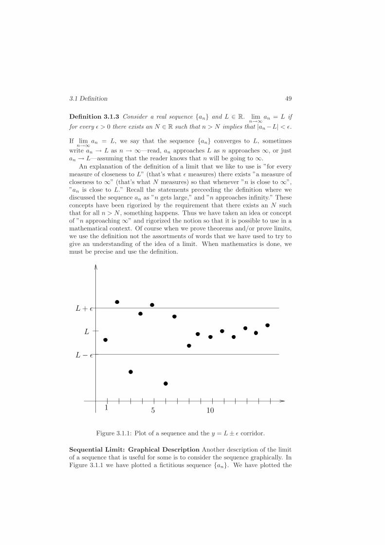
3.1 Definition 49
Definition 3.1.3 Consider a real sequence {an} and L ∈ R. limn→∞
an = L if
for every ǫ > 0 there exists an N ∈ R such that n > N implies that |an−L| < ǫ.
If limn→∞
an = L, we say that the sequence {an} converges to L, sometimes
write an → L as n → ∞—read, an approaches L as n approaches ∞, or justan → L—assuming that the reader knows that n will be going to ∞.
An explanation of the definition of a limit that we like to use is ”for everymeasure of closeness to L” (that’s what ǫ measures) there exists ”a measure ofcloseness to ∞” (that’s what N measures) so that whenever ”n is close to ∞”,”an is close to L.” Recall the statements preceeding the definition where wediscussed the sequence an as ”n gets large,” and ”n approaches infinity.” Theseconcepts have been rigorized by the requirement that there exists an N suchthat for all n > N , something happens. Thus we have taken an idea or conceptof ”n approaching ∞” and rigorized the notion so that it is possible to use in amathematical context. Of course when we prove theorems and/or prove limits,we use the definition not the assortments of words that we have used to try togive an understanding of the idea of a limit. When mathematics is done, wemust be precise and use the definition.
5
L − ǫ
L
L + ǫ
1 10
Figure 3.1.1: Plot of a sequence and the y = L± ǫ corridor.
Sequential Limit: Graphical Description Another description of the limitof a sequence that is useful for some is to consider the sequence graphically. InFigure 3.1.1 we have plotted a fictitious sequence {an}. We have plotted the

50 3. Limits of Sequences
point (0, L) and horizontal dashed lines coming out of the points (0, L± ǫ). Thecorridor within the dashed lines represents y-coordinate values that are closeto L (for a given ǫ). The definition of lim
n→∞an = L requires that for any ǫ (no
matter how large or how small you make the corridor around L—the corridorbeing small is usually the problem) there must be a value of n, call it N , so thatfrom that point on, all of the points are within the given corridor. In general,when the corridor is smaller (the ǫ is smaller), the N must get larger.
Comments: Sequential Limits (i) Given a sequence {an}, the definitiondoes not help you decide what L should be—but of course it is necessary tohave this L to apply the definition. One way to think about it is that you haveto ”guess the L” and then try to prove that the limit is L. Really we know thatwe have methods for determining L from our basic calculus course (the methodswere not rigorously proved but surely would be sufficient to guess what L shouldbe). We will repeat these results (rigorously) in later sections.
(ii) We emphasize that the value N can be any real number. By notation(an N usually represents an integer) we imply that N is an integer. It alwayscan be chosen as an integer but need not be. It is sometimes more convenient tochoose N as a particular real number rather than go through the song and dancethat it is the next largest integer greater than some particular real number–wewill make this clear later.
(iii) We want to emphasize (and we will beat this to death) that when weapply Definition 3.1.3 we will always follow two steps. Step 1: For a givenǫ define N . How we find N is immaterial–we will develop methods for findingN . Step 2: Show that the defined N works.—that n > N implies that|an − L| < ǫ. We will repeat and emphasize this procedure often.
(iv) We note that the definition of a limit can be given in terms of neigh-borhoods introduced in Section 2.2. The statements ”there exists an ǫ > 0” and”|an − L| < ǫ” (and their use) can be replaced by ”there exists a neighborhoodof L, Nǫ(L)” and ”an ∈ Nǫ(L)”. We can also define a neighborhood of infinity(even though infinity is not in R) as follows.
Definition 3.1.4 A neighborhood of infinity, ∞, is the set NR(∞) = {x ∈ R :x > R} for some R > 0. A neighborhood of minus infinity, −∞, is the setNR(−∞) = {x ∈ R : x < −R} for some R > 0.
We can then write Definition 3.1.3 as follows: limn→∞
an = L if for every neigh-
borhood of L, Nǫ(L), there exists a neighborhood of infinity, NN (∞), such thatn ∈ NN (∞) ⇒ an ∈ Nǫ(L). Other than notation there is no difference betweenthis version of the definition and the one given in Definition 3.1.3.
(v) In addition to being able to write Definition 3.1.3 in terms of neighbor-hoods we get results connecting limit points of sets and limits of sequences.
Proposition 3.1.5 Suppose {an} is a real sequence and limn→∞
an = L.
(a) Any neighborhood of L, Nr(L), contains infinitely many points of the se-quence {an}.

3.2 Applications of the Definition 51
(b) If we consider E = {a1, a2, a3, · · · } as a subset of R (instead of as a sequence)and E is an infinite set (the an’s do not all equal L from some point on), thenL is a limit point of E.
Proof: The proofs of both parts are very easy. (a) We know by Definition 3.1.3that for any neighborhood of L, Nr(L), there exists an N and all of the pointsof {an} for n > N are in that neighborhood. Note that for all we know all ofthese sequence values could be the same—say if the sequence was a constantsequence.
(b) If we consider any neighborhood of L, Nr(L), and apply the definition ofthe limit of a sequence to the sequence {an}, then the neighborhood Nr(L) willsurely contain at least one point of E. Since we have assumed that the set E isinfinite, we can find a point in Nr(L) ∩ E that is different from L.
Note that it is important for part (b) to assume that the set E is infinite.For the sequence {an} where an = 1 for n, then an → 1 but 1 is not a limitpoint of the set {a1, a2, · · · } = {1}.
When you think about the definition of the limit of a sequence—or the graphof a sequence—the above result is not surprising. The other direction—and it’snot really a converse—is a bit more of a surprise.
Proposition 3.1.6 Suppose that E ⊂ R and the point x0 is a limit point of E.Then there exists a sequence of points {xn} ⊂ E such that xn → x0.
Proof: We have essentially already proved this result. In the proof of Theorem2.3.8 we consider the sequence of neighborhoods of x0, N1/n(x0), n = 1, 2 · · ·and chose a point from each neighborhood, xn ∈ N1/n(x0). Clearly |xn − x0| <1/n for all n. Then for any ǫ > 0 we can use Corollary 1.5.5–(b) to obtainN ∈ N such that 1
N < ǫ. (Step 1: Define N .) Then for n > N we have|xn − x0| < 1
n < 1N < ǫ. (Step 2: Show that the defined N works.) Thus
limx→∞
xn = x0.
Thus we see that when E is a bigger set (has many points), if x0 is a limitpoint of E, we can always find a sequence of points of E converging to x0. Forexample if E = [0, 3/2), 3/2 is a limit point of E and xn = 3
2 + 14n → 3
2 . Also1 is a limit point of E and xn = 1 + 1
2n → 1. And 2 is a limit point of E and2 − 1
n → 2.Note that the sequence produced by the proof of Theorem 2.3.8 is such that
xn 6= x0 for any n. This is not necessary for this proof.Of course we need some experience with proving limits—finding the N and
showing that it works. We will do that in the next section.
3.2 Applications of the Definition of a Sequen-
tial Limit
In the last section we introduced the definition of a sequential limit. In thissection we will learn how to apply the definition to particular sequences. Re-

52 3. Limits of Sequences
member, we will always be following the two steps, Step 1: Define N and Step 2:Show that the N works. Let us begin with the following example. It is probablythe second easiest example possible but it is very important.
Example 3.2.1 Prove that limn→∞
1
n= 0.
Solution: We will first do this problem graphically. Generally this is not the way toprove limits—it only works for easy problems. However we want to illustrate how it workswith the picture and eventually to make a point. We note that in Figure 3.2.1 that thesequence {1/n} is plotted and the dashed lines y = 0 ± ǫ = ±ǫ are drawn. We notice thatthe sequence decreases as n gets larger (it’s easy to see that for n > m, 1/n < 1/m). After
L + ǫ
1 105L − ǫ
1
Figure 3.2.1: Plot of a sequence {1/n} and the y = L± ǫ corridor.
a while—exaggerated on this plot—the points representing the plot of the sequence enter thecorridor formed by y = ±ǫ and never leave it. The points will never leave the corridor becausethey are positive and decreasing. It is of interest to see if we can compute when the points will
cross the line y = ǫ. We set1
n= ǫ and solve for n as n = 1/ǫ. Of course ǫ would have to be
special for 1/ǫ to be an integer. However, it should be clear that if we set N = 1/ǫ (This is thedefinition of N required by Step 1: we did it graphically, but we don’t really care how we gotit.), then if n > N , we note in our plot that the plotted values of 1/n have entered into the ±ǫcorridor and because 1/n < ǫ (because n > N = 1/ǫ) and 1/n > 0, these plotted values willnever leave the ±ǫ corridor, i.e.
∣
∣
1n
∣
∣ < ǫ. (This shows that the N defined as N = 1/ǫ works:
Step 2.) Hence, we have defined an N such that if n > N = 1/ǫ, then
∣
∣
∣
∣
1
n− 0
∣
∣
∣
∣
< ǫ. Therefore
by the definition of limit, Definition 3.1.3, limn→∞
1
n= 0. Likewise, we could complete Step 2
3.2 Applications of the Definition 53
by noting if n > N = 1/ǫ, then
∣
∣
∣
∣
1
n− 0
∣
∣
∣
∣
=1
n<
1
N= ǫ. (This also shows that the N works:
Step 2.)The second way we will do this problem is the way that limit proofs are most often done.
We suppose that ǫ > 0 is given. We need N so that n > N implies that
∣
∣
∣
∣
1
n− 0
∣
∣
∣
∣
=1
n< ǫ.
This last inequality is equivalent to n > 1/ǫ. Therefore if we choose N = 1/ǫ (definition of
N : Step 1), then n > N = 1/ǫ implies that
∣
∣
∣
∣
1
n− 0
∣
∣
∣
∣
=1
n<
1
N= ǫ (Step 2: The defined N
works.). Therefore1
n→ 0 as n → ∞.
Notice that in each method, the first graphically and the second algebraically,we define N and then show that this N works—satisfies the definition of thelimit. This is always the way limit proofs are done when we are applying thedefinition of the limit. The first method illustrates that it really makes nodifference how you find N . If we can show rigorously that a particular Nworks—even if we only guessed it—we are done.
And finally, we note that the N that we found, N = 1/ǫ, depended on ǫ.This is perfectly permissable. The statement in the definition is that ”for everyǫ > 0 there exists an N .” The same N surely does not have to work for allǫ. It is logical that N would generally have to depend on ǫ (it surely is not arequirement) and with this dependence, we can still satisfy the definition. Weshould understand that generally N will depend on ǫ in a way that as ǫ getssmaller, N will get larger—as with N = 1/ǫ.
Example 3.2.2 Prove that limn→∞
[
1 − 1
n2
]
= 1.
Solution: Again, we assume that we are given ǫ > 0. We want an N such that n > N
implies
∣
∣
∣
∣
[
[1 − 1
n2
]
− 1
∣
∣
∣
∣
=
∣
∣
∣
∣
− 1
n2
∣
∣
∣
∣
=1
n2< ǫ. This last inequality is equivalent to n2 > 1/ǫ or
n >√
1/ǫ = 1/√
ǫ (because n > 0). Thus if we choose N = 1/√
ǫ (or 1/N2 = ǫ) (Define N :
Step 1) and let n > N , we have
∣
∣
∣
∣
[
[1 − 1
n2
]
− 1
∣
∣
∣
∣
=
∣
∣
∣
∣
− 1
n2
∣
∣
∣
∣
=1
n2<
1
N2= ǫ (Step 2: N works)
or limn→∞
[
1 − 1
n2
]
= 1.
You should note the proof of a limit involves the first step, where we set|an − L| < ǫ and solve this inequality of n. This shows us how we should defineN–by setting the inequality we want to be satisfied as true, we are able to seewhat we need to make it true–this is sort of a ”mathematical limits matingdance” and is not technically not a part of the proof. It is a very commonapproach to help find N . We then show that this N works. And we emphasize,after we perform the first step and define N , we always must show that Nsatisfies the definition of a limit. If you understand all of the parts of the dance,this is often easy.
Also, as a part of the analysis above we first had an inequality n2 > 1/ǫand took the square root of both sides. As a part of solving the inequality forn, we often have to perform operations on both sides of an inequality. Thequestion is why can you take the square root of both sides (or perform someother operation on both side of an inequality)? In the case of the square root,

54 3. Limits of Sequences
we proved that it was permissible in HW1.3.3–(b). To help us in general we saythat a function g defined on an interval of the real line is said to be increasingif x < y implies that g(x) < g(y). We know that g(x) =
√x is increasing–if
not because of HW1.3.3–(b), because we know what the graph of y =√x looks
like. So if x < y, then√x <
√y, i.e. you can take the square root of both
sides of an inequality. Later we had n > N = 1/√ǫ and squared both sides.
This is possible because g(x) = x2 is an increasing function also (or we can useHW1.3.3–(a)).
Example 3.2.3 Prove that limn→∞
2n + 3
5n + 7=
2
5.
Solution: Suppose that ǫ > 0 is given. We want to find an N such that n > N implies that∣
∣
∣
∣
2n + 3
5n + 7− 2
5
∣
∣
∣
∣
< ǫ, or
∣
∣
∣
∣
5(2n + 3) − 2(5n + 7)
5(5n + 7)
∣
∣
∣
∣
=
∣
∣
∣
∣
1
5(5n + 7)
∣
∣
∣
∣
=1
5
1
5n + 7< ǫ.
This inequality is the same as 5n + 7 > 1/(5ǫ) or n >1
5
(
1
5ǫ− 7
)
, i.e. we have done the
dance. Define N =1
5
( ǫ
5− 7
)
(Step 1: Define N). Then if n > N =1
5
(
1
5ǫ− 7
)
, we get
5n + 7 > 1/(5ǫ) or1
5
1
5n + 7< ǫ. Therefore n > N implies
∣
∣
∣
∣
2n + 3
5n + 7− 2
5
∣
∣
∣
∣
< ǫ (Step 2: N
works), and2n + 3
5n + 7→ 2
5as n → ∞.
Before we move on to limits that do not exist, we prove one more limit.We emphasize that we are cheating. As a part of the next example we willuse the natural logarithm, ln and the exponential, exp. We will define thesefunctions and prove properties of the ln and exp functions in Chapter 5 (or 6).We could wait for this example until then but are probably better served doingit now—there are no circular arguments involved.
Example 3.2.4 Prove that limn→∞
1
2n= 0.
Solution: We proceed as we did in the last example. We suppose that we are given ǫ > 0
and we need to find N such that n > N implies that
∣
∣
∣
∣
1
2n− 0
∣
∣
∣
∣
=1
2n< ǫ. This last inequality
is equivalent to 2n > 1/ǫ. Taking the logarithm base e of both sides gives (because ln is anincreasing function) ln 2n = n ln 2 > ln (1/ǫ) = − ln ǫ or n > − ln ǫ/ ln 2.
Thus we see that if we choose N = − ln ǫ/ ln 2 (Step 1: Define N) and consider n > N ,then we have n > N = − ln ǫ/ ln 2 or n ln 2 = ln 2n > − ln ǫ = ln (1/ǫ). Taking the exponential
of both sides, we get 2n > 1/ǫ,1
2n< ǫ or
∣
∣
∣
∣
1
2n− 0
∣
∣
∣
∣
< ǫ (N works: Step 2), and therefore1
2n
approaches 0 as n approaches ∞.
We note that we can take the ln and exp of both sides of the inequalitybecause they are both increasing functions–cheating again, but think of thegraphs of these functions and it will be clear that they are increasing.
You should also note that we have used the fact that ln 2 ≈ .69 > 0 al-lowing us to divide both sides of the inequality by ln 2 keeping the directionof the inequality the same. Also note that we write the definition of N as

3.2 Applications of the Definition 55
N = − ln ǫ/ ln 2. This is a logical way to write it because for ǫ small (less than1 but positive), ln ǫ < 0. But do note that nothing we have done is illegal if ǫ isnot small, say ǫ ≥ 1. The definition must be satisfied for all ǫ > 0.
Sequences that don’t converge It should not surprise you that there aresequences that do not have limits. Here we want to discuss how lim
n→∞an does
not exist for some sequences and what we have to do to prove that a limit doesnot exist. If you think about it, you should realize that it might be difficult toshow that the limit does not exist. You have to show that it is impossible tosatisfy the definition no matter what real L you choose, i.e. we have to showthat for any L ∈ R there exists an ǫ for which no N can be found (no N suchthat n > N implies that |an − L| < ǫ). There are generally two ways thatthe limit does not exist. We have put the requirement in Definition 3.1.3 thatL ∈ R and we know that ±∞ 6∈ R. Therefore, the sequences that want toapproach ∞ (or −∞) such as the sequence given in Section 3.1,
{
n2 + 1}∞n=0
,will not satisfy Definition 3.1.3. (We will give a definition later for what wemean when the limit is infinite.) The other case where the limit does not existsis when it oscillates back and forth between two distinct numbers–or close totwo distinct numbers, or three. The literature seems to be confusing on howthey refer to the two situations of non-convergence. At the moment we will saythat if a sequence does not satisfy Definition 3.1.3 for any L ∈ R, the sequencedoes not converge (that’s the only convergence definition we have at this time).Some of the literature will refer to non-convergence as divergence. We will savedivergence for limits of ±∞ which we will introduce when we introduce infinitelimits (but at this time do not exist). Consider the following example.
Example 3.2.5 Prove that limn→∞
n2 + 1 does not exist.
Solution: This is really a fairly easy case. Let L be any element of R and choose ǫ = 1. Notethat from what we said above, if no N can be found for this situation (any L ∈ R and one ǫ),then the limit will not exist. If we were to be able to satisfy the definition, we must satisfy thefollowing inequality,
∣
∣n2 + 1 − L∣
∣ < 1. This inequality is the same as L− 1 < n2 + 1 < L + 1.Hopefully, it is clear that it is the right inequality that will not be satisfied for large n—youshould notice that for some value of n, n2 + 1 will get larger than L + 1 and stay larger forall of the rest of the n’s. Rewrite the right inequality as n2 < L or n <
√L (allowable since
n > 0).
By Corollary 1.5.5–(a) we know that for√
L ∈ R, there exists n0 ∈ N such that n0 >√
L.Of course, if this inequality is satisfied for some particular n0 ∈ N, it will also be satisfied forall n ≥ n0. Since it is impossible to find an N such that n > N implies n <
√L (because for
all n ≥ n0, n >√
L), it is impossible to find an N such that n > N implies∣
∣n2 + 1 − L∣
∣ < 1
for any L ∈ R. Since Definition 3.1.1 cannot be satisfied for any L ∈ R, limn→∞
n2 + 1 does not
exist.
Note that when we wrote√
L, we were assuming that L ≥ 0. If someone is silly enoughto guess that the limit might be L where L < 0, it is easy to see that n2 +1 6< L+1 (the rightside of the original inequality) for all n ∈ N, n ≥ 1. Therefore the limit can’t be negative.
The above example is a reasonably easy sequence to consider—however, allmore complicated sequences that approach ∞ (or −∞) are handled in the sameway with more difficult algebra.
56 3. Limits of Sequences
We next consider an example that is a classic case of nonexistence. All otherexamples of nonexistence where the sequence oscillates between one or moredifferent values can be done in a similar fashion.
Example 3.2.6 Prove that limn→∞
(−1)n does not exist.
Solution: As in the last example we must show that for any L ∈ R, there is an ǫ > 0 forwhich no N exists (no N such that n > N implies that |an − L| < ǫ). For whatever ever realnumber L we think that might be the limiting value, we must satisfy |(−1)n − L| < ǫ or
L − ǫ < (−1)n < L + ǫ. (3.2.1)
And if the sequence is to have a limit, we must find an N so that the last inequality is satisfiedfor all n > N .
If you were trying to guess the limit and were naive enough to think that the limit wouldexist, you might guess that the limit is 1 or you might guess that it is −1. After all, these arethe values that are assumed often in this sequence.
If we choose L = 1 (as our first guess) and set ǫ = 1, then we would have to satisfy theinequality (3.2.1), 1 − 1 = 0 < (−1)n < 1 + 1 = 2. It should be clear that this inequalitycannot be satisfied for any odd values of n when (−1)n = −1. Therefore it is impossible tofind an N so that n > N implies 0 < (−1)n < 2.
Likewise if we were to choose L = −1 and ǫ = 1, the inequality −2 < (−1)n < 0 wouldnot be satisfied for even values of n so no appropriate N can be defined. Therefore lim
n→∞(−1)n
does not equal 1 or −1.Finally, consider some L such that L 6= 1 and L 6= −1. Choose ǫ = min{|L − 1|/2, |L −
(−1)|/2} (where by min{|L − 1|/2, |L − (−1)|/2} we mean the minimum of the two values).You might want to draw a picture describing this choice. It should be clear that this ǫ hasbeen chosen so that |(−1)n − L| is never less than ǫ for any n—when n is even |(−1)n −L| =
|1 − L| >|1 − L|
2≥ ǫ and when n is odd |(−1)n − 1| = | − 1 − L| >
|1 + L|2
≥ ǫ. Therefore
limn→∞
(−1)n does not equal L (where L is anything but 1 or −1).
Therefore, since Definition 3.1.3 cannot be satisfied with any L ∈ R, limn→∞
(−1)n does not
exist.
We should note that both of these cases of nonexistence of limits can be illus-trated graphically—you should be very careful before you claim that the picturegives you a proof. You will be asked to graphically illustrate the nonexistence ofseveral limits of sequences in HW3.2.2. In Figure 3.2.2 we draw a picture muchlike we did in Figure 3.1.1—choose some L and ǫ, plot the point (0, L) and drawthe lines y = L± ǫ. To illustrate the non-existence in Example 3.2.5 we choosean arbitrary L and let ǫ = 1. We then plot some sequence values an = n2 + 1.We note that sooner or later the sequence points go outside of the y = L ± ǫcorridor (actually above the corridor) and stay out of there forever—we did notget to plot many points in Figure 3.2.2 because n2+1 grows large quickly. Sincethe sequence clearly leaves the L ± ǫ-corridor and never comes back, the limitis surely not equal to L.
To illustrate the non-existence in Example 3.2.6 we would draw two plotssimilar to that in Figure 3.1.1. For the first plot, Figure 3.2.3, we would chooseL = 1 and ǫ = 1/2, and note that every other point of the sequence ((−1)n forn odd) would be outside of the y = 1 ± 1/2 corridor–forever. We could drawa similar plot for L = −1—and make a similar argument. In Figure 3.2.4 wedraw a plot for an arbitrary L not equal to 1 or −1 and choose ǫ to be smaller

3.2 Applications of the Definition 57
L
1 105
L + ǫ
L − ǫ
Figure 3.2.2: Plot of a sequence {n2 + 1} and the y = L± 1 corridor.
5
1 10
-1
L+1/2
L-1/2-
1
Figure 3.2.3: Plot of a sequence {(−1)n} and the y = 1 ± 1/2 corridor.

58 3. Limits of Sequences
5 101
−1
L + ǫ
L − ǫL
1
Figure 3.2.4: Plot of a sequence {(−1)n} and the y = L ± ǫ corridor whereǫ < min{|L− 1|, |L− (−1)|}.
than the distances from L to 1 or −1. We note that the sequence values wouldnever be in the y = L± ǫ-corridor.
As stated earlier be very careful about claiming that the above argumentsare proofs. They can be made to be a part of a proof if done carefully and ifthey include some of the arguments are reasons given in Examples 3.2.5 and3.2.6. The pictures alone are at best ”bad proofs.”
We see from the work in this section that it is not trivial to apply thedefinition of the limit of a sequence. You might wonder if it’s because wehave the wrong definition. So that we have the definition here for comparisonpurposes, we recall that lim
n→∞an = L
if for every ǫ > 0 there exists N such that n > N implies |an − L| < ǫ.
One might ask if it is necessary to apply the definition so that it works for everyǫ > 0. We might try the following candidate for the definition.
F1: if for some ǫ > 0 there exists N such that n > N implies |an − L| < ǫ.
If this were the definition, life would be much easier. Consider an =1
nand
choose ǫ = 0.1. If we choose N = 13, then n > N = 13 implies that∣
∣
∣
∣
1
n− 0
∣
∣
∣
∣
=1
n<
1
N=
1
13< 0.1.
If F1 were the definition, the above computation would imply that limn→∞
1
n= 0.
This is the same result that we got in Example 3.2.1 (which we hope our intuition

3.2 Applications of the Definition 59
tells us is the correct limit). We see that F1 is easy to apply. However, usingthe same ǫ = 0.1 we see that if we choose N = 100, then n > N = 100 impliesthat
∣
∣
∣
∣
1
n− 0.001
∣
∣
∣
∣
≤ 1
n+ 0.001 < 0.01 + 0.001 < 0.1.
So the same ǫ would imply that limn→∞
1
n= 0.001. Further calculations using
F1 would give as a large assortment of answers for limn→∞
1
n(this makes it very
difficult to grade homework). And different choices of ǫ would give us morevalues of the limit. Clearly F1 is a bad choice—it is not a strong enough criterionto serve as our definition.
If we instead tried
F2: if for every ǫ > 0 and all N ∈ N, n > N implies |an − L| < ǫ.
This proposal is in big trouble. Here we are claiming that for any ǫ > 0, theimplication in the definition must be true for all N . That is just too strong of arequirement. If we return to an = 1/n and choose a small ǫ, say ǫ = .1, there is
not way that n > N = 1 will imply that
∣
∣
∣
∣
1
n− 0
∣
∣
∣
∣
< 0.1, i.e. for n = 2 > N = 1,∣
∣
∣
∣
1
n− 0
∣
∣
∣
∣
=1
2> 0.1. So either lim
n→∞1
n6= 0 or F2 will not make it as a definition
replacement.
There are a few other candidates—bad candidates—that we could discussbut by now you surely get the point, we had better live with Definition 3.1.3.You will see in the next section that using Definition 3.1.3 we will always get aunique result—not like F1. We have seen that it is possible to apply Definition3.1.3 to prove limits that are intuitively correct—not like F2. So make sure thatyou now forget F1 and F2: the F stood for ”false”.
And finally, we want to emphasize that it is the tail end of the sequencethat determines whether or not the sequence converges—and since n → ∞, nomatter at which number you start the tail, it will be a very long tail. In the firstexample of this section we showed that 1/n → 0 as n → ∞. That makes thesequence {1/n} a nice sequence. In the last example of this section we showedthat lim
n→∞(−1)n does not exist, i.e. the sequence {(−1)n} is not a nice sequence.
Now let us construct a rather strange sequence by defining an = (−1)n forn = 1, · · · , 100, 000 and an = 1/n for n > 100, 000. The tail end of the sequencewill be nice so that the sequence will converge—again to 0. Specifically we sawin Example 3.2.1 that as a part of the proof of the convergence of {1/n} to0, we defined N = 1/ǫ. To prove that the sequence {an} converges to 0, wedefine N = max{1/ǫ, 100, 000}. This way the proof never knows that we wereworking with a strange sequence. If we define a sequence {bn} by bn = 1/nfor n = 1, · · · , 100, 000, 000 and bn = (−1)n for n > 100, 000, 000, then lim
n→∞bn
does not exist (after a long time the sequence values will start bouncing back

60 3. Limits of Sequences
and forth between 1 and −1 and do that for ever. If the tail end of a sequenceis bad, the sequence will be bad.
HW 3.2.1 (True or false and why.)
(a) Suppose that the sequence {an} is such that |an − 7| < 1
nfor all n ∈ N.
Then limn→∞ an = 7.(b) Consider the sequence {an}, n = 1, 2, · · · where an = c ∈ R for all n (i.e.the sequence c, c, c, · · · ). Then lim an = c.
HW 3.2.2 (a) Consider the sequence
{
2n2 + 4
n+ 3
}∞
n=1
. Illustrate graphically
that limn→∞
2n2 + 4
n+ 3does not exist.
(b) Consider the sequence
{
(−1)n +1
n
}∞
n=1
. Illustrate graphically that limn→∞
[
(−1)n +1
n
]
does not exist.
(c) Prove that limn→∞
[
(−1)n +1
n
]
does not exist, i.e. use the definition).
HW 3.2.3 (a) Prove that the limit limn→∞
2n2 + 4
3n2 + 1=
2
3(use the definition).
(b) Prove that the limit limn→∞
2n2 + 4
3n2 + n+ 1=
2
3(use the definition).
HW 3.2.4 Suppose that {an} and {bn} are sequence such that limn→∞
an =
limn→∞
bn = 0. Prove that limn→∞
anbn = 0.
3.3 Some Sequential Limit Theorems
We want to be able to compute limits and know what we have computed is thecorrect result but we do not want to have to apply the definition every time.Hence we now want to move on to the propositions, theorems and corollaries(all referred to collectively as theorems) concerning limits of sequences. Youprobably already know most of these theorems from your basic calculus course.Most of these theorems are the building blocks that allow you to compute thelimit of a sequence without using the definition—but as you will see, the defini-tion of a limit is the core of the proof of all of these theorems. The limits thatwe compute using the limit theorems will be as rigorous as the limits that wehave proved using the definition because all of the results that we use will havebeen rigorously proved.
We begin with a discussion of one of the common hypotheses of the theorems.We note in Proposition 3.3.1 we assume that lim
n→∞an exists. This is a common
assumption for most of the propositions in this section and the next section.What does this mean? Moreso, what do we get to use from this assumption?This is very easy—and very, very important—if we return to Defintion 3.1.3.

3.3 Some Limit Theorems 61
In the first place the hypothesis ensures us that there is some L such thatlimn→∞
an = L. For the sequence {an} and this L, the hypothesis ensures us that
for any ǫ > 0 we can find an N such that n > N implies that |an − L| < ǫ.The hypothesis doesn’t tell us what N and L are or how to find them. It justguarantees that there are such an Nand L—and that’s all we need. As we saidabove, just about every proposition in this section and the next will have thistype of hypothesis. Think clearly each time just how it’s being used.
We begin with a result that is probably unlike results you have seen beforebut is basic. From our basic calculus class we know how to compute some limits.From the last section, for a given sequence {an} and L we know how to applythe definition of a sequential limit to show that the the sequence {an} and Lsatisfy the definition. But what if after you read Example 3.2.3 and gain an
understanding how Definition 3.1.3 was used to show that limn→∞
2n+ 3
5n+ 7=
2
5,
one of your classmates says that the limit is really 5/2 and claims that she canapply Definition 3.1.3 to prove it. Could the text (and your reading of the text)and your classmate both be right? Has it been made clear that a sequence can’thave two distinct limits that satisfy the definition? We answer these questionswith the following proposition.
Proposition 3.3.1 Suppose {an} is a real sequence and limn→∞
an exists. The
limit is unique.
Proof: A common way to prove uniqueness is to use contradiction. Thuswe assume that the above statement is false, i.e. we assume that there existsL1, L2 ∈ R such that L1 6= L2, lim
n→∞an = L1 and lim
n→∞an = L2. By these
assumptions we know that for any ǫ1 > 0 there exists an N1 such that n > N1
implies |an − L1| < ǫ1, and for any ǫ2 > 0 there exists an N2 such that n > N2
implies |an − L2| < ǫ2. Another way to write this is for n > N1, L1− ǫ1 < an <L1 + ǫ1, and for n > N2, L2 − ǫ2 < an < L2 + ǫ2.
To help see why this assumption is clearly false, we have included the plotin Figure 3.3.1. Since L1 6= L2, we have choosen ǫ1 and ǫ2 sufficiently small sothat the L1 ± ǫ1 and L2 ± ǫ2-corridors do not intersect. Yet for all n > N1 all ofthe values an must be in the L1± ǫ1-corridor and for n > N2 all of the values anmust be in the L2 ± ǫ2-corridor—we try to illustrate this in the plot but it isn’tgoing to happen—the question marks signify the fact that we can’t put them inboth places.
For the proof we set ǫ1 = ǫ2 = |L1 − L2| /2. For convenience and withoutloss of generality, we assume that L1 > L2 so ǫ1 = ǫ2 = (L1 − L2) /2—one ofthe two values must be larger than the other. Define N = max{N1, N2}. Thenfor all n > N (so that n > N1 and n > N2) we will have
L1 − ǫ1 = (L1 + L2)/2 < an < L1 + ǫ1 = (3L1 − L2)/2 (3.3.1)
and
L2 − ǫ2 = (3L2 − L1)/2 < an < L2 + ǫ2 = (L1 + L2)/2. (3.3.2)

62 3. Limits of Sequences
?
?
? ?
? ?L1 − ǫ
L1
L1 + ǫ
L2 − ǫL2
L2 + ǫ
Figure 3.3.1: Plot of the y = L1 ± ǫ and L2 ± ǫ corridors, and some sequencepoints—trying to be in both corridors.
The left most inequality in statement (3.3.1 and the right most inequality instatement (3.3.2 gives us for all n > N = max{N1, N2}
(L1 + L2)/2 < an < (L1 + L2)/2. (3.3.3)
This is surely a contradicition. Therefore no such L1 and L2 exists, and thelimit is unique.
Hence we see that if such a claim about the results of Example 3.2.3 ismade, either the text or your classmate must be wrong (and we’re betting onthe classmate).
We next state and prove a proposition that includes several of our basicsequential limit theorems.
Proposition 3.3.2 Suppose that {an} and {bn} are real sequences, limn→∞
an =
L1, limn→∞
bn = L2 and c ∈ R. We then have the following results.
(a) limn→∞
(an + bn) = L1 + L2.
(b) limn→∞
can = c limn→∞
an = cL1.
(c) There exists an K ∈ R such that |an| ≤ K for all n.(d) lim
n→∞(anbn) = L1L2.
Proof: (a) Suppose ǫ > 0 is given. The first two hypotheses gives us that
for any ǫ1 > 0 there exists an N1 such that n > N1 implies that |an − L1| < ǫ1,(3.3.4)
and
for any ǫ2 > 0 there exists an N2 such that n > N2 implies that |bn − L2| < ǫ2.(3.3.5)

3.3 Some Limit Theorems 63
We note that
|(an + bn) − (L1 + L2)| = |(an − L1) + (bn − L2)| ≤ |(an − L1)| + |(bn − L2)| ,(3.3.6)
where the last inequality follows from the triangular inequality, Proposition1.5.8–(v). Define ǫ1 = ǫ2 = ǫ/2 (the hypotheses presented in (3.3.4) and (3.3.5)allow for any ǫ1 and ǫ2), N = max{N1, N2} (Step 1: Define N) and let n > N(so that the last inequalities in both (3.3.4) and (3.3.5) will hold true). Thenfrom inequality (3.3.6) we get
|(an + bn) − (L1 + L2)| ≤ |(an − L1)| + |(bn − L2)| <ǫ
2+ǫ
2= ǫ
(Step 2: Show that the defined N works). Then by Definition 3.1.3 an + bn →L1 + L2 as n→ ∞.
(b) We begin by noting that if c = 0 the result is very easy because the sequence{can} will be the zero sequence and c lim
n→∞an will be zero—the result then
follows from HW3.2.1-(b).Hence, we assume that c 6= 0. We suppose that we are given an ǫ > 0. The
hypothesis that limn→∞
an = L1 gives us that for any ǫ1 > 0 there exists anN1 ∈ R
such that n > N1 implies |an − L1| < ǫ1. We need anN such that n > N impliesthat |can − cL1| < ǫ. By Proposition 1.5.8–(ii) this last inequality is the same as|c| |an − L1| < ǫ. Thus we see that if we apply our hypothesis with ǫ1 = ǫ/|c| andN = N1, for n > N we have |can − cL1| = |c| |an − L1| < |c|ǫ1 = |c|(ǫ/|c|) = ǫ.Therefore by Definition 3.1.3 lim
n→∞can = cL1.
(c) This statement is clearly different from parts (a), (b), and (d). As we shallsee, this result is both a very important tool and generally a very importantproperty of convergent sequences. We begin by choosing ǫ1 = 1 and apply thehypothesis that lim
n→∞an = L1 to get an N1 ∈ R such that n > N1 implies that
|an − L1| < ǫ1 = 1. Then by this last inequality and the backwards triangularinequality, Proposition 1.5.8–(vi), we have for n > N1
|an| − |L1| ≤ |an − L1| < ǫ1 = 1,
or |an| < |L1| + 1. This inequality bounds most of the sequence {an}. If we letN0 = [N1] where the bracket function is defined by [x] is the largest integer lessthan or equal to x, then inequality |an| < |L1| + 1 for n > N1 bounds |an| forn = N0 + 1, N0 + 2, · · · . Thus we set K = max{|a1|, |a2|, · · · , |aN0
|, |L1| + 1}and we have our desired result.
We note that in the above proof it would have been convenient if we hadalways defined N to be a natural number (so that we didn’t have to use the[N ]). However, we have had many instances when it has been convenient forus to only require that N ∈ R. We should also note that it is the completenessaxiom that assures us that such an integers N0 exists. We are defining [N ] to bethe least upper bound of the set {n ∈ N : n ≤ N}—which surely exists becausethe set is bounded above by N .
64 3. Limits of Sequences
(d) Suppose ǫ > 0 is given. The first two hypotheses give us that
for any ǫ1 > 0 there exists an N1 such that n > N1 implies that |an − L1| < ǫ1,(3.3.7)
and
for any ǫ2 > 0 there exists an N2 such that n > N2 implies that |bn − L2| < ǫ2.(3.3.8)
We must find an N such that n > N implies that |anbn − L1L2| < ǫ. It shouldnot surprise you that the proof will be similar to that given in part (a)—with adifferent dance. We note that
|anbn − L1L2| = |(an(bn − L2) + L2(an − L1)| ≤ |an(bn − L2)| + |L2(an − L1)|= |an| |(bn − L2)| + |L2| |(an − L1)| . (3.3.9)
(To verify the first step just multiply out the second expression. The firstinequality is due to the triangular inequality, Proposition 1.5.8–(v)—we will usethis often. The last step just uses |xy| = |x||y|, Proposition 1.5.8–(ii).) Thenstarting with expression (3.3.9) and using (3.3.7), n > N1, (3.3.8), n > N2 andpart (c) of this proposition, we get
|anbn − L1L2| ≤ |an| |(bn − L2)| + |L2| |(an − L1)| < Kǫ2 + |L2| ǫ1. (3.3.10)
Thus we see that if we choose ǫ2 = ǫ/2K, ǫ1 = ǫ/2|L2| and N = max{N1, N2}(so that both of the inequalities in (3.3.7) and (3.3.8) are satified), we have|anbn − L1L2| < ǫ whenever n > N . Therefore lim
n→∞anbn = L1L2.
We should note that when many mathematicians are doing proofs such asthis one, they will often let ǫ1 = ǫ2 = ǫ, obtain expression (3.3.10) (with ǫreplacing ǫ1 and ǫ2) and claim that they are done. And they are. The last termof expression (3.3.9) would be (K+ |L2|)ǫ. Because of the ǫ we are able to make|anbn − L1L2| arbitrarily small—which is really our goal. However, we don’ttechnically satisfy Definition 3.1.3. But it should also be clear at this time thatthe (K + |L2|)ǫ term can be fixed up so as to give the desired result. Textbookswill generally fix it up so that they always end with just an ǫ at the end ofthe inequality—it’s just a bit cleaner. But don’t be surprised if you see this”sloppier” (but correct) approach in classes and talks.
We now have some of the basic results that let us compute easy limits. Weknow from Example 3.2.1 that lim
n→∞1/n = 0. It should be easy to see that
we can use part (d) of the above theorem to get limn→∞
1/n2 = 0 and another
application of part (d) will give limn→∞
1/n3 = 0. We are able to obtain the
following more general result.
Example 3.3.1 Prove that limn→∞
1
nk= 0 for any k ∈ N.
Solution: We hope that you realize that this result is a natural for mathematical induction.Step 1: Prove true for k = 1. Example 3.2.1 shows that it is true for k = 1.
3.3 Some Limit Theorems 65
Step 2: Assume true for k = j, i.e. limn→∞
1
nj= 0.
Step 3: Prove true for k = j + 1, i.e. prove that limn→∞
1
nj+1= 0. This proof is an easy
application of part (d) of Proposition 3.3.2. We write1
nj+1as
1
nj
1
n. We know from Example
3.2.1 that limn→∞
1/n = 0. We know from the inductive assumption, Step 2, that limn→∞
1
nj= 0.
Then by part (d) of Proposition 3.3.2 we have
limn→∞
1
nj+1= lim
n→∞
1
njlim
n→∞
1
n= 0.
Therefore the proposition is true for k = j + 1.By the principle of mathematical induction the proposition is true for all k ∈ N.
Note that you must be careful to not mix up the fact that usually ourstatements to be proved by math induction were given in terms of n and weused k as our dummy index. In this case, since n was already in use, ourstatement is given in terms of k and we used j as our dummy index. It can beconfusing but is only a matter of notation.
Also, we might be inclined to want to prove the above result using part (d)of Proposition 3.3.2) (k − 1 times) and Example 3.2.1 to show that
limn→∞
1
nk= lim
n→∞1
n· · · lim
n→∞1
nrepeated k times
= 0.
This is a perfectly good approach. Hopefully you realize when you include the”three dots” you are including a math induction proof in disguise—and hope-fully an easy one. The result needed here is the extension of part (d) of Propo-sition 3.3.2 that can be stated as follows. Let {ajn}∞n=1, j = 1, · · · , k denote kreal sequences such that lim
n→∞ajn = Lj for j = 1, · · · , k. Then lim
n→∞a1n · · · akn =
L1 · · ·Lk. It is hoped that you realize that this statement can be proved rea-sonably easily by mathematical induction—like the proof given above.
We next note that we can use parts (a) and (b) of Proposition 3.3.2, andExample 3.3.1 to show that
limn→∞
[
1 − 1
n2
]
= limn→∞
1+ limn→∞
(−1)1
n2= 1+ lim
n→∞(−1) lim
n→1
n2= 1+(−1)0 = 1,
which is the same result we got in Example 3.2.2. We note that once we haveproved Proposition 3.3.2, HW3.2.1-(b) and Example 3.3.1, the proof of thelimit given here is every bit as rigorous as the proof given in Example 3.2.2.In the next example we prove a more general result that can be useful. Let pdenote a k-th degree polynomial p(x) = a0x
k +a1xk−1 + · · ·+ak−1x+ak where
a0, a1, · · · , ak are real.
Example 3.3.2 Prove that
limn→∞
p(1/n) = limn→∞
[
a01
nk+ a1
1
nk−1+ · · · + ak−1
1
n+ ak
]
= ak .
66 3. Limits of Sequences
Solution: Again it should be clear that this proof could be done by induction. Instead, wewill prove this result using the extension of part (a) of Proposition 3.3.2 along with parts (b)and Example 3.2.1 to see that
limn→∞
p(1/n) = limn→∞
[
a01
nk+ a1
1
nk−1+ · · · + ak−1
1
n+ ak
]
= limn→∞
[
a01
nk
]
+ limn→∞
[
a11
nk−1
]
+ · · · + limn→∞
[
ak−11
n
]
+ limn→∞
[ak ]
= limn→∞
a0 limn→∞
1
nk+ lim
n→∞a1 lim
n→∞
1
nk−1+ · · · + lim
n→∞ak−1 lim
n→∞
1
n+ lim
n→∞ak
= ak .
This is a nice straightforward proof of the desired result but it does depend strongly onthe use of the extension of part (a) Proposition 3.3.2—which you should be confident followseasily from part (a) or you should prove it.
HW 3.3.1 (True or False and why) (a) If limn→∞
|an| exists, then limn→∞
an exists.
(b) If limn→∞
anbn
and limn→∞
bn exists, then limn→∞
an exists.
(c) If limn→∞
an exists, then limn→∞
a3n exists.
(d) If limn→∞
a3n exists, then lim
n→∞an exists.
(e) If limn→∞
anbn exist, then limn→∞
an and limn→∞
bn exist.
HW 3.3.2 Prove that if limn→∞
an = 0, then limn→∞
|an| = 0.
HW 3.3.3 Prove that if limn→∞
an = L, then limn→∞
|an| = |L|.
HW 3.3.4 Consider the sequence {an}.(a) Prove that lim
n→∞an = L if and only if lim
n→∞[an − L] = 0.
Prove that limn→∞
an = L implies that limn→∞
|an − L| = 0.
Show that limn→∞
|an − L| = 0 does not imply that limn→∞
an = L.
3.4 More Sequential Limit Theorems
As the section title indicates there are more results that we need concerningsequential limits. The first result is a very basic result that you probably alreadyknow. Hopefully sometime during your elementary calculus class you found
limits such as limn→∞
2n2 + n− 3
3n2 + 3n+ 3. You wrote
limn→∞
2n2 + n− 3
3n2 + 3n+ 3= lim
n→∞
2 + 1n − 3 1
n2
3 + 3 1n + 3 1
n2
=limn→∞
[
2 + 1n − 3 1
n2
]
limn→∞[
3 + 3 1n + 3 1
n2
] =2
3.
The first step above follows from the fact that the expressions inside of thelimit is exactly the same for the first two terms—the second term is found by
multiplying the first by1/n2
1/n2. In the second step of the calculation we would be

3.4 More Limit Theorems 67
using part (b) of Proposition 3.4.1 given below and two applications of Example3.3.2 (or in place of Example 3.3.2 you can use parts (a), (b) of Proposition3.3.2 and Example 3.3.1). Thus we next include the quotient rule for sequentiallimits.
Proposition 3.4.1 Suppose that {an} and {bn} are real sequences, limn→∞
an =
L1 and limn→∞
bn = L2. Then we have the following results.
(a) If L2 6= 0 then there exists an M ∈ R and an N3 ∈ R such that |bn| ≥ Mfor all n > N3.
(b) If L2 6= 0, then limn→∞
anbn
=L1
L2.
Proof: (a) As in the other proofs, the hypotheses for this result implies thatfor every ǫ2 > 0 there exists an N2 ∈ R so that for n > N2, |bn − L2| < ǫ2.We are also given the fact that L2 6= 0. This is another result for which it isconvenient to draw a picture. In Figure 3.4.1 we have used the fact that L2 6= 0to choose an ǫ2 so that the L2 ± ǫ2-corridor forces the sequence values to beaway from zero for all n greater than some N3, i.e. we have choosen an ǫ2 sothat y = 0 is not in the L2 ± ǫ2-corridor.
The easiest way to accomplish this is to choose ǫ2 = |L2| /2. Then thehypothesis implies that there exists an N2 ∈ R such that n > N2 implies that|bn − L2| < |L2| /2 or |L2 − bn| = |bn − L2| < |L2| /2. Then by the backwardstriangular inequality, Proposition 1.5.8–(vi), for n > N3 = N2 we get
|L2| − |bn| ≤ |L2 − bn| < |L2| /2
or |bn| > |L2| /2.
L2 + ǫ2
L2 − ǫ2
L2
Figure 3.4.1: Plot of a sequence and the y = L2 ± ǫ corridor.

68 3. Limits of Sequences
(b) Before we proceed we note that
anbn
− L1
L2=L2an − L1bn
L2bn=L2(an − L1) − L1(bn − L2)
L2bn. (3.4.1)
We note that we like the an−L1 and bn−L2 terms in the numerator because wecan make them small. The L2 and L1 are also good in the numerator becausethey’re constants. The minus sign between the two terms does not cause ustrouble because when we use the triangular inequality separate the two terms,we can use the fact that the triangular inequality will give us |x−y| = |x+(−y| ≤|x|+ |−y| = |x|+ |y|—so it’s as if the minus sign isn’t really there. The bn termin the denominator is the term that might cause us most problems but we havepart (a) of this proposition. So let’s begin.
Suppose ǫ > 0 is given. The first two hypotheses give us that
for any ǫ1 > 0 there exists an N1 such that n > N1 implies that |an − L1| < ǫ1,(3.4.2)
and
for any ǫ2 > 0 there exists an N2 such that n > N2 implies that |bn − L2| < ǫ2.(3.4.3)
Since L2 6= 0, we can apply part (a) of this proposition to get an M and N3
such that n > N3 implies |bn| ≥M . If we choose n so that n > N1, n > N2 andn > N3, i.e. choose n > N = max{N1, N2, N3}, we can return to inequality(3.4.1) to see that
∣
∣
∣
∣
anbn
− L1
L2
∣
∣
∣
∣
=∣
∣
∣
L2(an−L1)−L1(bn−L2)L2bn
∣
∣
∣≤ |L2(an−L1)|+|L1(bn−L2)|
|L2bn| (3.4.4)
= |L2||(an−L1)|+|L1||(bn−L2)||L2||bn| < |L2|ǫ1+|L1|ǫ2
|L2|M . (3.4.5)
Thus if we choose ǫ1 = Mǫ/2 and ǫ2 = M |L2| ǫ/ (2 |L1|), we can apply inequal-ities (3.4.4)–(3.4.5) to get
∣
∣
∣
∣
anbn
− L1
L2
∣
∣
∣
∣
<|L2( |Mǫ/2) + |L1| [M |L2| ǫ/ (2 |L1|)]
|L2|M= ǫ.
Therefore an/bn → L1/L2 as n→ ∞.We note that the above argument only applies if L1 6= 0 also. If L1 = 0, we
can consider inequality (3.4.4) and note that it will have only one term in thenumerator. The proof then follows as above with the same definition of ǫ1—ǫ2is not necessary in this case.
In the introduction to Proposition 3.4.1 we included a calculation using thequotient rule. To obtain a more general result we let p and q denote k-thand m-th degree polynomials p(x) = a0x
k + a1xk−1 + · · · + ak−1x + ak and
q(x) = b0xm + b1x
m−1 + · · · + bm−1x + bm, respectively, where a0, a1, · · · , akand b0, b1, · · · , bm are real. We obtain the following result.

3.4 More Limit Theorems 69
Example 3.4.1 (a) If k = m and b0 6= 0, then
limn→∞
p(n)
q(n)=
a0
b0. (3.4.6)
(b) If k < m and b0 6= 0, then
limn→∞
p(n)
q(n)= 0. (3.4.7)
(c) If k > m and bj 6= 0 for some j = 1, · · · , m, then limn→∞
p(n)
q(n)does not exist.
Solution: We want to make you very aware that in the last example we used the polynomialp and calculated a limit of p(1/n). In this example we have p(n) and q(n) in our limitstatements. As you will see we will juggle things so that we can still use the results of the lastexample—but that’s why we are getting a0 and b0 in our answer and not ak and bm.(a) (k = m)Part (a) of this result is quite easy—it can be proved precisely the way youcomputed these limits in your first calculus classes (except this time we will be using a quotientresult that we have proved). We note that
limn→∞
p(n)
q(n)= lim
n→∞
a0nk + a1nk−1 + · · · + ak−1n + ak
b0nm + b1nm−1 + · · · + bm−1n + bk
= limn→∞
a0 + a11n
+ · · · + ak−11
nk−1 + ak1
nk
b0 + b11n
+ · · · + bk−11
nk−1 + bk1
nk
multiply top and bottom by 1/nk
=limn→∞
[
a0 + a11n
+ · · · + ak−11
nk−1 + ak1
nk
]
limn→∞
[
b0 + b11n
+ · · · + bk−11
nk−1 + bk1
nk
] part (b), Proposition 3.4.1
=a0
b0by applying Example 3.3.2 twice
(b) (k < m) For this case we proceed similar to the way that we proceeded in part (a)—wewill multiply the top and bottom by 1/nm. We get
limn→∞
p(n)
q(n)= lim
n→∞
a0nk + a1nk−1 + · · · + ak−1n + ak
b0nm + b1nm−1 + · · · + bm−1n + bk
= limn→∞
a01
nm−k + a11
nm−k+1 + · · · + ak−11
nm−1 + ak1
nm
b0 + b11n
+ · · · + bk−11
nk−1 + bk1
nk
multiply by 1/nm
1/nm
=limn→∞
[
a01
nm−k + a11
nm−k+1 + · · · + ak−11
nm−1 + ak1
nm
]
limn→∞
[
b0 + b11n
+ · · · + bk−11
nk−1 + bk1
nk
]
=0
b0= 0 (by applying Example 3.3.2) twice.
(c) (k > m) This statement is true but the proof is too ugly to include here.
There are other results that we need or would like concerning limits of se-quences. We can use the definition to prove that lim
n→∞(−1)n/n converges to zero.
However a tool that can be used to prove the convergence of this limit and manyothers is the following proposition referred to as the Sandwich Theorem.
Proposition 3.4.2 Suppose that {an}, {bn} and {cn} are real sequence forwhich lim
n→∞an = lim
n→∞cn = L and an ≤ bn ≤ cn for all n greater than some N1.
Then limn→∞
bn = L.

70 3. Limits of Sequences
Proof: We suppose that we are given an ǫ > 0. The two limit hypotheses giveus that there exists an N2 such that n > N2 implies that |an − L| < ǫ, or
L− ǫ < an < L+ ǫ, (3.4.8)
and there exists an N3 such that n > N3 implies that |cn − L| < ǫ, or
L− ǫ < cn < L+ ǫ. (3.4.9)
Then if we use the left inequality of (3.4.8), the right inequality of (3.4.9) andthe hypothesis that an ≤ bn ≤ cn, we find that if n > N = max{N1, N2, N3},then
L− ǫ < an ≤ bn ≤ cn < L+ ǫ,
or |bn − L| < ǫ. Therefore limn→∞
bn = L.
It should then be easy to see that we can use the inequality −|an| ≤(−1)nan ≤ |an| (see HW3.3.2) and Proposition 3.4.2 to obtain the followingresult.
Corollary 3.4.3 If limn→∞ an = 0, then limn→∞(−1)nan = 0.
In Chapter 2 we worked with limit points of sets. Though the concepts arevery different, in Propositions 3.1.5 and 3.1.6 we saw that there was a connec-tion limits of sequences and limits of sets. We next include some additionaltopological results involving sequences.
Proposition 3.4.4 Suppose that E ⊂ R is closed and {xn} is a sequence con-tained in E that converges to x0. Then x0 ∈ E.
Proof: A sequence {xn} can converge to x0 in two ways: either xn = x0 forall n > N for some N (in which case x0 ∈ E because {xn} ⊂ E) or the set ofpoints E1 = {x1, x2, · · · } is infinite (in which case by Proposition 3.1.5-(b) x0
is a limit point of of E1, and since E1 ⊂ E, X0 is a limit point of E—and sinceE is closed, x0 ∈ E. In either case, x0 ∈ E.
Subsequences Though we saw that the sequence {(−1)n} does not converge,we can choose the subsequence of even terms {a2n} and note that a2n = 1 → 1.Thus we see that even when a sequence does not converge, it is possible that asubsequence might not converge. We begin with the following definition.
Definition 3.4.5 Consider the real sequence {an} and the sequence {nk} ⊂ N
such that n1 < n2 < n3 · · · . The sequence {ank}∞k=1 is called a subsequence of
{an}.If limk→∞
ankexists, the limit is called a subsequential limit.
We then have the following result.
Proposition 3.4.6 Suppose that {an} is a real sequence and L ∈ R. limn→∞
an =
L if and only if every subsequence of {an} converges to L.

3.4 More Limit Theorems 71
Proof: (⇒) If limn→∞ an = L then for every ǫ > 0 there exists an N ∈ R suchthat n > N implies that |an−L| < ǫ. Consider any subsequence of {an}, {ank
}.Clearly if nk > N , then |ank
− L| < ǫ. Let K be such that nK ≤ N < nK+1
(nK can be defined to be lub{nk : nk ≤ N}). Then k > K implies that nk > Nand |ank
− L| < ǫ. Therefore limk→∞
ank= L.
(⇐) Suppose false, i.e. every subsequence of {an} converges to L but limn→∞
an 6=L (either it doesn’t exist or it exists and does not equal L). lim
n→∞an 6= L if for
some ǫ > 0 and every N ∈ R there exists an n > N for which |an − L| ≥ ǫ.Let N = 1 and denote by n1 the value (of n) such that |an1
− L| ≥ ǫ.
Then let N = n1 and denote by n2 the element of N such that n2 > N = n1
and |an2− L| ≥ ǫ.
Continue in this fashion and get a sequence of natural numbers {nk} such thatn1 < n2 < n3 < · · · and |ank
− L| ≥ ǫ for all k. Thus the subsequence {ank}
does not converge to L. This is a contradiction so limn→∞
an = L.
The next result is an important result for later work known as the Bolzano–Weierstrass Theorem.
Theorem 3.4.7 (Bolzano–Weierstrass Theorem) If the set E ⊂ R is bounded,then every sequence in E has a convergent subsequence.
Proof: Let {xk} be a sequence in E. If the set E1 = {xk : k ∈ N} is a finiteset, then at least one value, say a ∈ E1, must be repeated infinitely often in thesequence {xn}. If we consider the subsequence {xnj}∞j=1 where xnj = a for allj, then the subsequence is clearly convergent.
If the set E1 is infinite, we proceed with a construction much the same aswe used in Proposition 2.3.7. Since E1 is bounded, there is an closed intervalI1 = [a1, b1], a1 < b1, such that E1 ⊂ I1.
Let c1 = (a1 +b1)/2 and consider the closed intervals [a1, c1] and [c1, b1]. One ofthese intervals must contain infinitely many points of E1 (the sequence {xn}),call this interval I2 and write this closed interval as I2 = [a2, b2].
Let c2 = (a2 +b2)/2 and consider the closed intervals [a2, c2] and [c2, b2]. One ofthese intervals must contain infinitely many points of E1 (the sequence {xn}),call this interval I3 and write this closed interval as I3 = [a3, b3].
In general suppose that we have defined I1 ⊃ I2 ⊃ · · · ⊃ In, where Ij = [aj , bj ],j = 1, · · ·n. Let cn = (an + bn)/2 and consider the closed intervals [an, cn]and [cn, bn]. One of these intervals must contain infinitely many points of E1
(the sequence {xn}), call this interval In+1 and write this closed interval asIn+1 = [an+1, bn+1].
We have the nested sequence of closed intervals {In} (In ⊃ In+1) such thateach interval In contains infinitely many points of E1 and the length of the
inteval In is (b1 − a1)/2n−1. By Proposition 2.3.6 we know that
∞∩n=1
In is not
empty. Let x0 be such that x0 ∈ ∞∩n=1
In. (Because the length of the intervals
72 3. Limits of Sequences
goes to zero, there is really only one point in the intersection—but we don’tcare—finding one point is enough.)
Now choose the subsequence {xnj} as follows:
Choose xn1as one of the terms of the sequence {xn} such that xn1
∈ I1 (sinceI1 contains infinitely many elements of E1, this is surely possible).
Choose xn2∈ I2 from the terms of the part of the original sequence {xn1
, · · · }(i.e. such that n2 > n1)—I2 contained infinitely many elements of E1 so thereare still enough to choose from.
In general choose xnj ∈ Ij so that nj > nj−1—since Ij contained infinitelymany elements of E1 there are still plenty of elements to choose from. Do so forall j, j = 1, · · · .
Since x0 ∈ ∞∩n=1
In, x0 ∈ Ij for all j. Since xnj ∈ Ij also,∣
∣xnj − x0
∣
∣ ≤(b1 − a1)/2
j−1 → 0 as j → ∞ and the subsequence {xnj} converges to x0.
One very easy result that we obtain from the Bolzano–Weierstrass Theoremis the following.
Corollary 3.4.8 If the set K ⊂ R is compact, then every sequence in K has aconvergent subsequence that converges to a point in K.
Proof: From the Heine–Borel Theorem, Theorem 2.3.8, we know that K isbounded. By the Bolzano–Weierstrass Theorem, Theorem 3.4.7, we know thatif {xn} is a sequence in K, then the sequence {xn} has a convergent subsequence{xnj}. Again by the Heine–Borel Theorem , since K is compact, K is closed.Then by Proposition 3.4.4 the subsequence {xnj} converges to some x0 ∈ K.
Cauchy Sequences and the Cauchy Criterion There is an idea stronglyrelated to convergence in the reals that at times can be very helpful whendiscussing convergence of sequences. At first look it doesn’t appear that thisshould be the right place to include this result. We include this definitionand proposition here because the proof depends on the Bolzano–WeierstrassTheorem, 3.4.7. We begin with the following definition—notice how similar itis to that of convergence of a sequence.
Definition 3.4.9 Consider a real sequence {an}. The sequence is said to be aCauchy sequence if for every ǫ > 0 there exists an N ∈ R such that n,m ∈ N
and n,m > N implies that |an − am| < ǫ.
Thus we see that whereas {an} converges to L if for all large n’s, the an’s getclose to L, the sequence is a Cauchy sequence if for all large n’s and m’s, theterms an and am get close to each other. It is easy to see that the sequence{1, 1, · · · } is a Cauchy sequence—choose N = 1. It is also easy to see that asequence {an} where an = 1/n is a Cauchy sequence. (If N is chosen so thatN = 2/ǫ, then n,m > N implies that
∣
∣
1n − 1
m
∣
∣ ≤∗ 1n + 1
m < 2N = ǫ where the
step labeled ≤∗ is true because of the triangular inequality, Proposition 1.5.8-(v).) And finally a sequence such as {n} is not a Cauchy sequence. If we chooseǫ = 1, then for any N and n > N , we can find an m > N , say m = n+ 5, suchthat |an − am| = |n−m| = 5 > ǫ.
3.4 More Limit Theorems 73
We next include a lemma that is really part of the proof of the Cauchycriterion. We are separating it out because it may be useful in its own right.
Lemma 3.4.10 If the sequence {an} is a Cauchy sequence, then the sequenceis bounded.
Proof: Suppose that {an} is a Cauchy sequence. Choose ǫ = 1 and let N ∈ R
be such that n,m > N implies that |an − am| < 1. Choose a fixed M ∈ N suchthat M > N . Then for n > M > N we have |an − aM | < 1. Then by thebackwards inequality, Proposition 1.5.8-(vi), we get |an| − |aM | ≤ |am − aM | <1, or if n > M , |an| < |aM | + 1. Then the sequence {an} is bounded bymax{|a1|, · · · , |aM−1|, |aM | + 1}.
We now proceed with a very important theorem. Note that the proof in onedirection is difficult—read it carefully.
Proposition 3.4.11 Cauchy Criterion for Convergence Consider a realsequence {an}. The sequence {an} is convergent if and only if the sequence{an} is a Cauchy sequence.
Proof: (⇒) Begin by supposing that an → L. We know that for any ǫ1 > 0there exists N ∈ R such that n > N implies that |an − L| < ǫ1. Now supposethat we are given an ǫ > 0, choose ǫ1 = ǫ/2 and let N ∈ R be the valuepromised us by the convergence of the sequence {an}. Then if n,m > N ,|an − am| = |(an − L) + (L − am)| ≤∗ |an − L| + |L − am| < 2ǫ1 = ǫ wherethe step labeled ≤∗ is due to the triangular inequality, Proposition 1.5.8-(v).Therefore {an} is a Cauchy sequence.
(⇐) Suppose that {an} is a Cauchy sequence. Let E be the set of points{a1, a2, · · · }. By Lemma 3.4.10 the sequence {an}, and hence the set E, isbounded. Then we know by the Bolzano–Weierstrass Theorem, Theorem 3.4.7,the sequence {an} has a convergent subsequence, say {ank
}. Let L be such thatank
→ L as k → ∞.We will now proceed to prove that {an} converges to L. Suppose ǫ > 0 is
given and let N ∈ R be such that n,m ∈ N and n,m > N implies |an−am| < ǫ/2(because {an} is a Cauchy sequence). LetN2 ∈ R be such that k ∈ N and k > N2
implies that |ank− L| < ǫ/2 (because ank
→ L). Let nK (where nK is one ofthe subscripts from the subsequence, n1, n2, · · · ) be a fixed integer such thatK > N2. In addition require that nK > N—if we have found an appropriatenK , we can always use a larger value. Hence, we have that |anK −L| < ǫ/2 andif n > N we have that |anK − an| < ǫ/2. Thus for n > N ,
|an − L| = |(an − anK ) + (anK − L)| ≤∗ |an − anK | + |anK − L| < ǫ
2+ǫ
2= ǫ
where the step labeled ≤∗ follows by the triangular inequality. Therefore an → Las n→ ∞.
So we see that the Cauchy criterion provides us with an alternative approachto proving convergence. We know that because we showed that the sequence

74 3. Limits of Sequences
{an} where an = 1/n is a Cauchy sequence, we know that {an} converges(which we already know). However, using this approach we do not know orneed to know what the sequence converges to. That is the magic of the Cauchycriterion. If you look more closely at how we proved that the sequence {1/n}was Cauchy, it should be pretty clear that the approach is very similar to theapproach for showing that a sequence converges—except that we have to of theterms an in the absolute value and we do not have the limit. As we will seewhen we consider series in Chapter 8, the Cauchy criterion for convergence canbe very useful—because we often do not know the sum of our series.
HW 3.4.1 (True or False and why) (a) If limn→∞
1
anexists, then lim
n→∞an exists.
(b) Consider the sequence {an}. If the subsequences {a2n} and {a2n+1} bothconverge, then the sequence {an} converges.(c) If {an} is a sequence of rationals in [0, 1], then {an} has a subsequence thatconverges to a rational in [0, 1].(d) If an < 0 for all n > N for some N ∈ R and lim
n→∞an exists, then lim
n→∞an ≤ 0.
(e) The sequences {1/n2} is a Cauchy sequence.
HW 3.4.2 Prove that there exists a subsequence {nk} of N such that {cosnk}converges.
HW 3.4.3 Use the definition, Definition 3.4.9, to prove that {1/n3} is a Cauchysequence.
3.5 The Monotone Convergence Theorem
At this time the methods we have to prove convergence of sequences is (i)to use the definition (if we know what the limit is) and (ii) to use the limittheorems to reduce our limit to one or more known limits (usually getting backeventually to lim
n→∞c = c or lim
n→∞1/n = 0). In this section we will include a
third approach for proving the convergence of sequences. We will discuss is theconvergence of monotone sequences. Montone sequences are a very importantclass of sequences. We begin with the following definition.
Definition 3.5.1 (a) The sequence {an} is said to be monotonically increasingif an+1 ≥ an for all n ∈ N.If {an} is such that an+1 > an for all n ∈ N, the sequences is said to be strictlyincreasing.(b) The sequence {an} is said to be monotonically decreasing if an+1 ≤ an forall n ∈ N.If {an} is such that an+1 < an for all n ∈ N, the sequences is said to be strictlydecreasing.
A sequence {an} is said to be monotone if it is either monotonically increas-ing or decreasing.

3.5 Monotone Convergence Theorem 75
It should not be hard to see that sequences {−1/n}, {−1/n2}, {1−1/n2} and{3n} are monotonically increasing (they’re strictly increasing too) and that the
sequences {1/n}, {1/n2}, {1 + 1/n2} and
{(
1
2
)n}
are monotonically decreas-
ing (and strictly decreasing). Likewise, it should be clear that the sequences
{(−1)n},{
(−1)n1
n
}
and
{
1 + (−1)n1
n
}
are not monotonic sequences. The
easiest approach to demonstrate that a sequence such as {1 − 1/n2} is mono-
tone increasing is by setting an+1 ≥ an, i.e. 1 − 1
(n+ 1)2≥ 1 − 1
n2—which at
this time we do not know is true (we have placed a question mark, ?, over theinequality to indicate that you don’t know that it is true), and then simplify theinequality with reversible steps until you arrive at an inequality that you knowis true or that you know is false. In this case we see that
1 − 1
(n+ 1)2?≥ 1 − 1
n2is the same as
1
(n+ 1)2?≤ 1
n2(subtract 1 from both sides and multiply both sides
by −1) is the same as
n2?≤ (n+ 1)2 = n2 + 2n+ 1 (multiply both sides by n2 and
(n+ 1)2 and simplify) is the same as
0?≤ 2n+ 1(subtract n2 from both sides).
We know that 0 ≤ 2n+ 1 is true for all n ∈ N. Then it should be clear that wecan trace the steps used above backwards (add n2 to both sides, write n2+2n+1as (n+1)2, divide both sides by n2 and (n+1)2, multiply both sides by −1 and
add 1 to both sides) to actually prove that an+1 = 1− 1
(n+ 1)2≥ 1− 1
n2= an
for all n ∈ N. You will see that most people do the first calculation and donot do the second—and it shouldn’t be necessary amongst friends. You shouldrealize (or verify) that two groups of monotonic sequences given above can beproved to be such by the same method.
It is much easier to prove that a sequence is not monotonic. Consider the
sequence {1 + (−1)n1
n}. If we write out three terms in a row (the first three
make the arithmetic easier), 1 − 1 = 0, 1 + (1/2) = 3/2, 1 − 1/3 = 2/3, we seethat since a1 = 0 < a2 = 3/2 the sequence is not monotonically decreasing (butit may be monotonically increasing) and since a2 = 3/2 > a3 = 2/3 the sequenceis not monotonically increasing. Therefore the sequence is not monotonic.
The above sequences are some of the easiest sequences and are some of theeasiest sequences to show whether they are or are not monotonic. There aresequences where it is more difficult to show that they are monotonic. Sometimesthe algebra required to perform the computations analogous to that done aboveis next to impossible. One approach (which is cheating at this time but will
76 3. Limits of Sequences
be perfectly OK soon) is to use the fact that if the derivative of a functionis positive (or negative), then the function is increasing (or decreasing). For
example consider the sequence an =n2 + 3n+ 1
2n+ 3. Because
d
dx
x2 + 3x+ 1
2x+ 3=
2x2 + 6x+ 7
(2x+ 3)2> 0 for x ≥ 1 the function f(x) =
x2 + 3x+ 1
2x+ 3is increasing. Then
for n ∈ N we see that n < n+ 1 implies that
an = f(n) < f(n+ 1) = an+1
or that the sequence {an} is monotonically increasing (and strictly increasing).
One last comment before we proceed to the Monotone Convergence Theo-rem. We notice that we have always proved that our sequences were strictly in-creasing or decreasing and only claimed that they were monotonically increasingor decreasing. This was done this way because for the Monotone ConvergenceTheorem, we only need that the sequences are monotonic. When it is importantto have the strict monotonicity, it is not difficult to shift gears, get it and useit.
Theorem 3.5.2 Monotone Convergence Theorem(a) If the sequence {an} is monotonically increasing and bounded above, thesequence converges, and converges to lub{an : n ∈ N}.(b) If the sequence {an} is monotonically decreasing and bounded below, thesequence converges, and converges to glb{an : n ∈ N}.(c) If a monotonic sequence is not bounded, then it does not converge.
Proof: This is a very important theorem that is especially nice because theproof is really easy—in fact, when you think about it, it’s obvious. Considerpart (a). If the sequence is monotonically increasing, then it surely cannot bethe type of sequence that does not converge because it oscillates back and forthbetween two distinct numbers. If the sequence is bounded, the sequence cannotbe the type of sequence that does not converge because it goes off to infinity.There’s really nothing left.
We begin the proof as usual by supposing that we are given ǫ > 0. Forconvenience let S = {an : n ∈ N} and L = lub(S). Recall that from Proposition1.5.3–(a) we know that for any ǫ > 0 there exists some an0
∈ S such thatL − an0
< ǫ. Then for all n > N = n0 (Step 1: Define N), by the fact thatthe sequence {an} is monotonically increasing, an ≥ an0
> L − ǫ. Also for alln > N = n0 (really for all n), because L = lub(S) is an upper bound of S,an ≤ L < L+ ǫ. Therefore, for n > N we have
L− ǫ < an < L+ ǫ or |an − L| < ǫ
so limn→∞
an = L.
(b) We will not include the proof of part (b). You should make sure that youunderstand that part (b) follows from Proposition 1.5.3–(b) in the same waythat (a) followed from Proposition 1.5.3–(a).

3.5 Monotone Convergence Theorem 77
(c) This statement was only included in the proposition for completeness.The contrapositive of the statement is that if the sequence is convergent, itis bounded—but we already know that to be true for any sequence (monotoneor not) by Proposition 3.3.2–(c).
The Monotone Convergence Theorem has many applications and is an im-portant theorem. At this time we will use it to prove a very useful limit.
Example 3.5.1 Prove that if |c| < 1 then limn→∞
cn = 0.
Solution: (You should be aware that if c = 1, the limit is one. If c > 1, the limit does notexist—or as we will soon show, the limit is infinity. If c ≤ −1, the limit does not exist. Wewill not prove these now.)Case 1: Suppose we make it easy and assume that 0 < c < 1. By two induction proofs (seeHW1.6.6) we see that 0 < cn < 1 for all n ∈ N. If an = cn, then by the fact that c < 1and Proposition 1.3.7-(iii) we have an+1 = cn+1 = cnc < cn1 = an. Thus the sequence{an = cn} is monotonically decreasing. Also since an = cn > 0, the sequence is boundedbelow. Thus by Theorem 3.5.2–(b) we know that lim
n→∞cn exists and equals L = glb(S) where
S = {cn : n ∈ N}.Notice that since 0 < cn for all n ∈ N, by HW1.5.1–(i) L ≥ 0. To show that L = 0 we
suppose false, i.e. suppose that L > 0. Since L is a lower bound of S, L ≤ cm for any m ∈ N.
Specifically, if n ∈ N, then L ≤ cn+1 also. Then cn =cn+1
c≥ L
cor L/c is a lower bound of
S. But since c < 1, L/c > L. This contradicts the fact that L = glb(S). Therefore L = 0 andlim
n→∞cn = 0.
Case 2 & 3: If c = 0, then cn = 0 for all n so the result follows from HW3.2.1-(b). If−1 < c < 0, then we can write cn = (−|c|)n = (−1)n|c|n and the result follows from the Case1 and Corollary 3.4.3 (−1 < c < 0 implies that 0 < |c| < 1, so Case 1 implies that |c|n → 0).
Note that this example includes the limit proved in Example 3.2.4. Hopefullyyou realize that the limit considered above could also be proved using the sameapproach as we used in Example 3.2.4
We next use Example 3.5.1, Proposition 3.4.2 and Corollary 3.4.3 to provethe convergence of another important limit.
Example 3.5.2 Prove that limn→∞
an
n!= 0 for any a ∈ R.
Solution: Before we proceed, recognize that this is a strong result. No matter how large ais (and if a is large, an will get really large), eventually n! gets to be big enough to dominatethe an term (If you are interested, set a = 100 and compute an/n! for n = 150, 151, 152.You’ll see they are getting smaller but they have a long way to go. If you look at this proofcarefully, you will see exactly how and why this happens.
To make the solution a bit easier we consider Case 1: a > 0. We begin by choosingM ∈ N such that M > a (we can do this by Corollary 1.5.4). Then for n > M , we see that
an
n!=
an
M !(M + 1) · · ·n ≤ an
M !Mn−Mthere were n − M factors
=MM
M !
( a
M
)n. (3.5.1)
Since M is fixed, 0 <an
n!≤ MM
M !
( a
M
)nand
( a
M
)n→ 0 (because a/m < 1), we apply
Proposition 3.4.2 to see that the sequence {an/n!} converges to 0.As in the last example Case 2 & 3 are easy. When a = 0 we have the trivial zero
sequence. When a < 0, we see thatan
n!= (−1)n |a|n
n!so the result follows from Case 1 and
Corollary 3.4.3.

78 3. Limits of Sequences
You might note that the limit proved in Example 3.5.2 can be proved usingthe Monotone Convergence Theorem directly. It is an interesting application ofthe Monotone Convergence Theorem in that the sequence is not monotonicallydecreasing—set a = 100 and compute a1, a2, a3, a150, a151 and a152. To apply
the Monotone Convergence Theorem you apply it to the sequence
{
an
n!
}∞
n=M(where M is as in the last example). Again we begin with Case 1 where a > 0.Since n+ 1 > M and M > a, we see that
an+1
(n+ 1)!=an
n!
a
n+ 1<an
n!
a
M<an
n!,
so the sequence is monotonically decreasing. The sequence is bounded belowby zero, so the limit exists and equals L = glb(S) = glb ({cn : n ∈ N}). As in
Example 3.5.1 we assume that L > 0 and note thatan+1
(n+ 1)!≥ L for any n and
an
n!=
an+1
(n+1)!a
n+1
≥ LaM
.
Since this is true for any nN, ML/a is also a lower bound and ML/a > L so Lcannot be the greatest lower bound. Therefore L = 0.
We see that the tail end of the given sequence converges, hence the seequenceconverges—recall the discussion of tail ends of sequence at the end of Section3.2.
HW 3.5.1 (True or False and why) (a) The sequence {sin(1/n)} is monotone.(b) The sequence {n+ (−1)n/n} is monotone.(c) The sequence {n/2n} is monotone.
(d) The sequence{
n+1n+2
}
is monotonically decreasing.
HW 3.5.2 Suppose S ⊂ R is bounded above and not empty, and set s = lub(S).Prove that there exists a monotonically increasing sequence {an} ⊂ S such thats = limn→∞ an.
3.6 Infinite Limits
As we stated earlier we do want to have the concept of infinite limits. The factthat lim
n→∞n2 + 1 does not exist is not on an equal footing with the fact that
limn→∞
(−1)n does not exist.
When we introduced the limit of a sequence we gave you the following expla-nation (that we told you we liked): ”for every measure of closeness to L” thereexists ”a measure of closeness to ∞” so that whenever ”n is close to ∞”, ”an isclose to L.” To be able to define when lim
n→∞an = ∞ it should be clear that we
want a definition that will satisfy ”for every measure of closeness to ∞” there

3.6 Infinite Limits 79
exists ”a measure of closeness to ∞” so that whenever ”n is close to ∞”, ”anis close to ∞.” We use the same type of measure of closeness of an to ∞ as wedo for the measure of closeness of n to ∞. We obtain the following definition.
Definition 3.6.1 Consider a real sequence {an}. (a) limn→∞
an = ∞ if for every
M > 0 there exists an N ∈ R such that n > N implies that an > M .(b) lim
n→∞an = −∞ if for every M < 0 there exists an N ∈ R such that n > N
implies that an < M .
We will say either that an converges to ∞ (or −∞) or an diverges to ∞ (or−∞). From this point on we will no longer claim that a limit such aslimn→∞
n2 + 1 does not exist. We will say that limn→∞
(1/n) exists and equals 0,
limn→∞
n2 + 1 exists and equals ∞ and limn→∞
(−1)n does not exist.
Since we have made the claim that limn→∞
n2 +1 = ∞, we had better prove it.
Example 3.6.1 Prove that limn→∞
n2 + 1 = ∞.
Solution: As you will see the proofs of infinite limits are very much like the proofs of finitelimits—maybe easier. We still will have two basic steps. Step 1: Define N, and Step 2: Showthat N works. We suppose that we are given an M ∈ N. We want an N so that n > N impliesthat n2 + 1 > M . As we did in the case of finite limits, we solve this inequality for n, i.e.
n2 + 1 > M is the same as n2 > M − 1 is the same as n >√
M − 1.
Therefore we want to define N =√
M − 1 (Step 1: Define N). Then if n > N =√
M − 1,n2 > M − 1 and n2 + 1 > M (Step 2: N works).
Before we say that we are done we should note that what we have done above is notquite correct. The definition must hold for any M > 0 and if 0 < M < 1, M − 1 < 0 so wecannot take the square root of M −1—but using an M between 0 and 1 to measure whether asequence is going to infinite is not the smartest thing to do anyway. However, we must satisfythe definition (this technicality is analogous to large ǫ’s when we are considering finite limits.The approach is to take two cases, 0 < M < 1 and M ≥ 1.Case 1: (0 < M < 1) Choose N = 1. Then n > N = 1 implies that n2 + 1 > M (this isassuming that the sequence starts at either n = 0 or n = 1).Case 2: (M ≥ 1) Proceed as we did originally—now
√M − 1 makes sense.
We include one more infinite limit example because we hinted at the resultin the last section—but warn you as was the case with Example 3.2.4 we willagain cheat in that we will use the logarithm and exponential functions.
Example 3.6.2 Prove that if c > 1 then limn→∞
cn = ∞.
Proof: As before we assume that we are given M > 0. We want N so that n > N impliesthat cn > M . We solve the last inequality for n by taking the logarithm of both sides to getln cn = n ln c > ln M or n > lnM/ ln c. We choose N = ln M/ ln c (Step 1: Defined N). Thenn > N = lnM/ ln c implies that n ln c > ln M or ln cn > ln M . Taking the exponential of bothsides (the exponential function is also increasing) gives cn > M (Step 2: N works). Thereforecn → ∞ as n → ∞.
We should note that some of the reasons that make the above steps correct include thefollowing facts. The logarithm and exponential functions are increasing so the inequalitiesstay in the same direction when these functions are applied. We were given that c > 1 so thatln c > 0 so that inequalities stay in the same direction when we divide by or multiply by ln c.And if 0 < M < 1, ln M < 0 but it’s permissible to have a negative N because if we assumethat the sequence starts at either n = 0 or n = 1, for all n ≥ 0 > N = ln M , cn > M .

80 3. Limits of Sequences
We should include the last few cases here. If c = 1, the sequence is the trivialsequence of all ones so cn → 1. If c = −1, the sequence is the sequence that wehave consider in Example 3.2.6 so lim
n→∞cn does not exist. And if c < −1 the
sequence oscillates between values that are large in magnitude but are positivefor even n and negative for odd n. We consider the three potential limits, L ∈ R,∞ and −∞. Since cn grows infinitely large for n even, the limit could not be anyfinite L or −∞. Since Since cn approaches −∞ when n is odd, the limit couldnot be ∞. Therefore lim
n→∞cn does not exist. (Of course, all of these statements
would have to be proved.)We want to emphasize the point that the limit theorems stated and proved
in Sections 3.3 and 3.4 do not apply to infinite limits—we always had the as-sumption that the limits were L, L1 or L2 and they were in R. It should notsurprise you that there are limit theorems for infinite limits—and that they arenot as nice as the theorems for finite limits. We include some of the resultswithout proof. The proofs of these results are easy. You should know that thereare more results available.
Proposition 3.6.2 Suppose that {an} and {bn} are real sequences. We havethe following results.(a) If lim
n→∞an = ∞ and lim
n→∞bn = L2 where L2 ∈ R or is ∞. Then an+bn → ∞
as n→ ∞.(b) If lim
n→∞an = −∞ and lim
n→∞bn = L2 where L2 ∈ R or is −∞. Then an+bn →
−∞as n→ ∞.(c) If lim
n→∞an = ∞ and c ∈ R is such that c > 0, then can → ∞.
(d) If limn→∞
an = −∞ and c ∈ R is such that c > 0, then can → ∞.
HW 3.6.1 (True or False and why) (a) limn→∞
(2n2 − 3n3) = ∞−∞ = 0.
(b) limn→∞
(2n2 − 3n3) does not exist.
(c) limn→∞
(2n2 − 3n3) = −∞
(d) limn→∞
2n2
3n3 + 1=
limn→∞ 2n2
limn→∞(3n3 + 1)=
∞∞ = 1.
(e) limn→∞
2n2
3n3 + 1= 0
HW 3.6.2 Prove that limn→∞
n2
n+ 1= ∞.
Chapter 4
Limits of Functions
4.1 Definition of the Limit of a Function
In a way the title of this chapter is bad or misleading. We saw that a sequenceis a function (a function that has N as it’s domain) and we defined a limit of asequence. The difference is that in this chapter we will define limits of functionsdefined on the reals or subsets of the reals that are generally much larger thanN. Where in case of the limit of a sequence we considered the limit of f(n) asn approaches infinity, we will now consider the limit of f(x) as x approaches x0
for some x0 ∈ R. The limit that we will consider in this chapter is the limitthat you studied so hard in your basic calculus course and used to define thederivative.
We begin by considering f : D → R where the domain and range of f , Dand R, are subsets of R. We suppose that x0 ∈ R but very importantly do notrequire that x0 ∈ D. We do, however, require that x0 is a limit point of D, i.e.every neighborhood of x0 must contain x ∈ D, x 6= x0. Thus x0 need not bein D but it must be close to D. Of course, We will write the limit of f(x) as xapproaches x0 equals L as lim
x→x0
f(x) = L.
The limit considered in this chapter will be analogous to the sequential limitso we must be able to characterize the limit by ”for every measure of closenessto L” there exists ”a measure of closeness to x0” so that whenever ”x is closeto x0”, ”f(x) is close to L.” It should not surprise us that we can handle ”f(x)is close L” very much as we did for the sequential limit. The difference is thatinstead of n being close to ∞, we must now have the concept that x is closeto x0—but that idea should not be too difficult to comprehend. We make thefollowing definition.
Definition 4.1.1 For f : D → R, D,R ⊂ R, x0, L ∈ R and x0 is a limit pointof D, we say that lim
x→x0
f(x) = L if for every ǫ > 0 there exists a real δ such
that x ∈ D, 0 < |x− x0| < δ implies that |f(x) − L| < ǫ.
81

82 4. Limits of Functions
If limx→x0
f(x) = L we say that f(x) converges to L as x goes to x0, or sometimes
write f(x) → L as x→ x0.
We see that the biggest difference between the definition of a sequentiallimit and Definition 4.1.1 is the the statement ”there exists an N such thatn > N implies that |an − L| < ǫ” is replaced by ”there exists a δ such that0 < |x − x0| < δ implies that |f(x) − L| < ǫ.” The measure of closeness toinfinity is all of the n’s greater than some N whereas the measure of closenessto x0 is all of the x’s within some δ distance from x0.
There are two pieces of the above definition of which we want to make specialnote. The first is the ”0 <” part of the requirement that we want to considerx’s such that 0 < |x − x0| < δ. We want (need?) the limit to be applicable to
derivatives where the function under consideration is of the formf(x) − f(x0)
x− x0,
i.e. we eventually want to use limits to define derivatives. This function is notdefined at x = x0 so if we want to take a limit of this function as x approachesx0, we surely do not want to require that x ever equals x0. We will soon seewhen it is important to allow for x0 6∈ D and when it is not, and how to handleit when it is important.
Another point of the definition is that we only consider x’s such that 0 <|x − x0| < δ and x ∈ D. Of course we don’t want to consider any x’s that arenot in D—because then it would be stupid to write f(x) if x 6∈ D. However,the requirement that x0 is a limit point of D ensures us that there are points inthe domain D that are arbitrarily close to x0, i.e. there are some points in Dsuch that 0 < |x− x0| < δ. Otherwise the limit definition is nonsensical at x0.
Graphical description of the definition of a limit There is a graphicaldescription of Definition 4.1.1. In Figure 4.1.1 we first plotted a function, chosea point x0, and then projected that point up to the curve and across to they-axis to define L. Thus that part of the plot gives us the function, f , the pointat which we want the limit, x0, and the limiting point, L. We are given anǫ > 0 so we plot the points L ± ǫ. We then project these two points across tothe curve and down to the x-axis. We denote these two points as x0 − δ2 andx0 + δ1. This notation is really defining the size of δ1 and δ2.
We note that whenever the curve is nonlinear, δ1 6= δ2. In this case δ1 < δ2.More importantly you should realize that for any x between x0−δ2 and x0 +δ1,f(x) will be between L− ǫ and L+ ǫ—you choose any such x, project the pointvertically to the curve and then horizontally to the y-axis. We want to find aδ so that whenever 0 < |x0 − x| < δ (or x0 − δ < x < x0 + δ, x 6= x0), thenf(x) will satisfy |f(x)−L| < ǫ (or L− ǫ < f(x) < L+ ǫ). Hopefully you realizethat what we have in the picture and what we want are close. If you chooseδ = min{δ1, δ2} (Step 2: Define δ), the point x0 + δ will be at x0 + δ1 (becausewe claimed that δ1 < δ2 so in this case δ = min{δ1, δ2} = δ1) and x0 − δ willbe inside of x0 − δ2. Hence by the Figure 4.1.1 it should be clear that whenever0 < |x0 − x| < δ, |f(x) − L| < ǫ (Step 2: δ works).
You should realize that anytime you have an acceptable candidate for theδ, i.e. one that works, you can always choose a smaller δ. For example, it

4.1 Definition 83
0
0
x
x0
LL+ε
L−ε
x0+δ
1x
0−δ
2
Figure 4.1.1: Plot of a function, the y = L± ǫ corridor and the x0 − δ2—x0 + δ1corridor.
is clear from the picture that everything between x0 − δ1 (remembering thatδ1 < δ2) and x0 + δ1 will get mapped into the region (L − ǫ, L + ǫ). So itshould be clear that if we chose δ = δ1/13, then all points in the interval(x0− δ, x0 + δ) = (x0− δ1/13, x0 + δ1/13) would also get mapped into the region(L − ǫ, L + ǫ). And, of course there is nothing special about 13 (except that itis a very nice integer). In this case any δ such that 0 < δ < δ1 will work.
The second note that we should make about this example is that we have notdone anything to eliminate the point ”x0” from our deliberations, i.e. we havenot done anything to allow for the ”0 <” part of the requirement 0 < |x−x0| < δ.The reason is that in this case the function is sufficiently nice that we don’t haveto. In this case it is clear that f(x0) = L so that when |x− x0| is actually zero,i.e. when x = x0, then |f(x)−L| = |f(x0)−L| = 0 < ǫ. The point is that oncewe have the δ, we only need to satisfy if x is such that 0 < |x − x0| < δ, then|f(x) − L| < ǫ. If whenever x is such that |x − x0| < δ, then |f(x) − L| < ǫ,the above statement will be satisfied (plus nice info at one extra point that wedidn’t need). This happens because f is a nice function. We will see that thisis not always the case.
It should not surprise you to hear that we can also rewrite Definition 4.1.1in terms of neighborhoods. We define a punctured neighborhood of a pointx0 to be the set (x0 − r, x0 + r) − {x0} = (x0 − r, x0) ∪ (x0, x0 + r) for somer > 0, i.e. the same as a neighborhood of x0 except that we eliminate the pointx0. We denote a punctured neighborhood of x0 by N̂r(x0). We can then restateDefinition 4.1.1 as follows: lim
x→x0
f(x) = L if for every neighborhood of L, Nǫ(L),
there exists a punctured neighborhood of x0, N̂δ(x0), such that x ∈ N̂δ(x0)∩Dimplies that f(x) ∈ Nǫ(L). Again there is only a difference of notation between

84 4. Limits of Functions
this version of the definition and Definition 4.1.1.
Two limit theorems Before we proceed to apply the definitions to some spe-cific examples, we are going to prove two propositions. The first is the analogto Proposition 3.3.1. It would be best—in fact it is imperative—that when wedo have a value of L satisfying Definition 4.1.1, there isn’t some other L1 thatwould also satisfy the definition. We have the following proposition.
Proposition 4.1.2 Suppose that f : D → R, D,R ⊂ R, x0 ∈ R and x0 is alimit point of D. If lim
x→x0
f(x) exists, it is unique.
Proof: The proof of this proposition is very similar to that of Proposition3.3.1. We suppose the proposition is false and that there are at least two limits,limx→x0
f(x) = L1 and limx→x0
f(x) = L2, L1 6= L2. For convenience let us suppose
that L1 > L2 (one or the other must be larger). Choose ǫ = |L1 − L2|/2 =(L1 − L2)/2. Since lim
x→x0
f(x) = L1, we know that for the ǫ given there exists a
δ1 such that 0 < |x− x0| < δ1 implies that |f(x)−L1| < ǫ. This inequality canbe rewritten as
−ǫ+ L1 < f(x) < ǫ+ L1 or (L1 + L2)/2 < f(x) < (3L1 − L2)/2. (4.1.1)
Likewise since limx→x0
f(x) = L2, we know that for the ǫ given above there
exists a δ2 such that 0 < |x − x0| < δ2 implies that |f(x) − L2| < ǫ. Thisinequality can be rewritten as
−ǫ+ L2 < f(x) < ǫ+ L2 or (3L2 − L1)/2 < f(x) < (L1 + L2)/2. (4.1.2)
Let δ = min{δ1, δ2} and consider x such that 0 < |x − x0| < δ. Then bothinequalities (4.1.1) and (4.1.2) will be satisfied. If we take the leftmost part ofinequality (4.1.1) and the rightmost part of inequality (4.1.2) we get
(L1 + L2)/2 < f(x) < (L1 + L2)/2.
Of course this is impossible so we have a contradiction (and because x0 is a limitpoint of D we know that there are some values of x at which this contradictionactually occurs), two such L’s do not exist and our limit is unique.
We note that the hypothesis that ”x0 is a limit point of D” is a very impor-tant hypothesis for this result. If x0 is not required to be a limit point of D, thelimit would not be unique at x0—the limit could be anything at such points.
Our next result will be very important to us. It is logical to try to relate thelimit of Definition 4.1.1 and that of the sequential limits. We do this with thefollowing propopsition.
Proposition 4.1.3 Suppose that f : D → R, D ⊂ R, x0, L ∈ R and x0 is alimit point of D. Then lim
x→x0
f(x) = L if and only if for any sequence {an} such
that an ∈ D for all n, an 6= x0 for any n, and limn→∞
an = x0, then limn→∞
f(an) =
L.

4.1 Definition 85
Proof of Proposition 4.1.3 (⇒) We begin by assuming the hypothesis thatlimx→x0
= L and suppose that we are given a sequence {an} with an ∈ D for all n,
an 6= x0 for any n and an → x0. We also suppose that we are given some ǫ > 0.We must find an N such that n > N implies that |f(an) − L| < ǫ.
Because limx→x0
f(x) = L, we get a δ such that
if 0 < |x− x0| < δ, then |f(x) − L| < ǫ. (4.1.3)
We apply the definition of the fact that an → x0 with the ”traditional ǫ relacedby δ” to get an N ∈ R such that
n > N implies that |an − x0| < δ. (4.1.4)
(Step 1: Define N .)Now suppose that n > N . We first apply statement (4.1.4) above to see that
|an − x0| < δ. By the fact that we assumed that the sequence {an} satisfiedan 6= x0 for all n, we know that 0 < |an − x0|, i.e. for n > N we have0 < |an − x0| < δ. We then apply statement (4.1.3) (with x replaced by an) tosee that |f(an) − L| < ǫ (Step 2: N works). Therefore lim
n→∞f(an) = L.
(⇐) We now assume that if {an} is any sequence such that an ∈ D for all n,an 6= x0 for any n and an → x0, then lim
n→∞f(an) = L. We assume that the
proposition is false, i.e. that limx→x0
f(x) does not converge to L. This means
that there is some ǫ such that for any δ there exists an x-value, xδ, such that0 < |xδ − x0| < δ and |f(xδ) − L| ≥ ǫ, i.e. for any δ there is at least one badvalue xδ.
The emphasis is that the above last statement is true for any δ.Let δ = 1: Then there exists an xδ value, call it a1, such that 0 < |a1 − x0| < 1and |f(a1) − L| ≥ ǫ.Let δ = 1/2: Then there exists an xδ value, call it a2, such that 0 < |a2 − x0| <1/2 and |f(a2) − L| ≥ ǫ. (It happens for any δ.)
We could go next to 1/3, then 1/4, etc except that it gets old. We’ll jumpto a general n.Let δ = 1/n: Then there exists an xδ value, call it an, such that 0 < |an−x0| <1/n and |f(an) − L| ≥ ǫ.
And of course this works for all n ∈ N. We have a sequence {an} such thatan 6= x0 for all n (true because of the ”0 <” part of the restriction). We alsohave |an − x0| < 1/n for all n. This implies that an → x0. (See HW3.2.1.)Then by our hypothesis we know that f(an) → L, i.e. for any ǫ > 0 (includingspecifically the ǫ given to us above) there exists an N such that n > N implies|f(an) − L| < ǫ. But for this sequence we have that |f(an) − L| ≥ ǫ for alln ∈ N. This is a contradiction therefore the assumption that ” lim
x→x0
f(x) does
not converge to L” is false and limx→x0
f(x) = L.
Comments concerning Proposition 4.1.3 (i) We first note that since wehave an ”if and only if” result with the definition on one side, this gives us a

86 4. Limits of Functions
statement equivalent to our definition. It is the case that the right side of theabove proposition is used as the definition of a limit in some text books. Ourdefinition is surely the more traditional one. Once we have Proposition 4.1.3,who cares. We can use either the definition or Proposition 4.1.3, which everbest suites us at the time.
(ii) It should seem that the restrictions on the sequences {an} are not espe-cially nice in that we always have to assume that an 6= x0 for any n. However,it is fairly obvious that this is necessary—it’s necessary because f may not bedefined at x = x0. A lot of the sequences that converge to x0 take on the valuex0 once or many times, for example the very nice sequence {x0, x0, · · · }. Suchsequences are not allowed—because we do have and want the ”0 <” as a partof our definition of a limit. But in the end as long as you remember that therestriction is necessary, it doesn’t seem to cause undo difficulties.
(iii) And finally it might seem that it would be very hard to apply the ⇐direction of Proposition 4.1.3 because you have to consider a lot of sequences—all of the sequences such that an ∈ D for all n, an 6= x0 for any n and an → x0.But often this is not a terrible burden if you can just consider a general sequence.
Application of Proposition 4.1.3 is an especially nice way to show that agiven limit does not exist or is not L. If we can find one sequence {an} such thatan 6= x0 and an → x0 but f(an) 6→ L, then we know that lim
x→x0
f(x) 6= L (f(an)
must approach L for all such sequences). If we can find one sequence {an} suchthat an 6= x0 and an → x0 but lim
n→∞f(an) does not exist, then lim
x→x0
f(x) does
not exist ( limn→∞
f(an) must exist and equal L for all such sequences).
HW 4.1.1 (True or False and why)(a) Suppose D = [0, 1] ∪ {2} and define f : D → R by f(x) = x2. For anyǫ > 0 any x such that 0 < |x − 2| < 1, x ∈ D implies |f(x) − 4| < ǫ. Thenlimx→2
f(x) = 4.
(b) Suppose D = [0, 1) and define f : D → R by f(x) = x2. Let {an} be anysequence such that an ∈ [0, 1), an 6= 0, and an → 1 as n → ∞. By Proposition3.3.2-(d) lim
n→∞f(an) = lim
n→∞a2n = 1 · 1 = 1. Then lim
x→1f(x) = 1.
(c) Suppose f : D → R, D ⊂ R, x0 ∈ D is such that if for any sequence {an}such that an ∈ D and an → x0, then f(an) → f(x0). Then lim
x→x0
f(x) = f(x0).
(d) Suppose f : D → R, D ⊂ R, x0, L ∈ R and x0 is a limit point of D. Thenegation of the statement lim
x→x0
f(x) = L is ”for some ǫ > 0 there exists a δ such
that 0 < |x− x0| < δ implies |f(x) − L| ≥ ǫ.”(e) lim
x→2(3x+ 2) = 8
HW 4.1.2 Prove that limx→0
|x| = 0 (Hint: Consider HW3.3.2).
HW 4.1.3 Prove that limx→1
(2x+ 3) = 5 (Hint: Consider Proposition 3.3.2).
HW 4.1.4 Suppose that f(y) < 0 for all y in some punctured neighborhood ofy0. Suppose that lim
y→y0F (y) exists. Prove that lim
y→y0F (y) ≤ 0.

4.2 Applications of the Definition 87
4.2 Applications of the Definition of the Limit
In the last section we introduced the definition of a limit of a function. Inthis section we will learn how to apply the definition to particular functions andpoints. Again we want to emphasize that when we are applying Definition 4.1.1,we will always follow the two steps, Step 1: Define δ, and Step 2: Show thatthe δ works.
In addition to introducing the definition of a limit in the last section wealso proved Proposition 4.1.3—which gave an alternative equivalent definitionof the limit of a function. All of these examples can be done both using thedefinition and using Proposition 4.1.3. As you will see, most often it is easierto apply Proposition 4.1.3 (we have already done most of the work in Sections3.3 and 3.4). However, we do want you to be familiar with the definition. Forthis reason we will do each of these examples twice: using Definition 4.1.1 andusing Proposition 4.1.3.
We now consider several examples.
Example 4.2.1 Prove that limx→3
2x + 3 = 9.
Using Definition 4.1.1: We suppose that we are given an ǫ > 0. We must find the δ (Step 1)that will satisfy the definition. This is an easy example. It is easy to use the graphical approachto find the δ. In HW4.2.2 you will given the problem of proving this limit graphically. At thistime we will introduce the method that is the most common approach because it works for awider class of problems—the method is very close the the method used for proving sequentiallimits.
We need x to satisfy |f(x) − 9| = |(2x + 3) − 9| = |2x − 6| < ǫ. This last inequalityis the same as |2(x − 3)| = 2|x − 3| < ǫ or |x − 3| < ǫ/2. According to Definition 4.1.1,we must find a δ such that 0 < |x − 3| < δ implies that |f(x) − 9| < ǫ. But the abovecalculation shows that |f(x)− 9| < ǫ is equivalent to |x− 3| < ǫ/2. Thus if we choose δ = ǫ/2and require that x satisfy |x − 3| < δ = ǫ/2. We can multiply by 2 to get 2|x − 3| < ǫ or|2(x − 3)| = |(2x + 3) − 9| = |f(x) − 9| < ǫ.
Thus, if we choose δ = ǫ/2 (Step 1:Define δ), the above calculation shows that thisdelta works, i.e. |x − 3| < δ implies that |f(x) − 9| < ǫ (Step 2: The δ works). Thereforelimx→3
2x + 3 = 9.
Note again that as in the case with the example given in Figure 4.1.1, we have shown that|x− 3| < δ implies that f(x)− 9| < ǫ where we are only required to show that 0 < |x− 3| < δimplies that |f(x) − 9| < ǫ. It is always permissible to show something stronger that whatwe need to show. Again this is possible for this example because it is just about the secondeasiest example possible.
Using Proposition 4.1.3: We suppose that we are given a sequence {an} such that an 6= 3for any n and an → 3—any such sequence. Then we know by Proposition 3.3.2 parts (a) and(b), and HW3.2.1-(b) that
limn→∞
(2an + 3)) = limn→∞
(2an) + limn→∞
3 = 2 limn→∞
an + 3 = 2(3) + 3 = 9.
Therefore limx→3
2x + 3 = 9. Admitedly much easier.
Note in the above example when we applied the definition, we started withthe inequality that we need to be satisfied, |f(x) − 9| < ǫ. We then proceededto manipulate this inequality until we were able to isolate a term of the form|x− 3|. This led to an easy definition of δ. The algebra of inequalities will notalways be as easy but it will always be possible to isolate the term |x − x0|.Observe this occurence as we proceed.

88 4. Limits of Functions
Example 4.2.2 Prove that limx→2
x2 = 4.
Solution: Using Definition 4.1.1: We begin as we did in the last problem. We supposethat ǫ > 0 is given. We must find δ. Eventually we must satisfy the inequality |f(x) − L| =|x2 − 4| = |(x− 2)(x + 2)| = |x− 2||x + 2| < ǫ. Notice that the |x − 2| term is included in thesecond to the last term of the inequality—as we promised it would. The next step is tougher.We cannot divide by |x + 2|, get |x − 2| < ǫ/|x + 2| and define δ = ǫ/|x + 2|. This wouldbe analogous to what we did in Example 4.2.1. The δ that we find can depend on ǫ (like theN ’s almost always depended on ǫ). If we are taking a limit as x approaches a general pointx0, the δ can depend on x0—it’s a fixed value. δ cannot depend on x.
We used the bold face above but we did want to make that point extremely clear—otherwise (and maybe in spite of) someone would make that mistake. The last couple sentencesof the above paragraph are very important.
We return to the inequality that we want satisfied |x − 2||x + 2| < ǫ. The technique weuse is to bound the |x+2| term. How we do this is to choose a temporary fixed δ1, say δ1 = 1,and assume that |x − 2| < δ1 = 1. Then −1 < x − 2 < 1, 1 < x < 3 and 3 < x + 2 < 5.The last inequality implies that |x + 2| < 5. Could it be less for some x? Of course it could.However it could be very close to 5—and never bigger. Therefore if we assume that x satisfies|x − 2| < δ1 = 1, then |x − 2||x + 2| < 5|x − 2|. If we then set 5|x − 2| < ǫ, we see that|x− 2| < ǫ/5 so we see that it’s logical to define δ = ǫ/5. But this is wrong. If we review thisparagraph carefully, we see that |x − 2||x + 2| < 5|x − 2| < 5δ = 5(ǫ/5) = ǫ only if x satisfies|x − 2| < δ1 = 1 and |x − 2| < δ = ǫ/5.
Therefore the way to do it is to forget our earlier definition of δ and define δ to beδ = min{1, ǫ/5} (Step 1: Define δ). Then if x satisfies |x − 2| < δ, x will satisfy both|x − 2| < 1 and |x − 2| < ǫ/5. Then
|x2 − 4| = |x − 2||x + 2| <∗ 5|x − 2| <∗∗ 5(ǫ/5) = ǫ
(Step 2: Show that the defined δ works) where inequality ”<∗” is satisfied because |x −2| < 1 (δ = min{1, ǫ/5} < 1) and inequality ”<∗∗” is satisfied because |x − 2| < ǫ/5 (δ =min{1, ǫ/5} < ǫ/5). Therefore lim
x→2x2 = 4.
Using Proposition 4.1.3: We suppose that we are given a sequence {an} such that an 6= 2for any n and an → 2. By Proposition 3.3.2–(d) we see that
limn→∞
a2n =
(
limn→∞
an
) (
limn→∞
an
)
= 2 · 2 = 4.
Therefore limx→2
x2 = 4.
For the application of the definition, if you compare Examples 4.2.1 and4.2.2, you realize that the difference is that the function in Example 4.2.1 islinear and that is why it is so easy to apply the definition. For most functions (atleast all nonlinear functions) you will have to apply some version of the method(trick?) used in Example 4.2.2. Of course application of Proposition 4.1.3 letus skip these difficulties. Recall that in the proof of Proposition 3.3.2–(d), weused part (c) of the proposition—the result that guaranteed the boundednessof a convergent sequence. Thus Proposition 4.1.3 also must use some sort ofboundedness result—albeit, very indirectly.
We might note that in the application of the definition we used δ1 = 1 (wecall it δ1 because it’s sort of the first approximation of our δ) because 1 is a reallynice number. If we had used δ1 = 1/2, we would have gotten 7/2 < x+2 < 9/2.In this case we see that |x + 2| < 9/2, so |x − 2||x + 2| < (9/2)|x − 2| and wewould define δ to be δ = min{1/2, ǫ/(9/2)}. If instead we had used δ1 = 2, thenwe would find that |x + 2| < 6 and would eventually define δ = min{2, ǫ/6}.Any of these choices would give you a correct result. As we see in the nextexample it is sometimes important to be careful how we choose δ1.

4.2 Applications of the Definition 89
Example 4.2.3 Prove that limx→−2
x − 2
x + 3= −4.
Solution: Using Definition 4.1.1: For this problem we proceed as we have before andassume that ǫ > 0 is given. We want a δ so that when 0 < |x − (−2)| = |x + 2| < δ,∣
∣
∣
∣
x − 2
x + 3− (−4)
∣
∣
∣
∣
< ǫ. We see that
∣
∣
∣
∣
x − 2
x + 3− (−4)
∣
∣
∣
∣
=
∣
∣
∣
∣
5(x + 2)
x + 3
∣
∣
∣
∣
=5|x + 2||x + 3| . (4.2.1)
We note that the |x + 2| term is there—as we promised it would be. So as in Example 4.2.2we must bound the rest. But in this case we must be more careful. If we chose δ1 = 1 aswe did before (and 1 is such a nice number), then 5/|x + 3| would be unbounded on the setof x such that |x + 2| < δ1 = 1. (|x + 2| < 1 implies that −3 < x < −1. 5/|x + 3| goes toinfinity as x goes to −3.) Hence we must be a little bit more careful and choose δ1 = 1/2. Ifx is such that |x + 2| < 1/2, then −5/2 < x < −3/2 and 1/2 < x + 3 < 3/2. Thus we seethat if |x + 2| < 1/2, |x + 3| > 1/2 (and it’s only the bad luck of the numbers that the two1/2’s appear) and 5/|x + 3| < 5/(1/2) = 10. Thus we return to equation (4.2.1) and see thatif |x + 2| < 1/2, then
∣
∣
∣
∣
x − 2
x + 3− (−4)
∣
∣
∣
∣
=5|x + 2||x + 3| < 10|x + 2|. (4.2.2)
Thus define δ = min{ǫ/10, 1/2} (Step 1: Define δ). Then if 0 < |x + 2| < δ, 5/|x + 3| < 10and 10|x + 3| < 10(ǫ/10) = ǫ. Therefore if 0 < |x + 2| < δ,
∣
∣
∣
∣
x − 2
x + 3− (−4)
∣
∣
∣
∣
=5|x + 2||x + 3| < 10|x + 3| < ǫ
(Step 2: δ works.), and limx→−2x−2x+3
= −4.
Using Proposition 4.1.3: We suppose that we are given a sequence {an} such that an ∈ Dfor all n (which in this case means that an 6= −3 for any n), an 6= −2 for any n and an → −2.By Proposition 3.4.1–(b), Proposition 3.3.2–(a) and HW3.2.1-(b) we see that
limx→−2
an − 2
an + 3=
−4
1= −4.
Note that again in this problem the ”0 <” part of the restriction on x is notimportant. The function is well behaved at x = −2 (and equals −4). However,in this problem since −3 is not in the domain of f , we must be careful to restrictthe δ in the application of the definition and the sequence {an} in the applicationof Proposition 4.1.3.
The next example that we consider is an important problem. The limit con-sidered is an example of a limit used to compute a derivative—a very importantuse of limits in calculus.
Example 4.2.4 Prove that limx→4
x3 − 64
x − 4= 48.
Solution: Using Definition 4.1.1: For convenience define f(x) =x3 − 64
x − 4. Note that f(4)
is not defined. When you try to evaluate f at x = 4, you get zero over zero. This does notmean that we will not be able to evaluate the limit given above—and hopefully you realizethis if you remember your limit work related to derivatives.
We proceed as usual, assume that we are given an ǫ > 0 and want to find a δ so that
0 < |x − 4| < δ will imply that |f(x) − 48| =
∣
∣
∣
∣
x3 − 64
x − 4− 48
∣
∣
∣
∣
< ǫ. We start with expression
f(x) − 48 and note that
x3 − 64
x − 4− 48 =
(x − 4)(x2 + 4x + 16)
x − 4− 48 (4.2.3)

90 4. Limits of Functions
(if you don’t believe the factoring, multiply the expression on the right to see that you getx3−64 back). We have an x−4 factor in both the numerator and the denominator of the firstterm on the right. We want to divide them out. In general you have to be careful in doingthis but in this case it is completely permissible. The requirement on x will be 0 < |x−4| < δ.The meaning of the part of the inequality 0 < |x − 4| is that x − 4 6= 0. And if x − 4 6= 0, wecan divide them out. Hence returning to equation (4.2.3) we get
x3 − 64
x − 4−48 =
(x − 4)(x2 + 4x + 16)
x − 4−48 = (x2+4x+16)−48 = x2+4x−32 = (x−4)(x+8).
We promised you that there would always be an x − 4 factor in the simplified version off(x) − L. Thus
∣
∣
∣
∣
x3 − 64
x − 4− 48
∣
∣
∣
∣
= |(x − 4)(x + 8)| = |x − 4||x + 8|. (4.2.4)
The |x − 4| term will be made less than δ as it has been in Examples 4.2.3–4.2.3. The |x + 8|term must be bounded as we bounded |x + 2| in Example 4.2.2 and 5/|x + 3| in Example4.2.3. Hence we require that |x − 4| satisfy |x − 4| < δ1 = 1 and notice that this gives us thefollowing: |x − 4| < 1 ⇒ − 1 < x − 4 < 1 ⇒ 3 < x < 5 ⇒ 11 < x + 8 < 13. Therefore if|x − 4| < δ1 = 1, then |x + 8| < 13. Returning to equation (4.2.4) we see that if we requirethat x satisfy |x − 4| < δ1 = 1, then
∣
∣
∣
∣
x3 − 64
x − 4− 48
∣
∣
∣
∣
= |x − 4||x + 8| < 13|x − 4|. (4.2.5)
And finally, if we define δ = min{1, ǫ/13} (Step 1: Define δ) and require that 0 < |x − 4| < δ(so that 0 < |x − 4| < 1 and 0 < |x − 4| < ǫ/13), we continue with equation (4.2.5) to get
∣
∣
∣
∣
x3 − 64
x − 4− 48
∣
∣
∣
∣
= |x − 4||x + 8| < 13|x − 4| < 13(ǫ/13) = ǫ
(Step 2: δ works). Thereforex3 − 64
x − 4→ 48 as x → 4.
Using Proposition 4.1.3: We suppose that we are given a sequence {an} such that an ∈ Dfor all n (i.e. an 6= 4 for any n), an 6= 4 for any n and an → 4. Then
limn→∞
a3n − 64
an − 4= lim
n→∞
(an − 4)(a2n + 4an + 16
an − 4(4.2.6)
= limn→∞
a2n + 4an + 16 = 42 + 4 · 4 + 16 = 48. (4.2.7)
We note that it is permissible to divide out the an − 4 term between steps (4.2.6) and (4.2.7)
because we have assume that an 6= 4 for any n. Thereforex3 − 64
x − 4→ 48 as x → 4.
We should emphasize that it would be wrong to apply Proposition 3.4.1–(b) after step(4.2.6) and then try some sort of division.
You might have noticed that when we wrote the limits in the preceedingexamples, we did not usually explicitly define the function and the domain. Wewrote the expression for the function as a part of the limit statement (as youdid in your basic calculus course) and assumed that you knew the domain. Thisis common. Know the domain? We really assume that the domain is chosen asthe largest set on which the expression can be defined—in the case of Examples4.2.1 and 4.2.2, D = R, in Example 4.2.3 D = R − {−3}, in Example 4.2.4D = R − {4}, etc. Of course in these cases the requirement that x0 is a limitpoint of D was always satisfied.
Notice that as a part of the solution using the definition, we were able tofactor out an x− 4 term out of x3 − 64 in equation (4.2.3). This was not luck,
4.2 Applications of the Definition 91
if the limit is to exist, it will always be there. Remember when we tried toevaluate f(4) we got 0/0. The zero in the numerator implies that there’s a x−4factor in there—somewhere, sometimes it’s hard to see. For all of the problemsthat result in applying the definition of a derivative (and you do not need toknow what that is yet—except it’s related to the x−4 in the denominator—waituntil Chapter 6) you will always have the x− 4 term in the numerator that willdivide out with the x− 4 term in the denominator (except it won’t always be a4 and it may be very difficult to see that the term is there). But remember itwas the ”0 <” part of the restriction on x that allowed us to divideout the x− 4 terms. This was essential. Likewise, this is an example that ifyou choose to prove the limit using Proposition 4.1.3, the hypothesis ”an 6= x0
for any n” becomes important. In the application of Proposition 4.1.3, it is thisassumption on the sequence {an} that allows us to divide out the an− 4 terms.
There are other problems that require the ”0 <” restriction on x (or an 6=x0 assumption) and a division other than the limits involved in computingderivatives. You could make up a function that when factored looked like(x − 2)2(x2 + x + 1)/(x − 2)2 (you can multiply it out if you’d like to makeit look like a real example) and try to calculate the limit of that function asx → 2. The limit would be 7. You would use the ”0 <” restriction to divideout the (x− 2)2 terms and then would have
(x− 2)2(x2 + x+ 1)
(x− 2)2− 7 = (x2 + x+ 1) − 7 = x2 + x− 6 = (x+ 3)(x− 2).
Notice that it contains the x − 2 term (we promised) and if we were applyingthe defintion, we would proceed by bounding |x+ 3| the way that we have donebefore.
If the function is of the form f(x) =(x + 2)2h(x)
x+ 2where h(−2) 6= 0 (and we
want the limit of f as x → −2, then only one x + 2 term will divide out (youonly have one in the denominator—what else could you do) and the limit wouldbe 0 because of the x + 2 term that is left in the numerator. If the function
is of the form f(x) =(x− 3)2h(x)
(x − 3)3where h(3) 6= 0—emphasizing the fact that
the degree of the term in the numerator is larger than that in the denominator,then you could divide out only two of the x − 3 terms and the x− 3 term thatwas left in the denominator would cause the limit to not exist.
Let us emphasize again, all of these slight variations of the problem givenin Example 4.2.4 work because of the ”0 <” part of the restriction on x inDefinition 4.1.1. We see that it does not come into problems involving easylimits but is important on the class of limits associated with derivatives—andsimilar problems.
Nonconvergence of Limits: Of course if we have a definition of convergenceof limits and some examples of application of the definition, we must have someexamples where the function doesn’t converge to a limit. As in the case ofnonconvergence of sequential limits, proving that a limit does not exist usingthe definition is often difficult. You must show that for some ǫ > 0 there does

92 4. Limits of Functions
not exist any δ such that 0 < |x− x0| < δ implies that |f(x) − L| < ǫ (usingthe notation as given in Definition 4.1.1), i.e. for some ǫ > 0 and any δ, thereexists an xδ such that 0 < |xδ − x0| < δ and |f(x) − L| ≥ ǫ.
In general, it is usually much easier and more natural to use Proposition4.1.3 to show that a limit does not exist. Again we do want you to see that youcan use the definition in these arguments and how to use it. The application ofProposition 4.1.3 is a bit different from before. Consider the ⇒ direction of theproposition: if lim
x→x0
f(x) = L, then for any sequence {an} such that an ∈ D for
all n, an 6= x0 for any n and limn→∞
an = x0, then limn→∞
f(an) = L. Of course the
contrapositive of this statement would read something like the following. if it isnot the case that for any sequence {an} such that an ∈ D for all n, an 6= x0 forany n and lim
n→∞an = x0, then lim
n→∞f(an) = L, then lim
x→x0
f(x) 6= L. How does
one satisfy the statement ”it is not the case that for any sequence {an} such thatan ∈ D for all n, an 6= x0 for any n and lim
n→∞an = x0, then lim
n→∞f(an) = L”?
It is easy. One way is to find a sequence that satisfies the properties an ∈ Dfor all n, an 6= x0 for any n and an → x0, but the limit lim
n→∞f(an) does not
exist. That implies that not only is the limit not some particular L but thatthe limit does not exist. Another way is to find two sequences {an} and {bn}such that an, bn ∈ D for all n, an 6= x0 and bn 6= x0 for any n, an → x0 andbn → x0 as n → ∞, and lim
n→∞f(an) 6= lim
n→∞f(bn). Not only will this imply
that the original limit is not L but will also imply that it can’t be anything elseeither (because we will always get at least two nonequal candidates), i.e. thelimit does not exist.
We will include three examples of nonconvergence. The first will not satisfyDefinition 4.1.1 because it wants to have an infinite limit and Definition 4.1.1requires that L ∈ R (and as in the case with sequential limits, we will laterdefine what means to have an infinite limit). The second will be analogous tothe sequential limit example given in Example 3.2.6—there will be two logicallimits, so neither (and nothing else) will satisfy the definition. And the last—probably the most interesting—will not have a limit just because it is a reallynasty function. As we mentioned earlier we will show nonconvergence by thedefinition because we want you to see how it is done. Because we feel that thenatural approach is to apply Proposition 4.1.3, we will give that approach first.
Example 4.2.5 Prove that limx→0
1
x2does not exist.
Solution: (Using Proposition 4.1.3) Consider the sequence {1/n}. This sequence satisfiesthe properties 1/n 6= 0 for any n and 1/n → 0. Thus if the limit were to exist, the sequence{
1
(1/n)2
}
= {n2} would have to converge to some L—the resulting limit. Clearly this is not
the case in that 1(1/n)2
= n2 → ∞ as n → ∞. Therefore limx→0
1
x2does not exist.
(Using Definition 4.1.1) If you evaluate the function 1/x2 near zero, we would hope thatyou figure out what is happening. You consider ǫ = 1 (remember, we only have to show thatit’s bad for one particular ǫ) and suppose that the limit is some L ∈ R where for the momentwe assume that L > −1. We must show that for any δ we do not satisfy 0 < |x| < δ implies

4.2 Applications of the Definition 93
∣
∣
∣
∣
1
x2− L
∣
∣
∣
∣
< ǫ = 1 or L − 1 <1
x2< L + 1, i.e. we must show that for any δ there exists an xδ
such that 0 < |xδ| < δ and
∣
∣
∣
∣
1
x2− L
∣
∣
∣
∣
≥ ǫ = 1.
Choose xδ = min{δ/2, 1/2√
L + 1}. Then xδ is such that 0 < |xδ| < δ and 0 < xδ <
1/√
L + 1. We note that 0 < xδ < 1/√
L + 1 implies that1
x2δ
> L+ 1, or
∣
∣
∣
∣
∣
1
x2δ
− L
∣
∣
∣
∣
∣
≥ 1. Thus
limx→0
1
x2cannot equal L. How did we choose this xδ that worked so well? Of course we worked
backwards—knowing that we could choose xδ small enough so that 1/x2δ would be greater
than L + 1 (and δ/2 would guarantee that it is between 0 and δ).If L ≤ −1 (and note that this implies that −L ≥ 1), then for any δ we choose xδ = δ/2
and note that1
x2δ
− L =4
δ2− L ≥ 4
δ2+ 1 > 1, or
∣
∣
∣
∣
∣
1
x2δ
− L
∣
∣
∣
∣
∣
≥ 1. Thus limx→0
1
x2cannot equal
L.And of course, if the limit cannot equal L for L > −1 and cannot equal L for L ≤ −1,
then the limit cannot exist.
Note that even though this limit does not exist, it is handy here having the”0 <” part of the restriction on x in the definition of a limit so that 1/x2 neednot be defined at x = 0—otherwise we would have been done long ago.
Example 4.2.6 For f defined as f(x) =
{
1 if x ≥ 0
0 if x < 0.prove that lim
x→0f(x) does not
exist.
Solution: (Using Proposition 4.1.3) The approach we use for this example is to usetwo sequences—remember that Proposition 4.1.3 must hold for all sequences {an} such thatan 6= x0 and an → x0. We first consider the sequence {1/n}. We know that 1/n 6= 0 for any
n and 1/n → 0. It is easy to see that f
(
1
n
)
→ 1 (since all of the 1/n’s are positive implies
the f(1/n) = 1 for all n—so this is just an application of HW3.2.1-(b)). Then we consider thesequence {−1/n}. Again we notice that the sequence satisfies the hypothesis of Proposition
4.1.3, but this time f
(
− 1
n
)
→ 0. Therefore limx→0
f(x) does not exist.
(Using Definition 4.1.1) We approach this proof similar to the way that we proved thatlim
n→∞(−1)n did not exist in Example 3.2.6. Case 1: We first guess that maybe the limit is
1. We choose ǫ = 1/2 (remember that we only have to show that for some ǫ > 0 there is noappropriate δ). If this limit were not to be 1, we would have to show that for any δ thereis an xδ such that 0 < |xδ| < δ, or −δ < xδ < δ, xδ 6= 0, and |f(x) − 1| ≥ ǫ = 1/2. Nowconsider any δ and choose xδ = −δ/2. Then xδ satisfies |xδ| < δ and xδ 6= 0. Since f(xδ) = 0(xδ < 0), |f(xδ) − 1| = 1 ≥ ǫ = 1/2. Thus we know that lim
x→0f(x) 6= 1.
Case 2: We next guess that the limit might be 0. We again choose ǫ = 1/2 and consider anyδ. This time choose xδ = δ/2. Then since |f(xδ) − 0| = |1 − 0| = 1 ≥ ǫ = 1/2, lim
x→0f(x) 6= 0.
Case 3: We next consider the most difficult case, and assume that limx→0
f(x) = L where L
is any real number other than 1 or 0 (the two cases that we have already considered). Thenchoose ǫ = min{|L|/2, |L − 1|/2}. For any δ choose xδ = δ/2. Then |f(x) − L| = |1 − L| >|L − 1|/2 ≥ ǫ. Thus lim
x→0f(x) 6= L, L 6= 1 and L 6= 0. (We could just have well chosen
xδ = −δ/2.)Since we have exhausted all possible limits in R, lim
x→0f(x) does not exist.
In the next example we will use the sine function—and we have never definedit (but we used it earlier). We assume that your trigonometry course gave a
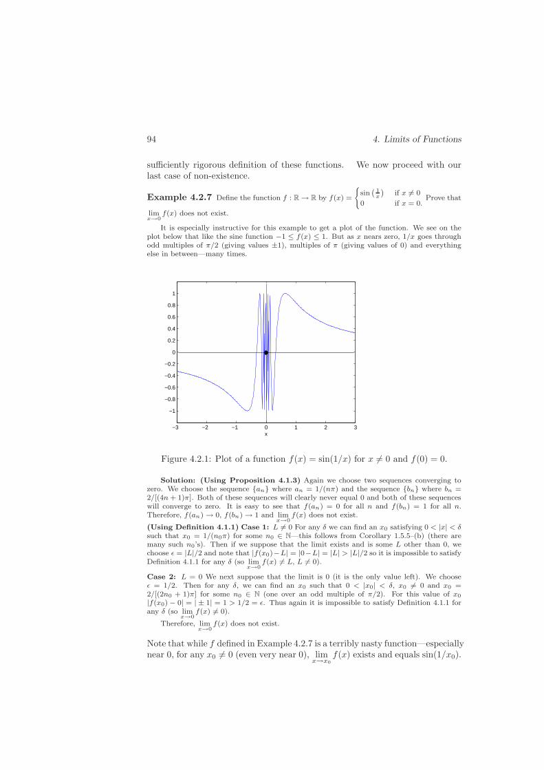
94 4. Limits of Functions
sufficiently rigorous definition of these functions. We now proceed with ourlast case of non-existence.
Example 4.2.7 Define the function f : R → R by f(x) =
{
sin(
1x
)
if x 6= 0
0 if x = 0.Prove that
limx→0
f(x) does not exist.
It is especially instructive for this example to get a plot of the function. We see on theplot below that like the sine function −1 ≤ f(x) ≤ 1. But as x nears zero, 1/x goes throughodd multiples of π/2 (giving values ±1), multiples of π (giving values of 0) and everythingelse in between—many times.
−3 −2 −1 0 1 2 3
−1
−0.8
−0.6
−0.4
−0.2
0
0.2
0.4
0.6
0.8
1
x
Figure 4.2.1: Plot of a function f(x) = sin(1/x) for x 6= 0 and f(0) = 0.
Solution: (Using Proposition 4.1.3) Again we choose two sequences converging tozero. We choose the sequence {an} where an = 1/(nπ) and the sequence {bn} where bn =2/[(4n + 1)π]. Both of these sequences will clearly never equal 0 and both of these sequenceswill converge to zero. It is easy to see that f(an) = 0 for all n and f(bn) = 1 for all n.Therefore, f(an) → 0, f(bn) → 1 and lim
x→0f(x) does not exist.
(Using Definition 4.1.1) Case 1: L 6= 0 For any δ we can find an x0 satisfying 0 < |x| < δsuch that x0 = 1/(n0π) for some n0 ∈ N—this follows from Corollary 1.5.5–(b) (there aremany such n0’s). Then if we suppose that the limit exists and is some L other than 0, wechoose ǫ = |L|/2 and note that |f(x0)−L| = |0−L| = |L| > |L|/2 so it is impossible to satisfyDefinition 4.1.1 for any δ (so lim
x→0f(x) 6= L, L 6= 0).
Case 2: L = 0 We next suppose that the limit is 0 (it is the only value left). We chooseǫ = 1/2. Then for any δ, we can find an x0 such that 0 < |x0| < δ, x0 6= 0 and x0 =2/[(2n0 + 1)π] for some n0 ∈ N (one over an odd multiple of π/2). For this value of x0
|f(x0) − 0| = | ± 1| = 1 > 1/2 = ǫ. Thus again it is impossible to satisfy Definition 4.1.1 forany δ (so lim
x→0f(x) 6= 0).
Therefore, limx→0
f(x) does not exist.
Note that while f defined in Example 4.2.7 is a terribly nasty function—especiallynear 0, for any x0 6= 0 (even very near 0), lim
x→x0
f(x) exists and equals sin(1/x0).

4.3 Limit Theorems 95
HW 4.2.1 (True or False and Why)(a) lim
x→0|x| = 0
(b) limx→−2
|x| = 2
(c) Suppose f : D → R, D ⊂ R, x0 ∈ R. If f(x0) is defined (x0 ∈ D), thenlimx→x0
f(x) = f(x0).
(d) limx→2
x2
2x− 5= −4
(e) Consider the function defined by f(x) =
1 x < 0
0 x = 0
−1 x > 0.
limx→0
f(x) = 0.
HW 4.2.2 Use the graphical approach to show that limx→3
2x+3 = 9. Specifically
find the δ1 and δ2 (of Figure 4.1.1), determine δ and show that it works. Explainwhy δ1 = δ2 in this example.
HW 4.2.3 (a) Prove that limx→4
7 = 7. Show this using the graphical approach
and then prove it twice—first using Definition 4.1.1 and then using Proposition4.1.3.(b) Prove that for any x0, c ∈ R, lim
x→x0
c = c.
HW 4.2.4 Define the function f : R → R by f(x) =
{
x2 + x+ 1 if x 6= 2
12 if x = 2.
Prove that limx→0
f(x) = 7—prove it twice, first using Definition 4.1.1 and then
using Proposition 4.1.3.
HW 4.2.5 Prove that limx→3
x2
x− 4= −9—prove it twice, first using Definition
4.1.1 and then using Proposition 4.1.3.
4.3 Limit Theorems
We don’t want to have to apply the Definition 4.1.1 or Proposition 4.1.3 everytime we have a limit. As was the case with sequential limits, we shall developlimit theorems that allow us to compute a large number of limits. You alreadyknow most of these limit theorems from your elementary calculus class. Ofcourse we will now include the proofs of these theorems. And it should notbe a surprise to you that the limit theorems will look very much like the limittheorems that we proved for limits of sequences. As with the proofs of conver-gence of the specific limits done in Section 4.2, parts (a), (b), (d) and (f) ofProposition 4.3.1 given below can be proved by either using the definition orProposition 4.1.3. Again we feel that you should see both approaches. For thatreason we will include both proofs for these parts. Since the proofs applyingDefinition 4.1.1 are very similar to the proofs of the analogous proofs for limits

96 4. Limits of Functions
of sequences and the proofs applying Proposition 4.1.3 are pretty easy, we willgive reasonably abbreviated versions of these proofs.
Proposition 4.3.1 Consider the functions f, g : D → R where D ⊂ R, supposethat c, x0 ∈ R and x0 is a limit point of D. Suppose lim
x→x0
f(x) = L1 and
limx→x0
g(x) = L2. We then have the following results.
(a) limx→x0
(f(x) + g(x)) = limx→x0
f(x) + limx→x0
g(x) = L1 + L2.
(b) limx→x0
cf(x) = c limx→x0
f(x) = cL1.
(c) There exists a δ3,K ∈ R such that for x ∈ D and 0 < |x − x0| < δ3,|f(x)| < K.
(d) limx→x0
f(x)g(x) =
(
limx→x0
f(x)
)(
limx→x0
g(x)
)
= L1L2.
(e) If L2 6= 0, then there exists a δ4,M ∈ R such that if x ∈ D and 0 < |x−x0| <δ4, then |g(x)| > M .(f) If L2 6= 0, then
limx→x0
f(x)
g(x)=
limx→x0f(x)
limx→x0g(x)
=L1
L2.
Proof: So that we don’t have to repeat it every time, throughout this prooflet {an} be any sequence such that an ∈ D for all n, an 6= x0 for any n, andan → x0.(a) (Using Definition 4.1.1) We suppose that we are given an ǫ > 0. Weapply the hypothesis lim
x→x0
f(x) = L1 with ǫ1 = ǫ/2 to get a
δ1 such that x ∈ D, 0 < |x− x0| < δ1 implies that |f(x) − L1| < ǫ1 = ǫ/2,
and the hypothesis limx→x0
g(x) = L2 with ǫ2 = ǫ/2 to get a
δ2 such that x ∈ D, 0 < |x− x0| < δ2 implies that |g(x) − L2| < ǫ2 = ǫ/2.
Then if we let δ = min{δ1, δ2} and require that x ∈ D and 0 < |x− x0| < δ, wehave
|(f(x) + g(x)) − (L1 + L2)| = |(f(x) − L1) + (g(x) − L2)|≤ |(f(x) − L1)| + |(g(x) − L2)| < ǫ/2 + ǫ/2 = ǫ.
Therefore limx→x0
(f(x) + g(x)) = L1 + L2.
(Using Proposition 4.1.3) We note that by Proposition 3.3.2–(a)
limn→∞
(f(an) + g(an)) = limn→∞
f(an) + limn→∞
g(an) = L1 + L2.
Since this holds true for any such sequence {an}, by Proposition 4.1.3 we getlimx→x0
(f(x) + g(x)) = L1 + L2.
4.3 Limit Theorems 97
(b) (Using Definition 4.1.1) If c 6= 0, we apply the hypothesis limx→x0
f(x) = L1
with ǫ1 = ǫ/|c|. Then setting δ = δ1 will give the desired result.If c = 0, the result is trivial since cf(x) = 0 for all x ∈ D—so it follows from
HW4.2.3-(b).
(Using Proposition 4.1.3) Since limn→∞
cf(an) = c limn→∞
f(an) by Proposition
3.3.2–(b), the result follows.
(c) (We do not give a proof of this result based on Proposition 4.1.3—it ispossible but it would not be very insightful.) Using the hypothesis lim
x→x0
= L1
with ǫ1 = 1, we get a δ3 such that if x ∈ D and 0 < |x − x0| < δ3 implies that|f(x)−L1| < ǫ1 = 1. Then by the backwards triangular inequality, Proposition1.5.8–(vi), we see that for all x such that x ∈ D and 0 < |x− x0| < δ3,
|f(x)| − |L1| ≤ |f(x) − L1| < 1,
or |f(x)| < 1 + |L1|. If we set K = 1 + |L1|, we are done.
(d) (Using Definition 4.1.1) We suppose that we given an ǫ > 0. We applythe hypothesis lim
x→x0
f(x) = L1 with ǫ1 = ǫ/(2L2) to get a
δ1 such that x ∈ D, 0 < |x = x0| < δ1 implies that |f(x) − L1| < ǫ1 = ǫ/(2L2),
and the hypothesis limx→x0
g(x) = L2 with ǫ2 = ǫ/(2K) to get a
δ2 such that x ∈ D, 0 < |x = x0| < δ2 implies that |g(x) − L2| < ǫ2 = ǫ/(2K).
We set δ = min{δ1, δ2, δ3} (where δ3 follows from part (c) of this proposition)and note that if x is such that x ∈ D and 0 < |x− x0| < δ (x satisfies all threerestrictions),
|f(x)g(x) − L1L2| = |f(x)(g(x) − L2) + L2(f(x) − L1)|≤ |f(x)||g(x) − L2| + |L2||f(x) − L1| < Kǫ2 + |L2|ǫ1.
Then using the fact that ǫ1 = ǫ/(2|L2|) and ǫ2 = ǫ/(2K), the result follows.Note that generally K 6= 0—or we can always choose it to be so. If L2 = 0,
the result follows by choosing ǫ2 = ǫ/K and δ = min{δ2, δ3}, and noting that
|f(x)g(x) − 0| = |f(x)||g(x)| < Kǫ2 = ǫ
whenever x ∈ D and 0 < |x− x0| < δ—we only use the hypothesis limx→x0
f(x) =
L1 to get K.
(Using Proposition 4.1.3) The result follows from Proposition 3.3.2–(d).
(e) (Again we do not include a proof of this result based on Proposition 4.1.3.)Since L2 is assumed to be nonzero, we use the hypothesis lim
x→x0
g(x) = L2
with ǫ2 = |L2|/2 and obtain a δ4 such that 0 < |x − x0| < δ4 implies that|g(x) − L2| < ǫ = |L2|/2. We have
|L2| − |g(x)| ≤ |L2 − g(x)| = |g(x) − L2| < ǫ = |L2|/2by the backwards triangular inequality, Proposition 1.5.8–(vi).

98 4. Limits of Functions
Thus when x ∈ D and 0 < |x − x0| < δ4, |g(x)| > |L2| − |L2|/2 = |L2|/2. If weset M = |L2|/2, we are done.
(f) (Using Definition 4.1.1) We suppose that we are given an ǫ > 0 and applythe hypotheses lim
x→x0
f(x) = L1 with respect to ǫ1 to get δ1 such that x ∈ D
and 0 < |x − x0| < δ1 implies |f(x) − L1| < ǫ1, limx→x0
g(x) = L2 with respect to
ǫ2 to get δ2 such that x ∈ D and 0 < |x − x0| < δ2 implies |g(x) − L2| < ǫ2,and L2 6= 0 and part (e) of this proposition to get δ4 such that x ∈ D and0 < |x − x0| < δ4 implies that g(x) > M . Then we set δ = min{δ1, δ2, δ4},require x to satisfy x ∈ D and 0 < |x− x0| < δ and note that
∣
∣
∣
∣
f(x)
g(x)− L1
L2
∣
∣
∣
∣
=
∣
∣
∣
∣
f(x)L2 − L1g(x)
L2g(x)
∣
∣
∣
∣
=
∣
∣
∣
∣
(f(x) − L1)L2 + L1(L2 − g(x))
L2g(x)
∣
∣
∣
∣
≤ |f(x) − L1||L2| + |L1||L2 − g(x)|g(x)|L2|
<ǫ1|L2| + |L1|ǫ2
M |L2|.
Thus we see that if we choose ǫ1 as ǫ1 = Mǫ/2 and ǫ2 as ǫ2 = M |L2|ǫ/(2|L1|,then
∣
∣
∣
∣
f(x)
g(x)− L1
L2
∣
∣
∣
∣
< ǫ and limx→x0
f(x)
g(x)=
L1
L2(if L1 = 0, the result follows by
choosing δ = min{δ1, δ4} and ǫ1 = ǫ/M).
(Using Proposition 4.1.3) Since by Proposition 3.4.1–(b)
limn→∞
f(an)
g(an)=
limn→∞ f(an)
limn→∞ g(an)=L1
L2
for any such sequence {an}, the result follows from Proposition 4.1.3.
Parts (a), (b), (d) and (f) of the above proposition are basic tools used inthe calculation of limits. However, to use these tools—which are always used tosimplify a given limit to a set of easier limits—we need some easier limits. Inthe next proposition we provide one of the easy limits that we need.
Proposition 4.3.2 (a) For any x0 ∈ R limx→x0
x = x0.
(b) Consider f1, · · · , fn : D → R where D ⊂ R, x0, L1, · · · , Ln ∈ R and x0
is a limit point of D. Suppose that limx→x0
fj(x) = Lj, j = 1, · · · , n. Then
limx→x0
f1(x) · f2(x) · · · fn(x) = L1 · L2 · · ·Ln.(c) Suppose x0 ∈ R and k ∈ N. Then lim
x→x0
xk = xk0 .
Proof: The proofs of these results are very easy. Result (a) follows by choosingδ = ǫ in Definition 4.1.1. Property (b) is an elementary application of math-ematical induction using part (d) of Proposition 4.3.1. And then the resultgiven in part (c) follows from parts (a) and (b) of this proposition (or by applyProposition 4.3.1–(d) k − 1 times along with part (a) of this proposition).
We next include an inductive version of Proposition 4.3.1–(a) and use thisresult—along with the other parts of Proposition 4.3.1 to compute a large class oflimits. Let p and q denote mth and nth degree polynomials, respectively, p(x) =a0x
m+a1xm−1 + · · ·+am−1x+am and q(x) = b0x
n+b1xn−1 + · · ·+bn−1x+an.

4.3 Limit Theorems 99
Proposition 4.3.3 (a) Consider f1, · · · , fn : D → R where D ⊂ R, x0, L1, · · · , Ln ∈R and x0 is a limit point of D. Suppose that lim
x→x0
fj(x) = Lj, j = 1, · · · , n.Then lim
x→x0
(f1(x) + f2(x) + · · · + fn(x)) = L1 + L2 + · · · + Ln.
(b) For all x0 ∈ R limx→x0
p(x) = p(x0) = a0xm0 + a1x
m−10 + · · · + am−1x0 + am.
(c) If x0 ∈ R and q(x0) 6= 0, then
limx→x0
p(x)
q(x)=p(x0)
q(x0)=a0x
m0 + a1x
m−10 + · · · + am−1x0 + am
b0xn0 + b1xn−10 + · · · + bn−1x0 + bn
.
Proof: As was the case with Proposition 4.3.2 the proof of this propositionis also very easy. Part (a) can be proved by applying mathematical inductionalong with part (a) of Proposition 4.3.1. The result given in part (b) thenfollows from part (a) of this result, Proposition 4.3.1–(b) and Proposition 4.3.2–(c). And finally, to prove part (c) we apply the quotient rule from Proposition4.3.1–(f) along with part (b) of this proposition.
We are now able to compute a large class of limits. We have intentionallyskipped functions involving irrational exponents and functions of the form ax
(which are two other very basic ”easy limits” that we use along with Propo-sition 4.3.1 to compute limits) because we will give a rigorous mathematicalintroduction to these functions in Chapter 5 and 6—so discussiing their limitsat this time would be cheating. If we returned to the examples considered inSection 4.2 we would now be able to compute the limits considered in Examples4.2.1–4.2.3 very easily. To compute a limit such as that considered in Example4.2.4, we proceed much the way we did in our elementary course and computeas follows.
limx→2
x4 − 16
x− 2= lim
x→2
(x− 2)(x+ 2)(x2 + 4)
x− 2
= limx→2
(x+ 2)(x2 + 4) because we know that x− 2 6= 0
= 32 by Proposition 4.3.3–(b).
Before we leave this section we include one more limit result—the Theorem,analogous to the sequential Sandwich Theorem, Proposition 3.4.2.
Proposition 4.3.4 Consider the functions f, g, h : D → R where D ⊂ R,suppose that x0 ∈ R and x0 is a limit point of D. Suppose lim
x→x0
f(x) =
limx→x0
g(x) = L and there exists a δ1 such that f(x) ≤ h(x) ≤ g(x) for x ∈ D
and 0 < |x− x0| < δ1. Then limx→x0
h(x) = L.
Proof: Suppose ǫ > 0 is given. Let δ2 and δ3 be such that 0 < |x − x0| < δ2implies |f(x) − L| < ǫ or L − ǫ < f(x) < L + ǫ, and 0 < |x − x0| < δ3 implies|g(x) − L| < ǫ or L − ǫ < g(x) < L + ǫ. Let δ = min{δ1, δ2, δ3} (Define δ) andsuppose that x satisfies x ∈ D and 0 < |x− x0| < δ. Then
L− ǫ < f(x) ≤ h(x) ≤ g(x) < L+ ǫ,

100 4. Limits of Functions
or L−ǫ < h(x) < L+ǫ (Step 2: δ works). Thus |h(x)−L| < ǫ so limx→x0h(x) =
L.
HW 4.3.1 (True and False and why) (a) Suppose f : D → R, D ⊂ R, x0, L ∈R, x0 is a limit point of D and lim
x→x0
f(x) = L. Then limx→x0
|f(x)| = |L|.(b) Suppose f : D → R, D ⊂ R, x0, L ∈ R, x0 is a limit point of D, lim
x→x0
f(x) =
L and L > 0. Then there exists a neighborhood of x0, N(x0), such that f(x) > 0for all x ∈ N(x0).(c) Consider f, g : D → R, D ⊂ R, x0 ∈ R and x0 is a limit point of D. Supposefurther that lim
x→x0
(f(x) + g(x)) and limx→x0
g(x) exist. Then limx→x0
f(x) exists.
(d) Suppose f : D → R, D ⊂ R, x0 ∈ R and x0 is a limit point of D. Supposefurther that lim
x→x0
f(x) exists and there exists a punctured neighborhood of x0,
N̂δ(x0), such that f(x) > 0 for x ∈ N̂δ(x0). It may be the case that limx→x0
f(x) =
0.(e) Suppose f, g, h : D → R, D ⊂ R, x0 ∈ R and x0 is a limit point of D.Suppose also that lim
x→x0
f(x) = limx→x0
g(x) = L and there exists a δ such that
f(x) < h(x) < g(x) for x satisfying 0 < |x − x0| < δ. In this situation it is notnecessarily the case that lim
x→x0
h(x) = L.
HW 4.3.2 Prove that limx→2
x− 2√x−
√2
= 2√
2.
HW 4.3.3 Suppose f, g : D → R, D ⊂ R, x0 ∈ R and x0 is a limit point ofD. Suppose further that f(x) ≤ g(x) on some punctured neighborhood of x0,N̂δ(x0), and both limits lim
x→x0
f(x) and limx→x0
g(x) exist. Prove that limx→x0
f(x) ≤limx→x0
g(x).
4.4 Limits at Infinity, Infinite Limits and One-
sided Limits
Limits at Infinity For all of the limits consider so far in this chapter bothx0 and L must be real. In this section we want to introduce limits where x0
and or L are ±∞. Of course we need definitions to extend the limit conceptsto these situations. If you think about it a bit, you should realize that we willwant lim
x→∞f(x) to be very much like the sequential limit—except the definition
will now have to allow for x values in some interval (N,∞) rather than thediscrete points of N. Note that for convenience we define the limits at infinitefor functions defined on intervals such as (−∞, a) or (a,∞) for some a. Wecould give these definitions for domains less than these intervals but we wouldhave to fix up the domains so that we guaranteed that ±∞ was a limit pointof D—which we haven’t and don’t really want to define. We begin with thefollowing definition.

4.4 Infinite and One-sided Limits 101
Definition 4.4.1 For f : (a,∞) → R for some a ∈ R and L ∈ R, we say thatlimx→∞
f(x) = L if for every ǫ > 0 there exists an N ∈ R such that x > N implies
that |f(x) − L| < ǫ.Likewise, if f is defined on (−∞, a) for some a, lim
x→−∞f(x) = L if for every
ǫ > 0 there exists an N ∈ R such that x < N implies that |f(x) − L| < ǫ.
You probably computed some limits of this sort in your basic calculus class.One of the common applications of limits at ±∞ is to determine asymptotesto curves. Methods for computing limits at infinity are similar to the methodsfor computing sequential limits. For example, the approach used to calculate a
limit such as limx→∞
2x2 + x− 3
3x2 + 3x+ 3is to perform the following computation.
limx→∞
2x2 + x− 3
3x2 + 3x+ 3= lim
x→∞2 + 1/x− 3/x2
3 + 3/x+ 3/x2=
limx→∞ 2 + 1/x− 3/x2
limx→∞ 3 + 3/x+ 3/x2=
2
3.
(Compare this result with the limit evaluated at the beginning of Section 3.4.)To perform the above computation we first multiplied the numerator and de-nominator by 1/x2 and then used ”limit of a quotient is the quotient of thelimits”, ”limit of a sum is the sum of the limits”, ”limit of a constant times afunction is the constant times the limit”, ”limit of a constant is that constant”and ”the limit of 1/xk as x goes to infinity is zero” (k ∈ N). Clearly, at presentwe do not have these results, and hopefully equally clearly, these results arecompletely analogous to the results proved for sequences in Propositions 3.3.2,3.4.1, Example 3.3.1 and HW3.2.1-(b). We include these results in the followingtwo propositions.
Proposition 4.4.2 Suppose that f, g : (a,∞) → R, for some a ∈ R, limx→∞
f(x) =
L1, limx→∞
g(x) = L2 and c ∈ R. We have the following results.
(a) limx→∞
(f(x) + g(x)) = L1 + L2.
(b) limx→∞
cf(x) = c limx→∞
f(x) = cL1.
(c) There exists an N,K ∈ R such that for x ∈ (a,∞) and x > N , |f(x)| ≤ K.(d) lim
x→∞f(x)g(x) = L1L2.
(e) If L2 6= 0 then there exists an N,M ∈ R such that |g(x)| ≥M for all x > N .
(f) If L2 6= 0, then limx→∞
f(x)
g(x)=L1
L2.
Proposition 4.4.3 (a) For c ∈ R limx→∞
c = c.
(b) limx→∞
(1/x) = 0
(c) For k ∈ N limx→∞
(1/xk) = 0.
We are not going to prove these two propositions. Their proofs are justcopies of the analogous sequential results. Likewise, we could also take some

102 4. Limits of Functions
particular examples such as limx→∞
2x+ 3
5x+ 7=
2
5and use Definition 4.4.1 to prove
this statement. We will not do that because such a proof would be almostidentical to the proof given in Example 3.2.3 (when we did the analogous resultfor sequences). Also we should add that there are versions of Propositions 4.4.2and 4.4.3 for the case when x approaches −∞. And finally note that we havenot mentioned a result analogous to Example 3.5.1. It is possible to prove thatfor 0 < c < 1, lim
x→∞cx = 0. However, since we will wait until Chapter 6 to define
cx, we do not consider this limit at this time.Infinite Limits In Example 4.2.5 we showed that lim
x→0(1/x2) does not exist. We
mentioned as a part of the proof that the limit wanted to go to infinity—so sinceaccording to Definition 4.1.1 it is necessary that L ∈ R, the limit cannot exist.We want to be able to show that the limit above does not exist in a much nicerway than the nonexistence of the limits considered in Examples 4.2.6 and 4.2.7.Just as we included an alternative definition for sequences converging to infinityin Section 3.6, we want the same concept for limits of functions. Consider thefollowing definition.
Definition 4.4.4 (a) Suppose that f : D → R, D,R ⊂ R, x0 ∈ R and x0 alimit point of D. We say that lim
x→x0
f(x) = ∞ if for every M > 0 there exists a
δ such that x ∈ D, 0 < |x− x0| < δ implies that f(x) > M .(b) lim
x→x0
f(x) = −∞ if for every M < 0 there exists an δ such that x ∈ D,
0 < |x− x0| < δ implies that f(x) < M .
We now return to the consideration of the example given in Example 4.2.5.
Example 4.4.1 Prove that limx→0
(1/x2) = ∞.
Solution: We suppose that we are given an M > 0. We must find a δ so that 0 < |x− 0| < δimplies that f(x) > M , i.e. we need 1
x2 > M . This last inequality is equivalent to x2 < 1/M .
This inequality is satisfied if |x| < 1/√
M . Thus we define δ = 1/√
M (Step 1: Define δ) andsuppose that 0 < |x| < δ = 1/
√M . Then for x 6= 0, |x|2 = x2 < 1/M and 1/x2 > M which is
what we had to prove (Step 2: δ works). Therefore limx→0
1/x2 = ∞.
Note that we did not consider x = 0 at all. This is a place where the part of therequirement ”0 <” is important.
If we wanted to, we could now prove some theorems pertaining to infinitelimits. This surely would be overkill. However, we should be aware that it ispossible to obtain all of the results analogous to those in Proposition 3.6.2. Andfinally, we should realize that we could also define infinite limits as x approacheseither positive or negative infinity, i.e. lim
x→−∞(x2 + 1) = ∞. Hopefully you
are now capable of piecing the definitions given above to obtain the necessarydefinition for such limits—if they are needed. Limits such as this last one arenot common.
One-sided Limits If you feel that this topic does not fit particularly well withthe other two topics in the section, you are right—we had to find a place toput it. Quite literally there are times when instead of approaching the limiting
4.4 Infinite and One-sided Limits 103
point from either side, we want to only consider points to the right or left ofx0. We did this when we considered limits at ±∞ but in that case there wereno points ”on the other side.” We have three easy approaches to this idea—weshall do all three.
We begin by considering f : D → R where D ⊂ R and x0 ∈ R (where wealways keep in mind the most common case where D = [a, b]). We define twonew functions f+ : D+ → R where D+ = D ∩ (x0,∞) and f− : D− → R whereD− = D ∩ (−∞, x0). We make the following definition.
Definition 4.4.5 (a) If x0 is a limit point of D+, we define limx→x0+
f(x) =
limx→x0
f+(x).
We refer to this limit as the limit of f as x approaches x0 from the right or theright hand limit of f at x0.(b) If x0 is a limit point of D−, we define lim
x→x0−f(x) = lim
x→x0
f−(x).
We refer to this limit as the limit of f as x approaches x0 from the left or theleft hand limit of f at x0.
We should note that the functions f+ and f− are just copies of f to the rightand the left of x0, respectively—hence using f+ and f− we get the right and lefthand limits of f , respectively. The fact that Definition 4.1.1 is a very generaldefinition of a limit allows us to easily define the right and left hand limits. Alsonotice that it is still a requirement that x0 is a limit point of D+ and D−—thisis to guarantee that we have enough points of D on either side of x0 to allow usto apply Definition 4.1.1. Note that if x0 is a limit point of either D+ or D−,then x0 will also be a limit point of D.
Before we look at some results concerning right and left hand limits, weinclude the more common definition in the following result.
Proposition 4.4.6 Suppose that f : D → R where D ⊂ R and x0, L ∈ R.(a) Suppose that x0 is a limit point of D ∩ (x0,∞). Then lim
x→x0+f(x) = L if
and only if for every ǫ > 0 there exists a δ such that x ∈ D and 0 < x− x0 < δimplies that |f(x) − L| < ǫ.(b) Suppose that x0 is a limit point of D ∩ (−∞, x0). Then lim
x→x0−f(x) = L if
and only if for every ǫ > 0 there exists a δ such that x ∈ D and 0 < x0 − x < δimplies that |f(x) − L| < ǫ.
Proof: (a) (⇒) We begin by assuming that limx→x0+
f(x) = L, i.e. limx→x0
f+(x) =
L. This means that for every ǫ > 0 there exists a δ such that x ∈ D+ and 0 <|x−x0| < δ implies that |f+(x)−L| < ǫ. We note that if x ∈ D+ = D∩(x0,∞),then |x−x0| = x−x0, so 0 < |x−x0| < δ is equivalent to 0 < x−x0 < δ. Also,note that if x ∈ D+, then x ∈ D also. And finally, for x ∈ D+ f+(x) = f(x).Thus for the δ given we see that x ∈ D and 0 < |x − x0| = x − x0 < δ implies|f(x) − L| < ǫ.
(⇐) We will skip the proof of this direction because it is so similar to the proofgiven for part (b)
104 4. Limits of Functions
(b) (⇒) We will skip the proof of this direction because it is so similar to theproof given for part (a).
(⇐) We suppose that for every ǫ > 0 there exists a δ so that if x ∈ D and0 < x0 − x < δ implies |f(x) − L| < ǫ. Note that x ∈ D and 0 < x0 − x < δ isequivalent to x ∈ D− and |x− x0| < δ. Also, if x ∈ D and 0 < x0 − x < δ, thenf(x) = f−(x). Thus for x ∈ D− and 0 < x0 − x < δ we have |f−(x) − L| < ǫor lim
x→x0
f−(x) = L or limx→x0−
f(x) = L.
The way that we apply Proposition 4.4.6 in a one-sided limit proof is verysimilar to the way that we applied Definition 4.1.1—except that we now onlyneed to consider points on one side of x0.
The third characterization of one-sided limits should be very familiar to us.In Proposition 4.1.3 we gave a sequential characterization of limits—we can dothe same thing for one-sided limits. We state the following proposition.
Proposition 4.4.7 Suppose that f : D → R, D ⊂ R, x0, L ∈ R.(a) Suppose that x0 is a limit point of D ∩ (x0,∞). Then lim
x→x0+f(x) = L if
and only if for any sequence {an} such that an ∈ D for all n, an > x0 for alln, and lim
n→∞an = x0, then lim
n→∞f(an) = L.
(b) Suppose that x0 is a limit point of D ∩ (−∞, x0). Then limx→x0−
f(x) = L if
and only if for any sequence {an} such that an ∈ D for all n, an < x0 for alln, and lim
n→∞an = x0, then lim
n→∞f(an) = L.
Proof: We will skip this proof because it is so much like the proof of Proposition4.1.3. For the (⇒) direction of part (a) for a given ǫ > 0 the right hand limithypothesis gives a δ, this δ used as the ”ǫ” in the assumption that an → x0
(and it works because we have assumed that an > 0) gives an N which is theN that we need to prove that f(an) → L as n→ ∞. The (⇒) direction of part(b) is essentially the same.
To prove the (⇐) directions we again assume false and use this assumptionto create a sequence {an} that contradicts our hypthesis—because the one-sidedlimit is used the our contradiction assumption, the sequence will either greaterthan or less than x0.
We emphasize that when we want to prove things about one-sided limits,we will generally use Propositions 4.4.6 and 4.4.7. We gave Definition 4.4.5as we did to emphasize the ”one sidedness” of the functions when we considerone-sided limits.
In Example 4.2.2 we proved that limx→2
x2 = 4. It is very easy to show that
limx→2+
x2 = 4 and limx→2−
x2 = 4. If we use Proposition 4.4.6 we can choose
δ = min{1, ǫ/5} (the same δ used in Example 4.2.2). If we apply Proposition4.4.7 to prove that lim
x→2+x2 = 4, we use a sequence an → 2 with an > 2 and
the fact that limn→∞
a2n =
(
limn→∞
an
)(
limn→∞
an
)
= 2 · 2 = 4. And of course the
application of Proposition 4.4.7 to limx→2−
x2 is similar except that this time we

4.4 Infinite and One-sided Limits 105
assume that the sequence satisfies an < 2. We do not try to apply Definition4.4.5—either Propositions 4.4.6 and 4.4.7 are much cleaner ways to prove one-sided limits.
If f(x) =
{
1 if x ≥ 0
0 if x < 0,we showed in Example 4.2.6 that lim
x→0f(x) does not
exist. It is very easy to show that limx→0+
f(x) = 1 and limx→0−
f(x) = 0. If we
were to apply Proposition 4.4.6, we can choose δ = 1 (or anything else) for bothof them. If we apply Proposition 4.4.7, the results follow because f(an) = 1 ifan > 0 and f(an) = 0 if an < 0.
In Example 4.2.7 we showed that limx→0
f(x) does not exist when f(x) ={
sin(1/x) x 6= 0
0 x = 0.The easiest way to show that lim
x→0+f(x) does not exist is
to use Proposition 4.4.6 with two different sequences an = 1/nπ and bn =2/(4n+1)π—where just as we did in Example 4.2.7 we find that f(an) → 0 andf(bn) → 1. To show that lim
x→0−f(x) does not exist we again apply Proposition
4.4.6, this time with the sequences {−an} and {−bn}. The fact that theseone-sided limits do not exist should be clear by looking at Figure 4.2.1.
We do not define one-sided infinite limits but we should be clear that thereare such limits (and we will not define them here). In Example 4.2.5 we showed
in limx→0
1
x2does not exist in R, and then in Example 4.4.1 we showed that
limx→0
1
x2= ∞. If we are given M > 0 and choose δ = 1/
√M—-just as we did
in Example 4.4.1, we can show that 0 < x < δ = 1/√M implies that 1
x2 > M .
Thus limx→0+
1
x2= ∞. The same δ can be used to prove that lim
x→0−1
x2= ∞ also.
The limit limx→0
1
xis slightly different. This limit does not exist either by
Definition 4.1.1 (i.e. not in R) and not by Definition 4.4.4. However it should
be clear that limx→0+
1
x= ∞ and lim
x→0−1
x= −∞. Proof of the right hand limit is as
follows. Suppose M > 0 is given. Choose δ = 1/M . Then if 0 < x < δ = 1/M ,∣
∣
1x
∣
∣ = 1x > M . Therefore lim
x→0+
1
x= ∞. The proof of the left hand limit is
similar.Before we leave this topic we want to include one important result. We
notice that when we considered the left and right hand limits of f(x) = x2 atx0 = 2, we got 4—they same value as lim
x→2x2. When we considered the functions
f(x) =
{
1 if x ≥ 0
0 if x < 0and f(x) =
{
sin(1/x) x 6= 0
0 x = 0,
for both of which the limit limx→0
f(x) did not exist, we see that in one case both
one-sided limits exist but are different and in the other case neither of the one-sided limits exist. These examples pretty much illustrate all possibilities of thefollowing theorem.

106 4. Limits of Functions
Proposition 4.4.8 Consider the function f : D → R where D,R ⊂ R, supposethat L, x0 ∈ R and x0 is a limit point of both D ∩ (x0,∞) and D ∩ (−∞, x0).Then lim
x→x0
f(x) exists if and only if both limx→x0+
f(x) and limx→x0−
f(x) exist and
are equal.
Proof: (⇒) We assume that limx→x0
f(x) exists, i.e. for every ǫ > 0 there exists
a δ such that x ∈ D and 0 < |x − x0| < δ implies that |f(x) − L| < ǫ for someL ∈ R. Note that 0 < |x−x0| < δ implies that 0 < x−x0 < δ or 0 < x0−x < δ.Thus x0 is a limit point of D ∩ (x0,∞) and we have a δ such that
x ∈ D and 0 < x− x0 < δ implies that |f(x) − L| < ǫ
thus by Proposition 4.4.6-(a) limx→x0+
f(x) = L
and x0 is a limit point of D ∩ (−∞, x0) and we have a δ such that
x ∈ D and 0 < x0 − x < δ implies that |f(x) − L| < ǫ
thus by Proposition 4.4.6-(b) limx→x0−
f(x) = L,
which is what we were to prove.
(⇐) Suppose ǫ > 0 is given. We suppose that limx→x0+
f(x) = L and limx→x0−
f(x) =
L. Then there exists a δ1 and δ2 such that if x satisfies either 0 < x− x0 < δ1or 0 < x0 − x < δ2 implies that |f(x) − L| < ǫ. Let δ = min{δ1, δ2} (Step 1:Define δ). The if x satisfies 0 < |x − x0| < δ, x satisfies 0 < x − x0 < δ or0 < x0 − x < δ. So x satifies 0 < x− x0 < δ ≤ δ1 or 0 < x0 − x < δ ≤ δ2. Thus|f(x) − L| < ǫ (Step 2: δ works), so lim
x→∞f(x) = L.
There are times when we want to prove a particular limit that the abovetheorem is very useful. We can handle the function on each side of x0 separately,get the same one-sided limits and hence prove our limit result.
HW 4.4.1 (True or False and why) (a) If x0 is a limit point of D ⊂ R, thenx0 is a limit point of D+ = D ∩ (x0,∞) and D− = D ∩ (−∞, x0).(b) Suppose f : [0, 1) → R and that lim
x→1−f(x) exists. Then lim
x→1+f(x) exists
also.(c) Suppose f : [0, 1] → R and that lim
x→1−f(x) exists. Then lim
x→1+f(x) exists
also.(d) Suppose f : [0, 1) → R and that lim
x→1−f(x) exists. Then lim
x→1f(x) exists.
(e) Suppose that f(x) = 1/x4 and g(x) = x. We know that limx→0
f(x) = ∞ and
limx→0
g(x) = 0. Then limx→0
f(x)g(x) = 0 · ∞ = 0.
HW 4.4.2 (a) Prove that limx→0
1/x4 = ∞. (b) Prove that limx→∞
1/x4 = 0.
(c) Prove that limx→∞
sinx does not exist. (d) Prove that limx→∞
x
2x− 1− 1
2.
Chapter 5
Continuity
5.1 An Introduction to Continuity
In the preceeding chapters we have been building basics and tools. In thischapter we introduce the concept of a continuous function and results relatedto continuous functions. The class of continuous functions is a very importantset of functions in many areas of mathematics. Also there are a lot of very niceand useful properties of continuous functions. We begin with the definition ofcontinuity.
Definition 5.1.1 Consider a function f : D → R where D ⊂ R and a pointx0 ∈ D. The function f is continuous at x0 if for every ǫ > 0 there exists a δsuch that for x ∈ D and |x− x0| < δ, then |f(x) − f(x0)| < ǫ.If the function f is continuous at x for all x ∈ D, then f is said to be continuouson D.If the function f is not continuous at a point x = x0, then f is said to bediscontinuous at x = x0.
In the last chapter we studied what it meant for a function to have a limit at apoint. Often the definition of continuity is given in terms of limits—especiallyin the elementary calculus texts. We state the following proposition.
Proposition 5.1.2 Consider a function f : D → R where D ⊂ R and a pointx0 ∈ D. Suppose that x0 is a limit point of the set D. If lim
x→x0
f(x) = f(x0),
then the function f is continuous at x = x0.If x0 ∈ D and x0 is a limit point of D but lim
x→x0
f(x) does not exist, or exists
but does not equal f(x0), then f is not continuous at x = x0.
Proof: This proof is very easy. Let ǫ > 0 be given. If we apply the definitionof lim
x→x0
f(x) = f(x0) we get a δ such that 0 < |x − x0| < δ implies that
|f(x) − f(x0)| < ǫ. But this is almost what we need to satisfy Definition 5.1.1.We need to get rid of the ”0 <” requirement. But when x = x0, we know that
107

108 5. Continuity
|f(x) − f(x0)| = 0 < ǫ so the ”0 <” part of the restriction on x is completelyunnecessary. Therefore f is continuous at x = x0.
If x0 ∈ D is a limit point of D and it is not the case that limx→x0
f(x) = f(x0)
(either the limit does not exist or it exists but equals something other thanf(x0)), then there is some ǫ so that for any δ, there is an xδ ∈ D such that0 < |x − xδ| < δ and |f(xδ) − f(x0)| ≥ ǫ. This also negates Definition 5.1.1 sof is not continuous at x = x0.
We want to emphasize that this result is not an ”if and only if” result, i.e.this does not provide us with a statement that is equivalent to the definitionof continuity. However, some texts use this as their definition—usually onlybasic calculus texts. The function that we considered in HW4.1.1 shows thathypotheses given in Proposition 5.1.2 are not equivalent to Definition 5.1.1.In HW4.1.1–(a) we considered the domain D = [0, 1] ∪ {2} and the functionf : D → R, f(x) = x2. The True-False question was whether lim
x→2f(x) exists
and equals 4. Of course the answer is False because for that limit to exist,2 must be a limit point of D. However, f is continuous at x = 2—if we setδ = 1/2, Definition 5.1.1 is satisfied. It is not a requirement for continuity atx = x0 that lim
x→x0
f(x) exist. A function will be continuous at isolated
points of its domain—the limit of the function will not exist at those points.This is not a terribly important distinction for our work. Let us emphasize thatProposition 5.1.2 can be used to prove continuity at points of the domain thatare limit points of the domain—which in this level of a text is most of them.
In Example 4.2.1 we showed that limx→3
2x + 3 = 9. If we set f1(x) = 2x+ 3
and choose the domain to be R (a reasonable domain for that function), wenote that f1 is defined at x = 3 and f1(3) = 9. Thus by Proposition 5.1.2the function f1 is continuous at x = 3. It would be equally easy to mimicthe work done in Example 4.2.1, (omitting the ”0 <” part) to show that f1satisfies Definition 5.1.1 at x = 3. (Choose δ = ǫ/2. Then for |x − 3| < δ,|f1(x)− 9| = |(2x+ 3)− 9| = 2|x− 3| < 2δ = ǫ.) It is equally easy to see—usingeither Definition 5.1.1 or Proposition 5.1.2 (or we could use Proposition 4.3.3-(b) along with Proposition 5.1.2—that the function f1 is continuous at x = x0
for any x0 ∈ R. Thus f1 is continuous on R.Likewise, we showed in Example 4.2.2 that the function f2(x) = x2 is con-
tinuous at x = 2 (given that we define f2 on some reasonable domain such asD = R) and in Example 4.2.3 the function f3(x) = x−2
x+3 is continuous at x = −2.Note that in the case of the function f3, the largest (most logical) domain thatwe can choose is the set D3 = {x : x ∈ R and x 6= −3}. Recall that in the workdone in Examples 4.2.1–4.2.3, the ”0 <” part of the definition of a limit was notrelevant. We noted that in each case |f(x) − L| < ǫ when x = x0 also—in factin each of these cases |f(x) − L| = 0 when x = x0. This is exactly why f1, f2and f3 are continuous at x = 3, x = 2 and x = −2, respectively.
If we consider f2 and f3 at arbitrary points of D2 and D3, respectively, wecan use either Definition 5.1.1, or Proposition 4.3.3 and Proposition 5.1.2 toshow that f2 is continuous on D2 and f3 is continuous on D3. Hopefully it is

5.1 Introduction 109
obvious that f3 is not continuous at x = −3. A function cannot be continuousat a point that is not in the domain of the function.
In Example 4.2.4 we showed that limx→4
x3 − 64
x− 4= 48. However, if we define
f4(x) =x3 − 64
x− 4and allow the domain to be what is sort of f4’s natural domain,
D4 = {x : x ∈ R and x 6= 4}, then f4 is surely not continuous at x = 4 sincef4 is not defined at x = 4. If we were to define a new function f8 so thatf8(x) = f4(x) for all x ∈ R, x 6= 4 and define f8(4) = 48, then the domain of f8would be D8 = R, f8 will be continuous at x = 4 and f8 would be continuouson all of R—use Proposition 5.1.2.
And finally we showed in Examples 4.2.5, 4.2.6 and 4.2.7 that the functions
f5(x) = 1/x2, f6(x) =
{
1 if x ≥ 0
0 if x < 0,and f7(x) =
{
sin(
1x
)
if x 6= 0
0 if x = 0
are not continuous at x = 0. This can be seen by the last part of Proposition5.1.2 because 0 is a limit point of the domain of each of these domains and thelimit as x approaches 0 of each of these functions does not exist. In the case off5 it is even easier yet. If a function isn’t defined at a particular point, there isno way that the function can be continuous at that point.
A Graphical Example In Figure 5.1.1 we plot a function where the domainis assumed to be approximately the set above which there is a graph plotted(except for the points xE and xF at which the function f is not defined. Wemake the following claims.
xA xFxExDxCxB
Figure 5.1.1: Plot of a function continuous at xA, discontinuous at xB–xF . Asmall open circle denotes a point at which the function is not defined. A smallfilled circle denotes one point of definition.
• At point xA, though the graph has a ”corner” at that point, the functionis continuous at that point. (Generally, a function is continuous at well-defined corners.)

110 5. Continuity
• At point xB, the function is defined at x = xB but will not be continuousat xB . Though lim
x→xB
f(x) exists, there is no way that limx→xB
f(x) will equal
f(xB). When x is near xB, f(x) is not near f(xB).
• The function is not continuous at points xC , xD and xE . These points aresimilar to the point x = 0 considered in Example 4.2.6 and the proof thatthe limit does not exist at points xC and xD would be very similar to theargument used in Example 4.2.6. We wanted to emphasize that each ofthese points represent a jump in the function. The points xC and xD arepoints where the function is defined on the left and right side of the jump,respectively. At the point xE the function is not continuous because it hasa jump at that point and it is not defined at the jump point. A functioncannot be continuous at a point at which it is not defined.
• The function is not continuous at point xF . Even though the function isnicely behaved on both sides of the point xF , the function must be definedat a point to be continuous at that point. Note that lim
x→xF
f(x) exists, and
if we were to define f at the point xF to be limx→xF
f(x), then the function
f would be continuous at x = xF .
Before we leave this section we include one of the basic continuity theorems.We see that this result is the continuity analog to the limit result, Proposition4.1.3.
Proposition 5.1.3 Suppose that f : D → R, D,R ⊂ R and x0 ∈ R and x0.Then f is continuous at x = x0 if and only if for any sequence {an} such thatan ∈ D for all n and lim
n→∞an = x0, then lim
n→∞f(an) = f(x0).
Proof: Before we begin let’s look at some of the difference between the abovestatement and that given in Proposition 4.1.3. Because we now assume thatx0 ∈ D and because we no longer have the ”0 <” restriction on the range ofx, we now do not require that an 6= x0. In addition, in the above propositionstatement we no longer require that x0 in a limit point of D. We know thatwhen we consider the continuity of a function, it is permissible to have isolatedpoints in D and the function will always be continuous at those isolated points.Despite these differences the proof of this result is essentially identical to thatof Proposition 4.1.3.
(⇒) We are assuming that f is continuous at x0 ∈ D. We consider any sequence{an} where an ∈ D and an → x0. We suppose that we are given an ǫ > 0. Thecontinuity of f at x = x0 implies that there exists a δ such that |x − x0| < δimplies that |f(x) − f(x0)| < ǫ. If we apply the definition of the fact thatan → x0 with the traditional ”ǫ” replaced by δ, we get an N such that n > Nimplies that |an − x0| < δ. Then the continuity of f statement implies that forn > N , |f(an) − f(x0)| < ǫ. Thus f(an) → f(x0).
(⇐) We suppose that f is not continuous at x0, i.e. for some ǫ0 > 0 for any δthere exists an xδ ∈ D such that |xδ − x0| < δ and |f(xδ) − f(x0)| ≥ ǫ.

5.2 Examples 111
Let δ = 1 so we get an x1 ∈ D such that |x1 − x0| < 1 and |f(x1) − f(x0)| ≥ ǫ.
Let δ = 1/2 so we get an x2 ∈ D such that |x2−x0| < 1/2 and |f(x2)−f(x0)| ≥ ǫ.
And in general
let δ = 1/n so we get an xn ∈ D such that |xn−x0| < 1/n and |f(xn)−f(x0)| ≥ǫ.
Thus we have a sequence {xn} such that xn → x0 and f(xn) 6→ f(x0). Thisis a contradiction so f is continuous at x = x0.
We should be mildly concerned that the proof of Propositions 4.1.3 and 5.1.3are the same—we pointed out the differences between the two results. The factthat we no longer require that an 6= x0 is no problem because f is now definedat x0 and the restriction 0 < |x − x0| < δ is replaced by |x− x0| < δ. The factthat we do not require that x0 be a limit point of D is taken care of by thefact that if x0 is an isolated point of D (not a limit point) we can consider thesequence {x0, x0, x0, · · · }—in fact the tail end of all of the sequences containedin D that converges to x0 look like this if x0 is an isolated point of D.
There are some texts that use the right hand side of Proposition 5.1.3 asthe definition of continuity—since the proposition is an ”if and only if” result,this is completely permissible. The definition of continuity given in Definition5.1.1 is the most common definition. Of course there are many times that thesequential characterization of continuity is very useful. We feel that you mustbe comfortable with using both Definition 5.1.1 and Proposition 5.1.3 (just aswe tried to force you to work with both Definition 4.1.1 and Proposition 4.1.3).Specifically, as was the case with limits, when we want to show that a function isnot continuous at a given point, it is usually easier to apply Proposition 5.1.3—providing either one sequence {an} at which {f(an)} does not converge, or twosequences {an} and {bn} for which {f(an)} and {f(bn)} converge to differentvalues. When a push comes to a shove, we will use which ever characterizationis best at the time.
HW 5.1.1 (True or False and why) (a) Suppose f : [0, 1) → R is defined asf(x) = x2. We know that lim
x→1f(x) = 1. Then the function f is continuous at
x = 1.
(b) Suppose f : N → R defines a sequence, i.e. f(n) = an. The function f iscontinuous at all n ∈ N.
(c) Suppose f : D → R, D ⊂ R and x0 ∈ D. Suppose for every ǫ > 0 thereexists δ such that x ∈ D, 0 < |x− x0| < δ implies |f(x)− f(x0)| < ǫ. Then f iscontinuous at x = x0.
5.2 Some Examples of Continuity Proofs
In this section we include an assortment of proofs of continuity. Hopefully afterour work with limits, you are getting to be pretty good at these. We felt thatyou should see some. In general we can use Definition 5.1.1 or Propositions 5.1.2
112 5. Continuity
and 5.1.3—which ever appears to be best at the time. In this section we willuse a variety of methods so that you get a taste of each of the above results.
We begin with an example where we use the definition for the specific case(much easier) and Proposition 5.1.2 for the general case (much more difficult).
Example 5.2.1 Consider the function f(x) =x2 − 1
x + 3on the domain D = {x ∈ R :
x 6= −3}.(a) Prove that f is continuous at x = 3.(b) Prove that f is continuous at x = x0 for x0 ∈ D.
Solution: (a) We begin by assuming that we are given an ǫ > 0. We must find a δ sothat |x − 3| < δ implies that
|f(x) − f(3)| =
∣
∣
∣
∣
x2 − 1
x + 3− 4
3
∣
∣
∣
∣
=
∣
∣
∣
∣
3x2 − 4x − 15
3(x + 3)
∣
∣
∣
∣
=|3x + 5||x − 3|
3|x + 3| < ǫ.
Note the |x − 3| term in the numerator—we promised you that it would always be there. As
we did with the limit proofs, we must bound the|3x + 5|3|x + 3| term. We begin as we did with the
limit problems and choose δ1 = 1 and restrict x so that |x − 3| < δ1 = 1. Then
|x − 3| < 1 ⇒ 2 < x < 4 ⇒ 6 < 3x < 12 ⇒ 11 < 3x + 5 < 17 so |3x + 5| < 17.
Likewise
|x − 3| < 1 ⇒ 2 < x < 4 ⇒ 5 < x + 3 < 7 ⇒ |x + 3| > 5 so 3|x + 3| > 15.
Therefore|3x + 5|3|x + 3| <
17
15, and if |x − 3| < δ1 = 1, then
|f(x) − f(3)| =|3x + 5||x − 3|
3|x + 3| <17
15|x − 3|.
Then: if we define δ = min{1, (15/17)ǫ} and require that x satisfy |x − 3| < δ, then
|f(x) − f(3)| =|3x + 5||x − 3|
3|x + 3| <∗ 17
15|x − 3| <∗∗ 17
15
15
17ǫ = ǫ,
where the ”<∗” inequality is due to the fact that |x − 3| < δ ≤ 1 and the ”<∗∗” inequality isdue to the fact that |x − 3| < δ ≤ (15/17)ǫ. Therefore the function f is continuous at x = 3.
This result could have been proved using either Propositions 5.1.2 or 5.1.3—and usingeither of these would be easier than the above proof.
(b) Originally (in the preparation of the text) we used Definition 5.1.1 to prove the continuityof f at x0 ∈ D. It was good because it showed that it could be done but it was brutal—sowe took it out. Probably the easiest way to prove continuity at x0 ∈ D is to use Proposition5.1.2. It should not be hard to see that any x0 ∈ D is a limit point of D. Then by Proposition4.3.1, parts (a), (b), (d) and (f), we see that
limx→x0
f(x) = limx→x0
x2 − 1
x + 3=
x20 − 1
x0 + 3= f(x0).
Therefore f is continuous at any x0 ∈ D.
We next consider the absolute value function at x = 0. Recall that the graphof the absolute value function has a corner at x = 0 (like point xA on the graphof f in Figure 5.2.1). Functions are continuous at corners of the graph.
Example 5.2.2 Show that the function f(x) = |x| is continuous at x = 0.
Solution: Note that f is defined on R (which we will assume to be the domain of f). Clearlyx = 0 is a limit point of the domain. Since −x ≤ |x| ≤ x, lim
x→0x = 0 lim
x→0(−x) = 0, we have
limx→0
|x| = 0 = |0| by using Propositions 4.3.4 and 5.1.2. Thus | · | is continuous at x = 0.
It should be clear that the absolute value function is also continuous at all other pointsof R.

5.2 Examples 113
We next prove the continuity of the sine and cosine functions—first at θ = 0and then for general θ. The continuity of the sine and cosine functions can thenbe used to prove the continuity of the remaining trigonometric functions at thepoints where these functions are defined.
Example 5.2.3 (a) Show that for sufficiently small θ
−|θ| ≤ sin θ ≤ |θ| and − |θ| ≤ 1 − cos θ ≤ |θ|.(b) Prove that sine function is continuous at θ = 0.(c) Prove that cosine function is continuous at θ = 0.(d) Show that the sine and cosine functions are continuous on R.
Solution: (a) We consider the picture given in Figure 5.2.1. We begin by noting that mostof this argument will be true for more that ”sufficiently small” θ. However, as we shall see,we only need the result for small θ and do not want to have to worry about what happenswhen θ gets larger than π/2 or smaller than −π/2.
(1,0)
P
θ
O Q Aθ
Figure 5.2.1: Figure used to prove part (a) of Example 5.2.3.
We begin by noting that |OQ| = cos θ and |PQ| = sin θ. We also see that |AP | ≤ |θ|(equality when θ = 0) where of course AP is the line from A to P , |AP | is the length of the lineAP , θ is the arc length from A to P—note that the absolute value signs are included to allowfor a negative angle θ. From triangle △OQP we see that |QP | = | sin θ| and |OQ| = cos θ—which gives |AQ| = 1 − cos θ. Then applying the Pythagoras Theorem to triangle △AQP wesee that
sin2 θ + (1 − cos θ)2 = |AP |2 ≤ θ2.
Therefore sin2 θ ≤ θ2 and (1 − cos θ)2 ≤ θ2. If we take the square roots of both inequalitieswe get | sin θ| ≤ |θ| and |1 − cos θ| ≤ |θ|. (Notice that this is one of the times that you must
be very careful to note that√
a2 = |a|—not√
a2 = a.)
(b) and (c) By Example 5.2.2 we know that limθ→0
(±|θ|) = 0. Then by part (a) of this example
and Proposition 4.3.4 limθ→0
sin θ = 0 = sin 0. Since x = 0 is a limit point of R we can apply
Proposition 5.1.2 to see that the sine function is continuous at θ = 0.It should be easy to see that the proof that lim
θ→0(1 − cos θ) = 0 is the same as the proof
given above for the sine function. From this we see that limθ→0
cos θ = 1 = cos 0 and that the
cosine function is continuous at θ = 0.Once we have the inequalities from part (a), it is also easy to prove the continuity of sine
and cosine using Definition 5.1.1. (If ǫ > 0 is given, then by choosing δ = ǫ, we see that|θ − 0| < δ implies that −ǫ = −δ < −|θ| ≤ 1 − cos θ ≤ |θ| < δ = ǫ. So cos is continuous atθ = 0.)
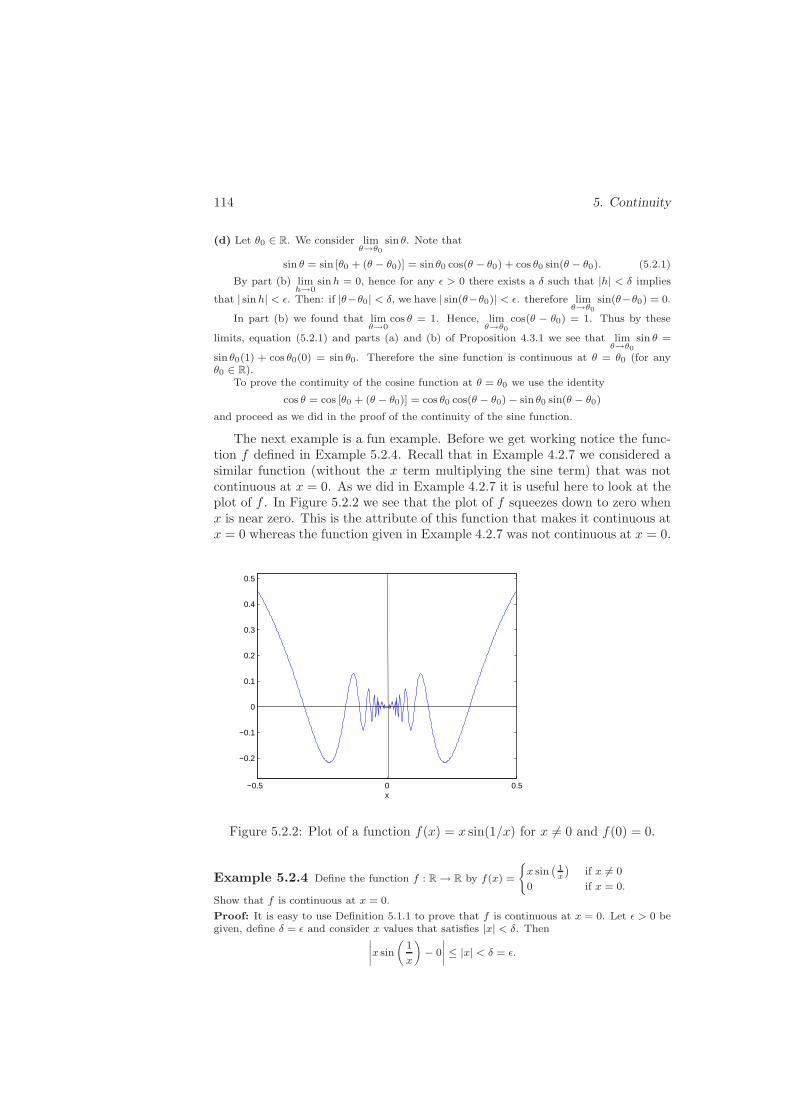
114 5. Continuity
(d) Let θ0 ∈ R. We consider limθ→θ0
sin θ. Note that
sin θ = sin [θ0 + (θ − θ0)] = sin θ0 cos(θ − θ0) + cos θ0 sin(θ − θ0). (5.2.1)
By part (b) limh→0
sinh = 0, hence for any ǫ > 0 there exists a δ such that |h| < δ implies
that | sin h| < ǫ. Then: if |θ−θ0| < δ, we have | sin(θ−θ0)| < ǫ. therefore limθ→θ0
sin(θ−θ0) = 0.
In part (b) we found that limθ→0
cos θ = 1. Hence, limθ→θ0
cos(θ − θ0) = 1. Thus by these
limits, equation (5.2.1) and parts (a) and (b) of Proposition 4.3.1 we see that limθ→θ0
sin θ =
sin θ0(1) + cos θ0(0) = sin θ0. Therefore the sine function is continuous at θ = θ0 (for anyθ0 ∈ R).
To prove the continuity of the cosine function at θ = θ0 we use the identity
cos θ = cos [θ0 + (θ − θ0)] = cos θ0 cos(θ − θ0) − sin θ0 sin(θ − θ0)
and proceed as we did in the proof of the continuity of the sine function.
The next example is a fun example. Before we get working notice the func-tion f defined in Example 5.2.4. Recall that in Example 4.2.7 we considered asimilar function (without the x term multiplying the sine term) that was notcontinuous at x = 0. As we did in Example 4.2.7 it is useful here to look at theplot of f . In Figure 5.2.2 we see that the plot of f squeezes down to zero whenx is near zero. This is the attribute of this function that makes it continuous atx = 0 whereas the function given in Example 4.2.7 was not continuous at x = 0.
−0.5 0 0.5
−0.2
−0.1
0
0.1
0.2
0.3
0.4
0.5
x
Figure 5.2.2: Plot of a function f(x) = x sin(1/x) for x 6= 0 and f(0) = 0.
Example 5.2.4 Define the function f : R → R by f(x) =
{
x sin(
1x
)
if x 6= 0
0 if x = 0.
Show that f is continuous at x = 0.
Proof: It is easy to use Definition 5.1.1 to prove that f is continuous at x = 0. Let ǫ > 0 begiven, define δ = ǫ and consider x values that satisfies |x| < δ. Then
∣
∣
∣
∣
x sin
(
1
x
)
− 0
∣
∣
∣
∣
≤ |x| < δ = ǫ.

5.3 Basic Continuity Theorems 115
Therefore f is continuous at x = 0.
It should be clear that f is also continuous for all other points in R.
We include one more example (that is also a fun example) that introducesa useful, interesting function.
Example 5.2.5 Define the function f : D = [0, 1] → R by f(x) =
{
1 if x ∈ Q
0 if x ∈ I.
Show that f is discontinuous at all points x ∈ D = [0, 1].
Solution: First consider x0 ∈ [0, 1]∩I. Let ǫ = 1/2. Consider any δ. We know by Proposition1.5.6-(a) that there exists rδ ∈ Q such that rδ ∈ (x0 − δ, x0 + δ), i.e. rδ satisfies |rδ − x0| < δand |f(rδ) − f(x0)| = |1 − 0| = 1 > ǫ = 1/2. Therefore f is not continuous at x0.
Likewise consider x0 ∈ [0, 1] ∩ Q. Let ǫ = 1/2. Consider any δ. We know by Proposition1.5.6-(b) that there exists iδ ∈ I such that iδ ∈ (x0 − δ, x0 + δ), i.e. iδ satisfies |iδ − x0| < δand |f(iδ) − f(x0)| = |0 − 1| = 1 > ǫ = 1/2. Therefore f is not continuous at x0.
HW 5.2.1 (True or Fals and why) (a) Set D = [0, 1] ∪ {3} and define f on Dby f(x) = 1 for x ∈ D ∩Q and f(x) = 0 for x ∈ D ∪ I. Then f is discontinuousat all points of D.
(b) Suppose f : [−1, 1] → R is defined as follows: for x ∈ [−1, 1]∩Q, f(x) = x2
and for x ∈ [−1, 1]∩ I, f(x) = −x2. Then the function f is continuous at x = 0.
(c) The function f defined in part (b) is discontinuous for all x ∈ [−1, 1], x 6= 0.
(d) If we consider the function f defined in Example 5.2.5, the sequence{√
22 + 1
n
}∞
n=5
can be used to show that the function f is discontinuous at x =√
2/2.
HW 5.2.2 (a) Prove that f(x) = |x− 3| is continuous at x = 3.
(b) Prove that f is continuous at x = 2.
(c) Prove that f is continuous on R.
HW 5.2.3 (a) Consider the functions f1 defined on R as f1(x) =
{
x3 x ≥ 0
3x− 1 x < 0,
f2 defined on R as f2(x) =
{
x3 x ≥ 0
3x x < 0,
and f3 defined on [−1, 1] as f3(x) =
{
x3 x ∈ [−1, 1] ∩ Q
−x3 x ∈ [−1, 1] ∩ I.At which points
are f1, f2 and f3 are continuous and show why.
HW 5.2.4 Prove that any polynomial is continuous on R.
HW 5.2.5 Prove that any rational function is continuous at all points wherethe denominator is nonzero.

116 5. Continuity
5.3 Basic Continuity Theorems
There are a lot of important continuity theorems. We will begin with the mostbasic of these theorems.
Proposition 5.3.1 Consider f, g : D → R for D ⊂ R, x0 ∈ D, c ∈ R, andsuppose that f and g are continuous at x = x0. We then have the followingresults.
(a) cf is continuous at x = x0.
(b) f ± g is continuous at x = x0.
(c) fg is continuous at x = x0.
(d) If g(x0) 6= 0, then f/g is continuous at x = x0.
Proof: The proofs of (a)-(d) follow from Proposition 5.1.3 along with Proposi-tions 3.3.2 and 3.4.1. We consider any sequence {an} such that an ∈ D for all nand an → x0. Then by the continuity hypothesis and Proposition 5.1.3 we knowthat f(an) → f(x0) and g(an) → g(x0). Then by Proposition 3.3.2 we know thatcf(an) → cf(x0), (f + g)(an) = f(an) + g(an) → f(x0) + g(x0) = (f + g)(x0)and (fg)(an) = f(an)g(an) → f(x0)g(x0) = (fg)(x0). Then by Proposition5.1.3 cf , f + g and fg are continuous at x = x0.
Likewise, for any sequence {an} such that an ∈ D for all n and an → x0,the continuity of f at x0 implies that f(an) → f(x0) and g(an) → g(x0).Since g(x0) 6= 0, Proposition 3.4.1 implies that (f/g)(an) = f(an)/g(an) →f(x0)/g(x0) = (f/g)(x0). Then by Proposition 5.1.3, f/g is continuous atx = x0.
We must realize that the above results can also be proved based on Definition5.1.1—similar to the proof of Proposition 4.3.1 given using Definition 4.1.1.Also, we want to emphasize that Proposition 5.3.1 implies that if f and g arecontinuous on D ⊂ R, then cf , f ± g, fg are continuous on D. And, f/g iscontinuous on {x ∈ D : g(x) 6= 0}—which is the natural domain of f/g.
In addition the the results given above, we also have the results analogousto parts (c) and (e) of Proposition 4.3.1. The result is a useful tool in the studyof continuity. We state the following proposition.
Proposition 5.3.2 Consider f : D → R for D ⊂ R, x0 ∈ D, and suppose thatf is continuous at x = x0.
(a) There exists a K ∈ R and δ > 0 such that |x− x0| < δ implies |f(x)| ≤ K.
(b) If f(x0) 6= 0, there exists M ∈ R and δ > 0 such that |x − x| < δ implies|f(x)| ≥M .
We don’t prove the above result—the proof is the same as those of parts (c)and (e) of Proposition 4.3.1.
The next result could be pieced together by multiple applications of partsProposition 5.3.1—but we don’t have to work that hard. We have already donethe work in Section 4.3
5.3 Basic Continuity Theorems 117
Example 5.3.1 (a) For n ∈ N the function f(x) = xn is continuous on R.(b) All polynomials are continuous on R.(c) All rational functions are continuous at all points at which the denominator is not zero.
Solution: All of the points under consideration are limit points of the domains. Then part(a) follows from Proposition 4.3.2-(c) along with Proposition 5.1.2. Parts (b) and (c) followsfrom parts (b) and (c) of Proposition 4.3.3.
The are a series of basic continuity theorems that we must consider. Weinclude the following result.
Proposition 5.3.3 Consider f, g : D → R for D ⊂ R, x0 ∈ D, c ∈ R, andsuppose that f and g are continuous at x = x0. We then have the followingresults.
(a) The function F (x) = max{f(x), g(x)} is continuous at x = x0.(b) The function G(x) = min{f(x), g(x)} is continuous at x = x0.
Proof: (a) Suppose ǫ > 0 is given. Then there exists δ1 and δ2 such that
|x− x0| < δ1 implies that |f(x) − f(x0)| < ǫ or f(x0) − ǫ < f(x) < f(x0) + ǫ(5.3.1)
and
|x− x0| < δ2 implies that |g(x) − g(x0)| < ǫ or g(x0) − ǫ < g(x) < g(x0) + ǫ.(5.3.2)
Let δ = min{δ1, δ2}. Then for x satisfying |x− x0| < δ
max{f(x0), g(x0)} − ǫ = max{f(x0) − ǫ, g(x0) − ǫ} < max{f(x), g(x)} (5.3.3)
and
max{f(x), g(x)} < max{f(x0) + ǫ, g(x0) + ǫ} = max{f(x0), g(x0)} + ǫ (5.3.4)
or F (x0) − ǫ < F (x) < F (x0) + ǫ. Thus we have |F (x) − F (x0)| < ǫ so F iscontinuous at x = x0. Look at the computation given in (5.3.3) and (5.3.4)carefully. It’s easy but looks difficult. You start with max{f(x), g(x)} andreplace each of them by the inequalities given by statements (5.3.1) and (5.3.2).
(b) Of course the proof of part (b) will be the same. We again consider state-ments (5.3.1) and (5.3.2). This time taking the minimums, we get G(x0) − ǫ <G(x) < G(x0) + ǫ or |G(x) −G(x0)| < ǫ. Thus G is continuous at x = x0.
Next we want to give a result that will expand the number of functions thatwe know are continuous. Before we give the result we include the definition ofthe composite function.
Definition 5.3.4 For D ⊂ R consider f : D → R and g : U → R wheref(D) ⊂ U . Then the composition of f and g, g ◦ f : D → R is defined asg ◦ f(x) = g(f(x)) for all x ∈ D.
118 5. Continuity
We use the composition to define some more interesting functions: (i) f(x) =x2 + 1 and g(y) =
√y implies that g ◦ f(x) = sqrtx2 + 1. (ii) f(θ) = θ − π/2
and g(y) = sin y implies that g ◦ f(θ) = sin(θ − π/2). etc. We then have thefollowing basic result concerning continuity of the composite function.
Proposition 5.3.5 Suppose that f : D → R, g :→ R, f(D) ⊂ U , f is continu-ous at x0 and g is continuous at f(x0). Then g ◦ f is continuous at x = x0.
Proof: We suppose that ǫ > 0 is given. g continuous at f(x0) implies thatthere exists a δ1 such that |y− f(x0)| < δ1 implies that |g(y)− g(f(x0))| < ǫ. fcontinuous at x0 (applying the definition of the continuity of f at x0 using δ1 inplace of the traditional ”ǫ”) implies that there exists a δ such that |x− x0| < δimplies that |f(x) − f(x0)| < δ1.
Then for x−x0| < δ we have |f(x)−f(x0)| < δ1 which implies that |g(f(x))−g(f(x0))| < ǫ or g ◦ f is continuous at x = x0.
We next define the maximum and minimums that you worked a lot with inyour basic course.
Definition 5.3.6 Consider the function f : D → R where D ⊂ R and x0 ∈ D.(a) The point (x0, f(x0)) is said to be a maximum (or local maximum) of f ifthere exists a neighborhood of x0, N , such that f(x) ≤ f(x0) for all x ∈ N ∩D.(b) The point (x0, f(x0)) is said to be an absolute maximum of f on D if f(x) ≤f(x0) for all x ∈ D.(c) The point (x0, f(x0)) is said to be a minimum (or local minimum) of f ifthere exists a neighborhood of x0, N , such that f(x) ≥ f(x0) for all x ∈ N ∩D.(d) The point (x0, f(x0)) is said to be an absolute minimum of f on D if f(x) ≥f(x0) for all x ∈ D.
It is easy to see that the function f(x) = −x2 defined on [−1, 1] has a maxi-mum at (0, 0)—it is an absolute maximum. This function has minimums at bothpoints (−1,−1) and (1,−1)—which are both absolute maximums. Note thatthis means that the absolute maximum or minimum need not be unique. Notethat the same function defined on the set (−1, 1) does not have any minimi—and then surely does not have an absolute minimum. We also note that if wedefine a function f : D → R, D = (−2,−1)∪{0}∪ (1, 2), by f(x) = x2, then bythe definition x = 0 is both a maximum and a minimum—not very satisfyingbut acceptable.
We next prove a useful lemma and an very important theorem concerningcontinuous functions.
Lemma 5.3.7 Suppose that f : [a, b] → R and f is continuous on [a, b]. Thenthere exists an M ∈ R such that f(x) ≤M for all x ∈ [a, b].
Proof: Suppose false. Suppose there is not such M such that f(x) ≤M .For M = 1 there exists an x1 ∈ [a, b] such that f(x1) > 1 (otherwise M = 1would work).For M = 2 there exists an x2 ∈ [a, b] such that f(x2) > 2.
5.3 Basic Continuity Theorems 119
And, in general, for each n ∈ N there exists an xn ∈ [a, b] such that f(xn) > n.{xn} is a sequence in [a, b]. Since [a, b] is compact, by Corollary 3.4.8 we knowthat the sequence {xn} has a subsequence, {xnj} and there is an x0 ∈ [a, b],such that xnj → x0 as j → ∞. Then by the continuity of f on [a, b] andProposition 5.1.3 we know that f(xnj ) → f(x0). Since the sequence {f(xnj}∞j=1
is convergent, we know by Proposition 3.3.2–(c) that the sequence is bounded.This contradicts the fact that f(xnj ) > nj > j for all j. Therefore the setf([a, b]) is bounded above.
Theorem 5.3.8 Suppose that f : [a, b] → R and f is continuous on [a, b]. Thenf has an absolute maximum and an absolute minimum on [a, b].
Proof: Let S = f([a, b]). By Lemma 5.3.7 S is bounded above. Thus by thecompleteness axiom, Definition 1.4.3, M∗ = lub(S) exists. Note that to find anabsolute maximum of f on [a, b], we must find an x0 such that f(x0) = M∗.
Recall that by Proposition 1.5.3–(a) for every ǫ > 0 there exists an s ∈ Ssuch thatM∗−s < ǫ. In our case Proposition 1.5.3–(a) gives that for every ǫ > 0there exists an x ∈ [a, b] (and an associated f(x)) such that M∗ − f(x) < ǫ—allpoints in S look like f(x)—and are associated with an x ∈ [a, b].
Let ǫ = 1. We get x1 ∈ [a, b] such that M∗ − f(x1) < 1.
Let ǫ = 1/2. We get x2 ∈ [a, b] such that M∗ − f(x2) < 1/2.
In general, let ǫ = 1/n for n ∈ N. We get xn ∈ [a, b] such that M∗−f(xn) < 1/n.
Hence we have M∗ − 1/n < f(xn) ≤M∗ for all n ∈ N (because M∗ is an upperbound) so f(xn) →M∗.
All of xn’s are in [a, b]. Since [a, b] is compact, by Corollary 3.4.8 we knowthat there exists a subsequence of {xn}, {xnj}, such that xnj → x0 for somex0 ∈ [a, b]. Thus f(xnj ) → f(x0).
By Proposition 3.4.6 we know that f(xnj ) → M∗. By Proposition 3.3.1 weknow that the limit must be unique. Thus M∗ = f(x0) and (x0, f(x0)) is anabsolute maximum.
To show that f has an absolute minimum on [a, b] we consider the functiong = −f . If f is continuous on [a, b], the function g will be continuous on [a, b].The absolute maximum of g on [a, b] will be the absolute minimum of f on [a, b].
From the above theorem we obtain the following useful corollary.
Corollary 5.3.9 If f : [a, b] → R is continuous on [a, b], then f is bounded on[a, b].
HW 5.3.1 (True or False and why) (a) Suppose f, g : D → R, D ⊂ R, x0 ∈ R.If f and g are continuous at x = x0, then either f or g is continuous at x = x0.(b) Suppose f : [0, 1] → R such that f2 is continuous on [0, 1]. Then f iscontinuous on [0, 1].

120 5. Continuity
(c) Suppose f, g : D → R, D ⊂ R. Then max{f(x), g(x) : x ∈ D} = max{f(x) :x ∈ D}max{g(x) : x ∈ D}.
(d) Consider f(x) =√x defined on [0,∞) and g(x) = x− 1 defined on R. Then
f ◦ g is continuous on [1,∞).(e) Consider f : [0, 1] → R. Then f has a maximum on [0, 1].
HW 5.3.2 Suppose that f : [0, 1] → R is continuous at the point x = x0 andf(x0) > 0. Prove that there exists an n ∈ N such that f(x) > 0 for all x in theneighborhood N1/n(x0).
HW 5.3.3 (a) Suppose f : D → R, D ⊂ R, x0 ∈ D, is continuous at x = x0.Prove that |f | (defined by |f |(x) = |f(x)|) is continuous at x = x0.(b) Prove that for x ∈ D min{f(x), g(x)} = 1
2 [f(x) + g(x)] − 12 |f(x) − g(x)|.
(c) If f and g are continuous at x = x0, prove that G(x) = min{f(x), g(x)}is continuous at x = x0 (give a proof different from that given in Proposition5.3.3).
5.4 More Continuity Theorems
We next prove a very important basic theorem concerning continuous functions—the result yields an approximate characterisation of continuity.
Theorem 5.4.1 (Intermediate Value Theorem: IVT) Suppose that f : [a, b] →R and f is continuous on [a, b]. Let c ∈ R be between f(a) and f(b). Then thereexists x0 ∈ (a, b) such that f(x0) = c.
Proof: We have two cases, f(a) < c < f(b) and f(b) < c < f(a). We willconsider the first case—the second case will follow in the same way.
This will be a constructive proof. Let a1 = a and b1 = b.
Let m1 = (a1 + b1)/2. If f(m1) ≤ c, define a2 = m1 and b2 = b1. If f(m1) > c,define a2 = a1 and b2 = m1. Note that this construction divides the intervalin half, and chooses the half so that f(a2) ≤ c < f(b2)—specifically we havea = a1 ≤ a2 < b2 ≤ b1 = b and f(a2) ≤ c < f(b2).
Let m2 = (a2 + b2)/2. If f(m2) ≤ c, define a3 = m2 and b3 = b2. If f(m2) > c,define a3 = a2 and b3 = m2. We have a = a1 ≤ a2 ≤ a3 < b3 ≤ b2 ≤ b1 = b andf(a3) ≤ c < f(b3).
We continue in this fashion and inductively obtain an and bn, n = 1, 2, · · ·such that
a = a1 ≤ a2 ≤ a3 ≤ · · · ≤ an < bn ≤ bn−1 ≤ · · · ≤ b1 = b
and f(an) ≤ c < f(bn).We have a sequence of closed intervals [an, bn] such that f(an) ≤ c < f(bn)
and bn − an = 12 [bn−1 − an−1] = · · · = 1
2n−1 [b1 − a1] = 12n−1 [b− a].
Clearly {an} is a monotonically increasing sequence that is bounded aboveby b. Therefore by the Monotone Convergence Theorem, Theorem 3.5.2, there
5.4 More Continuity Theorems 121
exists α ≤ b such that an → α. Likewise the sequence {bn} is a monotonicallydecreasing sequence bounded below by a. Thus by the Monotone ConvergenceTheorem there exists a β ≥ a such that bn → β.
We see that limn→∞[bn − an] = limn→∞1
2n−1 [b − a] = 0 and limn→∞[bn −an] = β − α. Thus α = β. Call it x0
We have f(an) ≤ c < f(bn) and limn→∞ f(an) = limn→∞ f(bn) = f(x0).By the Sandwhich Theorem, Proposition 3.4.2, (where the center sequence willbe the constant sequence {c, c, · · · }) we have f(x0) = c.
We might note that one of the nice applications of the IVT is to prove theexistence of a solution of an equation of the form f(x) = 0. The approach is tofind a and a b in the domain of the function such that f(a) < 0, f(b) > 0 and fis continuous on [a, b]. The IVT then implies that there exists an x0 ∈ [a, ] suchthat f(x0) = 0. For example consider the function f(x) = x5 + x+ 1. We notethat f(−1) = −1, f(1) = 3 and f is surely continuous on the interval [−1, 1].Therefore by the Intermediate Value Theorem there exists an x0 ∈ [−1, 1] suchthat f(x0) = 0. Can you find such an x0. Can you approximate it? (Use yourcalculator.)
A slight variation of the above application of the IVT and essentially theprocess that we used for the proof of the IVT gives us an excellent methodfor finding an approximation to the solution to an equation f(x) = 0: calledthe Bisection Method. Suppose we know that f(a) < 0, f(b) > 0 and f iscontinuous on [a, b]. We then use a construction that we have used in the proofof the IVT. We set a1 = a and b1 = b.
We set c1 = (a1 + b1)/2 and evaluate f(c1). If f(c1) < 0, we set a2 = c1 andb2 = b1. If f(c1) > 0, we set a2 = a1 and b2 = c1. (If f(c1) ≈ 0, quit.)
We set c2 = (a2 + b2)/2 and evaluate f(c2). If f(c2) < 0, we set a3 = c2 andb3 = b2. If f(c2) > 0, we set a3 = a2 and b3 = c2. (If f(c2) ≈ 0, quit.)
We continue in this fashion until for some cn, f(cn) is sufficiently small.We use that value of cn as an approximation of the solution of f(x) = 0. Wenote that the proof of the IVT proves that the sequence {an} converges to thesolution of f(x) = 0. (It’s easy to see that the sequence {cn} will also convergeto the solution of f(x) = 0.) We really don’t know how fast this convergenceis taking place (the Bisection method is not the fastest method) but we canget an excellent approximation to solutions of equations using this method. Forexample if we again consider f(x) = x5 + x + 1, set a = −1 and b = 1, andperform the iteration, we get c1 = 0.0, c2 = −0.5, c3 = −0.75, c4 = −0.875,c5 = −0.8125, c6 = −0.7813, c7 = −0.7656, c8 = −0.7578. We see thatf(−0.7578) = −0.0077 and we stopped because we chose ”sufficiently small”to be 0.01. And of course, if you wanted to find the solutions to x5 + x+ 1 = 7instead, you could consider f(x) = (x5 + x+ 1) − 7.
We next include a corollary to Theorem 5.4.1 that will be useful to us inthe next section. Before we proceed we want to emphasize that by interval, wemean any of the different types of intervals we have introduced—closed, open,part open and part closed, unbounded, etc. We state the following result.

122 5. Continuity
Corollary 5.4.2 Suppose f : I → R where I ⊂ R is an interval and f iscontinuous on I. Then f(I) is an interval.
Proof: If f(I) is not an interval, there must be an f(a), f(b) ∈ f(I) and ac ∈ R such that c is between f(a) and f(b) but c 6∈ f(I). This would contradictTheorem 5.4.1 applied to f on [a, b] (where for convenience we assume thata < b).
Often we are interested in when and where the functions are increasing anddecreasing—if you recall, you probably used these ideas in your basic class whenyou used calculus to plot the graphs of some functions. We will use these ideasin a very powerful way to help us study the inverse of functions. Before weproceed we make the following definitions.
Definition 5.4.3 Consider the function f : D → R where D ⊂ R.
(a) f is said to be increasing on D if for x, y ∈ D such that x < y, thenf(x) ≤ f(y).
(b) f is said to be decreasing on D if for x, y ∈ D such that x < y, thenf(x) ≥ f(y).
(c) f is said to be strictly increasing on D if for x, y ∈ D such that x < y, thenf(x) < f(y).
(d) f is said to be strictly decreasing on D if for x, y ∈ D such that x < y, thenf(x) > f(y).
If the function f is either increasing or decreasing, we say that f is mono-tone. If f is either strictly increasing or decreasing, then we say that f is strictlymonotone.
We note that f2(x) = x2 is not monotone on R. We also note that f2is strictly increasing on [0,∞) and strictly decreasing on (−∞, 0]. We alsonote that f3(x) = x3 is strictly increasing on R—these all can be seen bygraphing the functions—these all can be proved by using the methods similarto those used in HW1.3.3-(a). A more complicated function is given by f7(x) ={
x− 4 if x < 0
2x+ 3 if x ≥ 0—graph it and it should be clear that f7 is increasing on R.
If we define f8(x) =
−x+ 4 if x < 0
2 if 0 ≤ x ≤ 1
−4x if x > 1
and graph it, it is easy to see that
f8 is decreasing but not strictly decreasing.
We next prove a result we think is surprising in that we get continuity witha rather strange hypothesis. Read this proof carefully—it is a very technicalproof.
Proposition 5.4.4 Consider f : D → R where D ⊂ R. Assume that f ismonotone on D. If f(D) is an interval, then f is continuous on D.

5.4 More Continuity Theorems 123
Proof: Consider the case when f is increasing. The case of f decreasing willbe the same. Let x0 ∈ D and suppose that ǫ > 0 is given. We must find a δ sothat |x− x0| < δ implies that |f(x) − f(x0)| < ǫ, i.e.
f(x0) − ǫ < f(x) < f(x0) + ǫ. (5.4.1)
Since we know that f is increasing to the right of x0, we limit δ so that forx ∈ (x0, x0 + δ) f cannot grow too much (not more than to f(x0)+ ǫ). We thendo the same thing to the left of x0.
Consider the right most part of inequality (5.4.1): f(x) < f(x0) + ǫ.
If f(x) ≤ f(x0) for all x ∈ D, the desired inequality is satisfied and we canchoose δ1 = 1.
Otherwise, let x∗ ∈ D be such that f(x∗) > f(x0). Then x0 < x∗ (becausef is increasing) and the interval [f(x0), f(x∗)] is contained in f(D) (f(D) isassumed to be an interval). Let y∗∗ = min{f(x0) + ǫ/2, f(x∗)}. Then theinterval [f(x0), y
∗∗] is contained in f(D). Thus there exists an x∗∗ ∈ D suchthat f(x∗∗) = y∗∗. Then x0 < x < x∗∗ implies that f(x0) ≤ f(x) ≤ f(x∗∗) =y∗∗ < f(x0) + ǫ. Let δ2 = x∗∗ − x0.
Now consider the left most part of inequality (5.4.1): f(x0) − ǫ < f(x).
If f(x) ≥ f(x0), we are done. Let δ3 = 1.
Otherwise, let x∗ be such that f(x∗) < f(x0). Then x∗ < x0 and the interval[f(x∗), f(x0)] ⊂ f(D). Let y∗∗ = max{f(x0) − ǫ/2, f(x∗)}. Then [y∗∗, f(x0)] ⊂f(D) and there exists x∗∗ ∈ D f(x∗∗) = y∗∗. Then x∗∗ < x < x0 implies thatf(x0) − ǫ < y∗∗ = f(x∗∗) ≤ f(x) ≤ f(x0). Let δ4 = x0 − x∗∗.
Thus we see that if we define δ = min{δ1, δ2, δ3, δ4} (Define δ) and requirethat |x− x0| < δ, then |f(x) − f(x0)| < ǫ.
Notice that the functions f7 and f8 consider earlier are both monotone butare not continuous—neither f7(R) nor f8(R) are intervals. Check it out.
We next state a result is a bit strange because we already have this result—itis a combination of Corollary 5.4.2 and Proposition 5.4.4. We do so because wewant to emphasize this result in this form.
Corollary 5.4.5 Consider f : I → R where I ⊂ R is an interval. Assumethat f is monotone on I. Then f is continuous on I if and only if f(I) is aninterval.
There are times when we are given a function, it is very important to use toknow that the function has an inverse and to be able to determine propertiesof that inverse. You have been using inverse functions for a long time(it is avery basic result to be give some y = f(x) and want to solve for x—sometimesyou might have been aware that you were using an inverse, and other times youmight not have been aware. We begin with the following definition.
Definition 5.4.6 Consider f : D → R where D ⊂ R. The function f is saidto be one-to-one (often written 1-1) if f(x) = f(y) implies that x = y.

124 5. Continuity
In your basic calculus course when you studied one-to-one functions you usedwhat is called the horizontal line test—that is, draw an arbitrary horizontal lineon the graph of the function, the function is one-to-one if the line intersectsthat graph at only one point. It should be clear that this description of thehorizontal line test is equivalent to Definition 5.4.6—though less rigorous.
To prove that function f1(x) =√x defined on [0,∞) we note that f1(x) =
f1(y) is the same as√x =
√y. If we then square both sides, we find that
x = y—which is what we must prove. Graph f1 to see how the horizontal linetest works. The function f2(x) = x2 is surely not one-to-one on R. Again, plotthe function and draw the horizontal line. If we consider f2 on [0,∞) instead,then f2 is one-to-one.
A statement that is equivalent to Definition 5.4.6 is as follows: The functionf is said to be one-to-one for each element y ∈ f(D) there exists one and onlyone element in D, x, such that f(x) = y. The definition of one-to-one allows usto make the following definition.
Definition 5.4.7 Consider f : D → R where D ⊂ R. Assume that the functionf is one-to-one. We define the function f−1 : f(D) → D by f−1(y) = x iff(x) = y. The function f−1 is called the inverse of f . When f−1 exists, f issaid to be invertible.
Note that the definition that f is one-to-one is exactly what is needed to makef−1 a function, i.e. for each y ∈ f(D)there exists one and only one x ∈ D suchthat f−1(y) = x. We also note that by rewriting the statement in Definition5.4.7 we see that f and f−1 satisfy f−1(f(x)) = x for x ∈ D and f(f−1(y)) = yfor y ∈ f(d).
If we consider f2(x) = x2 on [0,∞), let y = x2 and solve for x, we getx = ±√
y. Since x must be greater than or equal to zero, f−12 (y) =
√y. Note
that since f2([0,∞)) = [0,∞), the domain of f−12 is also [0,∞). If we next
consider f3(x) = x3 on R, we note that f3(R) = R and f−13 (y) = 3
√y for all
y ∈ R.We obtain the following important but very easy result.
Proposition 5.4.8 Consider f : D → R where D ⊂ R. Assume that f isstrictly monotone on D. Then f is one-to-one on D.
Proof: Suppose that f is strictly increasing—the proof for f strictly decreasingwill the same—and suppose that f is not one-to-one. Then there exists x 6= ysuch that f(x) = f(y). If x 6= y, then either x < y or y < x—either case is acontradiction to the fact that f is strictly increasing.
It’s clear that the converse of Proposition 5.4.8 is not true when we considera function like f(x) = 1/x defined on R − {0}. However we are able to obtainthe following result.
Proposition 5.4.9 Consider the function f : I → R where I ⊂ R is an in-terval. Assume that f is one-to-one and continuous on I. Then f is strictlymonotone on I.

5.4 More Continuity Theorems 125
Proof: We begin by choosing arbitrary a, b ∈ I. For convenience assume thata < b. Since f is one-to-one, we know that f(a) 6= f(b)—so that either f(a) <f(b) or f(a) > f(b). Consider the case of f(a) < f(b). If f is to be strictlymonotone, in this situation it must be the case that f is strictly increasing on[a, b]. Assume false, i.e. assume that f is not strictly increasing on [a, b], i.e.assume there exists some x1, x2 ∈ [a, b] such that x1 < x2 and f(x1) ≥ f(x2)—since f is one-to-one, we know we would really have f(x1) > f(x2).
We have two cases. For each case it might help to draw a picture ofthe situation—give it a try. Case 1: f(a) < f(x1). We then choose c =max{(f(x1)+ f(x2))/2, (f(a)+ f(x1))/2}. Since f is continuous on I, f is con-tinuous on [a, x1]. Also c is between f(a) and f(x1). Therefore by the IVT,Theorem 5.4.1, we know that there exists y1 ∈ [a, x1] such that f(y1) = c.
Also f is continuous on [x1, x2] and c is between f(x1) and f(x2). Thusagain by the IVT we know that there exists y2 ∈ [x1, x2] such that f(y2) = c.This is a contradiction to the fact that f is one-to-one.
Case 2: f(a) > f(x1). In this case then f(b) > f(a) > f(x1) > f(x2). Similarto the last case, we set c = min{(f(x1) + f(x2))/2, (f(x2) + f(b)/2}, apply theIVT with respect to c on [x1, x2] and [x2, b], and arrive at a contradiction to thefact that f is one-to-one on I.
Therefore f is strictly increasing on I.
The case when f(a) > f(b) is essentially the same.
Proposition 5.4.10 Suppose that f : D → R and D ⊂ R. (a) If f is strictlyincreasing on D, then f−1 : f(D) → D is strictly increasing on f(D).(b) If f is strictly decreasing, then f−1 : f(D) → D is strictly decreasing onf(D).
Proof: (a) We assume that f−1 is not strictly increasing, i.e. supposethat u < v and f−1(u) 6< f−1(v). Then f−1(u) ≥ f−1(v). Suppose x and yare such that f(x) = u and f(y) = v. Then u < v implies f(x) < f(y) andf−1(u) ≥ f−1(v) implies that x ≥ y.
This contradicts the fact that f is increasing because when f is increasingx > y implies f(x) > f(y) and x = y implies f(x) = f(y). i.e. if we have x ≥ y,we have f(x) ≥ f(y).
(b) The proof when f is strictly decreasing is very similar to that given in part(a).
The next two results are the ultimate results relating the continuity proper-ties of f−1 to those of f .
Proposition 5.4.11 Suppose that I ⊂ R is an interval and f : I → R is strictlymonotone on I. Then f−1 : f(I) → I is continuous.
Proof: Suppose that f is strictly increasing—the proof of the case for f strictlydecreasing is the same. We know then by Proposition 5.4.10–(a) that f−1 :f(I) → I is strictly increasing. Then since f−1(f(I)) = I is an interval (and
126 5. Continuity
f(I) is the domain of f−1), by Proposition 5.4.5 we see that f−1 is continuouson f(I).
Proposition 5.4.12 Suppose that f : I → R where I ⊂ R. Assume that f isone-to-one and continuous on I. Then f−1 : f(I) → I is continuous.
Proof: This is an easy combination of Propositions 5.4.9 and 5.4.11. FromProposition 5.4.9 we see that f is strictly monotone on I. Then by Proposition5.4.11 we have that f−1 is continuous on f(I).
The results of the two propositions—f−1 is continuous—is the same. Thedifference between the two propositions is in the hypotheses. The fact thatwe assume f continuous (and one-to-one) in Proposition 5.4.12 is a strongerhypothesis than assuming strict monotonicity as we do in Proposition 5.4.11.However, there are times that it is preferable to be able to assume one-to-one than monotonicity—and it’s not a terrible assumption to assume that f iscontinuous. The real point is that we have both results. Whatever we want touse in the end, we will have.
HW 5.4.1 (True or False and why) (a) There is at least one solution to theequation x4 − 3x3 + 2x2 − x− 1 = 0.
(b) Consider the function f : R → R defined by f(x) = sinx. We know thatf(R) = [−1, 1] is an interval. Then f is invertible on [−1, 1].
(c) Suppose f : D → R, D ⊂ R, is one-to-one and continuous on D. Then f isstrictly monotone.
(d) Suppose f : D → R, D ⊂ R, is monotone. Then f is invertible.
(e) Suppose f : D → R, D ⊂ R, is continuous on D. Then f(D) is an interval.
HW 5.4.2 Prove that the equation x6 + x4 − 3x3 − x+ 1 = 0 has at least onesolution. Find an approximation of a solution to the equation.
HW 5.4.3 Suppose that the function f : [0, 1] → R is continuous and satisfiesf([0, 1]) ⊂ Q. Prove that f is the constant function.
HW 5.4.4 Can we put in the M161 problem?
HW 5.4.5 Define the function f(x) =
{
3x− 2 if x < 0
2x+ 1 if x ≥ 0.
(a) Show that the function f is strictly increasing.
(b) Determine f(R).
(c) Show that f−1 exists.
(d) Prove that f−1 is continuous at x = −2.
(e) Determine where f−1 is continuous.

5.5 Uniform Continuity 127
5.5 Uniform Continuity
The set of continuous functions on some domain D is an important set of func-tions. There is another level of smoothness that we attach to functions thatyields another important class of functions: uniformly continuous functions. Aswe shall see the idea of uniform continuity is truly related to the set D whereascontinuity was defined pointwise and then was consider continuous on the set Dif it was continuous at each individual point of D. We begin with the definition.
Definition 5.5.1 Consider the function f : D → R where D ⊂ R. f is saidto be uniformly continuous on D if for every ǫ > 0 there exists a δ such thatx, y ∈ D and |x− y| < δ implies that |f(x) − f(x0)| < ǫ.
This definition should be observed carefully and contrasted with Definition 5.1.1.If we consider the function f(x) = x2 defined on D = (0, 1), we hope that it isclear that f is continuous on (0, 1). However, when we proceed to show that itis continuous at each point in (0, 1), we might begin by considering x0 = 0.1.Then given ǫ > 0 we write |x2 − (0.1)2| = |x− 0.1||x+ 0.1| and realize that thisis one of the applications of the definition of continuity where we must restrictthe range of x and bound the term |x+0.1|. Suppose we let δ1 = 0.1 (no specifictie to the fact that x0 = 0.1 except for the fact that both were chosen because0.1 is a nice small number) and restrict x so that |x − 0.1| < δ1 = 0.1. Then|x+ 0.1| < 3/10 so we set δ0.1 = min{0.1, 10ǫ/3}, suppose that |x − 0.1| < δ0.1and continue with our previous calculation to get
|x2 − (0.1)2| = |x− 0.1||x+ 0.1| <∗ (3/10)|x− 0.1| <∗∗ (3/10)10ǫ/3 = ǫ
where the ”<∗” inequality is true because δ0.1 ≤ 0.1 and the ”<∗∗” inequalityis true because δ0.1 ≤ 10ǫ/3. Therefore f(x) = x2 is continuous at x = 0.1.
If we continued by next choosing x0 = 0.9, we can do some work to notethat we can choose δ0.9 = min{0.1, 10ǫ/19}, suppose that |x − 0.9| < δ0.9 andnote that
|x2 − (0.9)2| = |x− 0.9||x+ 0.9| < (19/10)|x− 0.9| < (19/10)10ǫ/19 = ǫ.
Therefore f is continuous at x = 0.9. (Do the necessary calculation.)To continue with showing that f is continuous on D = (0, 1) we have many
more points to consider. But let us consider the two points we have alreadyconsidered. We first admit that we could have bounded our x values differently(chosen δ1 larger than 0.1) and gotten different δ’s—but that wouldn’t makeour point. The end result is that we prove continuity at these two points usingradically different δ’s. For example, if ǫ = 0.001, then δ0.1 = (0.001)10/3 andδ0.9 = (0.001)10/19. Not only do we get different δ’s, in this case we get radicallydifferent δ’s.
When we want to prove that f(x) = x2 is uniformly continuous onD = (0, 1),for a given ǫ > 0 we must find a δ so that for any x, y ∈ (0, 1) and |x − y| < δimplies that |x2 − y2| < ǫ. That means it must work when we choose y = 0.1and it must work when we choose y = 0.9. It seems as if (we don’t really know
128 5. Continuity
for sure) δ0.1 will not work everywhere because it is a lot bigger than the δ0.9.Since the δ0.9 < δ0.1, δ0.9 would work at both y = 0.1 and y = 0.9. Is there anyreason to believe that it would work everywhere? If a function f is continuouson a set D and we are given an ǫ > 0, it is perfectly permissable for the δ to bedifferent at every point in D.
Thus the question is can we choose a δ that will work everywhere (if wecan’t, then f is not uniformly continuous on (0, 1)) and how do we do it. Ifwe return to Figure 4.1.1 and consider what determines the size of δ (in thecase of Figure 4.1.1, the δ1 and the δ2) it should be clear that the steepnessof the graph at and near the point is what determines the quantity needed forδ—the steeper the curve the smaller the δ. Hence, we want to choose the pointof D = (0, 1) that requires the smallest δ, i.e. the point at which the graph isthe steepest, construct a continuity at that point to determine the δ and showthat this δ will work for x, y ∈ D.
Hopefully we know what the graph of f(x) = x2 looks like on (0, 1). It shouldbe clear that there is not a point in (0, 1) at which the graph is the steepest, butit is also clear that the closer we get to x = 1, the steeper the curve gets. Weconsider the point x0 = 1. But this is ridiculous because x0 = 1 6∈ D = (0, 1).Who cares. If we can determine a δ that works, we will be done. We know thatf(x) = x2 could have just as well been defined on all of [0, 1] so a continuityproof at x0 = 1 will make sense. We again consider |x2 − (1)2| = |x− 1||x+ 1|.If we restrict x so that |x − 1| < δ1 = 0.1 or 0.9 < x < 1.1, then for x ∈ [0, 1],|x+1| ≤ 2.1. We then set δ = min{0.1, ǫ/2.1}, suppose that x satisfies x ∈ [0, 1]and |x− 1| < δ and continue with our previous calculation to get
|x2 − 1| = |x− 1||x+ 1| ≤ 2.1|x− 1| < 2.1ǫ/2.1 = ǫ.
Thus, if we considered f(x) = x2 defined on [0, 1], we would know that f iscontinuous at x0 = 1.
We now have a δ = min{0.1, ǫ/2.1} that our earlier argument indicatesmight work to show that f is uniformly continuous on (0, 1). We suppose thatx, y ∈ D = (0, 1) satisfies |x − y| < δ and consider |f(x) − f(y)| = |x2 − y2| =|x− y||x+ y|. Clearly for x, y ∈ (0, 1), |x+ y| < 2. Thus we have
|f(x) − f(y) = |x2 − y2| = |x− y||x+ y| < 2|x− y| < 2δ ≤ 2ǫ/2.1 < ǫ.
Therefore f is uniformly continuous on D = (0, 1).
In summary we see that when we prove that a function is continuous on a set,the derived δ may be different at each point of the set. To prove uniform con-vergence we must find a δ that works uniformly through out the entire domain.We saw that if a function is going to be uniformly continuous, one way to findthe correct δ is to consider continuity at the steepest point of the graph of thefunction. More so, in the example considered above we first literally proved (atleast determined the correct δ) uniform convergence of f(x) = x2 on the largerdomain [0, 1]—and then used this information to prove uniform convergence on(0, 1). In effect, we used the following proposition which is trivial to prove.

5.5 Uniform Continuity 129
Proposition 5.5.2 Suppose the function f : D → R, D ⊂ R is uniformlycontinuous on D. If D1 ⊂ D, then f is uniformly continuus on D1.
One very important but easy result is the following.
Proposition 5.5.3 Suppose the function f ;D → R, D ⊂ R is uniformly con-tinuous on D. If x0 is any point in D, then f is continuous at x = x0.
It should be pretty clear how we find a function that is not uniformlycontinuous—a function that doesn’t have a steepest point, the graph keeps get-ting steeper and steeper. Consider the function f : D = (0, 1) → R defined byf(x) = 1/x. It is not difficult to show that f is continuous on D. It’s more diffi-cult to show that f is not uniformly continuous. We suppose that f is uniformlycontinuous on D = (0, 1). Then for a given ǫ > 0 there must exist a δ such that
|x − y| < δ implies
∣
∣
∣
∣
1
x− 1
y
∣
∣
∣
∣
. Consider any δ > 0. Clearly the graph gets steep
near x = 0 so that’s where we have to work. Consider the points xn = 1/n and
yn = 1/2n. Then |xn−yn| = 1/2n and |f(xn)−f(yn)| =∣
∣
∣
1xn
− 1yn
∣
∣
∣= n. Clearly
we can find an n such that 1/2n < δ (and this will hold for all larger n) and such
that n > ǫ. For this value of n we have |xn − yn| < δ and
∣
∣
∣
∣
1
xn− 1
yn
∣
∣
∣
∣
= n > ǫ.
Thus f is not uniformly continuous on (0, 1).There is a result that makes this last proof a bit easier. Since it is an ”if and
only if” result, the following proposition provides for an alternative definitionof uniform continuity.
Proposition 5.5.4 Suppose the function f : D → R, D ⊂ R. The function fis uniformly continuous if and only if for all sequences {un}, {vn} in D suchthat lim
n→∞[un − vn] = 0, then lim
n→∞[f(un) − f(vn)] = 0.
Proof: (⇒) Let ǫ > 0 be given. Since f is uniformly continuous on D, thereexists δ such that x, y ∈ D and |x− y| < δ implies that |f(x) − f(y)| < ǫ.
Suppose that {un} and {vn} are two sequences inD such that limn→∞
[un − vn] =
0. Apply the definition of the limit of a sequence to this statement. Let ǫ1 = δ(where we have used ǫ1 because we have already used ǫ). Then there exists anN ∈ R such that n > N implies that |un − vn| < δ. Then for n > N we have|un − vn| < δ so we can apply the definition of uniform continuity given aboveto get |f(un) − f(vn)| < ǫ and of course this holds for all n > N . Thereforelimn→∞
[f(un) − f(vn)] = 0.
(⇐) Suppose f is not uniformly continuous on D, i.e. suppose that for someǫ0 > 0 for any δ there exist x, y ∈ D such that |x−y| < δ and |f(x)−f(y)| ≥ ǫ0.We inductively define two sequences in the following manner.Set δ = 1. Then there exists x1, y1 ∈ D such that |x1 − y1| < δ and |f(x1) −f(y1)| ≥ ǫ0.Set δ = 1/2. Then there exists x2, y2 ∈ D such that |x2 − y2| < δ and |f(x2) −f(y2)| ≥ ǫ0.

130 5. Continuity
In general set δ = 1/n. Then there exists xn, yn ∈ D such that |xn − yn| < δand |f(xn) − f(yn)| ≥ ǫ for all n ∈ N.
We have two sequences {xn}, {yn} such that xn − yn → 0 as n → ∞ andf(xn) − f(yn) 6→ 0. This is a contradiction—to the hypothesis.
We feel that when the above statement is used as the definition it is a ratherodd definition. However, Proposition 5.5.4 gives us an excellent approach toshow that a function is not uniformly continuous. For the example consideredearlier, f(x) = 1/x defined on D = (0, 1), we define un = 1/n and vn = 1/2n.Then
limn→∞
[un − vn] = limn→∞
[
1
n− 1
2n
]
= limn→∞
1
2n= 0
and
limn→∞
[f(un) − f(vn)] = limn→∞
(n− 2n) = − limn→∞
n = −∞ (not zero).
Thus by Proposition 5.5.4 f is not uniformly continuous on D = (0, 1). Notethat this is essentially what we did earlier—but now we have a proposition thatwe can easily apply.
We next include a result that is a logical and necessary result—we had ananalogous result for limits and continuity.
Proposition 5.5.5 Suppose that f, g : D → R, D ⊂ R, are uniformly continu-ous on D. If c1, c2 ∈ R then c1f + c2g is uniformly continuous on D.
Proof: Let ǫ > 0 be given. Since f and g are uniformly continuous on D,for ǫ1 > 0, ǫ2 > 0 there exist δ1, δ2 such that x, y ∈ D, x − y| < δ1 implies|f(x) − f(y)| < ǫ1 and x, y ∈ D, |x − y| < δ2 implies |g(x) − g(y)| < ǫ2. Letδ = min{δ1, δ2} and assume |x− y| < δ. Then
|(c1f(x)+c2g(x))−(c1f(y)+c2g(y))| ≤ |c1||f(x)−f(y)|+|c2||g(x)−g(y)| < |c1|ǫ1+|c2|ǫ2.
Then if we choose ǫ1 = ǫ/|C1| and ǫ2 = ǫ/|C2|, we have |(c1f(x) + c2g(x)) −(c1f(y) + c2g(y))| < ǫ so C1f + C2g is uniformly continuous on D.
Notice that we have not included results for products and quotients of uni-formly continuous functions. See HW5.5.3. We have one more important resultrelating continuity and uniform continuity.
Proposition 5.5.6 Suppose that f : [a, b] → R is continuous on [a, b]. Then fis uniformly continuous on [a, b].
Proof: Suppose ǫ > 0 is given. For x0 ∈ [a, b] since f is continuous at x0, thenthere exists a δx0
such that |x − x0| < δx0implies |f(x) − f(x0| < ǫ/2. (We
can find a δ for any ǫ so we can find one for ǫ/2.) This can be done for everyx0 ∈ [a, b], i.e. for each x0 ∈ [a, b] we get a δx0
. This construction will produce
the open cover of the set [a, b], {Gx0}x0∈[a,b], Gx0
= (x0 − 1
2δx0
, x0 +1
2δx0
)—
Gx0= {x ∈ [a, b] : |x− xx0
| < 1
2δx0
}. The sets Gx0are clearly open because
5.5 Uniform Continuity 131
they’re open intervals. We get [a, b] ⊂ ∪x0∈[a,b]
Gx0because there is an open
interval around each point of [a, b], i.e. the collection of open sets {Gx0}x0∈[a,b]
is an open cover of [a, b].Then by the fact that [a, b] is compact, Proposition 2.3.7 and the definition
of compactness, Definition 2.3.1, there exists a finite subcover of [a, b], i.e. thereexist a finite number of these open intervals Gx1
, · · · , Gxn such that [a, b] ⊂n∪j=1
Gxj . Remember that these open sets are intervals with radius 12δxj , j =
1, · · · , n. Let δ = 12 min{δx1
, · · · , δxn}.Now consider x, y ∈ [a, b] such that |x−y| < δ. Since {Gx1
, · · · , Gxn} covers[a, b] and x ∈ [a, b], there existsGxi0
such that x ∈ Gxi0. Then |x−xi0 | < δ < δi0
and |f(x) − f(xi0 )| < ǫ/2. Also
|y − xi0 | = |(y − x) + (x− xi0 )| ≤∗ |y − x| + |x− xi0 |
< δ +1
2δi0 ≤∗∗ 1
2δi0 +
1
2δi0 = δi0
where the ”≤∗” inequality is due to the triangular inequality, Proposition 1.5.8-(v), and the ”≤∗∗” inequality is due to the definition of δ = 1
2 min{δx1, · · · , δxn}.
Thus we have |f(x) − f(xi0 | < ǫ/2. Then
|f(x) − f(y)| = |(f(x) − f(xi0)) + (f(xi0 ) − f(y))|
≤∗ |f(x) − f(xi0)| + |f(xi0) − f(y)| < 1
2ǫ+
1
2ǫ = ǫ,
where the ”≤∗” inequality is due to the triangular inequality, Proposition 1.5.8-(v). Therefore f is uniformly continuous on [a, b].
We next state the more general result—the proof of which is exactly thesame as that of Proposition 5.5.6.
Proposition 5.5.7 Suppose that f : K → R, K ⊂ R compact, is continuouson K. Then f is uniformly continuous on K.
HW 5.5.1 (True or False and why) (a) If f is uniformly continuous on (0, 1),then f is uniformly continuous on [0, 1].(b) If f is uniformly continuous on (0, 1) and continuous at points x = 0 andx = 1, then f is uniformly continuous on [0, 1].(c) If the domain of f is all of R, then f cannot be uniformly continuous.(d) IfD is the domain of f and f(D) = R, then f cannot be uniformly continuouson D.(e) The set D = [0, 1] ∩ Q is not compact. If D is the domain of f , then fcannot be uniformly continuous on D.
HW 5.5.2 (a) Show that the function f : (0, 1) → R defined by f(x) = 3x2 +1is uniformly continuous.(b) Show that f : (2,∞) → R defined by f(x) = 1/x2 is uniformly continuous.(c) Show that the function f : R → R defined by f(x) = x3 is not uniformlycontinuous on R.
132 5. Continuity
HW 5.5.3 (a) Suppose f, g : D → R, D ⊂ R, are both uniformly continuouson D. Show that fg need not be uniformly continuous on D.(b) Suppose f, g : D → R, D ⊂ R, are both uniformly continuous and boundedon D. Prove that fg is uniformly continuous on D.
5.6 Rational Exponents
In Example 1.5.1 in Section 1.5 we used the completeness of R to define√
2.We mentioned at that time that the same approach could be used to definesquare roots of the rest of the positive reals, i.e. we could define the functionf(x) =
√x. It would be possible to proceed in this fashion to define the functions
x1/n for n ∈ N , n ≥ 2. After these definitions we could consider limits of thesefunctions, continuity of these functions and any other operations that we mightwant to apply to functions.
We decided not to proceed in this fashion. We have not used rational ex-ponents (except for our work with
√2) until this time. We will now give an
alternative slick approach to defining rational exponents. We use Proposition5.4.8 to define the functions x1/n (when they should exist) and Proposition5.4.11 to show that these functions are continuous. We begin by considering thefunction
√x.
Example 5.6.1 Consider the function f(x) = x2 on D = [0,∞). Show that f is invertibleand that f−1 is continuous on [0,∞).
Solution: We first note that f(D) = [0,∞) and as we saw in Section 5.4, f is strictlyincreasing on D. By Proposition 5.4.8 we know that f is one-to-one, i.e. f is invertible. Asusual denote the inverse of f by f−1. Of course f−1 : f(D) = [0,∞) → D = [0,∞).
In addition since D = [0,∞) is an interval, by Proposition 5.4.11 we know that f−1 iscontinuous on f(D) = [0,∞).
In addition we note that by Proposition 5.4.10 we know that f−1 is strictlyincreasing.
Also, recall that f and f−1 satisfy f−1 (f(x)) = x for all x ∈ D = [0,∞)and f
(
f−1(y))
= y for all y ∈ f(D) = [0,∞). Since f(x) = x2, these identities
imply that f−1(
x2)
= x for x ∈ [0,∞) and(
f−1(y))2
= y for all y ∈ [0,∞).The last identity suggests that we make the following definition.
Definition 5.6.1 For y ∈ [0,∞) define√y = y1/2 = f−1(y).
√y is referred to
as the square root of y.
As you will see this definition will be usurped by Definition 5.6.2 given below.We included the definition of
√2 for emphasis. You should realize that at this
time the only property we have is√x2 = x for x ∈ [0,∞) and
(√y)2
= y forall y ∈ [0,∞)—the two identities associated with the definition of an inversefunction.
We next consider the function f(x) = xn for n ∈ N defined on D = [0,∞).We see that f(D) = [0,∞). Using induction along with a calculation similar
5.6 Rational Exponents: An Application 133
to that used to show that the function g(x) = x2 is strictly increasing, we seethat f is strictly increasing on D (see Hw5.6.2). Again by Proposition 5.4.8 weknow that f is one-to-one, i.e. f is invertible. Denote the inverse of f by f−1.Then f−1 : f(D) = [0,∞) → D = [0,∞) and since D = [0,∞) is an interval,by Proposition 5.4.11 we know that f−1 is continuous on f(D) = [0,∞).
As always f and f−1 must satisfy the identity
f−1 (f(x)) = x for all x ∈ D = [0,∞) or specificallyf−1 (xn) = x (5.6.1)
and
f(
f−1(y))
= y for all y ∈ f(D) = [0,∞)
or specifically(
f−1(y))n
= y for all y ∈ [0,∞). (5.6.2)
We make the following definition..
Definition 5.6.2 For y ∈ [0,∞) and n ∈ N define n√y = y1/n = f−1(y). n
√y
is referred to as the nth root of y.
Hence the definition of the nth root of y is defined as the inverse of the functionf(x) = xn. With this definition and the identities given in (5.6.1) and (5.6.2)we get the following identities.
(a) (xn)1/n = x for x ∈ [0,∞) and (b)(
y1/n)n
= y for all y ∈ [0,∞) (5.6.3)
Now that the nth roots are defined we have to decide what we want to dowith these definitions. To begin with we make the following extensions of theof the above definition.
Definition 5.6.3 (a) For n is a negative we define y1/n = 1y−1/n for y ∈ [0,∞).
(b) For r ∈ Q, r = mn , we define yr =
(
y1/n)m
for y ∈ [0,∞).
Now that we have xr defined we have work to do. We noted in Example1.6.3 and HW1.6.2 that for m,n ∈ N and a > 0 we have aman = am+n and(am)
n= amn, respectively. Of course we would like these properties to be true
for rationals also. But before we prove these arithmetic properties we mustprove that xr is well defined. The problem is that r = m
n and r = mknk are equal
rationals. We need to know that xm/n = xmk/nk.
Proposition 5.6.4 xr is well defined.
Proof: We note that
(xm)k
= xkm =∗[
(
x1/kn)kn
]km
=∗∗[
(
x1/kn)km
]kn
=∗∗∗(
xkm/kn)kn
(5.6.4)and
(xm)k
=∗[
((
x1/n)n)m
]k
=∗∗[(
x1/n)m]kn
=∗∗∗(
xm/n)kn
(5.6.5)

134 5. Continuity
where in both cases the *-equalities are due to (5.6.3)-(b), the **-equalities aredue to integer algebra and the ***-equalities are due to Definition 5.6.3-(b)—
the definition of yr. Thus we have(
xkm/kn)kn
=(
xm/n)kn
. Then because
h(u) = ukn is one-to-one on [0,∞), we get xkm/kn = xm/n so xr is well defined.
We should note that in the last step where we used the fact that h is one-to-one, we could have equally said that we were taking the kn-th root of both sidesof the equality—but you might recall that the fact that the kn-th root exists isbecause h is one-to-one.
Now that we know that xr is well defined it’s time to start developing thenecessary arithmetic properties. We begin the the fractional part of our arith-metic properties.
Proposition 5.6.5 Suppose m,n ∈ N. Then we get the following results.
(a) (xm)1/n =(
x1/n)m
= xm/n
(b) x1n x
1m = x
1n + 1
m
(c)(
x1/n)1/m
= x1/mn
Proof: (a) We note that by (5.6.3)-(b) xm =[
(xm)1/n]n
, and by (5.6.3)-(b)
and integer algebra xm =[
(
x1/n)n]m
=[
(
x1/n)m]n
. Then since h(u) = un is
one-to-one, we get (xm)1/n =(
x1/n)m
. And this last expression is the definition
of xm/n.
(b) We note that
xm+n =[(
x1/mn)mn]m+n
=
[
(
x1/mn)m+n
]mn
=[
x(m+n)/mn]mn
=(
x1n + 1
m
)mn
and
xm+n = xmxn =[(
x1/n)n]m [(
x1/m)
m]n
=(
x1/n)nm (
x1/m)nm
==[
x1/nx1/m]nm
—where again the steps are due to (5.6.3)-(b), integer algebra and Definition
5.6.3-(b). Thus we have(
x1n + 1
m
)mn
=[
x1/nx1/m]nm
. Since h(u) = unm is
one-to-one, we get x1n x
1m = x
1n + 1
m .
(c) Since x =(
x1/nm)nm
, x =(
x1/n)n
=
[(
(
x1/n)1/m
)m]n
=
[
(
x1/n)1/m
]mn
,
and h(u) = umn, we see that(
x1/n)1/m
= x1/mn—again the reasons for the
steps are the f -f−1 identity (5.6.3)-(b) and integer algebra. qed

5.6 Rational Exponents: An Application 135
We now proceed to derive the final results for rational exponents. By nowwe will stop giving the reasons for each of the steps—if you’ve read the proofsof Propositions 5.6.4 and 5.6.5, you know the reasons.
Proposition 5.6.6 Suppose that r = m/n, s = p/q ∈ Q where m,n, p, q ∈ N.Then we have the following.(a) xrxs = xr+s
(b) (xr)s = xrs
Proof: (a) We see that
(
xr+s)nq
=(
x(mq+np)/nq)nq
=
[
(
x1/nq)(mq+np)
]nq
=[(
x1/nq)nq]mq+np
= xmq+np = xmqxnp =[(
x1/n)n]mq [(
x1/q)q]np
=[(
x1/n)m]nq [(
x1/q)p]nq
= (xrxs)nq.
(5.6.6)
Then since h(u) = unq is one-to-one implies that xr+s = xrxs.
(b) Since
xmp =[(
x1/nq)nq]mp
=(
x1/nq)nqmp
=[(
x1/nq)mp]nq
= (xrs)nq,
xmp = (xm)p
=
[
((
x1/n)n)m
]p
=(
x1/n)nmp
=[(
x1/n)m]np
= (xr)np =[(
(xr)1/q)q]np
=[
(xr)1/q]qnp
=[(
(xr)1/q)p]nq
= [(xr)s]nq,
(5.6.7)
and h(u) = unq is one-to-one, xrs = (xr)s.
Thus we now have the arithmetic properties for rational exponents that wehave all known for a long time. The proofs given above are a bit gross but wehope that you realize that you now have a rigorous treatment of these definitionsand properties.
We notice that the above definitions and analysis are all done for x ∈ [0,∞).This was necessary because xn is not one-to-one on R for n even—therefore it’snot invertible. It should be clear that it’s possible to define y1/n on R for nodd. For n odd we could repeat the construction given earlier for f(x) = xn
and arrive at the definition of y1/n as y1/n = f−1(y)—which is good becausewe have all taken the cube root of −27 sometime in our careers and got −3.You can do most of the arithmetic that we developed for roots, etc. defined on[0,∞). However you do have to be careful. For example we know that 1
3 and26 are two representations of the same rational number. But (−27)1/3 = −3,

136 5. Continuity
(
(−27)2)1/6
= 3 and(
(−27)1/6)2
is not defined. This is not good, i.e. you mustbe careful when you start taking roots of odd numbers.
And finally we remember that we are in a chapter entitled Continuity. Thishas been a very nice application of some of our continuity results but we willnow return to continuity. We obtain the following result.
Proposition 5.6.7 Suppose that r ∈ Q and define f : [0,∞) → R by f(x) = xr.then f is continuous on [0,∞).
Proof: We write r as r = mn , and define g(x) = x1/n and h(x) = xm. Then
f(x) = xm/n =(
x1/n)m
= h◦g(x). We know that h is continuous everywhere (it
is an easy polynomial). We found earlier by Proposition 5.4.11 that g(y) = y1/n
is continuous on [0,∞) because g = F−1 where F (x) = xn. Then by Proposition5.3.5 we see that f is continuous on [0,∞).
HW 5.6.1 (True or False and why) (a) If we consider f(x) = x3 defined on R,then f−1 is defined and continuous on R.
HW 5.6.2 (a) Prove that f(x) = x3 for x ∈ R is strictly increasing.(b) Prove that the function f(x) = xn, x ∈ [0,∞), n ∈ N, is strictly increasing.

Chapter 6
Differentiation
6.1 An Introduction to Differentiation
In your first course in calculus you learned about the derivative and a variety ofapplications of differentiation. You found the slope of tangent lines to curves,velocities and accelerations of particles, maximums and minimums, an assort-ment of different rates of changes and more. The importance of the concept ofa derivative should be clear. We begin with the definition.
Definition 6.1.1 Suppose that the function f : [a, b] → R. If x0 ∈ [a, b], then
f is said to be differentiable at x = x0 if limx→x0
f(x) − f(x0)
x− x0exists. The limit
is the derivative of f at x0 and is denoted by f ′(x0). If E ⊂ [a, b] and f isdifferentiable at each point of E, then f is said to be differentiable on E. Thefunction f ′ : E → R defined to be the derivative at each point of E is called thederivative function. A common notation for the derivative function is to writethe functions as y = f(x) and denote the derivative of f as dy
dx—at a particular
point x0 write either dydx(x0) or dy
dx
∣
∣
x=x0. We also denote f ′(x) by d
dxf(x).
There is an important alternative form of the limit given in the definition above.
It should be clear that if we replace the x in the limit limx→x0
f(x) − f(x0)
x− x0by
x0 + h, then x → x0 is the same as h → 0. Thus an alternative definition
of the derivative is given by limh→0
f(x+ h) − f(x0)
h. There are times that this
particular limit is preferable to the limit given in Definition 6.1.1 above.
In the above definition the derivative is defined at x = a and x = b andthe derivatives at these points will be in reality right and left hand derivatives,respectively. We can also define right and left hand derivatives at interior pointsof [a, b] by using right and left hand limits, i.e. the right hand derivative of f at
x = x0 ∈ (a, b) is defined by f ′(x0+) = limx→x0+
f(x) − f(x0)
x− x0, and the left hand
137
138 6. Differentiation
derivative of f at x = x0 ∈ (a, b) is defined by f ′(x0−) = limx→x0−
f(x) − f(x0)
x− x0.
We will not do much with one sided derivatives. Generally the results that youneed for one sided derivatives are not difficult.
Since hopefully we are good at taking limits, it is not difficult to apply
Definition 6.1.1. In Example 4.2.4 we showed that limx→4
x3 − 64
x− 4= 48, i.e. if
f(x) = x3 we showed that f ′(4) = 48. We can just as easily show that
f ′(x0) = limx→x0
f(x) − f(x0)
x− x0= lim
x→x0
x3 − x30
x− x0
= limx→x0
(x− x0)(x2 + xx0 + x2
0)
x− x0= limx→x0
(x2 + xx0 + x20) = 3x2
0.
We next include a result that is an extremely nice result and is necessary forus to be able to proceed.
Proposition 6.1.2 Consider f : [a, b] → R and x0 ∈ [a, b]. If f is differentiableat x = x0, then f is continuous at x = x0.
Proof: Note that f(x) =f(x) − f(x0)
x− x0(x− x0) + f(x0). Then we see that
limx→x0
f(x) = limx→x0
[
f(x) − f(x0)
x− x0(x− x0) + f(x0)
]
= limx→x0
f(x) − f(x0)
x− x0limx→x0
(x− x0) + limx→x0
f(x0)
= f ′(x0) · 0 + f(x0) = f(x0)
where we can apply the appropriate limit theorems because all of the individ-ual limits exist. Since x0 ∈ [a, b], x0 is a limit point of [a, b]. Therefore byProposition 5.1.2 f is continuous at x = x0.
The above result shows that there is a heirarchy of properties of functions.Continuous functions may be nice but differentiable functions are nicer. It iseasy to see by considering the absolute value function at the origin—which wewill do soon—that the converse of this result is surely not true.
In your basic calculus course the very important tools that you used con-stantly to compute derivatives were ”derivative of the sum is the sum of thederivatives, derivative of a constant times a function is the constant times thederivative, the product rule and the quotient rule.” We now include these results.
Proposition 6.1.3 Supppose that f, g : [a, b] → R, x0 ∈ [a, b], c ∈ R, andf ′(x0) and g′(x0) exist. Then we have the following results.(a) (cf)′(x0) = cf ′(x0)(b) (f + g)′(x0) = f ′(x0) + g′(x0)(c) (fg)′(x0) = f ′(x0)g(x0) + f(x0)g
′(x0)
(d) If g(x0) 6= 0, then
(
f
g
)′(x0) =
f ′(x0)g(x0) − f(x0)g′(x0)
[g(x0)]2 .

6.1 Introduction 139
Proof: (a) & (b) The proofs of (a) and (b) are direct applications of Propo-sition 4.3.1 parts (b) and (a).
(c) We note that
(fg)(x) − (fg)(x0)
x− x0=f(x)g(x) − f(x0)g(x0)
x− x0
= f(x)g(x) − g(x0)
x− x0+ g(x0)
f(x) − f(x0)
x− x0.
(We added and subtracted terms to go from step 2 to step 3—if you simplifythe last expression, you will see that it is the same as step 2.) Then
limx→x0
(fg)(x) − (fg)(x0)
x− x0= lim
x→x0
[
f(x)g(x) − g(x0)
x− x0+ g(x0)
f(x) − f(x0)
x− x0
]
= limx→x0
f(x) limx→x0
g(x) − g(x0)
x− x0+ g(x0) lim
x→x0
f(x) − f(x0)
x− x0(6.1.1)
by Proposition 4.3.1-(a), (b) & (d)
= f(x0)g′(x0) + g(x0)f
′(x0). (6.1.2)
(To allow us to take the limits that get us from (6.1.1) to (6.1.2) we use the factthat if f differentiable at x0, then f is continuous at x0, Proposition 6.1.2, andof course Definition 6.1.1.)
Therefore we get the product rule, (fg)′(x0) = f(x0)g′(x0) + f ′(x0)g(x0).
(d) We attack the quotient rule in a similar way. We note that
(f/g)(x) − (f/g)(x0)
x− x0=
f(x)g(x) −
f(x0)g(x0)
x− x0=f(x)g(x0) − g(x)f(x0)
g(x)g(x0)(x − x0)
=1
g(x)g(x0)
[
g(x0)f(x) − f(x0)
x− x0+ f(x0)
g(x) − g(x0)
x− x0
]
.
(To get from the third term to the last term we have added and subtractedthings again. You can simplify the last expression to see that it is equal to thesecond to the last expression.) Then
limx→x0
(f/g)(x) − (f/g)(x0)
x− x0= lim
x→x0
1
g(x)g(x0)
[
g(x0)f(x) − f(x0)
x− x0
+f(x0)g(x) − g(x0)
x− x0
]
(6.1.3)
=1
[g(x0)]2 [g(x0)f
′(x0) − f(x0)g′(x0)] . (6.1.4)
(Note that to get to (6.1.4) from (6.1.3) we have used parts (a), (b), (d) and(f) of Proposition 4.3.1 along with Definition 6.1.1. Again it is very importantthat by Proposition 6.1.2 since g is differentiable at x0, then g is continuous atx0—and nonzero—so that we can take the limit in the denominator.)

140 6. Differentiation
Thus we have the quotient rule, (f/g)′(x0) =g(x0)f
′(x0) − f(x0)g′(x0)
[g(x0)]2 .
One of the very basic and useful theorems that you learned and used oftenin your Calc I course was the Chain Rule. We state the following theorem.
Proposition 6.1.4 Consider the functions f : [a, b] → R, g : [c, d] → R wheref([a, b]) ⊂ [c, d] and x0 ∈ [a, b]. Suppose that f is differentiable at x = x0 ∈ [a, b]and g is differentiable at y = f(x0) ∈ [c, d]. Then g◦f is differentiable at x = x0
and (g ◦ f)′(x0) = g′(f(x0))f′(x0).
Proof: You should realize that this is a difficult proof. The proof given hereis clearly not difficult but it’s tricky. Read it carefully—otherwise before youknow what we’re doing, we’ll be done.
Define h : [c, d] → R by h(y) =
{
g(y)−g(f(x0))y−f(x0)
if y 6= f(x0)
g′(f(x0)) if y = f(x0).
Since g is differentiable at y = f(x0), h is continuous at y = f(x0)—clearly
limy→f(x0)
h(y) = limy→f(x0)
g(y) − g(f(x0))
y − f(x0)= g′(f(x0)) = h(f(x0)).
Note that g(y) − g(f(x0)) = h(y)(y − f(x0)) for all y ∈ [c, d]. We let y = f(x)and get g(f(x)) − g(f(x0)) = h(f(x))(f(x) − f(x0)).
Thus
(g ◦ f)′(x0) = limx→x0
g ◦ f(x) − g ◦ f(x0)
x− x0= limx→x0
h(f(x))f(x) − f(x0)
x− x0. (6.1.5)
Since f is differentiable at x = x0,f(x) − f(x0)
x− x0→ f ′(x0). Also, since f is
differentiable at x = x0, then f is continuous at x = x0. And finally, since f iscontinuous at x = x0 and h is continuous at y = f(x0), then h ◦ f is continuousat x = x0. Returning to (6.1.5) we get
(g ◦ f)′(x0) = limx→x0
h(f(x))f(x) − f(x0)
x− x0= h(f(x0))f
′(x0),
or (g ◦ f)′(x0) = g′(f(x0))f′(x0).
Often in texts of a variety of levels the justification of the chain rule is givenapproximately as follows. We note that
g(f(x)) − g(f(x0))
x− x0=g(f(x)) − g(f(x0))
f(x) − f(x0)
f(x) − f(x0)
x− x0
=g(y) − g(f(x0))
y − f(x0)
f(x) − f(x0)
x− x0, (6.1.6)
where we have set y = f(x). The argument made is as x → x0, y → f(x0) so(6.1.6) implies (g ◦ f)′(x0) = g′(f(x0))f
′(x0). Most often if you read the texts

6.2 Some Derivatives 141
carefully, they do not claim that it’s a proof. But you have to read it carefully.The difference is between the statements
limy→f(x0)
g(y) − g(f(x0))
y − f(x0)(6.1.7)
and
limx→x0
g(f(x)) − g(f(x0))
f(x) − f(x0). (6.1.8)
Expression (6.1.8) is what we really have and we replaced it by (6.1.7). They arenot the same. Clearly the limit in (6.1.7) is g′(f(x0)). The problem with (6.1.8)is that the function f may be such that f has zeros in every neighborhood ofx = x0. In that case it should be clear that for any given ǫ we cannot find a
δ such that 0 < |x − x0| < δ implies
∣
∣
∣
∣
g(f(x)) − g(f(x0))
f(x) − f(x0)− L
∣
∣
∣
∣
< ǫ—for any L
(including L = g′(f(x0))) because no matter which δ is chosen, we get zeros inthe denominator. Thus our proof given above dances around this difficulty.
The ”non-proof” given in the last paragraph is useful if given honestly. It isa good indication that the Chain Rule is true. If you add the hypothesis that”for some δ1 the function f satisfies f(x) 6= f(x0) when 0 < |x − x0| < δ1,”then it’s a proof. And lastly, the type of function that could cause the problemsdescribed in the last paragraph is the function f3 defined in Example 6.2.4—soas you will see, it has to get fairly ugly.
HW 6.1.1 (True or False and why) (a) Suppose f : [0, 1] → R, x0 ∈ [a, b], issuch that f2 is differentiable at x = x0. Then f is differentiable at x = x0.(b) Suppose f : [a, b] → R, x0 ∈ [a, b], is such that f is differentiable at x = x0.Then f2 is differentiable at x = x0.(c) Suppose f : [a, b] → R, x0 ∈ [a, b], is such that f is continuous at x = x0.Then f is differentiable at x = x0.(d) Suppose f, g : [a, b] → R, x0 ∈ [a, b], are such that f + g is differentiable atx = x0. Then f and g are differentiable at x = x0.(e) Suppose f, g : [a, b] → R, x0 ∈ [a, b], are such that f + g and f are differen-tiable at x = x0. Then g is differentiable at x = x0.
HW 6.1.2 Suppose that f1, · · · , fn : [a, b] → R, x0 ∈ [a, b], are all differentiableat x = x0. Then prove that f1 + · · · + fn is differentiable at x = x0.
HW 6.1.3 Suppose f : [a, b] → R, g : [c, d] → R, h : [e1, e2] → R are suchthat f([a, b]) ⊂ [c, d], g([c, d]) ⊂ [e1, e2], f is differentiable at x = x0, g isdifferentiable at y = f(x0) and h is differentiable at z = g ◦ f(x0). Prove that(h ◦ g ◦ f)′(x0) = h′(g ◦ f(x0))g
′(f(x0))f′(x0).
6.2 Computation of Some Derivatives
Before we can proceed we must compute some derivatives. Definition 6.1.1,Proposition 6.1.3 and Proposition 6.1.4 give us tools that allow us to compute

142 6. Differentiation
some derivatives and reduce a problem involving a difficult expression to severaleasier problems—that’s how we used these results in our basic course. We beginwith the derivatives of a few of the basic functions.
Example 6.2.1 Show that(a) d
dxc = 0 where c ∈ R.
(b) ddx
x = 1.
(c) ddx
xn = nxn−1 for n ∈ Z.
Solution: (a) We note that
d
dxc = lim
x→x0
f(x) − f(x0)
x − x0= lim
x→x0
c − c
x − x0= 0.
(b) We see thatd
dxx = lim
x→x0
f(x) − f(x0)
x − x0= lim
x→x0
x − x0
x − x0= 1.
Remember that we can divide out the x−x0 terms because of the ”0 <” part of the definitionof a limit.
(c) For n = 0 the statement is true by part (a). We next prove the formula for n ∈ N. Weprove this statement by mathematical induction, i.e. d
dxxn = nxn−1 for n ∈ N.
Step 1: Show true for n = 1: The statement is true for n = 1 by part (b) of this example, i.e.d
dxx1 = 1 · x0 = 1.
Step 2: Assume true for n = k, i.e. assume that ddx
xk = kxk−1.
Step 3: Prove true for n = k + 1, i.e. prove that ddx
xk+1 = (k + 1)xk . We note that
d
dxxk+1 =
d
dx(xxk) =∗ x
d
dxxk + xk d
dxx = x · (kxk−1) + xk · 1 = kxk + xk = (k + 1)xk
where step ”=∗” is due to Proposition 6.1.3-(c)—the product rule.By mathematical induction the statement is true for all n, i.e. d
dxxn = nxn−1.
And finally we consider n ∈ Z, n < 0. Then we have
d
dxxn =
d
dx
(
1
x−n
)
where now we should note that −n > 0
=0 · x−n − 1 · (−n)x−n−1
[x−n]2by Proposition 6.1.3-(d)—the quotient rule
= nx−n−1+2n = nxn−1.
Thus for all n ∈ Z we have ddx
xn = nxn−1.
Note that a common approach to Example 6.2.4-(c) for n > 0 is to applythe definition and note that
limx→x0
xn − xn0x− x0
= limx→x0
(x− x0)(
xn−1 + xn−2x0 + · · · + xxn−20 + xn−1
0
)
x− x0(6.2.1)
= limx→x0
(
xn−1 + xn−2x0 + · · · + xxn−20 + xn−1
0
)
= nxn−10 .
We must realize that this proof has an ”obvious” mathematics induction proofhidden in the middle—the · · · .
If we apply parts (a), (b) and (c) of Proposition 6.1.3 along with Example6.2.1, we see that any polynomial is differentiable and (a0x
m + a1xm−1 + · · · +
am−1x+am)′ = ma0xm−1+(m−1)a1x
m−2+· · ·+am−1. Likewise, if in addition

6.2 Some Derivatives 143
we apply part (d) of Proposition 6.1.3 we find that any rational function isdifferentiable at all points where the denominator is not zero and
(
p(x)
q(x)
)′=p′(x)q(x) − p(x)q′(x)
[q(x)]2
where p and q are polynomials.We now include several more examples where we compute the derivative of
a function or show that the function is not differentiable.
Example 6.2.2 Show that for x ∈ (0,∞)d
dx
√x =
1
2√
x.
Solution: We apply the definition and note that
d
dx
√x = lim
x→x0
√x −√
x0
x − x0= limx → x0
√x −√
x0
x − x0
√x +
√x0√
x +√
x0
= limx→x0
(x − x0)
(x − x0)(√
x +√
x0)=
1
2√
x0.
Again we get to divide out the x−x0 term because in the definition of a limit, we only considerx − x0 6= 0.
We note that since√x is not defined for x < 0, we know that we cannot
worry about the derivative there. If we consider x0 = 0, we see that
limx→0+
√x− 0
x− 0= limx→0+
1√x
= ∞.
(We have used a one-sided limit to emphasize the fact that we cannot considerx < 0. Also, we don’t really know that this limit is ∞ (even though we hopewe do know that). Hopefully we could use the methods in Section 4.4 to provethat this limit is ∞.) Since this limit does not exist in R, the derivative of
√x
does not exist at x = 0. However, this computation is useful when we use thederivative to give the slope of the tangent to the curve. The above computationshows that at x = 0 the tangent line is vertical—that’s surely better informationthan just telling us that there is no tangent at that point.
If we think about the approach used for the above example, we can use the
analogous approach to show thatd
dx3√x =
1
33√x2
for x ∈ R,d
dx4√x =
1
44√x3
for x ∈ (0,∞), etc.We next include an example that includes an interesting limit and the very
important application of that limit that gives the derivatives of the trig func-tions.
Example 6.2.3 (a) Prove that limx→0
sin θ
θ= 1.
(b) Prove that limx→0
1 − cos θ
θ= 0.
(c) Show thatd
dxsin x = cos x.
Solution: (a) We notice that given that angle ∠POA is θ, then |OB| = cos θ, |BP | = sin θand |AP | = tan θ. We also note that the area of triangle △OAP is 1
2sin θ, the area of the
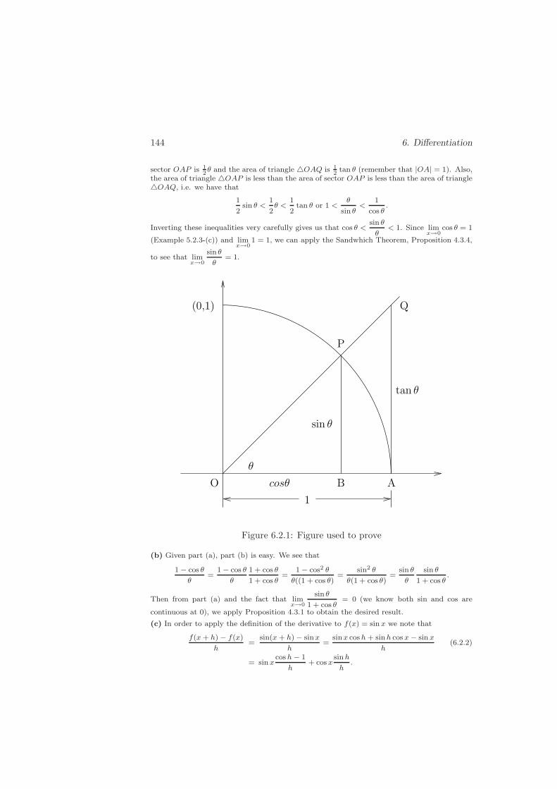
144 6. Differentiation
sector OAP is 12θ and the area of triangle △OAQ is 1
2tan θ (remember that |OA| = 1). Also,
the area of triangle △OAP is less than the area of sector OAP is less than the area of triangle△OAQ, i.e. we have that
1
2sin θ <
1
2θ <
1
2tan θ or 1 <
θ
sin θ<
1
cos θ.
Inverting these inequalities very carefully gives us that cos θ <sin θ
θ< 1. Since lim
x→0cos θ = 1
(Example 5.2.3-(c)) and limx→0
1 = 1, we can apply the Sandwhich Theorem, Proposition 4.3.4,
to see that limx→0
sin θ
θ= 1.
θ
B AO
P
Q(0,1)
sin θ
tan θ
cosθ
1
Figure 6.2.1: Figure used to prove
(b) Given part (a), part (b) is easy. We see that
1 − cos θ
θ=
1 − cos θ
θ
1 + cos θ
1 + cos θ=
1 − cos2 θ
θ((1 + cos θ)=
sin2 θ
θ(1 + cos θ)=
sin θ
θ
sin θ
1 + cos θ.
Then from part (a) and the fact that limx→0
sin θ
1 + cos θ= 0 (we know both sin and cos are
continuous at 0), we apply Proposition 4.3.1 to obtain the desired result.
(c) In order to apply the definition of the derivative to f(x) = sin x we note that
f(x + h) − f(x)
h=
sin(x + h) − sinx
h=
sinx cos h + sinh cos x − sin x
h(6.2.2)
= sin xcos h − 1
h+ cos x
sin h
h.

6.2 Some Derivatives 145
Then using parts (a) and (b) we get
f ′(x) = limh→0
f(x + h) − f(x)
h= lim
h→0
[
sinxcos h − 1
h+ cos x
sinh
h
]
= cos x.
Of course the derivatives of the rest of the trig functions follow from the deriva-tive of the sine function.
In Example 4.2.7 we showed that the limit of the function
f1(x) =
{
sin(
1x
)
if x 6= 0
0 if x = 0
does not exist at x = 0—hence we know that f1 is not continuous at x = 0—soit’s surely not differentiable at x = 0. In Example 5.2.4 we showed that the
function f2(x) =
{
x sin(
1x
)
if x 6= 0
0 if x = 0
is continuous at x = 0—thus it’s at least a candidate for differentiability. Wenext include the following example.
Example 6.2.4 (a) Show that f2 is not differentiable at x = 0.
(b) Show that the function f3 : R → R defined by f3(x) =
{
x2 sin(
1x
)
if x 6= 0
0 if x = 0
is differentiable at x = 0.
Solution: (a) We note that
limx→0
f2(x) − f2(0)
x − 0= lim
x→0sin
(
1
x
)
.
We know that this last limit does not exist—by the same approach that we used to show thatf1 was not continuous at x = 0. Therefore the derivative of f2 does not exist at x = 0.
(b) We start the same way that we started with part (a) and note that
limx→0
f3(x) − f3(0)
x − 0= lim
x→0x sin
(
1
x
)
.
We showed in Example 5.2.4 that this last limit exists and equals zero. Therefore f3 isdifferentiable at x = 0 and f ′
3(0) = 0.
You should view the functions f1, f2, and f3 as a series of functions, admittednot especially nice functions, that have obvious similarities. The function f2 issmoothed enough so that it is continuous at x = 0 (where f1 was not) butnot differentiable. The function f3 is smoothed more—it is differentiable atx = 0 and hence also continuous there. In addition, we should realize that allof the functions f1, f2 and f3 are differentiable when x 6= 0—if we knew how todifferentiate the sine function.
HW 6.2.1 Consider the function f(x) = x3 − 2x2 + x − 1 defined on R. (a)Use Definition 6.1.1 to compute f ′(2).(b) Compute f ′(x).
HW 6.2.2 Computed
dxx1/3.

146 6. Differentiation
HW 6.2.3 Compute limθ→0
sin 3θ
sin 5θ.
HW 6.2.4 Consider the function f(x) =
{
x2 if x ∈ [−1, 1] ∩ Q
−x2 if x ∈ [−1, 1] ∩ I.
(a) Is f differentiable at x ∈ [−1, 1], x 6= 0? If so, compute f ′(x).(b) Is f differentiable at x = 0? If so, compute f ′(0).
HW 6.2.5 We saw in Example 6.2.4 that f3 is differentiable at x = 0. (a)Show that f3 is differentiable for x 6= 0.(b) Determine where f ′
3 is continuous.
6.3 Some Differentiation Theorems
Now that we have some of the basic properties of the concept of the derivatve,it is time to develop some additional applications of differentiation. There aremany very important applications of differentiation and you have surely seensome of these in your basic course.
We begin with a very important result—but one we want now more as alemma. Recall that in Section 5.3 we defined maximums and minimums as themaximum and minimum in some neighborhood about a point—Definition 5.3.6(a) and (c). We begin with the very important result.
Proposition 6.3.1 Suppose the function f is such that f : (a, b) → R for somea, b ∈ R, a < b and suppose that f is differentiable at x0 ∈ (a, b). If f has amaximum or minimum at the point (x0, f(x0)), then f ′(x0) = 0.
Proof; Consider the case where (x0, f(x0)) is a maximum. Let N ⊂ (a, b) bea neighborhood of x0 so that f(x) ≤ f(x0) for all x ∈ N . (The definition of amaximum gives us a neighborhood. If we then intersect that neighborhood with(a, b), we get N . The neighborhood N will still be an interval and x0 ∈ N .)
Since limx→x0
f(x) − f(x0)
x− x0exists (f is differentiable at x0), by Proposition 4.4.8
both limx→x0−
f(x) − f(x0)
x− x0and lim
x→x0+
f(x) − f(x0)
x− x0exist and are equal. If x ∈ N
and x < x0, then x − x0 < 0, f(x) − f(x0) ≤ 0 and hencef(x) − f(x0)
x− x0≥ 0
(the slope is positive going up hill).
Claim 1: limx→x0−
f(x) − f(x0)
x− x0≥ 0: We prove this claim by contradiction. We
assume that limx→x0−
f(x) − f(x0)
x− x0< 0, i.e. there exists L < 0 such that for every
ǫ > 0 where exists δ such that 0 < x0 − x < δ implies
∣
∣
∣
∣
f(x) − f(x0)
x− x0− L
∣
∣
∣
∣
< ǫ.
Choose ǫ = |L|/2. Then there exists a δ such that 0 < x0 − x < δ implies
6.3 Differentiation Theorems 147
that∣
∣
∣
f(x)−f(x0)x−x0
− L∣
∣
∣< |L|/2 or − |L|/2 + L < f(x)−f(x0)
x−x0< |L|/2 + L or
f(x)−f(x0)x−x0
< −|L|/2.
This contradicts that fact thatf(x) − f(x0)
x− x0≥ 0 for x ∈ (x0 − δ, x0)∩N so
we know that limx→x0−
f(x) − f(x0)
x− x0≥ 0.
Claim 2: limx→x0+
f(x) − f(x0)
x− x0≤ 0: This proof is very much like the last case.
We show that if x ∈ N and x > x0, thenf(x) − f(x0)
x− x0≤ 0 (the slope is
negative going down hill). We then assume that limx→x0+
f(x) − f(x0)
x− x0> 0, apply
the definition of the right hand limit with ǫ = L/2 and arrive at a contradicition.
Therefore limx→x0+
f(x) − f(x0)
x− x0≤ 0.
Since limx→x0−
f(x) − f(x0)
x− x0≥ 0, lim
x→x0+
f(x) − f(x0)
x− x0≤ 0 and they are equal,
they both must be zero. Therefore the limit limx→x0
f(x) − f(x0)
x− x0= 0 or f ′(x0) =
0.We can prove the analogous result for a minimum using a completely similar
argument or by considering the function −f—if f has a minimum at x0, then−f will have a maximum at x0.
Of course we know that Proposition 6.3.1 gives us a powerful tool for findinglocal maximums and minimums. We set f ′(x) = 0—we called these pointscritical points in our basic course. This gives us all of the maximums andminimums at points at which f is differentiable and probably a few extras. Wethen develop methods (which we will develop later) to determine which of thesecritical points is actually a maximum or minimum. Then if we consider anypoints at which f is not differentiable and maybe some end points, we have themaximums and minimums.
However, at this time we wanted Proposition 6.3.1 to help us prove thefollowing theorem commonly referred to as Rolle’s Theorem.
Theorem 6.3.2 (Rolle’s Theorem) Suppose that f : [a, b] → R is continuouson [a, b], differentiable on (a, b) and such that f(a) = f(b). Then there exists aξ ∈ (a, b) such that f ′(ξ) = 0.
Proof: We know from Theorem 5.3.8 that there exists x0, y0 ∈ [a, b] such thatf(x0) = min{f(x) : x ∈ [a, b]} and f(y0) = max{f(x) : x ∈ [a, b]}. If both x0
and y0 are endpoints of [a, b] (and f(a) = f(b)), then f is constant on [a, b],f ′(x) = 0 for x ∈ (a, b) so we can choose ξ = a+ b/2. Otherwise, either x0 or y0is in (a, b), say x0 ∈ (a, b). Then by Proposition 6.3.1 we know that f ′(x0) = 0,i.e. we can set ξ = x0.
The real reason that we want Rolle’s Theorem is to help us prove the MeanValue Theorem, abbreviated by MVT, which is a very important result.

148 6. Differentiation
Theorem 6.3.3 (Mean Value Theorem (MVT) Suppose that f : [a, b] → R
is continuous on [a, b] and differentiable on (a, b). Then there exists a ξ ∈ (a, b)
such that f ′(ξ) =f(b) − f(a)
b− a.
Proof: The proof of this result is very easy to prove as long as we know the
”trick.” We set h(x) = f(x)−f(a)− f(b) − f(a)
b− a(x−a). Then h(a) = h(b) = 0, h
is continuous on [a, b] and h is differentiable on (a, b). Thus by Rolle’s Theorem,Theorem 6.3.2, there exists ξ ∈ (a, b) such that h′(ξ) = 0, i.e. h′(ξ) = f ′(ξ) −f(b) − f(a)
b− a= 0 which is what we were to prove.
Often the results of the Mean Value Theorem will be given in the formf(b) − f(a) = f ′(ξ)(b − a).
The Mean Value Theorem is important in the form given in Theorem 6.3.3but is most important for some of the very important corollaries that follow eas-ily from the theorem. We begin with two results that are related to integration—even thought at this time we don’t know what integration is.
Corollary 6.3.4 Suppose f : (a, b) → R is differentiable on (a, b) and such thatf ′(x) = 0 for x ∈ (a, b). Then f is constant on (a, b).
Proof: Choose any two values x0, y0 ∈ (a, b) where x0 6= y0, say x0 < y0.Since f is differentiable on (a, b) we know that f is differentiable on (x0, y0) andby Proposition 6.1.2 f is continuous on [x0, y0]. We can then apply the MVTand get f(y0) − f(x0) = f ′(ξ)(b − a) for ξ ∈ (x0, y0). Since f ′(x) = 0 for allx ∈ (a, b), f ′(ξ) = 0 and we have that f(x0) = f(y0). Since this is true for anyx0, y0 ∈ (a, b), f must be a constant on (a, b).
Corollary 6.3.5 Suppose f, g : (a, b) → R are such that f and g are differen-tiable on (a, b) and f ′(x) = g′(x) for all x ∈ (a, b). Then there exists a constantC ∈ R such that f(x) = g(x) + C for all x ∈ (a, b).
Proof: Define h by h(x) = f(x)− g(x). If we then apply Corollary 6.3.4 to thefunction h, we see that h is constant on (a, b). This is what we wanted to prove.
Do these for any open interval—include R and (0,∞)????As we stated earlier you should recall that you used both of the above results
often in your basic course. We next give the results that related increasing-decreasing functions with their derivatives. Recall that in Definition 5.4.3 wedefined increasing and decreasing, and strictly increasing and strictly decreasingfunctions. We state the following corollary.
Corollary 6.3.6 Suppose f : (a, b) → R is differentiable on (a, b). We thenhave the following results.(a) If f ′(x) > 0 for all x ∈ (a, b), then f is strictly increasing on (a, b).(b) If f ′(x) ≥ 0 for all x ∈ (a, b), then f is increasing on (a, b).
6.3 Differentiation Theorems 149
(c) If f ′(x) < 0 for all x ∈ (a, b), then f is strictly decreasing on (a, b).(d) If f ′(x) ≤ 0 for all x ∈ (a, b), then f is decreasing on (a, b).
Proof: (a) Suppose x, y ∈ (a, b) are such that x < y. Then f is differentiableon (x, y) and continuous on [x, y] so we can apply the MVT. We get f(y) −f(x) = f ′(ξ)(y − x) for ξ ∈ (x, y). Since f ′(ξ) > 0 and y − x > 0, we get thatf(y) − f(x) > 0, or f(x) < f(y), or f is strictly increasing.
The proofs of (b), (c) and (d) follow from the MVT in exactly the same way.
We should realize that the application of Corollary 6.3.6 along with Propo-sition 6.3.1 gives us a method for catorgorizing the maximums and minimumsof a function. We use Proposition 6.3.1 (along with listing the points where thederivative does not exist) to find the potential maximums and minimums, criti-cal points. We handle points at which the function is not defined separately. Wethen evaluate f ′ at one point in the interval between each of these critical pointsto determine whether f is strictly increasing or decreasing in that interval—ifwe have all critical points listed, the sign of f ′ cannot change in the interval.We then classify the critical point as a maximum if the curve of the functionis increasing to the left of the critical point and decreasing to the right of thecritical point. We classify the critical point as a minimum if the curve of thefunction is decreasing to the left of the critical point and increasing to the rightof the critical point.
Also we get a very useful result from Corollary 6.3.6. From Proposition 5.4.8we saw that if a function f is strictly monotone on the domain of the function,then the function was one-to-one. Then from Corollary 6.3.6 and Proposition5.4.8 we obtain the following useful result.
Corollary 6.3.7 Suppose f : (a, b) → R is differentiable on (a, b). We thenhave the following results.(a) If f ′(x) > 0 for all x ∈ (a, b), then f is one-to-one on (a, b).(b) If f ′(x) < 0 for all x ∈ (a, b), then f is one-to-one on (a, b).
We next return to the situation of inverse functions. In Section 5.4, Propo-sition 5.4.11 we proved that if I is an interval and f is either strictly monotoneon I or one-to-one and continuous on I, then f−1 is continuous on f(I). Wenext give the result that gives a differentiability condition for f−1.
Proposition 6.3.8 Suppose that f : I → R where I ⊂ R is an interval. Assumethat f is one-to-one and continuous on I. If x0 ∈ I is not an end point of I, fis differentiable at x = x0 and f ′(x0) 6= 0, then f−1 : f(I) → R is differentiableat y0 = f(x0) and
(
f−1)′
(y0) =1
f ′(x0). (6.3.1)
Proof: Read this proof carefully. It is a very technical proof. As discussedearlier we already know that f−1 is continuous on f(I).

150 6. Differentiation
We know that limx→x0
f(x) − f(x0)
x− x06= 0. Hence
1
f ′(x0)= limx→x0
1f(x)−f(x0)
x−x0
= limx→x0
x− x0
f(x) − f(x0).
Thus for every ǫ > 0 there exists δ such that 0 < |x− x0| < δ implies
∣
∣
∣
∣
x− x0
f(x) − f(x0)− 1
f ′(x0)
∣
∣
∣
∣
< ǫ. (6.3.2)
Let g = f−1. Since g is continuous at y0, for every ǫ1 > 0 there exists δ1such that 0 < |y − y0| < δ1 implies |g(y) − g(y0)| < ǫ1. Apply this continuityargument with ǫ1 = δ (from the preceeding paragraph) and call the given δ1 η,i.e. we have 0 < |y − y0| < η implies |g(y) − g(y0)| < δ.
Then 0 < |y− y0| < η implies |g(y)− g(y0)| < δ or |g(y)− x0| < δ. Then by
(6.3.2) implies that
∣
∣
∣
∣
g(y) − x0
f(g(y)) − f(x0)− 1
f ′(x0)
∣
∣
∣
∣
< ǫ (where the last expression
follows by replacing x in (6.3.2) by g(y)).Note that because x0 = g(y0), f(g(y)) = y and f(x0) = y0,
∣
∣
∣
∣
g(y) − x0
f(g(y)) − f(x0)− 1
f ′(x0)
∣
∣
∣
∣
=
∣
∣
∣
∣
g(y) − g(y0)
y − y0− 1
f ′(x0)
∣
∣
∣
∣
.
Therefore we have that for every ǫ > 0 there exists an η such that 0 < |y−y0| < η
implies
∣
∣
∣
∣
g(y) − g(y0)
y − y0− 1
f ′(x0)
∣
∣
∣
∣
< ǫ or limy→y0
g(y) − g(y0)
y − y0=
1
f ′(x0)—which is
what we were to prove.
We next give a nice application of Proposition 6.3.8. In Section 5.6 we usedProposition 5.4.8 to define y1/n, we used Proposition 5.4.11 to show that thefunction y1/n is continuous on [0,∞), and then used the composition of y1/n andxm to define xr, r ∈ Q and show that xr is continuous. We now want to extendthese results to show that xr is differentiable. To do so in the most pleasantway we return to Example 5.6.1 and consider
√y. (Recall that in Example 6.2.2
we proved thatd
dy
√y =
1
2√y. We did so using more elementary methods and
methods that did not extend as nicely to y1/n—and methods that weren’t asnice as these.)
Example 6.3.1 Consider the function f(x) = x2 on D = [0,∞). Show that f−1(y) =√
y
is differentiable on [0,∞) and thatd
dy
√y =
1
2√
y=
1
2y−1/2.
Solution: We should recall that we already know that f is invertible, that f−1 is continuouson [0,∞) and that f−1(y) =
√y. We see that it is very easy to apply Proposition 6.3.8 to
f—we know that f : I = [0,∞) → R, I is surely an interval and that f is one-to-one andcontinuous on I. We let y0 be an arbitrary element of [0,∞) and let x0 ∈ [0,∞) be suchthat y0 = f(x0) = x2
0, i.e. x0 =√
y0. Then we know from Proposition 6.3.8 that f−1 is
differentiable at y0 andd
dyf−1(y0) =
1
f ′(x0)=
1
2x0=
1
2√
y0. This is what we were to prove.
6.3 Differentiation Theorems 151
Of course we next extend the above result to the function y1/n.
Example 6.3.2 Consider the function f(x) = xn on D = [0,∞). Show that f−1(y) =
y1/n = n√
y is differentiable on [0,∞) and thatd
dyy1/n =
1
ny
1n−1.
Solution: We proceed exactly as we did in the previous example. We know from Section5.6 that f is invertible, that f−1 is continuous on [0,∞) and f−1(y) = y1/n. It is also easyto see that f satisfies the hypotheses of Proposition 6.3.8. Again let x0 ∈ D = [0,∞) and
y0 ∈ f(D) = [0,∞) be such that y0 = f(x0) = xn0 or x0 = y
1/n0 . Then by Proposition 6.3.8
we know that f−1 is differentiable for any y0 ∈ f(D) = [0,∞) and
d
dyf−1(y0) =
1
f ′(x0)=
1
nxn−10
=1
n(
y1/n0
)n−1=
1
ny1−1/n0
=1
ny
1n−1
which is what we were to prove.
Of course the next step is to apply the Chain Rule, Proposition 6.1.4 toprove that for r ∈ R, r = m/n,
d
dxxr =
d
dx
(
x1/n)m
= m(
x1/n)m−1 1
nx
1n−1 =
m
nx
m−1
n + 1n−1 = rxr−1.
This is important enough that we state this result in the form of a proposition.
Proposition 6.3.9 Consider r = mn ∈ Q and the function g : [0,∞) → R
defined by g(x) = xr. The function g is continuous and differentiable on [0,∞)and for any x0 ∈ [0,∞) we have g′(x0) = rxr−1
0 .
The inverse trig functions provide us with another nice application of thePropositions 5.4.11 and 6.3.8. In our basic functions course some time afterdefining the trig functions we defined the inverse trig functions—for the sinefunction, probably very intuitively as θ = sin−1 x as the ”angle whose sine isx.” The interesting part and sometimes the tough part is that the sine function isnot one-to-one. We can get around this problem easily. Suppose for the momentwe write sinx to denote the sine function defined on R and define the restrictionof sin to [−π/2, π/2] by Sin x—this is a temporary, uncommon notation used tomake the point. It should be reasonably clear that though sin is not one-to-one,Sin is one-to-one—we have restricted the domain, just as you did in your basiccourse, so as to make the restriction one-to-one. We then have the followingresult.
Example 6.3.3 Consider the function f = Sin : D = [−π/2, π/2] → R where f(x) =Sin x = sin x. Show that f−1 exists on f(D) = [−1, 1], f−1 is continuous on [−1, 1], f−1 is
differentiable on (−1, 1) and(
f−1)′
(x0) =1√
1 − x2for x0 ∈ (−1, 1).
Solution: Above we stated that it was ”reasonably clear” that Sin is one-to-one. We alsoneed to know that the Sin function is monotone. Since we know that d
dxsinx = cos x and
cos x > 0 on (−π/2, π/2), by Corollaries 6.3.6 and 6.3.7 we know that the Sin function isstrictly increasing and one-to-one on the interval (−π/2, π/2). Since we also know that thesine function does not equal ±1 on the open interval (−π/2, π/2), we can include the endpoints to see that the function Sin is strictly increasing and one-to-one on [−π/2, π/2].
Since f is monotone, we can apply Proposition 5.4.11 to see that f−1 is continuous onf(D) = [−1, 1]. We know from Example 5.2.3-(d) that the sine function is continuous on
152 6. Differentiation
R—hence f(x) = Sin x is continuous on D = [−π/2, π/2]. Then since we already knoiw thatf is one-to-one, by Proposition 6.3.8 f−1 = sin−1 is differentiable on f(D) = (−1, 1), and for
x ∈ (−1, 1) and θ ∈ [−π/2, π/2] such that sin θ = x, we haved
dxsin−1 x =
1
f ′(θ)=
1
cos θ.
We know that cos θ = ±√
1 − sin2 θ. Because for θ ∈ [−π/2, π/2] we know that cos θ ≥ 0, we
have cos θ =√
1 − sin2 θ. Also sin θ = x so we haved
dxsin−1 x =
1√1 − x2
—the formula you
learned in your basic course.
Of course we know that f−1 is usually written as sin−1. You should be carefulwith this notation. In some texts—usually old ones—they will write sin−1 asthe inverse of sin (not a function since sin is not one-to-one) and Arcsin as theinverse of Sin. This is nice notation because it emphasizes the fact that sinis not one-to-one but it doesn’t seem to be used much anymore. Just use thenotation sin−1 to denote the inverse of the Sin function and never talk aboutthe inverse of the sin function—because the inverse isn’t even a function. Butbe careful.
Also we should realize that we could next consider the cosine, tangent, se-cant, etc functions. Just like the sine function, none of these functions areone-to-one. Thus we restrict the domain as you did in your basic class (some-times different from the domain used to define sin−1 and proceed as we did inExample 6.3.3. We emphasize that having different domains for these functionscan make things difficult when we have the more than one of them interactingwith each other. Also we must be careful when using a calculator.
HW 6.3.1 (True or False and why) (a) Suppose f, g : (a, b) → R are such thatf and g are differentiable on (a, b), f ′(x) = g′(x) for x ∈ (a, b) and f((a+b)/2) =g((a+ b)/2). Then f(x) = g(x) for all x ∈ (a, b).(b) Suppose f : R → R is strictly increasing on R. Then f ′(x) > 0 for x ∈ R.(c) Suppose f : [−1, 1] → R has a maximum at x = 0. Then f ′(0) = 0.(d) The function f(x) = x+ sinx is strictly monotone on [0,∞).(e) Suppose f : (−3, 3) → R is differentiable on (−3, 3) and such that |f ′(x)| > 0on (−3, 3). Then f is strictly monotone on (−3, 3).
HW 6.3.2 Consider the function f(x) = |x| for x ∈ R. Show that if a < 0 < b,then there is no ξ ∈ (a, b) such that f(b) − f(a) = f ′(ξ)(b − a). Why does thisnot contradict the Mean Value Theorem.
HW 6.3.3 Consider the function f : R → R defined by f(x) = 2x− cosx. (a)Prove that f is invertible and f−1 is continuous on R.(b) Prove that f−1 is differentiable and find df
dx
∣
∣
x=−π/2.
HW 6.3.4 Suppose f : D → R, D ⊂ R, is differentiable on D and for some Msatisfies |f(x)| ≤M . Prove that f is uniformly continuous on D.
HW 6.3.5 Suppose f : [a, b] → R is continuous on [a, b] and differentiable on(a, b). Prove that if f ′(x) 6= 0 for all x ∈ (a, b), then f is one-to-one.
6.4 L’Hospital’s Rule 153
6.4 L’Hospital’s Rule
In Proposition 4.3.1-(f) we found that if f → L1, g → L2 and L2 6= 0, then
f/g → L1/L2. In Example 4.2.4 we found that limx→4
x3 − 64
x− 4= 48, i.e. we found
the limit of a quotient when the limit in the denominator is zero. We did thisby dividing out the x − 4 term in the numerator and the denominator. And
finally in Example 6.2.3 we proved that limθ→0
sin θ
θ= 1—another example where
the limit exists where the limit in the denominator is zero. This time we wereunable to divide out the θ term so that we had to work much harder to find thelimit and prove 1 is the correct limit.
In this section we introduce L’Hospital’s Rule—a method for finding certainlimits of quotients. We begin by introducing the easiest version—a version thatwill satisfy many of our needs.
Proposition 6.4.1 (L’Hospital’s Rule) Suppose f, g : I → R where I isan interval, x0 ∈ I, f(x0) = g(x0) = 0, f and g are differentiable at x0 andg′(x0) 6= 0. Then
limx→x0
f(x)
g(x)=f ′(x0)
g′(x0).
Proof: We note that for x ∈ I, x 6= x0, we have
f(x)
g(x)=f(x) − f(x0)
g(x) − g(x0)=
f(x)−f(x0)x−x0
g(x)−g(x0)x−x0
.
Then
limx→x0
f(x)
g(x)=
limx→x0
f(x)−f(x0)x−x0
limx→x0
g(x)−g(x0)x−x0
=f ′(x0)
g′(x0)
which is what we were to prove.
We note that this version of L’Hospital’s Rule is enough to find both of the
singular limits that we have considered in the past: limx→4
x3 − 64
x− 4, Example 4.2.4,
and limx→0
sin θ
θ, Example 6.2.3-(a). Also note that if you consider a simple limit
such as limx→1
3x+ 4
2x− 3= −7, and blindly apply L’Hospital’s Rule, we would get
that the limit is 32—the wrong answer. As is often the case you must be careful
that the functions involved satisfy the hypotheses. The functions f(x) = 3x+4and g(x) = 2x − 3 do not satisfy the hypotheses f(1) = 0 and g(1) = 0. Andfinally, note that if I is a closed interval and x0 is an endpoint, then we have aversion of L’Hospital’s Rule for one-sided derivatives.
There are more difficult versions of L’Hospital’s Rule—and at times there is aneed for these more difficult versions. We will include several of these differentversions of L’Hospital’s Theorem. We will prove several of these results and
154 6. Differentiation
state several without proof. These proofs will depend strongly on the CauchyMean Value Theorem—an generalization of the Mean Value Theorem, Theorem6.3.3.
Proposition 6.4.2 (Cauchy Mean Value Theorem (CMVT)) Supposef, g : [a, b] → R are continuous on [a, b], differentiable on (a, b) and g is suchthat g′(x) 6= 0 on (a, b). Then there exists ξ ∈ (a, b) such that
f(b) − f(a)
g(b) − g(a)=f ′(ξ)
g′(ξ).
Proof: We prove this theorem very much we proved the Mean Value Theorem—we use a trick and Rolle’s Theorem, Theorem 6.3.2. We define a function h by
h(x) = f(x) − mg(x) where m =f(b) − f(a)
g(b) − g(a). Then it is easy to see that
h(a) = h(b), h is continuous on [a, b] and h is differentiable on (a, b). Thus byRolle’s Theorem, Theorem 6.3.2, there exists ξ ∈ (a, b) such that h′(ξ) = 0.Since h′(x) = f ′(x) −mg′(x), we have the desired result.
We should note that if we wanted to pretend that we were discovering theproof, we could set h(x) = f(x)−mg(x) (without telling what m is) and choosem so that h(a) = h(b). It’s still a trick—but a nice trick. Also we should noticethat if we set g(x) = x, we get the Mean Value Theorem, Theorem 6.3.3. Forthis reason sometimes Proposition 6.4.2 will be referred to as the GeneralizedMean Value Theorem.
Before we move on to some of the versions of LHospital’s Rules, we want todiscuss a few ideas that we will use often. The first is that though we will usethe CMVT in each of our results, we will always use a contorted version of theproposition. We will always work with an x and y in our domain where y < x.Then for example in part (a) of Proposition 6.4.3, we use the fact that
f(x) − f(y)
g(x) − g(y)=
f(x)g(x) −
f(y)g(x)
1 − g(y)g(x)
(6.4.1)
and apply the CMVT to the left hand side. Equation (6.4.1) is easily seen tobe true by simplifying the right hand side.
We should also note that in our applications of the CMVT, it is always thecase that g(x) 6= g(y)—because we will always assume that g′(x) 6= 0 on ourinterval I, the Mean Value Theorem, Theorem 6.3.3, implies that g(x)− g(y) =g′(ξ)(x − y) for some ξ ∈ (y, x). Thus g(x) − g(y) 6= 0.
And finally another operation we will use often is the following. Again in part
(a) of Proposition 6.4.3 we will have
∣
∣
∣
∣
∣
∣
f(x)g(x) −
f(y)g(x)
1 − g(y)g(x)
−A
∣
∣
∣
∣
∣
∣
< ǫ where x is fixed and
f and g approach zero as y → c+. We let y → c+ and get
∣
∣
∣
∣
∣
∣
f(x)g(x) − 0
1 − 0−A
∣
∣
∣
∣
∣
∣
≤ ǫ.
We should realize that this follows from HW4.1.4.

6.4 L’Hospital’s Rule 155
Since some flavor of each of the above statements will appear in each proof,we thought that we’d belabor the idea once and in the proofs just proceed as ifwe know what we’re doing. Thus we begin with the following result where weconsider several of the possibilities when x is approaching a real number fromthe right hand side.
Proposition 6.4.3 (L’Hospital’s Rule) Suppose that f, g : I = (c, a) → R,c, a ∈ R, where f, g are differentiable on I and g is assumed to satisfy g(x) 6= 0,g′(x) 6= 0 on I. We then have the following results.
(a) If limx→c+
f(x) = limx→c+
g(x) = 0 and limx→c+
f ′(x)
g′(x)= A ∈ R, then lim
x→c+
f(x)
g(x)=
A.
(b) If limx→c+
f(x) = limx→c+
g(x) = 0 and limx→c+
f ′(x)
g′(x)= ∞, then lim
x→c+
f(x)
g(x)= ∞.
(c) If limx→c+
g(x) = ∞ and limx→c+
f ′(x)
g′(x)= A ∈ R, then lim
x→c+
f(x)
g(x)= A.
(d) If limx→c+
g(x) = ∞ and limx→c+
f ′(x)
g′(x)= ∞, then lim
x→c+
f(x)
g(x)= ∞.
Proof: (a) Suppose ǫ > 0 is given and let ǫ1 = ǫ/2. Since limx→c+
f ′(x)
g′(x)= A,
for ǫ1 given we know that there exists a δ such that ξ ∈ (c, c + δ) implies that∣
∣
∣
∣
f ′(ξ)
g′(ξ)−A
∣
∣
∣
∣
< ǫ1. Choose x, y ∈ (c, c + δ) such that y < x. By the CMVT
there exists ξy ∈ (y, x) such thatf(x) − f(y)
g(x) − g(y)=f ′(ξy)
g′(ξy). Note that ξy is also in
(c, c+ δ). Then
∣
∣
∣
∣
∣
∣
f(x)g(x) −
f(y)g(x)
1 − g(y)g(x)
−A
∣
∣
∣
∣
∣
∣
=
∣
∣
∣
∣
f(x) − f(y)
g(x) − g(y)−A
∣
∣
∣
∣
=
∣
∣
∣
∣
f ′(ξy)
g′(ξy)−A
∣
∣
∣
∣
< ǫ1.
We then let y → c+, noting that ξy ∈ (c, c + δ) for all of the y’s, and get∣
∣
∣
f(x)g(x) −A
∣
∣
∣≤ ǫ1 = ǫ/2 < ǫ for any x ∈ (c, c+ δ). Therefore lim
x→c+
f(x)
g(x)= A.
You might notice that this proof isn’t too different from the proof of Propo-sition 6.4.1, except in this case since we cannot evaluate f or g at x = c, we usex and y and then let y → c+. Otherwise the proofs are really very similar.
(b) Suppose K > 0 is given—this time we are proving that a limit is infinite so
we begin with K in place of the traditional ǫ. Let K1 = 2K. Since limx→c+
f ′(x)
g′(x)=
∞, there exists a δ such that ξ ∈ (c, c + δ) implies thatf ′(ξ)
g′(ξ)> K1. Choose
x, y ∈ (c, c + δ) with y < x. By the CMVT there exists ξy ∈ (y, x) such that

156 6. Differentiation
f(x) − f(y)
g(x) − g(y)=f ′(ξy)
g′(ξy). Then we have
f(x)g(x) −
f(y)g(x)
1 − g(y)g(x)
=f(x) − f(y)
g(x) − g(y)=f ′(ξy)
g′(ξy)> K1
—since ξy ∈ (y, x) ⊂ (c, c+ δ)—and it’s true for any y and ξy as long as y < x.
Let y → c+ and getf(x)
g(x)≥ K1 = 2K > K for all x ∈ (c, c + δ). Thus
limx→c+
f(x)
g(x)= ∞.
(c) The proof of statement (c) is difficult. We feel that it is important for youto know that there is a rigorous proof. We also feel that it is important thatyou are able to read and understand such a proof—even when it is tough. Weproceed.
Suppose ǫ > 0 is given. Let ǫ1 = min{1, ǫ/2}. Since limx→c+
f ′(x)
g′(x)= A, for
ǫ1 > 0 given, there exists δ1 such that ξ ∈ (c, c + δ1) implies
∣
∣
∣
∣
f ′(ξ)
g′(ξ)−A
∣
∣
∣
∣
< ǫ1.
Choose x, y ∈ I such that y < x < c+ δ. Then since ξy ∈ (y, x) ⊂ (c, c+ δ1)∣
∣
∣
∣
∣
∣
f(y)g(y) −
f(x)g(y)
1 − g(x)g(y)
−A
∣
∣
∣
∣
∣
∣
=
∣
∣
∣
∣
f(y) − f(x)
g(y) − g(x)−A
∣
∣
∣
∣
=
∣
∣
∣
∣
f ′(ξy)
g′(ξy)−A
∣
∣
∣
∣
< ǫ1. (6.4.2)
Since limy→c+
g(y) = ∞ for a fixed x there exists δ4 such that y ∈ (c, c + δ4)
implies that 1 − g(x)
g(y)> 0. Set ǫ2 = ǫ1/2[2 + |A|]. Again using the fact that
limy→c+
g(y) = ∞, there exists δ5 such that y ∈ (c, c+δ5) implies that g(y) >|f(x)|ǫ2
and there exists δ6 such that y ∈ (c, c + δ6) implies that g(y) >|g(x)|ǫ2
. Let
δ = min{δ4, δ5, δ6}. Then y ∈ (c, c+ δx) implies that |f(x)|g(y) < ǫ2 and |g(x)|
g(y) < ǫ2.
Now from (6.4.2) we have
−ǫ1 +A <
f(y)g(y) −
f(x)g(y)
1 − g(x)g(y)
< A+ ǫ1
or
(−ǫ1 +A)
(
1 − g(x)
g(y)
)
+f(x)
g(y)<f(y)
g(y)< (ǫ1 +A)
(
1 − g(x)
g(y)
)
+f(x)
g(y). (6.4.3)
Note that|g(x)|g(y)
< ǫ2 implies that −ǫ2 <g(x)
g(y)< ǫ2. From this we see that
1 − g(x)
g(y)> 1 − ǫ2 and 1 − g(x)
g(y)< 1 + ǫ2. Also, |f(x)|
g(y) < ǫ2 implies that
6.4 L’Hospital’s Rule 157
−ǫ2 < f(x)g(y) < ǫ2. Then inequality (6.4.3) gives
(−ǫ1 +A)(1 − ǫ2) − ǫ2 <f(y)
g(y)< (ǫ1 +A)(1 + ǫ2) + ǫ2
or
−ǫ1 +A− ǫ2(1 +A− ǫ1) <f(y)
g(y)< ǫ1 +A+ ǫ2(1 +A+ ǫ1). (6.4.4)
Using the fact that ǫ2 = ǫ1/2[2 + |A|] and the fact that ǫ1 ≤ 1, the extra termon the right hand side of (6.4.4) becomes
ǫ2(1 +A+ ǫ1) ≤ ǫ2(2 +A) ≤ ǫ2[2 + |A|] = ǫ1/2 < ǫ1.
The extra term on the left side of (6.4.4) (without the minus sign) becomes
ǫ2(1 +A− ǫ1) < ǫ2[1 +A] ≤ ǫ2[1 + |A|] =ǫ12
1 + |A|2 + |A| ≤
ǫ12< ǫ1.
These allow us to write inequality (6.4.4) as −ǫ + A < −2ǫ1 + A <f(y)
g(y)<
2ǫ1 + A < ǫ+A or
∣
∣
∣
∣
f(y)
g(y)−A
∣
∣
∣
∣
< ǫ for all y ∈ (c, c+ δ). Thus limy→c+
f(y)
g(y)= A.
(d) Let K > 0 be given. Let K1 = 2K + 1. Since limx→c+
f ′(x)
g′(x)= ∞, there exists
a δ1 such that ξ ∈ (c, c = δ1) implies thatf ′(ξ)
g′(ξ)> K1. Choose x, y ∈ (c, c+ δ1)
such that y < x. Then by the CMVT there exists ξy ∈ (y, x) such that
f(y)g(y) −
f(x)g(y)
1 − g(x)g(y)
=f(x) − f(y)
g(x) − g(y)=f ′(ξy)
g′(ξy)> K1. (6.4.5)
As in the proof of part (c) choose δ7 ( δ5 and δ6)|g(x)|g(y < 1
2 (which implies that32 > 1 − g(x)
g(y) >12 and |f(x)|
g(y) < 12 (which implies that − 1
2 < f(x)g(y) <
12 ). Then
inequality (6.4.5) gives
f(y)
g(y)>
(
1 − g(x)
g(y)
)
K1 +f(x)
g(y)>
1
2K1 −
1
2=
1
2(2K + 1) − 1
2= K
for all y ∈ (c, c+ δ7). Therefore limy→c+
f(y)
g(y)= ∞.
We next state and do not prove a version of l’Hospital’s Rule when x ap-proaches−∞. Originally we had included the proofs in the text but then decidedthat it did no good to include these proofs if no one reads them. They are tough.If you are interested in the proof see Advanced Calculus, Robert C. James.

158 6. Differentiation
Proposition 6.4.4 (L’Hospital’s Rule) Suppose that f, g : I = (−∞, a) →R, a ∈ R, where f, g are differentiable on I and g is assumed to satisfy g(x) 6= 0,g′(x) 6= 0 on I. We then have the following results.
(a) If limx→−∞
f(x) = limx→−∞
g(x) = 0 and limx→−∞
f ′(x)
g′(x)= A ∈ R, then lim
x→−∞f(x)
g(x)=
A.
(b) If limx→−∞
f(x) = limx→−∞
g(x) = 0 and limx→−∞
f ′(x)
g′(x)= ∞, then lim
x→−∞f(x)
g(x)=
∞.
(c) If limx→−∞
g(x) = ∞ and limx→−∞
f ′(x)
g′(x)= A ∈ R, then lim
x→−∞f(x)
g(x)= A.
(d) If limx→−∞
g(x) = ∞ and limx→−∞
f ′(x)
g′(x)= ∞, then lim
x→−∞f(x)
g(x)= ∞.

Chapter 7
Integration
7.1 An Introduction to Integration: Upper and
Lower Sums
The concept of the integral is very important. An integral is an abstract wayto perform a summation. We know of its application to areas, work, distance-velocity-acceleration, and much, much more. Generally the treatment of in-tegration given in the basic course is less than adequate—integration is moredifficult than differentiation and continuity. In this chapter we introduce theconcept of the integral and develop basic results concerning integration. Specif-ically, in this section we will lay the ground work for the definition. When wefeel that we want motivation for the integral, we will use the fact that we wantthe integral to represent the area under a given curve—hence in this section wewill give upper and lower approximations of the area in terms of sums.
Consider an interval [a, b] where a < b, and for n ∈ N consider P ={x0, · · · , xn} where a = x0 < x1 < · · · < xn−1 < xn = b. P is called a partitionof [a, b]. The points xi, i = 0, · · · , n, are called partition points. The intervals[xi−1, xi], i = 1, · · · , n, are called partition intervals. Note that P = {a, b} isthe most trivial partition of [a, b]. We we write a partition of [a, b], we will writethe partition as P = {x0, x1, · · · , xn}, assuming that we all know that x0 = a,xn = b and xi−1 < xi, for i = 1, · · · , n.
Definition 7.1.1 Consider the function f : [a, b] → R where f is bounded on[a, b], and P is a partition of [a, b], P = {x0, x1, · · · , xn}.(a) For each i, i = 1, · · · , n, define mi = glb{f(x) : x ∈ [xi−1, xi]} and Mi =lub{f(x) : x ∈ [xi−1, xi]}. (Note that these glb’s and lub’s exist because f isbounded on [a, b].)
(b) Define L(f, P ) =
n∑
i=1
mi(xi − xi−1) and U(f, P ) =
n∑
i=1
Mi(xi − xi−1).
159

160 7. Integration
The values L(f, P ) and U(f, P ) are called the lower and upper Darboux sumsof f based on P , respectively, or just the lower and upper sums.
We notice in Figure 7.1.1 that for the given partition P , L(f, P ) (repre-sented by the area under the thin horizontal lines) gives a lower approximationfor the area under the curve y = f(x), a ≤ x ≤ b, and U(f, P ) (represented bythe area under the thick horizontal lines) gives an upper approximation for thearea under the curve y = f(x), a ≤ x ≤ b. Note that when we use the word”approximation”, we do not mean that it necessarily provides an accurate ap-proximation. You should realize that if we include more points in the partition,the values L(f, P ) and U(f, P ) will provide better approximations of the areacompared the parition pictured—add a point to the partition in the figure, drawthe new version of the segments indicating the new upper and lower sums, andnote that the new upper and lower sums gives a value closer to the area underthe curve y = f(x).
x6a b
y = f(x)
x0
x1
x7x2
x3
x4
x5
Figure 7.1.1: Plot of the function y = f(x) on [a, b], a partition indicated on[a, b] and the step function representing the upper and lower sums, U(f, P ) andL(f, P ), respectively.
Consider the following examples.
Example 7.1.1 Let f1 denote the constant function f1(x) = k for x ∈ [a, b]. Let P ={x0, x1, · · · , xn} be a partition of [a, b]. Compute L(f1, P ) and U(f1, P ).
Solution: Let [xi−1, xi] denote one of the partition intervals associated with partition P . Itshould be clear that mi = glb{f1(x) : x ∈ [xi−1, xi]} = k and Mi = k. Then
L(f1, P ) =
n∑
i=1
mi(xi − xi−1) = k
n∑
i=1
(xi − xi−1) = k(b − a).
Also
U(f1, P ) =n∑
i=1
Mi(xi − xi−1) = kn∑
i=1
(xi − xi−1) = k(b − a).

7.1 Upper and Lower Sums 161
Example 7.1.2 Consider the function f2 : [0, 1] → R defined by f2(x) =
{
1 if x ∈ Q ∩ [0, 1]
0 if x ∈ I ∩ [0, 1]
and let P = {x0, · · · , xn} be a partition of [0, 1]. Compute L(f2, P ) and U(f2, P ).
Proof: Recall that f2 is the same function considered in Example 5.2.5. Let [xi−1, xi] denotea partition interval of partition P and assume that xi−1 < xi. Technically we could allowpoints xi−1 and xi be two points of a parition and have xi−1 = xi—but the partition interval[xi−1, xi] would contribute nothing to either L(f2, P ) or U(f2, P )—so why include such apoint. Since by Proposition 1.5.6-(a) there exists a q ∈ Q such that q ∈ (xi−1, xi), we see thatMi = 1. Also since by Proposition 1.5.6-(b) there exists p ∈ (xi−1, xi) such that p ∈ I, we seethat mi = 0. This is true for every i, i = 1, · · · , k. Thus
L(f2, P ) =n∑
i=1
mi(xi − xi−1) =n∑
i=1
0(xi − xi−1) = 0
and
U(f2, P ) =n∑
i=1
Mi(xi − xi−1) =n∑
i=1
1(xi − xi−1) = 1.
Example 7.1.3 Consider f3 : [0, 1] → R defined by f3(x) = 2x + 3 and the partition of[0, 1], P = {x0, · · · , xn}. Compute L(f3, P ) and U(f3, P ).
Proof: Since f3 is increasing, it is easy to that on the partition interval [xi−1, xi], mi =2xi−1 + 3 and Mi = 2xi + 3, i = 1, · · · , n. Thus
L(f3, P ) =n∑
i=1
mi(xi − xi−1) =n∑
i=1
(2xi−1 + 3)(xi − xi−1) = 2n∑
i=1
xixi−1 − 2n∑
i=1
x2i−1 + 3,
and
U(f3, P ) =n∑
i=1
Mi(xi − xi−1) =n∑
i=1
(2xi + 3)(xi − xi−1) = 2n∑
i=1
x2i − 2
n∑
i=1
xixi−1 + 3.
This is not very nice—and there’s no way to make it nice.
If instead we choose the partition P1 = {0, 1/n, 2/n, · · · , n/n = 1}, we get
L(f3, P1) =n∑
i=1
mi(xi − xi−1) =n∑
i=1
(
2i − 1
n+ 3
) (
i
n− i − 1
n
)
=2
n2
n∑
i=1
(i − 1) + 3 =2
n2
n(n − 1)
2+ 3
and
U(f3, P1) =n∑
i=1
mi(xi − xi−1) =
(
2i
n+ 3
) (
i
n− i − 1
n
)
=2
n2
n∑
i=1
i + 3 =2
n2
n(n + 1)
2+ 3.
These are much nicer expressions. You’d think they’d be useful for something—but rememberthat this is a very nice and specific partition.
We now proceed to develop some results comparing and relating the upperand lower sums. Because it is clear that mi ≤ Mi, i = 1, · · · , n, we obtain thefollowing result.
Proposition 7.1.2 Suppose f : [a, b] → R where f is bounded on [a, b] and Pis a partition of [a, b]. Then L(f, P ) ≤ U(f, P ).

162 7. Integration
Remember that we want∫ b
af to give us the area under the curve. If we look at
Figure 7.1.1 again, we note that for that to be true we at least must define∫ b
a f
so that for any partition P , L(f, P ) ≤∫ b
af ≤ U(f, P ), i.e. we must squeeze
∫ b
a f between the inequality given in Proposition 7.1.2.We next state and prove an easy but necessary lemma for our later work.
Lemma 7.1.3 Suppose that f : [a, b] → R is bounded such that m ≤ f(x) ≤Mfor all x ∈ [a, b]. Then for any partition P of [a, b], m(b − a) ≤ L(f, P ) andU(f, P ) ≤M(b− a).
Proof: Let the partition P be given by P = {x0, · · · , xn}. Since m ≤ f(x) forall x ∈ [a, b], surely m ≤ mi = glb{f(x) : x ∈ [xi−1, xi]} for all i, i = 1, · · · , n.Then
m(b− a) = m
n∑
i=1
(xi− xi−1) =
n∑
i=1
m(xi− xi−1) ≤n∑
i=1
mi(xi− xi−1) = L(f, P ),
which is one of the inequalities that we were to prove. The other inequalityfollows in the same manner.
One of the problems that we have is that we have defined the upper andlower Darboux sums for a particular partition. We have already discussed thefact that if we make the partition finer, the upper and lower sums give us better
approximations of the area—the value that we want for∫ b
a f . We must haveways to connect the sums in some way for different partitions. The next fewdefinitions and propositions do this job for us. We begin with the followingdefinition.
Definition 7.1.4 Let P and P ∗ be partitions of [a, b] given by P = {x0, · · · , xn}and P ∗ = {y0, · · · , ym}. If P ⊂ P ∗, then P ∗ is said to be a refinement of P .
Note that since the partitions P and P ∗ (and any other partitions that we maydefine) are given as a set of points in [a, b], the set containment definition abovemakes sense.
We should note that the easiest way to get a simple refinement of the parti-tion P is to add one point, i.e. if P = {x0, · · · , xn}, choose a point yI ∈ [xI−1, xI ]and let P ∗ = {x0, · · · , xI−1, yI , xI , · · · , xn}. We should then realize that if P ∗
is a refinement of the partition P , it is possible to consider a series of one-pointrefinements P0, · · · , Pk such that P0 = P , Pk = P ∗ and Pj is a one-point refine-ment of Pj−1 for j = 1, · · · , k. The construction consists of choosing P0 = Pand adding one of the points of P ∗−P = {x : x ∈ P ∗ and x 6∈ P} at each step.This observation makes several of the proofs given below much easier.
We next prove two lemmas, the first that relates the upper and lower sumson a partition and refinements of that partition and the second that relates thelower sum and upper sums with respect to different partitions.
Lemma 7.1.5 Suppose f : [a, b] → R where f is bounded on [a, b], P is apartition of [a, b] and P ∗ is a refinement of P . Then L(f, P ) ≤ L(f, P ∗) andU(f, P ∗) ≤ U(f, P ).

7.1 Upper and Lower Sums 163
Proof: Let P# be a one-point refinement of the partition P where P ={x0, · · · , xn} and the extra point in P#, yi is such that xi−1 ≤ yi ≤ xi. Thento compare L(f, P ) and L(f, P#) we only need to compare the contributions toboth of these values from the interval [xi−1, xi]. The contribution of this intervalto L(f, P ) is the value mi(xi−xi−1) where mi = glb{f(x) : x ∈ [xi−1, xi]}. Thecontribution of this same interval to L(f, P#) is the valuem1(yi−xi−1)+m
2(xi−yi) where m1 = glb{f(x) : x ∈ [xi−1, yi]} and m2 = glb{f(x) : x ∈ [yi, xi]}. Ofcourse we note that xi − xi−1 = (yi − xi−1) + (xi − yi).
We make the claim that m1 ≥ mi and m2 ≥ mi. To see that this is truewe note that since {f(x) : x ∈ [xi−1, yi]} ⊂ {f(x) : x ∈ [xi−1, xi]}, mi =glb{f(x) : x ∈ [xi−1, xi]} will be a lower bound of {f(x) : x ∈ [xi−1, yi]}. Hencemi ≤ f(x) for all x ∈ [xi−1, yi]} and thus mi ≤ m1 = glb{f(x) : x ∈ [xi−1, yi]},which also follows from HW1.4.1-(c). The fact that m2 ≥ mi follows in thesame manner.
Thus
mi(xi − xi−1) = mi [(yi − xi−1) + (xi − yi)]
= mi(yi − xi−1) +mi(xi − yi) ≤ m1(yi − xi−1) +m2(xi − yi),
so L(f, P ) ≤ L(f, P#).Now if P ∗ is any refinement of the partition P , from the discussion given pre-
ceeding this lemma we know that there exist one-point refinements P0, · · · , Pksuch that P0 = P , Pk = P ∗ and Pj is a one-point refinement of Pj−1 forj = 1, · · · , k. Thus by taking k steps involving the one-point refinement ar-gument given above (really an easy proof by induction) we see that L(f, P ) =L(f, P0) ≤ L(f, P1) ≤ · · ·L(f, Pk) = L(f, P ∗) which is what we were to prove.
The proof that U(f, P ∗) ≤ U(f, P ) is very similar. Using the one-pointpartition of P , P#, used above, the key step in the one-point partition argumentfor U is that
Mi = lub{f(x) : x ∈ [xi−1, xi]} ≥M1 = lub{f(x) : x ∈ [xi−1, yi]}
and
Mi = lub{f(x) : x ∈ [xi−1, xi]} ≥M2 = lub{f(x) : x ∈ [yi, xi]},
which follow from HW1.4.1-(c). The desired result then follows.
Lemma 7.1.6 Suppose that f : [a, b] → R where f is bounded on [a, b], andsuppose that P1 and P2 are partitions of [a, b]. Then L(f, P1) ≤ U(f, P2).
Proof: Let P ∗ be any common refinement of P1 and P2, i.e. P ∗ is a refinementof P1 and P ∗ is a refinement of P2. The smallest such common refinement isfound by setting P ∗ = P1 ∪ P2. Then by Lemma 7.1.5 we have L(f, P1) ≤L(f, P ∗) and U(f, P ∗) ≤ U(f, P2). By Proposition 7.1.2 we have L(f, P ∗) ≤U(f, P ∗). Thus we have
L(f, P1) ≤ L(f, P ∗) ≤ U(f, P ∗) ≤ U(f, P2).

164 7. Integration
If we return to Examples 7.1.1, 7.1.2 and 7.1.3, it’s really easy to see f1and f2 satisfy L(fj, P ) ≤ U(fj, P ) for j = 1, 2. It’s more difficult to see thatProposition 7.1.2 is satisfied for f3—but it is true because xi−1(xi − xi−1) ≤xi(xi − xi−1) (sum both sides of the inequality and add 3). Because the upperand lower sums for the functions f1 and f2 are so trivial, it is easy to see thatf1 and f2 will satisfy Lemma 7.1.5 for any refinement. Again because the upperand lower sums for f3 are so difficult, it is difficult to see that f3 will satisfyLemma 7.1.5—except by approximately reproducing the proof of Lemma 7.1.5with respect the function f3 and some particular refined partition. And finally,while it is again easy to see that functions f1 and f2 will satisfy Lemma 7.1.6with respect to any two partitions, it is very difficult to see that the upper andlower sums of the function f3 with respect to the partitions P and P1 will satisfyLemma 7.1.6. It should be clear that if we were to consider upper and lowersums for more complex functions, it would be next to impossible to comparethese upper and lower sums—especially with respect to very complex differentpartitions. It is for that reason that the above lemmas are so important.
HW 7.1.1 Consider the function f(x) = x and the partition of [0, 1], Pn ={0, 1
n ,2n , · · · , 1}. (a) Compute L(f, P ) and U(f, P .
(b) Compute U(f, Pn) − L(f, Pn).(c) Show that U(f, Pn) − L(f, Pn) > 0.(d) Compute lim
n→∞[U(f, Pn) − L(f, Pn)].
HW 7.1.2 Consider the function f(x) =
{
x if x ∈ Q ∩ [0, 1]
0 if x ∈ I ∩ [0, 1]
and the partition of [0, 1] Pn = {0, 1n ,
2n , · · · , 1}. (a) Compute L(f, Pn) and
U(f, Pn).(b) Compute U(f, Pn) − L(f, Pn) and lim
n→∞[U(f, Pn) − L(f, Pn)].
7.2 The Darboux Integral
In the last section we computed upper and lower Darboux sums that gave usapproximations of the area under the curve from above and below, respectively.If these sums weren’t so terrible to work with, we could live with them—that’sapproximately what they do numerically. However, the upper and lower sumsare not a very nice analytic tool—and we can do better—much better. In thefollowing definition we use the upper and lower sums to get a step nearer to thearea under the curve.
Definition 7.2.1 Consider f : [a, b] → R where f is bounded on [a, b]. (a) Wedefine the lower integral of f on [a, b] to be
∫ b
a
f = lub{L(f, P ) : P is a partition of [a, b]}.

7.2 The Integral 165
(b) We define the upper integral of f on [a, b] to be
∫ b
a
f = glb{U(f, P ) : P is a partition of [a, b]}.
We first note that if P ∗ is any fixed partition of [a, b], then by Lemma 7.1.6L(f, P ) ≤ U(f, P ∗) for any partition P . Because U(f, P ∗) is an upper boundfor the set {L(f, P ) : P is a partition of [a, b]} we know that lub{L(f, P ) :P is a partition of [a, b]} exists. Likewise, L(f, P ∗) is a lower bound of the set{U(f, P ) : P is a partition of [a, b]} so that glb{U(f, P ) : P is a partition of [a, b]}exists.
If we again return to Example 7.1.1, we see that since L(f1, P ) = U(f1, P ) =
k(b − a) for any partition P . Thus
∫ b
a
f1 =
∫ b
a
f1 = k(b − a). If we consider
the function f2 introduced in Example 7.1.2, we see that since L(f2, P ) = 0 for
any partition P ,
∫ 1
0
f2 = 0 and since U(f2, P ) = 1 for any partition P ,
∫ 1
0
f2 =
1. And finally, it should be reasonably easy to see that since L(f3, P ) andU(f3, P ) from Example 7.1.3 are so complex, it is too difficult to try to use these
expressions to determine
∫ 1
0
f3 or
∫ 1
0
f3. Even though L(f3, P1) and U(f3, P1)
found in Example 7.1.3 are much nicer, the lub and the glb in Definition 7.2.1above must be taken over all partitions of [0, 1], not just a few nice ones—so
knowing L(f, P1) and U(f, P1) does not help us determine
∫ 1
0
f3 or
∫ 1
0
f3 (at
least at this time).We see by Lemma 7.1.5 that as we add points to a partition, the upper sums
get smaller. We define
∫ b
a
f to be the glb of these upper sums. Likewise we
know that as we add points to a partition, the lower sums get larger. The lower
integral∫ b
af is defined to be the lub of these lower sums. Hence,
∫ b
af and
∫ b
af
squeeze in to provide a better upper and lower approximation of the area underthe curve y = f(x) from a to b, respectively.
We next prove a result that our intuition should tell us is obvious.
Proposition 7.2.2 Suppose that f : [a, b] → R, f is bounded on [a, b] and let
P be any partition of [a, b]. Then L(f, P ) ≤∫ b
a
f ≤∫ b
a
f ≤ U(f, P ).
Proof: The first inequality and the last inequality follow from the fact that thelub and the glb must be an lower bound and a upper bound of the set of allpossible sums, respectively.
Let P1 and P2 be any two partitions of [a, b]. By Lemma 7.1.6 we know thatL(f, P2) ≤ U(f, P1). Hence U(f, P1) is an upper bound of the set {L(f, P2) :

166 7. Integration
P2 is a partition of [a, b]}. Therefore
∫ b
a
f = lub{L(f, P2) : P2 is a partition of [a, b]} ≤ U(f, P1).
Then
∫ b
a
f is a lower bound of the set {U(f, P1) : P1 is a partition of [a, b]}.
Therefore
∫ b
a
f ≤ glb{U(f, P1) : P1 is a partition of [a, b]} =
∫ b
a
f which is
what we were to prove.
The upper sums U(f, P ) and the upper integral
∫ b
a
f approximate the area
under the curve y = f(x) from above, and the lower sums L(f, P ) and the
lower integral
∫ b
a
f approximate the area under the curve y = f(x) from below.
Since we want the integral
∫ b
a
f to give the area under the curve y = f(x), it is
reasonably logical to make the following definition.
Definition 7.2.3 Suppose f : [a, b] → R and f is bounded on [a, b]. We say
that f is integrable on [a, b] if
∫ b
a
f =
∫ b
a
f . If f is integrable on [a, b], we write
∫ b
a
f =
∫ b
a
f(
or
∫ b
a
f =
∫ b
a
f)
.
We call
∫ b
a
f the Darboux integral of f from a to b. We will actually drop
the Darboux from here on and refer to
∫ b
a
f as the integral of f from a to
b. We want to make it clear that this is the same integral that you studiedin your basic class. We tacked on the ”Darboux” to differentiate it from the”Riemann” integral that we define in Section 7.6—at which time we immediatelyprove that the Riemann and the Darboux integrals are the same. We use theDarboux definition because it makes some of the proofs easier and because wefeel that it is very intuitive.
Before we discuss the integral we want to emphasize that while we denote the
integral of f from a to b by∫ b
af , the most common notation (especially in the
basic course) is to denote the integral by∫ b
a f(x) dx. There are some advantagesto this latter notation. The ”dx” sort of reminds us that there is an xi−xi−1 inthe definition of the upper and lower sums. Also, later when we want to makea change of variables, the ”dx” term is very useful for reminding us what we
want to do. The notation∫ b
a f(x) dx can also be difficult to understand whenwe study differentials. In our basic course we had a ”dx” in the integral, a ”dx”

7.2 The Integral 167
as a part of differentials, with apparently no connection. In any case we will
generally use the notation∫ b
af to denote the integral of f from a to b—though
whenever it seems convenient or more clear to use the∫ b
af(x) dx notation, we
will use it.We return to the statement made just before we gave the definition of the
integral, ”it is reasonably logical to make the following definition.” It wouldn’t
be a good definition if it were always the case that
∫ b
a
f <
∫ b
a
f—then no
function would be integrable. It is only a good definition—and then our logic isaffirmed—if for a large set of nice functions, we can in fact get equality—and forsome functions we do not get equality. For a first glimpse of what we have, wereturn to our Examples 7.1.1, 7.1.2 and 7.1.3 from Section 7.1. For the functionf1(x) = k defined on the interval [a, b] introduced in Example 7.1.1, we see that∫ b
a
f1 = k(b− a). If we consider the function f2 introduced in Example 7.1.2—
and the subsequent work on f2, we see that since
∫ 1
0
f2 = 0 < 1 =
∫ 1
0
f2, the
function f2 is not integrable on [0, 1]. And of course, we can’t say much aboutthe function f3.
We want to emphasize that the integral of f on the interval [a, b] is definedonly for functions that are bounded on [a, b]. We saw above that in the case ofthe function f2, a function can be bounded and still not integrable. But alsowe should realize that f2 is not a nice function, i.e. if it is a bounded functionthat is pretty nasty, it may not be integrable.
To be able to show that more functions are integrable (in practice, otherthan for theoretical purposes, we don’t care too much about the function f2),we need some methods and results. We begin with a very powerful and usefultheorem, the Archimedes-Riemann Theorem.
Theorem 7.2.4 (The Archimedes-Riemann Theorem (A-R Theorem))Consider f : [a, b] → R where f is bounded on [a, b]. The function f is integrableon [a, b] if and only if there exists a sequence of partitions of [a, b], {Pn}, n =1, · · · such that
limn→∞
[U(f, Pn) − L(f, Pn)] = 0. (7.2.1)
If there exists such a sequence of partitions, then
limn→∞
L(f, Pn) = limn→∞
U(f, Pn) =
∫ b
a
f. (7.2.2)
Proof: (⇐) Let Pn, n = 1, · · · be a sequence of partitions of [a, b] such thatlimn→∞
[U(f, Pn) − L(f, Pn)] = 0. By Proposition 7.2.2 we know that for all n
0 ≤∫ b
a
f −∫ b
a
f ≤ U(f, Pn) − L(f, Pn).

168 7. Integration
Then by the Sandwich Theorem, Proposition 3.4.2, we know that
0 ≤∫ b
a
f −∫ b
a
f ≤ limn→∞
[U(f, Pn) − L(f, Pn)] = 0
(notice that the two sequences on the left are constant sequences) or∫ b
af =
∫ b
af
so f is integrable on [a, b].
(⇒) We now assume that f is integrable on [a, b]. Then
∫ b
a
f =
∫ b
a
f =
∫ b
a
f .
Since
∫ b
a
f = lub{L(f, P ) : P is a partition of [a, b]}, for every n ∈ N there
exists a partition of [a, b], P ∗n , such that
∫ b
a
f − L(f, P ∗n) <
1
n. (Recall that
by Proposition 1.5.3-(a) for any ǫ > 0 there exists a partition of [a, b], Pǫ such
that
∫ b
a
f − L(f, Pǫ) < ǫ.) Likewise (using Proposition 1.5.3-(b)) there exists a
partition of [a, b], P#n , such that U(f, P#
n )−∫ b
a
f <1
n. Let Pn be the common
refinement of P ∗n and P#
n , Pn = P ∗n ∪P#
n . Doing this construction of each n ∈ N
gives us a sequence of partitions of [a, b], {Pn}.We note that L(f, P ∗
n) ≤ L(f, Pn) and U(f, Pn) ≤ U(f, P#n ). Thus we have
L(f, Pn) ≥ L(f, P ∗) >
∫ b
a
f − 1
n(7.2.3)
and
U(f, Pn) ≤ U(f, P#n ) <
∫ b
a
f +1
n. (7.2.4)
Subtracting (7.2.3) from (7.2.4) gives
0 ≤ U(f, Pn) − L(f, Pn) <
∫ b
a
f +1
n−[
∫ b
a
f − 1
n
]
=∗ 2
n
where ”=∗” is true because of our hypothesis that f is integrable on [a, b] (in
which case
∫ b
a
f =
∫ b
a
f). Therefore by Proposition 3.4.2 we have
0 ≤ limn→∞
[U(f, Pn) − L(f, Pn)] ≤ limn→∞
2
n= 0,
or limn→∞
[U(f, Pn) − L(f, Pn)] = 0 which is what we wanted to prove.
Now let {Pn} is such a sequence of partitions that satisfies the above ”if
and only if” statement. If we use (7.2.3), the fact that
∫ b
a
f =
∫ b
a
f (if there is

7.2 The Integral 169
such a sequence of partitions, then f is integrable), and that
∫ b
a
f ≥ L(f, Pn)
for all n, we get 0 ≤∫ b
a
f − L(f, Pn) <1
nfor all n—which implies that
limn→∞
L(f, Pn) =
∫ b
a
f . A similar arguement using (7.2.4) can be used to prove
that limn→∞
U(f, Pn) =
∫ b
a
f .
We claimed before we stated this theorem that it was ”powerful and useful.”.If we consider an integral using Definitions 7.2.1 and 7.2.3, we must considerall partitions of [a, b]—this is difficult because there are a lot of partitions. Toconsider a particular integral using Theorem 7.2.4, we can use only a sequence ofpartitions—and we can choose a very nice sequence of partitions. For examplewhen we considered the function f3 defined by f3(x) = 2x+ 3 in Example 7.1.3we found that for a general partition the upper and lower sums are not very nice.However, when we considered the partition P1 = {0, 1/n, 2/n, · · · , n/n = 1}, we
found that L(f3, P1) = n(n−1)n2 + 3 and U(f3, P1) = n(n+1)
n2 + 3. Thus if wedefine the sequence of partitions {Pn} to be Pn = {0, 1/n, 2/n, · · · , n/n = 1}(the same as P1), we see that U(f3, Pn) − L(f3, Pn) = 2
n . Thus it is clear thatlimn→∞
[U(f3, Pn) − L(f3, Pn)] = 0 and that by Theorem 7.2.4 we see that
∫ 1
0
f3 = limn→∞
L(f3, Pn) = limn→∞
[
n(n− 1)
n2+ 3
]
= 4.
We should note that since Theorem 7.2.4 is an ”if and only if” result with”f is integrable” one side, the theorem gives us a result that is equivalent to thedefinition. In this case it is very important because the result given by Theorem7.2.4 is easier to use than the definition. To make this result a bit easier todiscuss we make the following definition.
Definition 7.2.5 Suppose that f : [a, b] → R be such that f is bounded on [a, b].Let {Pn} be a sequence of partitions of [a, b]. The sequence {Pn} is said to bean Archimedian sequence of partitions for f on [a, b] if U(f, Pn)−L(f, Pn) → 0as n→ ∞.
Of course we can then reword Theorem 7.2.4 as follows: Consider f : [a, b] →R such that f is bounded on [a, b]. The function f is integrable on [a, b] ifand only if there exists an Archimedian sequence of partitions for f on [a, b].Also, if there exists an Archimedian sequence of partitions for f on [a, b], then∫ b
a
f = limn→∞
U(f, Pn) = limn→∞
L(f, Pn).
Before we leave this section we include another theorem that is only a slightvariation of Theorem 7.2.4 but is sometimes useful—and gives us another char-acterization of integrability.
170 7. Integration
Theorem 7.2.6 (Riemann Theorem) Suppose f : [a, b] → R is bounded on[a, b]. Then f is integrable on [a, b] if and only if for every ǫ > 0 there exists apartition of [a, b], P , such that 0 ≤ U(f, P ) − L(f, P ) < ǫ.
Proof: (⇒) If f is integrable on [a, b], we know from the A-R Theorem, Theorem7.2.4, that there exists an Archimedian sequences of partitions of [a, b], {Pn}, sothat U(f, Pn)−L(f, Pn) → 0 as n→ ∞, i.e. for every ǫ > 0 there exists N ∈ R
such that n ≥ N implies that |U(f, Pn) − L(f, Pn)| < ǫ. Let n0 ∈ N be suchthat n0 > N . Then the partition Pn0
is such that 0 ≤ U(f, Pn0) − L(f, Pn0
) =|U(f, Pn0
) − L(f, Pn0)| < ǫ which is what we were to prove.
(⇐) We are given that for any ǫ > 0 there exists a partition of [a, b], P , suchthat 0 ≤ U(f, P )−L(f, P ) < ǫ. Then for each n ∈ N there exists a partition of[a, b], Pn, such that U(f, Pn) − L(f, Pn) < 1/n (letting ǫ = 1/n). Then
0 ≤ U(f, Pn) − L(f, Pn) < 1/n→ 0 as n→ ∞.
Therefore by the A-R Theorem, Theorem 7.2.4, f is integrable on [a, b].
It’s obvious from the proof that the Riemann Theorem is only a slight vari-ation of the A-R Theorem. There are times when it is more convenient toonly have to produce one partition to prove integrability. For those times theRiemann Theorem is convenient.
HW 7.2.1 (True or False and why) (a) Suppose f : [0, 1] → R is integrable on
[0, 1] and
∫ 1
0
f = 0. Then for any partition of [0, 1], P , U(f, P ) = L(f, P ) = 0.
(b) Suppose f : [0, 1] → R is integrable on [0, 1] and
∫ 1
0
f = 0. Then f(x) = 0
for all x ∈ [0, 1].(c) Suppose f : [0, 1] → R is integrable on [0, 1]. Then f is continuous on [0, 1].(d) Suppose f : [0, 1] → R is integrable on [0, 1] and f(x) > 0 for all x ∈ [0, 1].
It is possible that
∫ 1
0
f < 0.
(e) Consider f : [0, 1] → R defined by f(x) = 1/(x − 1/2)2, x 6= 1/2, andf(1/2) = 0. The function f is integrable on [0, 1].
HW 7.2.2 Consider the function f(x) = x on [0, 1] (and recall HW7.1.1). (a)
Show that
∫ 1
0
f exists and equals 12 .
(b) Find a partition of [0, 1] that satisfies Riemann’s Theorem, Theorem7.2.6, i.e. for any ǫ > 0 there exists a partition P such that U(f, P )−L(f, P ) < ǫ.
HW 7.2.3 Consider the function f(x) =
{
x if x ∈ Q ∩ [0, 1]
0 if x ∈ I ∩ [0, 1]
(and recall HW7.1.2). (a) Explain why the results of HW7.1.2 do not directly
show that
∫ 1
0
f does not exist.

7.3 Some Integration Topics 171
(b) Show that for any partition of [0, 1], P , U(f, P ) > 12 .
(c) Prove that
∫ 1
0
f does not exist.
HW 7.2.4 Prove that f(x) = |x| is integrable on [−1, 1]. Find
∫ 1
−1
f .
7.3 Some Topics in Integration
Now that we have a definition of the integral and we have Theorem 7.2.4 tohelp us. We could calculate some integrals by applying the A-R Theorem tofunctions such as we did with the function f3 in Section 7.2. Instead we will useTheorems 7.2.4 and 7.2.6 to find some large classes of integrable functions. Webegin by showing that the class of monotonic functions is integrable.
Proposition 7.3.1 Suppose that f : [a, b] → R is a bounded, monotonic func-tion. Then f is integrable on [a, b].
Proof: Before we start, let us emphasize the approach that we shall use. ByTheorem 7.2.4 if we can find an Archimedian sequence of partitions for f on[a, b], then we know that the function f is integrable on [a, b]. Thus we work tofind the appropriate sequence of partitions.
Consider the sequence of partitions {Pn} defined for each n ∈ N by
Pn = {x0 = a, x1 = a+1
n(b−a), x2 = a+
2
n(b−a), · · · , xn−1 =
n− 1
n(b−a), xn = b}.
(7.3.1)We will use this sequence of partitions often. Notice that it is very regular inthat the partition points are equally space throughout the interval.
Let us assume that f is monotonically increasing—we could prove the casefor f monotonically decreasing in a similar way or consider the negative of thefunction and apply this result. Note that on any partition interval [xi−1, xi], thefact that f monotonically increasing implies that mi = f(xi−1) and Mi = f(xi),i.e. xi−1 ≤ x ≤ xi implies that f(xi−1) ≤ f(x) ≤ f(xi) for any x ∈ [xi−1, xi].Therefore
U(f, Pn) − L(f, Pn) =
n∑
i=1
Mi(xi − xi−1) −n∑
i=1
mi(xi − xi−1)
=1
n(b − a)
n∑
i=1
(Mi −mi) xi − xi−1 = b−an
=1
n(b − a)
n∑
i=1
(f(xi) − f(xi−1) =1
n(b − a)(f(b) − f(a)) → 0
as n → ∞. Thus {Pn} is an Archimedian sequence of partitions for f on [a, b]so we know that f is integrable on [a, b].

172 7. Integration
As you will see, often the difficulty in the proof is to define the correctsequence of partitions. Since the expression ”Archimedian sequence of partitionsfor f on [a, b]” is a tedious statement, from this time on we will just state thethe sequence of partitions is ”Archimedian” and assume that you know that itis for some f (the right f) and on some interval (the right interval).
We next proof the integrability of a very large and important class of func-tions, the continuous functions.
Proposition 7.3.2 If f : [a, b] → R is continuous on [a, b], then f is integrableon [a, b].
Proof: Let ǫ > 0 be given. Clearly since f is continuous on [a, b], by Corollary5.3.9 we know that f is bounded on [a, b]—thus it makes sense to considerwhether f is integrable on [a, b]. Consider the partition Pn = {x0, x1, · · · , xn}where xi = a + i(b − a)/n, i = 0, · · · , n. Recall that by Proposition 5.5.6, fcontinuous on [a, b] implies that f is uniformly continuous on [a, b]. Thus for anyǫ/(b− a) > 0 there exists a δ such that |x− y| < δ implies that |f(x) − f(y)| <ǫ/(b − a). Choose n so that (b − a)/n < δ. (Recall that we know we can findsuch an n by Corollary 1.5.5-(b).)
Consider the partition interval [xi−1, xi]. By Theorem 5.3.8 we know thatf assumes its absolute minimum and absolute maximum on [xi−1, xi]. Let(xi, f(xi)) and (xi, f(xi)) denote the absolute minimum and maximum of f on[xi−1, xi]. Note that mi = f(xi) and Mi = f(xi). Because f is uniformlycontinuous, n was chosen so that (b − a)/n < δ and xi − xi−1 = (b − a)/n,xi, xi ∈ [xi−1, xi] implies that Mi −mi < ǫ/(b− a). Then
U(f, Pn)−L(f, Pn) =
n∑
i=1
(Mi−mi)(xi−xi−1) < (ǫ/(b− a))
n∑
i=1
(xi−xi−1) = ǫ.
Therefore by Theorem 7.2.6 f is integrable on [a, b].
We have several large classes of integrable functions. We next provide resultsthat let us expand our cache of integrable functions, allow us to manipulate theintegrals and compute some of the integrals. There are many integration resultsthat we could include. We will try to include the theorems that you haveprobably already seen and used in your basic course—this usually implies thatthey are important theorems—and some theorems that are useful for furtheranalysis results. We will surely miss some nice results but we will assume thatyou will now be able to read and or develop proofs for these results that we donot include. We begin with the following proposition.
Proposition 7.3.3 Suppose f : [a, b] → R be integrable on [a, b]. Let c ∈ (a, b).
Then f is integral on [a, c] and [c, b], and∫ b
af =
∫ c
af +
∫ b
cf .
Proof: Since f is integrable on [a, b], we know from Theorem 7.2.4 that thereexists an Archimedian sequence of partitions of [a, b], Pn, so that U(f, Pn) −L(f, Pn) → 0. Suppose that Pn = {x0, x1, · · · , xn}. Then there will be some
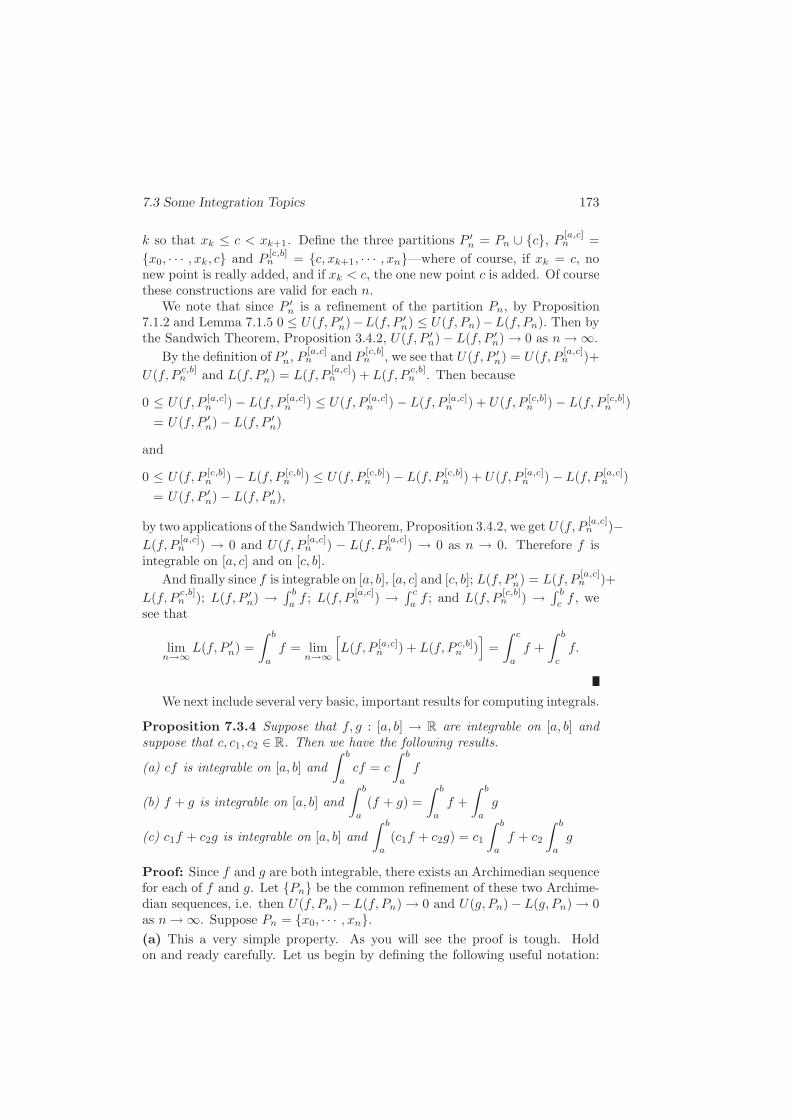
7.3 Some Integration Topics 173
k so that xk ≤ c < xk+1. Define the three partitions P ′n = Pn ∪ {c}, P [a,c]
n =
{x0, · · · , xk, c} and P[c,b]n = {c, xk+1, · · · , xn}—where of course, if xk = c, no
new point is really added, and if xk < c, the one new point c is added. Of coursethese constructions are valid for each n.
We note that since P ′n is a refinement of the partition Pn, by Proposition
7.1.2 and Lemma 7.1.5 0 ≤ U(f, P ′n)−L(f, P ′
n) ≤ U(f, Pn)−L(f, Pn). Then bythe Sandwich Theorem, Proposition 3.4.2, U(f, P ′
n) − L(f, P ′n) → 0 as n→ ∞.
By the definition of P ′n, P
[a,c]n and P
[c,b]n , we see that U(f, P ′
n) = U(f, P[a,c]n )+
U(f, Pc,b]n and L(f, P ′
n) = L(f, P[a,c]n ) + L(f, P
c,b]n . Then because
0 ≤ U(f, P [a,c]n ) − L(f, P [a,c]
n ) ≤ U(f, P [a,c]n ) − L(f, P [a,c]
n ) + U(f, P [c,b]n ) − L(f, P [c,b]
n )
= U(f, P ′n) − L(f, P ′
n)
and
0 ≤ U(f, P [c,b]n ) − L(f, P [c,b]
n ) ≤ U(f, P [c,b]n ) − L(f, P [c,b]
n ) + U(f, P [a,c]n ) − L(f, P [a,c]
n )
= U(f, P ′n) − L(f, P ′
n),
by two applications of the Sandwich Theorem, Proposition 3.4.2, we get U(f, P[a,c]n )−
L(f, P[a,c]n ) → 0 and U(f, P
[a,c]n ) − L(f, P
[a,c]n ) → 0 as n → 0. Therefore f is
integrable on [a, c] and on [c, b].
And finally since f is integrable on [a, b], [a, c] and [c, b]; L(f, P ′n) = L(f, P
[a,c]n )+
L(f, Pc,b]n ); L(f, P ′
n) →∫ b
af ; L(f, P
[a,c]n ) →
∫ c
af ; and L(f, P
[c,b]n ) →
∫ b
cf , we
see that
limn→∞
L(f, P ′n) =
∫ b
a
f = limn→∞
[
L(f, P [a,c]n ) + L(f, P c,b]n )
]
=
∫ c
a
f +
∫ b
c
f.
We next include several very basic, important results for computing integrals.
Proposition 7.3.4 Suppose that f, g : [a, b] → R are integrable on [a, b] andsuppose that c, c1, c2 ∈ R. Then we have the following results.
(a) cf is integrable on [a, b] and
∫ b
a
cf = c
∫ b
a
f
(b) f + g is integrable on [a, b] and
∫ b
a
(f + g) =
∫ b
a
f +
∫ b
a
g
(c) c1f + c2g is integrable on [a, b] and
∫ b
a
(c1f + c2g) = c1
∫ b
a
f + c2
∫ b
a
g
Proof: Since f and g are both integrable, there exists an Archimedian sequencefor each of f and g. Let {Pn} be the common refinement of these two Archime-dian sequences, i.e. then U(f, Pn) − L(f, Pn) → 0 and U(g, Pn) − L(g, Pn) → 0as n→ ∞. Suppose Pn = {x0, · · · , xn}.(a) This a very simple property. As you will see the proof is tough. Holdon and ready carefully. Let us begin by defining the following useful notation:
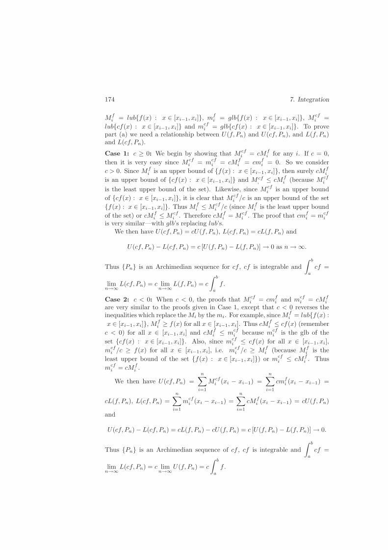
174 7. Integration
Mfi = lub{f(x) : x ∈ [xi−1, xi]}, mf
i = glb{f(x) : x ∈ [xi−1, xi]}, M cfi =
lub{cf(x) : x ∈ [xi−1, xi]} and mcfi = glb{cf(x) : x ∈ [xi−1, xi]}. To prove
part (a) we need a relationship between U(f, Pn) and U(cf, Pn), and L(f, Pn)and L(cf, Pn).
Case 1: c ≥ 0: We begin by showing that M cfi = cMf
i for any i. If c = 0,
then it is very easy since M cfi = mcf
i = cMfi = cmf
i = 0. So we consider
c > 0. Since Mfi is an upper bound of {f(x) : x ∈ [xi−1, xi]}, then surely cMf
i
is an upper bound of {cf(x) : x ∈ [xi−1, xi]} and M cf, ≤ cMf
i (because M cfi
is the least upper bound of the set). Likewise, since M cfi is an upper bound
of {cf(x) : x ∈ [xi−1, xi]}, it is clear that M cfi /c is an upper bound of the set
{f(x) : x ∈ [xi−1, xi]}. Thus Mfi ≤M cf
i /c (since Mfi is the least upper bound
of the set) or cMfi ≤M cf
i . Therefore cMfi = M cf
i . The proof that cmfi = mcf
i
is very similar—with glb’s replacing lub’s.
We then have U(cf, Pn) = cU(f, Pn), L(cf, Pn) = cL(f, Pn) and
U(cf, Pn) − L(cf, Pn) = c [U(f, Pn) − L(f, Pn)] → 0 as n→ ∞.
Thus {Pn} is an Archimedian sequence for cf , cf is integrable and
∫ b
a
cf =
limn→∞
L(cf, Pn) = c limn→∞
L(f, Pn) = c
∫ b
a
f .
Case 2: c < 0: When c < 0, the proofs that M cfi = cmf
i and mcfi = cMf
i
are very similar to the proofs given in Case 1, except that c < 0 reverses theinequalities which replace theMi by themi. For example, sinceMf
i = lub{f(x) :
x ∈ [xi−1, xi]}, Mfi ≥ f(x) for all x ∈ [xi−1, xi]. Thus cMf
i ≤ cf(x) (remember
c < 0) for all x ∈ [xi−1, xi] and cMfi ≤ mcf
i because mcfi is the glb of the
set {cf(x) : x ∈ [xi−1, xi]}. Also, since mcfi ≤ cf(x) for all x ∈ [xi−1, xi],
mcfi /c ≥ f(x) for all x ∈ [xi−1, xi], i.e. mcf
i /c ≥ Mfi (because Mf
i is the
least upper bound of the set {f(x) : x ∈ [xi−1, xi]}) or mcfi ≤ cMf
i . Thus
mcfi = cMf
i .
We then have U(cf, Pn) =
n∑
i=1
M cfi (xi − xi−1) =
n∑
i=1
cmfi (xi − xi−1) =
cL(f, Pn), L(cf, Pn) =
n∑
i=1
mcfi (xi − xi−1) =
n∑
i=1
cMfi (xi − xi−1) = cU(f, Pn)
and
U(cf, Pn) − L(cf, Pn) = cL(f, Pn) − cU(f, Pn) = c [U(f, Pn) − L(f, Pn)] → 0.
Thus {Pn} is an Archimedian sequence of cf , cf is integrable and
∫ b
a
cf =
limn→∞
L(cf, Pn) = c limn→∞
U(f, Pn) = c
∫ b
a
f .

7.3 Some Integration Topics 175
(b) Note that for this proof it is important that we made {Pn} to be thecommon refinement of the Archimedian sequences for both f and g. We didn’tneed it for part (a) but we need it here. For this proof we define Mf
i , mfi as
we did in part (a), and Mgi , mg
i , Mf+gi and mf+g
i analogously. The technicalinequalities that we need, L(f, Pn)+L(g, Pn) ≤ L(f+g, Pn) and U(f+g, Pn) ≤U(f, Pn) + U(g, Pn) follow easily from the inequalities mf
i + mgi ≤ mf+g
i and
Mf+gi ≤ Mf
i + Mgi . For example, for x ∈ [xi−1, xi] we see that mf
i + mgi ≤
f(x)+ g(x). Thus mfi +mg
i ≤ mf+gi (because mf+g
i is the greatest lower boundof the set) which is one of the inequalitiies that we wanted to prove. The otherinequality follows in the same manner.
Thus since both U(f, Pn) − L(f, Pn) → 0 and U(g, Pn) − L(g, Pn) → 0, wehave
U(f + g, Pn) − L(f + g, Pn) ≤ U(f, Pn) + U(g, Pn) − [L(f, Pn) + L(g, Pn)]
= [U(f, Pn) − L(f, Pn)] + [U(g, Pn) − L(g, Pn)]
→ 0 as n→ ∞.
Therefore {Pn} is an Archimedian sequence for f+g on [a, b] so f+g is integrable
on [a, b], and limn→∞
L(f + g, Pn) = limn→∞
U(f + g, Pn) =
∫ b
a
(f + g).
Since we have L(f, Pn)+L(g, Pn) ≤ L(f+g, Pn) ≤ U(f+g, Pn) ≤ U(f, Pn)+U(g, Pn), taking the limit of all parts of the inequality as n→ ∞ gives
∫ b
a
f +
∫ b
a
g ≤∫ b
a
(f + g) ≤∫ b
a
(f + g) ≤∫ b
a
f +
∫ b
a
g
(we don’t really need the extra∫ b
a (f + g) in the inequality). Thus by the
Sandwich Theorem, Proposition 3.4.2,∫ b
a(f + g) =
∫ b
af +
∫ b
ag.
(c) Part (c) follows from parts (a) and (b).
The above proof was not necessarily difficult but very technical. However,we must realize that it is the proof of an important theorem.
HW 7.3.1 (True or False and why) (a) If f : [a, b] → R is integrable on [a, b],then |f | is integrable on [a, b].(b) Suppose f : [a, b] → R. If |f | is integrable on [a, b], then f is integrable on[a, b].(c) If f, g :→ R are not integrable on [0, 1], then f + g is not integrable on [0, 1].(d) If f : [a, b] → R is not integrable on [0, 1], then cf is not integrable on [0, 1]for c ∈ R.(e) If f, g : [0, 1] → R is such that f is continuous on [0, 1] and g is strictlyincreasing on [0, 1], then f + 2g is integrable on [0, 1].
HW 7.3.2 Define f : [0, 2] → R by f(x) =
{
x if x ∈ [0, 1]
3 if x ∈ (1, 2].

176 7. Integration
(a) Find an Archimedian sequence of partitions that shows that f is integrable
on [0, 2]. Find
∫ 2
0
f .
(b) Use the theorems of this section to prove that f is integrable on [0, 2].(c) Prove that f is integrable on [1, 2].
HW 7.3.3 Suppose f, g : [a, b] → R are such that f is continuous on [a, b]and g(x) = f(x) on [a, b] except for a finite number of points. Show that g is
integrable on [a, b] and
∫ b
a
g =
∫ b
a
f .
HW 7.3.4 Consider the function f : [−2, 2] → R defined by
f(x) =
−1 if x ∈ [−2, 1]
x if x ∈ (−1, 1)
1 if x ∈ [1, 2].
Prove that f is integrable on [−2, 2].
7.4 More Topics in Integration
There are many basic, important properties of integration—too many to fit intoone section. Thus this section is actually a continuation of the last section. Thenext proposition that we include at first seems very general and probably notfamiliar. The proof is tough so pay attention. As you will see the propositionwill provide for us some very useful corollaries.
Proposition 7.4.1 Suppose f : [a, b] → R is integrable on [a, b] and φ : [c, d] →R is continuous on [c, d] where f([a, b]) ⊂ [c, d]. Then the function φ◦f : [a, b] →R is integrable on [a, b].
Proof: We will work to find a partition of [a, b] that allows us to apply Rie-mann’s Theorem, Theorem 7.2.6. Let ǫ > 0 be given, let K = lub{|φ(y)| :y ∈ [c, d]} and set ǫ1 = ǫ/(b− a+ 2K) (we’ll see why this is the correct choice
of ǫ1 later). Since φ is continuous on [c, d], φ is uniformly continuous on [c, d].So given ǫ1 > 0 there exists δ such that y1, y2 ∈ [c, d] and |y1 − y2| < δ impliesthat |φ(y1) − φ(y2)| < ǫ1. Choose δ < ǫ1—we can always make our δ smaller.
Since f is integrable on [a, b], by the Riemann Theorem, Theorem 7.2.6, thereexists a partition P such that U(f, P )−L(f, P ) < δ2. (Theorem 7.2.6 said thatwe could find such a partition P for any ǫ > 0—we’re using δ2 in place of the ǫin the theorem.) Suppose P is given by P = {x0, · · · , xn}. The partition P isthe partition we want to use in our application of Theorem 7.2.6 to show thatφ ◦ f is integrable on [a, b], i.e. we must show that U(φ ◦ f, P )−L(φ ◦ f, P ) < ǫ.
We know that
U(f, P ) − L(f, P ) =
n∑
i=1
(Mfi −mf
i )(xi − xi−1) < δ2 (7.4.1)

7.4 More Integration Topics 177
where we will use the notation used in the last theorem: for any F MFi =
lub{F (x) : x ∈ [xi−1, xi]} and mFi = glb{F (x) : x ∈ [xi−1, xi]}.
Since U(f, P )−L(f, P ) must be ”small”, and sinceMfi −mf
i and xi−xi−1 are
both greater than or equal to zero, then (Mfi −mf
i )(xi−xi−1) must be ”small”.
There are two ways the terms (Mfi −mf
i )(xi − xi−1) are made ”small”—either
Mfi −mf
i can be ”small” or xi − xi−1 is ”small”.
Let S1 be the set of indices for which Mfi −mf
i is ”small”, i.e. S1 = {i :
1 ≤ i ≤ n and Mfi −mf
i < δ}. Let S2 = {i : 1 ≤ i ≤ n and Mfi −mf
i ≥ δ}.Note that we have now partially defined what we mean by ”small” and thoughwe have defined the set S2 to be the set of indices on which Mf
i − mfi is not
”small”, it is for these partition intervals that we had better have xi − xi−1 besmall—because we have decided that Mf
i −mfi is not.
We note that
U (φ ◦ f, P ) − L(φ ◦ f, P ) =
n∑
i=1
(Mφ◦fi −mφ◦f
i )(xi − xi−1)
=∑
i∈S1
(Mφ◦fi −mφ◦f
i )(xi − xi−1) +∑
i∈S2
(Mφ◦fi −mφ◦f
i )(xi − xi−1).(7.4.2)
We will handle the two sums separately.
For i ∈ S1: We note that for i ∈ S1 we have Mfi −mf
i < δ. We are interested
in Mφ◦fi −mφ◦f
i . To aid us we prove the following two claims.
Claim 1: Mfi −mf
i = lub{f(x)− f(y) : x, y ∈ [xi−1, xi]}Claim 2: Mφ◦f
i −mφ◦fi = lub{φ(f(x)) − φ(f(y)) : x, y ∈ [xi−1, xi]}
Proof of Claim 2: Recall that Mφ◦fi = lub{φ ◦ f(x) : x ∈ [xi−1, xi]} and
mφ◦fi = glb{φ ◦ f(y) : y ∈ [xi−1, xi]}. By Proposition 1.5.3-(a) for every ǫ3 >
0 there exists φ ◦ f(x∗) ∈ {φ ◦ f(x) : x ∈ [xi−1, xi]} such that Mφ◦fi − φ ◦
f(x∗) < ǫ3/2. Also by Proposition 3.4.2-(b) there exists φ ◦ f(y∗) ∈ {φ ◦ f(y) :
y ∈ [xi−1, xi]} such that φ ◦ f(y∗) − mφ◦fi < ǫ3/2. Then Mφ◦f
i − mφ◦fi −
[φ(f(x∗)) − φ(f(y∗))] < ǫ, i.e. for ǫ3 > 0 there exists
φ ◦ f(x∗) − φ ◦ f(y∗) ∈ {φ(f(x)) − φ(f(y)) : x, y ∈ [xi−1, xi]}
so that Mφ◦fi −mφ◦f
i − [φ(f(x∗)) − φ(f(y∗))] < ǫ3. Thus again by Proposition
3.4.2-(a) Mφ◦fi −mφ◦f
i = lub{φ(f(x)) − φ(f(y)) : x, y ∈ [xi−1, xi]}.The proof of Claim 1 is essentially the same—a bit easier.
By Claim 1 and the fact thatMfi −mf
i < δ we see that for any x, y ∈ [xi−1, xi]we have |f(x) − f(y)| < δ. Then by the uniform continuity of φ, we have for
any x, y ∈ [xi−1, xi] φ(f(x)) − φ(f(y))| < ǫ1. Therefore Mφ◦fi −mφ◦f
i ≤ ǫ1.Therefore we have∑
i∈S1
(Mφ◦fi −mφ◦f
i )(xi − xi−1) ≤ ǫ1∑
i∈S1
(xi − xi−1) ≤ ǫ1(b − a). (7.4.3)

178 7. Integration
For i ∈ S2: We note that for i ∈ S2 we have Mfi − mf
i ≥ δ. Note that
Mφ◦fi = lub{φ ◦ f(x) : x ∈ [xi−1, xi]} ≤ K (x ∈ [xi−1, xi] implies φ(f(x)) ≤
|φ(f(x))| ≤ K) and mφ◦fi = glb{φ ◦ f(x) : x ∈ [xi−1, xi]} ≥ −K (x ∈ [xi−1, xi]
implies φ(f(x)) ≥ −|φ(f(x))| ≥ −K). Then Mφ◦fi −mφ◦f
i ≥ 2K.
If for each i ∈ S2 we multiply both sides of the inequality Mfi −mf
i ≥ δ by
(xi−xi−1) (all positive) and sum over S2, we get∑
i∈S2(Mf
i −mfi )(xi−xi−1) ≥
δ∑
i∈S2(xi − xi−1) or
δ∑
i∈S2
(xi − xi−1) ≤∑
i∈S2
(Mfi −mf
i )(xi − xi−1) ≤n∑
i=1
(Mfi −mf
i )(xi − xi−1) < δ2
(by (7.4.1)) or∑
i∈S2(xi − xi−1) < δ. Thus
U(φ ◦ f, P ) − L(φ ◦ f, P ) =∑
i∈S1
(Mφ◦fi −mφ◦f
i )(xi − xi−1)
+∑
i∈S2
(Mφ◦fi −mφ◦f
i )(xi − xi−1) ≤ ǫ1(b− a) + 2K∑
i∈S2
(xi − xi−1)
< ǫ1(b − a) + 2Kδ < ǫ1(b− a+ 2K) = ǫ.
Therefore by Theorem 7.2.6 the function φ ◦ f is integrable on [a, b].
That too was a very technical proof. As we said earlier Proposition 7.4.1 isuseful for its corollaries. We begin with the following.
Corollary 7.4.2 Suppose f, g : [a, b] → R are integrable on [a, b]. Then(a) f2 is integrable on [a, b], and(b) fn is integrable on [a, b] for any n ∈ N.(c) |f | is integrable on [a, b].(d) fg is integrable on [a, b].
Proof: The proof of part (a) consists of letting φ(y) = y2—which is surelycontinuous anywhere—and applying Proposition 7.4.1. The proof of part (b) isa reasonably nice induction proof using part (a). To obtain part (c) we againuse Proposition 7.4.1, this time with φ(y) = |y|. And part (d) follows by notingthat fg = 1
4
{
(f + g)2 − (f − g)2}
and using Proposition 7.3.4 along with part(a) of this proposition.
We should realize that we can let φ be any continuous function on [c, d]—which will give us a lot of different integrable composite functions. For example,if we let φ(x) = cx we see that the function cf is integrable if f is integrable—part (a) Proposition 7.3.4. We next prove two reasonably easy propositions thatwill give us a lot of interesting, integrable functions.
Proposition 7.4.3 (a) Suppose that f : [a, b] → R is integrable on [a, c] and
[c, b] for c ∈ (a, b). Then f is integrable on [a, b] and
∫ b
a
f =
∫ c
a
f +
∫ b
c
f .

7.4 More Integration Topics 179
(b) Suppose that f : [c0, ck+1] → R, c1, · · · , ck satisfy c0 < c1 < · · · ck < ck+1
and f is integrable on [cj−1, cj ] for j = 1, · · ·k + 1. Then f is integrable on
[c0, ck+1] and
∫ ck+1
c0
f =k+1∑
j=1
∫ cj
cj−1
f .
Proof: (a) Since f is integrable on [a, c] and [c, b], by Theorem 7.2.6 for anyǫ > 0 there exists a partition P1 of [a, c] and a partition P2 of [c, b] such thatU(f, P1) − L(f, P1) < ǫ/2 and U(f, P2) − L(f, P2) < ǫ/2. Let P by the parti-tion P = P1 ∪ P2. Clearly P is a partition of [a, b] and U(f, P ) − L(f, P ) =[U(f, P1) − L(f, P1)] + [U(f, P2) − L(f, P2)] < ǫ. Therefore by Theorem 7.2.6the function f is integrable on [a, b]. We can then apply Proposition 7.3.3 to
see that
∫ b
a
f =
∫ c
a
f +
∫ b
c
f .
(b) Part (b) follows from part (a) using mathematical induction.
Proposition 7.4.4 Suppose f : [a, b] → R is bounded on [a, b] and continuouson (a, b). Then f is integrable on [a, b].
Proof: Since f is bounded on [a, b], there exists some K such that |f(x)| ≤ Kfor x ∈ [a, b]. Let x0 = a, x1 = a+(b−a)/n (for some n, yet to be determined),xn−1 = b − (b − a)/n and xn = b. Note that lub{f(x) : x ∈ [x0, x1]} ≤ K(for x ∈ [x0, x1], f(x) ≤ |f(x)| ≤ K), glb{f(x) : x ∈ [x0, x1]} ≥ −K (forx ∈ [x0, x1], f(x) ≥ −|f(x)| ≥ −K), lub{f(x) : x ∈ [xn−1, xn]} ≤ K, andglb{f(x) : x ∈ [xn−1, xn]} ≥ −K. Thus M1 −m1 ≤ 2K and Mn −mn ≤ 2K.
Now suppose we are given ǫ > 0. Choose n above so that 4K(b−a)/n < ǫ/2.Since f is continuous on (a, b), we know that f is continuous on [x1, xn−1]. Thenby Riemann’s Theorem, Theorem 7.2.6, we know that there exists a partitionP ∗ of [x1, xn−1] such that U(f, P ∗) − L(f, P ∗) < ǫ/2. Write the partitionP ∗ as P ∗ = {x1, x2, · · · , xn−1}. Let P = {x0, x1, · · · , xn−1, xn}, i.e. P =P ∗ ∪ {x0, xn}. Then clearly P is a partition of [a, b] and
U(f, P ) − L(f, P ) = (M1 −m1)(x1 − a) + U(f, P ∗) − L(f, P ∗) + (Mn −mn)(b− xn−1)
< 2K(b− a)/n+ ǫ/2 + 2K(b− a)/n < ǫ.
Then using Theorem 7.2.6 again we get that f is integrable on [a, b].
It might not be clear the range of integrable functions this result produces.If a < c1 < · · · < ck < b, and f is continuous on (a, c1), (ck, b) and (cj−1, cj) forj = 2, · · · , k, then we say that f is piecewise continuous on [a, b]. If we assumethat f is defined at a, c1,· · · ,ck,b (which forces f to be bounded on [a, b]), thenby Propositions 7.4.3 and 7.4.4 we see that f is integrable on [a, b] and
∫ b
a
f =
∫ c1
a
f +
k∑
j=2
∫ cj
cj−1
f +
∫ b
ck
.
Also if we have the same setting a < c1 < · · · < ck < b and S is defined to be con-stant on each open interval (a, c1), (ck, b) and (cj−1, cj), j = 2, · · · , k, then S is

180 7. Integration
said to be a step function. If, in addition S is defined at the points a, c1,· · · ,ck,b,then S is piecewise continuous on [a, b] and is integrable on [a, b]. Thus we havea lot of integrable functions, a bit more interesting than just continuous func-
tions. In fact, we note that the nasty function f(x) =
{
sin(1/x) if x 6= 0
0 if x = 0is
intregrable on [0, 1]. Note also that f is integrable on [−1, 1].We next proof a intuitive result that as we will see later is a useful tool.
Proposition 7.4.5 Suppose that f, g : [a, b] → R are integrable on [a, b] and
satisfy f(x) ≤ g(x) for all ∈ [a, b]. Then∫ b
a f ≤∫ b
a g.
Proof: Since f and g are integrable, they will both have Archimedian sequenceson [a, b]. Let {Pn} be the common refinement of both sequences, i.e. {Pn} will
satisfy U(f, Pn) →∫ b
a
f and U(g, Pn) →∫ b
a
g as n → ∞. Since f(x) ≤ g(x)
on [a, b], f(x) ≤ g(x) on any of the partition intervals [xi−1, xi] and we get
Mfi ≤Mg
i (using notation that we defined in the proof of part (b) of Proposition
7.3.4) and U(f, Pn) ≤ U(g, Pn). If we then let n→ ∞, we get∫ b
a f ≤∫ b
a g.
We next combine Propositions 7.3.4 and 7.4.5 to obtain the following impor-tant result.
Proposition 7.4.6 Suppose that f : [a, b] → R are integrable on [a, b].
(a) Then
∣
∣
∣
∣
∣
∫ b
a
f
∣
∣
∣
∣
∣
≤∫ b
a
|f |.
(b) If |f(x)| ≤M for all x ∈ [a, b], then
∣
∣
∣
∣
∣
∫ b
a
f
∣
∣
∣
∣
∣
≤M(b− a).
Proof: (a) We note that by the definition of absolute value we have −|f(x)| ≤f(x) ≤ |f(x)|. By Corollary 7.4.2-(c) we know that f integrable implies that |f |
is integrable. Then by Proposition 7.4.5 we have
∫ b
a
(−|f |) ≤∫ b
a
f ≤∫ b
a
|f |.
Applying Proposition 7.3.4 gives −∫ b
a
|f |) ≤∫ b
a
f ≤∫ b
a
|f | which gives us∣
∣
∣
∣
∣
∫ b
a
f
∣
∣
∣
∣
∣
≤∫ b
a
|f |.
(b) Before we start let us emphasize that |f(x)| ≤M is not really an hypothesis.Because f is already assumed to be integrable, we know f must be bounded.We’re now just saying that it’s bounded by M .
If we apply part (a) of this proposition and Proposition 7.4.5 we get
∣
∣
∣
∣
∣
∫ b
a
f
∣
∣
∣
∣
∣
≤∫ b
a
|f | ≤∫ b
a
M = (b− a)M which is what we were to prove.
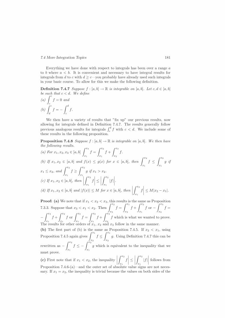
7.4 More Integration Topics 181
Everything we have done with respect to integrals has been over a range ato b where a < b. It is convenient and necessary to have integral results forintegrals from d to c with d ≥ c—you probably have already used such integralsin your basic course. To allow for this we make the following definition.
Definition 7.4.7 Suppose f : [a, b] → R is integrable on [a, b]. Let c, d ∈ [a, b]be such that c < d. We define
(a)
∫ c
c
f = 0 and
(b)
∫ c
d
f = −∫ d
c
f .
We then have a variety of results that ”fix up” our previous results, nowallowing for integrals defined in Definition 7.4.7. The results generally follow
previous analogous results for integrals∫ d
cf with c < d. We include some of
these results in the following proposition.
Proposition 7.4.8 Suppose f : [a, b] → R is integrable on [a, b]. We then havethe following results.
(a) For x1, x2, x3 ∈ [a, b]
∫ x3
x1
f =
∫ x2
x1
f +
∫ x3
x2
f .
(b) If x1, x2 ∈ [a, b] and f(x) ≤ g(x) for x ∈ [a, b], then
∫ x2
x1
f ≤∫ x2
x1
g if
x1 ≤ x2, and
∫ x2
x1
f ≥∫ x2
x1
g if x1 > x2.
(c) If x1, x2 ∈ [a, b], then
∣
∣
∣
∣
∫ x2
x1
f
∣
∣
∣
∣
≤∣
∣
∣
∣
∫ x2
x1
|f |∣
∣
∣
∣
.
(d) If x1, x2 ∈ [a, b] and |f(x)| ≤M for x ∈ [a, b], then
∣
∣
∣
∣
∫ x2
x1
f
∣
∣
∣
∣
≤M |x2 − x1|.
Proof: (a) We note that if x1 < x2 < x3, this results is the same as Proposition
7.3.3. Suppose that x3 < x1 < x2. Then
∫ x2
x3
f =
∫ x1
x3
f +
∫ x2
x1
f or −∫ x3
x2
f =
−∫ x3
x1
f +
∫ x2
x1
f or
∫ x3
x1
f =
∫ x2
x1
f +
∫ x3
x2
f which is what we wanted to prove.
The results for other orders of x1, x2 and x3 follow in the same manner.
(b) The first part of (b) is the same as Proposition 7.4.5. If x2 < x1, using
Proposition 7.4.5 again gives
∫ x1
x2
f ≤∫ x1
x2
g. Using Definition 7.4.7 this can be
rewritten as −∫ x2
x1
f ≤ −∫ x2
x1
g which is equivalent to the inequality that we
must prove.
(c) First note that if x1 < x2, the inequality
∣
∣
∣
∣
∫ x2
x1
f
∣
∣
∣
∣
≤∣
∣
∣
∣
∫ x2
x1
|f |∣
∣
∣
∣
follows from
Proposition 7.4.6-(a)—and the outer set of absolute value signs are not neces-sary. If x1 = x2, the inequality is trivial because the values on both sides of the

182 7. Integration
inequality are zero. And finally, if x1 > x2, then
∣
∣
∣
∣
∫ x2
x1
f
∣
∣
∣
∣
=
∣
∣
∣
∣
−∫ x1
x2
f
∣
∣
∣
∣
=
∣
∣
∣
∣
∫ x1
x2
f
∣
∣
∣
∣
≤∫ x1
x2
|f |
by Proposition 7.4.6-(a). Then since
∫ x1
x2
|f | = −∫ x2
x1
|f | =
∣
∣
∣
∣
∫ x2
x1
|f |∣
∣
∣
∣
, we have
the desired result.
(d) If x1 < x2, this result follows from Proposition 7.4.5-(b). If x1 = x2, bothsides of the inequality are zero—so the result is true. If x1 > x2, we apply
Proposition 7.4.3-(b) to get
∣
∣
∣
∣
∫ x1
x2
f
∣
∣
∣
∣
≤M(x1 − x2). Then
∣
∣
∣
∣
∫ x2
x1
f
∣
∣
∣
∣
=
∣
∣
∣
∣
−∫ x1
x2
f
∣
∣
∣
∣
=
∣
∣
∣
∣
∫ x1
x2
f
∣
∣
∣
∣
≤M(x1 − x2) = M |x2 − x1|.
There may be some other integration results that must be adjusted to allowfor arbitrary limits and from this time on we will assume that you are able tocomplete them.
HW 7.4.1 labelhw7.4.1 (True or False and why) (a) Suppose f : [a, b] → R isintegrable on [a, b]. Then the function g defined by g(x) = sin f(x), x ∈ [a, b],is integrable on [a, b].(b) Suppose f : [a, b] → R is integrable on [a, b], and x1, x2 ∈ [a, b]. Then∣
∣
∣
∣
∫ x2
x1
f
∣
∣
∣
∣
≤∫ x2
x1
|f |.
(c) Suppose f : [a, b] → R is such that f(x) > 0 for x ∈ [a, b]. Then
∫ b
a
f > 0.
(d) Suppose f : [a, b] → R is integrable on [a, b] and such that f(x) > 0 for
x ∈ [a, b]. Then
∫ b
a
f > 0.
(e) Suppose f : [a, b] → R is integrable on [a, b] and there exists a c > 0 suchthat f(x) ≥ c for all x ∈ [a, b]. Then 1/f is integrable on [a, b].
HW 7.4.2 Recall that we earlier defined functions f1(x) =
{
sin(1/x) if x 6= 0
0 if x = 0,
f2(x) =
{
x sin(1/x) if x 6= 0
0 if x = 0and f3(x) =
{
x2 sin(1/x) if x 6= 0
0 if x = 0.
Which of the functions f1, f2 and f3 are integrable on [−1, 1]—prove it.
HW 7.4.3 Suppose f : [0, 1] → R is continuous on [0, 1] and that
∫ 1
0
f > 0.
Prove that there exists an interval (α, β) ⊂ [0, 1] such that f(x) > 0 for x ∈(α, β).
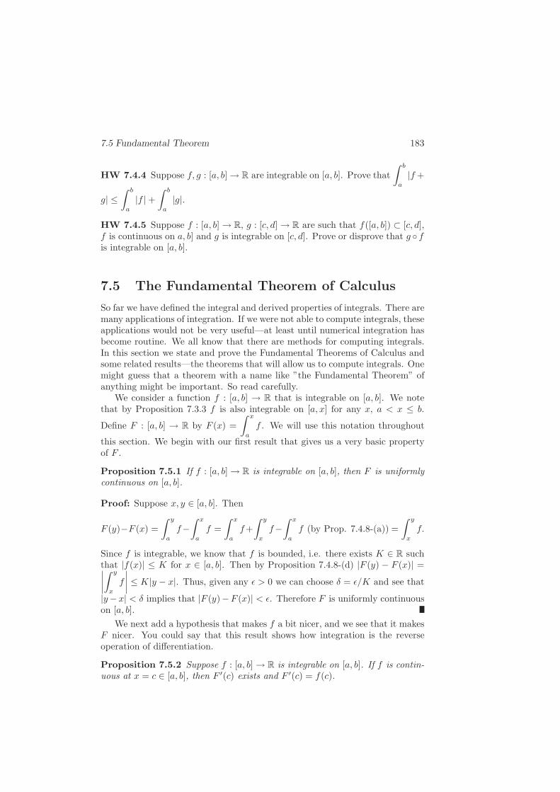
7.5 Fundamental Theorem 183
HW 7.4.4 Suppose f, g : [a, b] → R are integrable on [a, b]. Prove that
∫ b
a
|f+
g| ≤∫ b
a
|f | +∫ b
a
|g|.
HW 7.4.5 Suppose f : [a, b] → R, g : [c, d] → R are such that f([a, b]) ⊂ [c, d],f is continuous on a, b] and g is integrable on [c, d]. Prove or disprove that g ◦ fis integrable on [a, b].
7.5 The Fundamental Theorem of Calculus
So far we have defined the integral and derived properties of integrals. There aremany applications of integration. If we were not able to compute integrals, theseapplications would not be very useful—at least until numerical integration hasbecome routine. We all know that there are methods for computing integrals.In this section we state and prove the Fundamental Theorems of Calculus andsome related results—the theorems that will allow us to compute integrals. Onemight guess that a theorem with a name like ”the Fundamental Theorem” ofanything might be important. So read carefully.
We consider a function f : [a, b] → R that is integrable on [a, b]. We notethat by Proposition 7.3.3 f is also integrable on [a, x] for any x, a < x ≤ b.
Define F : [a, b] → R by F (x) =
∫ x
a
f . We will use this notation throughout
this section. We begin with our first result that gives us a very basic propertyof F .
Proposition 7.5.1 If f : [a, b] → R is integrable on [a, b], then F is uniformlycontinuous on [a, b].
Proof: Suppose x, y ∈ [a, b]. Then
F (y)−F (x) =
∫ y
a
f−∫ x
a
f =
∫ x
a
f+
∫ y
x
f−∫ x
a
f (by Prop. 7.4.8-(a)) =
∫ y
x
f.
Since f is integrable, we know that f is bounded, i.e. there exists K ∈ R suchthat |f(x)| ≤ K for x ∈ [a, b]. Then by Proposition 7.4.8-(d) |F (y) − F (x)| =∣
∣
∣
∣
∫ y
x
f
∣
∣
∣
∣
≤ K|y − x|. Thus, given any ǫ > 0 we can choose δ = ǫ/K and see that
|y− x| < δ implies that |F (y)−F (x)| < ǫ. Therefore F is uniformly continuouson [a, b].
We next add a hypothesis that makes f a bit nicer, and we see that it makesF nicer. You could say that this result shows how integration is the reverseoperation of differentiation.
Proposition 7.5.2 Suppose f : [a, b] → R is integrable on [a, b]. If f is contin-uous at x = c ∈ [a, b], then F ′(c) exists and F ′(c) = f(c).
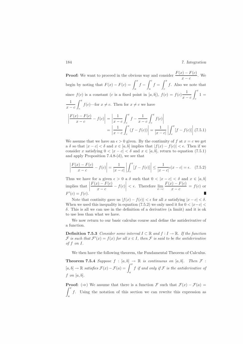
184 7. Integration
Proof: We want to proceed in the obvious way and considerF (x) − F (c)
x− c. We
begin by noting that F (x) − F (c) =
∫ x
a
f −∫ c
a
f =
∫ x
c
f . Also we note that
since f(c) is a constant (c is a fixed point in [a, b]), f(c) = f(c)1
x− c
∫ x
c
1 =
1
x− c
∫ x
c
f(c)—for x 6= c. Then for x 6= c we have
∣
∣
∣
∣
F (x) − F (c)
x− c− f(c)
∣
∣
∣
∣
=
∣
∣
∣
∣
1
x− c
∫ x
c
f − 1
x− c
∫ x
c
f(c)
∣
∣
∣
∣
=
∣
∣
∣
∣
1
x− c
∫ x
c
(f − f(c))
∣
∣
∣
∣
=1
|x− c|
∣
∣
∣
∣
∫ x
c
[f − f(c)]
∣
∣
∣
∣
.(7.5.1)
We assume that we have an ǫ > 0 given. By the continuity of f at x = c we geta δ so that |x − c| < δ and x ∈ [a, b] implies that |f(x) − f(c)| < ǫ. Then if weconsider x satisfying 0 < |x − c| < δ and x ∈ [a, b], return to equation (7.5.1)and apply Proposition 7.4.8-(d), we see that
∣
∣
∣
∣
F (x) − F (c)
x− c− f(c)
∣
∣
∣
∣
=1
|x− c|
∣
∣
∣
∣
∫ x
c
[f − f(c)]
∣
∣
∣
∣
≤ 1
|x− c|ǫ|x− c| = ǫ. (7.5.2)
Thus we have for a given ǫ > 0 a δ such that 0 < |x − c| < δ and x ∈ [a, b]
implies that
∣
∣
∣
∣
F (x) − F (c)
x− c− f(c)
∣
∣
∣
∣
< ǫ. Therefore limx→c
F (x) − F (c)
x− c= f(c) or
F ′(c) = f(c).
Note that continity gave us |f(x) − f(c)| < ǫ for all x satisfying |x− c| < δ.When we used this inequality in equation (7.5.2) we only used it for 0 < |x−c| <δ. This is all we can use in the definition of a derivative (a limiit) and it is okto use less than what we have.
We now return to our basic calculus course and define the antiderivative ofa function.
Definition 7.5.3 Consider some interval I ⊂ R and f : I → R. If the functionF is such that F ′(x) = f(x) for all x ∈ I, then F is said to be the antiderivativeof f on I.
We then have the following theorem, the Fundamental Theorem of Calculus.
Theorem 7.5.4 Suppose f : [a, b] → R is continuous on [a, b]. Then F :
[a, b] → R satisfies F(x)−F(a) =
∫ x
a
f if and only if F is the antiderivative of
f on [a, b].
Proof: (⇒) We assume that there is a function F such that F(x) − F(a) =∫ x
a
f . Using the notation of this section we can rewrite this expression as

7.5 Fundamental Theorem 185
F(x) − F(a) = F (x) and this expression holds for all x ∈ [a, b]. Then since byProposition 7.5.2 F is differentiable on [a, b], we know that F is differentiable on[a, b] (F(a) is a constant). Also by Proposition 7.5.2 and the fact that we knowthat the derivative of a constant is zero, we see that F ′(x) = F ′(x) = f(x).Thus F is the antiderivative of f .
(⇐) If F : [a, b] → R is such that F ′(x) = f(x) for x ∈ [a, b], we know thatF ′(x) = F ′(x). By Corollary 6.3.5 there exists a C ∈ R such that F(x) =F (x) + C. Since F (a) = 0, we evaluate the last expression at x = a to see thatF(a) = F (a) + C = C. Thus we have F(x) = F (x) + F(a) or F(x) − F(a) =F (x) =
∫ x
a f which is what we were to prove.
If we let x = b, we get the following corollary that looks more like the resultwe applied so often in our basic course.
Corollary 7.5.5 Suppose f : [a, b] → R is continuous on [a, b] and F is the
antiderivative of f on [a, b]. Then F(b) −F(a) =
∫ b
a
f .
Thus as we have done so often before, we evaluate
∫ 1
0
(x2 + x+ 1) =
[
x3
3+x2
2+ x
]1
0
=
(
1
3+
1
2+ 1
)
− 0 =11
6= F(1) −F(0)
where F(x) = x3
3 + x2
2 + x.
We next include several very nice results, the first two of which are by-products of our previous results. We begin with integration by parts. Inte-gration by parts is usually presented as a technique for evaluating integrals—integrals that we can not evaluated using easier methods. However, with theadvent of computer and calculator calculus systems, integration by parts is notas necessary as an integration technique as it was in the past. Integration byparts is an important tool in analysis as we shall see in the next chapter. Weproceed with the following result.
Proposition 7.5.6 (Integration by Parts) Suppose f, g : [a, b] → R aredifferentiable on [a, b] and are such that f ′, g′ : [a, b] → R are continuous on[a, b] (f and g are continuously differentiable on [a, b]). Then
∫ b
a
f ′g = [f(b)g(b) − f(a)g(a)] −∫ b
a
fg′.
Proof: The proof of the integration by parts formula is very easy. We all
remember that the product formula for differentiation gives usd
dx(fg) = f ′g +
fg′. We integrate both sides of this equality, use Corollary 7.5.5 and get
∫ b
a
d
dx(fg) = f(b)g(b) − f(a)g(a) =
∫ b
a
f ′g +
∫ b
a
fg′.
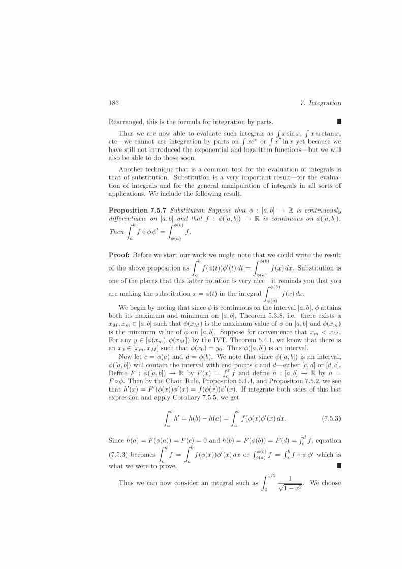
186 7. Integration
Rearranged, this is the formula for integration by parts.
Thus we are now able to evaluate such integrals as∫
x sinx,∫
x arctanx,etc—we cannot use integration by parts on
∫
xex or∫
x7 lnx yet because wehave still not introduced the exponential and logarithm functions—but we willalso be able to do those soon.
Another technique that is a common tool for the evaluation of integrals isthat of substitution. Substitution is a very important result—for the evalua-tion of integrals and for the general manipulation of integrals in all sorts ofapplications. We include the following result.
Proposition 7.5.7 Substitution Suppose that φ : [a, b] → R is continuouslydifferentiable on [a, b] and that f : φ([a, b]) → R is continuous on φ([a, b]).
Then
∫ b
a
f ◦ φφ′ =
∫ φ(b)
φ(a)
f .
Proof: Before we start our work we might note that we could write the result
of the above proposition as
∫ b
a
f(φ(t))φ′(t) dt =
∫ φ(b)
φ(a)
f(x) dx. Substitution is
one of the places that this latter notation is very nice—it reminds you that you
are making the substitution x = φ(t) in the integral
∫ φ(b)
φ(a)
f(x) dx.
We begin by noting that since φ is continuous on the interval [a, b], φ attainsboth its maximum and minimum on [a, b], Theorem 5.3.8, i.e. there exists axM , xm ∈ [a, b] such that φ(xM ) is the maximum value of φ on [a, b] and φ(xm)is the minimum value of φ on [a, b]. Suppose for convenience that xm < xM .For any y ∈ [φ(xm), φ(xM ]) by the IVT, Theorem 5.4.1, we know that there isan x0 ∈ [xm, xM ] such that φ(x0) = y0. Thus φ([a, b]) is an interval.
Now let c = φ(a) and d = φ(b). We note that since φ([a, b]) is an interval,φ([a, b]) will contain the interval with end points c and d—either [c, d] or [d, c].Define F : φ([a, b]) → R by F (x) =
∫ x
c f and define h : [a, b] → R by h =F ◦φ. Then by the Chain Rule, Proposition 6.1.4, and Proposition 7.5.2, we seethat h′(x) = F ′(φ(x))φ′(x) = f(φ(x))φ′(x). If integrate both sides of this lastexpression and apply Corollary 7.5.5, we get
∫ b
a
h′ = h(b) − h(a) =
∫ b
a
f(φ(x)φ′(x) dx. (7.5.3)
Since h(a) = F (φ(a)) = F (c) = 0 and h(b) = F (φ(b)) = F (d) =∫ d
cf , equation
(7.5.3) becomes
∫ d
c
f =
∫ b
a
f(φ(x))φ′(x) dx or∫ φ(b)
φ(a) f =∫ b
a f ◦ φφ′ which is
what we were to prove.
Thus we can now consider an integral such as
∫ 1/2
0
1√1 − x2
. We choose

7.5 Fundamental Theorem 187
φ(θ) = sin θ. Then φ(0) = 0 and φ(π/2) = 1/2. Thus
∫ φ(π/6)
φ(0)
1√1 − x2
=
∫ φ(π/2)
φ(0)
1√
1 − φ(x)φ′(x)
=
∫ π/6
0
cos θ√
1 − sin2 θ=
∫ π/6
0
1 =π
6.
We next include a theorem that may not be familiar to you. We will finduseful in the next chapter and can be used in a variety of interesting ways. Thetheorem is called the Mean Value Theorem for Integrals.
Theorem 7.5.8 (Mean Value Theorem for Integrals) Suppose that f :[a, b] → R is continuous on [a, b], and p : [a, b] → R is integrable on [a, b] andsuch that p(x) ≥ 0 for x ∈ [a, b]. Then there exists c ∈ [a, b]such that
∫ b
a
fp = f(c)
∫ b
a
p. (7.5.4)
Proof: We know from Corollary 7.4.2-(d) that since f and p are integrableon [a, b], fp is integrable on [a, b]. We also know from Theorem 5.3.8 thatf assumes its maximum and minimum on [a, b], i.e there exists m,M ∈ R
such that m ≤ f(x) ≤ M for x ∈ [a, b], and there exists xm, xM ∈ [a, b] suchthat f(xm) = m and f(xM ) = M . Because p(x) ≥ 0 we know also thatmp(x) ≤ f(x)p(x) ≤Mp(x) for all x ∈ [a, b]. Therefore
m
∫ b
a
p ≤∫ b
a
fp ≤M
∫ b
a
p. (7.5.5)
If∫ b
a p = 0, then
∫ b
a
fp = 0 and we can choose any c ∈ [a, b] to satisfy
equation (7.5.4). Otherwise we rewrite inequality (7.5.5) as
f(xm) = m ≤∫ b
afp
∫ b
a p≤M = f(xM ).
Then by the Intermediate Value Theorem, Theorem 5.4.1, (applied on either[xm, xM ] or [xM , xm] depending on whether xm ≤ xM or xM < xm) there exists
c between xm and xM such that f(c) =
∫ b
afp
∫ b
a pwhich is the same as (7.5.4).
HW 7.5.1 (True or False and why) (a) Suppose f : [a, b] → R is continuous on
[a, b]. Thend
dx
[
∫ b
x
f
]
= −f(x).
(b) Suppose f : [a, b] → R is continuous on [a, b]. Thend
dx
[∫ a
x
f
]
= −f(x).

188 7. Integration
(c) Consider f : [−2, 2] → R defined by f(x) =
−2 if x ∈ [−2,−1]
x if x ∈ (−1, 1)
3 if x ∈ [1, 2].
Then the function F (x) =∫ x
−2 f is continuous at points x ∈ [−2,−1)∪ (−1, 1)∪(1, 2] and discontinuous at x = −1 and x = 1.(d) The function F defined in part (c) is differentiable for all x ∈ [−2, 2].(e) Suppose f : [a, b] → R is continuous on [a, b]. Then there exists c ∈ [a, b]
such that
∫ b
a
f = f(c)(b− a).
HW 7.5.2 Consider the functions defined in HW7.5.1-(c). Compute F . PlotF .
HW 7.5.3 Calculate the following three integrals—verifying all steps. (a)∫ 2
−1
x3 (b)
∫ 3
−1
x cosx (c)
∫ 2
1
1√2x− 1
.
HW 7.5.4 Suppose f : [a, b] → R is integrable. Show that there may not be a
c ∈ [a, b] such that
∫ b
a
= f(c)(b− a).
HW 7.5.5 Suppose f, φ, ψ : [a, b] → R are such that f is continuous on [a, b]
and φ and ψ are differentiable on (a, b). Show that for x ∈ (a, b)d
dx
∫ φ(x)
ψ(x)
f =
f(φ(x))φ′(x) − f(ψ(x))ψ′(x).
7.6 The Riemann Integral
The integral studied in the basic calculus course is most often referred to as theRiemann integral. We called the integral that we defined the Darboux integralor just the integral to differentiate it from the integral defined in this section.As we will see in Theorem 7.6.3 the name is not relevant because the integralsare the always equal. It is important to introduce the definition given belowbecause this is the most common definition introduced in the basic calculuscourses. We begin with some definitions.
For a partition of [a, b], P = {x0, x1, · · · , xn−1, xn}, we define the gap of Pto be gap(P ) = max{xi − xi−1 : i = 1, · · · , n}. Thus the gap(P ) is the lengthof the largest partition interval. We then make the following definition.
Definition 7.6.1 Consider the function f : [a, b] → R where f is bounded on[a, b] and let P = {x0, x1, · · · , xn} be a partition of [a, b].
(a) A Riemann sum of f with respect to the partition P is the sum
Sn(f, P ) =
n∑
i=1
f(ξi)(xi − xi−1) (7.6.1)

7.6 Riemann Integral 189
where ξi is any point in [xi−1, xi].
(b) The function f is said to be Riemann integrable on [a, b] if there exists
a real number (R)
∫ b
a
f so that for every ǫ > 0 there exists a δ such that∣
∣
∣
∣
∣
(R)
∫ b
a
f − Sn(f, P )
∣
∣
∣
∣
∣
< ǫ for all partitions P with gap(P ) < δ and all different
choices of Sn(f, P ).
Before we move on let us emphasize some important points here. The Rie-mann sums are very difficult in that for a given partition there are many dif-ferent sums—you get a different value for each choice of ξi ∈ [xi−1, xi] for eachi = 1, · · · , n. That is why we included the statement ”all different choices ofSn(f, P )” in the definition of the Riemann integral—it’s usually not there. The
fact that we must be able to show that
∣
∣
∣
∣
∣
(R)
∫ b
a
f − Sn(f, P )
∣
∣
∣
∣
∣
< ǫ for arbitrary
ξi ∈ [xi−1, xi] (besides all partitions P for which gap(P ) < δ) can make workingwith this definition difficult.
The definition given above is the most common definition used in elementarytextbooks. This is probably because it is the definition that can be given asquickly as possible. In most texts this definition is given before they considerlimits of sequences—let alone limits of partial sums.
We are going to do very little with Definition 7.6.1. As we stated earlier themain result will be Theorem 7.6.3 were we prove that the Riemann integral andthe Darboux integral are the same. Before we do this, we state the followingeasy result.
Proposition 7.6.2 Consider f : [a, b] → R where f is bounded on [a, b]. Iff is Riemann integrable on [a, b], then there exist a sequence of partitions of
[a, b], {Pn} such that Sn(f, Pn) → (R)∫ b
af as n → ∞ for all choices of ξi ∈
[xi−1, x− i], i = 1, · · ·n, i.e. limn→∞
Sn(f, Pn) = (R)
∫ b
a
f for arbitrary ξi.
Proof: We begin by setting ǫn = 1/n, n = 1, · · · and applying Definition7.6.1. For each n we obtain a δn that for any partition of [a, b], P ∗
n , with
gap(P ∗n) < δn satisfies
∣
∣
∣
∣
∣
Sn(f, P∗n) − (R)
∫ b
a
f
∣
∣
∣
∣
∣
< 1/n. For each n choose one
such partition, call it Pn. Then we have a sequence of partitions of [a, b] such
that Sn(f, Pn) → (R)
∫ b
a
f as n→ ∞.
Thus we see that the Riemann integral can be evaluated by a sequence ofthe Riemann sums over a sequence of partitions—much like the result of theArchimedes-Riemann Theorem, Theorem 7.2.4. The real result that we want isthat the Riemann integral defined by Definition 7.6.1 is the same as the Darbouxintegral defined by Definition 7.2.3.
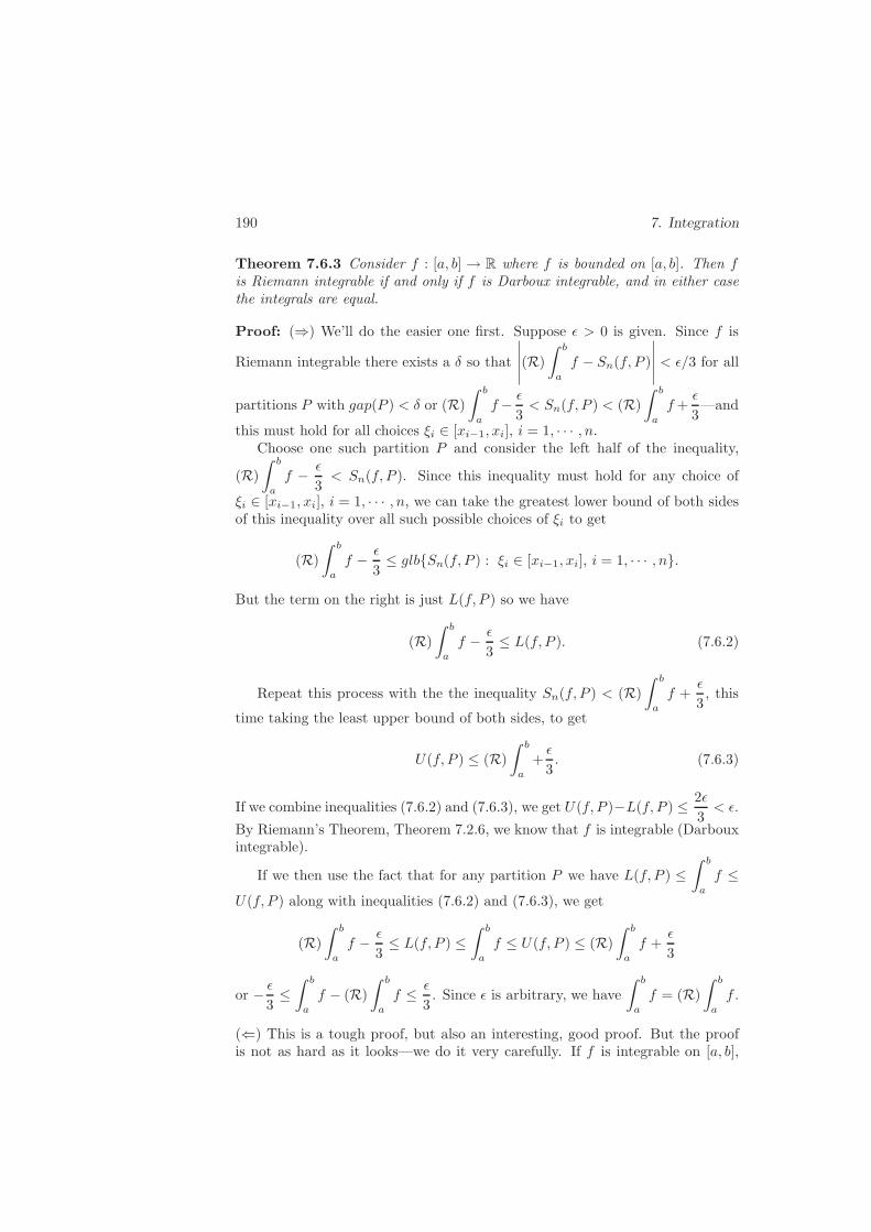
190 7. Integration
Theorem 7.6.3 Consider f : [a, b] → R where f is bounded on [a, b]. Then fis Riemann integrable if and only if f is Darboux integrable, and in either casethe integrals are equal.
Proof: (⇒) We’ll do the easier one first. Suppose ǫ > 0 is given. Since f is
Riemann integrable there exists a δ so that
∣
∣
∣
∣
∣
(R)
∫ b
a
f − Sn(f, P )
∣
∣
∣
∣
∣
< ǫ/3 for all
partitions P with gap(P ) < δ or (R)
∫ b
a
f− ǫ
3< Sn(f, P ) < (R)
∫ b
a
f+ǫ
3—and
this must hold for all choices ξi ∈ [xi−1, xi], i = 1, · · · , n.Choose one such partition P and consider the left half of the inequality,
(R)
∫ b
a
f − ǫ
3< Sn(f, P ). Since this inequality must hold for any choice of
ξi ∈ [xi−1, xi], i = 1, · · · , n, we can take the greatest lower bound of both sidesof this inequality over all such possible choices of ξi to get
(R)
∫ b
a
f − ǫ
3≤ glb{Sn(f, P ) : ξi ∈ [xi−1, xi], i = 1, · · · , n}.
But the term on the right is just L(f, P ) so we have
(R)
∫ b
a
f − ǫ
3≤ L(f, P ). (7.6.2)
Repeat this process with the the inequality Sn(f, P ) < (R)
∫ b
a
f +ǫ
3, this
time taking the least upper bound of both sides, to get
U(f, P ) ≤ (R)
∫ b
a
+ǫ
3. (7.6.3)
If we combine inequalities (7.6.2) and (7.6.3), we get U(f, P )−L(f, P ) ≤ 2ǫ
3< ǫ.
By Riemann’s Theorem, Theorem 7.2.6, we know that f is integrable (Darbouxintegrable).
If we then use the fact that for any partition P we have L(f, P ) ≤∫ b
a
f ≤U(f, P ) along with inequalities (7.6.2) and (7.6.3), we get
(R)
∫ b
a
f − ǫ
3≤ L(f, P ) ≤
∫ b
a
f ≤ U(f, P ) ≤ (R)
∫ b
a
f +ǫ
3
or − ǫ
3≤∫ b
a
f − (R)
∫ b
a
f ≤ ǫ
3. Since ǫ is arbitrary, we have
∫ b
a
f = (R)
∫ b
a
f .
(⇐) This is a tough proof, but also an interesting, good proof. But the proofis not as hard as it looks—we do it very carefully. If f is integrable on [a, b],

7.6 Riemann Integral 191
then for ǫ > 0 by Definitions 7.2.1 and 7.2.3 there exists a partition of [a, b],P ′ = {x0, · · · , xn}, such that
U(f, P ′) −∫ b
a
f = U(f, P ′) −∫ b
a
f <ǫ
4. (7.6.4)
Since f is bounded on [a, b], there existsM such that |f(x)| ≤M for all x ∈ [a, b].Set δ1 = ǫ/16Mn and let P = {y0, y1, · · · , ym} be any partition of [a, b] such
that gap(P ) < δ1. Let P ∗ be the common refinement of P ′ and P , P ∗ = P ′∪P .By Lemma 7.1.5 U(f, P ∗) ≤ U(f, P ′). Then from (7.6.4) we get
U(f, P ∗) −∫ b
a
f <ǫ
4. (7.6.5)
We next want to transfer the information from inequality (7.6.5) to partitionP . To do this we want to compare U(f, P ∗) and U(f, P ), and we will do thisbe looking at 0 ≤ U(f, P ) − U(f, P ∗). Write P ∗ as P ∗ = {z0, z1, · · · , zp}where p will be less than or equal to m + (n − 1)—but we don’t care aboutthis. Define the notation MP∗
i = lub{f(x) : x ∈ [zi−1, zi]}, i = 1, · · · , p, andMPj = lub{f(x) : x ∈ [yj−1, yj ]}, j = 1, · · · ,m. We note the following facts.
• If a partition interval of P , [yj−1, yj ], contains no points of P ′, then thispartition interval is the same as one of the partition intervals of P ∗, MP∗
j =
MPj and the contribution of this interval to U(f, P ) − U(f, P ∗) is zero.
• If a partition interval of P , [yj−1, yj], contains one point of P ′, then thispartition interval is the same as two adjacent partition intervals of P ∗, say[zi−1, zi] and [zi, zi+1] and the contribution of this interval to U(f, P ) −U(f, P ∗) is
MPj (yj − yj−1) − [MP∗
i (zi − zi−1) +MP∗
i+1(zi+1 − zi)]
= MPj [(zi+1 − zi) + (zi − zi−1)] − [MP∗
i (zi − zi−1) +MP∗
i+1(zi+1 − zi)]
= (MPi −MP∗
j )(zi − zi−1) + (MPi+1 −MP∗
j )(zi+1 − zi).
Since either MPj = MP∗
i or MPj = MP∗
i+1, at least one of these twoterms will be zero and the contribution to U(f, P ) − U(f, P ∗) will be(MP
i −MP∗
j )(zi − zi−1) or (MPi+1 −MP∗
j )(zi+1 − zi), and in either casethe contribution will be less than or equal to 2Mδ1 (for example
|(MPi −MP∗
j )(zi−zi−1)| ≤ |(MPi −MP∗
j )|δ1 ≤ (|MPi |+|MP∗
j |)δ1 ≤ 2Mδ1.)
• If a partition interval of P , [yj−1, yj ], contains two points of P ′, then thispartition interval is the same as three adjacent partition intervals of P ∗, weplay the same game—this time with three intervals of P ∗—and find thatthe contribution to U(f, P )−U(f, P ∗) is less than or equal to 2 · 2Mδ1—where the boldface 2 indicates that there will be two terms contributingto this contribution—still only one adds out.
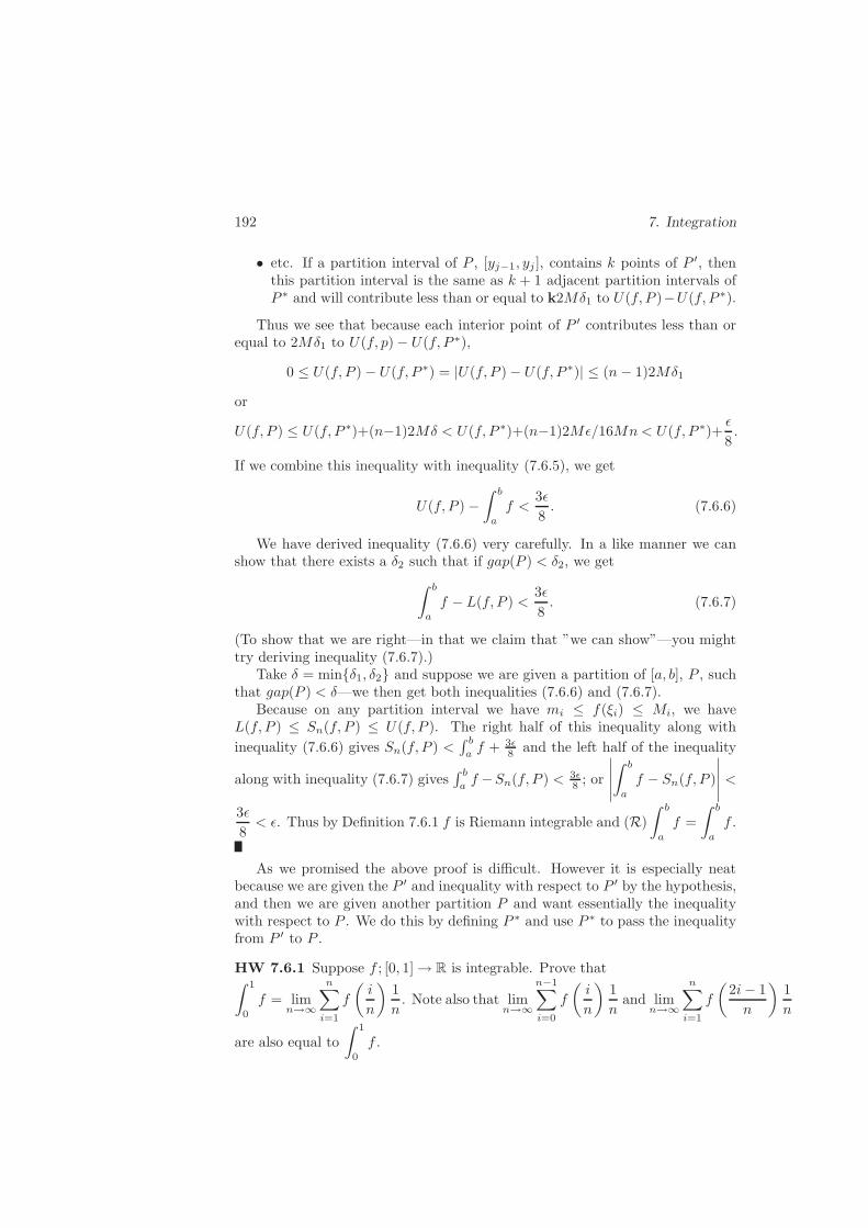
192 7. Integration
• etc. If a partition interval of P , [yj−1, yj ], contains k points of P ′, thenthis partition interval is the same as k + 1 adjacent partition intervals ofP ∗ and will contribute less than or equal to k2Mδ1 to U(f, P )−U(f, P ∗).
Thus we see that because each interior point of P ′ contributes less than orequal to 2Mδ1 to U(f, p) − U(f, P ∗),
0 ≤ U(f, P ) − U(f, P ∗) = |U(f, P ) − U(f, P ∗)| ≤ (n− 1)2Mδ1
or
U(f, P ) ≤ U(f, P ∗)+(n−1)2Mδ < U(f, P ∗)+(n−1)2Mǫ/16Mn< U(f, P ∗)+ǫ
8.
If we combine this inequality with inequality (7.6.5), we get
U(f, P ) −∫ b
a
f <3ǫ
8. (7.6.6)
We have derived inequality (7.6.6) very carefully. In a like manner we canshow that there exists a δ2 such that if gap(P ) < δ2, we get
∫ b
a
f − L(f, P ) <3ǫ
8. (7.6.7)
(To show that we are right—in that we claim that ”we can show”—you mighttry deriving inequality (7.6.7).)
Take δ = min{δ1, δ2} and suppose we are given a partition of [a, b], P , suchthat gap(P ) < δ—we then get both inequalities (7.6.6) and (7.6.7).
Because on any partition interval we have mi ≤ f(ξi) ≤ Mi, we haveL(f, P ) ≤ Sn(f, P ) ≤ U(f, P ). The right half of this inequality along with
inequality (7.6.6) gives Sn(f, P ) <∫ b
af + 3ǫ
8 and the left half of the inequality
along with inequality (7.6.7) gives∫ b
af −Sn(f, P ) < 3ǫ
8 ; or
∣
∣
∣
∣
∣
∫ b
a
f − Sn(f, P )
∣
∣
∣
∣
∣
<
3ǫ
8< ǫ. Thus by Definition 7.6.1 f is Riemann integrable and (R)
∫ b
a
f =
∫ b
a
f .
As we promised the above proof is difficult. However it is especially neatbecause we are given the P ′ and inequality with respect to P ′ by the hypothesis,and then we are given another partition P and want essentially the inequalitywith respect to P . We do this by defining P ∗ and use P ∗ to pass the inequalityfrom P ′ to P .
HW 7.6.1 Suppose f ; [0, 1] → R is integrable. Prove that∫ 1
0
f = limn→∞
n∑
i=1
f
(
i
n
)
1
n. Note also that lim
n→∞
n−1∑
i=0
f
(
i
n
)
1
nand lim
n→∞
n∑
i=1
f
(
2i− 1
n
)
1
n
are also equal to
∫ 1
0
f .

7.7 Logarithms and Exponentials 193
HW 7.6.2 (a) Suppose f : [0, 1] → R and suppose limn→∞
n∑
i=1
f
(
i
n
)
1
nexists.
Show that f is not necessarily integrable on [0, 1].(b) Show also that neither of the other limits of sums considered in HW7.6.1will imply the integrability of f either.
7.7 Logarithm and Exponential Functions
We have been reasonably careful not to use logarithms yet because one of thevery logical ways to define a logarithm is to use the integral as a part of thedefinition (at least we haven’t used them often—surely we haven’t used themfor anything important). We’ve also stayed away from all different kinds ofexponentials where the exponent is anything other than a rational, i.e. we havenot allowed irrational exponents—and we want them and need them. Approxi-mately half of the basic calculus books use this approach to define the logarithmand exponential functions—the books that are not referred to as ”early tran-scendentals”. We make the following definition.
Definition 7.7.1 For x > 0 we define lnx =
∫ x
1
1
tdt which we call the loga-
rithm of x.
We immediately get the following proposition that includes some of the ba-sic results concerning the logarithm function. Since the function f(t) = 1
t iscontinuous for t > 0, we apply Proposition 7.5.2 to obtain the following result.
Proposition 7.7.2 (a) The function ln : (0,∞) → R is continuous on (0,∞).(b) The function ln is differentiable on (0,∞), and d
dx lnx = 1x .
(c) The function ln is strictly increasing.(d) ln 1 = 0.
Proof: We are going to apply Propositions 7.5.1 and 7.5.2. Both of thesepropositions considered a function f defined on a closed interval [a, b]. Forthis result we must consider the function 1/t defined on (0,∞). However, forany x0 ∈ R we can consider [x0/2, 2x0] and apply Propositions 7.5.1 and 7.5.2to see that f(x) = lnx is both continuous and differentiable at t = x0, andd
dxlnx
∣
∣
∣
∣
x=x0
=1
x0. Thus for any x ∈ (0,∞),
d
dxln x =
1
x.
Sinced
dxlnx =
1
x> 0 on (0,∞), the function ln is strictly increasing by
Corollary 6.3.6-(a). (Notice that Corollary 6.3.6-(a) was proved for open in-
tervals. For any x1, x2 ∈ (0,∞) such that x1 < x2,d
dxlnx =
1
x> 0 on
I = (x1/2, x2 + 1). Then by Corollary 6.3.6-(a) ln is strictly increasing on Iso lnx1 < lnx2. Thus the ln function is strictly increasing on (0,∞). Notice

194 7. Integration
also that it would have been easier to just say that ln is strictly increasing byCorollary 6.3.6-(b).)
And by Definition 7.4.7-(a) we see that ln 1 =∫ 1
11t dt.
We next need to show that the logarithm function defined satisfies the basicproperties that we all know logarithm functions are supposed to satisfy.
Proposition 7.7.3 For a, x ∈ (0,∞) and r ∈ Q
(a) ln(ax) = ln a+ lnx(b) ln(a/x) = ln a− lnx(c) lnxr = r lnx
Proof: Notice that the derivative found in part (b) of Proposition 7.7.2 along
with the Chain Rule, Proposition 6.1.4, ddx ln f(x) = f ′(x)
f(x) .
(a) We consider the expression ln(ax) where a ∈ (0,∞) is some constant. Thenddx ln(ax) = a
ax = 1x . Also d
dx (ln a + lnx) = 0 + 1x = 1
x . Since ddx ln(ax) =
ddx(ln a + lnx) = 1
x , by Corollary 6.3.5 we know that ln(ax) = ln a + lnx + Cwhere C is some constant. This last equality must be true for all x ∈ (0,∞).We set x = 1 to see that ln a = ln a + ln 1 + C = ln a + C or C = 0. Thusln(ax) = ln a+ lnx.
(b) We note thatd
dxlna
x=
1
a/x
(
− a
x2
)
= − 1
xand d
dx (ln a− lnx) = 0 − 1x =
− 1x . Thus ln(a/x) = ln a−lnx+C. If we set x = 1, we get ln a = ln a−ln 1+C =
ln a+ C or C = 0. Thus ln(a/x) = ln a− lnx.
(c) Since ddx lnxr = 1
xr rxr−1 = r
x and ddxr lnx = r 1
x , lnxr = r lnx + C. If welet x = 1, we see that C = 0 and hence, lnxr = r lnx. Note that we have onlyconsider part (c) for r ∈ Q. This is because we have not defined xr for r ∈ I—sosurely we could not decide how to differentiate xr for r ∈ I.
We next consider ln 2—which by using a calculator we know is approximately
equal to 0.69, but we can’t use that. We note that ln 2 =∫ 2
1 (1/t) dt. We also
note that on [1, 2] we have 1t ≥ 1
2 (look at the graph of 1/t). Thus we know
that ln 2 =∫ 2
1 (1/t) dt ≥∫ 2
1 (1/2) dt = 1/2—and it is true that 0.69 ≥ 1/2.Using this inequality we see that ln 2n = n ln 2 ≥ n/2 and lim
n→∞ln 2n =
∞. Then because the ln function is increasing, we know that limx→∞
lnx = ∞.
(Because limn→∞ ln 2n = ∞ for every R > 0 there exists an N ∈ R so that forany n > N , ln 2n > R. Then for any R > 0 we can choose K = 2N . Thenbecause the ln function is increasing, for any x > K, lnx > R.)
Likewise we want to show that limx→0+
lnx = −∞. We first show that ln 2−n =
−n ln 2 ≤ −n/2. Part (b) below then follows using an argument similar to theone used for part (a). We then have the following result that will allow us tounderstand the plot of the ln function.
Proposition 7.7.4 (a) limx→∞
lnx = ∞(b) lim
x→0+lnx = −∞.
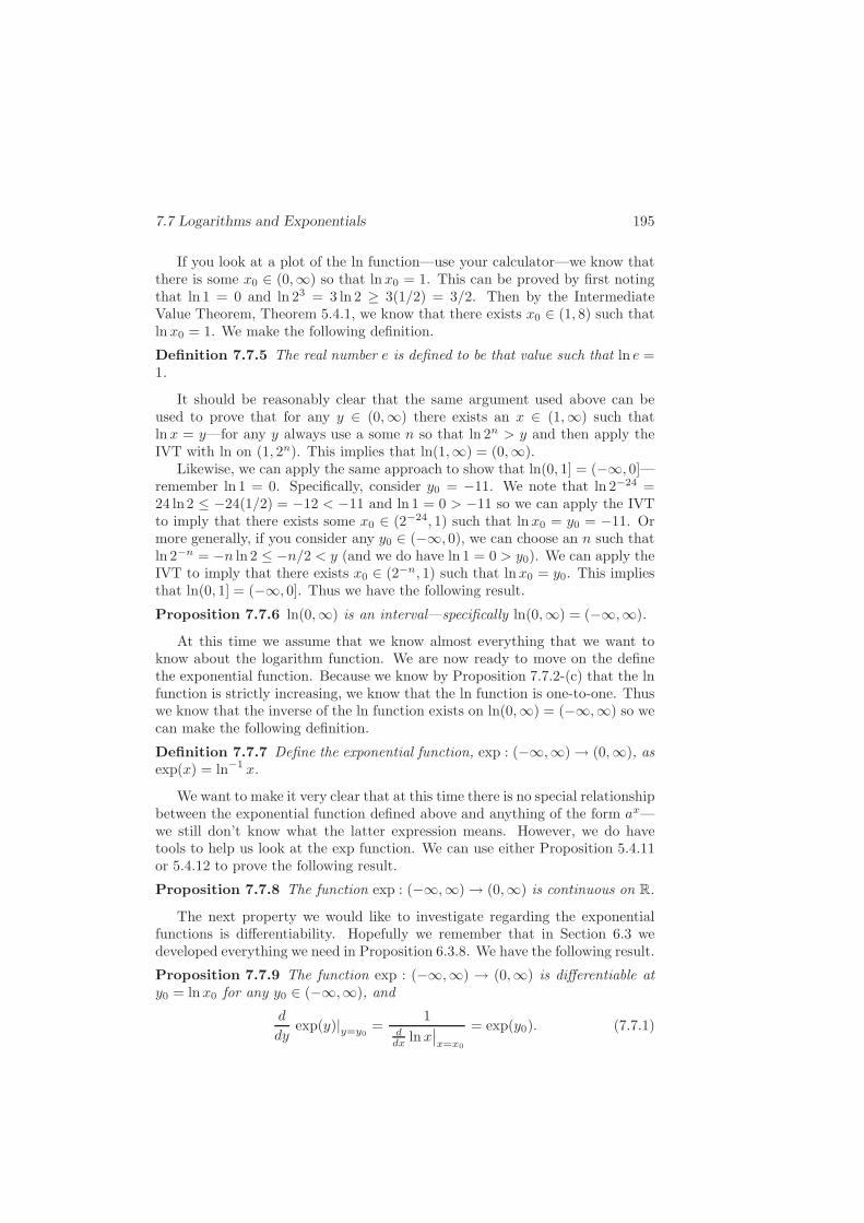
7.7 Logarithms and Exponentials 195
If you look at a plot of the ln function—use your calculator—we know thatthere is some x0 ∈ (0,∞) so that lnx0 = 1. This can be proved by first notingthat ln 1 = 0 and ln 23 = 3 ln 2 ≥ 3(1/2) = 3/2. Then by the IntermediateValue Theorem, Theorem 5.4.1, we know that there exists x0 ∈ (1, 8) such thatlnx0 = 1. We make the following definition.
Definition 7.7.5 The real number e is defined to be that value such that ln e =1.
It should be reasonably clear that the same argument used above can beused to prove that for any y ∈ (0,∞) there exists an x ∈ (1,∞) such thatlnx = y—for any y always use a some n so that ln 2n > y and then apply theIVT with ln on (1, 2n). This implies that ln(1,∞) = (0,∞).
Likewise, we can apply the same approach to show that ln(0, 1] = (−∞, 0]—remember ln 1 = 0. Specifically, consider y0 = −11. We note that ln 2−24 =24 ln2 ≤ −24(1/2) = −12 < −11 and ln 1 = 0 > −11 so we can apply the IVTto imply that there exists some x0 ∈ (2−24, 1) such that lnx0 = y0 = −11. Ormore generally, if you consider any y0 ∈ (−∞, 0), we can choose an n such thatln 2−n = −n ln 2 ≤ −n/2 < y (and we do have ln 1 = 0 > y0). We can apply theIVT to imply that there exists x0 ∈ (2−n, 1) such that lnx0 = y0. This impliesthat ln(0, 1] = (−∞, 0]. Thus we have the following result.
Proposition 7.7.6 ln(0,∞) is an interval—specifically ln(0,∞) = (−∞,∞).
At this time we assume that we know almost everything that we want toknow about the logarithm function. We are now ready to move on the definethe exponential function. Because we know by Proposition 7.7.2-(c) that the lnfunction is strictly increasing, we know that the ln function is one-to-one. Thuswe know that the inverse of the ln function exists on ln(0,∞) = (−∞,∞) so wecan make the following definition.
Definition 7.7.7 Define the exponential function, exp : (−∞,∞) → (0,∞), asexp(x) = ln−1 x.
We want to make it very clear that at this time there is no special relationshipbetween the exponential function defined above and anything of the form ax—we still don’t know what the latter expression means. However, we do havetools to help us look at the exp function. We can use either Proposition 5.4.11or 5.4.12 to prove the following result.
Proposition 7.7.8 The function exp : (−∞,∞) → (0,∞) is continuous on R.
The next property we would like to investigate regarding the exponentialfunctions is differentiability. Hopefully we remember that in Section 6.3 wedeveloped everything we need in Proposition 6.3.8. We have the following result.
Proposition 7.7.9 The function exp : (−∞,∞) → (0,∞) is differentiable aty0 = lnx0 for any y0 ∈ (−∞,∞), and
d
dyexp(y)|y=y0 =
1ddx lnx
∣
∣
x=x0
= exp(y0). (7.7.1)
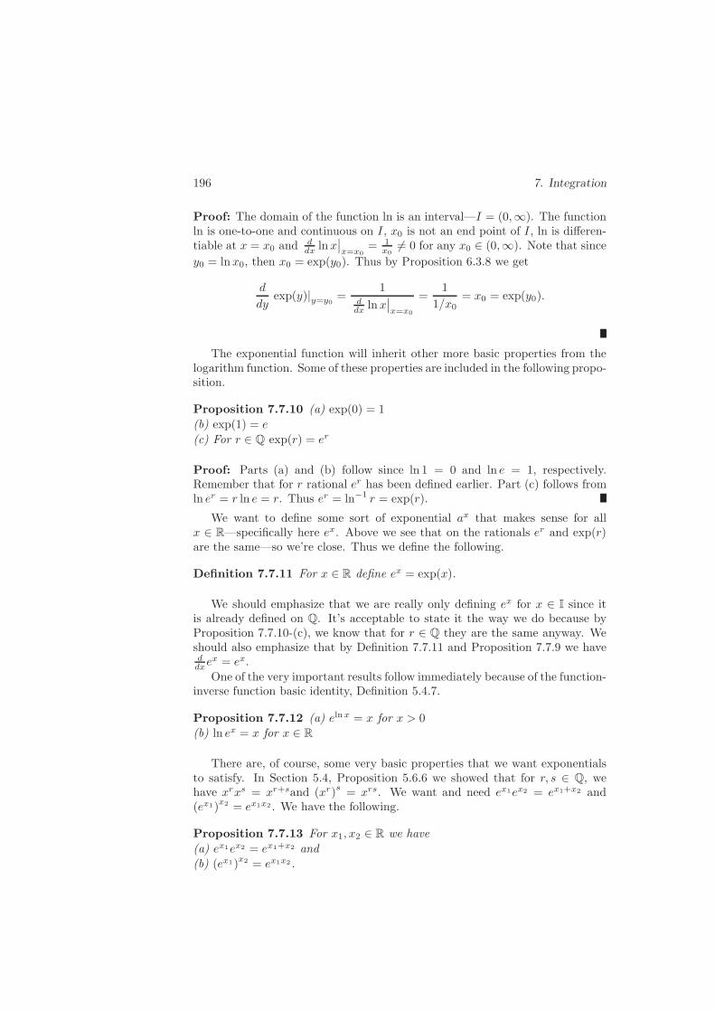
196 7. Integration
Proof: The domain of the function ln is an interval—I = (0,∞). The functionln is one-to-one and continuous on I, x0 is not an end point of I, ln is differen-tiable at x = x0 and d
dx lnx∣
∣
x=x0= 1
x06= 0 for any x0 ∈ (0,∞). Note that since
y0 = lnx0, then x0 = exp(y0). Thus by Proposition 6.3.8 we get
d
dyexp(y)|y=y0 =
1ddx lnx
∣
∣
x=x0
=1
1/x0= x0 = exp(y0).
The exponential function will inherit other more basic properties from thelogarithm function. Some of these properties are included in the following propo-sition.
Proposition 7.7.10 (a) exp(0) = 1
(b) exp(1) = e
(c) For r ∈ Q exp(r) = er
Proof: Parts (a) and (b) follow since ln 1 = 0 and ln e = 1, respectively.Remember that for r rational er has been defined earlier. Part (c) follows fromln er = r ln e = r. Thus er = ln−1 r = exp(r).
We want to define some sort of exponential ax that makes sense for allx ∈ R—specifically here ex. Above we see that on the rationals er and exp(r)are the same—so we’re close. Thus we define the following.
Definition 7.7.11 For x ∈ R define ex = exp(x).
We should emphasize that we are really only defining ex for x ∈ I since itis already defined on Q. It’s acceptable to state it the way we do because byProposition 7.7.10-(c), we know that for r ∈ Q they are the same anyway. Weshould also emphasize that by Definition 7.7.11 and Proposition 7.7.9 we haveddxe
x = ex.
One of the very important results follow immediately because of the function-inverse function basic identity, Definition 5.4.7.
Proposition 7.7.12 (a) elnx = x for x > 0
(b) ln ex = x for x ∈ R
There are, of course, some very basic properties that we want exponentialsto satisfy. In Section 5.4, Proposition 5.6.6 we showed that for r, s ∈ Q, wehave xrxs = xr+sand (xr)s = xrs. We want and need ex1ex2 = ex1+x2 and(ex1)
x2 = ex1x2 . We have the following.
Proposition 7.7.13 For x1, x2 ∈ R we have
(a) ex1ex2 = ex1+x2 and
(b) (ex1)x2 = ex1x2 .

7.7 Logarithms and Exponentials 197
Proof: This proposition could be proved using the same approach that we usedto prove Proposition 7.7.3. Instead of using that approach we will show howthese properties follow from results proved in Proposition 7.7.3. Suppose y1 andy2 are such that y1 = ex1 and y2 = ex2—then also x1 = ln y1 and x2 = ln y2.Then x1 + x2 = ln y1 + ln y2 = ln(y1y2) by Proposition 7.7.3-(a). Then takingthe exponential of both sides gives ex1+x2 = eln(y1y2) = y1y2 = ex1ex2 .
(b) In a similar way we note that x1x2 = x2 ln ex1 = ln (ex1)x2 . Then taking
the exponential of both sides yields ex1x2 = (ex1)x2 .
We do want and need more general exponentials. To accomplish this wemake the following definition.
Definition 7.7.14 For a > 0 and x ∈ R we define ax = ex ln a.
We next would have to state and prove all of the relevant properties relatedto the function ax. We want at least the following properties: a0 = 1, a1 = a,ax1ax2 = ax1+x2 , (ax1)x2 = ax1x2 and d
dxax = ax ln a. We will not prove
these properties but you should be able to see that they follow easily from theanalogous properties for the exponential—ex.
And finally we want one last very important function defined, xr for somer ∈ R and x ∈ (0,∞). The function xr is already defined, xr = er ln x. Of coursefor certain values of r (many values of r) we can actually define xr for any x ∈ R
(x2, x3, x2/3, etc)—but for many values of r (at least r = 1/2, r = π, etc) xr
just doesn’t make any sense for x < 0. And clearly the definition xr = er ln x
only makes sense for positive x.The most basic properties of xr follow from the properties of the exponential
and logarithm. We note that becuase lnxr = ln er ln x = r lnx, we see that now(essentially be definition) lnxr satisfies the property given in Proposition 7.7.3-(c)—this time for any r ∈ R (instead of only r ∈ Q).
The property that we need badly is the derivative property. We already havethat d
dxxr = rxr−1 for r ∈ Q. We also have the extension of this result.
Proposition 7.7.15 For r ∈ R and x ∈ (0,∞) ddxx
r = rxr−1.
Proof: We note that ddxx
r = ddxe
r ln x = er ln x rx = xr rx = rxr−1 which is the
desired result.
HW 7.7.1 (True or False and why) (a) ln 2n ≥ n2 implies that lim
n→∞ln 2n
(b) If ln 2x3 ln 8x = 1, then x = 110 .
(c) For x ∈ R,d
dxxx = (1 + lnx)xx.
(d) The function sinx x is defined only if x ∈ [0, 2π].(e) exp(lnx) = x for x > 0.
HW 7.7.2 Let f(θ) = cos θ. (a) Show that f is not one-to-one. Restrict f ina way so that the restriction, fr, is one-to-one.
(b) prove the existence of f−1r , prove the continuity of f−1
r and computed
dxf−1r (x),
i.e. computed
dxcos−1 x.

198 7. Integration
7.8 Improper Integrals
Two important assumptions made as a part of the definition of the integralwere that the functions were bounded and the interval was finite—and it’s easyto see that for many of the integration results proved, these were importantassumptions. However, there are many times that we want need some sortof integral of an unbounded function or some sort of integral over an infiniteinterval. In this section we introduce an extension of the integral to the improperintegral—an integral that allows for unbounded functions and infinite intervals.We want to emphasize that the integral considered in this section is not theDarboux-Riemann integral considered in the rest of the chapter.
We want a definition for integrals
∫ b
a
f where f may be unbounded at a, b
or at c ∈ (a, b). Likewise we want integrals of the form
∫ b
a
f where b is infinity,
a is minus infinity or both. We really do this by considering each possibilityseparate. To do this we make the following definition.
Definition 7.8.1 (a) Suppose that f : (a, b] → R is such that f is integrable on
[c, b] for any c ∈ (a, b]. Suppose further that lim c→ a+
∫ b
c
f exists. Then we
define
∫ b
a
f = limc→a+
∫ b
c
f .
(b) Suppose that f : [a, b) → R is such that f is integrable on [a, c] for any
c ∈ [a, b). Suppose further that lim c→ b−∫ c
a
f exists. Then we define
∫ b
a
f =
limc→b−
∫ c
a
f .
(c) Suppose that f : [a,∞) → R is such that f is integrable on [a, c] for any
c ∈ [a,∞). Suppose further that limc→∞
∫ c
a
f exists. Then we define
∫ ∞
a
f =
limc→∞
∫ c
a
f .
(d) Suppose that f : (−∞, b] → R is such that f is integrable on [c, b] for any
c ∈ (−∞, b]. Suppose further that lim c→ −∞∫ b
c
f exists. Then we define
∫ b
−∞f = lim
c→−∞
∫ b
c
f .
(e) Suppose that f : [a, c)∪ (c, b] → R is such that
∫ c
a
f and
∫ b
c
f exist and are
finite. Then we define
∫ b
a
f =
∫ c
a
f +
∫ b
c
f .
(f) Suppose that f : R → R is such that f is integrable on [−c1, c1] for every
c1 > 0. Then we define
∫ ∞
−∞f =
∫ c
−∞f +
∫ ∞
c
f for any c ∈ R.

Chapter 8
Sequences and Series
8.1 Approximation by Taylor Polynomials
The functions ex, sinx, 1√1−x2
, etc are nice functions—especially when you are
using a calculator or computer—but they are not as nice as polynomials. Specifi-cally polynomials can be evaluated completely based on multiplication, subtrac-tion and addition. Thus when you build your computer, if you teach it how tomultiply, subtract and add, your computer can also evaluate polynomials. Theseother functions are not that simple (even division creates problems). The waythat most computers evaluate the more complex functions is to approximatethem by polynomials.
There are many other applications where it is useful to have a polynomialapproximation to a function. Generally, polynomials are just easier to use. Inthis section we will show one way to obtain a polynomial approximation of afunction. The approximation will include the error term which is extremelyimportant since we must know that our approximation is a sufficiently goodapproximation—how good depends on our application. The main tool that wewill use is integration by parts, Proposition 7.5.6. We will use integration by
parts in the form
∫ b
a
F ′(t)G(t) dt = [FG]ba −
∫ b
a
F (t)G′(t) dt where we see that
it is convenient to include the variable of integration specifically because we willhave two variables in our formulas.
We consider a function f and desire to find a polynomial approximation off near x = a. At this time we will not worry about the necessary assumptionson our function—they will be included when we state our proposition. Webegin by noting that by the Fundamental Theorem of Calculus, Theorem 7.5.4,∫ x
a
f ′(t) dt = f(x) − f(a) or
f(x) = f(a) +
∫ x
a
f ′(t) dt. (8.1.1)
We write expression (8.1.1) as f(x) = T0(x) + R0(x) where T0(x) = f(a) and
199

200 8. Sequences and Series
R0(x) =∫ x
af ′(t) dt. T0 is referred to as the zero order Taylor polynomial of
the function f about x = a and R0 is the zero order error term—of course thetrivial case—and generally T0 would not be a very good approximation of f .
We obtain the next order of approximation by integrating
∫ x
0
f ′(t) dt by
parts. We let G(t) = f ′(t) and F ′(t) = 1. Then G′(t) = f ′′(t) and F (t) = t− c.You should take note of the last step carefully. The dummy variable in the
integral
∫ x
0
f ′(t) dt is t. Hence, if you were to integrate by parts without being
especially clever (or even sneaky), you would say that F = t. However, thereis no special reason that you could not use F = t + 1 or F = t + π instead.The only requirement is that the derivative of F with respect to t must be 1.Since the integration (and hence, the differentiation) is with respect to t, x is aconstant with respect to this operation (no different from 1, π or c). Since wewant it, it is perfectly ok to set F (t) = t − x. Then application of integrationby parts gives
∫ x
a
f ′(t) dt =
∫ x
a
F ′(t)G(t) dt = [FG]xa −
∫ x
a
F (t)G′(t) dt
= 0 − (a− x)f ′(a) −∫ x
a
(t− x)f ′′(t) dt = (x − a)f ′(a) −∫ x
a
(t− x)f ′′(t) dt.
If we plug this result into (8.1.1), we get
f(x) = f(a) + (x − a)f ′(a) −∫ x
a
(t− x)f ′′(t) dt. (8.1.2)
Expression (8.1.2) can be written as f(x) = T1(x) + R1(x) where T1(x) =f(a) + (x − a)f ′(a) is the first order Taylor polynomial of f at x = a and
R1(x) =
∫ x
a
(x− t)f ′′(t) dt is the first order error term. At this time it is not
clear that T1 is a better approximation of f than T0. You must be patient.
If we continue in the same fashion, we obtain the following result.
Proposition 8.1.1 Suppose f : I → R where I is some open interval contain-ing a and f is n + 1 times continuously differentiable on I. Then for x ∈ I fcan be written as
f(x) = Tn(x) +Rn(x) (8.1.3)
where
Tn(x) =n∑
k=0
1
k!f (k)(a)(x− a)k (8.1.4)
and
Rn(x) =1
n!
∫ x
a
(x− t)nf (n+1)(t) dt. (8.1.5)

8.1 Taylor Polynomials 201
The polynomial Tn is called the nth order Taylor polynomial of f about x = aand Rn is called the nth order Taylor error term.
Proof: We apply mathematical induction.Step 1: Equations (8.1.3)–(8.1.5) are true for n = 1 (by the derivation preceedingthis proposition).Step 2: Assume that equations (8.1.3)–(8.1.5) are true for n = m, i.e. assume
that f can be written as f(x) = Tm(x)+Rm(x) where Tm(x) =
m∑
k=0
1
k!f (k)(a)(x−
a)k and Rm(x) =1
m!
∫ x
a
(x− t)mf (m+1)(t) dt.
Step 3: We now prove that equations (8.1.3)–(8.1.5) are true for m + 1. Weintegrate the expression Rm by parts, letting G(t) = f (m+1)(t) and F ′(t) =1
m!(x − t)m and get
∫ x
a
1
m!(x− t)mf (m+1)(t) dt =
[
− 1
(m+ 1)!(x− t)m+1f (m+1)(t)
]t=x
t=a
−∫ x
a
[
− 1
(m+ 1)!(x − t)m+1f (m+2)(t)
]
dt
=1
(m+ 1)!(x− a)m+1f (m+1)(a)
+1
(m+ 1)!
∫ x
a
(x− t)m+1f (m+2)(t) dt.
Thus
Rm(x) =1
(m+ 1)!(x− a)m+1f (m+1)(a) +
1
(m+ 1)!
∫ x
a
(x− a)m+1f (m+2)(t) dt
and we can write
f(x) = Tm(x) +Rm(x) =
[
Tm(x) +1
(m+ 1)!(x− a)m+1f (m+1)(a)
]
+1
(m+ 1)!
∫ x
a
(x− t)m+1f (m+2)(t) dt
or f(x) = Tm+1(x) +Rm+1(x). Therefore equations (8.1.3)–(8.1.5) are true forn = m+ 1.
Therefore equations (8.1.3)–(8.1.5) are true for all n by mathematical induc-tion.
We note that if we choose a = 0 we obtain the following special case whichis very common.
Proposition 8.1.2 Suppose f : I → R where I is some open interval contain-ing 0 and f is n + 1 times continuously differentiable on I. Then for x ∈ I fcan be written as
f(x) = Tn(x) +Rn(x) (8.1.6)

202 8. Sequences and Series
where
Tn(x) =
n∑
k=0
1
k!f (k)(0)xk (8.1.7)
and
Rn(x) =1
n!
∫ x
0
(x− t)nf (n+1)(t) dt. (8.1.8)
We can consider the function f(x) = ex and can easily obtain expression forthe Taylor polynomial for f about x = 0.
Example 8.1.1 Obtain the Taylor polynomial and error term for f(x) = ex about x = 0.
Solution: It is easy to see that for any n, f(n)(0) = 1. Then we can write Tn(x) =n∑
k=0
1
k!xk
and Rn(x) =1
n!
∫ x
0(x − t)net dt.
Example 8.1.2 Consider the function f(x) =1
x + 1. Compute Taylor polynomials and
error terms for f about x = 2 for n = 4 and for general n.
Solution: We begin by making a table for derivatives of f at x = 2.
n f(n)(x) f(n)(2)
0 (x + 1)−1 3−1
1 −(x + 1)−2 −3−2
2 2!(x + 1)−3 2! · 3−3
3 −3!(x + 1)−4 −3! · 3−4
4 4!(x + 1)−5 4! · 3−5
5 −5!(x + 1)−6 −5! · 3−6
n (−1)nn!(x + 1)−(n+1) (−1)nn! · 3−(n+1)
n+1 (−1)n+1(n + 1)!(x + 1)−(n+2)
It is then easy to see that T4(x) =1
3− 1
9(x− 2) +
1
27(x− 2)2 − 1
81(x− 2)3 +
1
243(x− 2)4
and R4(x) = −5
∫ x
2(x − t)4(t + 1)−6 dt; and Tn(x) =
n∑
k=0
(−1)k 1
3k+1(x − 2)k and Rn(x) =
(−1)n+1(n + 1)
∫ x
2(x − t)n(t + 1)−(n+2) dt.
The title of this section was Approximation by Taylor Polynomials. Thefunction Tn does an especially good job of approximating f at x = a since Tnand the first n derivatives of Tn evaluated at x = a gives f(a) and the first nderivatives of f evaluated at x = a. For Tn to provide an approximation of ffor values of x other than x = a, it is clear that Rn will have to be small. If wethink about what a polynomial looks like, it is clear that a polynomial cannotapproximate a general function everywhere. To see how well Tn approximatesf , you might plot some of the Taylor polynomials found in Examples 8.1.1 and8.1.2 along with the given functions. The best that we can hope for is that Tnapproximates f near x = a—which we show with the following result which werefer to as the Taylor Inequality.
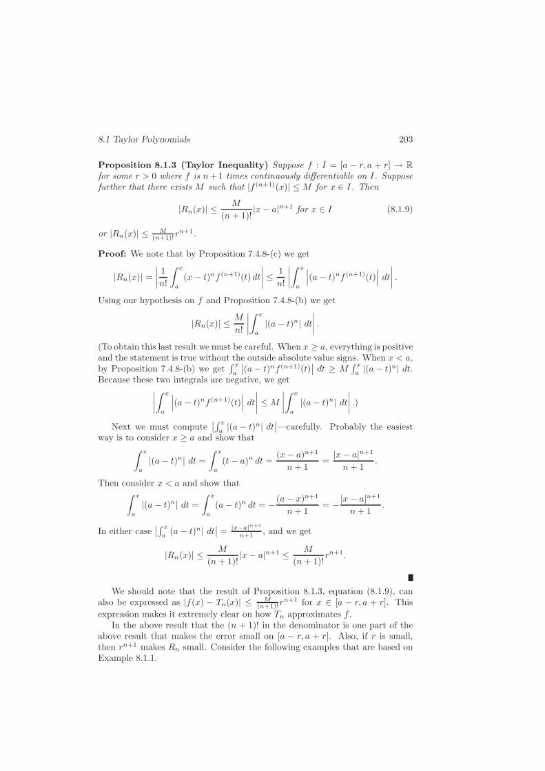
8.1 Taylor Polynomials 203
Proposition 8.1.3 (Taylor Inequality) Suppose f : I = [a − r, a + r] → R
for some r > 0 where f is n+1 times continuously differentiable on I. Supposefurther that there exists M such that |f (n+1)(x)| ≤M for x ∈ I. Then
|Rn(x)| ≤M
(n+ 1)!|x− a|n+1 for x ∈ I (8.1.9)
or |Rn(x)| ≤ M(n+1)!r
n+1.
Proof: We note that by Proposition 7.4.8-(c) we get
|Rn(x)| =
∣
∣
∣
∣
1
n!
∫ x
a
(x− t)nf (n+1)(t) dt
∣
∣
∣
∣
≤ 1
n!
∣
∣
∣
∣
∫ x
a
∣
∣
∣(a− t)nf (n+1)(t)
∣
∣
∣dt
∣
∣
∣
∣
.
Using our hypothesis on f and Proposition 7.4.8-(b) we get
|Rn(x)| ≤M
n!
∣
∣
∣
∣
∫ x
a
|(a− t)n| dt∣
∣
∣
∣
.
(To obtain this last result we must be careful. When x ≥ a, everything is positiveand the statement is true without the outside absolute value signs. When x < a,by Proposition 7.4.8-(b) we get
∫ x
a
∣
∣(a− t)nf (n+1)(t)∣
∣ dt ≥ M∫ x
a |(a− t)n| dt.Because these two integrals are negative, we get
∣
∣
∣
∣
∫ x
a
∣
∣
∣(a− t)nf (n+1)(t)
∣
∣
∣dt
∣
∣
∣
∣
≤M
∣
∣
∣
∣
∫ x
a
|(a− t)n| dt∣
∣
∣
∣
.)
Next we must compute∣
∣
∫ x
a |(a− t)n| dt∣
∣—carefully. Probably the easiestway is to consider x ≥ a and show that
∫ x
a
|(a− t)n| dt =
∫ x
a
(t− a)n dt =(x− a)n+1
n+ 1=
|x− a|n+1
n+ 1.
Then consider x < a and show that∫ x
a
|(a− t)n| dt =
∫ x
a
(a− t)n dt = − (a− x)n+1
n+ 1= −|x− a|n+1
n+ 1.
In either case∣
∣
∫ x
a(a− t)n| dt
∣
∣ = |x−a|n+1
n+1 , and we get
|Rn(x)| ≤ M
(n+ 1)!|x− a|n+1 ≤ M
(n+ 1)!rn+1.
We should note that the result of Proposition 8.1.3, equation (8.1.9), canalso be expressed as |f(x) − Tn(x)| ≤ M
(n+1)!rn+1 for x ∈ [a − r, a + r]. This
expression makes it extremely clear on how Tn approximates f .In the above result that the (n + 1)! in the denominator is one part of the
above result that makes the error small on [a − r, a + r]. Also, if r is small,then rn+1 makes Rn small. Consider the following examples that are based onExample 8.1.1.

204 8. Sequences and Series
Example 8.1.3 Return to Example 8.1.1.(a) Find the Taylor polynomial approximation of f(x) = ex associated with n = 3. Apply theTaylor inequaltiy, Proposition 8.1.3, with r = 3 to obtain an error bound on [−3, 3] for thisapproximation.(b) Repeat part (a) with r = 0.1.(c) Repeat part (a) with n = 27 and r = 3.
Solution: (a) We see that if we choose r = 3 and n = 3, then M = e3 ≈ 20.09, T3(x) =
1+x + 12x2 + 1
6x3 and by Proposition 8.1.3 |R3(x)| = |ex −T3(x)| ≤ e3
2434 ≈ 67.79 on [−3, 3].
This is not very good.
(b) If instead we choose r = .1 and n = 3, then M = e.1 ≈ 1.11, T3 is the same and
|R3(x)| = |ex − T3(x)| ≤ e.1
240.14 ≈ 4.60 · 10−6 on [−.1, .1]. These are very good results.
(c) If we want r = 3, we can choose n = 27 (or some other insanely large n), not write out T27
and see that |R27(x)| ≤ e3
28!328 ≈ 1.51 · 10−15. So if we especially want a large interval, it is
possible to find a sufficiently high order Taylor polynomial that will approximate f(x) = ex.
Thus we see that we can approximate ex well with a small order Taylorpolynomial on a small interval (with r small). It may not be very nice but wealso see that if for some reason we want or need a large interval, we can usea Taylor polynomial (a high ordered Taylor polynomial) to approximate ex onthe large interval.
Likewise we can revisit the example considered in Example 8.1.2, f(x) =1
x+1 , we clearly have to choose r so that −1 6∈ [2 − r, 2 + r]. If we choose
r = 1 and n = 4, then M = 5!1−6 ≈ 120 and |R4(x)| ≤ 5!1−6
5! 16 = 1 on theinterval [1, 3]—again not very good. If we instead chose r = 0.5 and n = 4,
then M = 5!1.5−6 ≈ 10.53 and |R4(x)| ≤ 5!1.5−6
5! .56 ≈ 1.37 · 10−3 on the interval[1.5, 2.5]. This is a much better result.
We see that in this case if r is a bit larger (1 or larger), M gets large—largeenough so that the (n + 1)! in the denominator of (8.1.9) doesn’t help makingR4 small. And of course, if r ≥ 1, the rn term doesn’t help make R4 smalleither.
HW 8.1.1 (True or False and why) (a) If n is sufficiently large and r is suffi-ciently small (but > 0), then Tn(x) = f(x) on [a− r, a+ r].(b) On any interval [a−r, a+r] the derivative f (n)(x) gets small as n gets larger.(c) A sufficient hypothesis for Proposition 8.1.1 is that each of the functionsf (k) be integrable, k = 1, · · · , k + 1.(d) If f is a fourth degree polynomial, then T4(x) = f(x) for all x ∈ R andR4(x) = 0 for all x ∈ R.(e) If Rn(x) = 0 for all x ∈ R and some n ∈ N, then f is a polynomial.
HW 8.1.2 Begin with f expressed as f(x) = T1(x) + R1(x) as in equation(8.1.2). Derive T2(x) and R2(x)—of course such that f(x) = T2(x) +R2(x).
HW 8.1.3 Consider the function f(x) = sinx. (a) Compute the Taylor poly-nomial and error term about x = 0 for n = 4 and for a general n.(b) Apply the Taylor inequality, Proposition 8.1.3, on [−1, 1] to determine abound on the error for both cases.

8.2 Sequences and Series 205
(c) Use the result from part (b) for general n to determine an n0 such that| sinx− Tn(x)| ≤ 1.0 · 10−10 for all x ∈ [−1, 1].
8.2 Sequences and Series
Convergence of sequences of functions In Proposition 8.1.3 we see thatif the function f is defined on [a − r, a + r], then |f(x) − Tn(x)| ≤ M
(n+1)!rn+1
where we worked to find M , n and r so that M(n+1)!r
n+1 is small. How small?
It depends on how accurately we want to approximate f .Hopefully that inequality above reminds you of convergence of sequences. If
we return to the function f(x) = ex and the sequence of Taylor polynomialsfound in Example 8.1.1, choose r = 3 and you plot f along with a bunch ofthe Tn’s for different n’s, it is clear that Tn converges to f by the Englishdefinition of ”converges”. For a fixed x ∈ [−3, 3] since by the Taylor inequality
− e3
(n+ 1)!3n+1 ≤ ex − Tn(x) ≤ e3
(n+ 1)!3n+1 and lim
n→∞3n+1
(n+ 1)!= 0 (Example
3.5.2), by the Sandwich Theorem, Proposition 3.4.2, we know that limn→∞
[ex −Tn(x)] = 0 or Tn(x) → f(x) = ex—for fixed x ∈ [−3, 3].
We formalize the concept of a sequence of functions converging to a givenfunction with the following defintions.
Definition 8.2.1 Suppose f, fn : D → R for D ⊂ R, n = 1, 2, · · · . If for eachx ∈ D lim
n→∞fn(x) exists and equals f(x), then we say that the sequence {fn}
converges pointwise to f on D. We write fn → f .
We have defined pointwise convergence of a sequence of functions. Thereother other types of convergence—we will include uniform convergence later.When there is no doubt that the convergence is pointwise, the ”pointwise” willoften be eliminated.
There are an abundant number of easy, important sequences of functions.Consider the following examples.
Example 8.2.1 Define f1n , f1 : D = [0, 1] → R for n ∈ N by
f1n (x) = xn and f1(x) =
{
0 for 0 ≤ x < 1
1 for x = 1.Show that f1n → f1 pointwise.
Solution: We note that
• since f1n (0) = 0 for all n, then f1n (0) → 0 = f1(0),
• for 0 < x < 1, since limn→∞
xn = 0 by Example 3.5.1, f1n (x) → 0 = f1(x), and
• since f1n (1) = 1 for all n, then f1n (1) → 1 = f1(1).
Thus f1n → f1 pointwise on [0, 1].
Example 8.2.2 Define f2n , f2 : [0, 1] → R for n ∈ N by f2n (x) = xn
nand f2(x) = 0 for
x ∈ [0, 1]. Show that f2n → f2 pointwise on [0, 1].
Solution: For any x ∈ [0, 1] limn→∞
xn
n= 0—thus f2n → f2 pointwise on [0, 1].

206 8. Sequences and Series
Example 8.2.3 Define f3n , f3 : [0, 1] → R for n ∈ N by f3n (x) =nx
1 + n2x2and f3(x) = 0
for x ∈ [0, 1]. Show that f3n → f3 pointwise on [0, 1].
Solution: Since f3n (0) = 0 for all n, then f3n (0) → 0 = f3(0). For x satisfying 0 < x ≤ 1,
limn→∞
nx
1 + n2x2= 0 = f3(x). Thus f3n → f3 pointwise on [0, 1].
Series We started this discussion talking about in which manner the Taylorpolynomial associated with f , Tn, converges to f . Specifically let Tn denotethe Taylor polynomial associated with f(x) = ex and consider the domainD = [−3, 3]. Earlier we found that lim
n→∞Tn(x) = ex for x ∈ [−3, 3]. Thus
the sequence {Tn} converges to ex pointwise on D = [−3, 3].It should be clear that {Tn} is a different sort of sequence from {f1n}, {f2n}
and {f3n} defined above. Recall that the sequence of Taylor polynomials Tn
associated with f(x) = ex is given by Tn(x) =
n∑
k=0
1
k!xk. All Taylor polynomials
look similar—given as a sum of n + 1 terms. When we take the limit as napproaches ∞, we are computing an infinite sum. We want to understand what
we mean by
∞∑
k=0
1
k!xk. Sequences such as these are referred to as a series of
functions. To provide a logical setting to discuss series of functions weintroduce series of real numbers.
For a sequence {a1, a2, · · · } where ai ∈ R for all i = 1, 2, · · · , we want to
discuss what we mean by∞∑
i=1
ai, the sum of an infinite number of real numbers.
We define partial sums of {ai} by sn =
n∑
i=1
ai for n ∈ N and consider the
sequence of partial sums, {sn}.
Definition 8.2.2 Consider the real sequence {ai} and the associated sequence
of partial sums {sn}, sn =n∑
i=1
ai. If the sequence {sn} is convergent, say to
s, we say that the series
∞∑
i=1
ai converges and we define
∞∑
i=1
ai = s = limn→∞
sn.
We refer to
∞∑
i=1
ai as an infinite series, or just a series. If the sequence {sn}
does not converge, we say that the series∞∑
i=1
ai does not converge. If sn → ±∞,
we say that the series
∞∑
i=1
ai diverges to ±∞, respectively—but make sure you
understand that a series that diverges to ±∞ does not converge in R.
Consider the following example.

8.2 Sequences and Series 207
Example 8.2.4 Consider the real series∞∑
i=1
ai where ai = ri for some r ∈ R. Then the
series∞∑
i=1
ai converges if and only if |r| < 1.
Solution: Recall that in Example 1.6.1 we showed that the formula for the sum of a finite
geometric series was given byn∑
j=0
Rj =1 − Rn+1
1 − R(where r was changed to R for convenience).
Applying this formula to the series given above gives formula for the partial sum sn =n∑
i=1
ri =
r1 − rn
1 − r. If r = 1, we use the fact that sn =
n∑
i=1
ri =n∑
i=1
1 = n to see that the sequence {sn}
diverges to infinity. When r 6= 1, limn→∞
sn exists if and only if limn→∞
rn exists. By Examples
3.2.6, 3.5.1, 3.6.2 and the discussion following Example 3.6.2 we know that limn→∞
rn exists if
and only if |r| < 1.
The geometric series is very nice but this is almost the only series that wecan write and work explicitly with the sequence of partial sums (telescopingseries gives one more example).
When we consider the convergence of a series, it is sometimes useful to realizethat when we are showing that sn → s where s is to be the sum of the series∞∑
i=1
ai, we must consider s−sn—as in |s−sn| < ǫ. And s−sn =
∞∑
i=n+1
ai. Thus
to show that a series converges, we must show that the sum of the ”tail end” ofthe series is arbitrarily small.
And finally one other approach is extremely useful when working with theconvergence of series is to use the Cauchy criterion for the convergence of thesequence {sn} introduced in Section 3.4. Recall that when we discussed theCauchy criterion, we noted that it was a case where we did not need to knowthe limit of the sequence. This is especially convenient when we are workingwith series in that we hardly ever know or can guess the sum of the series. Weinclude the application of the Cauchy criterion to the convergence of series inthe following proposition.
Proposition 8.2.3 Consider the real sequence {ai}. The series
∞∑
i=1
ai con-
verges if and only if for every ǫ > 0 there exists N ∈ R such that m,n ∈ N,
m ≥ n and m,n > N implies that
∣
∣
∣
∣
∣
m∑
i=n
ai
∣
∣
∣
∣
∣
< ǫ.
Proof: This result follows from Proposition 3.4.11 in that {sn} is convergentif and only if the sequence {sn} is a Cauchy sequence. The sequence {sn} is aCauchy sequence if for every ǫ > 0 there exists an N ∈ R such that n,m ∈ N
and n,m > N implies |sm − sn| < ǫ. This can easily be adjusted by settingN∗ = N +1 and requiring m,n > N∗ which implies that |sm−sn−1| < epsilon.

208 8. Sequences and Series
If we take m ≥ n (one of the two must be larger), then sm − sn−1 =∑m
i=n ai.The result follows.
We used the example of convergence of Taylor polynomials to motivate theconvergence of series. We now realize that the convergence of Taylor polynomialsare really the convergence of a series, a Taylor series. For that reason (and thefact that it is an important concept) we now define what we mean by thepointwise convergence of a series of functions.
Definition 8.2.4 Consider the sequence of functions {fi(x)} where for each i,
fi : D → R, D ⊂ R. If for each x ∈ D the real series
∞∑
i=1
fi(x) is convergent, say
to s(x), then we say that the series of functions
∞∑
i=1
fi(x) converges pointwise
to s(x).
Begin by noting that the notation used above is not very good. At the function
level it would be better to say that the series of functions
∞∑
i=1
fi converges
pointwise to s—but the above notation is reasonably common.We should note that we can also consider the sequence of partial sums of
functions, sn(x) =∑ni=1 fi(x), and say that if the sequence {sn(x)} converges
pointwise, say to s(x), then the series of functions
∞∑
i=1
fi(x) is said to converge
pointwise and is defined to be equal to s(x).
In our consideration of the convergence of sequences of Taylor polynomialswe have already given a very common example of a series of functions. SinceTn(x) was really a partial sum, when we considered the convergence of the Taylorpolynomials of f(x) = ex on [−3, 3], we were proving the pointwise convergence
of the series of functions∞∑
i=0
1
i!xi (and we hope that you realize that it is not
important that we considered general series starting at i = 1 and the Taylorseries started with i = 0). Because we expanded f(x) = ex about x = 0, theseries given above is the Maclaurin series of f . In general we make the followingdefintiion.
Definition 8.2.5 Let I be a neighborhood of x = a and suppose f : I → R has
derivatives of all orders at x = a. Then
∞∑
k=0
f (k)(a)
k!(x− a)k is called the Taylor
series expansion of f about x = a. When a = 0, the Taylor series is most oftenreferred to as the Maclaurin series.
HW 8.2.1 Prove that the sequence of functions {fn} where fn : [0, 1] → R isdefined by fn(x) = nx(1− x2)n converges to f where f(x) = 0 for all x ∈ [0, 1].
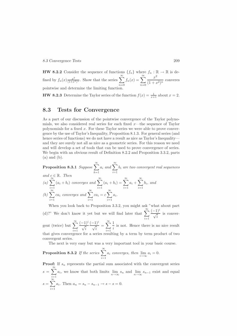
8.3 Convergence Tests 209
HW 8.2.2 Consider the sequence of functions {fn} where fn : R → R is de-
fined by fn(x)x2
(1+x2)n . Show that the series∞∑
n=0
fn(x) =∞∑
n=0
x2
(1 + x2)nconveres
pointwise and determine the limiting function.
HW 8.2.3 Determine the Taylor series of the function f(x) = 1x+1 about x = 2.
8.3 Tests for Convergence
As a part of our discussion of the pointwise convergence of the Taylor polyno-mials, we also considered real series for each fixed x—the sequence of Taylorpolynomials for a fixed x. For these Taylor series we were able to prove conver-gence by the use of Taylor’s Inequality, Proposition 8.1.3. For general series (andhence series of functions) we do not have a result as nice as Taylor’s Inequality—and they are surely not all as nice as a geometric series. For this reason we needand will develop a set of tools that can be used to prove convergence of series.We begin with an obvious result of Definition 8.2.2 and Proposition 3.3.2, parts(a) and (b).
Proposition 8.3.1 Suppose∞∑
k=1
ai and∞∑
i=1
bi are two convergent real sequences
and c ∈ R. Then
(a)
∞∑
i=1
(ai + bi) converges and
∞∑
i=1
(ai + bi) =
∞∑
i=1
ai +
∞∑
i=1
bi, and
(b)
∞∑
i=1
cai converges and
∞∑
i=1
cai = c
∞∑
i=1
ai.
When you look back to Proposition 3.3.2, you might ask ”what about part
(d)?” We don’t know it yet but we will find later that
∞∑
i=1
(−1)i√i
is conver-
gent (twice) but∞∑
i=1
(−1)i√i
(−1)i√i
=∞∑
i=1
1
iis not. Hence there is no nice result
that gives convergence for a series resulting by a term by term product of twoconvergent series.
The next is very easy but was a very important tool in your basic course.
Proposition 8.3.2 If the series∞∑
i=1
ai converges, then limi→∞
ai = 0.
Proof: If sn represents the partial sum associated with the convergent series
s =
∞∑
i=1
ai, we know that both limits limn→∞
sn and limn→∞
sn−1 exist and equal
s =
∞∑
i=1
ai. Then an = sn − sn−1 → s− s = 0.

210 8. Sequences and Series
As we said earlier, the result given in Proposition 8.3.2 is very important—but not in the form given in Proposition 8.3.2. For this reason we state thecontrapositive of Proposition 8.3.2 as the following corollary—called the ”testfor divergence” in the basic course.
Corollary 8.3.3 Test for Divergence Consider the series
∞∑
i=1
ai. If limi→∞
ai 6=
0, then the series
∞∑
i=1
ai does not converge.
One thing that we want to emphasize is that the statement ” limi→∞
ai 6= 0 can
be satisfied if either the limit does not exist, or the limit exists and is not equal
to zero. Of course this corollary can be used to show that the series
∞∑
i=1
(−1)i,
∞∑
i=1
2i and∞∑
i=1
sin(i) do not converge. We do not know it yet but the series∞∑
i=1
1
i
does not converge. For this series ai = 1/i → 0. Hence we emphasize that theconverse of Proposition 8.3.2 is not true.
We next include a concept that will be very important to us later. We beginby including the definition of absolute and conditional convergence.
Definition 8.3.4 Suppose {ai} is a real sequence. We say that {ai} is abso-
lutely convergent if the series∞∑
i=1
|ai| is convergent. If the series {ai} is con-
vergent but not absolutely convergent, then the series is said to be conditionallyconvergent.
We then state and prove the following result.
Proposition 8.3.5 Suppose {ai} is a real sequence. If the series∞∑
i=1
ai is ab-
solutely convergent, then it is convergent.
Proof: This is one of the results where it is very convenient to consider theCauchy criterion for the convergence of a series given in Proposition 8.2.3. We
suppose that we are given an ǫ > 0. Since
∞∑
i=1
ai is absolutely convergent, we
know that there exists N ∈ R such that n,m ∈ N, n,m > N and m > n (for
convenience) implies
∣
∣
∣
∣
∣
m∑
i=n
|ai|∣
∣
∣
∣
∣
< ǫ (where the outer absolute value signs are not
really needed). Then m,n ∈ N, m,n > N and m > n implies—by multipleapplications of the triangular inequality, Proposition 1.5.8-(v), or an easy math

8.3 Convergence Tests 211
induction proof—
∣
∣
∣
∣
∣
m∑
i=n
ai
∣
∣
∣
∣
∣
≤m∑
i=n
|ai| < ǫ. Thus by the Cauchy criterion for
convergence of series the series
∞∑
i=1
ai converges.
We see that if we consider the series
∞∑
i=1
1
2i, which we know is convergent
because it is a geometric series associated with r = 1/2 < 1, then we immediately
know that the series
∞∑
i=1
(−1)i1
2iis convergent—or any other series like this
where some of the terms are negative. We will apply this result often in asimilar way.
The series results given so far do not directly help us decide whether ornot series converge. When we worked with sequences, we had many methodsthat helped find limits. We next state and proof a series of results that helpdetermine whether or not a series is convergent. We begin with the integral test(recall that we considered improper integrals in Section 7.8).
Proposition 8.3.6 (Integral Test) Suppose that
∞∑
i=1
ai is a real series and
suppose f : [1,∞) is a positive, decreasing continuous function for which f(i) =
ai for i ∈ N. Then
∞∑
i=1
ai converges if and only if the integral
∫ ∞
1
f exists.
Proof: Before we proceed we emphasize that we are assuming that
∫ ∞
1
f
exists in R (we do not include convergence to ∞ for this assumption). Since fis decreasing on the interval [i − 1, i], we know that f(i − 1) ≥ f(t) ≥ f(i) for
any t ∈ [i−1, i]. Hence by Proposition 7.4.5, f(i−1) =
∫ i
i−1
f(i−1) ≥∫ i
i−1
f ≥∫ i
i−1
f(i) = f(i), or ai−1 ≥∫ i
i−1
f ≥ ai. If we sum from i = 2 to i = n and
apply Proposition 7.4.3, we get
sn−1 ≥∫ n
1
f ≥ sn − a1. (8.3.1)
(⇒) We assume s =
∞∑
i=1
ai converges. Since ai ≥ 0 for all i, the left side of
inequality (8.3.1) yields
∫ n
1
f ≤ sn−1 ≤∞∑
i=1
ai = s. Therefore, the sequence
{
bn =
∫ n
1
f
}
is a bounded, monotone increasing sequence. By the Monotone

212 8. Sequences and Series
Convergence Theorem, Theorem 3.5.2-(a), the limit limn→∞
bn = limn→∞
∫ n
1
f exists
and equals L = lub{bn : n ∈ N}. Because L ≥ bn for any n, the convergenceof the sequence {bn} can be expressed as follows: for every ǫ > 0 there existsN ∈ R such that n > N implies that |bn − L| = L− bn < ǫ.
The above limit is not enough to show that the improper integral
∫ ∞
1
f
exists. We must show that limR→∞
∫ R
1
f exists. We claim that this limit does in
fact exist and will equal L. Suppose that ǫ > 0 is given. Choose the N basedon the convergence of the sequence {bn}. Let N1 = N + 1 and suppose thatR > N1. Note that since f(x) ≥ 0, we can use Propositions 7.3.3 and 7.4.5
to show that
∫ R
1
f ≥∫ [R]
1
f where [R] is the greatest integer function. Then
[R] > N and
∣
∣
∣
∣
∣
L−∫ R
1
f
∣
∣
∣
∣
∣
= L−∫ R
1
f ≤ L−∫ [R]
1
f =∣
∣b[R] − L∣
∣ < ǫ.
Therefore limR→∞
∫ R
1
f exists and the improper integral
∫ ∞
1
f exists.
(⇐) We now assume that the integral
∫ ∞
1
f exists. By the right side of in-
equality (8.3.1), the fact that f is positive and the fact that
∫ ∞
1
f exists, we
see that sn − a1 ≤∫ n
1
f ≤∫ ∞
1
f—the sequence {sn − a1} is bounded. Since
ai ≥ 0 for all i, the sequence {sn} is increasing—so the sequence {sn−a1} is alsoincreasing. Thus by the Monotone Convergence Theorem, Theorem 3.5.2-(a),the sequence {sn−a1} is convergent. Thus the sequence {sn} is also convergent
(using Proposition 3.3.2-(a)) and the series
∞∑
i=1
ai converges.
The form of the integral test given in Proposition 8.3.6 is not in the formthat we are accustomed to using. We rewrite Proposition 8.3.6 in the followingcorollary where we include one of the implications from Proposition 8.3.6 andthe contrapositive of the other implication from Proposition 8.3.6.
Corollary 8.3.7 (Integral Test) Suppose that
∞∑
i=1
ai is a real series and sup-
pose f : [1,∞) is a positive, decreasing continuous function for which f(i) = aifor i ∈ N.
(a) If the improper integral∫∞1 f exists, then the series
∞∑
i=1
ai is convergent.
8.3 Convergence Tests 213
(b) If the improper integral∫∞1f does not exist, then the series
∞∑
i=1
ai is not
convergent.
The integral test is a specially good result because it gives us a large number
of convergent sequences easily. It is easy to see that
∫ ∞
1
1
xpexists for p > 1 and
does not exist for p ≤ 1. Thus we get the p-series:∞∑
i=1
1
ipconverges for p > 1
and diverges if p ≤ 1. There are some other series on which the integral test canbe used but not many important ones. We also note at this time that if we applythe idea of absolute convergence along with some of these p-series, we obtain
more convergent series. We see that since∞∑
i=1
1
i3converges, then
∞∑
i=1
(−1)i1
i3
also converges. Of course we can find many more convergent series using thismethod.
The next result, the comparison test, is important but is often difficult touse.
Proposition 8.3.8 (Comparison Test) Suppose that {ai} and {bi} are real,positive sequences and suppose that for some N1 ∈ N ai ≤ bi for all i ≥ N1. If
the series∞∑
i=1
bi converges, then the series∞∑
i=1
ai converges.
Proof: Since
∞∑
i=1
bi converges, we know from Proposition 8.2.3 that for every
ǫ > 0 there exists an N2 ∈ R such that n,m ∈ N, n,m > N2 and m > n
implies thatm∑
i=n
bi < ǫ (where no absolute value signs are needed since {bi} was
assumed to be a positive series). If we then let N = max{N1, N2}, we know
that for n,m ∈ N, n,m > N and m > n we havem∑
i=n
ai ≤m∑
i=n
bi < ǫ. Therefore
again by Proposition 8.2.3 we know that
∞∑
i=1
ai converges.
We mentioned earlier that the comparison test is often difficult to use. If we
consider a series such as∞∑
i=1
1
i2 + i+ 1, it is easy to see that
1
i2 + i+ 1≤ 1
i2.
∞∑
i=1
1
i2converges because it is a p-series with p = 2. Hence, by the comparison
test
∞∑
i=1
1
i2 + i+ 1converges.

214 8. Sequences and Series
If we instead consider a series such as∞∑
i=1
1
i2 − i+ 1we have to be more
clever. We note that i2−i+1 ≥ i2−2i+1 = (i−1)2, then1
(i− 1)2≥ 1
i2 − i+ 1
for i ≥ 2. The series
∞∑
i=2
1
(i− 1)2is a p-series with p = 2 so it is convergent—
it is not exactly in the form of a p-series but it should be clear that with achange of variable j = i − 1, we see that it is exactly in the form of a p-series.
Then by the Comparsion Test,
∞∑
i=1
1
i2 − i+ 1is convergent. We note that the
series in Proposition 8.3.8 both start at i = 1 where in this example the series∞∑
i=2
1
(i− 1)2starts at i = 2. This is no problem. We could add an i = 1 term,
say b1 = 13. The series 13+
∞∑
i=2
1
(i− 1)2will still be convergent and Proposition
8.3.8 will apply with N1 = 2.
Just as we did following the integral test, we can apply the comparison testin conjunction with absolute convergence. Using the comparison test and the
fact that| sin i|i2
≤ 1
i2, it is easy to see that the series
∞∑
i=1
| sin i|i2
is convergent.
Then using Proposition 8.3.5 we know that
∞∑
i=1
sin i
i2converges.
The next convergence test is an extremely nice result that takes care of mostof the difficulties associated with the comparison test.
Proposition 8.3.9 (Limit Comparison Test) Suppose that {ai} and {bi}are positive, real sequences.
(a) If limn→∞
aibi
6= 0, then the series
∞∑
i=1
ai is convergent if and only if the series
∞∑
i=1
bi is convergent. Note that (a) can be worded as follows:
(a1) If limi→∞
aibi
6= 0 and∞∑
i=1
bi converges, then∞∑
i=1
ai converges, and
(a2) If limn→∞
aibi
6= 0 and
∞∑
i=1
bi does not converge, then
∞∑
i=1
ai does not converge.
(b) If limn→∞
aibi
= 0 and
∞∑
i=1
bi converges, then
∞∑
i=1
ai converges.
Proof: The statement of the proposition above really consists of parts (a) and(b). Parts (a1) and (a2) are rewordings of part (a)—one implication and the

8.3 Convergence Tests 215
contrapositive of the other implication. Statements (a1) and (a2) are in a formmuch easier to apply than that of (a).
(a) (⇒) We assume that limi→∞
aibi
= r 6= 0 and the series
∞∑
i=1
ai is convergent.
Since ai and bi are positive, r > 0. Because limi→∞
aibi
= r > 0, for every ǫ > 0
there exists N ∈ R such that i > N implies that
∣
∣
∣
∣
aibi
− r
∣
∣
∣
∣
< ǫ or
r − ǫ <aibi< r + ǫ. (8.3.2)
Since the sequence {bi} is assumed positive, inequality (8.3.2) can be rewrittenas
(r − ǫ)bi < ai < (r + ǫ)bi. (8.3.3)
Choose ǫ = r/2. Then for i > N we have (r/2)bi < ai. By the comparison test,
Proposition 8.3.8, since
∞∑
i=1
ai converges,
∞∑
i=1
(r/2)bi converges. By Proposition
8.3.1-(b) this implies that
∞∑
i=1
bi is also convergent.
(⇐) The proof of this directions is almost identical to the previous proof. Thedifference is that this time, the right hand half of inequality (8.3.3) is used
along with the comparison test to show that if∞∑
i=1
bi converges, then∞∑
i=1
ai is
also convergent—try it.
(b) If limn→∞
aibi
= 0, then for ǫ > 0 there exists an N ∈ R such that i > N implies
thataibi< ǫ (no absolute value signs are necessary because both sequences are
positive). Thus for i > N we have
ai < ǫbi. (8.3.4)
Thus by the Proposition 8.3.1-(b) and the comparison test, the convergence of∞∑
i=1
bi implies the convergence of∞∑
i=1
ai.
Hopefully you remember from your basic course that you can easily prove the
convergence of
∞∑
i=1
1
i2 − i+ 1by setting ai =
1
i2 − i+ 1, bi =
1
i2and applying
part (a1) of the limit comparison test (realizing that
∞∑
i=1
bi converges because it
is a p-series with p = 2). This is much easier than applying the comparison test.
To show that
∞∑
i=1
i2 + i+ 1
i3 + i2 + i+ 1does not converge, we set ai =
i2 + i+ 1
i3 + i2 + i+ 1,
216 8. Sequences and Series
bi =1
i, show that
aibi
→ 1 as i→ ∞, and apply part (a2) of the limit comparison
test to see that
∞∑
i=1
i2 + i+ 1
i3 + i2 + i+ 1does not converge (recall that
∞∑
i=1
1
idiverges
since it is a p-series with p = 1).
Generally, the limit comparison test allows you to prove the comvergence ordivergence of a series by ”comparing” the series with a known much nicer seriesthat is similar to the original series—similar in that the limit ai/bi → r exists.
We next introduce the convergence test that might be the most importanttest of them all. The ratio test is applicable on series that are almost geometricseries—as we shall see by the proof and the examples that follow. Of course theratio test will work on a geometric series but we don’t need it there.
Proposition 8.3.10 Ratio Test Consider a real sequence of non-zero ele-ments {ai}.(a) Suppose that there exists r, 0 < r < 1, and an N ∈ N such that i ≥ N
implies that
∣
∣
∣
∣
ai+1
ai
∣
∣
∣
∣
≤ r. Then the series∞∑
i=1
ai is absolutely convergent.
(b) Suppose that there exists r, r ≥ 1, and an N ∈ N such that i ≥ N implies
that
∣
∣
∣
∣
ai+1
ai
∣
∣
∣
∣
≥ r. Then the series
∞∑
i=1
ai does not converge.
Proof: (a) Suppose that there exists r, 0 < r < 1 and an N ∈ N such that
i ≥ N implies that
∣
∣
∣
∣
ai+1
ai
∣
∣
∣
∣
≤ r. Note the following.
•∣
∣
∣
∣
aN+1
aN
∣
∣
∣
∣
≤ r implies that |aN+1| ≥ r|aN |
•∣
∣
∣
∣
aN+2
aN+1
∣
∣
∣
∣
≤ r implies that |aN+2| ≤ r|aN+1| ≤ r2|aN |
• Claim: m ≥ 1 implies that |aN+m| ≤ rm|aN |Proof by mathematical induction
Step 1: True for m = 1, given above.
Step 2: Assume true for m = k, i.e. assume that |aN+k| ≤ rk|aN |.
Step 3: Since
∣
∣
∣
∣
aN+k+1
aN+k
∣
∣
∣
∣
≤ r, |aN+k+1| ≤ r|aN+k| ≤ rrk|aN | (by the
inductive hypothesis). Thus |aN+k+1| ≤ rk+1|aN |, i.e. it is true for m =k + 1.
Therefore by math induction the statement is true for allm, i.e. form ≥ 1,|aN+m| ≤ rm|aN |.

8.3 Convergence Tests 217
We know that the series∞∑
m=1
rm+1|aN | is convergent since it is a geometric
series. By the comparison test we then know that
∞∑
m=1
aN+m is convergent. And
finally, sinceN∑
i=1
ai is a finite sum, we then know thatN∑
i=1
ai+∞∑
m=1
aN+m =∞∑
i=1
ai
is convergent.
(b) Suppose that there exists r, r ≥ 1 and an N ∈ N such that i ≥ N implies
that
∣
∣
∣
∣
ai+1
ai
∣
∣
∣
∣
≥ r. By a mathematical induction proof similar to that used in
part (a) we can show that m ≥ 1 implies that |aN+m| ≥ rm|aN |. Since r ≥ 1,it is clear that |aN+m| 6→ 0 as m → ∞. Thus it is impossible that aN+m → 0(because if aN+m → 0, then |aN+m| → 0). And if aN+m 6→ 0, it should be clear
that ai 6→ 0. Thus by Corollary 8.3.3 we know that the series
∞∑
i=1
ai does not
converge.
We should note that the above version of the ratio test is not the versionusually included in the basic calculus texts. We include the following version ofthe ratio test.
Corollary 8.3.11 Ratio Test Consider a real sequence of non-zero elements
{ai}. Suppose that limi→∞
∣
∣
∣
∣
ai+1
ai
∣
∣
∣
∣
= r. Then
(a) if r < 1, then the series
∞∑
i=1
ai is absolutely convergent.
(b) if r > 1, then the series
∞∑
i=1
ai is not convergent.
(c) if r = 1, then no prediction can be made.
Proof: (a) If limi→∞
∣
∣
∣
∣
ai+1
ai
∣
∣
∣
∣
= r < 1, for every ǫ > 0 there exists N ∈ R such that
n > N implies that
∣
∣
∣
∣
∣
∣
∣
∣
ai+1
ai
∣
∣
∣
∣
− r
∣
∣
∣
∣
< ǫ. Choose ǫ = (1−r)/2 and set N1 = [N ]+1.
Then for n ≥ N1 we have 0 <
∣
∣
∣
∣
ai+1
ai
∣
∣
∣
∣
< r +1 − r
2=r + 1
2< 1. Thus by part
(a) of Proposition 8.3.10 the series
∞∑
i=1
ai converges.
(b) Again we know that for every ǫ > 0 there exists N ∈ R such that i > N
implies that
∣
∣
∣
∣
∣
∣
∣
∣
ai+1
ai
∣
∣
∣
∣
− r
∣
∣
∣
∣
< ǫ—but now r > 1. Choose ǫ = (r − 1)/2 and set
N1 = [N ] + 1. Then for i ≥ N1 we have 1 <r + 1
2< r − r − 1
2<
∣
∣
∣
∣
ai+1
ai
∣
∣
∣
∣
. Thus

218 8. Sequences and Series
we can use part (b) of Proposition 8.3.10 to see that the series∞∑
i=1
ai does not
converge.
(c) If we consider
∞∑
i=1
1
i, we see that lim
i→∞
∣
∣
∣
∣
1/(i+ 1)
1/i
∣
∣
∣
∣
= 1 and we know that the
series∞∑
i=1
1
idoes not converge. If we consider
∞∑
i=1
1
i2, we see that lim
i→∞
∣
∣
∣
∣
1/(i+ 1)2
1/i2
∣
∣
∣
∣
=
1 and we know that the series
∞∑
i=1
1
i2converges. Hence the condition that r = 1
does not determine whether or not a series converges.
Notice that as a part of the proofs of parts (a) and (b) we had to do a danceto make for the point that we only require the ”N” in the definition of a limit ofa sequence to be in R—using N1 = [N ] + 1 when we needed an integer. Therewere times when it was convenient to allow N to be any real number that works.In the above proof we had to pay for that earlier convenience.
Another well known test is the root test. At times the root test is clearly thenatural test to use. In most other cases the root test is very difficult to apply.We state the following result.
Proposition 8.3.12 (Root Test) Consider a real sequence {ai}.(a) Suppose that there exists r, 0 < r < 1, and an N ∈ N such that i ≥ N
implies that |ai|1/i ≤ r. Then the series
∞∑
i=1
ai is absolutely convergent.
(b) Suppose that there exists r, r ≥ 1, and an N ∈ N such that i ≥ N implies
that |ai|1/i ≥ r. Then the series
∞∑
i=1
ai does not converge.
Proof: (a) If |ai|1/i ≤ r for i ≥ N , then |ai| ≤ ri. Then since∑∞
i=1 ri converges
(it is a geometric series and r < 1), the series
∞∑
i=1
|ai| converges—of course we
really get that the tail end of the series converges (from N on) which impliesthat the whole series converges.
(b) Since |ai|1/i ≥ r, we have |ai| ≥ ri. Then since r ≥ 1, we know that|ai| 6→ 0 which implies that ai 6→ 0—which by Corollary 8.3.3 implies that the
series
∞∑
i=1
ai does not converge.
We should note that like the ratio test, the statement of Proposition 8.3.12is not the version that is usually given in basic calculus texts. And as was thecase with the ratio test, the more tradition root test will follow from Proposition8.3.12.
There is one more important test for convergence that we must consider.We should realize that until this time all of our tests were for positive series

8.3 Convergence Tests 219
or they gave absolute convergence (ratio and root test). The only way that weproved convergence of series that was not positive was to use Proposition 8.3.5—absolute convergence implies convergence. We next consider a class of series thatare not positive called alternating series. We now include the following definitionand the associated convergence theorem.
Definition 8.3.13 Consider a real sequence of positive elements {ai}. The
series
∞∑
i=1
(−1)i+1ai is said to be an alternating series.
Note that we set the exponent on the −1 term to be i+ 1 just so that the firstterm would be positive—that seems a bit neater. This is not important. It isstill an alternating series if it starts out negative and the result given below isequally true for alternating series that start with a negative term.
Proposition 8.3.14 (Alternating Series Test) Consider the real, positivedecreasing sequence of elements {ai} and suppose that lim
i→∞ai = 0. Then the
alternating series
∞∑
i=1
(−1)iai converges.
Proof: Consider the sequence of partial sums s2n = (a1 − a2) + (a3 − a4) +· · ·+ (a2n−1 − a2n). Since ak − ak+1 ≥ 0, the sequence is increasing. Also sinceak − ak+1 ≥ 0, k = 2, · · · , 2n− 2, and a2n > 0,
s2n = a1 − (a2 − a3) − (a4 − a5) − · · · − (a2n−2 − a2n−1) − a2n ≤ a1,
i.e. the sequence {s2n} is bounded above. Then by the Monotone ConvergenceTheorem, Theorem 3.5.2-(a), the sequence {s2n} converges—say to s. Thensince s2n+1 = s2n + a2n+1 and the fact that a2n+1 → 0, we see that {s2n+1}also converges to s.
Claim: The sequence {sn} converges to s. Let ǫ > 0 be given and letN1 be such that n > N1 implies that |s2n − s| < ǫ, i.e. if 2n > 2N1, then|s − s2n| < ǫ. Let N2 be such that n > N2 implies that |s − s2n+1| < ǫ, i.e. if2n+ 1 > 2N2 + 1, then |s− s2n+1| < ǫ.
Then if we define N = max{2N1, 2N2+1}, then n > N implies that |s−sn| <
ǫ, so limn→
sn = s or the series
∞∑
i=1
(−1)iai converges—to s.
We emphasize here that to apply the alternating series test we must showthat the sequence is (i) decreasing, (ii) ai → 0 and that (iii) the series is alter-
nating. We used the fact earlier that the series
∞∑
i=1
(−1)i√i
converges. It is easy
to see that (i) ai+1 =1√i+ 1
<1√i
= ai (which is the same as√i <
√i+ 1 or

220 8. Sequences and Series
i < i+ 1), and (ii) limi→∞
1√i
= 0. Surely the series is alternating. Hence by the
alternating series test the series
∞∑
i=1
(−1)i√i
converges.
HW 8.3.1 (True or False and why) (a) If limn→∞
an = 0, then∞∑
n=0
an converges.
(b) Since the series
∞∑
n=1
1
ndoes not converge, the series
∞∑
n=1
(−1)n1
ndoes not
converge.
(c) The integral test implies that the series
∞∑
n=2
1
n lnnconverges.
(d) If
∞∑
n=1
an converges, then
∞∑
n=1
|an| converges.
(e) Suppose an ≤ bn for n = 1, 2, · · · and
∞∑
n=1
bn converges. Then
∞∑
n=1
an con-
verges.
HW 8.3.2 Tell which test (if any) will determine whether the following seriesare convergent or not.
(a)∞∑
n=1
n
2n(b)
∞∑
n=1
1
nn(c)
∞∑
n=1
1
n2 + 1(d)
∞∑
n=2
1
n2 − 1
8.4 Power series
In Section 8.2 we showed that the Maclaurin series of f(x) = ex about x = 0converges pointwise to f(x) = ex on [−3, 3].
From Section 8.3 we now have other methods for proving convergence of
series. For example if we consider that same Maclaurin series,
∞∑
k=0
1
k!xk, and
apply the ratio test, we see that
∣
∣
∣
∣
an+1
an
∣
∣
∣
∣
=
∣
∣
∣
∣
∣
1(k+1)!x
k+1
1k!x
k
∣
∣
∣
∣
∣
=
∣
∣
∣
∣
x
k + 1
∣
∣
∣
∣
→ 0
as k → ∞ for all x ∈ R. Thus we have just shown that the series that is thenatual infinite series associated with f(x) = ex converges on all of R—a muchbetter result than that proved in Section 8.2 where we proved it converged on[−3, 3].
But note several important things. Here we prove that the series
n∑
k=0
1
k!xk
converged for all x ∈ R but we did not prove that it converged to f(x) = ex. We

8.4 Power Series 221
should also note that if we apply the same approach using the Taylor inequalityas we did in Section 8.2 on a larger interval, say [−88, 88], we still get conver-
gence, i.e. f (n+1)(x) = ex for all n so M = e88, |Tn(x) − ex| ≤ e88
(n+ 1)!88n+1,
and88n+1
(n+ 1)!→ 0 as n → ∞ (Example 3.5.2) implies that Tn(x) → ex for all
x ∈ [−88, 88]. And since this argument will work for any interval [−R,R] ⊂ R,
the series
∞∑
k=0
1
k!xk converges to f(x) = ex for all x ∈ R. Then we can write
f(x) =∞∑
k=0
1
k!xk on R.
We can find an assortment of Taylor-Maclaurin series expansions and areable to prove convergence of the series to the given function—as we see in thefollowing result.
Proposition 8.4.1 Let I be a neighborhood of x = a and suppose f : I → R hasderivatives of all orders at x = a. Suppose further that there exists r and M suchthat the interval [a− r, a+ r] ⊂ I and |f (n)(x)| ≤M for all x ∈ [a− r, a+ r] and
all n ∈ N. Then the Taylor series of f converges and f(x) =∞∑
k=0
f (k)(a)
k!(x−a)k,
i.e. the Taylor series converges and is equal to the function f(x) on [a−r, a+r].
Proof: Let Tn be the Taylor polynomial approximation of f about x = a,
Tn(x) =
n∑
k=0
f (k)(a)
k!(x − a)k, the partial sum of the series
∞∑
k=0
f (k)(a)
k!(x − a)k.
By Proposition 8.1.1 we know that f(x) − Tn(x) = Rn(x) where Rn(x) =1
n!
∫ x
a
(x − t)nf (n+1)(t) dt. Then by the Taylor inequality, Proposition 8.1.3,
(since |f (n)(x)| ≤ M for all x ∈ [a− r, a+ r] and all n ∈ N, then |f (n+1)| ≤ Mfor x ∈ [a− r, a+ r])
|f(x) − Tn(x)| ≤ |Rn(x)| ≤M
(n+ 1)!rn+1.
By Example 3.5.2 M rn+1
(n+1)! → 0 as n → ∞. This implies that for any x ∈[a− r, a+ r], |f(x)−Tn(x)| → 0 as n→ ∞, or Tn(x) → f(x) as n→ ∞ or {Tn}
converges to f pointwise on [a−r, a+r]. Therefore the series
∞∑
k=0
f (k)(a)
k!(x−a)k
converges pointwise to f on [a− r, a+ r].
To apply this proposition we must understand that the choice of r may bevery important. When we considered f(x) = ex and it’s associated Maclaurinseries, the choice of r was not important—we could find a bound M for any[−R,R] or any [a− r, a+ r]. This does not always work. Consider the followingexample.

222 8. Sequences and Series
Example 8.4.1 Find the Maclaurin series expansion of f(x) = ln(x + 1) and analyze theconvergence of this series.
Solution: It is easy to see that f(k)(x) = (−1)k(k + 1)(k − 1)!(x + 1)−k for k = 1, 2, · · · .Thus since f(k)(0) = (−1)k+1(k − 1)! for k = 1, 2, · · · (and of course f(0)(0) = 0), we see that
the Maclaurin series expansion of f(x) = ln(x + 1) is given by∞∑
k=1
(−1)k+1
kxk.
Recall that the Taylor polynomial and the associated error term of f(x) = ln(x+1) about
x = 0 are given by Tn(x) =
n∑
k=1
(−1)k+1
kxk and Rn(x) = (−1)n
∫ x0 (x − t)n(t + 1)−(n+1) dt.
Notice that we do not have the n! term in the denominator to help us make Rn small. Alsonote that we surely do not want to have r ≥ 1—because then [a − r, a + r] would become[−r, r] and f(n)(t) is not defined at t = −1. And finally if we consider Rn on [−r, r] for r < 1,the maximum of the term (t + 1)−(n+1) occurs at t = −r and is given by (1− r)−(n+1). Thisterm cannot be bounded as a function of n (try r = 1/2—then it is really easy to see). Andof course it will be impossible to find an M that bounds f(n) on [−r, r].
Thus we cannot use Proposition 8.4.1. Moreso, the expression for Rn doesn’t look good—the term (t + 1)−(n+1) will be large with respect to n. We have methods to consider the
convergence of the series. If we let bk =(−1)k+1
kxk, we see by the ratio test that
∣
∣
∣
∣
bk+1
bk
∣
∣
∣
∣
=
k
k + 1|x| → |x| so that the series converges for |x| < 1 (and not converge for |x| > 1. If set
let x = −1, we see that the series does not converge because it is the negative of the p-series,p = 1. And if we let x = 1, it is easy to see that the series converges by the alternating seriestest. Thus the series converges for x ∈ (−1, 1] and does not converge elsewhere.
However, when the series converges, we do not know that it converges to ln(x + 1). Wewill return to this example later Example 8.6.1.
Thus we see that though Proposition 8.4.1 is a very nice result, there are times(lots of times) that it does not apply.Power Series In our discussion of Taylor and Macclaurin series above westarted with a function f , used that function to generate a series and thenproved that the series converged to f on some interval. There are times thatwe want to go approximately in the other direction. We begin with a series offunctions, prove that the series is convergent and define a function to be theresult of the convergent series. We begin with the following definition.
Definition 8.4.2 Consider the real sequence {ak}∞k=0. The series
∞∑
k=0
ak(x−a)k
is said to be a power series about x = a.
We first note that we started the power series at k = 0. A power series canequally well start at k = 1 or any other particular value. It is very traditionalto start power series at k = 0—and that’s ok. There is a slight problem startingthe power series at k = 0. The first term is then a0x
0, and we do want the powerseries to be well-defined at x = 0. And of course x0 is not defined at x = 0.
Thus we want to emphasize that we write
∞∑
k=0
akxk and mean a0 +
∞∑
k=1
akxk.
We should also note that power series are commonly defined for complexsequences of numbers. We restricted out power series to real coefficients becausehere we are interested in real functions and real series. Everything that we do

8.4 Power Series 223
can be generalized to complex power series. And finally, we will work withpower series about x = 0—everything that we do can be translated to resultsabout x = a.
Of course we see that a Taylor series expansion gives us a power series.There are power series where it is not clear that they come from a Taylor series.Power series appear in a variety of applications. One of the common reasonsfor generating power series is where we find power series solutions to ordinarydifferential equations—including the resulting power series that define Bessel’sfunctions, hypergeometric functions and others.
Consider the following examples of power series.
Example 8.4.2 Discuss the convergence of the following power series: (a)∞∑
k=0
k!xk (b)
∞∑
k=0
xk
k!(c)
∞∑
k=1
(−1)k xk
k(d)
∞∑
k=0
xk
Solution (a) Let bk = k!xk. Applying the ratio test to the power series (1) we see that∣
∣
∣
bk+1
bk
∣
∣
∣= (k + 1)|x| → ∞ as k → ∞, if 6= 0. Thus
∞∑
k=0
k!xk does not converge for any x ∈ R,
x 6= 0. The series converges to a0 for x = 0, i.e. series (a) converges on the set {0}.
(b) Let bk = xk/k!. Then
∣
∣
∣
∣
bk+1
bk
∣
∣
∣
∣
=|x|
k + 1→ 0 as k → ∞. Thus the series
∞∑
k=0
xk
k!converges
absolutely for all x ∈ R. Thus the series∞∑
k=0
xk
k!converges for all x ∈ R.
(c) Let bk = (−1)kxk/k. Then∣
∣
∣
bk+1
bk
∣
∣
∣= k
k+1|x| → |x| as k → ∞. Thus by the ratio test the
series∞∑
k=1
(−1)k xk
kconverges absolutely on {x ∈ R : |x| < 1} = (−1, 1) and does not converge
on {x ∈ R : |x| > 1} = (−∞,−1) ∪ (1,∞).The ratio test tells us nothing about the convergence at x = −1 and x = 1. At x = −1
the series becomes∞∑
k=1
1
kwhich we know diverges—a p-series with p = 1. At x = 1 the series
becomes∞∑
k=1
(−1)k 1
kwhich converges by the alternating series test.
Therefore the series
∞∑
k=0
(−1)k xk
kconverges on (−1, 1] and does not converge on (−∞,−11]∪
(1,∞).
(d) Let bk = xk. Then∣
∣
∣
bk+1
bk
∣
∣
∣= |x| → |x| as k → ∞. Thus by the ratio test the series
∞∑
k=0
xk
converges on {x ∈ R : |x| < 1} = (−1, 1) and does not converge on {x ∈ R : |x| > 1} =(−∞,−1)∪ (1,∞). As in (c) the ratio test tells us nothing about the convergence at x = ±1.
At x = −1 and x = 1 the series become∞∑
k=0
(−1)k and∞∑
k=0
1, respectively. Both of these series
do not converge by the test for divergence, Corollary 8.3.3.
Therefore the series∞∑
k=0
xk converges on (−1, 1) and does not converge on (−∞,−1] ∪
[1,∞).
We see from the above example that the ratio test is a powerful tool that

224 8. Sequences and Series
can be used to determine the convergence of power series. Also, we see that weget all different possibilities—convergence at one point, convergence on all of R,converges on an interval, including end points of the interval or not includingend points.
The first result concerning power series is a proposition that describes theconvergence of a power series—results that we sort of see from the previousexample.
Proposition 8.4.3 (a) If the power series
∞∑
k=0
akxk converges for x = x0 and
z is such that |z| < |x0|, then∞∑
k=0
akxk converges absolutely for x = z.
(b) If the power series∞∑
k=0
akxk does not converge at x = x0 and z is such that
|z| > |x0|, then
∞∑
k=0
akzk does not converge.
Proof: (a) If
∞∑
k=0
akxk0 converges, then akx
k0 → 0 as k → ∞. Then choosing
ǫ = 1 we know that there exists N ∈ R such that k > N implies that∣
∣akxk0
∣
∣ < 1.If z is such that |z| < |x0|, then
|akzk| = |akxk0 |∣
∣
∣
∣
z
x0
∣
∣
∣
∣
k
<
∣
∣
∣
∣
z
x0
∣
∣
∣
∣
k
for K > N . Since
∣
∣
∣
∣
z
x0
∣
∣
∣
∣
< 1, the series
∞∑
k=0
∣
∣
∣
∣
z
x0
∣
∣
∣
∣
k
is a convergent geometric series.
By the comparison test, Proposition 8.3.8, the series
∞∑
k=0
|akzk| is convergent,
i.e. the series
∞∑
k=0
akzk is absolutely convergent.
(b) Suppose the statement is false, i.e. suppose the series∞∑
k=0
akzk converges.
Then since |x0| < |z|, by part (a) of this result we know that
∞∑
k=0
akxk0 con-
verges absolutely. This is a contradiction to the hypothesis. Therefore the
series
∞∑
k=0
akzk does not converge.
We want to be able to describe (somewhat) the set of convergence of a powerseries as we found in Example 8.4.2. We make the following definition.

8.5 Uniform Convergence 225
Definition 8.4.4 Define the radius of convergence R of a power series∞∑
k=0
akxk
as
R = lub{y ∈ R :
∞∑
k=0
akyk is absolutely convergent}.
We then obtain the following result.
Proposition 8.4.5 If R is the radius of convergence of the power series
∞∑
k=0
akxk,
then the series converges absolutely for |x| < R and does not converge for|x| > R.
If |x| = R, the series may converge, may converge absolutely or many notconverge.
Proof: Suppose that |x| < R. By the definition of R we know that there exists
an x0 such that |x| < x0 < R and
∞∑
k=0
akxk0 is absolutely convergent. Then by
Proposition 8.4.3-(a) the series
∞∑
k=0
akxk is absolutely convergent.
Suppose not that |x| > R and suppose the the result is false, i.e. suppose that∞∑
k=0
akxk converges. By Proposition 8.4.3-(a)
∞∑
k=0
akzk will converge absolutely
for all z such that |z| < |x|. Hence R ≥ x. This contradicts the assumption
that |x| > R. Therefore the series
∞∑
k=0
akxk does not converge.
We see that for a given power series, the series will converge (absolutely) for|x| < R, not converge for |x| > R and may, or may not, converge for |x| = R.When the series converges, we want to use the power series to define a functionon the domain {x ∈ R : |x| < R}—or maybe a bit more, we may want to in-clude x = ±R. It’s not hard to see that wherever the series converges, we can
define a function f(x) =
∞∑
k=0
akxk. As we always do in calculus once we have a
new function, we ask the question of whether the function is continuous, differ-entiable and/or integrable. The fact is that in our present setting, we cannotanswer these questions. Pointwise convergence is not enough. We mentionedearlier that there were other kinds of convergence. In the next section we willgive ourselves the necessary structure to answer these questions.
8.5 Uniform Convergence of Sequences
We mentioned in the last section that we need more—we need a stronger formof convergence than pointwise convergence to give us the results that we want
226 8. Sequences and Series
and need. As should be obvious from the title of this section, we will introduceuniform convergence. Remember that convergence of series was defined in termsof the convergence of sequences. For that reason we shall return to considerationof uniform convergence of sequences of functions.
We begin with three traditional examples that every grade school child showknow. Recall in Example 8.2.1 that we defined a sequence of functions {f1n}
on [0, 1] by f1n(x) = xn and a function f1 by f1(x) =
{
0 for 0 ≤ x < 1
1 for x = 1,and
showed that f1n → f1 pointwise on [0, 1]. Consider the following example.
Example 8.5.1 Suppose fn, f : D → R, D ⊂ R, and fn → f pointwise on D. Supposethat fn is continuous on D for all n ∈ N. Show that it need not be the case that f iscontinuous.
Solution: If we consider the sequence of functions defined above, {f1n}, and the limitingfunction f1. We saw that f1n → f1 pointwise on [0, 1]. We know that f1n is continuous on[0, 1] for each n ∈ N. It should be clear that f1 is not continuous at x = 1. Therefore we havean example of a pointwise convergent sequence of continuous functions that converges to adiscontinuous function.
In Example 8.2.2 we considered another example of a pointwise convergentsequence. We defined f2n , f2 : [0, 1] → R for n ∈ N by f2n(x) = xn
n andf2(x) = 0. We showed that f2n → f2 pointwise on [0, 1]. Consider the relatedexample.
Example 8.5.2 Suppose fn, f : D → R, D ⊂ R, and fn → f pointwise on D. Supposethat fn and f are differentiable on D for all n ∈ N. Suppose also that the sequence ofderivatives {f ′
n} converges pointwise on D to f∗. Show that it need not be the case thatf ′ = f∗, i.e. show that the derivative of the limit need not be the limit of the derivatives.
Solution: Obviously we want to consider the sequence {f2n} and limiting function f2. Clearlyeach function f2n and f2 are differentiable, and f ′
2n(x) = xn and f ′
2(x) = 0 for all x ∈ [0, 1].
We know from Example 8.2.1 that f ′2n
→ f1 pointwise on [0, 1] where f1 is as was defined in
Examples 8.2.1 and 8.5.1. And clearly, f1(x) 6= f ′2(x) for all x ∈ [0, 1]. Therefore, the limit of
derivatives need not be equal to the derivative of the limit.
Before we get to work we include one more traditional example that showsthe inadequacy of pointwise convergence. Consider the following example.
Example 8.5.3 Define f4n , f4 : [0, 2] → R by f4(x) = 0 for x ∈ [0, 2] and f4n (x) =
n2x x ∈ [0, 1/n]
n − n2(x − 1/n) x ∈ [1/n, 2/n]
0 elsewhere in [0, 2]
(the Teepee function that goes from (0, 0), to (1/n, n),
to (2/n, 0)). Show that f4n (x) → f4(x) = 0 for all x ∈ [0, 2] and that limn→∞
∫ 2
0f4n 6=
∫ 2
0f4,
i.e. the limit of the integrals is not equal to the integral of the limit.
Solution: If we choose any x ∈ (0, 2] it is easy to see that there is an N so that n > Nimplies f4n (x) = 0 (choose N such that N > 2/x). Thus f4n (x) → 0 = f4(x) as n → ∞. Bydefinition f4n (0) = 0 for all n. Thus f4n (0) → 0 = f4(0) as n → ∞. Therefore f4n → f4
pointwise.
Since
∫ 2
0f4n is the area under the Teepee,
∫ 2
0f4n =
1
2
2
nn = 1 for all n. And clearly
∫ 20
f4 = 0. Thus
limn→∞
∫ 2
0f4n = lim
n→∞1 6=
∫ 2
0f4 = 0.

8.5 Uniform Convergence 227
Thus we see that if we want such properties as (1) the limit of a sequence ofcontinuous functions is continuous, (2) the limit of the derivatives of a sequenceof functions is equal to the derivative of the limit of the sequence of functionsand (3) the integral of the limit of a sequence of functions is equal to the limitof the integral of the sequence of functions, we need something stronger thanpointwise convergence. For this reason we make the following definition of theuniform convergence of a sequence of functions.
Definition 8.5.1 Consider the sequence of functions {fn}, fn : D → R andfunction f : D → R for D ⊂ R. The sequence {fn} is said to converge uniformlyto f on D if for every ǫ > 0 there exists an N ∈ R such that n > N implies that|fn(x) − f(x)| < ǫ for all x ∈ D.
The emphasis in the above definition is that the N that is provided mustwork for all x ∈ D. We see in Figure 8.5.1 that we have drawn an ǫ neighborhoodabout the function f . The definition of uniform convergence requires that forn > N , all functions fn must be entirely within the ǫ-tube around f . Considerthe following examples.
Example 8.5.4 Consider {f2n}, f2 defined just prior to Example 8.5.2 and also in Ex-ample 8.2.2. Prove that f2n → f2 uniformly on [0, 1].
Solution: We suppose that we are given an ǫ > 0. We must find N that must work for allx ∈ [0, 1]. If you know what the plots of the various f2n look like—or if you plot a few ofthese, you realize that the sequence {f2n} converges to f2 the most slowly at x = 1, i.e. it isthe worst point. Thus we consider the convergence of the sequence {f2n (1)} to 0. As we didin our study of sequences, we need
∣
∣
1n− 0∣
∣ = 1n
< ǫ. Thus we see that if we choose N = 1/ǫ,
then n > N implies∣
∣
1n− 0∣
∣ = 1n
< 1N
< ǫ. Therefore limn→∞
f2n (1) = limn→∞
1
n= 0.
But more importantly, we now consider the sequence {f2n} and f2. If n > N , then
|f2n (x) − f2(x)| =
∣
∣
∣
∣
xn
n− 0
∣
∣
∣
∣
=xn
n≤ 1
n<
1
N= ǫ.
Notice that this sequence of inequalities holds for all x ∈ [0, 1]. Therefore f2n → f2 uniformly.
We found the N in the above example by choosing the N associated withx = 1 because it was the ”worst point”. Another way to describe the approachwe used was to compute the maximum of |f2n(x)−f2(x)|. (This was a very niceexample because the maximum occured at x = 1 for all n.) Since this maximumapproaches zero, it seems clear that for large n, f2n will eventually be in theǫ-tube about f2. This is a common approach to proving uniform convergence.
There are three basic results concerning uniform convergence of interest tous at this time. As you will see the results are directly related to Examples8.5.1, 8.5.2 and 8.5.3.
Proposition 8.5.2 Consider the function f and sequence of continuous func-tions {fn}, f, fn : D → R for D ⊂ R. If fn → f uniformly on D, then f iscontinuous.
Proof: Consider some x0 ∈ D and suppose that we are given an ǫ > 0. (Wemust find a δ such that |x− x0| < δ implies that |f(x) − f(x0)| < ǫ.)

228 8. Sequences and Series
0.5 1 1.5
−0.5
0
0.5
1
1.5
x
Figure 8.5.1: Plot of a function and an ǫ neighborhood (ǫ-tube) of the function.
Since fn → f uniformly in D, we know that there exists N ∈ R such thatn > N implies |f(y) − fn(y)| < ǫ/3 for all y ∈ D (so it would hold for x0 ∈ Dand any x ∈ D also). Choose some particular n0 > N . Then we know that fn0
is continuous on D so there exists a δ such that |x− x0| < δ and x ∈ D impliesthat |fn0
(x) − fn0(x0)| < ǫ/3. Then |x− x0| < δ and x ∈ D implies that
|f(x) − f(x0)| = |(f(x) − fn0(x)) + (fn0
(x) − fn0(x0)) + (fn0
(x0) − f(x0))|≤∗ |f(x) − fn0
(x)| + |fn0(x) − fn0
(x0)| + |fn0(x0) − f(x0)|
< ǫ/3 + ǫ/3 + ǫ/3 = ǫ
where inequality ”≤∗” follows from two applications of the triangular inequality,Proposition 1.5.8-(v). Therefore f is continuous at x0—for any x0 ∈ D, so f iscontinuous on D.
If we return to Example 8.5.4, we see that since the functions f2n are con-tinuous for all n and the fact that the sequence {f2n} converges uniformly tof2, by Proposition 8.5.2 we know that the function f2 is continuous—but that’spretty easy since we know that f2(x) = 0 for x ∈ [0, 1].
Next consider the sequence of functions {f1n} and the function f1 used inExample 8.5.1 (and also in Example 8.2.1). By Proposition 8.5.2 and the factthat f1 is not continuous, we then know that the sequence of functions {f1n}do not converge uniformly.
The next result that we consider is the interaction of uniform convergenceand integration—see Example 8.5.3.
Proposition 8.5.3 Consider the functions f, fn : [a, b] → R, a < b and n ∈ N,where the functions fn are continuous on [a, b] for all n and the sequence {fn}converges uniformly to f on [a, b].

8.5 Uniform Convergence 229
(a) If we define Fn, F : [a, b] → R by Fn(x) =∫ x
afn and F (x) =
∫ x
af , then
Fn → F uniformly on [a, b].
(b) If we define Fn, F : [a, b] → R by Fn(x) =∫ b
x fn and F (x) =∫ b
x f , thenFn → F uniformly on [a, b].
(c) limn→∞
∫ b
a
fn =
∫ b
a
f .
Proof: (a) Suppose ǫ > 0 is given. Since {fn} converges uniformly to f on[a, b], we know by Proposition 8.5.2 that the function f is continuous—thus itis integrable. Define ǫ1 = ǫ/(b − a). Since the sequence {fn} converges to funiformly, there exists N ∈ R such that n ≥ N implies that |fn(t) − f(t)| < ǫ1for all t ∈ [a, b]. Then for any x ∈ [a, b]
∣
∣
∣
∣
∫ x
a
fn −∫ x
a
f
∣
∣
∣
∣
=
∣
∣
∣
∣
∫ x
a
(fn − f)
∣
∣
∣
∣
≤∗∫ x
a
|fn(t)−f(t)| dt <#
∫ x
a
ǫ1 ≤ (b−a)ǫ1 = ǫ
(8.5.1)where inequality ”≤∗ follows from Proposition 7.4.6-(a) and inequality ”<#”follows from Proposition 7.4.6-(b). Hence, Fn → F uniformly on [a, b].
(b) The proof of part (b) is about identical to the proof of part (a).
(c) If we apply the convergence of {Fn} to F at x = b given in part (a) of this
proposition, we see that limn→∞
∫ b
a
fn =
∫ b
a
f .
Of course one of the fast and easy results we get from Proposition 8.5.3 is thatthe sequence {f4n} considered in Example 8.5.3—the Teepee functions—does
not converge uniformly to f4 on [0, 2]—otherwise
∫ 2
0
f4n = 1 would converge to∫ 2
0
f4 = 0.
And finally, we consider our last result involving uniform convergence. Sup-pose that fn → f—some sort of convergence. There are many times that wewould like to be able to obtain the derivative of f by taking the limit of thesequence of derivatives {f ′
n}. We state the following proposition.
Proposition 8.5.4 Consider the sequence of functions, {fn}, fn : [a, b] → R,a < b and n ∈ N, where each fn is continuously differentiable on [a, b]. Supposethere exists some x0 ∈ [a, b] such that {fn(x0)} converges and the sequence offunctions {f ′
n} converge uniformly on [a, b]. Then the sequence of functions{fn} converges uniformly on [a, b], say to the function f , the function f isdifferentiable on [a, b] and f ′(x) = lim
n→∞f ′n(x) for all x ∈ [a, b].
Proof: Let g be such that f ′n → g uniformly. Consider the sequence {f ′
n} on[x0, b]. Clearly the sequence {f ′
n} converges uniformly to g on [x0, b]. Then byProposition 8.5.3-(a)
limn→∞
∫ x
x0
f ′n =
∫ x
x0
g, (8.5.2)

230 8. Sequences and Series
and the convergence of{
∫ x
x0f ′n
}
to∫ x
x0g is uniform on [x0, b]. Also by the
Fundamental Theorem, Theorem 7.5.4,
∫ x
x0
f ′n = fn(x) − fn(x0). (8.5.3)
Combining equations (8.5.2) and (8.5.3) gives limn→∞
[fn(x) − fn(x0)] =
∫ x
x0
g.
Since we know that limn→∞
fn(x0) exists, we can add limn→∞
fn(x0) to the last
expression and get
limn→∞
fn(x) =
∫ x
x0
g + limn→∞
fn(x0). (8.5.4)
Thus the sequence {fn(x)} converges for each x ∈ [x0, b] Because the conver-
gence of{
∫ x
x0f ′n
}
to
∫ x
x0
g is uniform, the convergence of {fn(x)} is uniform on
[x0, b]. Denote this limit by f , i.e. f(x) =
∫ x
x0
g + limn→∞
fn(x0).
By Proposition 7.5.2 we see that f is differentiable and f ′(x) = g(x) (thederivative of the limit term is zero), i.e. f ′(x) = lim
n→∞f ′n(x) for x ∈ [x0, b].
If we essentially repeat the above proof, this time applying Proposition 8.5.3-(b) instead of part (a) (when we got equation (8.5.2)), we find that f ′(x) =limn→∞
f ′n(x) for x ∈ [a, x0]. If we combine these results, we get the desired result
on [a, b].
Thus we see by Propositions 8.5.2-8.5.4 if we want the limit of a sequence offunctions to inherit certain properties of the sequence, we need uniform conver-gence.
Earlier we used Proposition 8.5.2 to show that the sequence {f1n} does notconverge uniformly and Proposition 8.5.3 to show that the sequence of functions{f4n} does not converge uniformly. The proofs are completely rigorous but it’ssort of cheating.
Of course the fact that these sequences do not converge uniformly can beproved using the defintion of uniform convergence, Definition 8.5.1. To provethat a sequence does not converge uniformly we must show that there is leastone ǫ so that for all N ∈ R there will be an n > N and at least one x0 ∈ D forwhich |fn(x0) − f(x0)| ≥ ǫ.
For example consider {f4n} and choose ǫ = 1/2. The maximum value of|f4n(x) − f4(x)| occurs at x = 1/n and equals n for every n. For every N ∈ R
and any n > N , x0 = 1/n ∈ [0, 2] is the point such that |f4n(x0) − f4(x0)| =n ≥ 1 > ǫ. Therefore the sequence {f4n} does not converge uniformly to f4.
Likewise, if we next consider the sequence {f1n} and choose ǫ = 1/2, for anyN ∈ R we must find an n > N and x0 ∈ [0, 1] so that |f1n(x0) − f1(x0)| ≥ ǫ. Ifyou plot the function y = xn for a few n’s, you will see that the point is goingto occur near x = 1 (but surely not at x = 1). Let N ∈ R (any such N) and
8.5 Uniform Convergence 231
suppose n is any integer greater than N . We need to find x0 < 1 such that|xn0 − 0| = xn0 ≥ 1/2, or taking the n-th root of both sides (realizing that thenth root function is increasing) gives x0 ≥ n
√
1/2. So we could surely choose
x0 = (1 + n√
1/2)/2 and see that f1n 6→ f1 uniformly on [0, 1].We notice that proving that a sequence of functions does not converge uni-
formly is not easy—but generally showing that any type of limit does not existis not easy.
Before we leave we include one more approach to proving uniform conver-gence. Recall that when we studied convergence of sequences, we included theCauchy criterion for convergence of a sequence, Definition 3.4.9 and Proposition3.4.11. We begin with the following definition of a uniform Cauchy criterion.
Definition 8.5.5 Consider a sequence of functions {fn}, fn : D → R for D ⊂R. The sequence {fn} is said to be a uniform Cauchy sequence if for everyǫ > 0 there exists an N ∈ R such that n,m ∈ N and n,m > N implies that|fn(x) − fm(x)| < ǫ for all x ∈ D.
Hopefully it is clear that as with the Cauchy criterion for sequences, theadvantage of the uniform Cauchy criterion is when you really don’t know thelimiting function. Also as was the case with the Cauchy criterion for sequences,our major application for the uniform Cauchy criterion will be when we use itto show uniform convergence of series. We do need the convergence result—analogous to Proposition 3.4.11
Proposition 8.5.6 Consider a sequence of functions {fn}, fn : D → R forD ⊂ R. The sequences {fn} converges uniformly on D to some function f ,f : D → R if and only if the sequence is a uniformly Cauchy sequence.
Proof: (⇒) We suppose that the sequence {fn} converges uniformly to f onD and suppose that ǫ > 0 is given. Then we know that there exists N ∈ R suchthat n > N implies |fn(x) − f(x)| < ǫ/2 for all x ∈ D. Then m,n > N impliesthat
|fn(x) − fm(x)| = |(fn(x) − f(x)) + (f(x) − fm(x)| ≤ |fn(x) − f(x)|+ |f(x) − fm(x)| < ǫ/2 + ǫ/2 = ǫ
for all x ∈ D. Thus the sequence {fn} is a uniform Cauchy sequence.
(⇐) If the sequence {fn} is a uniform Cauchy sequence on D, then for eachx ∈ D the sequence {fn(x)} is a Cauchy sequence. Then by Proposition 3.4.11the sequence {fn(x)} converges—call this limit f(x). Let ǫ > 0 be given. Thenthere exists an N ∈ R such that n,m > N implies |fn(x)− fm(x)| < ǫ/2 for allx ∈ D. If we let m → ∞, then we have fn(x) − f(x)| ≤ ǫ/2 < ǫ for all x ∈ D.Therefore the sequence {fn} converges uniformly to f .
This section gives only a brief introduction to uniform convergence of se-quences. There are other versions of the basic theorems, Propositions 8.5.2–8.5.4, with weaker hypotheses (and more difficult proofs). Uniform convergence

232 8. Sequences and Series
is an important enough concept to deserve more space and work—but not inthis text. We have tried to give you enough so that in the next section we can goon and discuss the uniform convergence of power series and the resulting powerseries results.
HW 8.5.1 (True or False and why)(a) Suppose f, fn : D → R, D ⊂ R, aresuch that fn is continuous on D for all n, f is continuous on D and fn → fpointwise on D. Then fn → f uniformly on D.(b) Suppose f, fn : D → R, D ⊂ R, are such that fn → f uniformly on D, andc ∈ R. Then cfn → cf uniformly on D.
(c) Suppose f, fn : D → R, D ⊂ R, are such that fn → f . It may be the casethat {fn} does not converge to f pointwise on D.
(d) Suppose f, fn : D → R, D ⊂ R, are such that fn → f uniformly on D.Then |fn| → |f | uniformly on D.(e) Suppose the sequence fn : D → R, D ⊂ R, is uniformly Cauchy on D andeach function fn is differentiable on D. Then the sequence {f ′
n} is uniformlyCauchy on D.
HW 8.5.2 Consider the following sequences of functions. Find the pointwiselimit of the sequences on their domains and determine whether the convergenceis uniform.
(a) fn(x) = nx1+n2x2 , x ∈ [0, 1] (b) fn(x) = x
nx+1 , x ∈ [0, 1] (c) fn(x) =
e−nx2
, x ∈ R (d) fn(x) = x1+nx2 , x ∈ R
HW 8.5.3 Suppose f, fn, g, gn : D → R, D ⊂ R, are such that fn → f andgn → g uniformly on D. Then for α, β ∈ R, αfn + βgn → αf + βg uniformlyon D.
HW 8.5.4 Consider f, fn : [0, 1] → R defined by fn(x) = (1−x2)n and f(x) =
0 for x ∈ [0, 1]. Compute
∫ 1
0
fn and
int10f . Discuss these results.
HW 8.5.5 (a) Suppose f, fn : D → R, D ⊂ R, are such that fn → f uniformlyon D and each function fn is bounded on D. Prove that f is bounded on D.
(b) Find a sequence of functions {fn} and function f all with domain D suchthat fn → f pointwise on D, each function fn is bounded on D, but f is notbounded on D.
8.6 Uniform Convergence of Series
We now want to return to series of functions of the form
∞∑
i=1
fi(x). Hopefully it
should be reasonably clear by now how uniform convergence of series of functions

8.6 Uniform Convergence 233
will look. In spite of this we set the partial sum of the series to be sn(x) =n∑
i=1
fi(x) and make the following definition.
Definition 8.6.1 Consider the sequence of functions {fi(x)} where for eachi, fi : D → R, D ⊂ R. If the sequence of partial sums, {sn(x)}, converges
uniformly on D, say to s(x), then the series
∞∑
i=1
fi(x) converges uniformly to
s(x).
Earlier we saw that methods for proving convergence of sequences were notespecially useful for proving convergence of series. Likewise, the methods ofproving uniform convergence of sequences of functions aren’t very useful forproving the uniform convergence of a series of functions. There is one excellentresult that we will use, the Weierstrass test for uniform convergence. The Weier-strass test is to uniform convergence of series of functions that the comparisontest is to convergence of real series. For that reason before we state and provethe Weierstrass Theorem, we prove the following proposition which also definesthe uniform Cauchy criterion for a series.
Proposition 8.6.2 (Cauchy Criterion for Series) Consider the sequence of
functions {fi}∞0 , fi : D → R, D ⊂ R and i ∈ N. The series
∞∑
i=1
fi(x) converges
uniformly in D if and only if for every ǫ > 0 there exists N ∈ R such that
m,n ∈ N, m ≥ n and m,n > N implies that
∣
∣
∣
∣
∣
m∑
i=n
fi(x)
∣
∣
∣
∣
∣
< ǫ for all x ∈ D.
Proof: This result follows direction from Proposition 8.5.6. Let sn(x) =n∑
i=1
fi(x). The series
∞∑
i=1
fi(x) converges uniformly if and only if the sequence
{sn} converges uniformly. Also sm(x)−sn−1(x) =
m∑
i=n
fi(x). Thus the sequence
{sn} is a uniform Cauchy sequence if and only if the sequence {fi} satisfies forevery ǫ > 0 there exists N ∈ R such that m,n ∈ N, m ≥ n and m,n > N
implies that
∣
∣
∣
∣
∣
m∑
i=n
fi(x)
∣
∣
∣
∣
∣
< ǫ for all x ∈ D.
The result then follows from Proposition 8.5.6. (Again you should realizethat replacing n by n − 1 in the Cauchy criterion for {sn} does not cause anyproblem.)
We now proceed with the following theorem.
Theorem 8.6.3 (Weierstrass Theorem-Weierstrass Test) Suppose that∞∑
i=1
Mi is a convergent series of nonnegative numbers. Suppose further that

234 8. Sequences and Series
{fk}∞0 is a sequence of functions, fk : D → R, D ⊂ R and k ∈ N, such that
|fk(x)| ≤ Mk for x ∈ D and k ∈ N. Then∞∑
i=1
fi(x) converges absolutely for
each x ∈ D and converges uniformly on D.
Proof: Since |fk(x)| ≤ Mk for each x ∈ D and k ∈ N, the series
∞∑
i=1
|fi(x)|
converges for each x ∈ D by the comparison test, Proposition 8.3.8. Thus the
series
∞∑
i=1
fi(x) converges absolutely for each x ∈ D.
Define sn and mn by sn(x) =
n∑
i=1
fi(x), s(x) =
∞∑
i=1
fi(x) and mn =
n∑
i=1
Mi.
Let ǫ > 0 be given. Since the series
∞∑
i=1
Mi converges, we know by Proposition
8.2.3 that the series satisfies the Cauchy criterion, i.e. there exists N ∈ R such
that m,n ∈ N, m ≥ n and m,n > N implies that
∣
∣
∣
∣
∣
m∑
i=n
Mi
∣
∣
∣
∣
∣
< ǫ.
Suppose m,n > N and m ≥ n. Then
|sm(x) − sn−1(x)| =
∣
∣
∣
∣
∣
m∑
i=n
fi(x)
∣
∣
∣
∣
∣
≤∗m∑
i=n+1
|fi(x)| ≤m∑
i=n
Mi < ǫ
for all x ∈ D where inequality ”≤∗” is due to a bunch of applications of the
triangular inequality. Therefore the series
∞∑
i=1
fi(x) satisfies the uniform Cauchy
criterion on D and hence converges uniformly on D.
Applying the Weierstrass test to power series we obtain the following result.
Proposition 8.6.4 Suppose that the radius of convergence of the power series∞∑
i=0
aixi is R and R0 is any value such that 0 < R0 < R. Then the power series
converges uniformly on [−R0, R0].
Proof: Let r be some value such that R0 < r < R. Then the power series∞∑
i=0
airi converges absolutely. For any x ∈ [−R0, R0] |akxk| ≤ |akrk|. By the
Weierstrass Theorem the power series
∞∑
i=0
aixi converges uniformly on [−R0, R0].
You should realize that the above result shows us that power series are verynice. They just about always converge uniformly—except possible at ±R. Since
8.6 Uniform Convergence 235
we know that the series may not converge at ±R, we cannot make a strongerstatement. That is surely nicer than most sequences and series.
We are now ready to apply the fact that power series converges uniformly toobtain the properties we developed for sequences in the last section. The firstis very easy. Since each of the terms in the power series is continuous and theconvergence is uniform on any closed interval contained in (−R,R), we obtaincontinuity on the interval [−R0, R0] for any 0 < R0 < R.
Proposition 8.6.5 Consider the power series
∞∑
i=0
aixi with radius of conver-
gence R. The function f : (−R,R) → R defined by f(x) =∞∑
i=0
aixi is continuous
on (−R,R).
We next want to differentiate a power series term by term. To see whenand if this is possible, we return to Proposition 8.5.4. We see that we easilysatisfy the hypothesis that the sequence of partial sums {sn} converges at apoint—we’ll only consider differentiating the series in (−R,R) and the seriesconverges on all of (−R,R). We also easily satisfy the hypothesis that each snis continuous. The difficulty is satisfying the hypothesis that the sequence ofderivatives of partial sums, {s′n}, converges uniformly. We want the derivative
of the series to be
∞∑
i=1
ixi−1. Thus we must show that this ”derivative” power
series converges uniformly.
Proposition 8.6.6 Consider the power series
∞∑
i=0
aixi with radius of conver-
gence R. The function f : (−R,R) → R defined by f(x) =
∞∑
i=0
aixi is differ-
entiable on (−R,R), f ′(x) =∞∑
i=1
iaixi−1 and the radius of convergence of the
series for f ′ is R.
Proof: As we said in our introduction to this proposition, we wish to apply
Proposition 8.5.4 to the sequence of functions {sn} where sn(x) =n∑
i=0
aixi. Let
R0 ∈ R be such that 0 < R0 < R. We discussed how we easily satisfy thehypotheses that sn must be continuous for each n and that there must existone point x0 ∈ [−R0, R0] for which {sn(x0)} converges—we know that {sn}converges absolutely on (−R,R).
Claim:
∞∑
i=1
ixi−1 converges absolutely for all x ∈ (−R,R) For r such that
0 < r < R we know that
∞∑
i=0
airi is convergent. Consider any x such that |x| < r,

236 8. Sequences and Series
set Ai = iaixi−1 and Bi = air
i, i = 1, · · · . We apply the limit comparison test,Proposition 8.3.9-(b). Note that
limi→∞
AiBi
= limi→∞
∣
∣
∣
∣
iaixi−1
airi
∣
∣
∣
∣
= limi→∞
∣
∣
∣
∣
i
r
(x
r
)i−1∣
∣
∣
∣
= 0.
(To see that this last limit is zero let ρ be such that 0 < ρ < 1 and consider the
limit limy→∞
yρy. Write this limit as lim y → ∞ ρy
1/yand apply L’Hospital’s rule.)
Thus by the limit comparison test the series
∞∑
i=1
iaixi−1 converges absolutely
for |x| < r for any r, 0 < r < R—and since this holds true for any r < R, the
radius of convergence of
∞∑
i=1
iaixi−1 is at least R.
Therefore we know that the series
∞∑
i=1
iaixi−1 converges uniformly on [−R0, R0],
and by Proposition 8.5.4 we know that the function f is differentiable and
f ′(x) =
∞∑
i=1
iaixi−1. And since this is true for any R0, 0 < R0 < R, the function
f is differentiable on (−R,R).
Once we know that we can always differentiate a power series and that thederivative series converges too, we know that we can do it again. We obtain thefollowing corollary.
Corollary 8.6.7 Consider the power series
∞∑
i=0
aixi with radius of convergence
R. The function f : (−R,R) → R defined by f(x) =
∞∑
i=0
aixi has derivatives of
all orders on (−R,R) and ai = f (i)(0)/i!.
Of course the above result follows from applying Proposition 8.6.6 many timesand evaluating that result at x = 0 (which we can by Proposition 8.6.5). Usingthe result we also obtain the following corollary.
Corollary 8.6.8 Consider the power series
∞∑
i=0
aixi and
∞∑
i=0
bixi both of which
converge on (−r, r) for some r, 0 < r. If∞∑
i=0
aixi =
∞∑
i=0
bixi for x ∈ (−r, r),
then ak = bk for k = 0, 1, 2, · · · .
These are very nice results when it comes to differentiating power series. Inthe next result we see that we obtain an analogous result concerning integrationof power series.
8.6 Uniform Convergence 237
Proposition 8.6.9 Consider the power series∞∑
i=0
aixi with radius of conver-
gence R. The function f : (−R,R) → R defined by f(x) =
∞∑
i=0
aixi is in-
tegrable on any closed interval contained in (−R,R), for any x ∈ (−R,R)∫ x
0
f =
∞∑
i=0
aii+ 1
xi+1 and the radius of convergence of the series for
∫ x
0
f
is R.
Proof: Let x be such that x ∈ (−R,R) and suppose that x < R0 < R. If we
use the fact that the power series
∞∑
i=0
aixi converges uniformly on [−R0, R0],
Proposition 8.5.3 implies that
∫ x
0
f = limn→∞
∫ x
0
n∑
i=0
aixi = lim
n→∞
n∑
i=0
aii+ 1
xi+1
converges uniformly which gives the desired result. We note that since this is
true for any x ∈ (−R,R), the radius of convergence of
∞∑
i=0
aii+ 1
xi+1 is at least
R.
Note that we integrated the power series from 0 to x—we did so becausethe result looks nicer that way. We could have integrated the function f onany interval [a, b] ⊂ (−R,R). Also, notice that the radius of convergence of thedifferentiated and integrated series is the same as that of the original series. Wemention specifically however that the convergence of these series may differ atthe points x = ±R—you might want to find examples that will illustrate this.
There are many applications of Propositions 8.6.5-8.6.9. An example thatwe alluded to earlier is when power series are used to find the solutions todifferential equations. This is not a very popular approach anymore but is stillimportant. The power series solution is found by inserting a general power seriesinto the differential equation and combining like terms. After the power seriessolution is computed it is really nice to know that the series is in fact a solutionin that it can be differentiated the appropriate number of times, etc.
Other, more fun, applications of propositions 8.6.6 and 8.6.9 are when we usedifferentiating and integration of known power series to find other power series.
For example, we know that1
x2 + 1= 1 − x2 + x4 − x6 + · · · (it’s a geometric
series) and the the radius of convergence is R = 1. Hence by integrating both
sides from 0 to x we see that tan−1 x = x− x3
3+x5
5− x7
7+ · · ·—the radius of
convergence of this resulting series is also R = 1.
And finally, we now return to the Maclaurin series considered in Example8.4.1 where we considered the convergence of the Maclaurin series of the functionf(x) = ln(x+ 1). Sadly to say, the results we have obtained since that time donot make it easier to prove this result. We can prove that the series converges

238 8. Sequences and Series
to ln(x + 1). However the methods we shall use, though basic, are not clearlyapplicable to other functions and series.
Example 8.6.1 Prove that the series∞∑
k=1
(−1)k+1
kxk converges to f(x) = ln(x + 1) on
(−1, 1].
Solution: We know that we can write f(x) = Tn(x) + Rn(x) where Tn(x) =n∑
k=1
(−1)k+1
kxk
and Rn(x) = (−1)n
∫ x
0
(x − t)n
(1 + t)n+1dt. Clear if we can show that Rn(x) → 0 for x ∈ (−1, 1)
as n → ∞, then we will have proved our result.
Case 1: 0 ≤ x ≤ 1: We see that
|Rn(x)| =
∫ x
0
(x − t)n
(1 + t)n+1dt ≤∗
∫ x
0(x − t)n dt =
xn+1
n + 1→ 0
where inequality ”≤∗” follows from Proposition 7.4.5.
Case 2: −1 < x < 0: For −1 < x < 0 we have
|Rn(x)| =
∣
∣
∣
∣
∫ x
0
(x − t)n
(1 + t)n+1dt
∣
∣
∣
∣
=
∫ 0
x
(
t − x
1 + t
)n 1
1 + tdt.
Since
(
t − x
1 + t
)n 1
1 + t≥ 0, we can apply the Mean Value Theorem for Integrals, Theorem
7.5.8, to get
|Rn(x)| =
∫ 0
x
(
t − x
1 + t
)n 1
1 + tdt =
(
tn − x
1 + tn
)n 1
1 + tn
∫ 0
xdt =
(
tn − x
1 + tn
)n 1
1 + tn(−x)
where tn ∈ [x, 0]—emphasize that tn does depend on n.Since x ≤ tn ≤ 0 implies that 1+x ≤ 1+ tn ≤ 1 and 0 < 1+x, and |x| = −x, we see that(
tn − x
1 + tn
)n 1
1 + tn(−x) ≤
(
tn + |x|1 + tn
)n |x|1 + x
<
(
tn|x| + |x|1 + tn
)n |x|1 + x
=|x|n+1
1 + x.
Thus |Rn(x)| <|x|n
1+x→ 0 as n → ∞.
Therefore in both cases Rn(x) → 0 as n → ∞, so f(x) = ln(x + 1) =∞∑
k=1
(−1)k+1
kxk for
x ∈ (−1, 1].
One important fact that we should emphasize is that the series convergesto ln(x + 1) on only (−1, 1]—we found as a part of Example 8.4.1 that the
radius convergence of the series
∞∑
k=1
(−1)k+1
kxk is R = 1, i.e. the series diverges
for |R| > 1. We notice that even though the function ln(x + 1) is defined forx ∈ (−1,∞), the Maclaurin series doesn’t converge on the (1,∞) part of thefunction. This is just a fact of power series—and a Maclaurin series is a powerseries—that they always converge only on a symmetric interval (−R,R)—andmaybe the endpoints. We cannot do better.
In Proposition 8.4.1 we found a tool for proving that Taylor series-Maclaurinseries converged to the function that generated the series. This result works wellfor a variety of functions, exp, sine, cosine, etc. We saw in Example 8.4.1 thatProposition 8.4.1 will not work for all functions—specifically for f(x) = ln(x+1).

8.6 Uniform Convergence 239
We were able to prove that the Maclaurin series for ln(x + 1) will converge toln(x+ 1) on (−1, 1], but we really used ad hoc methods—methods that will notnecessarily carry over to other examples. There are not methods that will workfor all Taylor series-Maclaurin series. To illustrate how bad it can really be,consider the following very important example.
Example 8.6.2 Consider the function f(x) =
{
e−1/x2
if x 6= 0
0 if x = 0.
Find the Maclaurin series of f—if it exists—and determine for which values of x the seriesconverges, and for which values of x the series converges to f(x).
Solution: To determine the Maclaurin series of f we begin by computing the derivatives atx = 0. Note that each of the equalities ”=∗” follow by L’Hospital’s rule.
f ′(0) = limh→0
f(h) − f(0)
h − 0= lim
h→0
e−1/h2
h= lim
h→0
h−1
e1/h2=∗ lim
h→0
−h−2
−2h−3e1/h2=
1
2limh→0
h
e1/h2= 0
f ′′(0) = limh→0
f ′(h) − f ′(0)
h − 0= lim
h→0
2h−3e−1/h2
h= 2 lim
h→0
h−4
e1/h2=∗ lim
h→0
−4h−5
−2h−3e1/h2
= 4 limh→0
h−2
e1/h2=∗ 4 lim
h→0
−2h−3
−2h−3e1/h2= 4 lim
h→0
1
e1/h2= 0
f ′′′(0) = limh→0
(
−6e−1/h2
h4+ 4
e−1/h2
h7
)
= · · · = 0
We don’t know how you feel about it but we’re tired of these computations by now. It shouldbe reasonably clear that all derivatives of f evaluated at x = 0 will involve one or more limits
of the form limh→0
h−ke−1/h2
. Hopefully the above computations convinces you that all of these
limits can be computed and are equal to zero. How would we prove this? To prove that the
particular limits limh→0
h−ke−1/h2
are zero we must use mathematical induction—for even and
odd k separately—but we don’t really want to do that here.Thus we see that f(k)(0) = 0 for k = 0, 1, 2, · · · . Hence the Maclaurin series expansion
∞∑
k=0
f(k)(0)
k!xk exists and is the identically zero series, and we see f(x) 6=
∞∑
k=0
f(k)(0)
k!xk for
all x 6= 0.The function used in this example is clearly a non-standard function. Plot it in various
neighborhoods of x = 0 to see what it looks like. However, the example does show that if youcompute a Maclaurin series-Taylor series expansion, you do not necessarily get the originalfunction back again.
HW 8.6.1 (a) Prove that the series
∞∑
n=0
xn converges uniformly to 11−x on
[−R,R] for 0 < R < 1.
(b) Discuss whether or not the series
∞∑
n=0
xn converges uniformly to 11−x on
(−1, 1).
HW 8.6.2 (a) Prove that the series
∞∑
n=0
(−1)nxn converges uniformly to 11+x
on [−R,R] for 0 < R < 1.

240 Index
(b) Discuss whether or not the series∞∑
n=0
(−1)nxn converges uniformly to 11−x
on (−1, 1).
HW 8.6.3 (a) Show that1
1 + x2=
∞∑
n=0
(−1)nx2n has a radius of convergence
of R = 1.(b) Use part (a) to determine the power series expansion of tan−1 x—and theradius of convergence of the series. Justify your results.
Index
p-series, 215
A-R Theorem, 169{an}∞n=1, 48am, 28ax, 199[x], 64f ◦ g, 119aaaaee, 197A = B, 31ex, 198exp(x), 197f : D → R, 47glb(S), 16inf(S), 16∞, 25∞, 25Eo, 36∩x∈S
Eα, 32
limn→∞
an, 49
limx→x0
f(x) = L, 83
E′, 36lnx, 195lub(S), 16min, 56N, 2p implies q, 6if p, then q, 6p is a sufficient condition for q, 6p only if q, 6q is a necessary condition for p, 6Q, 2R, 9A ⊂ B, 31sup(S), 16∪x∈S
Eα, 32
Z, 2absolute convergence, 212absolute maximum, 120absolute minimum, 120absolute value, 24
of a function, 180accumulation point, 36addition, 9additive identity, 15, 20alternating series, 221Archimedes-Riemann Theorem, 169Archimedian property, 22, 23arithmetization of analysis, 2associative
addition, 10multiplication, 10
Associative Lawsset theory, 32
backwards triangular inequality, 24bisection method, 123Bolzano-Weierstrass Theorem, 72bounded, 16bounded above, 16, 18, 22, 23, 77bounded below, 16, 21, 22, 77bracket function, 64
cancellation law, 10Cauchy criterion
sequences, 74sequences of functions, 233series, 209
Cauchy sequence, 2, 73Cauchy sequences, 3Cauchy, Augustus-Louis, 1chain rule, 142closed
241

242 Index
with respect to addition, 9with respect to multiplication, 9
closed interval, 25closed set, 36, 40–42common refinement, 165commutative
addition, 9multiplication, 10
Commutative Lawsset theory, 32
compact, 73compact set, 40–42comparison test, 215complement, 34complete, 18, 20, 22complete ordered field, 19completeness axiom, 18, 22, 23, 64composite function, 119, 120
continuity, 120differentiation, 142
conditional convergence, 212continuity, 109, 113, 118, 122continuous
at a pointdefinition, 109
contradiction, 6–8contrapositive, 6, 8converge
infinity, 80convergence
Cauchy criterion, 74sequence of functions
pointwise, 207series, 208series of functions
pointwise, 210converges, 49critical point, 149
d’Alembert, Jean-le-Rond, 1decreasing function, 124Dedekin cuts, 2, 3DeMorgan’s Laws, 34dense, 36derivative, 139
left hand, 140
right hand, 140derivative function, 139derived set, 36difference
sets, 34differentiable
at a point, 139on a set, 139
differentiable function, 1direct proof, 5, 6, 9discontinuous, 109distributive, 10diverge
infinity, 80divergence, 55
series, 208domain, 47
e, 197empty set, 31equality, 9equivalence class, 2equivalent statements, 7exponential function, 197extended reals, 25
field, 9–11, 15finite subcover, 41function, 47
Gauss, Carl Freidrich, 1greatest lower bound, 16, 17, 21, 22
horizontal line test, 126hypergeometric series, 1
identityaddition, 10multiplication, 10
if and only if, 24image, 47implication, 6, 7increasing
function, 77increasing function, 54, 124indirect proof, 5, 6, 9inductive assumption, 27

Index 243
inductive hypothesis, 28infimum, 16infinite limit
sequence, 80infinite limits, 55
sequences, 79infinite series, 1infinity, 25, 48integer, 4, 6integers, 2, 3, 19integral, 1integral domain, 10, 11integral test, 213, 215interior of a set, 36interior point, 36Intermediate Value Theorem, 122intersection, 32interval, 25, 123inverse
addition, 10multiplication, 10
inverse function, 126derivative, 151
invertible, 126isolated point, 36isomorphic, 19IVT, 122
L’Hospital’s Rule, 155Lagrange, Joseph Louis, 1least upper bound, 16–18, 21–23left hand derivative, 140left hand limit, 105Leibniz, Wilhelm, 1limit, 1, 109
from the left, 105from the right, 105function, 83one-sided, 104sequence, 61, 83
limit comparison test, 216limit point, 39, 40, 42, 83
set, 36limits
infinitesequences, 79
sequences, 47, 67limits of sequences, 47local maximum, 120local minimum, 120logarithm, 195lower bound, 16, 17, 21lower Darboux sums, 161lower integral, 168lower sums, 161, 168
map, 47mathematical induction, 25maximum, 120, 148Mean Value Theorem, 149, 150minimum, 56, 120, 148monotone, 76Monotone Convergence Theorem, 75,
77monotone sequence, 75monotonic function, 173monotonic sequences, 76monotonically decreasing, 75–79monotonically increasing, 75–77multiplication, 9, 20multiplicative identity, 20multiplicative inverse, 20MVT, 150
natural number, 29natural numbers, 2, 19negation, 6neighborhood, 36, 39, 50
infinity, 50Newton, Isaac, 1non-convergence, 55nonexistence, 56
one-sided limits, 104one-to-one, 19one-to-one function, 126onto, 47open cover, 41, 42open interval, 25open set, 36, 40, 41order, 9, 12order structure, 9
244 Index
ordered field, 12, 16, 18
partial sums, 208partition, 161partition interval, 161Peano Postulate, 26Peano Postulates, 19, 20piecewise continuous, 181polynomial, 5polynomial equation, 3polynomials
continuity, 119power series, 224premise, 5Principal of Mathematical Induction,
43Principle of Mathematical Induction,
25, 26principle of mathematical induction, 27,
28product rule
differentiation, 140proof, 5
mathematical induction, 25proper subset, 31
quotient ruledifferentiation, 141sequential limits, 68
radiusneighborhood, 36
radius of convergence, 227range, 47ratio test, 218, 219rational, 3, 4rational functions
continuity, 119rational number, 2, 5rational numbers, 2, 3, 16, 19rational roots, 4real line, 1real number, 2real number system, 2real numbers, 1, 2, 9, 15, 18, 20, 22reduced form, 2–4
reductio ad absurdum, 7, 21, 29refinement
common, 165partition, 164
reflexive lawequality, 9, 11
Riemann Theorem, 172right hand derivative, 140right hand limit, 105Rolle’s Theorem, 149root, 3, 4
Sandwich Theorem, 177sequences, 70
sequence, 47–49sequential limit, 47, 51, 61series, 208
functions, 208set
closed, 36compact, 40, 41derived, 36interior, 36open, 36
set containment, 32set theory, 31sine, 96step function, 182strictly decreasing, 75–77strictly decreasing function, 124strictly increasing, 75–77strictly increasing function, 124subsequence, 71subset, 31substitution law, 10, 11successor, 19supremum, 16symmetric law
equality, 9
theory of limits, 1topological space, 36topology, 31, 36transitive law
equality, 9triangular inequality, 24, 25, 64, 65

Index 245
trigonometric functions, 96truth table, 7truth value, 7
unbounded, 16uniform Cauchy criterion, 233
series of functions, 235uniform convergence, 228, 229
functions, 229sequences, 228series, 235
union, 32universal set, 33, 35universe, 33upper bound, 16, 17, 21, 77upper Darboux sums, 161upper integral, 168upper sums, 161, 168
valid argument, 5, 7Venn Diagram, 33
Weierstrass Test, 235Weierstrass Theorem, 235Weierstrass, Karl, 1Well-Ordered Principle, 29Well-Ordering principle, 23