Introduction to Sampling

Alla Sikorskii, PhD

Department of Statistics and Probability

Michigan State University

Definitions

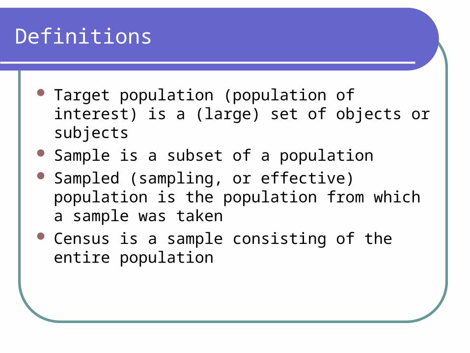
Target population (population of interest) is a (large) set of objects or subjects

Sample is a subset of a population Sampled (sampling, or effective) population is the

population from which a sample was taken Census is a sample consisting of the entire population

Target versus Sampling Populations

3

Target Population

Sampling Population

Overlap Between the Two Populations

Sample

Ideas and Issues

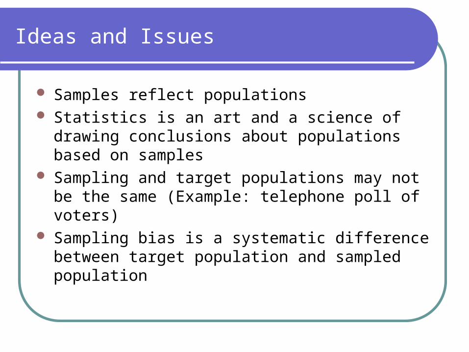
Samples reflect populations Statistics is an art and a science of drawing

conclusions about populations based on samples Sampling and target populations may not be the same

(Example: telephone poll of voters) Sampling bias is a systematic difference between

target population and sampled population

Why Not Conduct a Census?

Samples are used instead of collecting data from the entire population (that is, conducting a census) because sampling is less costly can be completed in less time may be destructive can use specialized data collection methods is the only choice when it is not possible to measure

the entire population

5

More Definitions

Observation unit, element, subject - on object or subject on which data are collected (or measurement is taken)

Sampling frame is a specification of the sampling units (e.g. a list, a map)

Sampling unit (what is sampled) may not be a population element

Sampling Units and Population Elements

7

Sampling Units Population Elements

More Definitions Continued

Overcoverage is inclusion of the units that do not belong to the target population in the sampling frame

Undercoverage is failure to include all units from the target population in the sampling frame (example: people without land telephone lines, unlisted numbers)

Selection Bias

Convenience sample: easiest to reach available units; may not reflect harder to reach or non-responding units

Judgment or subjective sample selected by a researcher

Multiplicity listings in the sampling frame (example: multiple phone numbers)

Substitution: if a person is not available, ask a family member or select another available person

Allowing sample to consist entirely of volunteers

Sampling and non-sampling errors

Sampling error results from looking at a sample instead of the entire population

Non-sampling error results from selection bias or measurement error (or other sources)

Measurement error is difference between true value and response to an item

Example: a scale to measure a latent variable Example: recall bias Example: social desirability Example: neutral option

Types of Probability Samples

Simple random sample Stratified random sample Cluster sample Systematic sample

Examples of Non-probability Samples

Convenience sample Quota sample (given numbers are selected from pre-

specified subgroups)

Simple Random Sample (SRS)

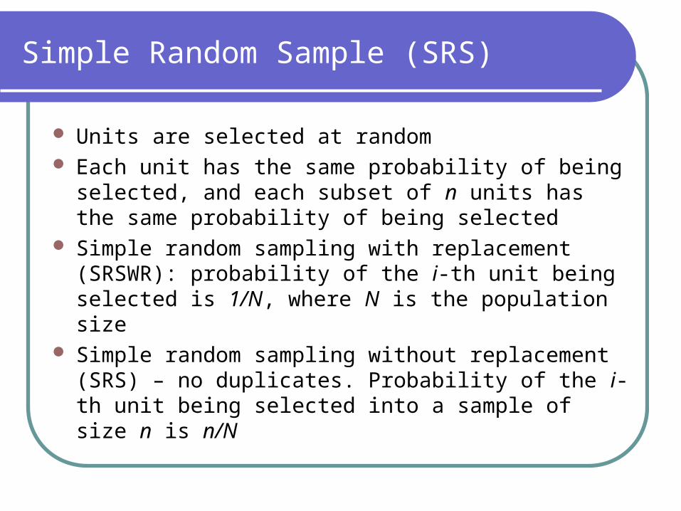
Units are selected at random Each unit has the same probability of being selected,

and each subset of n units has the same probability of being selected

Simple random sampling with replacement (SRSWR): probability of the i-th unit being selected is 1/N, where N is the population size

Simple random sampling without replacement (SRS) – no duplicates. Probability of the i-th unit being selected into a sample of size n is n/N

Stratified Random Sample

Population is divided into groups called strata SRS is selected from each stratum, and SRS’s

selected from different strata are independent Strata are often subgroups of interest such as males

or females, regions of the country, companies of certain size

Cluster Sample

Units in the population are aggregated into larger sampling units called clusters

SRS or other type of sample is selected from all clusters

Subsamples of all or some members of the cluster is selected next

Example of clusters include churches, schools, families

Example: utility poles sampling to determine “usable space”

Systematic Sample

Starting point is selected from a list of population units using a random number

That unit, and every k-th unit on the list thereafter are chosen to form the sample

Sample elements are equally spaced in the list When units in the population list are mixed (random

order), then systematic sample behaves much like SRS

When population list is not mixed, then systematic sample may not be representative of the population (e.g. student # list in increasing order)

An example of a cluster sample

Parameters and Estimators

Population parameter is a number that characterizes population

Estimator (statistic) is a function of observations in the sample used to estimate the population parameter

Example: population mean (parameter), sample mean (estimator)

n

ii

n ynn

yyyy

1

21 1...

Uy

Project 1

Instructions: project1.doc Population: rectangles of dots Population data provided

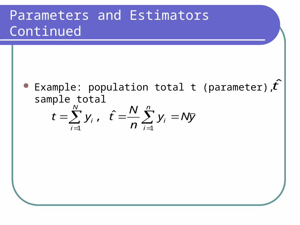
Parameters and Estimators Continued

Example: population total t (parameter), sample total t̂

n

ii

N

ii yNy

n

Ntyt

11

ˆ,

Sampling Distribution

Key issue: variability of the estimator from sample to sample

Sampling distribution is a pattern of variation of an estimator from sample to sample across all possible samples

Let t be the value of the population parameter, and be a statistic

The expected value of is the mean of the sampling distribution

The variance of is the variance of the sampling distribution

t̂t̂

t̂

Sampling Distribution

Bias:

Variance:

Mean squared error:

ttEtBias )ˆ()ˆ(

2))ˆ(ˆ()ˆ( tEtEtVar

22 ))ˆ(()ˆ()ˆ()ˆ( tBiastVarttEtMSE

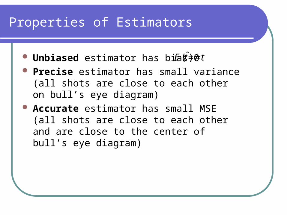
Properties of Estimators

Unbiased estimator has bias=0 Precise estimator has small variance (all shots

are close to each other on bull’s eye diagram) Accurate estimator has small MSE (all shots are

close to each other and are close to the center of bull’s eye diagram)

ttE )ˆ(

Accuracy versus Precision

High precision (low variance),

low accuracy because of bias:

MSE=Variance+Bias2

Low precision: high variance,

and therefore high MSE, so low

accuracy as well

Sample Mean

Consider finite population of N units, and introduce notation for the population mean, and the population standard deviation:

For SRS of size n,

The factor of (1-n/N) is called the finite population correction factor.

N

n

n

SyVaryyE U 1)(,)(

2

N

iUi

N

iiU yy

NSy

Ny

1

2

1

2 )(1

1,

1

samplei

iyny

1

Sample Variance

For SRS of size n,

is an unbiased estimator of the population variance.

samplei

i yyn

s 22 )(1

1

Estimator for the Variance

The variance of the sample mean is:

An unbiased estimator of the variance of the sample mean is

Standard error is

n

s

N

nyarV

2

1)(ˆ

n

S

N

nyVar

2

1)(

n

s

N

nySE

2

1)(

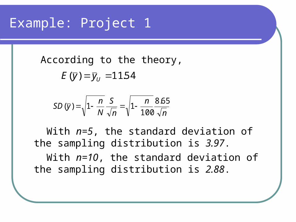
Example: Project 1

According to the theory,

With n=5, the standard deviation of the sampling distribution is 3.97.

With n=10, the standard deviation of the sampling distribution is 2.88.

54.11)( UyyE

n

n

n

S

N

nySD

65.8

10011)(

Parameter: Population Proportion

An attribute is of interest Let y=1 if attribute is present, and y=0 if attribute is

absent The population mean becomes population proportion

p The sample mean becomes the sample proportion y

total

countp ˆ

Proportion

With response values of 0 and 1

The estimators

)1(1

)(1

1,

1

22 ppN

Npy

NSpy

N

iiU

)ˆ1(ˆ1

)ˆ(1

1,

1ˆ 22 pp

n

npy

nsy

np

sampleii

sampleii

Proportion: Variance and SE

The variance of the sample proportion is:

The standard error is:

n

pp

N

nN

N

n

npp

N

N

N

n

n

SpVar

)1(

11

1)1(

11)ˆ(

2

1

)ˆ1(ˆ1)ˆ(

n

pp

N

npSE

Other Parameter: Total

Population total t:

Estimator:

Variance:

Standard error:

Note that CV is the same for sample mean and estimator of total:

N

iUi yNyt

1

yNt ˆ

n

S

N

nNtVar

22 1)ˆ(

n

s

N

nNtSE 1)ˆ(

)ˆ(/)ˆ()ˆ(ˆ tEtSEtVC

Sampling Distribution of the Sample Mean

For SRS, central limit theorem of Erdos and Renyi (1959) and Hajek (1960)

Interpretation of for finite population:

Pretend that the population of interest is part of a larger superpopulation that is in turn a pert of even larger superpopulation, and so on: series of increasing finite populations that could be as large as we wish

nN

nSNnyy U ),1,0(/1

n

Large Sample Confidence Interval

For SRS, the large sample confidence interval (CI) for the population mean is

where 100(1-α)% is the confidence level, and is 100(1-α/2)th percentile of N(0,1) distribution

Issues: a) how large does n have to be?

b) what about population standard deviation S?

n

S

N

nzy 12/

2/z

Issues

Textbook recommendation of n=30 or more may not be adequate

Consider the shape of the distribution When S is unknown, estimate it from the data with

sample standard deviation s:

Si

i yyn

s 2)(1

1

CI for the Population Mean

Using t-distribution with n-1 degrees of freedom, the CI for population mean is

where

100(1-α)% is the confidence level, and is 100(1-α/2)th percentile of t-distribution

n

s

N

nty 12/

samplei

i yyn

s )(1

1

2/t

t-CI

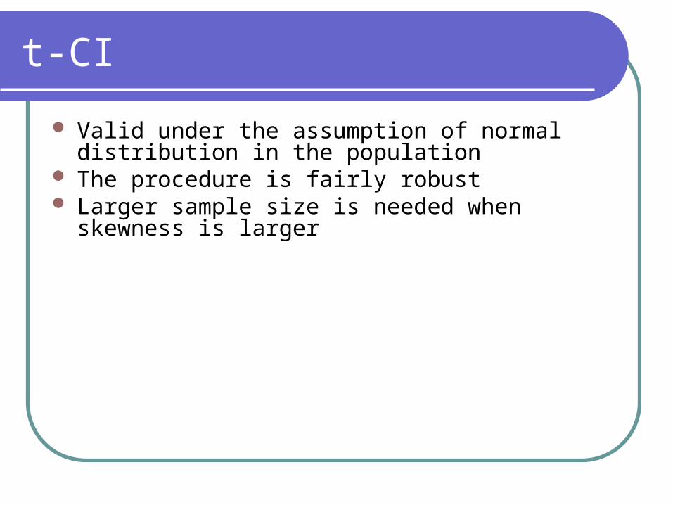
Valid under the assumption of normal distribution in the population

The procedure is fairly robust Larger sample size is needed when skewness is

larger

Sample size large enough?

Sugden (2000) extended Cochran’s rule for n needed for using normal approximation:

where is skewness in the population:

221

2

31

3

12528

)(2528

N

N

NS

yyn

N

iUi

1

31

3

2/3

1

2

1

3

33

1

)(1

1

)(1

1

)(1

1

S

yyN

yyN

yyN

S

N

iUi

N

iUi

N

iUi

Large Sample CI for Total

From the CI for the mean

get the (large sample) CI for population total:

n

s

N

nNzT

2

2/ 1ˆ

n

s

N

nty 12/

Coefficient of Variation (CV)

Coefficient of variation:

Estimated coefficient of variation:

CV is used in sample size considerations

yn

s

N

n

y

ySEyVC 1

)()(ˆ

UU yn

S

N

n

y

yVar

yE

yVaryCV 1

)(

)(

)()(

CV Example

IRS Revenue Procedures 2004-29, 2004-20, IRB 918. Disallowance of entertainment, gift, and travel expenses – use of statistical sampling methodology

Paired variable: difference between actual (audited) value of transaction and original reported value of transaction

“CV of paired variable must be 15% or less” “Sample size must be at least 100 units”

CV Example Continued

According to the IRS requirement:

122

22

22

2

2

)15.0(1

)15.0(11

)15.0(11

)15.0(1

1

s

y

Nn

s

y

Nn

s

y

Nn

y

s

nN

n

Sample Size via Relative Precision

In general, suppose we require that the margin of error of the CI does not exceed .

This is equivalent toUyr

.)(

,)(

)(

)()(

2/

2/

2/

z

ryCV

z

r

yE

yVar

yrEyryVarz U

Sample Size Based on Relative Precision

If we want the margin of error of the confidence interval not to exceed then

Uyr

NSz

yr

Szn

SzyNr

SNzn

yrn

S

N

nz

U

U

U

222/2

222/

222/

22

222/

2/

)(

,

,1

Sample Size Based on Absolute Precision

Find the sample size so that the margin of error of the CI does not exceed specified number e:

NzS

e

zSn

zSNe

zNSn

en

S

N

nz

22/

22

22/

2

22/

22

22/

2

2/ ,1

Sample Size Continued

The last formula is convenient (discard a term with N if N is large):

For SRSWR:

Connection with SRS:

NzS

e

zSn 2

2/2

2

22/

2

2

22/

2

0 e

zSn

N

nnn0

0

1

Example Calculation

Example (along the lines of IRS audit):

Suppose the population consists of N=7,000 receipts. A sample has to be drawn so that the half length of the CI for mean difference (true actual amount – reported amount) does not exceed 0.2 standard deviation units: e/S≤0.2. Then

66.95014.1

97

000,797

1

97

1

,04.9696.12.0

1

0

0

22

22/2

2

0

N

nn

n

ze

Sn

Example Calculation Continued

The IRS requirement of CV≤0.15 in relative precision language means that r=0.15*1.96=0.294.

We need estimates for the mean and standard deviation of the differences (for example, from past year). Suppose that S=$200, and

37.173952.2136.864

664,153

000,720096.1

)100294.0(

20096.122

2

22

n

100$Uy

Example Calculation Continued

Assume (based on past year) that S=$200, and

150$Uy

13.78952.2181.1944

664,153

000,720096.1

)150294.0(

20096.122

2

22

n

Sampling Weights

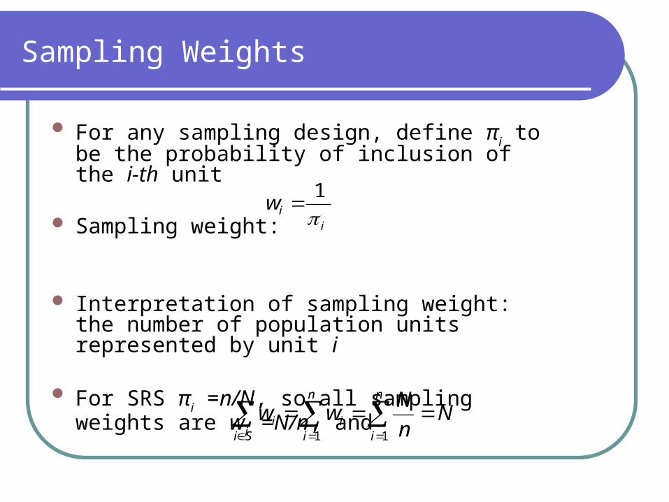
For any sampling design, define πi to be the probability of inclusion of the i-th unit

Sampling weight:

Interpretation of sampling weight: the number of population units represented by unit i

For SRS πi =n/N, so all sampling weights are wi =N/n, and

iiw

1

Nn

Nww

n

i

n

ii

Sii

11

Sampling Weights - SRS

For the estimator of population total from SRS:

For the sample mean:

Self-weighting sample: a sample in which every unit has the same weight

Sii

iSi

i

w

yw

N

ty

ˆ

Si

iiiSi

ywyn

Nt̂

Considerations for Using SRS

Consider if you need a survey or a controlled experiment

Is the sampling frame available? Is there an additional information for use in study

design? Is the focus of the study on one variable or

relationships among multiple variables?

Stratified Sampling

SRS may not contain units from some subgroups:

when sampling 10 people from a population of 60 males and 40 females, the entire SRS can consist of females

Stratified sampling can ensure that both males and females are represented in the sample

Stratified sampling can ensure given precision in each subgroup

Stratified sampling often results in higher precision (lower variance of estimates)

Stratified Sampling Continued

Strata are subgroups or subpopulations of the entire population

Notation H for the number of strata The sizes of the strata are known. Stratum h has the

size Nh, and NNNN H ...21

Stratified Sampling Strategy

Take an SRS from each stratum Selection probability may be the same across strata,

or may not be the same If variance in one strata is larger, more data could be

sampled from that strata Let the sample from stratum h have the size nh so that

the total sample size is

Hnnnn ...21

Notation: Stratum Population Quantities

Value j in stratum h is yhj

Total in stratum h:

Mean in stratum h:

Variance in stratum h:

hN

jhjh yt

1

hN

j h

hhj

hhU N

ty

Ny

1

1

hN

j h

hUhjh N

yyS

1

22

1

)(

Notation: Overall Population Quantities

Population total:

Overall mean:

hN

jhj

H

hh

H

h

ytt111

N

y

N

ty

hN

jhj

H

hU

11

Notation: Stratum Estimators

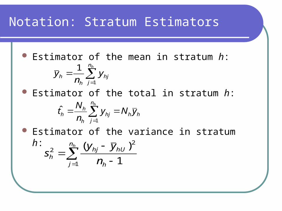
Estimator of the mean in stratum h:

Estimator of the total in stratum h:

Estimator of the variance in stratum h:

hh

n

jhj

h

hh yNy

n

Nt

h

1

ˆ

hn

jhj

hh yn

y1

1

hn

j h

hUhjh n

yys

1

22

1

)(

Notation: Overall Estimators

Estimator of the population total:

Estimator of the overall mean:

H

hhhh

H

hstr yNtt

11

ˆˆ

h

H

h

hstrstr y

N

N

N

ty

1

ˆ

Estimators Continued

The estimator of overall mean is a weighted average of stratum averages

Weight of stratum h mean is Nh / N

Relative sizes of strata must be known Since sampling is done independently across

strata, properties of overall estimators follow from properties of SRS estimators

Properties of Estimators

Unbiasedness:

Variance of the estimator of total:

Standard error of the estimator of total:

H

h h

h

h

hhh

H

hstr n

S

N

nNtVartVar

1

22

1

1)ˆ()ˆ(

H

hUhhU

H

h

hh

H

h

hstr yt

Ny

N

NyE

N

NyE

111

1)()(

H

h h

h

h

hhstr n

s

N

nNtSE

1

22 1)ˆ(

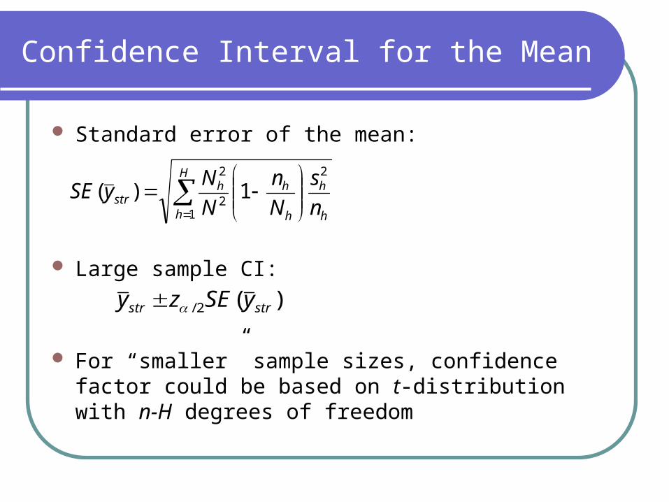
Confidence Interval for the Mean

Standard error of the mean:

Large sample CI:

For “smaller” sample sizes, confidence factor could be based on t-distribution with n-H degrees of freedom

)(2/ strstr ySEzy

H

h h

h

h

hhstr n

s

N

n

N

NySE

1

2

2

2

1)(

Stratified Sampling: Allocation Types

Proportional allocation:

Proportional allocation results in a sample resembling SRS for large n

Neyman allocation (minimizes variance):

Neyman allocation is used if costs of collecting data in each stratum are the same

nSN

SNn H

iii

hhNeymanh

1

,

nN

Nn h

alproportionh ,

Project 2: Stratified Sampling

Project 2 – select a sample of counties stratified by region

In the population of N=3078 counties H=4 regions (strata) are identified:

Northeast N1=220 (7.15%)

North CentralN2=1054 (34.24%)

South N3=1382 (44.90%)

West N4=422 (13.71%)

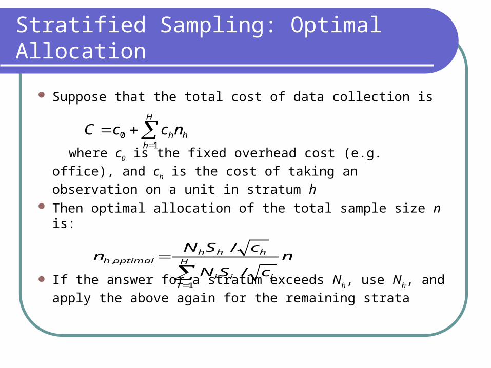
Stratified Sampling: Optimal Allocation

Suppose that the total cost of data collection is

where c0 is the fixed overhead cost (e.g. office), and ch is

the cost of taking an observation on a unit in stratum h Then optimal allocation of the total sample size n is:

If the answer for a stratum exceeds Nh, use Nh, and

apply the above again for the remaining strata

ncSN

cSNn H

iiii

hhhoptimalh

1

,

/

/

H

hhhnccC

10

Allocation in Stratified Sampling

Larger sample size within stratum is needed when- Stratum is larger- Variance in the stratum is larger- Sampling within stratum has low cost

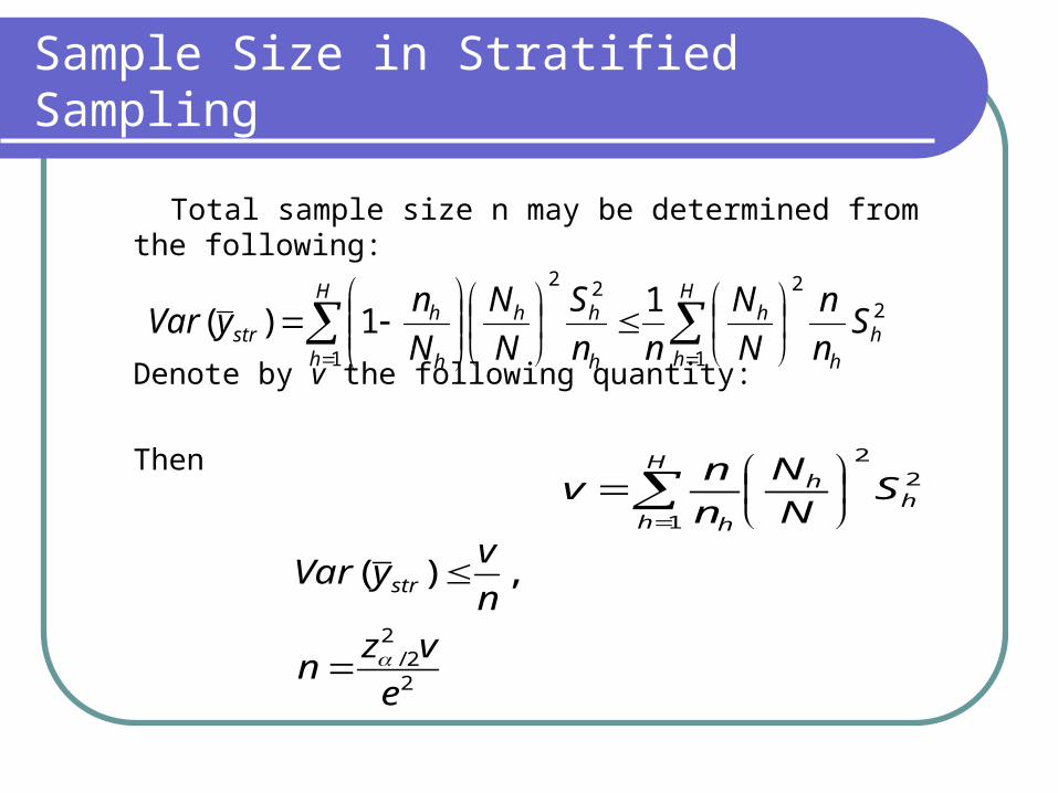
Sample Size in Stratified Sampling

Total sample size n may be determined from the following:

Denote by v the following quantity:

Then

2

1

222

1

11)( h

h

H

h

h

h

hH

h

h

h

hstr S

n

n

N

N

nn

S

N

N

N

nyVar

22

1h

hH

h h

SN

N

n

nv

2

22/

,)(

e

vzn

n

vyVar str

Stratified Sampling for Proportions

As we saw earlier, proportion is a mean of a sample of 0’s and 1’s, so in stratum h

Overall:

)ˆ1(ˆ1

,ˆ 2hh

h

hh

hh pp

n

ns

n

hstratumincountp

H

hhhstrh

H

h

hstr pNtp

N

Np

11

ˆˆ,ˆˆ

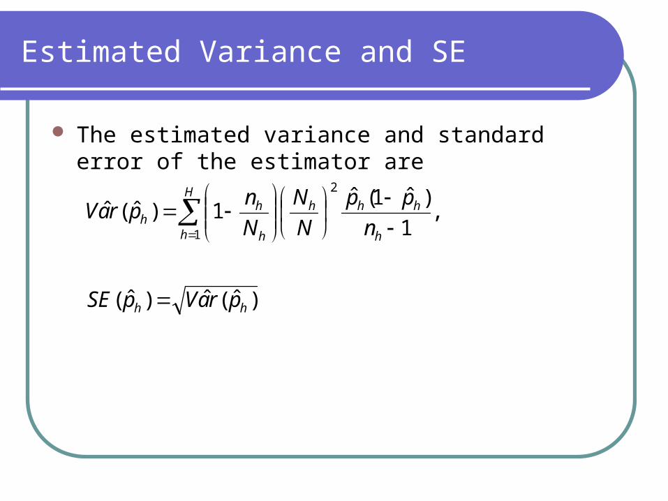
Estimated Variance and SE

The estimated variance and standard error of the estimator are

)ˆ(ˆ)ˆ(

,1

)ˆ1(ˆ1)ˆ(ˆ

1

2

hh

H

h h

hhh

h

hh

praVpSE

n

pp

N

N

N

npraV

An Application

Cohort of patients is followed up over time, for example, breast cancer patients are enrolled at the time of diagnosis

After surgery, an extensive study of tumor and nodes pathology is planned, but it is very expensive

Problem: select a subcohort, but the selection may not be handled by running a software

An Application Continued

Example: potentially most interesting cases to be studied in detail include women in their 30’s, 40’s, and those with stage III or IV

Consider 2 categorical variables: age (30-39, 40-49, or ≥50), and stage of cancer (I or II versus III or IV)

These variables define 6 strata

Hypothetical Counts

Stratum Cohort count

Sub-cohort count

Selection prob.

Weight

30-39, early stage 50 40 .8 1.25

40-49, early stage 200 150 .75 1.33

50+, early stage 250 50 .2 5

30-39, late stage 30 30 1 1

40-49, late stage 100 100 1 1

50+, late stage 150 140 .93 1.07

Data Analysis with SURVEY Procedures

Example uses of SURVEY procedures Weights can be included in the file (e.g. if SURVEYSELECT

procedure was used), or need to be defined as in the previous example

Example code for regression:

proc surveyreg data=samplestrataN total=region2;

strata region /list;

weight SamplingWeight;

model acres92=acres87;

run;

 

SURVEY Procedures Continued

Example code for cross-tabulation (with categorical variables I92, I87):

proc surveyfreq data=samplestrataN total=region2;

strata region /list;

weight SamplingWeight;

tables l92*l87 / chisq;

run;

 

SURVEY Procedures Continued

Example code for logistic regression:

proc surveylogistic data=samplestrataN total=region2;

strata region /list;

weight SamplingWeight;

class l92;

model l92(event='1')=acres87;

run;

 

References

1. Lohr S. (2009) Sampling: Design and Analysis. Brooks/Cole, Boston, MA.

2. SAS 9.2 software © 2009, SAS Institute Inc.

3. Hajek J. (1964) Asymptotic theory of rejection sampling with varying probabilities from a finite population. Annals of Mathematical Statistics, 35, 1491-1523.

4. Erdos P and Renyi A. (1959) On the central limit theorem for samples from a finite population. Publ. Natl. Hungar. Acad. Sci. 4, 49-61.

5. Rao JNK, Scott AJ. (1981) The analysis of categorical data from complex sample surveys: Chi-squared tests for goodness of fit and independence in two-way tables. J Royal Stat. Soc. Ser. B, 24, 482-491

References Continued

6. Rao JNK, Scott AJ and Benhin E (2003) Undoing complex survey data structures: Some theory and applications of inverse sampling. Survey Methodology, 29(2), 107-121.

7. Krewski D and Rao JNK (1981) Inference from stratified samples: Properties of the linearization, jackknife, and balanced repeated replication methods. The Annals of Statistics, 9, 1010-1019.

8. Sugden RA, Smith TMF and Jones RP. (2000) Cochran’s rule for simple random sampling. J. Royal Stat. Soc. Ser. B, 62 787-793.