Introduction to Robotics Module: Trajectory generation · PDF fileIntroduction to Robotics:...
50
Introduction to Robotics: Module Trajectory generation and robot programming FH Darmstadt, summer term 2000 E:\Robot_Erw\Publications\LectureRobotics.doc 1/50 Introduction to Robotics Module: Trajectory generation and robot programming (summer term 2000) Recommended literature Text Books • Craig,J.J.: Introduction to Robotics. Addison-Wesley, 2nd. Ed, 1989 (3 rd edition will be available 2000 ?) • Craig,J.: Adaptive Control of Mechanical Manipulators. Addison-Wesley, Reading(Mass.), 1988 • R.P. Paul: Robot Manipulators, MIT Press 1981 Journals • Transactions on Robotics and Automation, IEEE • IEEE Conference on Robotics and Automation Acknowledgement This handout has been partially derived from the lecture notes from Wolfgang Weber teaching robotics at the Fachhochschule Darmstadt, Germany and the above mentioned textbooks from J.J. Craig and R.P. Paul. Revisions Revision Date Author History 0.9 12-Mar-99 Th. Horsch 1 st draft 1.0 20.2.2000 Th. Horsch 1 st release
Transcript of Introduction to Robotics Module: Trajectory generation · PDF fileIntroduction to Robotics:...
Introduction to Robotics: Module Trajectory generation and robot programmingFH Darmstadt, summer term 2000
E:\Robot_Erw\Publications\LectureRobotics.doc 1/50
Introduction to Robotics
Module:Trajectory generation and robot programming
(summer term 2000)
Recommended literature
Text Books
• Craig,J.J.: Introduction to Robotics. Addison-Wesley, 2nd. Ed, 1989 (3rd edition will beavailable 2000 ?)
• Craig,J.: Adaptive Control of Mechanical Manipulators. Addison-Wesley, Reading(Mass.),1988
• R.P. Paul: Robot Manipulators, MIT Press 1981
Journals
• Transactions on Robotics and Automation, IEEE
• IEEE Conference on Robotics and Automation
Acknowledgement
This handout has been partially derived from the lecture notes from Wolfgang Weberteaching robotics at the Fachhochschule Darmstadt, Germany and the above mentionedtextbooks from J.J. Craig and R.P. Paul.
Revisions
Revision Date Author History0.9 12-Mar-99 Th. Horsch 1st draft1.0 20.2.2000 Th. Horsch 1st release
Introduction to Robotics: Module Trajectory generation and robot programmingFH Darmstadt, summer term 2000
E:\Robot_Erw\Publications\LectureRobotics.doc 2/50
CONTENT
1. MOTIVATION ........................................................................................................................ 3
1.1. WHY STUDY ROBOTICS ...................................................................................................... 31.2. TERMINOLOGY.................................................................................................................. 31.3. TYPES OF ROBOT MOTION.................................................................................................. 6
2. SPATIAL DESCRIPTIONS AND TRANSFORMATIONS ....................................................... 8
2.1. DESCRIPTIONS: POSITIONS, ORIENTATIONS AND FRAMES ...................................................... 82.2. CONSIDERATIONS ........................................................................................................... 142.3. ORIENTATION DEFINED BY EULER-ANGLES ........................................................................ 15
3. ROBOT KINEMATICS......................................................................................................... 19
3.1. LINK CONNECTION DESCRIPTION BY DENAVIT-HARTENBERG NOTATION................................. 193.2. FORWARD KINEMATICS .................................................................................................... 263.3. INVERSE KINEMATICS ...................................................................................................... 27
4. TRAJECTORY GENERATION ............................................................................................ 34
4.1. TRAJECTORY GENERATION IN JOINT SPACE (PTP MOTIONS) ................................................ 344.2. ASYNCHRONE PTP AND SYNCHRONE PTP ....................................................................... 384.3. TRAJECTORY GENERATION IN CARTESIAN SPACE ................................................................ 38
4.3.1. Linear Interpolation................................................................................................... 394.3.2. Circular interpolation................................................................................................. 434.3.3. Corner smoothing..................................................................................................... 44
4.4. SPLINE INTERPOLATION BASED ON BÉZIER CURVES ............................................................ 45
5. ROBOT PROGRAMMING LANGUAGES ............................................................................ 49
5.1. REQUIREMENTS OF A ROBOT PROGRAMMING LANGUAGE ..................................................... 50
Introduction to Robotics: Module Trajectory generation and robot programmingFH Darmstadt, summer term 2000
E:\Robot_Erw\Publications\LectureRobotics.doc 3/50
1. Motivation
1.1. Why study robotics
Robots are mainly used for
• Automation of industrial tasks• Spot welding• Arc welding• Machine transfer and machine tending• Pick and Place• Clueing and sealing• Deburring• Assembly/Disassembly
• Testbed for Artificial Intelligence (AI)
Robotics is an interdisciplinary subject requiring
Mechanical Engineering (addressed in module Components of a robotarm)
Electrical/Electronic Engineering (addressed in module Control of a robot arm)Computer Science/Mathematics (addressed in this module)
It is worth noting that many problems in computer graphics animation are related torobotics problems (much of the material in this course is relevant to animation).
1.2. Terminology
We begin with some robot terminology.
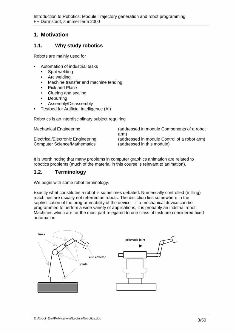
Exactly what constitutes a robot is sometimes debated. Numerically controlled (milling)machines are usually not referred as robots. The distiction lies somewhere in thesophistication of the programmability of the device – if a mechanical device can beprogrammed to perfom a wide variety of applications, it is probably an indstrial robot.Machines which are for the most part relegated to one class of task are considered fixedautomation.
prismatic joint
links
end effector
joints
Introduction to Robotics: Module Trajectory generation and robot programmingFH Darmstadt, summer term 2000
E:\Robot_Erw\Publications\LectureRobotics.doc 4/50
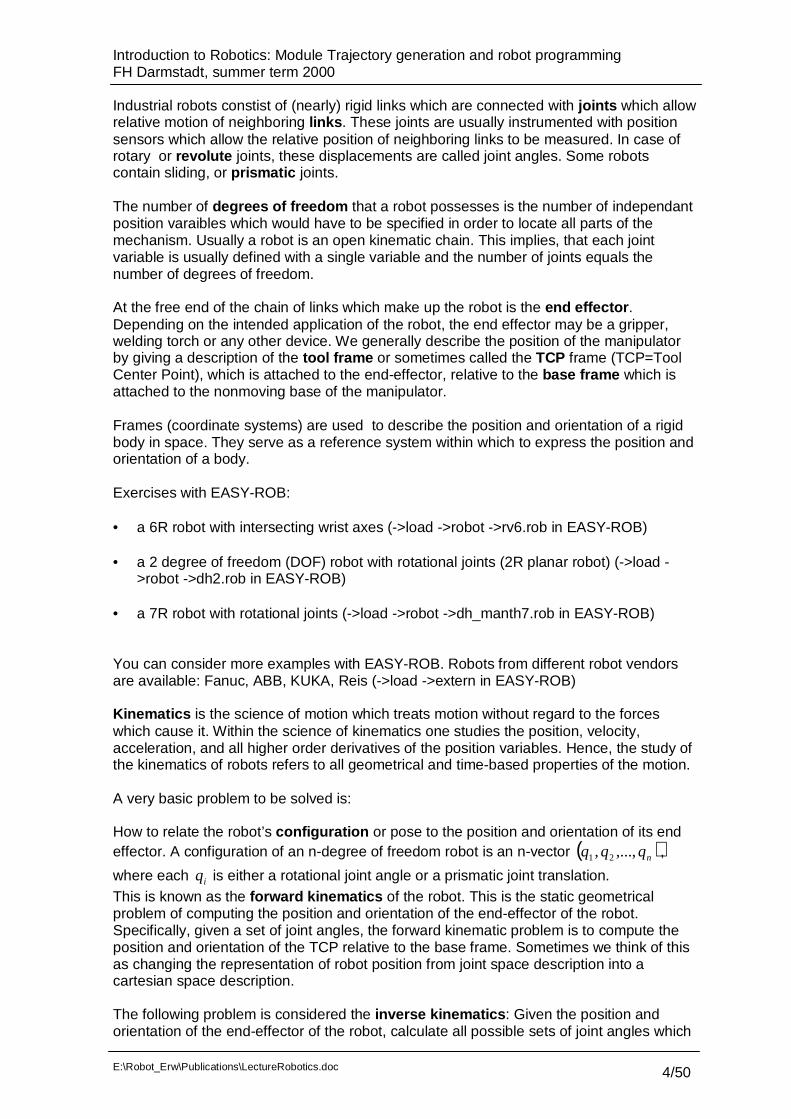
Industrial robots constist of (nearly) rigid links which are connected with joints which allowrelative motion of neighboring links. These joints are usually instrumented with positionsensors which allow the relative position of neighboring links to be measured. In case ofrotary or revolute joints, these displacements are called joint angles. Some robotscontain sliding, or prismatic joints.
The number of degrees of freedom that a robot possesses is the number of independantposition varaibles which would have to be specified in order to locate all parts of themechanism. Usually a robot is an open kinematic chain. This implies, that each jointvariable is usually defined with a single variable and the number of joints equals thenumber of degrees of freedom.
At the free end of the chain of links which make up the robot is the end effector.Depending on the intended application of the robot, the end effector may be a gripper,welding torch or any other device. We generally describe the position of the manipulatorby giving a description of the tool frame or sometimes called the TCP frame (TCP=ToolCenter Point), which is attached to the end-effector, relative to the base frame which isattached to the nonmoving base of the manipulator.
Frames (coordinate systems) are used to describe the position and orientation of a rigidbody in space. They serve as a reference system within which to express the position andorientation of a body.
Exercises with EASY-ROB:
• a 6R robot with intersecting wrist axes (->load ->robot ->rv6.rob in EASY-ROB)
• a 2 degree of freedom (DOF) robot with rotational joints (2R planar robot) (->load ->robot ->dh2.rob in EASY-ROB)
• a 7R robot with rotational joints (->load ->robot ->dh_manth7.rob in EASY-ROB)
You can consider more examples with EASY-ROB. Robots from different robot vendorsare available: Fanuc, ABB, KUKA, Reis (->load ->extern in EASY-ROB)
Kinematics is the science of motion which treats motion without regard to the forceswhich cause it. Within the science of kinematics one studies the position, velocity,acceleration, and all higher order derivatives of the position variables. Hence, the study ofthe kinematics of robots refers to all geometrical and time-based properties of the motion.
A very basic problem to be solved is:
How to relate the robot’s configuration or pose to the position and orientation of its endeffector. A configuration of an n-degree of freedom robot is an n-vector ( )nqqq ,...,, 21 ,
where each iq is either a rotational joint angle or a prismatic joint translation.This is known as the forward kinematics of the robot. This is the static geometricalproblem of computing the position and orientation of the end-effector of the robot.Specifically, given a set of joint angles, the forward kinematic problem is to compute theposition and orientation of the TCP relative to the base frame. Sometimes we think of thisas changing the representation of robot position from joint space description into acartesian space description.
The following problem is considered the inverse kinematics: Given the position andorientation of the end-effector of the robot, calculate all possible sets of joint angles which

Introduction to Robotics: Module Trajectory generation and robot programmingFH Darmstadt, summer term 2000
E:\Robot_Erw\Publications\LectureRobotics.doc 5/50
could be used to attain the this given position and orientation. The inverse kinematics isnot as simple as the forward kinematics. Because the kinematic equations are nonlinear,their solution is not always easy or even possible in a closed form. The existence of akinematic solution defines the workspace of a given robot. The lack of a solution meansthat the robot cannot attain the desired position and orientation because it lies outside therobot’s workspace.
In addition to dealing with static positioning problems, we may wish to analyse robots inmotion. Often in performing velocity analysis of a mechanism it is convenient to define amatrix quantity called the jacobian of the robot. The jacobian specifies a mapping fromvelocities in joint space to velocities in cartesian space. The nature of this mappingchanges as the configuration of the robot varies. At certain points, called singularities, thismapping is not invertible. An understanding of this phenomenon is important to designersand users of robots.
A common way of causing a robot to move from A to B in a smooth, controlled fashion isto cause each joint to move as specified by a smooth function of time. Commonly, eachjoint starts and ends ist motion at the same time, so that the robot motion appearscoordinated. Exactly how to compute these motion functions is the problem of trajectorygeneration.
A robot programming language serves as an interface between the human user and theindustrial robot. Central questions arise such as:How are motions through space described easily by a programmer ?How are multiple robots programmed so that they can work in parallel ?How are sensor-based actions described in a language ?
The sophistication of the user interface is becoming extremely important as robots andother programmable devices are applied to more and more demanding industrialapplications.
An off-line programming system is a robot programming environment which has beensufficiently extended, generally by means of computer graphics, so that the developmentof robot programs can take place without access to the robot itself. A common argumentraised in the favor is that an off-line programming system will not cause productionequipment (i.e. the robot) to be tied up when it needs to be reprogrammed; hence,automated factories can stay in production mode a greater percentage of time.
A robot constists of three main systems:
• Programming system:
A robot user needs to „teach“ the robot the specific task which is to be performed. Thiscan be done with the so called teach in method. The programmer uses the teach box ofthe robot control and drives the robot to the diesired positions and stores them and othervalues like travel speed, corner smoothing parameters, process parameters, etc. For theprogramming period which can take a significant time for complex tasks the production isidle. Another possibility is the use of Off-line programming systems mentioned before.
• Robot control:

Introduction to Robotics: Module Trajectory generation and robot programmingFH Darmstadt, summer term 2000
E:\Robot_Erw\Publications\LectureRobotics.doc 6/50
The robot control interprets the robot’s application program and generates a series of jointvalues and joint velocities (and sometimes accellerations) in an appropriate way for thefeedback control. Today mainly an independant joint control approach is taken, but moreand more sophisticated control approaches, like adaptive control, nonlinear control, etcare involved in robotics. The following figure shows a possible control structure.
Figure 1-1: structure of a robot control
• Robot mechanics:
The robot mechanics will transform the joint torques applied by the servo drives into anappropriate motion. Nowadays AC motors are used to drive the axis.Resolvers serve as a position sensor and are normally located on the shaft of theactuator. Resolvers are devices which output two analog signals – one is the sine of theshaft angle and the other the cosine. The shaft angle is determined from the relativemagnitude of the two signals.
1.3. Types of robot motion
PTP(Point to Point)-motion
A motion which specifies the configuration of the robot at the start and the end point. Themotion between these points is not determined in the sense that the TCP follows adesired (cartesian) path. This motion type is mainly relevant for pick and place type tasks,where the position and orientation along the path is not important. Since this motion isvery hard to predict in cartesian space, the programmer has to be careful regardingcollisions between the robot and ist environment. On the other hand this motion is easy(and fast) in calculation, because no transformation of inverse kinematics needs to becomputed.
Figure 1-1 describes two examples:
externalcontrol
coordinatetransformation
internalcontrol(joint-control)
measuredjoint values
world coordinates(desired) joint values
(desired)
sensor signals

Introduction to Robotics: Module Trajectory generation and robot programmingFH Darmstadt, summer term 2000
E:\Robot_Erw\Publications\LectureRobotics.doc 7/50
A
B
y
x x
y
°°
Bsp.: Tan
r an
ns
spo
orr
pick and placedrilling table
Figure 1-1: PTP-motions in world coordinate system, left: path bewteen two drilling holes,right: robot end-effector and three configurations for pick & place
Applications for PTP motions are spot welding, handling, pick and place, (partly) machinehandling and machine transfer
CP (Continuous Path) motion
A motion type which specifies the whole path regarding position and orientation of theTCP. That means that the motions of each axes are mutually depending. These motionsare more computationally expensive to execute at run time compared to PTP motions,since inverse kinematics must be solved for each time step (usually around 10milliseconds in todays robot controller). Possible cartesian motion types include linearinterpolation (specified by start and end point) and circular interpolation (specified by startpoint, via point and end point).Figure 1-2 describes two examples
y
x x
y via point
Figure 1-2: example for interpolated motions between programmed positions, left: asequence consisting of 5 linear motion, right: linear – circular – linear motion
Applications for CP motions are arc welding, deburring, clueing, etc.
Introduction to Robotics: Module Trajectory generation and robot programmingFH Darmstadt, summer term 2000
E:\Robot_Erw\Publications\LectureRobotics.doc 8/50
2. Spatial descriptions and transformationsThe following section summarizes the main mathematical methods in order to describepositions and orientations with respect to a particular coordinate system.
2.1. Descriptions: positions, orientations and frames
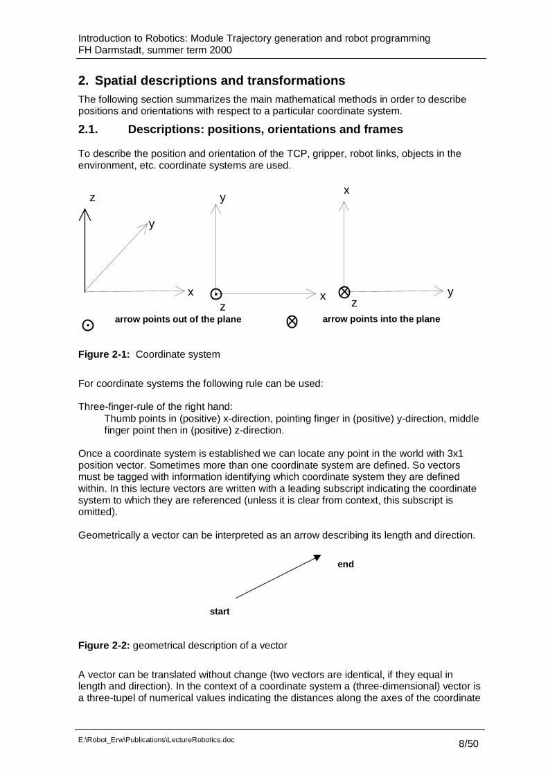
To describe the position and orientation of the TCP, gripper, robot links, objects in theenvironment, etc. coordinate systems are used.
yz
x x
x
y
yz
z arrow points out of the plane arrow points into the plane
Figure 2-1: Coordinate system
For coordinate systems the following rule can be used:
Three-finger-rule of the right hand:Thumb points in (positive) x-direction, pointing finger in (positive) y-direction, middlefinger point then in (positive) z-direction.
Once a coordinate system is established we can locate any point in the world with 3x1position vector. Sometimes more than one coordinate system are defined. So vectorsmust be tagged with information identifying which coordinate system they are definedwithin. In this lecture vectors are written with a leading subscript indicating the coordinatesystem to which they are referenced (unless it is clear from context, this subscript isomitted).
Geometrically a vector can be interpreted as an arrow describing its length and direction.
Figure 2-2: geometrical description of a vector
A vector can be translated without change (two vectors are identical, if they equal inlength and direction). In the context of a coordinate system a (three-dimensional) vector isa three-tupel of numerical values indicating the distances along the axes of the coordinate
start
end

Introduction to Robotics: Module Trajectory generation and robot programmingFH Darmstadt, summer term 2000
E:\Robot_Erw\Publications\LectureRobotics.doc 9/50
system. Each of these distances along an axis can be thought of as a result of projectingthe vector onto the corresponding axis.
=
z
y
x
v
v
v
v z x
y
v
vx
yv
Figure 2-3: description of a vector in a coordinate system
modulus (length) of a vectors: v v v vx y z= + +2 2 2
(2.1)
(unit) direction of a vector:
==
v/v
v/v
v/v
vv
e
z
y
x
v (2.2)
addition of vectors:
+++
=+=
z2z1
y2y1
x2x1
213
vv
vv
vv
vvv
v12
3
v
v(2.3)
subtraction of vectors:
−−−
=−
z2z1
y2y1
x2x1
21
vv
vv
vv
vv v1
2v2
v v1 --
(2.4)
cross product of two vectors: v v v3 1 2= ×

Introduction to Robotics: Module Trajectory generation and robot programmingFH Darmstadt, summer term 2000
E:\Robot_Erw\Publications\LectureRobotics.doc 10/50
⋅−⋅⋅−⋅⋅−⋅
=
=
x2y1y2x1
z2x1x2z1
y2z1z2y1
z3
y3
x3
3
vvvv
vvvv
vvvv
v
v
v
v (2.5)
v3 is orthogonal to the plane, generated by v1 and v2. The three-finger-rule derives thedirection of v3 (see Figure 2-4).
3v
v1
2v
..
Figure 2-4: cross product
Dot product of two vectors:
The dot product of two vectors is defined by (2.6). The result is a scalar value which isrelated to the opening angle between the vectors. If one of the vectors is a unit vector (avector with unit length) the result is the length of projection onto the unit vector. (seeFigure 2-5).
a b a b⋅ = ⋅ ⋅cosϕ , zzyyxx babababa ⋅+⋅+⋅=⋅ (2.6)
Figure 2-5: dot product of two vectors
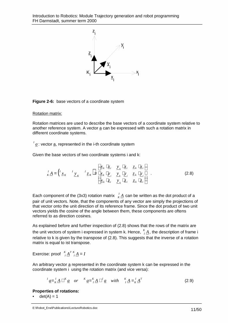
Base vectors xi , yi , zi of the coordinate system Ki . A cartesian coordinate system is fully
described by ist base vectors xi, yi, zi, which are orthogonal to each other (Figure 2-6).
)(1,
1
0
0
,
0
1
0
,
0
0
1
vectorsunitzyxzyx iiiiii −===
=
=
= (2.7)
ϕ
Introduction to Robotics: Module Trajectory generation and robot programmingFH Darmstadt, summer term 2000
E:\Robot_Erw\Publications\LectureRobotics.doc 11/50
i
z
xi
yi
i
xi
yi
zi
K
Figure 2-6: base vectors of a coordinate system
Rotation matrix:
Rotation matrices are used to describe the base vectors of a coordinate system relative toanother reference system. A vector a can be expressed with such a rotation matrix indifferent coordinate systems.
aI : vector a, represented in the i-th coordinate system
Given the base vectors of two coordinate systems i and k:
( )
⋅⋅⋅⋅⋅⋅⋅⋅⋅
==
ikikik
ikikik
ikikik
KI
K
IK
IIK
zzzyzx
yzyyyx
xzxyxx
zyxA . (2.8)
Each component of the (3x3) rotation matrix AIK can be written as the dot product of a
pair of unit vectors. Note, that the components of any vector are simply the projections ofthat vector onto the unit direction of its reference frame. Since the dot product of two unitvectors yields the cosine of the angle between them, these components are oftensreferred to as direction cosines.
As explained before and further inspection of (2.8) shows that the rows of the matrix are
the unit vectors of system i expressed in system k. Hence, AKI , the description of frame i
relative to k is given by the transpose of (2.8). This suggests that the inverse of a rotationmatrix is equal to ist transpose.
Exercise: proof IAA KI
TKI =
An arbitrary vector a represented in the coordinate system k can be expressed in thecoordinate system i using the rotation matrix (and vice versa):
TIK
KI
IKI
KKIK
I AAwithaAaoraAa =⋅=⋅= (2.9)
Properties of rotations:• det(A) = 1

Introduction to Robotics: Module Trajectory generation and robot programmingFH Darmstadt, summer term 2000
E:\Robot_Erw\Publications\LectureRobotics.doc 12/50
• columns are mutually orthogonal• possible to describe rotations with fewer than 9 numbers• result from linear algebra: Cayley’s formula for orthogonal matrices
( ) ( )
=−=+−= −
0
0
0
, symmetric scew is S ,31
3
xy
xz
yz
T
s-s
-ss
s-s
S)S(SSISIR
• three parameters to describe rotation
• same result by investigation of R• six constraints and nine matrix elements
0
1
===
===
zxzyyx
zyxTTT
• rotations do not generally commute: 1221 RRRR ≠
Exercise:
Calculate )2
()2
(ππ
ZX RotRot and )2
()2
(ππ
XZ RotRot and solve both compound
transformations geometrically by drawing a frame diagram.
Homogeneous coordinates (frames)4x4 homogeneous transforms are used to cast the rotation and translation of a generaltransform into a single matrix form. In other fields of study it can be used to computeperspective and scaling operations. Hence, they describe the spatial relationship betweentwo coordinate systems (see Figure 2-7).
⋅
=
1101
apAa K
T
IIK
I
• 1 added as the last element of the 4x1 vector• row (0 0 0 1) is added as last row of 4x4 matrix
Figure 2-7: spatial relationship between two coordinate systems
pzyx IK
I
K
IK
I ,,,
pkx
ky
kz
iz
iy
ixKI
KK

Introduction to Robotics: Module Trajectory generation and robot programmingFH Darmstadt, summer term 2000
E:\Robot_Erw\Publications\LectureRobotics.doc 13/50
The homogeneous transform DIK can be viewed as the representation of the vectors xk,
yk, zk, p in the i-th coordinate system:
=
1000K
IK
I
K
IK
II
K
pzyxD (2.10)
Homogeneous transforms of several coordinate systems (compound transformations):
Combining two transformations is performed by multiplication of two homogenoustransforms (see Figure 2-8):
=⋅= +++++
+++1000
22221212
I
II
I
I
II
III
II
II
pzyxDDD (2.11)
K
K
i+1
i+2
i+1
i+2
xy
z
x
y
z
i+2i+2
i+1
i+1
pi+1
K
i
x
y
z
i
i
i
p
pi
i+2
Figure 2-8: Compound transformations
Exercise:
• Describe rotational and translational part of DII 2+ in terms of the rotational and
translational parts of DII 1+ and DI
I12
++ .
• Invert a homogenous transform
=
10T
pRD
Interpretations:
• A homogeneous transform is a description of a frame. DIK describes the frame K
relative to the frame I. Specifically, the columns of RIK are unit vectors defining the
principal axes of frame K and p locates the position of the origin of K relativ to frame I.

Introduction to Robotics: Module Trajectory generation and robot programmingFH Darmstadt, summer term 2000
E:\Robot_Erw\Publications\LectureRobotics.doc 14/50
• A homogeneous transform is a mapping. DIK maps PP IK �
.
2.2. Considerations
Consideration of robots only with open kinematic chain
Example:
BaseBase
Endeffector
JointsBase
Links
Figure 2-1: possible design of robots and their schematic sketch
Figure 2-2: Description of the position and orientation of the tool center point (TCP) withrespect to the base (world) frame K0
o
n0z
0y
0x
p
K0
TCP

Introduction to Robotics: Module Trajectory generation and robot programmingFH Darmstadt, summer term 2000
E:\Robot_Erw\Publications\LectureRobotics.doc 15/50
Attached to the TCP is the tool frame described by
Translation p with respect to K0 (Position)n, o, a with respect to K0 (Orientation)
Rotation matrix representing the orientation:
( )aon 000 ,, : normal, orthogonal, approach
homogeneous transformation integrating position and orientation with respect to baseframeK0:
==
1000
00000 paonDT N (2.12)
Index n denotes the degree of freedom of the robot
2.3. Orientation defined by Euler-Angles
Avoid redundant information by introduction of angles
translation p with respect to K0 (Position)three angles a, b, c (Orientierung)
Fixed angles: rotation takes place around fixed frameEuler angles: rotation takes place around moving frame
Definition: X-Y-Z fixed angles
a: rotation around the z0-axisb: rotation around the y0-axisc: rotation around the x0-axis
Each of the three rotations takes place about an axis of the fixed reference frame.
,....cos,sin with
0
0
001
0
010
0
100
0
0
)()()(),,(
acaasa
cbcccbscsb
cascsasbcccaccsasbscsacb
sasccasbccsacccasbsccacb
ccsc
sccc
cbsb
sbcb
casa
saca
cRbRaRabcR XYZXYZ
==
−−++−
=
−
−
−==
(2.13)Inverse problem is of interest.
=
333231
232221
131211
),,(
rrr
rrr
rrr
abcRXYZ

Introduction to Robotics: Module Trajectory generation and robot programmingFH Darmstadt, summer term 2000
E:\Robot_Erw\Publications\LectureRobotics.doc 16/50
Exercise: Calculate a,b,c depending on matrix values. What happens, if B=+/- π/2
Definition A: (Z-Y-Z Euler angles)
α: rotation around the z0-axisβ: rotation around the (new) y-axisγ: rotation around the (new) z-axis
The following relation holds between α, β, γ and n, o, a :
),(2arctan
),(2arctan
<0 :)arccos(
cos
sinsin
sincos
sinsin
coscossincossin
cossinsincoscos
cossin
sincoscoscossin
sinsincoscoscos
zz
xy
z
no
aa
witha
aon
−=
=<=
⋅⋅
=
⋅⋅+⋅⋅−⋅−⋅⋅−
=
⋅−⋅+⋅⋅⋅−⋅⋅
=
γα
πββ
ββαβα
γβγαγβαγαγβα
γβγαγβαγαγβα
(2.14)if β=0: ),(2arctan xy nn=+ γα
Arctan calculates values between -π/2 and π/2Arctan2 calculates values between -π and π
−+≤θ≤π−=θ
−−π−≤θ≤π−+π−=θ
+−π≤θ≤π+π=θ
++π≤θ≤=θ
==θ
y,xfür,02/),xy
arctan(
y,xfür,2/),xy
arctan(
y,xfür,2/),xy
arctan(
y,xfür,2/0),xy
arctan(
)x,y(2arctan
(2.15)
Definition B (Z-Y-X Euler-Angles)
Angle A rotates around the z-axis:

Introduction to Robotics: Module Trajectory generation and robot programmingFH Darmstadt, summer term 2000
E:\Robot_Erw\Publications\LectureRobotics.doc 17/50
−=
100
0
0’
0 ACosASin
ASinACos
A
A
x
y
z
y‘
x‘
Angle B rotates around the new y-axis
−=
BCosBSin
BSinBCos
A
0
010
0’’’
Angle C rotates around the new x-axis (x‘‘):
−=
CCosCSin
CSinCCosA
0
0
001*’’
B
y´
X´
z´
z‘‘
x‘‘
x‘‘

Introduction to Robotics: Module Trajectory generation and robot programmingFH Darmstadt, summer term 2000
E:\Robot_Erw\Publications\LectureRobotics.doc 18/50
⋅⋅−⋅⋅+⋅−⋅⋅+⋅⋅
⋅⋅+⋅⋅⋅+⋅−⋅=⋅⋅=
CBCBB
CBACACBACABA
CBACACBACABA
CCSCS
CSSSCSSSCCCS
SSCSSSSCCSCC
AAAA *’’
’’’
’*
(2.16)
with etcASinSACosC AA == ,
relationships:
⋅⋅⋅−⋅−
⋅⋅−⋅=
⋅⋅⋅−⋅⋅⋅−⋅−
=
⋅⋅
=
CB
CBACA
CBACA
CB
CBACA
CBACA
B
BA
BA
CC
CSSSC
SSCSS
a
SC
SSSCC
SSCCS
o
S
CS
CC
n
A=arctan2(�
y, �
x)B=arcsin(
�z)
(2.17)C=arctan2(mz, nz)
Definition: Equivalent angle-axis
Rotation about the vector K by an angle a according to the right hand rule
ava
cavakksakvakksakvakk
sakvakkcavakksakvakk
sakvakksakvakkcavakk
aR
zzxzyyzx
xzyyyzyx
yzxzyxxx
K cos1 with )( −=
+++−+++−+
=
(2.18)
Introduction to Robotics: Module Trajectory generation and robot programmingFH Darmstadt, summer term 2000
E:\Robot_Erw\Publications\LectureRobotics.doc 19/50
3. Robot kinematics
Definitions:• A robot may be thought of as a set of bodies connected in a chain by joints.• These bodies are called links.• Joints form a connection between a neighboring pair of links
Properties:• Normally robots consist of joints with one degree of freedom (1 DOF).• Revolute/prismatic joints• n-DOF joints can be modeled as n joints with 1 DOF connected with n-1 links of zero
length• Positioning a robot in 3-space a minimum of six joints is required• Typical robot consist of 6 joints• Joint axis are defined by lines in space• A link can be specified by two numbers which define the relative location of the two
joint axes in space: link length and link twist• Link length: measured along the line which is mutually perpendicular to both axes• Link twist: measured in the plane defined by the perpendicular axis
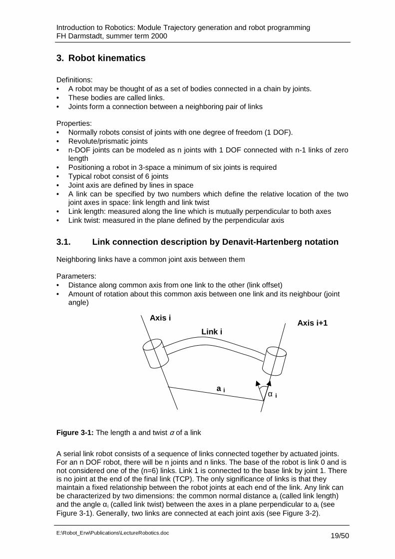
3.1. Link connection description by Denavit-Hartenberg notation
Neighboring links have a common joint axis between them
Parameters:• Distance along common axis from one link to the other (link offset)• Amount of rotation about this common axis between one link and its neighbour (joint
angle)
Figure 3-1: The length a and twist α of a link
A serial link robot consists of a sequence of links connected together by actuated joints.For an n DOF robot, there will be n joints and n links. The base of the robot is link 0 and isnot considered one of the (n=6) links. Link 1 is connected to the base link by joint 1. Thereis no joint at the end of the final link (TCP). The only significance of links is that theymaintain a fixed relationship between the robot joints at each end of the link. Any link canbe characterized by two dimensions: the common normal distance ai (called link length)and the angle αi (called link twist) between the axes in a plane perpendicular to ai (seeFigure 3-1). Generally, two links are connected at each joint axis (see Figure 3-2).
Axis i+1Axis i
Link i
a i α i
Introduction to Robotics: Module Trajectory generation and robot programmingFH Darmstadt, summer term 2000
E:\Robot_Erw\Publications\LectureRobotics.doc 20/50
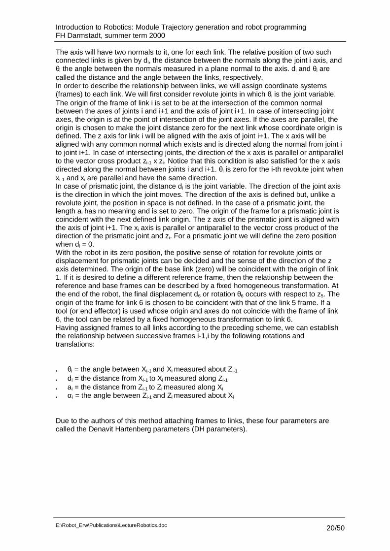
The axis will have two normals to it, one for each link. The relative position of two suchconnected links is given by di, the distance between the normals along the joint i axis, andθi the angle between the normals measured in a plane normal to the axis. di and θi arecalled the distance and the angle between the links, respectively.In order to describe the relationship between links, we will assign coordinate systems(frames) to each link. We will first consider revolute joints in which θi is the joint variable.The origin of the frame of link i is set to be at the intersection of the common normalbetween the axes of joints i and i+1 and the axis of joint i+1. In case of intersecting jointaxes, the origin is at the point of intersection of the joint axes. If the axes are parallel, theorigin is chosen to make the joint distance zero for the next link whose coordinate origin isdefined. The z axis for link i will be aligned with the axis of joint i+1. The x axis will bealigned with any common normal which exists and is directed along the normal from joint ito joint i+1. In case of intersecting joints, the direction of the x axis is parallel or antiparallelto the vector cross product zi-1 x zi. Notice that this condition is also satisfied for the x axisdirected along the normal between joints i and i+1. θi is zero for the i-th revolute joint whenxi-1 and xi are parallel and have the same direction.In case of prismatic joint, the distance di is the joint variable. The direction of the joint axisis the direction in which the joint moves. The direction of the axis is defined but, unlike arevolute joint, the position in space is not defined. In the case of a prismatic joint, thelength ai has no meaning and is set to zero. The origin of the frame for a prismatic joint iscoincident with the next defined link origin. The z axis of the prismatic joint is aligned withthe axis of joint i+1. The xi axis is parallel or antiparallel to the vector cross product of thedirection of the prismatic joint and zi. For a prismatic joint we will define the zero positionwhen di = 0.With the robot in its zero position, the positive sense of rotation for revolute joints ordisplacement for prismatic joints can be decided and the sense of the direction of the zaxis determined. The origin of the base link (zero) will be coincident with the origin of link1. If it is desired to define a different reference frame, then the relationship between thereference and base frames can be described by a fixed homogeneous transformation. Atthe end of the robot, the final displacement d6 or rotation θ6 occurs with respect to z5. Theorigin of the frame for link 6 is chosen to be coincident with that of the link 5 frame. If atool (or end effector) is used whose origin and axes do not coincide with the frame of link6, the tool can be related by a fixed homogeneous transformation to link 6.Having assigned frames to all links according to the preceding scheme, we can establishthe relationship between successive frames i-1,i by the following rotations andtranslations:
• θi = the angle between Xi-1 and Xi measured about Zi-1
• di = the distance from Xi-1 to Xi measured along Zi-1
• ai = the distance from Zi-1 to Zi measured along Xi
• αi = the angle between Zi-1 and Zi measured about Xi
Due to the authors of this method attaching frames to links, these four parameters arecalled the Denavit Hartenberg parameters (DH parameters).
Introduction to Robotics: Module Trajectory generation and robot programmingFH Darmstadt, summer term 2000
E:\Robot_Erw\Publications\LectureRobotics.doc 21/50
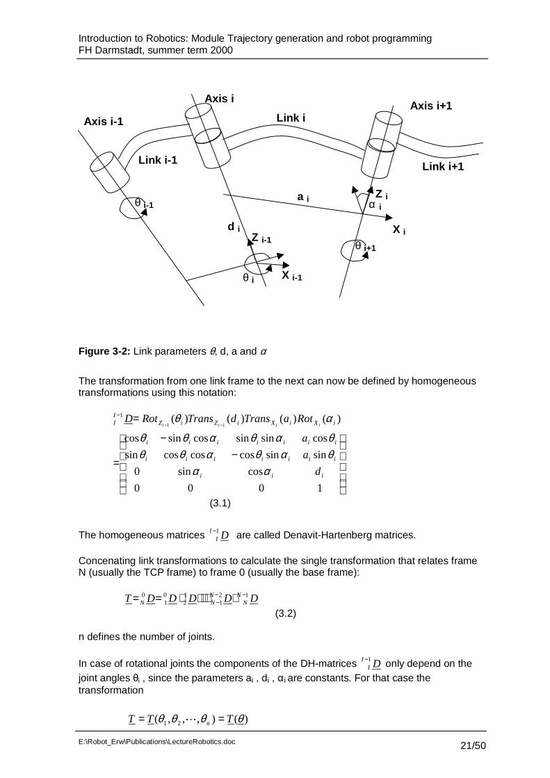
Figure 3-2: Link parameters θ, d, a and α
The transformation from one link frame to the next can now be defined by homogeneoustransformations using this notation:
−
−
=
=−−
−
1000
cossin0
sinsincoscoscossin
cossinsincossincos
)()()()(11
1
iii
iiiiiii
iiiiiii
iXiXiZiZII
d
a
a
RotaTransdTransRotDiiii
ααθαθαθθθαθαθθ
αθ
(3.1)
The homogeneous matrices DII1− are called Denavit-Hartenberg matrices.
Concenating link transformations to calculate the single transformation that relates frameN (usually the TCP frame) to frame 0 (usually the base frame):
DDDDDT NN
NNN
121
12
01
0 −−− ⋅⋅⋅⋅⋅==
(3.2)
n defines the number of joints.
In case of rotational joints the components of the DH-matrices DII1− only depend on the
joint angles θi , since the parameters ai , di , αi are constants. For that case thetransformation
)(),,,( 21 θθθθ TTT n == �
Link i+1
Axis i+1Axis i
Link i
Z i-1
X i-1
Z ia i
d i
θ i
Axis i-1
Link i-1
X i
α iθ i-1
θ i+1

Introduction to Robotics: Module Trajectory generation and robot programmingFH Darmstadt, summer term 2000
E:\Robot_Erw\Publications\LectureRobotics.doc 22/50
is a function of all joint angles. The joint angles can be formed to a vector:
=
nθ
θθ
θ �2
1
.
Examples2-dof robot with parallel axes
h1
h2
x
y
z
x
yz
y
x
z2
2
2 1
11
0
0 0Gelenk 1
Gelenk 2
TCP
Figure 3-3: Planar 2-dof robot including coordinate system
The following table shows the set of DH parameters: q1and q2 are variables (joint angles)
Joint θi / degree di Ai αi / degree1 0 0 h1 02 -90 0 h2 0
The DH-transformations are:
⋅−⋅−−−
=
⋅⋅−
=
1000
0100
cos0sincos
sin0cossin
1000
0100
sin0cossin
cos0sincos
2222
2222
12
1111
1111
01
qhqq
qhqq
Dqhqq
qhqq
D
ii
ii
qS
qCShCCSShSCCSCCSS
ChCSSChSSCCCSSC
qTDsin
cos
1000
010011)2121
(2021212121
11)2121(2021212121
)(02 =
=
++−−−+−+−−+−−−
==
2-dof robot with perpendicular axes
Introduction to Robotics: Module Trajectory generation and robot programmingFH Darmstadt, summer term 2000
E:\Robot_Erw\Publications\LectureRobotics.doc 23/50
x
z
xx
yy
y
zz
0
1
2
2
2
11
1
0
0
h
h2
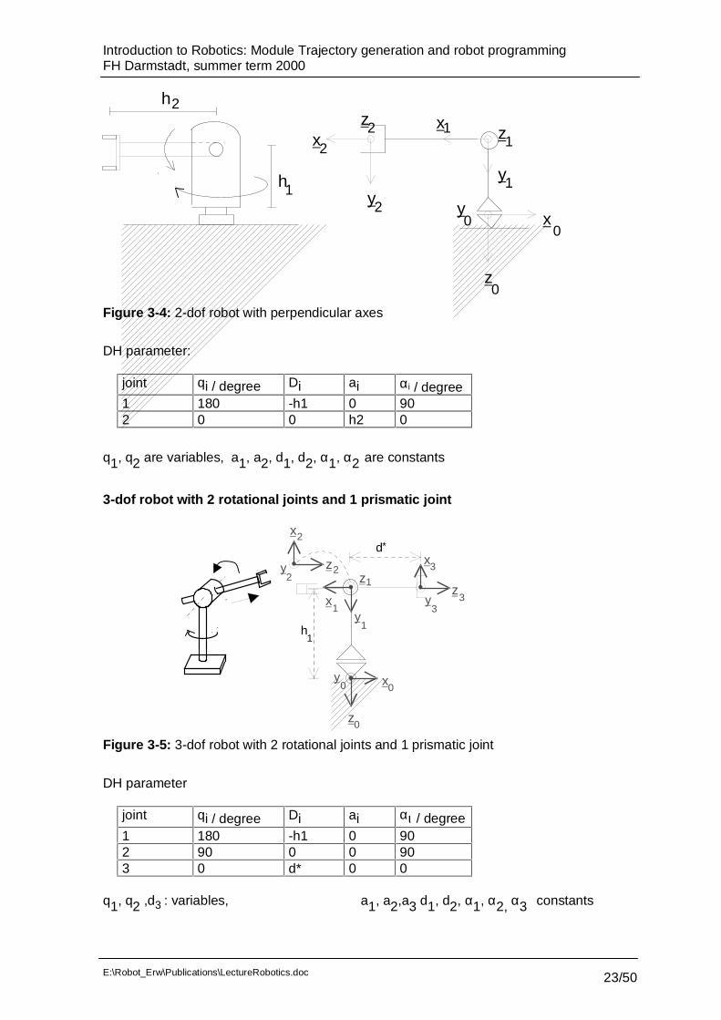
Figure 3-4: 2-dof robot with perpendicular axes
DH parameter:
joint qi / degree Di ai αi / degree1 180 -h1 0 902 0 0 h2 0
q1, q2 are variables, a1, a2, d1, d2, α1, α2 are constants
3-dof robot with 2 rotational joints and 1 prismatic joint
h
d
x
z
y
y
y
yx
x
zz
z
x
12
1
*
1
1
2
2
33
3
0
00
Figure 3-5: 3-dof robot with 2 rotational joints and 1 prismatic joint
DH parameter
joint qi / degree Di ai αι / degree1 180 -h1 0 902 90 0 0 903 0 d* 0 0
q1, q2 ,d3 : variables, a1, a2,a3 d1, d2, α1, α2, α3 constants

Introduction to Robotics: Module Trajectory generation and robot programmingFH Darmstadt, summer term 2000
E:\Robot_Erw\Publications\LectureRobotics.doc 24/50
6-dof robot with 6 rotational joints (frequently used kinematic structure)
x
yz
0
1
2
3
4
5
6
y
x
z
x
y
z
x
yz
x
x
x
z
z
y
y
0
1
1
2
zy
2
3
34
4
5
5
6
6
Figure 3-6: 6-dof robot with 6 rotational joints (frequently used kinematic structure)
xy
x x x
y yy
x
y
x
zy
yz
z
z z z
z
x
1
24
5 6
h
hh
h h
0
1
2
4 5 6
0
0
1
1
22
3
33 4
4 5
5 6
6
=0
Figure 3-7: sketch of 6-dof robot

Introduction to Robotics: Module Trajectory generation and robot programmingFH Darmstadt, summer term 2000
E:\Robot_Erw\Publications\LectureRobotics.doc 25/50
DH parameter:
Joint qi / degree di Ai αι / degree1 0 -h1(-0.78m) 0 902 -90 0 h2(0.8m) 03 0 0 0 -904 0 h4 (0.8m) 0 905 0 0 0 -906 0 h6 (0.334m) 0 0
Figure 3-8: Reis robot RV6 (payload 6 kg)
Introduction to Robotics: Module Trajectory generation and robot programmingFH Darmstadt, summer term 2000
E:\Robot_Erw\Publications\LectureRobotics.doc 26/50
y
x x
y y
x
zy
yz
z z z
z
x
10
4
6
h
2h
h
h
x0
1
2
4 5
y6
0
0
y1
z1
22
x3
33
4
4 5
5
x6 6
RV6
h11
5h =0
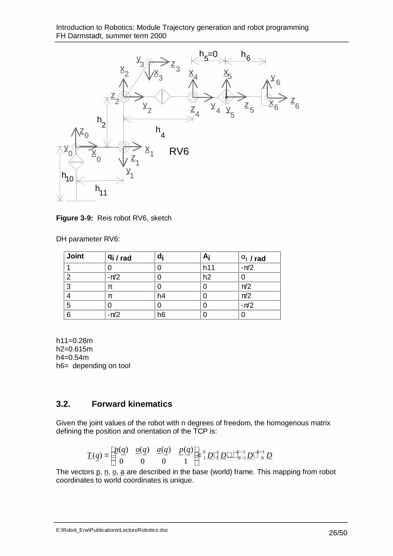
Figure 3-9: Reis robot RV6, sketch
DH parameter RV6:
Joint qi / rad di Ai αι / rad1 0 0 h11 -π/22 -π/2 0 h2 03 π 0 0 π/24 π h4 0 π/25 0 0 0 -π/26 -π/2 h6 0 0
h11=0.28mh2=0.615mh4=0.54mh6= depending on tool
3.2. Forward kinematics
Given the joint values of the robot with n degrees of freedom, the homogenous matrixdefining the position and orientation of the TCP is:
DDDDqpqaqoqn
qT NN
NN
121
12
01 ...
1000
)()()()()( −−
− ⋅⋅⋅⋅=
=
The vectors p, n, o, a are described in the base (world) frame. This mapping from robotcoordinates to world coordinates is unique.
Introduction to Robotics: Module Trajectory generation and robot programmingFH Darmstadt, summer term 2000
E:\Robot_Erw\Publications\LectureRobotics.doc 27/50
Roboter-koordinaten
Welt-koordinaten
q l m n p,, ,T q( )
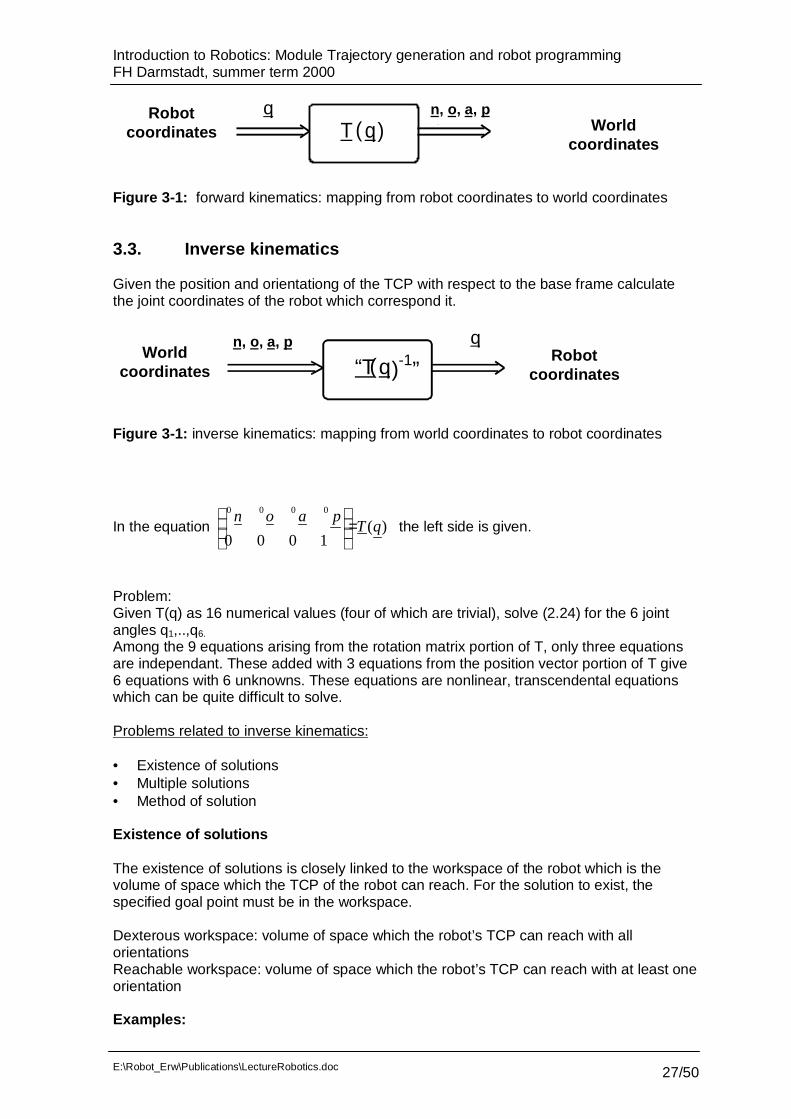
Figure 3-1: forward kinematics: mapping from robot coordinates to world coordinates
3.3. Inverse kinematics
Given the position and orientationg of the TCP with respect to the base frame calculatethe joint coordinates of the robot which correspond it.
Roboter-koordinaten
Welt-koordinaten
ql m n p,, ,“T q( )-1”
Figure 3-1: inverse kinematics: mapping from world coordinates to robot coordinates
In the equation )(1000
0000
qTpaon =
the left side is given.
Problem:Given T(q) as 16 numerical values (four of which are trivial), solve (2.24) for the 6 jointangles q1,..,q6.
Among the 9 equations arising from the rotation matrix portion of T, only three equationsare independant. These added with 3 equations from the position vector portion of T give6 equations with 6 unknowns. These equations are nonlinear, transcendental equationswhich can be quite difficult to solve.
Problems related to inverse kinematics:
• Existence of solutions• Multiple solutions• Method of solution
Existence of solutions
The existence of solutions is closely linked to the workspace of the robot which is thevolume of space which the TCP of the robot can reach. For the solution to exist, thespecified goal point must be in the workspace.
Dexterous workspace: volume of space which the robot’s TCP can reach with allorientationsReachable workspace: volume of space which the robot’s TCP can reach with at least oneorientation
Examples:
Robotcoordinates World
coordinates
n, o, a, p
Robotcoordinates
Worldcoordinates
n, o, a, p

Introduction to Robotics: Module Trajectory generation and robot programmingFH Darmstadt, summer term 2000
E:\Robot_Erw\Publications\LectureRobotics.doc 28/50
2 DOF robot with 21 ll =
Dexterous workspace: the originReachable workspace: disc of radius 21 ll +
2 DOF robot with 21 ll ≠
Dexterous workspace: emptyReachable workspace: ring of outer radius 21 ll + and inner radius 21 ll −
Since the 6 parameters are necessary to describe an arbitrary position and orientation ofthe TCP, the degree of freedom of the robot must be at least 6, in order a dexterousworkspace exists at all.
Multiple solutions:
Figure 3-2: Example for multiple solutions for a 2 DOF robot
Figure 3-3: example for infinite solutions
Suppose in example of
Lösung 2
Lösung 1
a
n
pq
q q
4
5 6
* =0q5

Introduction to Robotics: Module Trajectory generation and robot programmingFH Darmstadt, summer term 2000
E:\Robot_Erw\Publications\LectureRobotics.doc 29/50
Figure 3-3, that the given vectors p and n are realized by the joint angles
q q q q1 2 3 5 0* * * *, , , = . The orientation can be realized by an infinite numbrer of pairs q4 andq6 (normally by q4+q6 = 0). In practical implementations of the inverse kinematics anadditional condition will generate the solution, like
MINqqcqqc iiii
!2
,61,622
,41,41 )()( =−+− −−
This sum minimizes the travel range of q4 and q6 .
Method of solution:
There are two classes:• Closed form solutions (analytical, geometrical)• Numerical solutions
We concentrate in this lecture on closed form solutions.
Example : planar 2-dof robot:
Given )0()0(yx pandp as cartesian position. With
1121212)0(
1121212)0(
sin)sincoscos(sin
cos)sinsincos(cos
qhqqqqhp
qhqqqqhp
y
x
++=
+−=
the joint values q1 and q2 can be calculated. It depends on the kinematic structurewhether an analytical solution is possible.
Geometrical solution:
Law of cosine:
ab
ca b c b c2 2 2 2= + − ⋅ ⋅ ⋅cosα
Example: planar 2-dof robot (Figure 3-4)
Introduction to Robotics: Module Trajectory generation and robot programmingFH Darmstadt, summer term 2000
E:\Robot_Erw\Publications\LectureRobotics.doc 30/50
h
qp
P
x0
y0
qh
2
1
1
2
α
β
χ
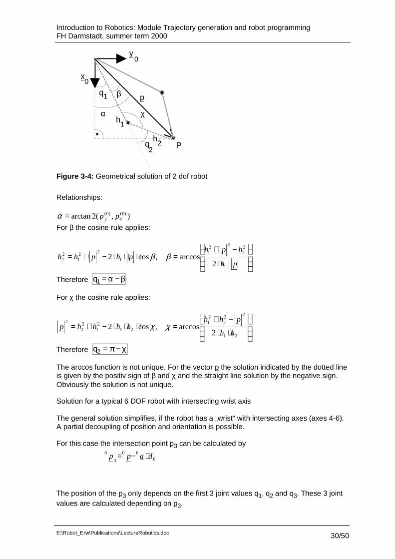
Figure 3-4: Geometrical solution of 2 dof robot
Relationships:
),(2arctan )0()0(xy pp=α
For β the cosine rule applies:
⋅⋅
−+=⋅⋅⋅−+=
ph
hphphphh
1
22
221
1
221
22
2arccos,cos2 ββ
Therefore q1 = −α β
For χ the cosine rule applies:
⋅⋅
−+=⋅⋅⋅−+=
21
222
21
212
122
2
2arccos,cos2
hh
phhhhhhp χχ
Therefore q2 = −π χ
The arccos function is not unique. For the vector p the solution indicated by the dotted lineis given by the positiv sign of β and χ and the straight line solution by the negative sign.Obviously the solution is not unique.
Solution for a typical 6 DOF robot with intersecting wrist axis
The general solution simplifies, if the robot has a „wrist“ with intersecting axes (axes 4-6).A partial decoupling of position and orientation is possible.
For this case the intersection point p3 can be calculated by
600
3
0 dapp ⋅−=
The position of the p3 only depends on the first 3 joint values q1, q2 and q3. These 3 jointvalues are calculated depending on p3.

Introduction to Robotics: Module Trajectory generation and robot programmingFH Darmstadt, summer term 2000
E:\Robot_Erw\Publications\LectureRobotics.doc 31/50
Calculation of q3 :
z0
x0
R
p
3
3d
ll2
1
1 q3ϕ
Figure 3-5: Calculation of q3
ϕπϕ
ϕϕ
−=⋅⋅
−+=
⋅⋅⋅−+=
+++=
+=
2 :known is q re therefo
2arccos
cos2::for cosine of law
)(,0
0
3321
2
322
21
2122
21
2
3
213
23
233
1
33
qll
Rll
llllR
dpppR
d
pR zyx
Calculation of q2 :
z0
x0
p
R3
3d
ll2
1
1 q2
-
12 β
β
Figure 3-6: Calculation of q2

Introduction to Robotics: Module Trajectory generation and robot programmingFH Darmstadt, summer term 2000
E:\Robot_Erw\Publications\LectureRobotics.doc 32/50
)( :known is q e therefor2
arccos
cos2 :for cosine of law
arcsinsin
212231
22
2
32
12
231
2
321
222
3
131
3
131
βββ
ββ
ββ
+−=⋅⋅
−+=
⋅⋅⋅−+=
−=
−=
qRl
lRl
RlRll
R
dp
R
dp zz
Calculation of q1 :
Figure 3-7: Calculation of q1
q p py x1 3 32= arctan ( , )Calculation of q5 :
Figure 3-8: Calculation of q5
)arccos( 35 azq •=
Calculation of q4:
[ ][ ] TDDDDDD
TDDDDT
DDDDDDT
⋅⋅⋅=⋅⋅
⇒⋅=⇒⋅=
⋅⋅⋅⋅⋅=
−
−
123
12
01
56
45
34
103
36
36
03
56
45
34
23
12
01
The right side of the last equation is known, since T is given and the Denavit-Hartenbergmatrices at the right side only depend on q1, q2, q3 , which now available. The left sidedepends only q4, q5 and q6. The modulus of q5 is also available. It is possible to eliminateq6 and to calculate q4 .
z0
x0
p3
z
x
z
a
3
3
3
a
z3
q5

Introduction to Robotics: Module Trajectory generation and robot programmingFH Darmstadt, summer term 2000
E:\Robot_Erw\Publications\LectureRobotics.doc 33/50
Calculation of q6:
Figure 3-9: Calculation of q6
=
•=
1000D
,...,qgiven by the calculated becan Dsince known, is
)arccos(
5
05
0
5
05
005
51055
0
5
06
pzyx
qy
oyq
z5
x
y
n
o
a
q6
5
5

Introduction to Robotics: Module Trajectory generation and robot programmingFH Darmstadt, summer term 2000
E:\Robot_Erw\Publications\LectureRobotics.doc 34/50
4. Trajectory Generation
Scope: methods of computing a trajectory in multidimensional space
Definition: trajectory refers to a time history of position, velocity and acceleration for eachdegree of freeom
Issues:• Specification of trajectories• Motion description easy for robot operators• start and end point• geometrical properties• Representation of trajectories in the robot control• Computing trajectories on-line (at run time)
General considerations
• Motion of robot is described as motion of TCP (tool frame)• Supports robot operator’s imagination• Decoupling the motion description from any robot, end-effector (modularity)• Exchangeability with other robots• Supports the idea of moving frames (conveyer belt)
Basic problem: move the robot from the start position, given by the tool frame Tinitial to theend position given by the tool frame Tfinal.
Spatial motion constraints:• Specification of motion might include socalled via points• Via points: intermediate points between start and end points
Temporal motion contraints:• Specification of motion might include elapsed time between via points
Requirements:• Execution of smooth motions• Smooth (motion) function: function and its first derivative is continous• Jerky motions increase wear on the mechanism (gears) and cause vibrations by
exciting resonances of the robot.
There are two methods of path generation:
• Joint space schemes: path shapes in space and time are described in terms offunctions of joint angles. This motion type is named Point-to-Point motion (PTP)
• Cartesian space schemes: path shapes in space and time are described in terms offunctions of cartesian coordinates. This motion type is named Continous Path motion(CP)
4.1. Trajectory generation in joint space (PTP motions)

Introduction to Robotics: Module Trajectory generation and robot programmingFH Darmstadt, summer term 2000
E:\Robot_Erw\Publications\LectureRobotics.doc 35/50
• Path shape (in space and time) described in terms of functions of joint angles• Description of path points (via points plus start and end point) in terms of tool frames• Each path point is converted into joint angles by application of inverse kinematics• Identifying a smooth function for each of the n joints passing through the via points
and ends at the target point• Synchronisation of motion (each joint starts and ends at the same time)• Joint which travels the longest distance defines the travel time (assuming same
maximal acceleration for each joint)
• In between via points the shape of the path is complex if described in cartesian space• Joint space trajectory generation schemes are easy to compute• Each joint motion is calculated independantly from other joints
.
no
q q5 6
q4
a
A: Start B: Ziel
Figure 4-1: PTP motion between two points
Many, actually infinite, smooth functions exist for such motions
Four contraints on the (single) joint function q(t) are evident:
• Start configuration Aqq =)0( , end configuration Bend qtq =)(
• Velocities 0)0( =q�
, 0)( =endtq�
Four constraints can be satisfied by a polynomial of degree 3 or higher.
In case of via points the velocity is not zero.
• Start configuration Aqq =)0( , end configuration Bend qtq =)(
• Velocities 0)0( qq��
= , endend qtq��
=)(
Choosing velocities by
• robot user• automatically chosen by the robot control
Using these type of polynomials does not in general generate time optimal motions
Introduction to Robotics: Module Trajectory generation and robot programmingFH Darmstadt, summer term 2000
E:\Robot_Erw\Publications\LectureRobotics.doc 36/50
Linear function with parabolic blends:
q(t)
q(t)
q(t)
tbt
tftf-tbt0t
tht
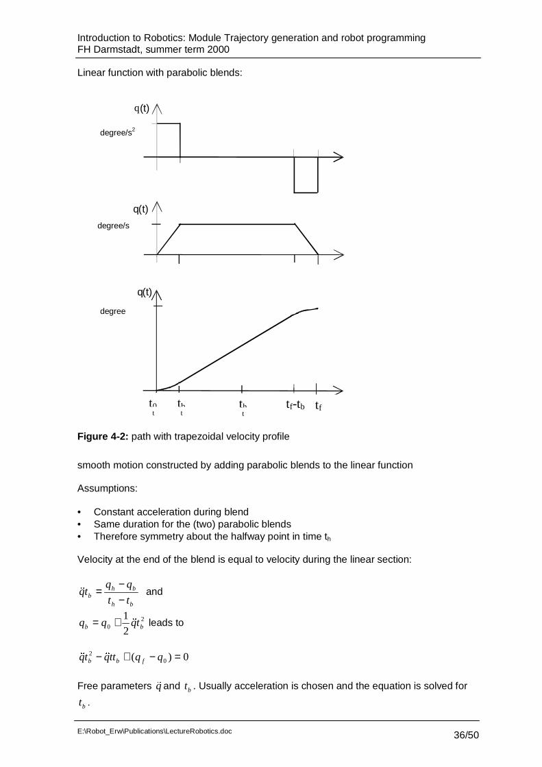
Figure 4-2: path with trapezoidal velocity profile
smooth motion constructed by adding parabolic blends to the linear function
Assumptions:
• Constant acceleration during blend• Same duration for the (two) parabolic blends• Therefore symmetry about the halfway point in time th
Velocity at the end of the blend is equal to velocity during the linear section:
bh
bhb tt
qqtq
−−
=��
and
20 2
1bb tqqq
��
+= leads to
0)( 02 =−+− qqttqtq fbb
����
Free parameters q��
and bt . Usually acceleration is chosen and the equation is solved for
bt .
degree/s2
degree
degree/s

Introduction to Robotics: Module Trajectory generation and robot programmingFH Darmstadt, summer term 2000
E:\Robot_Erw\Publications\LectureRobotics.doc 37/50
• Acceleration must be sufficiently high (otherwise a solution does not exist)• Acceleration is not continous, which excites vibrations
Alternative: sinoidal profile
Acceleration defined by:
⋅⋅= t
tqtq
b
π2max sin)(
����
(4.1)
q(t)
q(t)
q(t)
tb
tb
tv
tv
tE
tE
tv tEtb
t
t
t
Figure 4-3: profile for a sinusoidal path
The following relationships are valid:
maxmax
2max
maxmax
2max
2max
max ,2
,2164 q
qtt
qtq
qqqtqtq f
fbff
fff��
�
��
������
�
−=−⋅
⋅=
⋅−
⋅−
⋅=
bfvb tttq
qt −=
⋅= ,
2
max
max��
�
(4.2)
The constraint on the acceleration is
ff qqt ⋅≥⋅ 8max2 ��
(4.3)
Calculation of q(t):
Introduction to Robotics: Module Trajectory generation and robot programmingFH Darmstadt, summer term 2000
E:\Robot_Erw\Publications\LectureRobotics.doc 38/50
−⋅−+−−⋅+−⋅⋅=≤≤
⋅−⋅=≤≤
−⋅+⋅=≤≤
))(2
cos(14222
)(:
2
1)(:
12
cos84
1)(:0
2
22
22max
max
2
22
max
vb
bb
fbfffv
bvb
b
bb
ttt
tt
ttt
ttt
qtqttt
ttqtqttt
tt
ttqtqtt
ππ
ππ
��
�
��
(4.4)
4.1.1. Asynchrone PTP
independant calculation of joint angles along each pathdifferent travel time for each axis in general (misbehaviour)
• for each joint the values max0 ,, qqq f
��
are given. The travel time ti for each joint is
calculated
4.1.2. Synchrone PTP:
each joint ends its motion at the same time
• for each joint the values max0 ,, qqq f
��
are given. The travel time ti for each joint is
calculated• calculate the maximum travel time { }if
dofif tt ,
,..,1max, max
==
• for each joint set max,, fif tt =• adjust joint speeds iqmax,
�
0max,,21
max,max,max,212
max,max,
max,
max,
,max,, =⋅+⋅⋅−⇒+== iiffiii
i
i
i
iffif qqtqqq
q
q
q
qtt
and therefore
16
8
4max,,
2max,
2max,max,max,
max,iiffifi
i
qqtqtqq
⋅−⋅−
⋅=
����
�
(4.5)
The negative sign of the square root has to be chosen in order to fulfill 2tb<tf,max
4.2. Trajectory generation in cartesian space
robot user would like to control the motion between start and end pointseveral possibilities:
• straight line motion (TCP follows a straight line)• circular motion (TCP follows a circle segment)• spline motion
Introduction to Robotics: Module Trajectory generation and robot programmingFH Darmstadt, summer term 2000
E:\Robot_Erw\Publications\LectureRobotics.doc 39/50
• inverse kinematics needs to be calculated at run time• computational expensive (depending on the robot)
issues:• interpolation of TCP position (linear change of coordinates)• interpolation of orientation (linear change of matrix elements would fail)
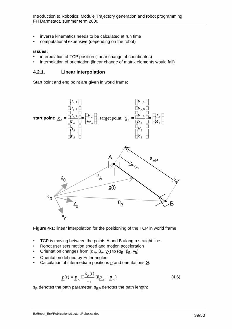
4.2.1. Linear Interpolation
Start point and end point are given in world frame:
start point: point target ,
,
,
,
,
,
Θ
=
=
Θ
=
=B
B
B
B
B
Bz
By
Bx
BA
A
A
A
A
Az
Ay
Ax
A
pp
p
p
xpp
p
p
x
χβα
χβα
p(t)
K
A
B
x0
z0
y0
pA
pB
sP
0
EPs
Figure 4-1: linear interpolation for the positioning of the TCP in world frame
• TCP is moving between the points A and B along a straight line• Robot user sets motion speed and motion acceleration• Orientation changes from (αA, βA, γA) to (αB, βB, γB)
• Orientation defined by Euler angles• Calculation of intermediate positions p and orientations Θ:
)()(
)(AB
f
p
App
s
tsptp −⋅+= (4.6)
sP denotes the path parameter, sEP denotes the path length:

Introduction to Robotics: Module Trajectory generation and robot programmingFH Darmstadt, summer term 2000
E:\Robot_Erw\Publications\LectureRobotics.doc 40/50
2,,
2,,
2,, )()()( AzBzAyByAxBxABfP pppppppps −+−+−=−=
(4.7)
The motion starts at time t=0 and ends in the target at time t=tEP.
0)(s )0( P == fPP ts��
.
Orientation:
Θ Θ Θ ΘΘ
Θ( )
( )( )t
s tsA
EB A= + ⋅ −
222 )()()( ABABABABfs χχββαα −+−+−=Θ−Θ=Θ
(4.8)
0)(s )0( == ΘΘΘ Ets��
For the positioning of the TCP velocity profiles like in the PTP case are used
• Trapezoidal profile• Sinusoidal profile
Robot user sets speed and acceleration for position and orientationThe duration of the motion (in case of sinusoidal profile) is:
Θ
Θ
Θ
ΘΘ +=+=
b
v
v
st
b
v
v
st f
fP
P
P
fPfP and
(4.9)
Synchronisation of motion:
),( Θ= ffPf ttMaxt .
Case 1: tf = tfP
Θ
ΘΘΘΘ
ΘΘΘ =⋅−
⋅−
⋅=
b
vbs
tbtbv ff
b
22
t, 42
.
(4.10)
Case 2: tf = tfΘ
P
PPP
fPfPP b
vbs
tbtbv =⋅−
⋅−
⋅= bP
22
t, 42
.
(4.11)
Reference to the PTP motion:

Introduction to Robotics: Module Trajectory generation and robot programmingFH Darmstadt, summer term 2000
E:\Robot_Erw\Publications\LectureRobotics.doc 41/50
)()( )()(
)()(or )()(
)(ss(t) )()(
,, ,,
max
max
tbtbtbtq
tvtvtvtq
ttstq
tttttttt
mP
mP
P
VbVbVPbPVb
Θ
Θ
Θ
ΘΘ
→→→→
→→→→
��
�
The following scheme presents the algorithm for straight line motions

Introduction to Robotics: Module Trajectory generation and robot programmingFH Darmstadt, summer term 2000
E:\Robot_Erw\Publications\LectureRobotics.doc 42/50
pA A
pB B
P
, , ,
PvPb v b, ,,
sf P tbP tbtf P tf, sf, , ,
tf
tf P
< 2 tb
< tbP2Pv tbP tf P, ,
tf P tf>
Pv tbP,
t f =tf P
, tbv
t f = tf
s s(t)
(t)
(t)
p (t)
l(t), m(t), n(t)(t)
q (t)d
ΘΘ
Θ
Θ
ΘΘ
Correction ofv t tΘ ΘΘb f, ,
Θ
Θ
Θ
ΘΘ
Θ Θ
Θ
Calculation of
yes
no
no
Calculation of
to
Transformation from
inverse kinematics
yesCorrection of
Correction ofCorrection of

Introduction to Robotics: Module Trajectory generation and robot programmingFH Darmstadt, summer term 2000
E:\Robot_Erw\Publications\LectureRobotics.doc 43/50
Problems related to cartesian motions:
• Intermediate points unreachable (out of work space)• High joint rates near singularities• Start and target position reachable in different solutions
4.2.2. Circular interpolation
Motion of the TCP along a circular segment from point P1 via P2 to point P3.P2 is sometimes called auxiliary point.The points P1,P2,P3 and the velocity vC and acceleration bC are defined by the robot user.
• from points P1,P2,P3 calculate center point M and radius r by
)()( 2312 PPPPnK −×−=�
.
E X P x n d x OXi i i= ∈ ⋅ = = →
{ | , : }3 ��� �
for i=1,2 with 2322
12232
12121
1121
)(:),(:
)(:),(:
nPPdPPn
nPPdPPn��
��
⋅+=−=⋅+=−=
The vector �
m of the center point M is the solution of the linear system
�
�
�
�
n
n
n
m
d
d
d
T
T
KT
K
1
2
1
2
=
,
• introduction of path parameter sC(t) = r*ϕ(t), where ϕ(t) is opening angle up to actual
position. sCE = r*ϕG denotes the total path length.
• analog procedure to linear interpolation
Exercise:
Given the points P1,P2,P3 defining a circular segment, withP1 = [0 1 1]T; P2 = [1 1 2]T; P3 = [2 1 1]T Calculate center point M and radius r.

Introduction to Robotics: Module Trajectory generation and robot programmingFH Darmstadt, summer term 2000
E:\Robot_Erw\Publications\LectureRobotics.doc 44/50
r 1 r2 r3
xC
yC
M
P1
P2
P3
S (t)C
pC
p
rM
p12
p13
x0
y0
z0
K0
R
p23
ϕϕM
G
4.2.3. Corner smoothing
The above mentioned interpolation methods let the motion stop at the end pointCorner smoothing let the robot move from one segment to another without reducing speed
Introduction to Robotics: Module Trajectory generation and robot programmingFH Darmstadt, summer term 2000
E:\Robot_Erw\Publications\LectureRobotics.doc 45/50
4.2.4. Spline interpolation based on Bézier curves
• Bezier curves are useful to design trajectories with certain „roundness“ properties• Defined by a series of control points with associated weighting factors• Weighting factors „pull“ the curve towards the control points• Bezier curves are based on Bernstein polynomials (we consider here cubic
polynomials, n=3)
B un
ku uk
n n k k( ): ( )=
− −1
with normalized parameter interval.
Bernstein polynomials can be derived from formula:
1 1 10
= − + =
∑ −
=
−( ( ) ) ( )u un
ku un
k
nn k k
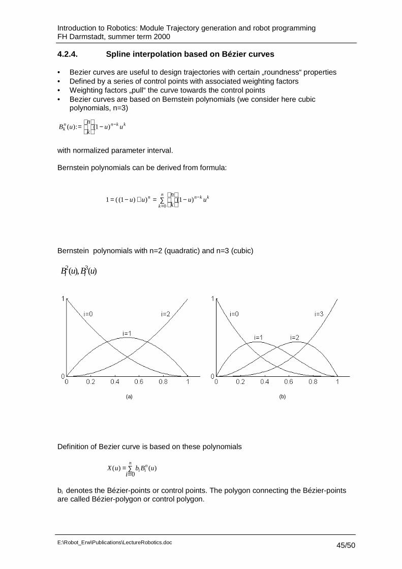
Bernstein polynomials with n=2 (quadratic) and n=3 (cubic)
B u B ui i
2 3( ), ( )
(a) (b)
Definition of Bezier curve is based on these polynomials
X u b B ui
i in
n( ) ( )=
=∑
0
bi denotes the Bézier-points or control points. The polygon connecting the Bézier-pointsare called Bézier-polygon or control polygon.
Introduction to Robotics: Module Trajectory generation and robot programmingFH Darmstadt, summer term 2000
E:\Robot_Erw\Publications\LectureRobotics.doc 46/50
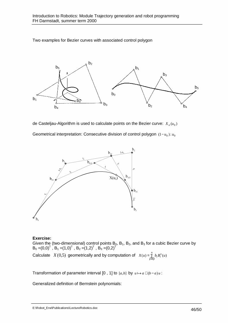
Two examples for Bezier curves with associated control polygon
de Casteljau-Algorithm is used to calculate points on the Bezier curve: X un ( )0
Geometrical interpretation: Consecutive division of control polygon ( ) :1 0 0− u u
Exercise:Given the (two-dimensional) control points B0, B1, B2, and B3 for a cubic Bezier curve byB0 =(0,0)T , B1 =(1,0)T , B2 =(1,2)T , B3 =(0,2)T
Calculate )5,0(X geometrically and by computation of X u b B ui
i in
n( ) ( )=
=∑
0
Transformation of parameter interval [0 , 1] to [ , ]a b by u a b a u� + −( ) :
Generalized definition of Bernstein polynomials:
b4b2
b3
b5
b1
b0
b4
b0
b5
b3
b2
b1
Introduction to Robotics: Module Trajectory generation and robot programmingFH Darmstadt, summer term 2000
E:\Robot_Erw\Publications\LectureRobotics.doc 47/50
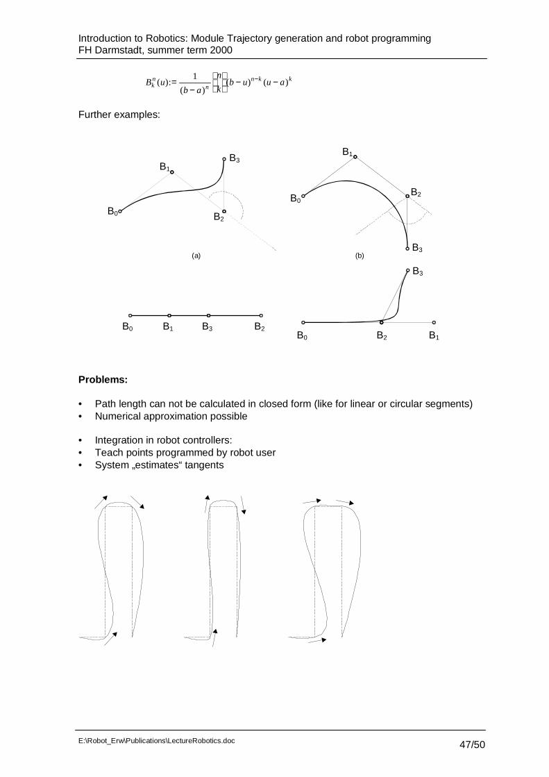
B ub a
n
kb u u ak
nn
n k k( ):( )
( ) ( )=−
− −−1
Further examples:
(a) (b)
Problems:
• Path length can not be calculated in closed form (like for linear or circular segments)• Numerical approximation possible
• Integration in robot controllers:• Teach points programmed by robot user• System „estimates“ tangents
B2
B3B1
B0
B2
B3
B3
B1
B0
B0 B1 B3 B2B0 B2 B1

Introduction to Robotics: Module Trajectory generation and robot programmingFH Darmstadt, summer term 2000
E:\Robot_Erw\Publications\LectureRobotics.doc 48/50
Synchronisation with orientation:
Generic trajectory generation (example linear interpolation):
B P
B P P P
B P P P
B P
A
A E A
E E A
E
0
113
213
3
:
: ( )
: ( )
:
=
= + −
= − −=
�
e y
�
ez
�
ex
�
e y
�
ez
�
ex
�
e y
�
ez�
ex
PP
P
�
e y
�
ez�
ex
Introduction to Robotics: Module Trajectory generation and robot programmingFH Darmstadt, summer term 2000
E:\Robot_Erw\Publications\LectureRobotics.doc 49/50
5. Robot programming languages
Robot programming systems are the interface between the robot and the human user.The sophistication of such an user interface is becoming very important as robots areapplied to more and more demanding industrial applications.In considering the programming of manipulators, it is important to remember that they aretypically only a minor part of an automated process. The term workcell is used to describea local collection of equipment which may include one or more robots, conveyor systems,part feeders and fixtures. At the next higher level, workcells might be interconnected infactorywide networks so that a central control computer can control the overall factoryflow.
5.1. Levels of robot programming
Three levels of robot programming exist:
• Teach In programming• Explicit robot languages• Task level programming languages
Teach In programming
The robot will be moved by the human user through interaction with a teach pendant(sometimes called teach box). Teach pendant are hand-held button boxes which allowcontrol of each robot joint or of each cartesian degree of freedom. Todays controllersallow alphanumeric input, testing and branching so that simple programs involving logiccan be entered.
Explicit robot languages
With the arrival of inexpensive and powerful computers, the trend has been increasinglytoward programming robots via programs written in computer programming languages.Usually these computer programming languages have special features which apply to theproblems of programming robots. An international standard has been established with theprogramming language IRL (Industrial Robot Language, DIN 66312)
Task level programming
The third level of robot programming methodology is embodied in task-level programminglanguages. These are languages which allow the user to command desired subgoals ofthe task directly, rather than to specify the details of every action the robot is to take. Insuch a system, the user is able to include instructions in the application program at asignificantly higher level than in an explicit programming language. A task-levelprogramming system must have the ability to perform many planning tasks automatically.For example, if an instruction to grasp the bolt is issued, the system must plan a path ofthe manipulator which avoids collision with any surrounding obstacles, automaticallychoose a good grasp location on the bolt, and grasp it. In contrast, in an explicit robotlanguage, all these choices must be made by the programmer.
The border between explicit robot programming languages is quite distinct. Incrementaladvances are beeing made to explicit robot programming languages which help to easeprogramming, but these enhancements cannot be counted as components of a task-levelprogramming system. True task-level programming of robots does not exist yet inindustrial controllers but is an active topic of research.
Introduction to Robotics: Module Trajectory generation and robot programmingFH Darmstadt, summer term 2000
E:\Robot_Erw\Publications\LectureRobotics.doc 50/50
5.2. Requirements of a robot programming language
Important requirements of a robot programming language are:
• World modeling• Motion specification• Flow of execution• Sensor inegration
World modeling:
• Existence of geometric types to present• Joint angle sets• Cartesian positions• Orientations• Representation of frames
• Ability to to do math on on structured types like frames, vectors and rotation matrices• Ability to describe geometric entities like frames in several different convenient
representations with the ability to convert between representations
Motion execution:
• Description of desired motion (motion type, velocity, acceleration)• Specifications of via points, goal points, corner smoothing parameters• Ability to specify goals relative to various frames, including frames defined by the user
and frames in motion (on a conveyor for example)
Flow of execution:
• Support of concepts like testing and branching• Looping, calls to subroutines• Parallel processing, signal and wait primitives• Interrupt handling
Sensor integration:
• Interaction with sensors• Integration with vision systems• Sensor to track the conveyor belt motion• Force torque sensor for force control strategies