Introduction to programming with Matlab/Python Lecture 1€¦ · Introduction to programming with...
20
Introduction to programming with Matlab/Python — Lecture 1 Brian Thorsbro Department of Astronomy and Theoretical Physics, Lund University, Sweden. Monday, October 30, 2017
Transcript of Introduction to programming with Matlab/Python Lecture 1€¦ · Introduction to programming with...
Introduction to programmingwith Matlab/Python
— Lecture 1
Brian Thorsbro
Department of Astronomyand Theoretical Physics,Lund University, Sweden.
Monday, October 30, 2017
Courses
These lectures are a mini-series companion to:
ASTM13 Dynamical Astronomy
ASTM21 Statistical tools in Astrophysics
Matlab installed in the lab (Lyra). Personal laptops are OK!Install Matlab from: http://program.ddg.lth.se/Install Python3 from: https://www.anaconda.com/download/
Brian Thorsbro 1/19
Outline
Content in this lecture:
I Matlab
I Python/Spyder
I The Hertzsprung-Russell diagram(example computational task)
I Basic machine architecture
I Data representation
I Data manipulation
Brian Thorsbro 2/19

Matlab
Install from: http://program.ddg.lth.se/
Brian Thorsbro 3/19
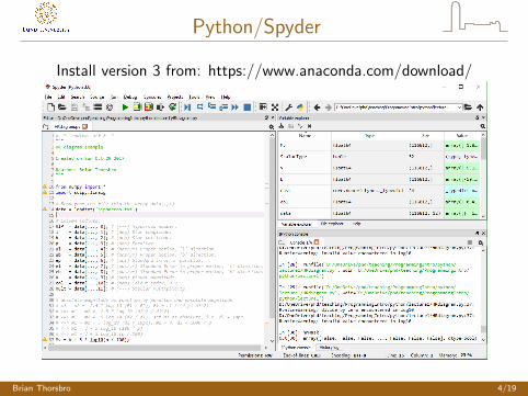
Python/Spyder
Install version 3 from: https://www.anaconda.com/download/
Brian Thorsbro 4/19

The HR diagram
(from http://www.astronomynotes.com)
Brian Thorsbro 5/19

The task at hand
The task at hand:
I Load the Hipparcos database(about 120000 stars)
I Plot the stars in a HR diagram
But first: Machine architecture
Brian Thorsbro 6/19

Basic Machine Architecture
(from http://en.wikibooks.org)
Brian Thorsbro 7/19

The Hipparcos Database
The Hipparcos database:
I HIP - primary key / identifier
I l - Star longitude (deg)
I b - Star latitude (deg)
I p - Parallax (mas)
I ul - Proper motion, ’l’ direction (mas/yr)
I ub - Proper motion, ’b’ direction (mas/yr)
I ep - Standard Error in parallax (mas)
I el - Standard Error in proper motion, ’l’ direction (mas/yr)
I eb - Standard Error in proper motion, ’b’ direction (mas/yr)
I V - Visual magnitude (mag)
I col - Colour index, B-V (mag)
I mult - Stellar multiplicity, i.e. binaries etc.
Brian Thorsbro 8/19

Data representation
Computers work with on or off, i.e. bits: 1 or 0.
However, there are different conventions for how data can bestored using combinations of these ones and zeroes.
The number 10 can be represented in multiple ways:
I Integer (10): 0 0000000000000000000000000001010
I Double (1.0 · 101): 0 100000000100100000000000000000000000000000000000000000000000000
I ASCII String (”10”): 00110001 00110000
In science you normally want to work with doubles. In Matlab thisis automatic, in Python and many other programming languagesalways include at least one decimal, i.e. type 10.0 — good idea tomake this a habit.
Brian Thorsbro 9/19

Advanced data structures
We like to work on big data sets with many numbers Toaccommodate that Matlab and Python lets us group up thenumbers in multidimensional arrays.
Matlab:
myMatrix = [ 17 15 ; 13 11 ];
val = myMatrix(1,2);
row = myMatrix(1,:);
col = myMatrix(:,2);
Python (with numpy library):
myMatrix = array([[17.0,15.0],[13.0,11.0]])
val = myMatrix[0,1]
row = myMatrix[0,...]
col = myMatrix[...,1]
Brian Thorsbro 10/19

The database file
Brian Thorsbro 11/19

File to memory
Data in the file is in text format (like ASCII string) with a spacebetween the numbers. Matlab and Python provides methods to doautomatic conversion for you.
Matlab:
data = dlmread(’hipparcos.txt’);
Python (with numpy library):
data = loadtxt(’hipparcos.txt’)
In both cases “data” is then a matrix of 116812x12 doubles(rows x columns — really cool).
Brian Thorsbro 12/19

Data refinement
With data loaded we can start refining it. First extract the usefuldata from the big loaded data matrix:
Matlab:
p = data(:, 4); % (mas) Parallax.
V = data(:,10); % (mag) Visual magnitude.
col = data(:,11); % (mag) Colour index, B-V.
Python (with numpy library):
p = data[..., 3] # (mas) Parallax.
V = data[..., 9] # (mag) Visual magnitude.
col = data[...,10] # (mag) Colour index, B-V.
However, the absolute magnitude is not stored in the database. Ithas to be calculated.
Brian Thorsbro 13/19

Absolute magnitude
Absolute magnitude is the magnitude a star would have were itplaced at a distance of 10 pc. Thus by definition of astronomicalmagnitudes for stars:
Mv − V = −5 · log10
(d
10pc
),
with the distance determined by using the parallax:
d =1000pc
p,
thus
Mv = V + 5 · log10
( p
100
).
Brian Thorsbro 14/19
Data refinement
Even though our visual apparent magnitude and parallaxes are inarrays, the actual calculation is quite simple:
Matlab:
Mv = V + 5 * log10(p / 100);
Python (with numpy library):
Mv = V + 5 * log10(p / 100)
The resulting “Mv” variable is thus also an array with the samedimensions.
Brian Thorsbro 15/19
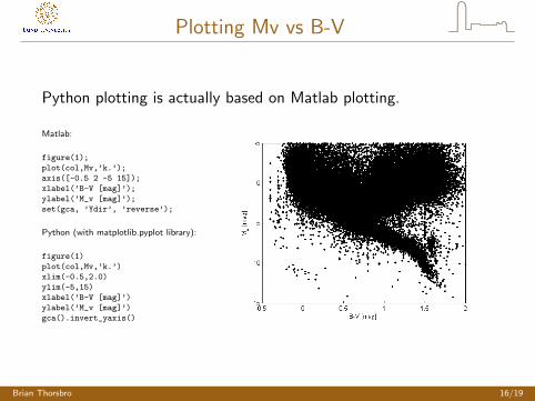
Plotting Mv vs B-V
Python plotting is actually based on Matlab plotting.
Matlab:
figure(1);
plot(col,Mv,’k.’);
axis([-0.5 2 -5 15]);
xlabel(’B-V [mag]’);
ylabel(’M_v [mag]’);
set(gca, ’Ydir’, ’reverse’);
Python (with matplotlib.pyplot library):
figure(1)
plot(col,Mv,’k.’)
xlim(-0.5,2.0)
ylim(-5,15)
xlabel(’B-V [mag]’)
ylabel(’M_v [mag]’)
gca().invert_yaxis()
Brian Thorsbro 16/19

Plotting Mv vs B-V
Only plotting stars with small parallax error (max 5% error).
Matlab:
figure(2);
plot(col(p>20*ep),Mv(p>20*ep),’k.’);
axis([-0.5 2 -5 15]);
xlabel(’B-V [mag]’);
ylabel(’M_v [mag]’);
set(gca, ’Ydir’, ’reverse’);
Python (with matplotlib.pyplot library):
figure(2)
plot(col[p>20*ep],Mv[p>20*ep],’k.’);
xlim(-0.5,2.0)
ylim(-5,15)
xlabel(’B-V [mag]’)
ylabel(’M_v [mag]’)
gca().invert_yaxis()
Note: Parallax error maps non-linearly to distance due tod = 1000/p [pc]!
Brian Thorsbro 17/19

Plotting Mv vs B-V
Possible to build up selection masks.
Matlab:
hrMask = (p>20*ep) & (mult==0);
figure(3);
plot(col(hrMask),Mv(hrMask),’k.’);
axis([-0.5 2 -5 15]);
xlabel(’B-V [mag]’);
ylabel(’M_v [mag]’);
set(gca, ’Ydir’, ’reverse’);
Python (with matplotlib.pyplot library):
hrMask = (p>20*ep) & (mult==0)
figure(3)
plot(col[hrMask],Mv[hrMask],’k.’)
xlim(-0.5,2.0)
ylim(-5,15)
xlabel(’B-V [mag]’)
ylabel(’M_v [mag]’)
gca().invert_yaxis()
Brian Thorsbro 18/19

The End
Questions?
Brian Thorsbro 19/19