Introduction to Programming and Computing for Scientists · Introduction to Programming and...

Introduction to Programming and Computing for Scientists

Oxana Smirnova

Lund University

Lecture 5

Oxana Smirnova (Lund University) Programming for Scientists Lecture 5 1 / 47

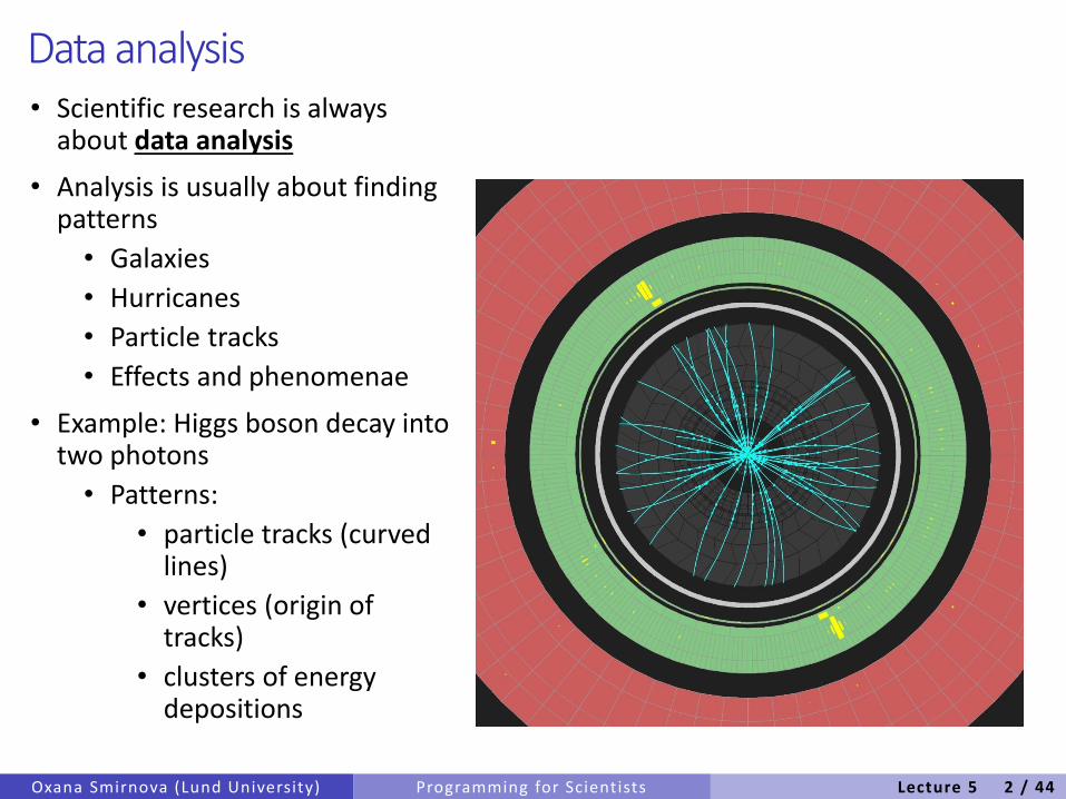
Data analysis• Scientific research is always

about data analysis

• Analysis is usually about finding patterns

• Galaxies

• Hurricanes

• Particle tracks

• Effects and phenomenae

• Example: Higgs boson decay into two photons

• Patterns:

• particle tracks (curved lines)

• vertices (origin of tracks)

• clusters of energy depositions


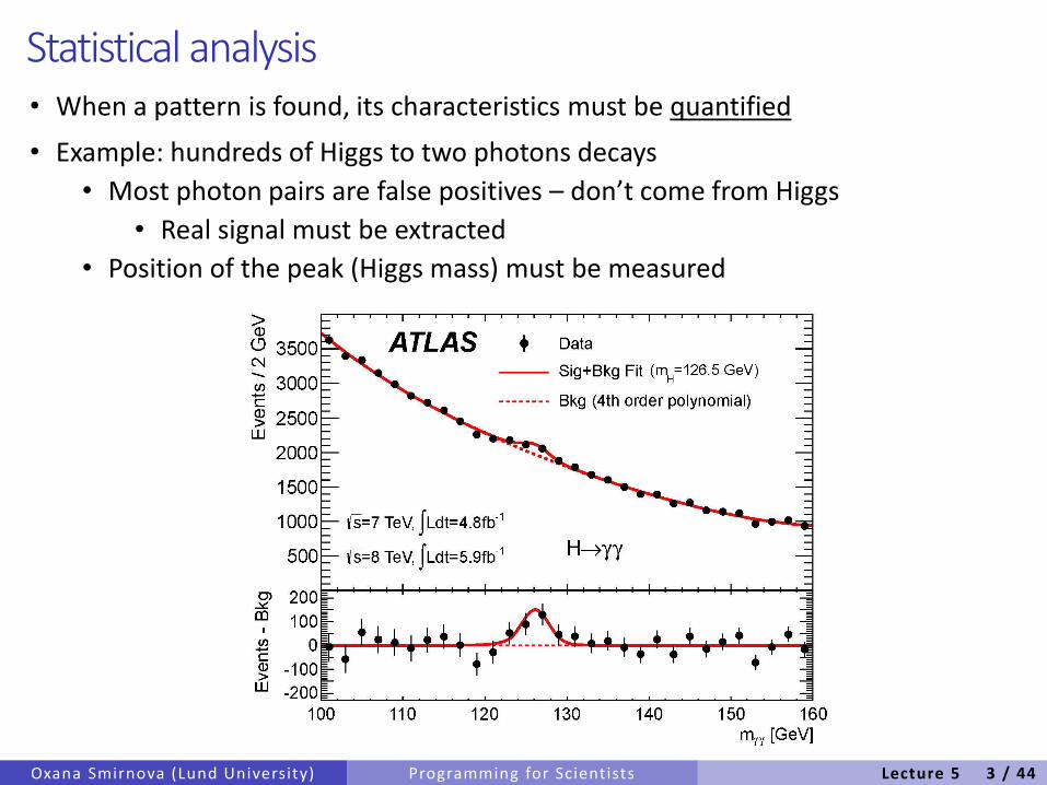
Statistical analysis• When a pattern is found, its characteristics must be quantified

• Example: hundreds of Higgs to two photons decays

• Most photon pairs are false positives – don’t come from Higgs

• Real signal must be extracted

• Position of the peak (Higgs mass) must be measured


Statistical methods• Statistics is used to analyze data that have probabilistic nature and/or have

random variations• Even several measurements of the same object with the same tool bring

varying results, so statistics is needed to deduce the measured value and standard deviation

• Statistic can be either descriptive (as in the example above), or inferential(hypothesis testing)

• Statistical methods are used to find patterns and to quantify the results• In the Higgs example, statistical analysis is used to, for example:

• Identify location of the signals left by particles• Reconstruct track patterns from detected signals• Reconstruct vertices from tracks• Assign energy and momentum to tracks• Quantify position and width of the observed peak• Test hypothesis that the observed peak is consistent with the Higgs

boson

• We need software tools to do all this analysis!


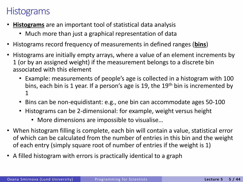
Histograms• Histograms are an important tool of statistical data analysis

• Much more than just a graphical representation of data

• Histograms record frequency of measurements in defined ranges (bins)

• Histograms are initially empty arrays, where a value of an element increments by 1 (or by an assigned weight) if the measurement belongs to a discrete bin associated with this element

• Example: measurements of people’s age is collected in a histogram with 100 bins, each bin is 1 year. If a person’s age is 19, the 19th bin is incremented by 1

• Bins can be non-equidistant: e.g., one bin can accommodate ages 50-100

• Histograms can be 2-dimensional: for example, weight versus height

• More dimensions are impossible to visualise…

• When histogram filling is complete, each bin will contain a value, statistical error of which can be calculated from the number of entries in this bin and the weight of each entry (simply square root of number of entries if the weight is 1)

• A filled histogram with errors is practically identical to a graph


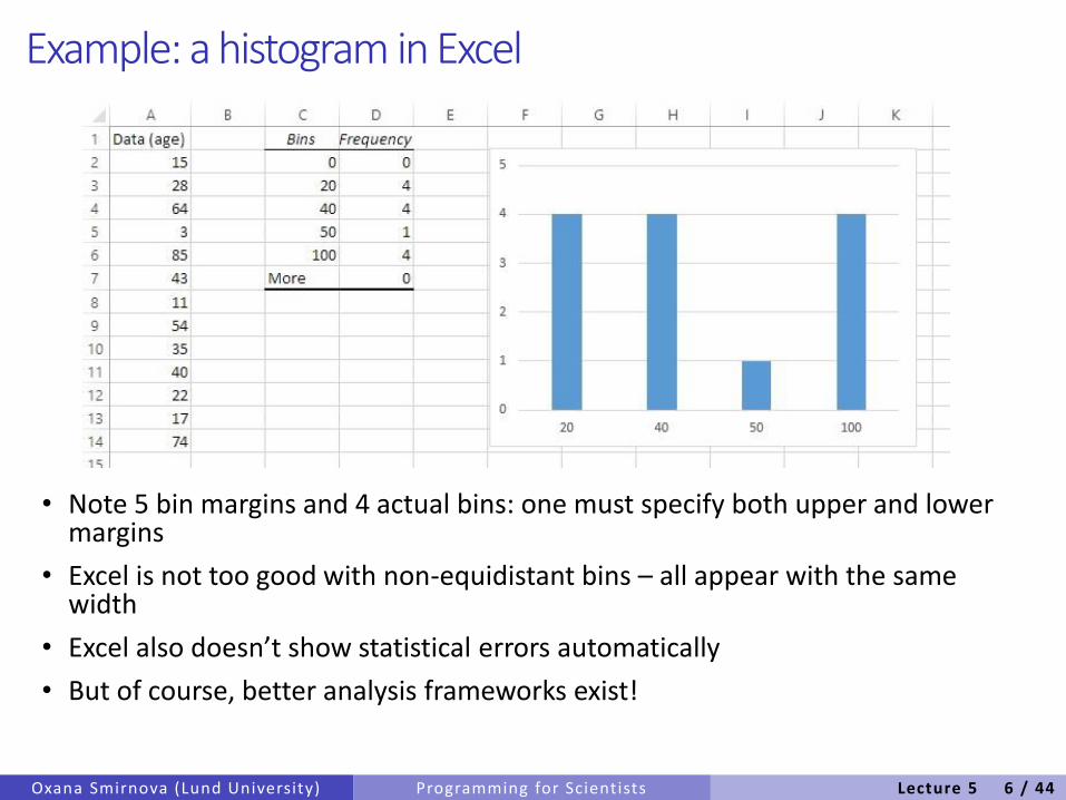
Example: a histogram in Excel

• Note 5 bin margins and 4 actual bins: one must specify both upper and lower margins

• Excel is not too good with non-equidistant bins – all appear with the same width

• Excel also doesn’t show statistical errors automatically

• But of course, better analysis frameworks exist!


Fitting histograms• Most measured distributions can be described by a theoretical function with

several parameters• Simplest: straight line, has 2 parameters: • Gaussian is another example, has 3 parameters:

• Finding values of the parameters (and their errors) is the main goal of many analyses

• The process of finding parameters that describe the data best is called fitting• When parameters are good, the theory fits the data

• Several standard fitting algorithms exist. General approach is:• With initial parameters, calculate data to function “distance”• Change parameters step by step in order to minimize the “distance”

• Algorithms of this minimization can be different• “Distance” depends on errors: with large errors, any function will fit• “Distance” can be estimated differently by different algorithms; most

commonly used is the chi-square per degree of freedom test• Degrees of freedom depend on number of data points and free

parameters:

Oxana Smirnova (Lund University) Programming for Scientists

23

22 2/)(

1)(PPx

ePxF

xPPxF 21)(

paramdata NNndf

Lecture 5 7 / 44

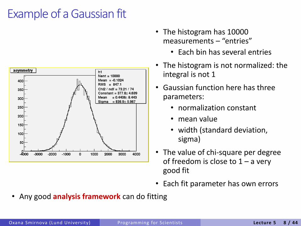
Example of a Gaussian fit• The histogram has 10000

measurements – “entries”

• Each bin has several entries

• The histogram is not normalized: the integral is not 1

• Gaussian function here has three parameters:

• normalization constant

• mean value

• width (standard deviation, sigma)

• The value of chi-square per degree of freedom is close to 1 – a very good fit

• Each fit parameter has own errors


• Any good analysis framework can do fitting

Lecture 5 8 / 44

Analysis frameworks and data formats• Frameworks hide complex details, providing simple utilities, tools and services

• Often the most complex detail to hide is the data format

• Data format in our context is a way of recording and organizing information• Binary or alphanumeric, possibly structured as tables, columns, raws or other

record units, order of records, links between records etc etc etc• There are almost as many data formats as there are researchers

• Some are even documented

• Different analysis frameworks are coupled to different data formats


Stri

p b

orr

ow

ed f

rom

Su

zan

ne

Pan

ace

ksl

ides

Lecture 5 9 / 44

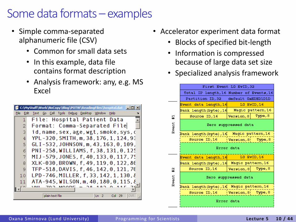
Some data formats –examples• Simple comma-separated

alphanumeric file (CSV)

• Common for small data sets

• In this example, data file contains format description

• Analysis framework: any, e.g. MS Excel

• Accelerator experiment data format

• Blocks of specified bit-length

• Information is compressed because of large data set size

• Specialized analysis framework


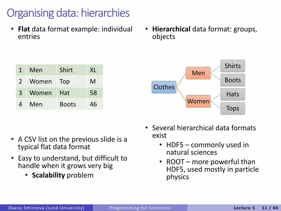
Organising data: hierarchies• Flat data format example: individual

entries

• A CSV list on the previous slide is a typical flat data format

• Easy to understand, but difficult to handle when it grows very big• Scalability problem

• Hierarchical data format: groups, objects

• Several hierarchical data formats exist• HDF5 – commonly used in

natural sciences• ROOT – more powerful than

HDF5, used mostly in particle physics


1 Men Shirt XL

2 Women Top M

3 Women Hat 58

4 Men Boots 46

Clothes

MenShirts

Boots

WomenHats

Tops

Lecture 5 11 / 44

ROOT –an object-oriented analysis framework• We will focus on ROOT – a specialized analysis framework developed at CERN

• Free and available for almost all platforms

• Relies on ROOT data format (a hierarchical database, actually)

• Has built-in C++ interpreter – you can use C++ in ROOT , like Python

• A complete ROOT tutorial normally takes several days; many such tutorials can be found on-line

• We will give a short introduction, re-using some official slides


What is ROOT?• The ROOT system is an object-oriented (OO) framework for large scale data

analysis (and even simulation)

• Written in C++

• Provides, among others,

• An efficient hierarchical OO database

• A C++ interpreter (CINT)

• Advanced statistical analysis (multi-dimensional histogramming, fitting, minimization and cluster finding algorithms)

• Visualization tools

• And much, much more

• The user interacts with ROOT via a graphical user interface, the commandline or scripts

• The command and scripting language is C++ (thanks to the embedded CINT C++ interpreter)

• Large scripts can be compiled and dynamically loaded


How to get and set up ROOT• ROOT is absolutely free and needs no licenses

• On Ubuntu, it is available from universe repositories

• Install package root-system

• Otherwise, go to http://root.cern.ch

and download what you need

• Currently recommended version is 5.xx

• Installation from source is for brave people: will take some time and may produce odd error messages

• You can configure your ROOT preferences using ~/.rootrc file

• There are also scripts rootlogon.C, rootlogoff.C (executed on logon and logoff) and rootalias.C (loaded on logon)

• History is saved in ~/.root_hist file

• Read ROOT documentation for details (or Google “ROOT getting started”)


http://root.cern.ch/

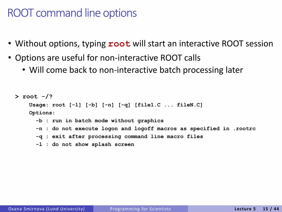
ROOT command line options

• Without options, typing root will start an interactive ROOT session

• Options are useful for non-interactive ROOT calls

• Will come back to non-interactive batch processing later

> root -/?

Usage: root [-l] [-b] [-n] [-q] [file1.C ... fileN.C]

Options:

-b : run in batch mode without graphics

-n : do not execute logon and logoff macros as specified in .rootrc

-q : exit after processing command line macro files

-l : do not show splash screen


Several ways to work with ROOT• Type root at the command line prompt

• This starts a new “shell” from which you can work with data by using C++ instructions and scripts

• One can also launch a ROOT GUI (see next slide)

• To exit, type .q

• To run a script (e.g. a tutorial), type .x <scriptname.C>

• To load functions from a file, type .L <scriptname.C>

• To execute a regular shell command, type .! <command>

• You can also link your code with the ROOT libraries and make the ROOT classes available in your own program

• the libraries are designed and organized to minimize dependencies

• Other relevant commands:

• rootcint – starts a utility to create a class dictionary for CINT. You will see how this utility is used is the section about adding your own class to ROOT.

• cint – a C++ interpreter that can be used independently of ROOT


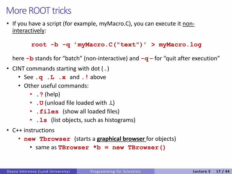
More ROOT tricks• If you have a script (for example, myMacro.C), you can execute it non-

interactively:

root -b -q ’myMacro.C("text")’ > myMacro.log

here -b stands for “batch” (non-interactive) and -q – for “quit after execution”

• CINT commands starting with dot (.)

• See .q .L .x and .! above

• Other useful commands:

• .? (help)

• .U (unload file loaded with .L)

• .files (show all loaded files)

• .ls (list objects, such as histograms)

• C++ instructions

• new Tbrowser (starts a graphical browser for objects)

• same as TBrowser *b = new TBrowser()


Built-in ROOT C and C++ interpreter: CINT• Main goal: provide a framework for C and C++ “scripting” – somewhat like

Python

• As a separate software, CINT code is available under an Open Source license

• It implements about 95% of ANSI C and 90% of ANSI C++

• It is robust and complete enough to interpret itself (90000 lines of C, 5000 lines of C++)

• Has good debugging facilities

• Has a byte code compiler

• In many cases it is faster than tcl, Perl and Python• Large scripts can still be compiled for optimal performance

• CINT is used in ROOT:• As command line interpreter• As script interpreter• To generate class dictionaries• To generate function/method calling stubs

• In ROOT, the command line, script and programming language become the same


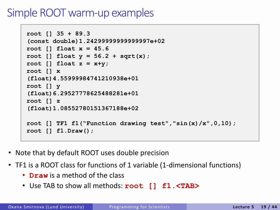
Simple ROOT warm-up examples

• Note that by default ROOT uses double precision

• TF1 is a ROOT class for functions of 1 variable (1-dimensional functions)

• Draw is a method of the class

• Use TAB to show all methods: root [] f1.<TAB>


root [] 35 + 89.3

(const double)1.24299999999999997e+02

root [] float x = 45.6

root [] float y = 56.2 + sqrt(x);

root [] float z = x+y;

root [] x

(float)4.55999984741210938e+01

root [] y

(float)6.29527778625488281e+01

root [] z

(float)1.08552780151367188e+02

root [] TF1 f1(“Function drawing test","sin(x)/x",0,10);

root [] f1.Draw();

Lecture 5 19 / 44

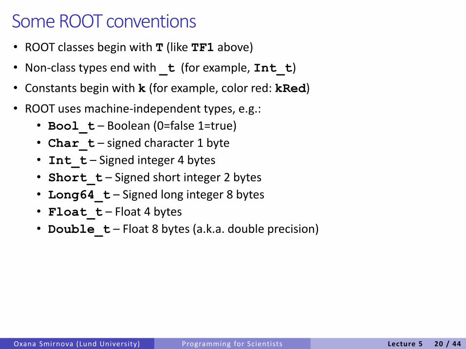
Some ROOT conventions• ROOT classes begin with T (like TF1 above)

• Non-class types end with _t (for example, Int_t)

• Constants begin with k (for example, color red: kRed)

• ROOT uses machine-independent types, e.g.:

• Bool_t – Boolean (0=false 1=true)

• Char_t – signed character 1 byte

• Int_t – Signed integer 4 bytes

• Short_t – Signed short integer 2 bytes

• Long64_t – Signed long integer 8 bytes

• Float_t – Float 4 bytes

• Double_t – Float 8 bytes (a.k.a. double precision)


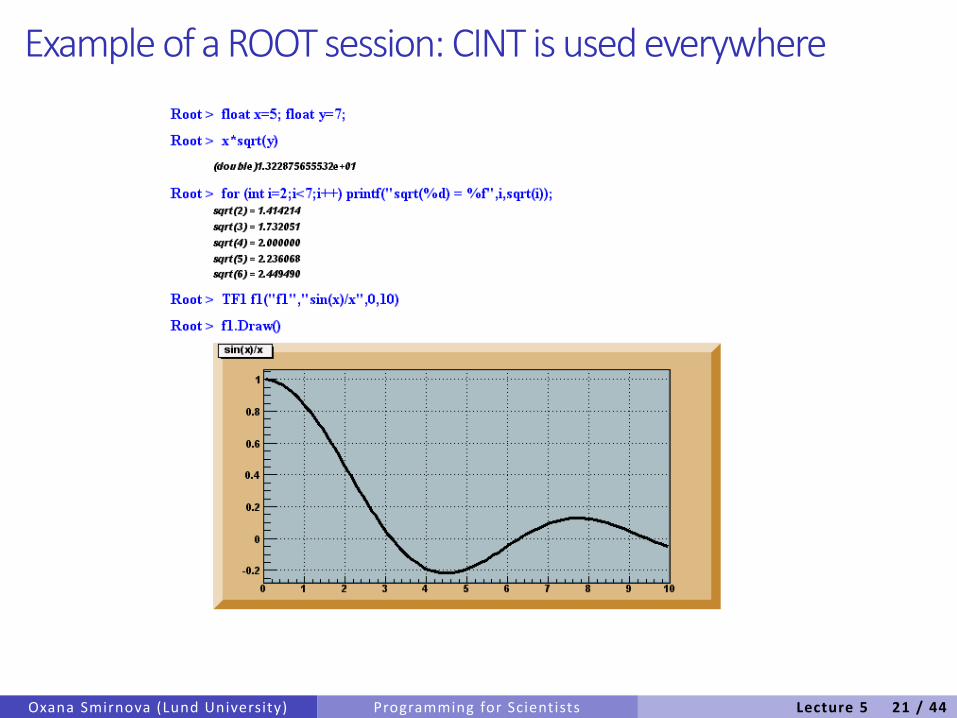
Example of a ROOT session: CINT is used everywhere


Scripts in ROOT• Un-named Script: a simple short-cut (like a bash script)

• Starts with { and ends with }

• All variables are in the global scope

• No class definitions

• No function declarations

• No parameters

• Named Script: essentially, a C++ program

• C++ functions

• Scope rules follow standard C++

• Function with the same name as the file is executed with a .x

• Parameters

• Class definitions (derived from a compiled class at your own risk)


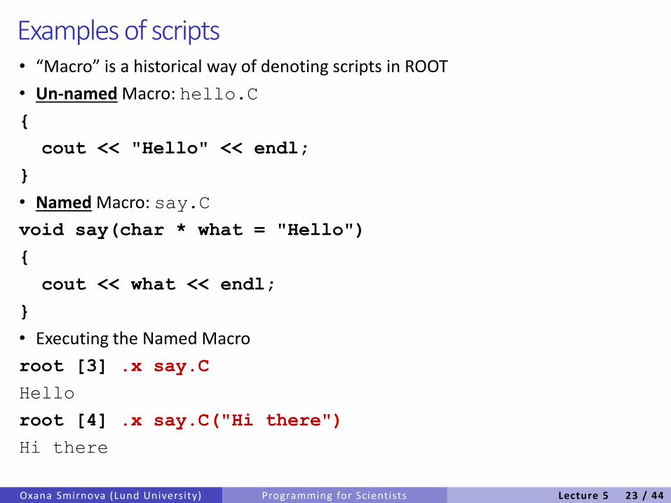
Examples of scripts• “Macro” is a historical way of denoting scripts in ROOT

• Un-named Macro: hello.C

{

cout << "Hello" << endl;

}

• Named Macro: say.C

void say(char * what = "Hello")

{

cout << what << endl;

}

• Executing the Named Macro

root [3] .x say.C

Hello

root [4] .x say.C("Hi there")

Hi there


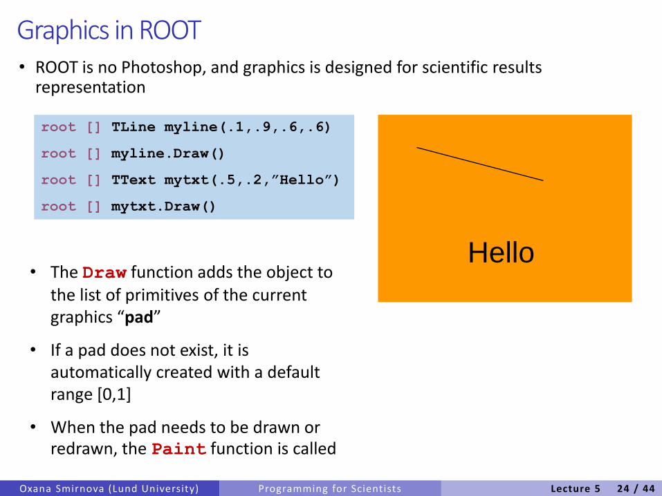
Graphics in ROOT• ROOT is no Photoshop, and graphics is designed for scientific results

representation


Hello

root [] TLine myline(.1,.9,.6,.6)

root [] myline.Draw()

root [] TText mytxt(.5,.2,”Hello”)

root [] mytxt.Draw()

• The Draw function adds the object to the list of primitives of the current graphics “pad”

• If a pad does not exist, it is automatically created with a default range [0,1]

• When the pad needs to be drawn or redrawn, the Paint function is called

Lecture 5 24 / 44

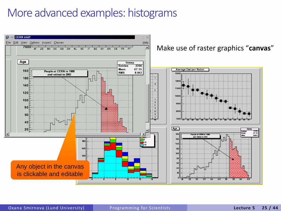
More advanced examples: histograms


Make use of raster graphics “canvas”

Any object in the canvas

is clickable and editable

Lecture 5 25 / 44

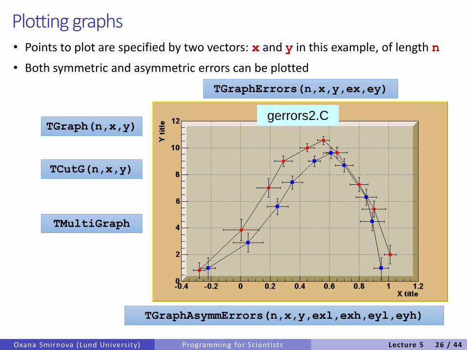
Plotting graphs• Points to plot are specified by two vectors: x and y in this example, of length n

• Both symmetric and asymmetric errors can be plotted


TGraph(n,x,y)

TCutG(n,x,y)

TGraphErrors(n,x,y,ex,ey)

TGraphAsymmErrors(n,x,y,exl,exh,eyl,eyh)

TMultiGraph

gerrors2.C

Lecture 5 26 / 44

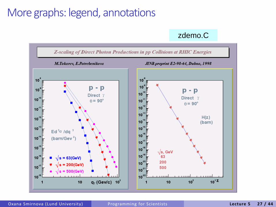
More graphs: legend, annotations


zdemo.C

Lecture 5 27 / 44

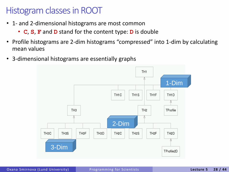
Histogram classes in ROOT


• 1- and 2-dimensional histograms are most common

• C, S, F and D stand for the content type: D is double

• Profile histograms are 2-dim histograms “compressed” into 1-dim by calculating mean values

• 3-dimensional histograms are essentially graphs

1-Dim

2-Dim

3-Dim

Lecture 5 28 / 44

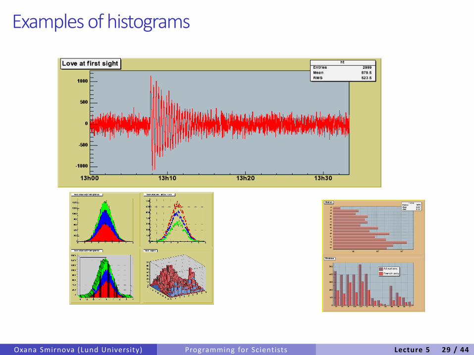
Examples of histograms


Fitting in ROOT• Histograms can be fitted with any function via TH1::Fit. Two fitting

algorithms are supported: Chi-square method and Log Likelihood

• The user functions may be of the following types:• standard functions: gaus, landau, expo, poln• combination of standard functions; poln + gaus

• A C++ interpreted function or a C++ precompiled function

• An option is provided to compute the integral of the function bin by bin instead of simply compute the function value at the center of the bin.

• When an histogram is fitted, the resulting function with its parameters is added to the list of functions of this histogram. If the histogram is made persistent (saved as a file), the list of associated functions is also persistent.

• One can retrieve the function/fit parameters with calls such as:• Double_t chi2 = myfunc->GetChisquare();

• Double_t par0 = myfunc->GetParameter(0); //value of 1st parameter

• Double_t err0 = myfunc->GetParError(0); //error on first parameter


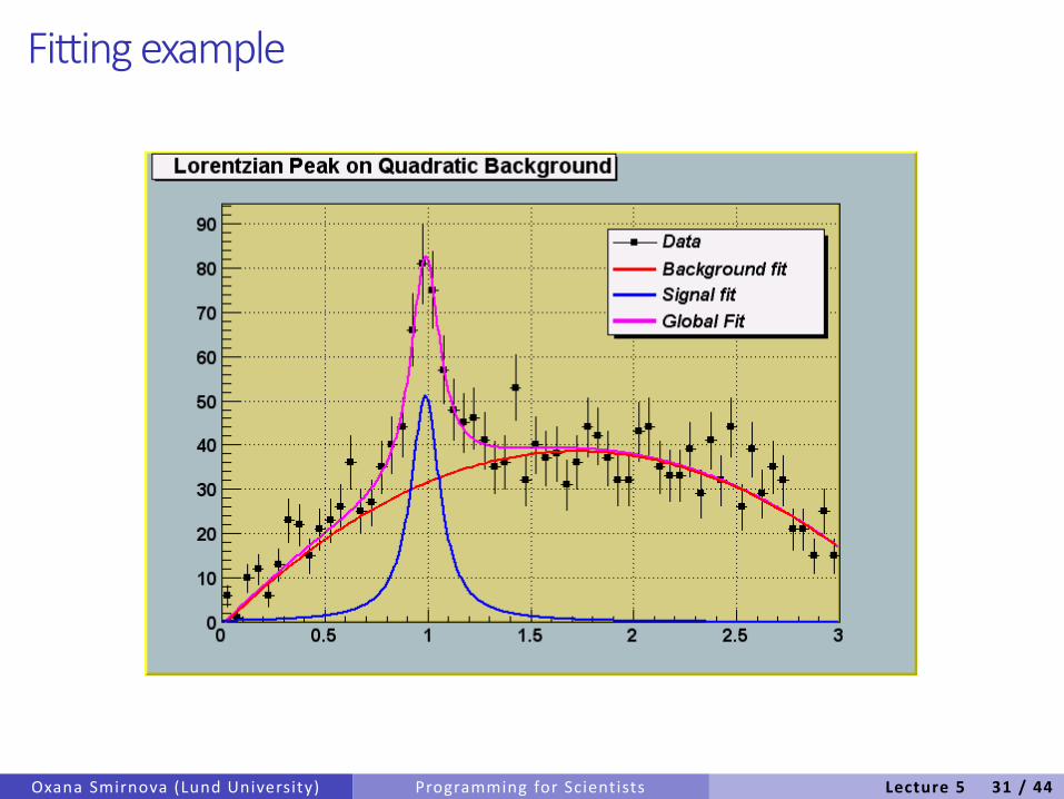
Fitting example


Random numbers and histograms• TH1::FillRandom can be used to randomly fill an histogram using either of:

• the contents of an existing TF1 analytic function

• another histogram

• Example: the following two statements create and fill an histogram 10000 times with a default Gaussian distribution of mean 0 and sigma 1:

TH1F h1("h1","histo from a gaussian",100,-3,3);

h1.FillRandom("gaus",10000);

• TH1::GetRandom can be used to return a random number distributed according the contents of an histogram


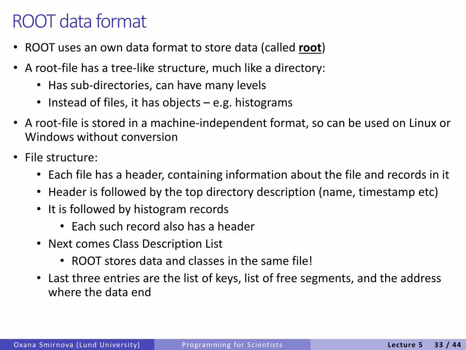
ROOT data format• ROOT uses an own data format to store data (called root)

• A root-file has a tree-like structure, much like a directory:

• Has sub-directories, can have many levels

• Instead of files, it has objects – e.g. histograms

• A root-file is stored in a machine-independent format, so can be used on Linux or Windows without conversion

• File structure:

• Each file has a header, containing information about the file and records in it

• Header is followed by the top directory description (name, timestamp etc)

• It is followed by histogram records

• Each such record also has a header

• Next comes Class Description List

• ROOT stores data and classes in the same file!

• Last three entries are the list of keys, list of free segments, and the address where the data end


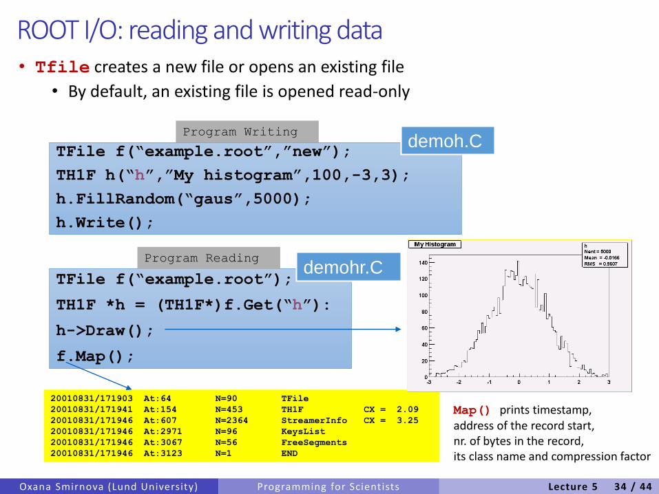
ROOT I/O: reading and writing data• Tfile creates a new file or opens an existing file

• By default, an existing file is opened read-only


TFile f(“example.root”,”new”);

TH1F h(“h”,”My histogram”,100,-3,3);

h.FillRandom(“gaus”,5000);

h.Write();

TFile f(“example.root”);

TH1F *h = (TH1F*)f.Get(“h”):

h->Draw();

f.Map();

Program Writing

Program Reading

20010831/171903 At:64 N=90 TFile

20010831/171941 At:154 N=453 TH1F CX = 2.09

20010831/171946 At:607 N=2364 StreamerInfo CX = 3.25

20010831/171946 At:2971 N=96 KeysList

20010831/171946 At:3067 N=56 FreeSegments

20010831/171946 At:3123 N=1 END

demoh.C

demohr.C

Map() prints timestamp, address of the record start, nr. of bytes in the record,its class name and compression factor

Lecture 5 34 / 44

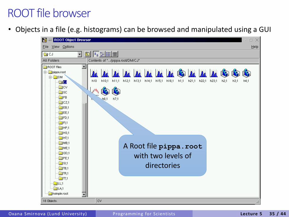
ROOT file browser• Objects in a file (e.g. histograms) can be browsed and manipulated using a GUI


A Root file pippa.rootwith two levels of

directories

Lecture 5 35 / 44

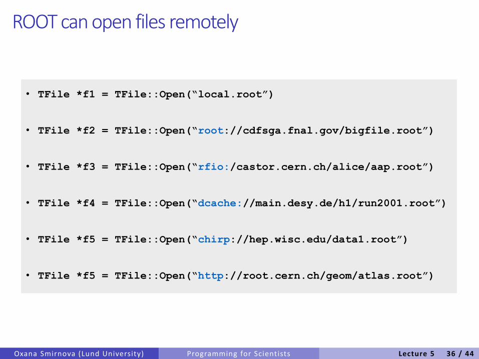
ROOT can open files remotely


• TFile *f1 = TFile::Open(“local.root”)

• TFile *f2 = TFile::Open(“root://cdfsga.fnal.gov/bigfile.root”)

• TFile *f3 = TFile::Open(“rfio:/castor.cern.ch/alice/aap.root”)

• TFile *f4 = TFile::Open(“dcache://main.desy.de/h1/run2001.root”)

• TFile *f5 = TFile::Open(“chirp://hep.wisc.edu/data1.root”)

• TFile *f5 = TFile::Open(“http://root.cern.ch/geom/atlas.root”)

Lecture 5 36 / 44

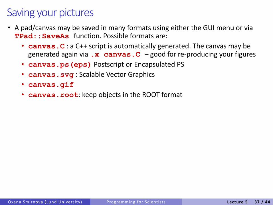
Saving your pictures• A pad/canvas may be saved in many formats using either the GUI menu or via TPad::SaveAs function. Possible formats are:

• canvas.C : a C++ script is automatically generated. The canvas may be generated again via .x canvas.C – good for re-producing your figures

• canvas.ps(eps) Postscript or Encapsulated PS

• canvas.svg : Scalable Vector Graphics

• canvas.gif

• canvas.root: keep objects in the ROOT format


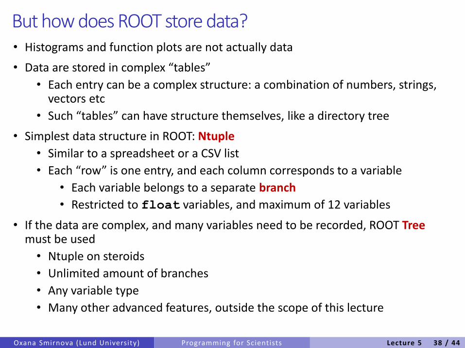
But how does ROOT store data?• Histograms and function plots are not actually data

• Data are stored in complex “tables”

• Each entry can be a complex structure: a combination of numbers, strings, vectors etc

• Such “tables” can have structure themselves, like a directory tree

• Simplest data structure in ROOT: Ntuple

• Similar to a spreadsheet or a CSV list

• Each “row” is one entry, and each column corresponds to a variable

• Each variable belongs to a separate branch

• Restricted to float variables, and maximum of 12 variables

• If the data are complex, and many variables need to be recorded, ROOT Treemust be used

• Ntuple on steroids

• Unlimited amount of branches

• Any variable type

• Many other advanced features, outside the scope of this lecture


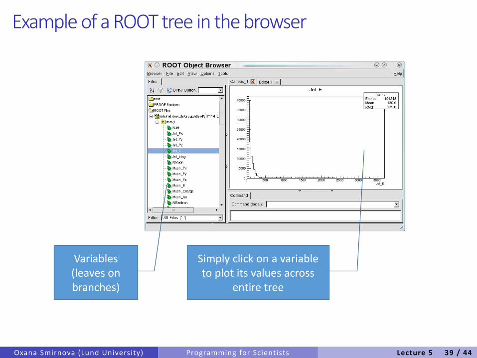
Example of a ROOT tree in the browser


Variables(leaves on branches)

Simply click on a variable to plot its values across

entire tree

Lecture 5 39 / 44

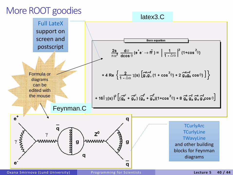
More ROOT goodies


Full LateXsupport on screen and postscript

TCurlyArcTCurlyLineTWavyLine

and other building blocks for Feynman

diagrams

Formula or diagramscan be

edited with

the mouse

Feynman.C

latex3.C

Lecture 5 40 / 44

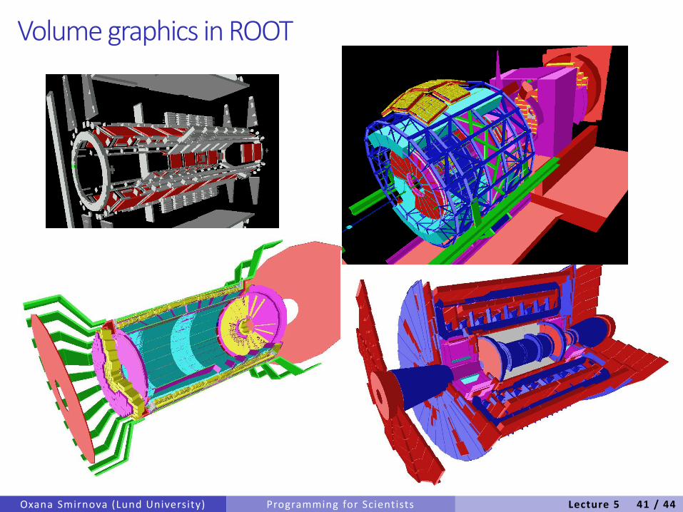
Volume graphics in ROOT


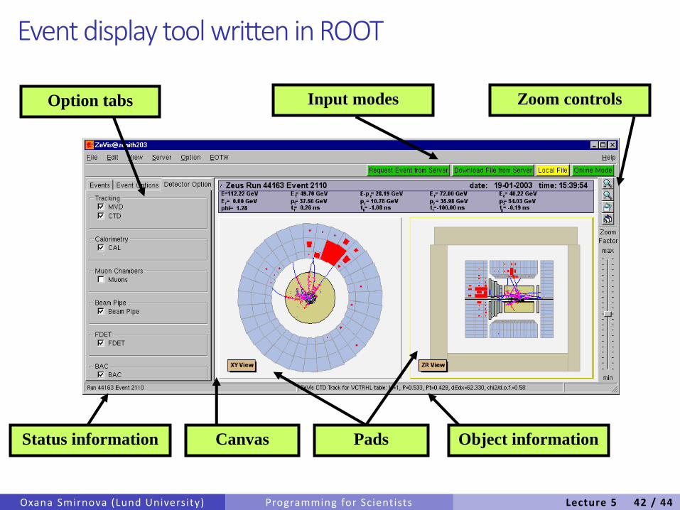
Event display tool written in ROOT


Option tabs

Status information Canvas Pads Object information

Input modes Zoom controls

Lecture 5 42 / 44

Summary of ROOT services and utilities• Histogramming and Fitting

• Graphics (2D, 3D)

• Input/Output to file or socket: specialized for histograms, Ntuples (Trees)

• Collection Classes and Run Time Type Identification

• User Interface

• GUI: Browsers, Panels, Tree Viewer

• Command Line interface: C++ interpreter CINT

• Script Processor (C++ compiled ↔ C++ interpreted


A little bit extra: ROOT library structure• ROOT libraries are a layered structure

• The CORE classes are always required (support for RTTI, basic I/O and interpreter)

• The optional libraries (you load only what you use) Separation between data objects and the high level classes acting on these objects. Example, a batch job uses only the histogram library, no need to link histogram painter library.

• Shared libraries reduce the application link time

• Shared libraries reduce the application size

• ROOT shared libraries can be used with other class libraries


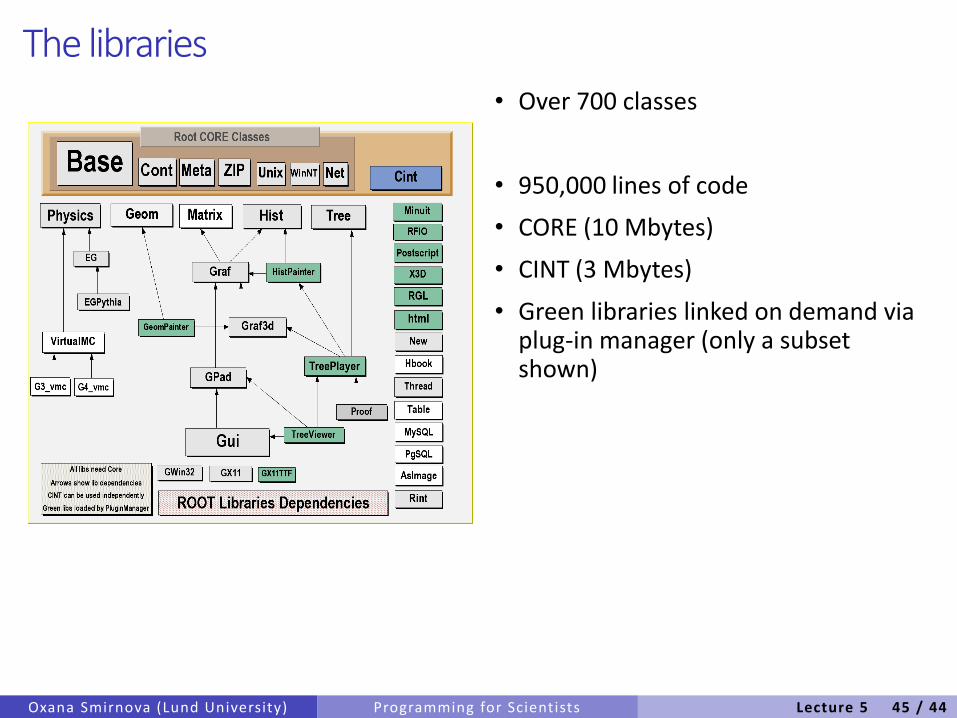
The libraries• Over 700 classes

• 950,000 lines of code

• CORE (10 Mbytes)

• CINT (3 Mbytes)

• Green libraries linked on demand via plug-in manager (only a subset shown)


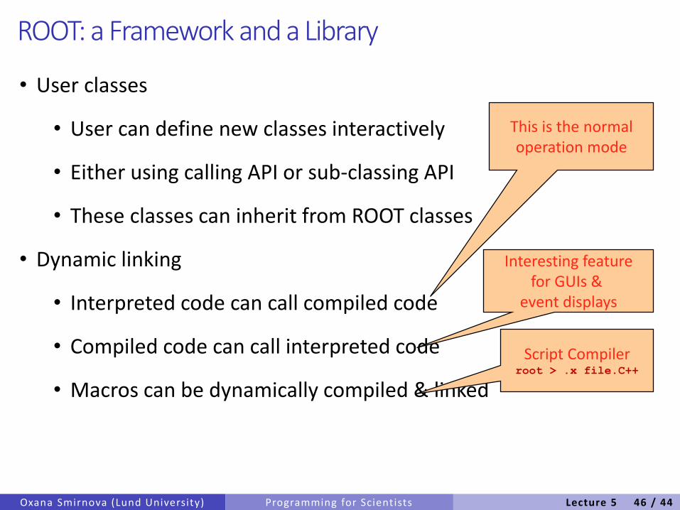
ROOT: a Framework and a Library

• User classes

• User can define new classes interactively

• Either using calling API or sub-classing API

• These classes can inherit from ROOT classes

• Dynamic linking

• Interpreted code can call compiled code

• Compiled code can call interpreted code

• Macros can be dynamically compiled & linked


This is the normaloperation mode

Interesting featurefor GUIs &

event displays

Script Compilerroot > .x file.C++

Lecture 5 46 / 44

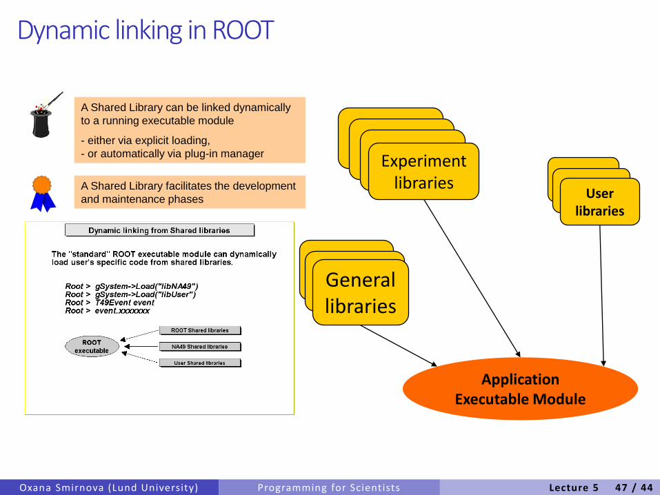
Dynamic linking in ROOT


ApplicationExecutable Module

Experimentlibraries

Userlibraries

Generallibraries

A Shared Library can be linked dynamically

to a running executable module

- either via explicit loading,

- or automatically via plug-in manager

A Shared Library facilitates the development

and maintenance phases

Lecture 5 47 / 44

Introduction to Programming and Computing for Scientists · Introduction to Programming and...

Documents

Transcript of Introduction to Programming and Computing for Scientists · Introduction to Programming and...