11

INTRODUCTION TO NEURAL COMPUTING • Knowledge resides in the weights or 'connections'

ijw between nodes (hence the older name for neural computing, 'connectionism'). The net’s weights are equivalent in biological terms to synaptic efficiencies though they are allowed to change their values in a less restricted way than their biological counterparts.

• The representation of this knowledge is distributed: each concept stored by the net corresponds to a pattern of activity over all nodes so that in turn each node is involved in representing many concepts.

• The weights are learned through experience, in a usually iterative procedure using an update rule for the change in the weight ijwΔ .

3 classes of learning: 1. SUPERVISED Information from a 'teacher' is provided that tells the net the output required for a given input. Weights are adjusted so as to minimise the difference between the desired and actual outputs for each input pattern. 2. REINFORCED The network receives a global reward/penalty signal (a lower quality of instructional information than in the supervised case). The weights are changed so as to develop an I/O behaviour that maximises the probability of receiving a reward and minimises that of receiving a penalty. If supervised training is 'learning with a teacher,' reinforcement training is 'learning with a critic.' 3. UNSUPERVISED The network is able to discover statistical regularities in its input data space and automatically develops different modes of behaviour to represent different classes of inputs (in practice some 'labelling' is usually required after training since it is not known beforehand which mode of behaviour will become associated with a given class).

12

A net’s architecture is the basic way that neurons are connected (without considering the strengths and signs of such connections). The architecture strongly determines what kinds of functions can be carried out, as weight-modifying algorithms normally only adjust the effects of connections, they do not usually add or subtract neurons or create/delete connections. Most neural networks currently used are of the feedforward type. These are arranged in layers such that information flows in a single direction, usually only from layer n to layer n+1 (ie can’t skip over layers such as connection layer 1 directly to layer 3). (Note the convention that an 'N-layer net' is one in which there are N layers of processing units, and an initial layer 0 that is a buffer to store the currently-seen pattern and which serves only to distribute inputs, not to carry out any computation; hence the above is, indeed, a '2-layer net.') The input to the net in layer 0 is passed forward layer by layer, each layer’s neuron units performing some computation before handing information on the to next layer. By the use of adaptive interconnects ('weights') the net learns to perform a set of mappings from input vectors x to output vectors y.

13

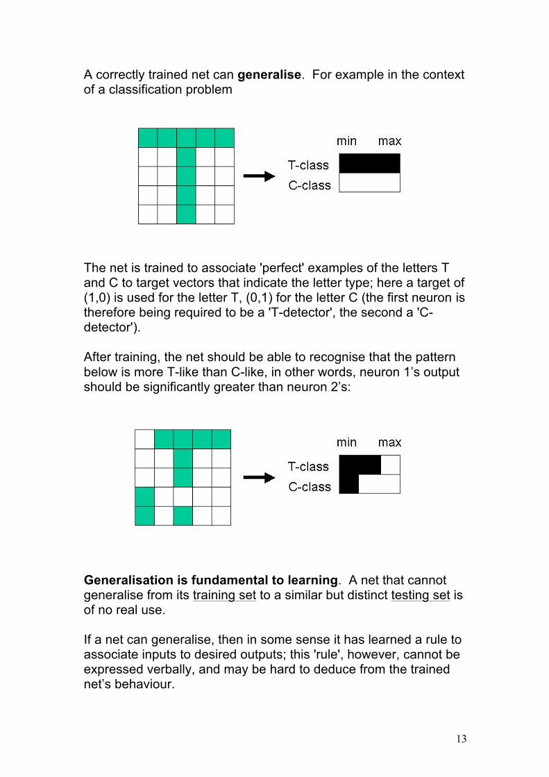
A correctly trained net can generalise. For example in the context of a classification problem The net is trained to associate 'perfect' examples of the letters T and C to target vectors that indicate the letter type; here a target of (1,0) is used for the letter T, (0,1) for the letter C (the first neuron is therefore being required to be a 'T-detector', the second a 'C-detector'). After training, the net should be able to recognise that the pattern below is more T-like than C-like, in other words, neuron 1’s output should be significantly greater than neuron 2’s: Generalisation is fundamental to learning. A net that cannot generalise from its training set to a similar but distinct testing set is of no real use. If a net can generalise, then in some sense it has learned a rule to associate inputs to desired outputs; this 'rule', however, cannot be expressed verbally, and may be hard to deduce from the trained net’s behaviour.

14

Applications of neural networks Neural computing, for reasons explained in the Introduction to this section of the course, is presently restricted to pattern matching, classification, and prediction tasks that do not require elaborate goal structures to be set up. While we might like to be able to develop neural networks that could be used, say, for autonomous robot guidance (and NASA/JPL for example have done a lot of research in this area) this will probably remain out of reach until we know more about the neural mechanisms that underlie cognition in real brains. The most successful current applications of neural computing generally satisfy the criteria:

• The task is well-defined -- we know precisely what we want (eg to classify on-camera images of faces into ‘employee’ or ‘intruder’; to predict future values of exchange rates based on their past values).

• There is a sufficient amount of data available to train the net

to acquire a useful function based on what it should have done in these past examples.

• The problem is not of the type for which a rule base could be

constructed, and which therefore could more easily be solved using a symbolic AI approach.

There are many situations in business and finance which satisfy these criteria, and this area is probably the one in which neural networks have been used most widely so far, and with a great deal of success.

15

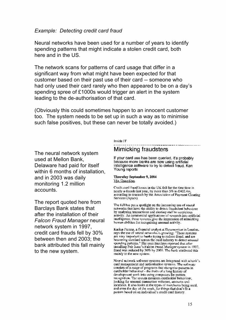
Example: Detecting credit card fraud Neural networks have been used for a number of years to identify spending patterns that might indicate a stolen credit card, both here and in the US. The network scans for patterns of card usage that differ in a significant way from what might have been expected for that customer based on their past use of their card -- someone who had only used their card rarely who then appeared to be on a day’s spending spree of £1000s would trigger an alert in the system leading to the de-authorisation of that card. (Obviously this could sometimes happen to an innocent customer too. The system needs to be set up in such a way as to minimise such false positives, but these can never be totally avoided.) The neural network system used at Mellon Bank, Delaware had paid for itself within 6 months of installation, and in 2003 was daily monitoring 1.2 million accounts. The report quoted here from Barclays Bank states that after the installation of their Falcon Fraud Manager neural network system in 1997, credit card frauds fell by 30% between then and 2003; the bank attributed this fall mainly to the new system.

16

Example: Predicting cash machine usage Banks want to keep cash machines filled, to keep their customers happy, but not to overfill them. Different cash machines will get different amounts of use, and a neural network can look at patterns of past withdrawals in order to decide how often, and with how much cash, a given machine should be refilled. Siemens developed a very successful neural network system for this task; in benchmark tests in 2004 it easily outperformed all its rival (including non-neural) predictor systems, and, as reported below, could gain a bank very significant additional profit from funds that would otherwise be tied up in cash machines.

17

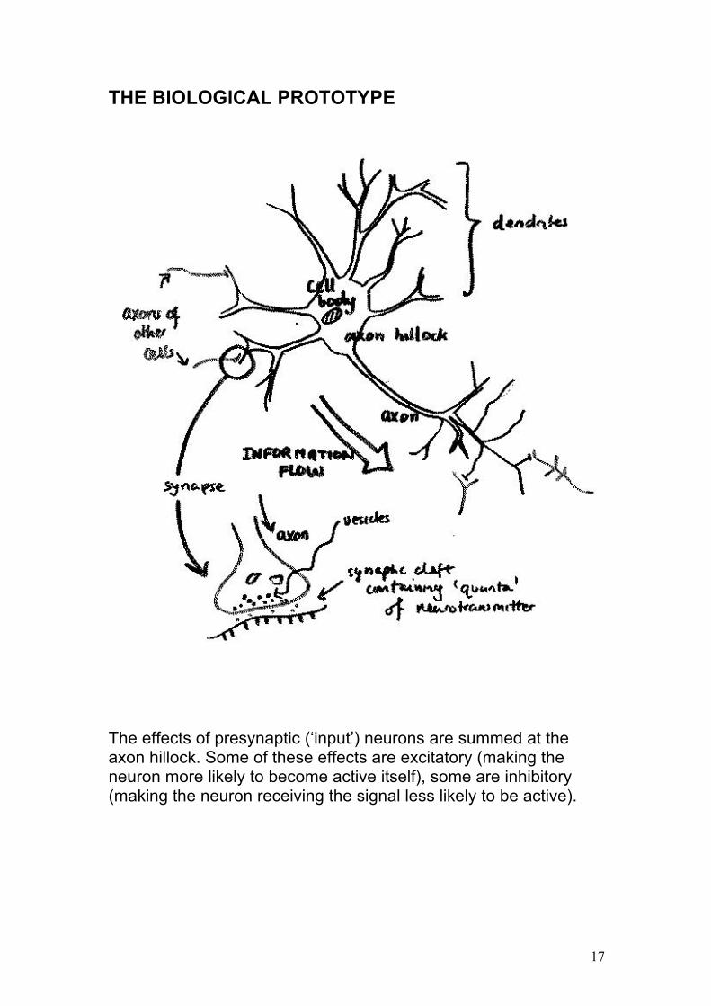
THE BIOLOGICAL PROTOTYPE

The effects of presynaptic (‘input’) neurons are summed at the axon hillock. Some of these effects are excitatory (making the neuron more likely to become active itself), some are inhibitory (making the neuron receiving the signal less likely to be active).

18

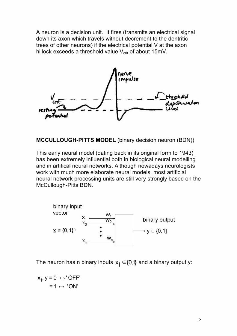
A neuron is a decision unit. It fires (transmits an electrical signal down its axon which travels without decrement to the dentritic trees of other neurons) if the electrical potential V at the axon hillock exceeds a threshold value Vcrit of about 15mV.

MCCULLOUGH-PITTS MODEL (binary decision neuron (BDN)) This early neural model (dating back in its original form to 1943) has been extremely influential both in biological neural modelling and in artifical neural networks. Although nowadays neurologists work with much more elaborate neural models, most artificial neural network processing units are still very strongly based on the McCullough-Pitts BDN. The neuron has n binary inputs }1,0{xj∈ and a binary output y:

'ON' 1= 'OFF ' 0=y ,x j

↔↔

19

Each input signal jx is multiplied by a weight jw which is effectively the synaptic strength in this model.

0<w j ↔ input j has an inhibitory effect ↔ 0>w j input j has an excitatory effect

The weighted signals are summed, and this sum is then compared to a threshold s:

!

y = 0 if w jx jj=1

n

" # s

!

y = 1 if w jx jj=1

n

" > s

This can equivalently be written as

!

y = " wjx jj=1

n

# - s$

% & &

'

( ) )

where ( ) xθ is the step (or Heaviside) function It can also be useful to write this as ( ) aθ=y with the activation a defined as

!

a = wjx jj=1

n

" - s

as this separates the roles of the BDN activation function (whose linear form is still shared by almost all common neural network models) and the firing function θ(a), the step form of which has since been replaced by an alternative, smoother form in more computationally powerful modern neural network models.

20

THE PERCEPTRON MODEL (Rosenblatt, 1957)

• USES BDN NODES • CLASSIFIES PATTERNS THROUGH SUPERVISED

LEARNING. • FEEDFORWARD ARCHITECTURE -- BUT ONLY OUTPUT

LAYER HAS ADAPTIVE WEIGHTS. • THERE IS A PROOF THAT THE PERCEPTRON TRAINING

ALGORITHM WILL ALWAYS CONVERGE TO A CORRECT SOLUTION -- PROVIDED THAT SUCH A FUNCTION CAN IN PRINCIPLE BE LEARNED BY A SINGLE-LAYER NET.

This 4-input, 3-output perceptron net could be used to classify four-component patterns into one of three types, symbolised by the target output values (1,0,0) (Type 1); (0,1,0) (Type 2); (0,0,1) (Type 3).

21

Perceptron processing unit This is essentially a binary decision neuron (BDN), in which the threshold for each neuron is treated as an extra weight w0 from an imagined unit, the bias unit, which is always 'on' (x0=1):

!

y = " w jx jj=1

n

# - s$

% & &

'

( ) ) = " wjx j

j=0

n

#$

% & &

'

( ) ) if w0 = -s

This notational change from the McCullough-Pitts BDN formulation was made for two reasons:

1. To emphasise that in the perceptron, threshold values are adaptive, unlike those of biological neurons, which correspond to a fixed voltage level that has to be exceeded before a neuron can fire. Using a notation that represents the effect of the threshold as that of another weight highlights this difference.

2. For compactness of expression in the learning rules -- we do

not now need two separate rules, one for the weights 1..nj ,wΔ j = and one for the adaptive threshold sΔ , just one

for this extended set of weights 0..nj ,wΔ j = .

Perceptron learning algorithm Each of the i=1..N n-input (in the example on the previous page N=3, n=4) BDNs in the net is required to map one set of input vectors n}1,0{∈ (CLASS A) to 1, and another set (CLASS B) to 0:

Bx if 0Ax if 1

{=tp

pp,i ∈

∈

p,it is the desired response for neuron i to input pattern px . The

learning rule is supervised because p,it is known for all patterns p = 1..P (where P is the total number of patterns in the training set).

22

Outline of the algorithm:

• initialise: for each node i in the net, set ijw , j=0..n to their initial values.

• repeat

for p =1 to P

o load pattern px , and note desired outputs p,it .

o calculate node outputs for this pattern according to

!

yi,p = " wijx j,pj=0

n

#$

% & &

'

( ) )

o adapt weights

p,jp,ip,iijij x)y-t(ηww +→ until (error = 0) or (max epochs reached) Notes

• Using this procedure, any ijw can change its value from positive (excitatory) to negative (inhibitory), regardless of the origin of the input signal with which this weight is associated. This cannot happen in biological neural nets, where a neurons’s chemical signal (neurotransmitter) is either of an excitatory or inhibitory type, so that, say, if j is an excitatory neuron, all ijw must be 'excitatory synaptic weights' (in the BDN formulation, greater than 0). However this restriction, known as Dale’s Law, is an instance where it would not be desirable to follow the guidelines of biology too closely -- the restriction has no innate value, it is just an artifact of how real neurons work and its introduction would only reduce the flexibility of artifical neural networks.

23

• Small initial values for the weights, both positive and negative -- for example in the interval ]1.0,1.0[ +− -- give the smoothest convergence to a solution, but in fact for this type of net any initial set will eventually reach a solution -- if one is possible.

• The weight-change rule ijijij wΔww +→ , where

p,jp,ip,iij x)y-t(η=wΔ is known as the Widrow-Hoff delta rule (Bernard Widrow was another early pioneer of neural computing, marketing a rival system to Rosenblatt’s perceptron known as the 'Adeline' or 'Madeline.')

• A single epoch is a complete presentation of all P patterns,

together with any weight updates necessary (ie everything between 'repeat' and 'until').

• η (always positive) is the training rate. The original

perceptron algorithm used η=1. Smaller values make for smoother convergence, but as with the case of starting weight values above, no choice will actually cause the net to fail unless the problem is fundamentally insoluble by a perceptron net. (This kind of robustness is NOT typical of neural network training algorithms in general!)

Error function This is usually defined by the mean squared error

!

E =1

PN (ti,p - yi,p )2

i=1

N

"p=1

P

"

(where P is the number of training patterns, N the number of output nodes) or the root mean squared (rms) error E=Erms Of these the rms error is the one most frequently used as it gives some feel for the 'average difference' between desired and actual outputs. The mean squared error itself can be rather deceiving as this sum of squared-fractional values can appear to have fallen very significantly with epoch even though the net has some substantial amount of learning still to do.

24

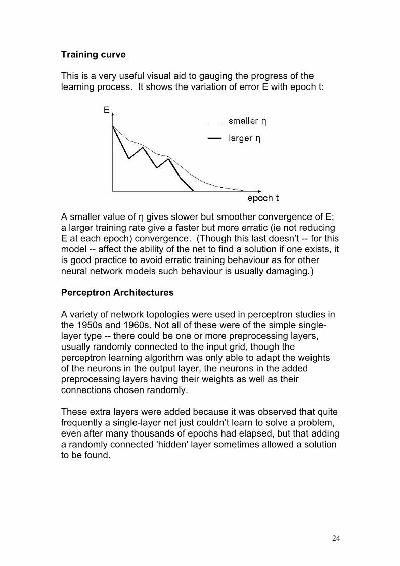
Training curve This is a very useful visual aid to gauging the progress of the learning process. It shows the variation of error E with epoch t: A smaller value of η gives slower but smoother convergence of E; a larger training rate give a faster but more erratic (ie not reducing E at each epoch) convergence. (Though this last doesn’t -- for this model -- affect the ability of the net to find a solution if one exists, it is good practice to avoid erratic training behaviour as for other neural network models such behaviour is usually damaging.) Perceptron Architectures A variety of network topologies were used in perceptron studies in the 1950s and 1960s. Not all of these were of the simple single-layer type -- there could be one or more preprocessing layers, usually randomly connected to the input grid, though the perceptron learning algorithm was only able to adapt the weights of the neurons in the output layer, the neurons in the added preprocessing layers having their weights as well as their connections chosen randomly. These extra layers were added because it was observed that quite frequently a single-layer net just couldn’t learn to solve a problem, even after many thousands of epochs had elapsed, but that adding a randomly connected 'hidden' layer sometimes allowed a solution to be found.

25

2-layer perceptron character classifier However it wasn’t fully appreciated that

• It was the restriction to a single learning layer (it’s being impossible to use the Widrow-Hoff rule on any but output layer neurons, as it’s only for these neurons that target values are defined) that was the fundamental reason for the failures.

• The trial-and-error connection of a preprocessing layer, reconnecting if learning still failed, was in effect a primitive form of training for this hidden layer (a random search in connection and weight space).

Limitations of perceptrons (Minsky and Papert, 1969) As described above, there were some desired pattern classifications for which the perceptron training algorithm failed to converge to zero error, and Minsky and Papert deduced that these were when the individual neurons were being required to perform functions of a certain mathematical type, known as non-linearly separable functions.

26

This might not have mattered if the proportion of such functions was small, but unfortunately as the number of inputs to a single BDN neuron grows, the proportion of those functions which might be required to be developed by a net with a single learning layer, but are not representable by a BDN neuron, grows extremely fast (or conversely, the number which can be performed, those which are linearly separable) drops equivalently quickly: n Number of

Possible functions Number of linearly separable functions

Proportion of linearly separable functions

1 4 4 1 2 16 14 0.88 3 256 104 0.41 4 65,336 1,882 0.03 5 ~4.3x109 94,572 ~2.2x10-5 6 ~1.8x1019 5,028,134 ~2.8x10-13

It’s not surprising therefore that Rosenblatt’s group frequently encountered difficulties when using their perceptron nets for image recognition problems. However remember they were able to partly overcome these difficulties with a trial-and-error training method involving a 'preprocessing layer.' It’s the use of such an additional layer -- but with weights acquired by something more efficient than random search -- that underpins modern multilayer perceptron nets, which are not subject to the learning restrictions of Rosenblatt’s day. MULTILAYER PERCEPTRON (MLP) The MLP, usually trained using the method of error backpropagation, was introduced independently in the mid-1980s by a number of workers (Werbos (1974); Parker (1982); Rumelhart and Hinton (1986)) and is still by far the most widely used of all neural network types for practical applications.

27

In this network the BDN’s step function output is 'softened':

∑=

=n

0jjj )xw(fy where ]1,0[→R:f n not into {0,1}

This modified output function is the key to the MLP weight change rule, which unlike the single-layer perceptron Widrow-Hoff rule can be defined not just for output layer neurons but for all neurons of the net, including those hidden neurons in layers below the output layer, for which it isn’t possible to directly define a target value, but play a vital role in learning to represent functions of the more difficult non-linearly separable type. This output function must for mathematical reasons:

• be continuous • be differentiable • be non-decreasing • have bounded range (normally the interval [0,1])

The most commonly used such function is the sigmoid

x-e+11

=)x(f

28

The sigmoid is the 'squashing' function that is most often chosen because

• its output range [0,1] can be interpreted as a neural firing probability or firing rate, should that in certain applications be required

• it has an especially simple derivative

which is useful as this quantity needs to be calculated often during the error backpropagation training process.

Backpropagation training process for MLPs With a continuous and differentiable output function like the sigmoid above, it is possible to discover how small changes to the weights in the hidden layer(s) affect the behaviour of the units in the output layer, and to update the weights of all neurons so as to improve performance. The error backpropagation process is based on the concept of gradient descent of the error-weight surface. The error-weight surface can be imagined as a highly complex landscape with hills, valleys etc, but with as many dimensions as there are free parameters (weights) in the network. The height of the surface is the error at that point, for that particular set of weight values. Obviously, the objective is to move around on this surface (ie change the weights) so as to reach its overall lowest point, where the error is a minimum. This idea of moving around on the error-weight surface, according to some algorithmic procedure which moves one -- hopefully -- in the direction of lower errors, is intrinsic to the geometrical view of training a neural network.

) f(x)-1 )(x(f = )e+1(

e =))x(f(

dxd

)x(f ′ 2x-

x-≡

29

Gradient descent is the process whereby each step of training is chosen so as to take the steepest downhill direction in the (mean squared) error.

Example: 2-layer MLP with 2 inputs (layer 0), 2 hidden neurons (layer 1) and 1 output neuron (layer 2):

30

The weight-change rule for multilayer networks, considering the change to the jth input weight of the ith neuron in layer l, takes the form

1-lj

li

lij yηδ=wΔ

where =yli output of unit i in layer l

)a(f= li where f is the sigmoid firing function

=ali activation of unit i in layer l

!

= wijl y j

l-1

j=0

nl-1

" (calculated the same way as for BDN neurons)

=wlij real-valued weight from unit j in layer (l-1) to unit i in layer l

=δli error contributed by unit i in layer l to the overall network (root mean squared) error The above rule for multilayer nets is sometimes known as the generalised delta rule because of the formal similarity between it and the Widrow-Hoff delta rule used for the single-layer perceptron. The essential difference, however, is how the error contribution for neuron i, l

iδ , is now calculated. It can be proved using the principle of gradient descent that the forms this takes for the output layer (layer l=L) and hidden layer (layers l<L) are Layer l=L (where target values it for the outputs are known):

)a(f ′)y-t(=δ Li

Lii

Li

Hidden layers l<L:

!

" jl = [ "i

l+1wijl+1

i=1

nl+1

# ] $ f (ajl )

(In this case the error contributed by neuron j in layer l is proportional to the sum of the errors associated with the units in layer l+1 above that j feeds its outputs into, which seems intuitively reasonable.)

31

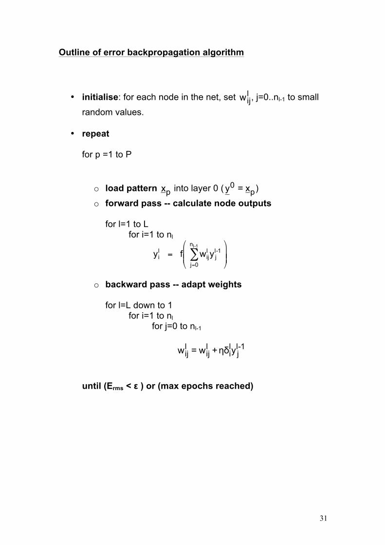
Outline of error backpropagation algorithm

• initialise: for each node in the net, set lijw , j=0..nl-1 to small

random values. • repeat

for p =1 to P

o load pattern px into layer 0 ( p0 x=y )

o forward pass -- calculate node outputs

for l=1 to L for i=1 to nl

!

yil = f wij

l y jl-1

j=0

nl-1

" #

$ % %

&

' ( (

o backward pass -- adapt weights

for l=L down to 1 for i=1 to nl for j=0 to nl-1

1-lj

li

lij

lij yηδ+w=w

until (Erms < ε ) or (max epochs reached)

32

Notes

• Setting initial weights to small random values is important for MLP learning: large and/or very similar starting values impede learning. The MLP, although it is more powerful than the single layer perceptron, does not come with a guarantee of success; although it’s theoretically possible that a given net can learn to perform a particular function, in practice this may be prevented by a number of factors such as starting weight values or an over-large training rate (which causes the net not to even approximately follow the desired gradient descent path, theoretically only followed when η is infinitesimally small).

• How many layers and/or units do you use? It’s not

normally necessary to use more than one hidden layer, because there is a universal approximation theorem that says that any reasonable function can be learned by a two-layer net. But note the phase 'a two-layer net' -- this does not tell the user how many hidden neurons are needed for a given problem! Despite a lot of theoretical work, trial and error (with some consideration given to the 'overtraining' problem to be discussed later) is actually still the best way to determine this.

• Use of 'target error' ε: With MLP learning, unlike the case

of the single layer perceptron, it is not reasonable to expect the error to drop to exactly zero, partly because the use of the sigmoid function prevents output neurons (for any finite weight values) ever exactly reaching binary targets 0,1, and partly because problems to which the MLP is applied are usually intrinsically difficult. Also, it may not be desirable in any case to continue training until the training data error is as low as possible -- overtraining may well be a problem, and early stopping of the training process therefore advisable.

• Use of 'max epochs': If a problem’s level of difficulty is not

at first appreciated, it is easy to give the net a too-simple architecture (not enough hidden units) so that the anticipated target error cannot ever be reached; the 'max epochs' limit stops the training carrying on for an unreasonable length of time in this case.

33

PROBLEMS THAT CAN OCCUR WHEN TRAINING A MULTILAYER PERCEPTRON 1. Trapping in local minima Sometimes when training an MLP the final error reached is considerably higher than one might have expected. This can either be because the difficulty of the problem had been underestimated, or possibly be because the net had become trapped in a less-than-optimal solution known as a local minimum of the error function. The error-weight surface is usually very high-dimensional, potentially very complex, and can contain 'traps' for a net whose learning is based on gradient descent. The basic principle of gradient descent is to continue to go downhill until the surface seems flat -- but although this would be true at the lowest overall error position, the global minimum, it might also be true at some higher error positions, as illustrated schematically below: Where the net ends up is unavoidably a function of what part of the error-weight surface it starts off in; the set of initial positions leading to a particular final set of weights is referred to as the basin of attraction of that final position. There is no known way of ensuring that the net starts in the basin of attraction of the global minimum, it really is all down to chance! If a local minimum is suspected the best policy is to re-start the net with a different set of weights -- if it was a local minimum the first time, chances are that the net will do better, but if the problem is simply unexpectedly hard, the final error this second time will be very similar to the first.

34

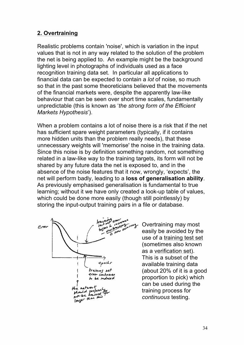
2. Overtraining Realistic problems contain 'noise', which is variation in the input values that is not in any way related to the solution of the problem the net is being applied to. An example might be the background lighting level in photographs of individuals used as a face recognition training data set. In particular all applications to financial data can be expected to contain a lot of noise, so much so that in the past some theoreticians believed that the movements of the financial markets were, despite the apparently law-like behaviour that can be seen over short time scales, fundamentally unpredictable (this is known as ‘the strong form of the Efficient Markets Hypothesis’). When a problem contains a lot of noise there is a risk that if the net has sufficient spare weight parameters (typically, if it contains more hidden units than the problem really needs), that these unnecessary weights will 'memorise' the noise in the training data. Since this noise is by definition something random, not something related in a law-like way to the training targets, its form will not be shared by any future data the net is exposed to, and in the absence of the noise features that it now, wrongly, ‘expects’, the net will perform badly, leading to a loss of generalisation ability. As previously emphasised generalisation is fundamental to true learning; without it we have only created a look-up table of values, which could be done more easily (though still pointlessly) by storing the input-output training pairs in a file or database.

Overtraining may most easily be avoided by the use of a training test set (sometimes also known as a verification set). This is a subset of the available training data (about 20% of it is a good proportion to pick) which can be used during the training process for continuous testing.

35

At the end of each epoch of training the net is shown the training test set data and a forward pass only done on this, to evaluate, for that epoch, the rms error for this data set as well as for the training set. The shapes of the error curves for both the training and training test set data are monitored; when that for the training test set begins to rise (even though the error for the training set itself may still be decreasing) it is time to stop training as it is likely now that the net is improving on the training set by memorising the noise features it contains. One thing to note is that a strict approach to neural network training -- not always followed -- would also demand a third set of data, a true test set, to be used only when the net has been trained to completion (with possible ‘early stopping’ when the training test set error starts to rise). The argument is that the training test set, although it wasn’t used in an obvious way to guide the weight changes, was used in a subtle way because it determined when the training process should end. A true test set should ideally not be used in any way whatsoever to affect the training process. Which is more important in practice, trapping in local minima or overtraining? In most applications -- as mentioned above, especially in the noise-riddled area of finance -- I would say almost always overtraining. (In one example a financial problem allowed training only for 2 or 3 epochs before overtraining set in -- clearly in a case like this there is little chance of reaching any error minimum, either global or local!)

36

Assessing the results This section will look only at classifier nets, ones for which the target is a binary string that codes for which 'type' of input is present, since the majority of applications of neural networks are currently of this kind. Measuring the performance of a classifier net Reduction of the mean squared error is used to drive the weight change process primarily because of its mathematical properties: it is a differentiable (smooth) function that would be zero only if all network outputs were perfectly correct. However in reality training of an MLP will always end up with some residual error. Suppose you were comparing the results of training two different nets -- with, say, different numbers of hidden units -- one of which had a residual mean squared error twice as large as the other. By how much is the latter really to be preferred to the former? Is the mean squared error (or root mean squared error) actually the most useful performance measure in practice? For a classifier, probably not. The simplest classifier would just have one output neuron and be required to learn to output '1' for positive examples, '0' for negative examples. As an instance of such classifier training, consider the problem of predicting the circumstances under which a person with a speech difficulty will stutter. (This is something I have worked on in collaboration with Prof Peter Howell of the speech research group in UCL Psychology department, and final year CS project students, for a number of years.) The neural network’s task is to predict, from a numerical descriptor of word difficulty devised by Prof Howell, whether a person with a tendency to stutter will stutter when faced with a particular word. The positive examples here are cases where (from observation) the person did stutter, the negative examples where they did not. After training the net (possibly with early stopping to avoid overtraining) the net can be assessed on its test set by looking at the outputs it produced for each of these examples and scoring it as 'correct' if either

37

• the desired output was '0' and the net’s output was < 0.5 (correctly classified negative case)

• the desired output was '1' and the net’s output was ≥ 0.5 (correctly classified positive case)

The '0.5' here is the classification threshold, normally equidistant between the two targets. The most basic measure of success is to add up the number of correct classifications (in the above sense) and divide by the number of examples. Multiplying by 100 gives the percentage correct:

100examples of number

tionsclassifica correct of numberrate success ×=

Suppose the success rate of a net designed to predict when a person might stutter was 90%. A great result? Not necessarily... If 50% of the examples had been positive examples (where the person did stutter) this would definitely have been a very good result. But in practice even a person with a severe speech difficulty stutters only about 10% of the time, and in most of the data sets we had just 5-10% were positive examples -- the data sets were numerically unbalanced. In such cases some caution is called for. There is a particular kind of local minimum that nets with unbalanced data sets can fall into, that of assigning all examples to the majority set -- in this case, always outputting values below 0.5, implying that no-one would ever stutter on an example word. Assuming that people stuttered 10% of the time this would automatically give a net which was ‘90% correct’ although the net would be doing nothing useful at all.

38

CASE STUDY: using a neural net to predict bankruptcy (From the study of Dorsey et al., University of Missouri Business School, 1995, as cited in Siegel and Shim, 2003.) A neural network was used to predict which companies would become bankrupt during the year 1995, based on publicly available information (from America Online’s Financial Reports database) from the preceeding year 1994. Information about 20 companies was used to train the net, 10 of which did become bankrupt during 1995, 10 of which did not but were considered to be high-risk companies which had been showing some signs of financial distress. The input data took the form of various ratios between financial quantities which might have a bearing on the financial health of the companies. These financial ratios were chosen because they had been used since the 1960s to predict company insolvency (although within the context of statistical analyses, not neural network models). The 19 ratios used were as listed below: Cash flow/Total assets Cash flow/Total sales Cash flow/Total debt Current assets/Current liabilities Current assets/Total assets Current assets/Total sales Earnings before tax and interest/Total assets Retained earnings/Total assets Net income/Total assets Total debt/Total assets Total sales/Total assets Working capital/Total sales Working capital/Total assets Quick assets/Total assets Quick assets/Current liabilities Quick assets/Total sales Equity market value/Total capitalisation Income/Total assets Income/(Interest+15) Cash flow/Current liabilities

39

A target of '1' was used to denote that a company became bankrupt, a '0' that it didn’t (obviously training took place after the end of 1995 and was thus based on historical data about the fortunes of the 20 companies considered).

• Use of financial ratios

o These are quantities that had previously been shown useful in other prediction models -- GOOD.

o There are only 15 quantities making up the 19 ratios

used

Cash flow; Total assets; Total sales; Total debt; Current assets; Current liabilities; Earnings before tax and interest; Retained earnings; Net income; Working capital; Quick assets; Equity market value; Total capitalisation; Income; Interest+15

and moreover not all of these 15 are independent variables -- for example working_capital = (current_assets-current_liabilities). Mathematically one might therefore query this use of 19 ratios; some would seem unnecessary as they could be constructed from a knowledge of the others. However having information theoretically available to a neural net is not -- because of the likely complexity of its error-weight surface -- the same as being sure it will be able to make use of it. So especially as these quantities had in the past been found useful, the number of parameters is OKAY.

• Selection of companies on which to train the net

o Neural networks find it harder to deal with

positive/negative training sets of unbalanced sizes, so the choice to use just 10 examples of non-bankrupt companies (when there must have been very many more) is OKAY although there are more sophisticated ways to deal with this kind of situation.

o The choice to use 'financially distressed' negative

examples is GOOD -- the problem might have been made artificially easy otherwise.

40

Here are the results obtained by Dorsey et al.:

Company Bankrupt? (0=no, 1=yes)

Network output after training

Net correct? (threshold 0.4)

Apparel Ventures Inc. 0 0.3808 Yes Apple Computer Inc. 0 0.0027 Yes Biscayne Apparel Inc. 0 0.4315 NO Epitope Inc. 0 0.1824 Yes Montgomery Ward Holding Inc.

0 0.0627 Yes

Schwerman Trucking Co. 0 0.5782 NO Signal Apparel Co. 0 0.3708 Yes Southern Pacific Transportation

0 -0.3515 Yes

Time Warner Inc. 0 0.5783 NO Warner Insurance Services 0 -0.1020 Yes Baldwin Builders 1 0.5783 Yes Bradlees Inc. 1 1.0083 Yes Burlington Motor Holdings 1 1.0083 Yes Clothestime Inc. 1 0.4315 Yes Dow Corning 1 0.6552 Yes Edison Brothers Stores 1 0.6112 Yes Freymiller Trucking Co. 1 1.0083 Yes Lamonts Apparel Inc. 1 1.2896 Yes Plaid Clothing Group Inc. 1 1.2896 Yes Smith Corona Co. 1 0.4315 Yes

• Why are some of the net’s output values below 0.0, or above 1.0?

This is not a problem. Though most people use the sigmoid squashing function for all neurons in a network, including those in the output layer, the Universal Approximation Theorem (which sets out what multilayer perceptrons can do) only requires these functions to be used in the hidden layer(s) of the net; the output layer can be chosen to have 'linear' neurons (f(a)=a) whose output values can be any number. This was likely what was done in this case.

41

• Why are some of the net’s outputs the same for different companies? (eg Bradlees Inc., Burlington Motor Holdings, Freymiller Trucking Co. all have the output 1.2896 -- in fact in the numbers agreed to 8 significant figures...) This is odd. The only way this would be likely to happen is if these companies were described by exactly the same 19 ratios. That seems to me improbable. Without seeing the original data I can’t say that this is actually wrong, but if I had trained the net and got this result I would be taking a very careful look at my data files.

• Where’s the test set?

The results presented appear to be for the training set -- this, as the discussion of 'overtraining' made clear, is not necessarily a guide as to how the net would perform on new data (ie some further companies for which ratio data for 1994 was available, and whose financial fate during 1995 was known). Presenting only training set results is very bad practice, especially in a case like this where there is a high likelihood of overtraining occurring because the number of training patterns (only 20) is small compared with the size of the network. (Ideally one should have at least 10x as many training patterns as weights in the net, which here would imply a demand for 100s-1000s of examples.)

• Are the results as good as were claimed?

The authors made a point of noting that their net was '100% correct for those companies that went bankrupt.' However following the discussion related to unbalanced training sets (although here there were equal numbers of representatives of both classes) you will realise that this would also be true if the net had predicted that every company would become bankrupt in 1995!

42

References for this section: • Russell Beale and Tom Jackson, Neural Computing: An introduction, Institute of Physics Press, 1990. • Joel Siegel and Jae Shim, The Artificial Intelligence Handbook: Business applications in accounting, banking, finance, management and marketing, Thomson, 2003. • http://www.aaai.org American Association for Artificial Intelligence (AAAI).