1

Introduction to MVC

Definition---Properness and strictly properness

A system G(s) is proper if all its elements { ( )}ijg s are proper, and strictly proper

if all its elements are strictly proper.

Definition---Causal

A system G(s) is causal if all its elements are causal, and not causal if all its

elements are noncausal.

Definition---Poles

The eigen values iλ , i=1,---,n of the system G(s) are called the pole of the system.

The pole polynomial ( )sπ is defined as:1

( ) ( )n

ii

s sπ λ=

= −∏ , where ( )sπ is the

least common denominator of all non-identical-zero minors of all order of G(s).

Example:

2( 1)( 2) 0 ( 1)1

( )( 1)( 2)( 1)

( 1)( 2) ( 1)( 1) ( 1)( 1)

s s s

G ss s s

s s s s s s

− + − = + + − − + + − + − +

The minor of order 2:

1,2 1,2 1,21,2 1,3 2,3 2

1 2 ( 1); ;

( 1)( 2) ( 1)( 2) ( 1)( 2)

sG G G

s s s s s s

− −= = =+ + + + + +

The least common denominator of the minors:

2( ) ( 1)( 2) ( 1)s s s sπ = + + −

Definition---Zeros

If the rank of G(z) is less than the normal rank, z is a zero of the system. The

zero polynomial Z(s) is the greatest common divisor of the numerators of all

order-r minors of G(s), where r is the norminal rank of G(s) provided that these

minors have all been adjusted in such a way as to have the pole polynomial

( )sπ as their denominator.

2

1,2 1,2 1,21,2 1,3 2,3

( 1)( 2) 2( 1)( 2) ( 1)( ) ; ( ) ; ( )

( ) ( ) ( )

s s s s sG s G s G s

s s sπ π π− + − + − −= = =

So, ( ) ( 1)Z s s= −

According to this definition, the zero polynomial of a square G(s) is:

det{ ( )} 0G s =

Notice that, in a MIMO system, there may be no inverse response to indicate the

2

presence of RHP-zero. For example, in the MIMO system of the following:

{ }1 11( ) ; (0.5) 0; (0.5) 0

1 2 2(0.2 1)( 1)

0.45 0.89 1.92 0 0.71 0.711(0.5)

0.89 0.45 0 0 0.71 0.711.65H

H

U V

G s G Gss s

G

σ

Σ

= = = ++ +

− = − 1442443142431442443

Transfer functions for Closed loop MIMO systems

1. Cascade rule. For the cascade interconnection of 1( )G s and 2 ( )G s in the

following figure(a), the overall transfer function matrix is G=G1G2

2. Feedback rule. With reference to the positive feedback system in Figure (b):

1 12 1( ) ( )v I L u I G G u− −= − = −

3. Push-through rule. 1 11 2 1 1 2 1( ) ( )G I G G I G G G− −− = −

1 1 2 1 1 2 1 1 2 1

11 2 1 2 1 1

1 11 2 1 1 2 1

( ) ( )

( ) ( )

( ) ( )

G G G G G I G G I G G G

I G G G I G G G

I G G G G I G G

−

− −

− = − = −

⇒ − − =

⇒ − = −

3

4. MIMO rule.

(1). Start from the output, write down the blocks as moving backward by the most

direct path toward the input

(2). When exit from a feedback loop, include a term (I-L)-1 for positive feedback

(or, (I+L)-1 for negative feedback. Notice that L is the evaluated against signal

flow starting at the point of exit from the loop.

Example: Consider the following block diagram:

111 12 22 21(1 )z p p K P K p w− = + −

5. Consider the closed-loop system:

The following relationships are useful:

1 1

1 1

1 1 1

1 1 1 1

( ) ( ) 1

( ) ( )

( ) ( ) ( )

( ) ( ) ( )

I L L I L S T

G I KG I GK G

GK I GK G I KG K I GK GK

T L I L I L L I L

− −

− −

− − −

− − − −

+ + + = + =+ = +

+ = + = += + = + = +

4

Singular Values and Matrix Norms

1. Vector Norms

A real valued function • defined on a vector space X is said to be a norm on

X, if it satisfies the following properties:

(1) 0x ≥ ;

(2) 0x = only if 0x = ;

(3) , for any scalar ;x xα α α=

(4) x y x y+ ≤ + ;

for any and .x X y X∈ ∈

The vector p-norm of x X∈ is defined as: 1/

1

, for 1 .n

p

ipi

x x p=

= ≤ ≤ ∞ ∑ In

particular 1, 2, we have:p = ∞

11

n

ii

x x=

=∑ ; ( )2

21

| |n

ii

x x=

= ∑ ; 1max i

i nx x

∞ ≤ ≤= .

H o&& lder inequality:

1 1, 1T

p qx y x y

p q≤ + =

Notice that:

(1) 2 1 2

x x n x≤ ≤ ;

(2) 2

x x n x∞ ∞

≤ ≤ ;

(3) 1

x x n x∞ ∞

≤ ≤

5

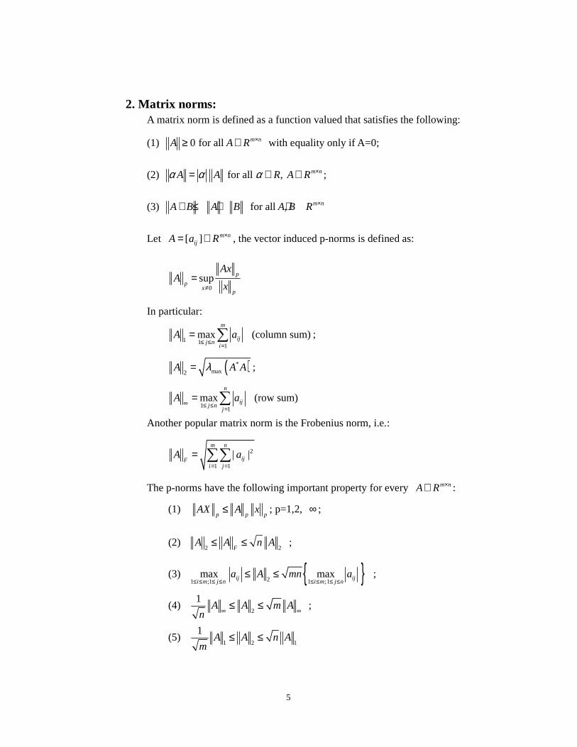
2. Matrix norms: A matrix norm is defined as a function valued that satisfies the following:

(1) 0 for all m nA A R ×≥ ∈ with equality only if A=0;

(2) for all , m nA A R A Rα α α ×= ∈ ∈ ;

(3) for all , m nA B A B A B R ×+ ≤ + ∈

Let [ ] m nijA a R ×= ∈ , the vector induced p-norms is defined as:

0

sup p

px

p

AxA

x≠=

In particular:

1 1

1

max (column sum)m

ijj n

i

A a≤ ≤ =

= ∑ ;

( )*max2

A A Aλ= ;

1

1

max (row sum)n

ijj n

j

A a∞ ≤ ≤ =

= ∑

Another popular matrix norm is the Frobenius norm, i.e.:

2

1 1

| |m n

ijFi j

A a= =

= ∑∑

The p-norms have the following important property for every m nA R ×∈ :

(1) p p p

AX A x≤ ; p=1,2, ∞ ;

(2) 2 2F

A A n A≤ ≤ ;

(3) { }21 ;1 1 ;1max maxij ij

i m j n i m j na A mn a

≤ ≤ ≤ ≤ ≤ ≤ ≤ ≤≤ ≤ ;

(4) 2

1A A m A

n ∞ ∞≤ ≤ ;

(5) 1 2 1

1A A n A

m≤ ≤

6

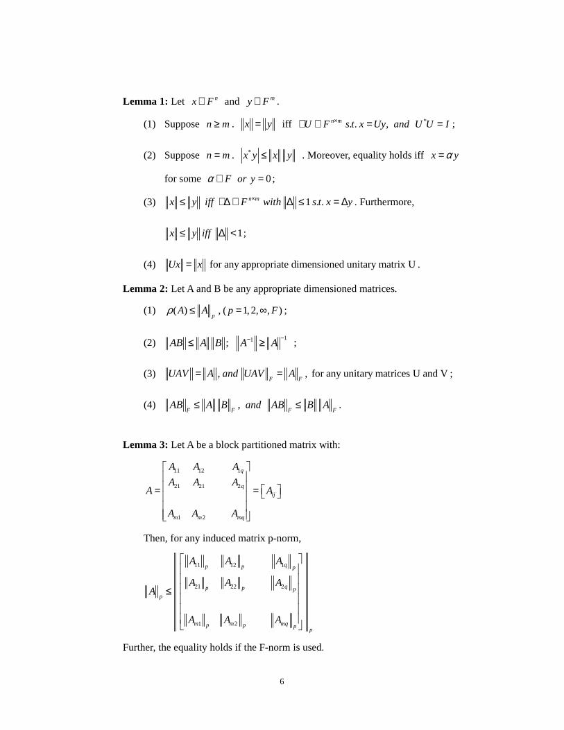
Lemma 1: Let nx F∈ and my F∈ .

(1) Suppose n m≥ . x y= iff *. . ,n mU F s t x Uy and U U I×∃ ∈ = = ;

(2) Suppose n m= . *x y x y≤ . Moreover, equality holds iff x yα=

for some 0F or yα ∈ = ;

(3) 1 . .n mx y iff F with s t x y×≤ ∃∆ ∈ ∆ ≤ = ∆ . Furthermore,

1x y iff≤ ∆ < ;

(4) for any appropriate dimensioned unitary matrix UUx x= .

Lemma 2: Let A and B be any appropriate dimensioned matrices.

(1) ( ) , ( 1, 2, , )p

A A p Fρ ≤ = ∞ ;

(2) 11;AB A B A A

−−≤ ≥ ;

(3) , , for any unitary matrices U and VF F

UAV A and UAV A= = ;

(4) ,F F F F

AB A B and AB B A≤ ≤ .

Lemma 3: Let A be a block partitioned matrix with:

11 12 1

21 21 2

1 2

q

q

ij

m m mq

A A A

A A AA A

A A A

= =

Then, for any induced matrix p-norm,

11 12 1

21 22 2

1 2

qp p p

qp p pp

m m mqp p pp

A A A

A A AA

A A A

≤

Further, the equality holds if the F-norm is used.

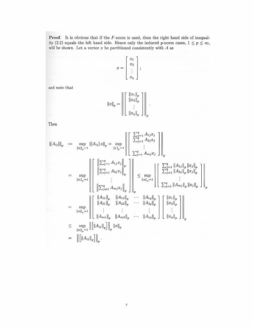
7

8

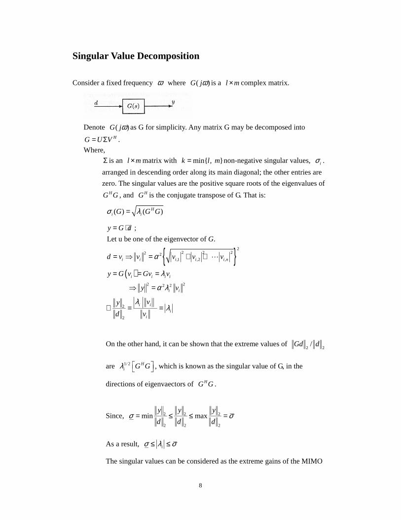
Singular Value Decomposition

Consider a fixed frequency ω where ( )G jω is a l m× complex matrix.

Denote ( )G jω as G for simplicity. Any matrix G may be decomposed into HG U V= Σ .

Where,

Σ is an l m× matrix with min{ , }k l m= non-negative singular values, iσ .

arranged in descending order along its main diagonal; the other entries are

zero. The singular values are the positive square roots of the eigenvalues of HG G , and HG is the conjugate transpose of G. That is:

( ) ( )Hi iG G Gσ λ=

{ }( )

22 2 22 2

,1 ,2 ,

2 22 2

2

2

;

Let u be one of the eigenvector of .

i i i i i n

i i i i

i i

i i

ii

y G d

G

d v v v v v

y G v Gv v

y v

vy

d v

α

λ

α λ

λλ

= ⋅

= ⇒ = + +

= = =

⇒ =

∴ = =

L

On the other hand, it can be shown that the extreme values of 2 2

/Gd d

are 1/ 2 Hi G Gλ , which is known as the singular value of G, in the

directions of eigenvaectors of HG G .

Since, 2 2 2

2 2 2

min maxy y y

d d dσ σ= ≤ ≤ =

As a result, iσ λ σ≤ ≤

The singular values can be considered as the extreme gains of the MIMO

9

system, which are local maximal values with respect to the direction of

inputs. For example, consider the gain matrix at a specific frequency:

5 4

3 2G

=

The gains with respect to the direction of d are given in the following

figure:

Typical singular values with respect to frequency are as shown in the

following figure:

Theorem 1: Let m nA F ×∈ . There exist unitary matrices:

1 2 1 2[ , , , ] ; [ , , , ]m m n nm nU u u u F V v v v F× ×= ∈ = ∈L L

such that: 1* 0,

0 0A U V

Σ = Σ Σ =

where,

{ }1

21 1 2

0 0

0 0; 0 ; min ,

0 0

p

p

p m n

σσ

σ σ σ

σ

Σ = ≥ ≥ ≥ ≥ =

L

LL

M M O M

L

10

[Proof]

Let Aσ = , and assume m n≥ .

Then, from the definition of A , i.e.:

( )sup ; 1,2, for some p

p p p pp

AzA p Az A z z

z= = ∞ ⇒ =

In other words, there exists a vector nz F∈ such that

Az z zσ σ= =

By the Lemma

( * iff there is a matrix such that and m nx y U F x Uy U U I×= ∈ = = )

there is a matrix m nU F ×∈% such that *U U I=% % and

( )Az U z Uzσ σ= =% % .

Let: nzx F

z= ∈ and mUz

y FUz

= ∈%

%

We have: 2 2Az Uz Uz Uz Uz

Ax yz AzAz Uz Uz

σ σ σσ

σ

= = = = = =

% % % %

% %

Let 1 1[ , ] ; [ , ]m m n nU y U F V x V F× ×= ∈ = ∈ be unitary.

Thus,

* *1 1 1

* * * *1 1

* * * *1 1 1 1 1 1

*

[ , ] [ , ]

0

A U AV y U Ax AV

y Ax y AV y y y AV

U Ax U AV U y U AV

w

B

σσ

σ

= =

= =

=

Since,

2

22 * 2 *1 1

2

1

0

0

A w w A w wσ σ

= + ⇒ ≥ +

M

11

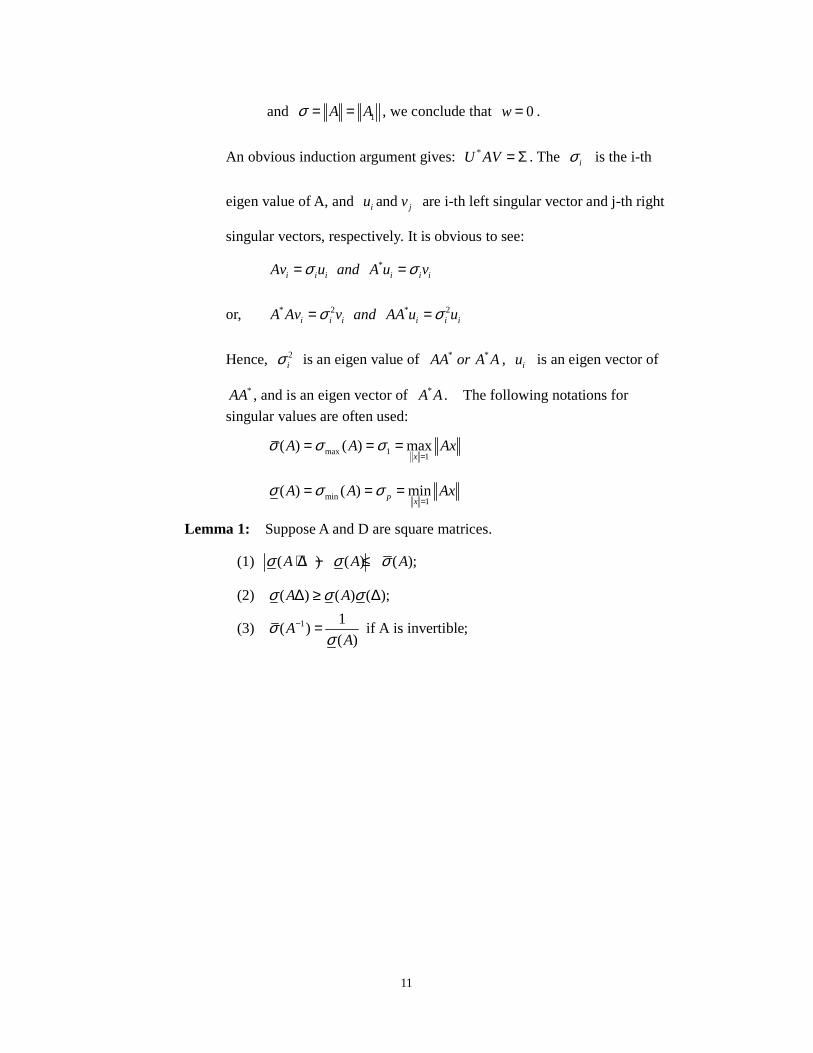
and 1A Aσ = = , we conclude that 0w = .

An obvious induction argument gives: *U AV = Σ . The iσ is the i-th

eigen value of A, and andi ju v are i-th left singular vector and j-th right

singular vectors, respectively. It is obvious to see:

*i i i i i iAv u and A u vσ σ= =

or, * 2 * 2i i i i i iA Av v and AA u uσ σ= =

Hence, 2iσ is an eigen value of * *AA or A A , iu is an eigen vector of

*AA , and is an eigen vector of *A A . The following notations for

singular values are often used:

max 11

( ) ( ) maxx

A A Axσ σ σ=

= = =

min1

( ) ( ) minpx

A A Axσ σ σ=

= = =

Lemma 1: Suppose A and D are square matrices.

(1) ( ) ( ) ( );A A Aσ σ σ+ ∆ − ≤

(2) ( ) ( ) ( );A Aσ σ σ∆ ≥ ∆

(3) 1 1( ) if A is invertible;

( )A

Aσ

σ− =

12

13

Lemma 3:

(1) ( ) ( )A Aσ λ σ≤ ≤

(2) p

Aλ ≤

(3) Let ( )

( ) condition number of ( )

AA A

A

σκσ

= = , and Ax b= . If

14

( ) ( )A x x b bδ δ+ = + , then: ( )x b

Ax b

δ δκ

= ×

(4) Let and A A A x x xδ δ→ + = +% % , where A and x satify Ax b= . Then:

( )

1 ( )

x A

x AA

A

δ κδ

κ≤

−

Thus, when ( )Aκ is large and matrix A is almost singular, a very

small change of A will make the possible range of xδ large.

15

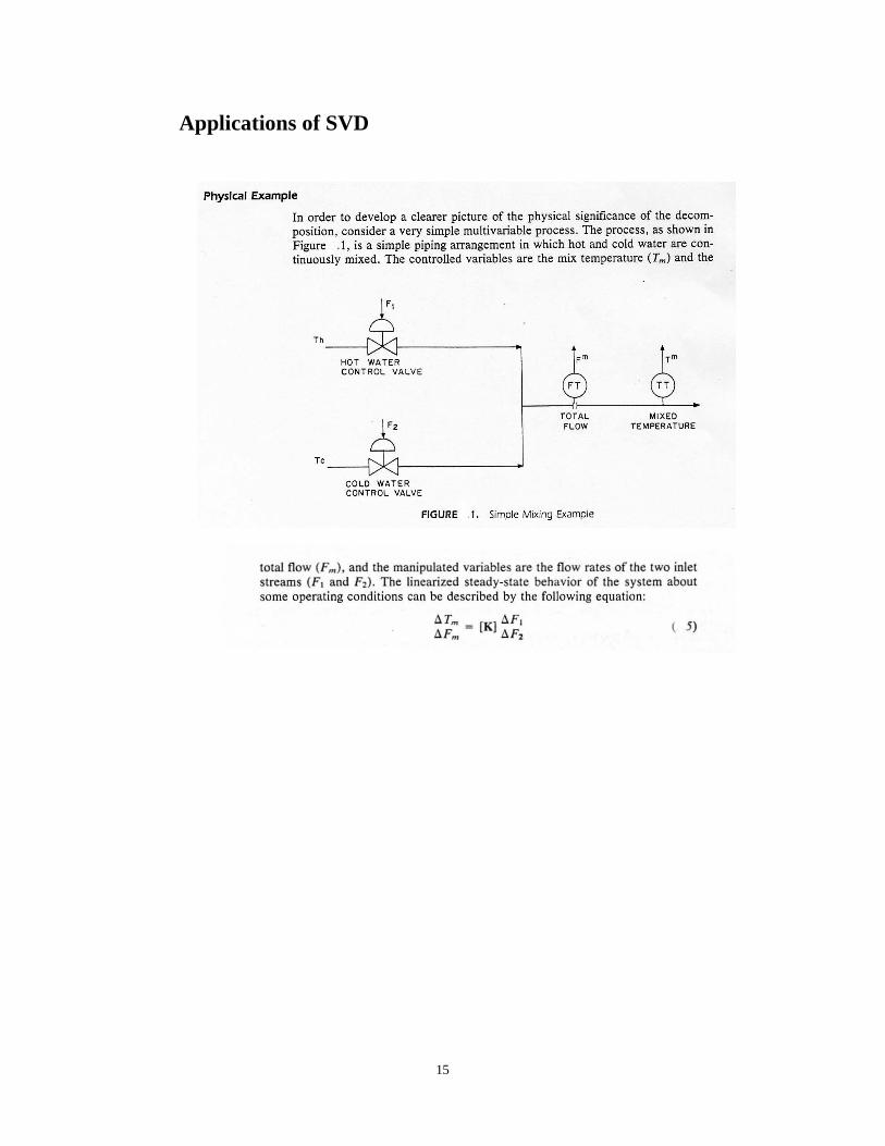
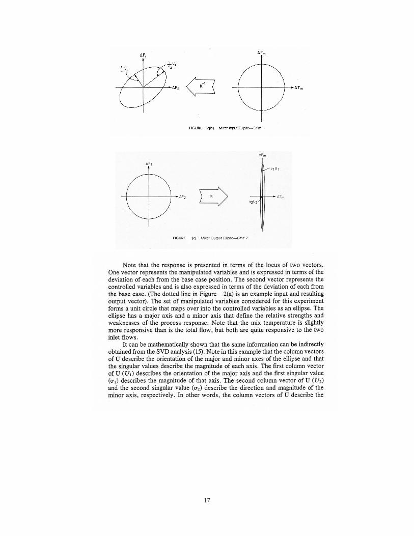
Applications of SVD

16

17

18

19

Problem of small singular values:

Very small singular values in a multivariable system are analogus to very

small gains in a conventional siso system. It requires very large

controller gains and results in excessively large controller actions. The

typical presence of constraints in the manipulated variable and noise in

the sensor makes it difficult even for siso system. In the context of mimo

system, the additional complications presented by hidden loops,

interactions make the problem even more severe.

A general rule of thumb to measure the small singular value is the

magnitude of the noise in the signal. Singular values are equal or less

than the magnitude of sensor noise should be assumed degenerate.

Problem of large singular values:

Large singular values are not as serious a problem as small values. It

requires very small controller gains. This results in small controller

outputs, which can be easily become lost in the resolution of the

manipulator. The symptomatic behaviors are cyclic responses, which

never settling down to a reasonable steady state.

A general rule of thumb concerning large singular values is that all

singular values that are equal to or greater than the reciprocal of the

valve resolution should be avoided.

Determining Good Sensor Locations

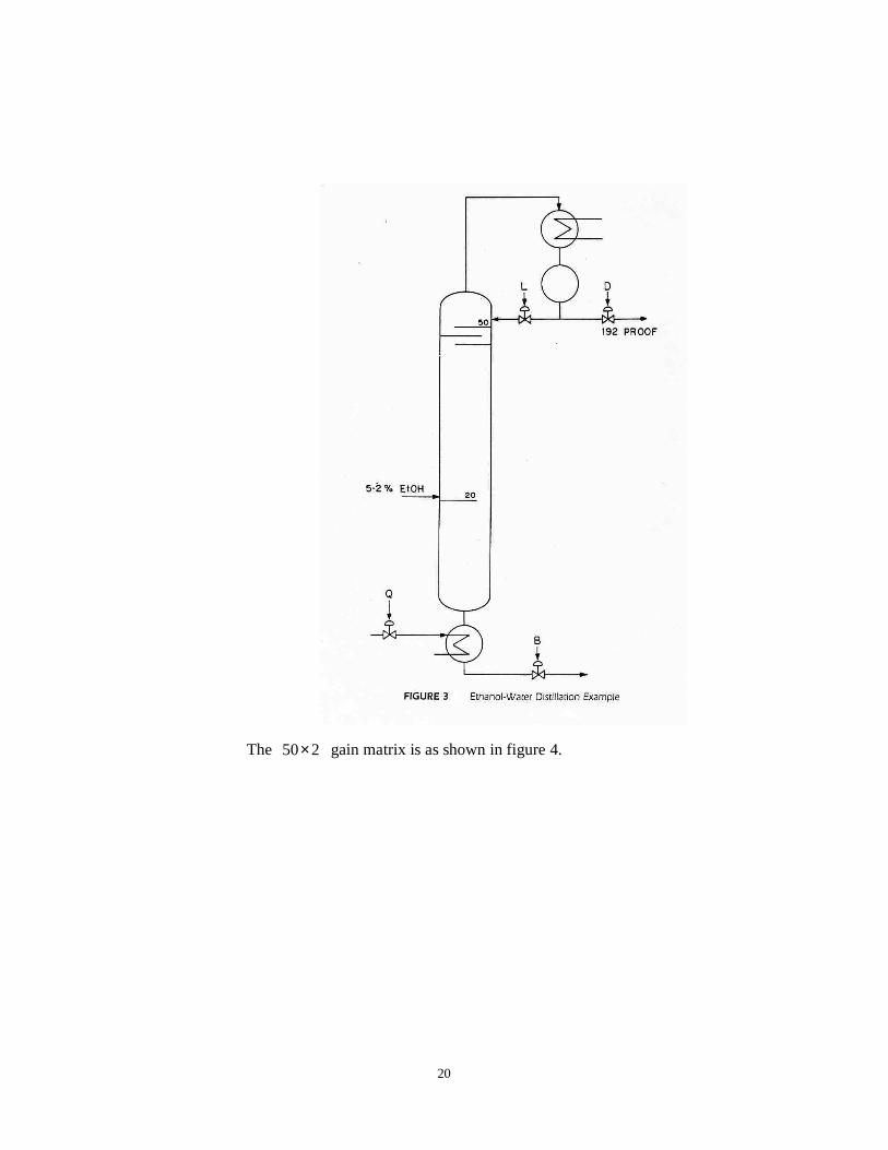
Consider, for example, the ethonal-water distillation column as shown in

Figure 3.Assume that the first level objective is to control two column

temperatures by manipulating D and Q. The basic concern is to

determine which combination out of 1225 possible combinations of

sensor locations from the point of view of column control.

20

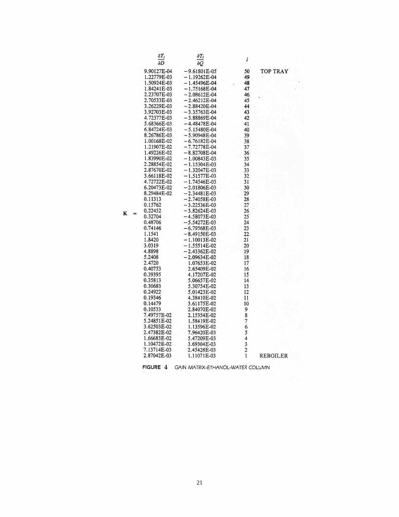
The 50 2× gain matrix is as shown in figure 4.

21

22

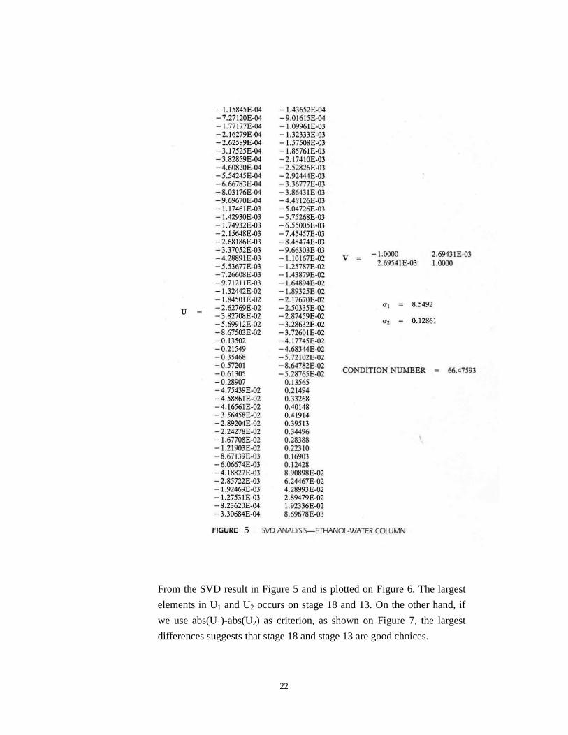
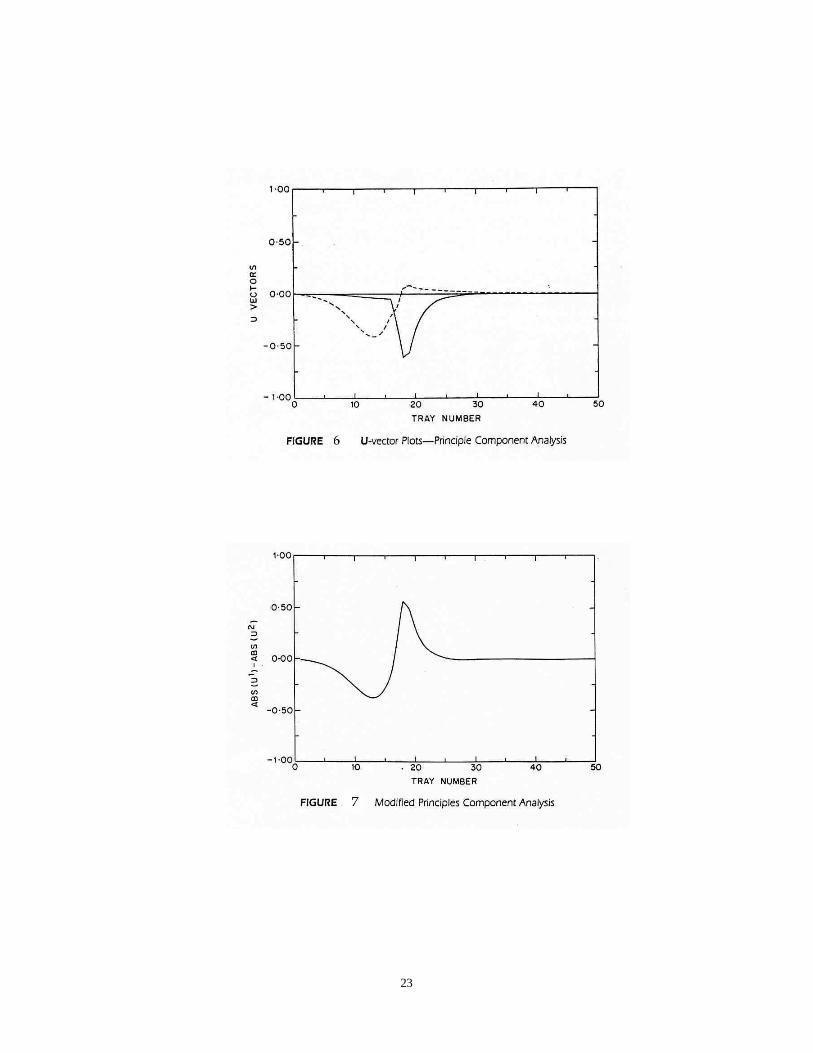
From the SVD result in Figure 5 and is plotted on Figure 6. The largest

elements in U1 and U2 occurs on stage 18 and 13. On the other hand, if

we use abs(U1)-abs(U2) as criterion, as shown on Figure 7, the largest

differences suggests that stage 18 and stage 13 are good choices.

23

24

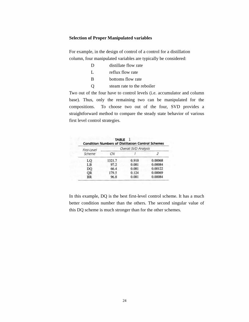
Selection of Proper Manipulated variables

For example, in the design of control of a control for a distillation

column, four manipulated variables are typically be considered:

D distillate flow rate

L reflux flow rate

B bottoms flow rate

Q steam rate to the reboiler

Two out of the four have to control levels (i.e. accumulator and column

base). Thus, only the remaining two can be manipulated for the

compositions. To choose two out of the four, SVD provides a

straightforward method to compare the steady state behavior of various

first level control strategies.

In this example, DQ is the best first-level control scheme. It has a much

better condition number than the others. The second singular value of

this DQ scheme is much stronger than for the other schemes.

25

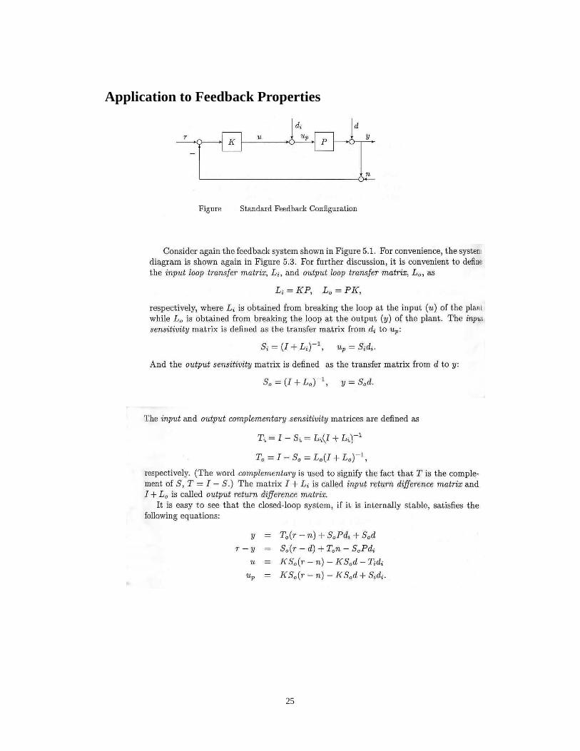
Application to Feedback Properties

26

27

Use of the minimum singular value of the plant: The minimum singular

value of the plant evaluated as a function of frequency is a useful measure for

evaluating the feasibility of achieving acceptable control. In general, we want

σ as large as possible.

Singular values for performance: In general, it is reasonable to require that

the gain 2 2

( ) / ( )e rω ω remains small for any direction of ( )r ω , including

the worst-case direction which gives a gin of ( ( ))S jσ ω . Let 1/ ( )pw jω

represent the maximum allowable magnitude of 2 2

( ) / ( )e rω ω at each

frequency, This results in the following performance requirement:

{ }1( ( )) , ( ) 1, ( 1

( )p p

p

S j w S j w S jw j

σ ω ω σ ω ω ωω ∞

< ∀ ⇔ < ∀ ⇔ <

Typical weight function is given asL

/

( ) bp

b

s Mw s

s A

ωω+=

+

which means 1/ pw equals 1A ≤ at low frequencies, and equals to 1M ≥

at high frequencies, and the asymptote crosses 1 at bω (the bandwidth

frequency).