Introduction to MATLAB®...Introduction To Matlab 2 Distribution A. TABLE OF CONTENTS Table of...
154
DISTRIBUTION A: Approved for public release; distribution unlimited. Approval given by 88 ABW/PA, 88ABW- 2018-4817, 02 Oct 2018. Developed by: Aaron J. Brumbaugh [email protected] Summer 2018 Introduction to MATLAB® Instructional Unit
Transcript of Introduction to MATLAB®...Introduction To Matlab 2 Distribution A. TABLE OF CONTENTS Table of...

DISTRIBUTION A: Approved for public release; distribution unlimited. Approval given by 88 ABW/PA, 88ABW- 2018-4817, 02 Oct 2018.
Developed by:
Aaron J. Brumbaugh
Summer 2018
Introduction to MATLAB®
Instructional Unit

Introduction To Matlab 2 Distribution A.
TABLE OF CONTENTS
Table of Contents................................................................................................................................................... 2
1. Mathematics and Variables in Matlab ® (Part 1) ............................................................................................ 6
1.1. Introduction ................................................................................................................................................. 6
1.2. Materials ...................................................................................................................................................... 6
1.3. Overview of Plan .......................................................................................................................................... 6
1.3.1. Learning Target – MATLAB.1 ............................................................................................................... 6
1.3.2. Learning Target – MATLAB.2 ............................................................................................................... 7
1.3.3. Learning Target – MATLAB.3 ............................................................................................................... 7
1.3.4. Learning Target – MATLAB.4 ............................................................................................................... 8
1.4. Guided Notes ............................................................................................................................................... 8
1.5. Assessment – Practice Problems ................................................................................................................ 12
1.6. Answer Keys ............................................................................................................................................... 14
1.6.1. Guided Notes ..................................................................................................................................... 14
1.6.2. Practice Problems .............................................................................................................................. 17
1.7. Resources ................................................................................................................................................... 21
Mathematics and Variables in Matlab ® (Part 2) .................................................................................................. 22
1.8. Introduction ............................................................................................................................................... 22
1.9. Materials .................................................................................................................................................... 22
1.10. Overview of Plan ........................................................................................................................................ 22
1.10.1. Learning Target – MATLAB.5 ............................................................................................................. 22
1.11. Guided Notes ............................................................................................................................................. 23
1.12. Assessment – Practice Problems ................................................................................................................ 26
1.13. Answer Keys ............................................................................................................................................... 28
1.13.1. Guided Notes ..................................................................................................................................... 28
1.13.2. Practice Problems .............................................................................................................................. 31
1.14. Resources ................................................................................................................................................... 32
Creating Scripts in MATLAB® ................................................................................................................................ 33
1.15. Introduction ............................................................................................................................................... 33
1.16. Materials .................................................................................................................................................... 33
1.17. Overview of Plan ........................................................................................................................................ 33
1.17.1. Learning Target – MATLAB.6 ............................................................................................................. 33
1.17.2. Learning Target – MATLAB.7 ............................................................................................................. 33
1.17.3. Learning Target – MATLAB.8 ............................................................................................................. 34
1.18. Guided Notes ............................................................................................................................................. 34
1.19. Assessment – Practice Problems ................................................................................................................ 37
1.20. Answer Keys ............................................................................................................................................... 39

Introduction To Matlab 3 Distribution A.
1.20.1. Guided Notes ..................................................................................................................................... 40
1.20.2. Practice Problems .............................................................................................................................. 43
1.21. Resources ................................................................................................................................................... 46
Comments and Formatting Strings ....................................................................................................................... 47
1.22. Introduction ............................................................................................................................................... 47
1.23. Materials .................................................................................................................................................... 47
1.24. Overview of Plan ........................................................................................................................................ 47
1.24.1. Learning TargeT – MATLAB.9 ............................................................................................................ 47
1.24.2. Learning Target – MATLAB.10 ........................................................................................................... 48
1.25. Guided Notes ............................................................................................................................................. 48
1.26. Assessment – Practice Problems ................................................................................................................ 53
1.27. Answer Keys ............................................................................................................................................... 55
1.27.1. Guided Notes ..................................................................................................................................... 55
1.27.2. Practice Problems .............................................................................................................................. 60
1.28. Resources ................................................................................................................................................... 63
Matrices and Matrix Operations .......................................................................................................................... 64
1.29. Introduction ............................................................................................................................................... 64
1.30. Materials .................................................................................................................................................... 64
1.31. Overview of Plan ........................................................................................................................................ 64
1.31.1. Learning Target – MATLAB.11 ........................................................................................................... 64
1.31.2. Learning Target – MATLAB.12 ........................................................................................................... 64
1.31.3. Learning Target – MATLAB.13 ........................................................................................................... 65
1.31.4. Learning Target – MATLAB.14 ........................................................................................................... 65
1.32. Guided Notes ............................................................................................................................................. 66
1.33. Assessment – Practice Problems ................................................................................................................ 70
1.34. Answer Keys ............................................................................................................................................... 71
1.34.1. Guided Notes ..................................................................................................................................... 72
1.34.2. Practice Problems .............................................................................................................................. 76
1.35. Resources ................................................................................................................................................... 78
Graphing in MATLAB® .......................................................................................................................................... 79
1.36. Introduction ............................................................................................................................................... 79
1.37. Materials .................................................................................................................................................... 79
1.38. Overview of Plan ........................................................................................................................................ 79
1.38.1. Learning Target – MATLAB.15 ........................................................................................................... 79
1.38.2. Learning Target – MATLAB.16 ........................................................................................................... 80
1.38.3. Learning Target – MATLAB.17 ........................................................................................................... 80
1.39. Guided Notes ............................................................................................................................................. 81
1.40. Assessment – Practice Problems ................................................................................................................ 85

Introduction To Matlab 4 Distribution A.
1.41. Answer Keys ............................................................................................................................................... 86
1.41.1. Guided Notes ..................................................................................................................................... 86
1.41.2. Practice Problems .............................................................................................................................. 91
1.42. Resources ................................................................................................................................................... 93
Conditional Statements in MATLAB® ................................................................................................................... 94
1.43. Introduction ............................................................................................................................................... 94
1.44. Materials .................................................................................................................................................... 94
1.45. Overview of Plan ........................................................................................................................................ 94
1.45.1. Learning Target – MATLAB.18 ........................................................................................................... 94
1.45.2. Learning Target – MATLAB.19 ........................................................................................................... 95
1.45.3. Learning Target – MATLAB.20 ........................................................................................................... 95
1.46. Guided Notes ............................................................................................................................................. 96
1.47. Assessment – Practice Problems .............................................................................................................. 103
1.48. Answer Keys ............................................................................................................................................. 105
1.48.1. Guided Notes ................................................................................................................................... 105
1.48.2. Practice Problems ............................................................................................................................ 113
1.49. Resources ................................................................................................................................................. 116
Introduction to Loops: For Loops ....................................................................................................................... 117
1.50. Introduction ............................................................................................................................................. 117
1.51. Materials .................................................................................................................................................. 117
1.52. Overview of Plan ...................................................................................................................................... 117
1.52.1. Learning Target – MATLAB.21 ......................................................................................................... 117
1.52.2. Learning Target – MATLAB.22 ......................................................................................................... 118
1.53. Guided Notes ........................................................................................................................................... 118
1.54. Assessment – Practice Problems .............................................................................................................. 124
1.55. Answer Keys ............................................................................................................................................. 126
1.55.1. Guided Notes ................................................................................................................................... 126
1.55.2. Practice Problems ............................................................................................................................ 133
1.56. Resources ................................................................................................................................................. 136
Introduction to Loops: While Loops ................................................................................................................... 137
1.57. Introduction ............................................................................................................................................. 137
1.58. Materials .................................................................................................................................................. 137
1.59. Overview of Plan ...................................................................................................................................... 137
1.59.1. Learning Target – MATLAB.23 ......................................................................................................... 137
1.59.2. Learning Target – MATLAB.24 ......................................................................................................... 138
1.60. Guided Notes ........................................................................................................................................... 138
1.61. Assessment – Practice Problems .............................................................................................................. 143
1.62. Answer Keys ............................................................................................................................................. 145

Introduction To Matlab 5 Distribution A.
1.62.1. Guided Notes ................................................................................................................................... 145
1.62.2. Practice Problems ............................................................................................................................ 151
1.63. Resources ................................................................................................................................................. 154
1.64. Image Credits ........................................................................................................................................... 154

Introduction To Matlab 6 Distribution A.
1. MATHEMATICS AND VARIABLES IN MATLAB ® (PART 1)
Primary Resource (if applicable): https://www.mathworks.com/help/matlab/
1.1. INTRODUCTION
Briefly describe the lesson/unit and/or provide background information and context.
The first lesson of Introduction to MATLAB® provides an overview of the MATLAB®
programming environment, performing mathematical calculations in the command window,
and working with variables.
1.2. MATERIALS
Each student will need:
PC/Mac with MATLAB® installed
Copy of Introduction to MATLAB® - Mathematics and Variables in MATLAB® (Part 1)
guided notes (these may be printed or shared digitally):
https://padlet.com/abrumbaugh/introMatlab
The teacher will need:
PC/MAC with MATLAB® installed
Ceiling projector or method for displaying their computer screen for students to see
Copy of Introduction to MATLAB® - Mathematics and Variables in MATLAB® (Part 1)
answer key
1.3. OVERVIEW OF PLAN
This lesson can be taught via direct instruction or student-paced learning through online videos
located at https://padlet.com/abrumbaugh/introMatlab.
1.3.1. LEARNING TARGET – MATLAB.1
Be able to describe MATLAB® and its general capabilities.
Students should understand that MATLAB® is a computational programming language that is
used in the fields of science, engineering, and many others for a variety of reasons. The
software allows users to perform a wide variety of calculations from simple to complex and has
a strong, yet natural, programming environment that allows users to automate their work.
MATLAB® is very beneficial as it can quickly calculate a series of computations on a large set of

Introduction To Matlab 7 Distribution A.
data, create easy-to-read dynamic models, and run complex simulations that help users better
understand the real world phenomena that they are studying.
1.3.2. LEARNING TARGET – MATLAB.2
Be able to identify the different parts of the MATLAB® window and explain what they do.
Students should have a general understanding of the MATLAB® window that is displayed on the
screen when they run the program. This is very important as some of the materials for this unit
will refer to specific parts of the window such as the editor or command window.
The current folder section displays any MATLAB® files that are in the working directory. The
working directory is initially set up to the MATLAB® folder when the software is installed on the
computer, however it can be changed at any time. Any files saved outside of the working
directory will not be found by MATLAB® and thus inaccessible. It is recommended that students
save or move their work to the working directory of MATLAB®.
The command window is a space where students can type individual commands to see what
they do. It is ideal for testing out a specific line of code to see what it does or single line
calculations. The command window is also where the output of any script/program created in
the editor will display.
The editor is where scripts (i.e., programs) are created. If a problem requires multiple
calculations or commands to be done in succession, the editor is the space to be working in. It is
also important to note that work in the editor can be saved as an .m file (MATLAB®’s file type)
and used again later, whereas work in the command window cannot be saved. The editor will
run any lines of code written in the space from the top down, one line at a time until it reaches
the end of the script.
The workspace is an area of the MATLAB® window that displays any variables that have been
created by the command window or editor. Along with the variable names, students will be
able to see the current value of each variable as well as the type of each variable (e.g., double,
logical).
1.3.3. LEARNING TARGET – MATLAB.3
Be able to perform basic mathematical operations in MATLAB®.
Throughout this course, students will use a variety of mathematical operations in MATLAB®
ranging from basic (e.g., addition, subtraction) to more advanced (e.g., modular arithmetic,
trigonometry). In this first lesson, students need to become familiar with performing addition,

Introduction To Matlab 8 Distribution A.
subtraction, multiplication, and division, as they are the backbone to many of the problems that
appear throughout this unit. Furthermore, students will need to understand and be able to
follow many of the calculations in this lesson and throughout the unit.
It is important to note that one issue that may arise with this learning target is with regards to
multiplication. MATLAB® does not execute “implied” multiplication such as 2(3). Typing such
an expression into the command window would result in a syntax error. Students will need to
explicitly type an asterisk (*) to tell MATLAB® to multiply the two numbers (e.g., 2 ∗ 3).
1.3.4. LEARNING TARGET – MATLAB.4
Be able to declare and use variables in MATLAB®.
Like most programming languages, MATLAB® uses variables in its programming features.
Students should understand that variables are used to store data that is either user defined or
generated within a program. The values stored in a variable can be recalled and used later in a
program.
It is important that students understand how to declare a variable, that is, how to assign a
specific value or expression to a variable. When declaring a variable, the variable’s name should
come first followed by an equal sign followed by the value or expression that the variable
should be equal to (i.e., variable name = value/expression). The variable can have any name;
however, the name must begin with a letter (e.g., num is a valid name, 2num is NOT a valid
name). Students also should be aware that variable names are case sensitive, meaning that
num, Num, and NUM are three different variables. A variable’s value is not permanent and can
be overwritten or changed throughout a program if necessary.
Once defined, variables can be used in calculations in place of their numeric counterpart. For
instance, if num = 12,345,678, and we wanted to find a number double in value, we could type
num * 2 as opposed to 12,345,678 * 2.
1.4. GUIDED NOTES
Introduction to MATLAB®
Mathematics and Variables in MATLAB® (Part 1)
Name:___________________________ Date:_____________ Period:__________
Learning Targets:

Introduction To Matlab 9 Distribution A.
Figure 1: MATLAB Window. The MathWorks©, Inc.: MATLAB® version R2018a. Screenshot by author.
MATLAB.1 – Be able to describe MATLAB® and its general capabilities.
MATLAB.2 – Be able to identify the different parts of the MATLAB® window and explain what
they do.
MATLAB.3 – Be able to perform basic mathematical operations in MATLAB®.
MATLAB.4 – Be able to declare and use variables in MATLAB®.
What is MATLAB®? (MATLAB.1)
MATLAB® (short for Matrix Laboratory) is a mathematical software package that is primarily
used for numerical ___________________ and data _________________________, along with
various _______________________ capabilities.
The MATLAB® Window (MATLAB.2)
MATLAB® Basics (MATLAB.3)
MATLAB® can be used to perform various mathematical computations just like a calculator.
Here are some of the more commonly used mathematical operations (Table 1):
Current Folder – Editor –
Command Window –
Workspace –

Introduction To Matlab 10 Distribution A.
Operation Symbol
Addition +
Subtraction -
Multiplication *
Division /
Exponent/Power ^ Table 1: MATLAB Math Operations
Example 1 (MATLAB.3)
Use MATLAB® to calculate each of the following. Be sure to use order of operations.
A) 3(9 − 2)3 − 1234 B) 1804
4+ 80(7 − 10) C)
12+5(11+3)5
6(2−6)2
What are Variables in MATLAB®? (MATLAB.4)
A variable in MATLAB® (and other programming languages) is a letter or word used to
______________ data.
Declaring a variable means to assign a specific ______________________________ to a
variable.
Syntax: variableName = value/expression
Examples: 𝑥 = 5 𝑛𝑢𝑚𝑏𝑒𝑟 = 3 ∗ 𝑥 − 2
NOTE: Variable names must begin with a letter, and the variable name must be typed on the
left side of the “=” sign.
Introduction To Matlab 11 Distribution A.
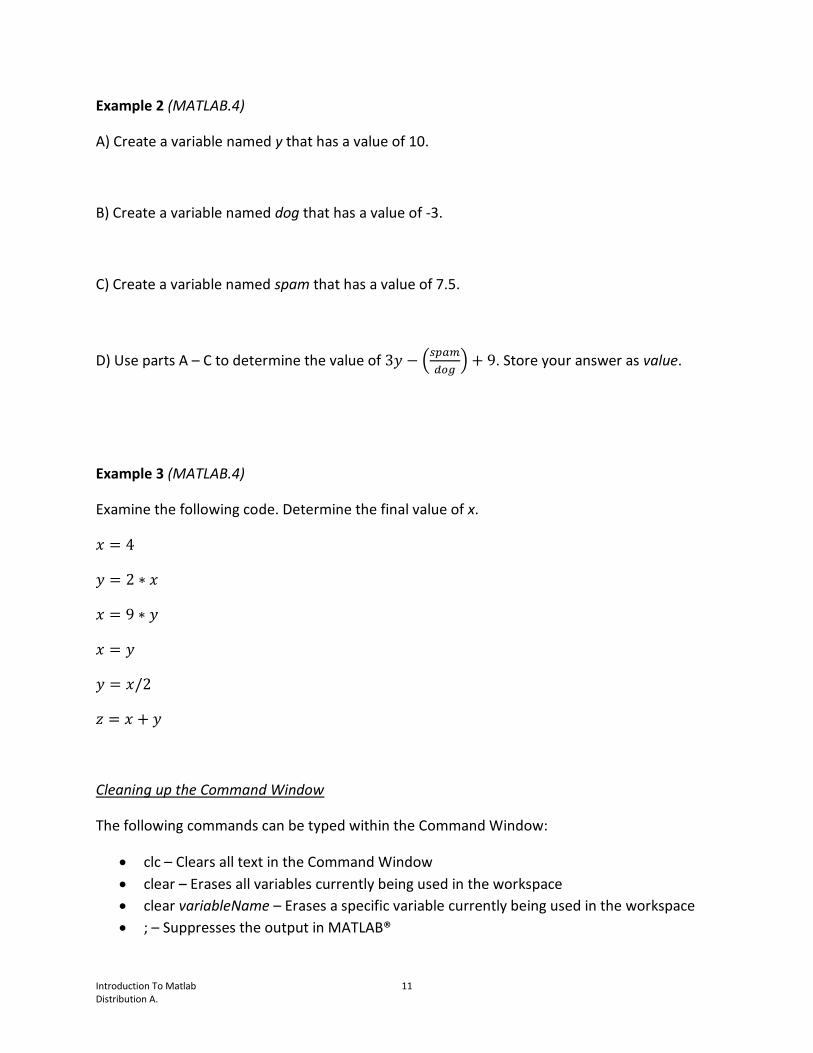
Example 2 (MATLAB.4)
A) Create a variable named y that has a value of 10.
B) Create a variable named dog that has a value of -3.
C) Create a variable named spam that has a value of 7.5.
D) Use parts A – C to determine the value of 3𝑦 − (𝑠𝑝𝑎𝑚
𝑑𝑜𝑔) + 9. Store your answer as value.
Example 3 (MATLAB.4)
Examine the following code. Determine the final value of x.
𝑥 = 4
𝑦 = 2 ∗ 𝑥
𝑥 = 9 ∗ 𝑦
𝑥 = 𝑦
𝑦 = 𝑥/2
𝑧 = 𝑥 + 𝑦
Cleaning up the Command Window
The following commands can be typed within the Command Window:
clc – Clears all text in the Command Window
clear – Erases all variables currently being used in the workspace
clear variableName – Erases a specific variable currently being used in the workspace
; – Suppresses the output in MATLAB®

Introduction To Matlab 12 Distribution A.
1.5. ASSESSMENT – PRACTICE PROBLEMS
Students should be able to complete the practice problems below to demonstrate their
understanding. Encourage students to refer to their notes, research online, or work together to
overcome any issues they may encounter. It is recommended that students receive a digital
version of these problems so that they can copy and paste their answers straight from
MATLAB®.
Practice Problems:
1) Use MATLAB® to perform each calculation. Be sure to use proper syntax and order of
operations.
A) 11(12 − 7)2 − 2(4) B) (21
7) (8) +
(2−5)2
9 C)
12(8−9)3+21
(−3−8)2
2) Write down the code that gives the variable Spam the value of 14.
3) If a = 15, b = -6, and c = 21, what is the value of 𝑎−𝑏
𝑐+ 3𝑐 − 𝑎𝑏2?
4) Examine the following code and determine the value of cat at the end.
𝑝𝑖𝑔 = 7
𝑑𝑜𝑔 = −5
𝑐𝑎𝑡 = 3
𝑝𝑖𝑔 = 𝑑𝑜𝑔 + 𝑐𝑎𝑡
𝑑𝑜𝑔 = 3 ∗ 𝑐𝑎𝑡 − 4 ∗ 𝑑𝑜𝑔
𝑐𝑎𝑡 = 3 + 𝑐𝑎𝑡 − 𝑑𝑜𝑔 ∗ 𝑝𝑖𝑔

Introduction To Matlab 13 Distribution A.
52 feet
120 feet
5) Use MATLAB® to calculate the volume of a cylinder that has a radius of 5 cm and a height of
24 cm. Be sure to write your code in the space below along with your answer.
NOTE: The formula for volume of a cylinder is 𝑉 = 𝜋𝑟2ℎ and to type 𝜋 into MATLAB® use the
keyword pi.
6) A person wants to do some landscaping in their backyard. They would like to fence in the
backyard as well as plant a new type of grass. An outline of the space is shown below. The
backyard is a rectangle and the fence will be installed along the border of the backyard.
The fence to be used costs $79.20 for an 8-foot long panel and must be purchased in whole
panels (cannot buy part of a panel). The grass seed is $13.39 for a 3-pound bag, and will cover
an area of about 1500 square feet.
Use MATLAB® and the above information to determine the total cost of landscaping the
backyard.
Break the Problem Down:
A) How much fence will be needed? Create a variable to store this information. Write your
code in the space below.

Introduction To Matlab 14 Distribution A.
B) How much grass seen will be needed? Create a variable to store this information. Write
your code in the space below. (HINT: How do you find the area of the shape?)
C) Use the information you found and the variables you created in A and B to determine
the total cost of the landscaping project.
1.6. ANSWER KEYS
1.6.1. GUIDED NOTES
Introduction to MATLAB®
Mathematics and Variables in MATLAB® (Part 1)
Name:___________________________ Date:_____________ Period:__________
Learning Targets:
MATLAB.1 – Be able to describe MATLAB and its general capabilities.
MATLAB.2 – Be able to identify the different parts of the MATLAB window and explain what
they do.
MATLAB.3 – Be able to perform basic mathematical operations in MATLAB.
MATLAB.4 – Be able to declare and use variables in MATLAB.
What is MATLAB? (MATLAB.1)
MATLAB (short for Matrix Laboratory) is a mathematical software package that is primarily used
for numerical COMPUTATION and data ANALYSIS along with various PROGRAMMING
capabilities.

Introduction To Matlab 15 Distribution A.
Figure 1: MATLAB Window. The MathWorks©, Inc.: MATLAB® version R2018a. Screenshot by author.
The MATLAB Window (MATLAB.2)
MATLAB Basics (MATLAB.3)
MATLAB can be used to perform various mathematical computations just like a calculator. Here
are some of the more commonly used mathematical operations (Table 1):
Operation Symbol
Addition +
Subtraction -
Multiplication *
Division /
Exponent/Power ^ Table 1: MATLAB Math Operations
Example 1 (MATLAB.3)
Use MATLAB to calculate each of the following. Be sure to use order of operations.
Current Folder –
SHOWS ALL
MATLAB FILES
CREATED IN
THE
WORKING
DIRECTORY
Editor –
SPACE USED TO WRITE
SCRIPTS/PROGRAMS
Command Window –
SPACE USED TO TEST COMMANDS
(EXECUTES ONE LINE AT A TIME).
OUTPUT OF A PROGRAM ALSO IS
DISPLAYED HERE.
Workspace –
SHOWS ALL
VARIABLES
CURRENTLY
IN USE
ALONG
WITH THEIR
VALUES

Introduction To Matlab 16 Distribution A.
A) 3(9 − 2)3 − 1234 B) 1804
4+ 80(7 − 10) C)
12+5(11+3)5
6(2−6)2
What are Variables in MATLAB? (MATLAB.4)
A variable in MATLAB (and other programming languages) is a letter or word used to STORE
data.
Declaring a variable means to assign a specific VALUE OR EXPRESSION to a variable.
Syntax: variableName = value/expression
Examples: 𝑥 = 5 𝑛𝑢𝑚𝑏𝑒𝑟 = 3 ∗ 𝑥 − 2
NOTE: Variable names must begin with a letter, and the variable name must be typed on the
left side of the “=” sign.
Example 2 (MATLAB.4)
A) Create a variable named y that has a value of 10.
y = 10
B) Create a variable named dog that has a value of -3.
dog = -3
C) Create a variable named spam that has a value of 7.5.
spam = 7.5
D) Use parts A – C to determine the value of 3𝑦 − (𝑠𝑝𝑎𝑚
𝑑𝑜𝑔) + 9. Store your answer as value.
value = 41.5

Introduction To Matlab 17 Distribution A.
Example 3 (MATLAB.4)
Examine the following code. Determine the final value of x.
𝑥 = 4
𝑦 = 2 ∗ 𝑥
𝑥 = 9 ∗ 𝑦
𝑥 = 𝑦
𝑦 = 𝑥/2
𝑧 = 𝑥 + 𝑦
Cleaning up the Command Window
The following commands can be typed within the Command Window:
clc – Clears all text in the Command Window
clear – Erases all variables currently being used in the workspace
clear variableName – Erases specific variable currently being used in the workspace
; – Suppresses the output in MATLAB
1.6.2. PRACTICE PROBLEMS
Practice Problems:
1) Use MATLAB to perform each calculation. Be sure to use proper syntax and order of
operations.
A) 11(12 − 7)2 − 2(4) B) (21
7) (8) +
(2−5)2
9 C)
12(8−9)3+21
(−3−8)2
x y z
4 - -
4 8 -
72 8 -
8 8 -
8 4 -
8 4 12

Introduction To Matlab 18 Distribution A.
2) Write down the code that gives the variable Spam the value of 14.
3) If a = 15, b = -6, and c = 21, what is the value of 𝑎−𝑏
𝑐+ 3𝑐 − 𝑎𝑏2?
4) Examine the following code and determine the value of cat at the end.
𝑝𝑖𝑔 = 7
𝑑𝑜𝑔 = −5
𝑐𝑎𝑡 = 3
𝑝𝑖𝑔 = 𝑑𝑜𝑔 + 𝑐𝑎𝑡
𝑑𝑜𝑔 = 3 ∗ 𝑐𝑎𝑡 − 4 ∗ 𝑑𝑜𝑔
𝑐𝑎𝑡 = 3 + 𝑐𝑎𝑡 − 𝑑𝑜𝑔 ∗ 𝑝𝑖𝑔
pig dog cat
7 - -
7 -5 -
7 -5 3
7 29 3
7 29 -197

Introduction To Matlab 19 Distribution A.
52 feet
120 feet
5) Use MATLAB to calculate the volume of a cylinder that has a radius of 5 cm and a height of
24 cm. Be sure to write your code in the space below, along with your answer.
NOTE: The formula for volume of a cylinder is 𝑉 = 𝜋𝑟2ℎ and to type 𝜋 into MATLAB use the
keyword pi.
or
6) A person wants to do some landscaping in their backyard. They would like to fence in the
backyard as well as plant a new type of grass. An outline of the space is shown below. The
backyard is a rectangle and the fence will be installed along the border of the backyard.
The fence to be used costs $79.20 for an 8-foot long panel and must be purchased in whole
panels (cannot buy part of a panel). The grass seed is $13.39 for a 3-pound bag, and will cover
an area of about 1500 square foot.
Use MATLAB and the above information to determine the total cost of landscaping the
backyard.
Break the Problem Down:

Introduction To Matlab 20 Distribution A.
A) How much fence will be needed? Create a variable to store this information. Write your
code in the space below.
First, students should find the perimeter of the yard by adding up all the side lengths.
This will give students the total number of feet of fence needed (344 feet), but since we
can only buy the fence in 8-ft panels, students will need to divide the perimeter by 8.
Students should find that 43 panels will need to be purchased.
B) How much grass seen will be needed? Create a variable to store this information. Write
your code in the space below. (HINT: How do you find the area of the shape?)
For this question, students will have to find the area of the backyard using the formula
𝐴𝑟𝑒𝑎 = 𝑙𝑒𝑛𝑔𝑡ℎ ∗ 𝑤𝑖𝑑𝑡ℎ, where the length is 120 feet and the width is 52 feet. Once
students have the area, they need to divide it by the number of square feet a bag of
grass seed will cover. This results in 4.16 bags needed; however, since we cannot
purchase part of a bag, 5 bags will be necessary to cover the backyard.
C) Use the information you found and the variables you created in A and B to determine
the total cost of the landscaping project.
The total cost for landscaping will be 3.4752e+03 which is scientific notation for: $3472.50
(The actual cost is $3472.55, but gets truncated due to MATLAB’s formatting)

Introduction To Matlab 21 Distribution A.
NOTE: If students do some research, they should be able to find a way to have the answer
display in a different notation. One way is to type the words format long g into the command
window and press enter. This will re-format all answers in the command window until the
format is changed or MATLAB is closed.
1.7. RESOURCES
1. The MathWorks©, Inc./MATLAB® Official Support Page:
https://www.mathworks.com/help/matlab/

Introduction To Matlab 22 Distribution A.
MATHEMATICS AND VARIABLES IN MATLAB ® (PART 2)
1.8. INTRODUCTION
In this lesson, students will work with trigonometry and coordinate geometry. Specifically,
students will learn how to use sine, cosine, tangent, and square roots in MATLAB®.
1.9. MATERIALS
Each student will need:
PC/Mac with MATLAB® installed
Copy of Introduction to MATLAB® - Mathematics and Variables in MATLAB® (Part 2)
guided notes (these may be printed or shared digitally):
https://padlet.com/abrumbaugh/introMatlab
The teacher will need:
PC/MAC with MATLAB® installed
Ceiling projector or method of displaying their computer screen for students to see
Copy of Introduction to MATLAB® - Mathematics and Variables in MATLAB® (Part 2)
answer key
1.10. OVERVIEW OF PLAN
This lesson can be taught via direct instruction or student-paced learning through online videos
located at https://padlet.com/abrumbaugh/introMatlab.
1.10.1. LEARNING TARGET – MATLAB.5
Be able to perform advanced mathematical calculations with MATLAB®.
By the end of this lesson, students should feel comfortable entering more advanced commands
for more complicated calculations in MATLAB®. Students should also be aware that there are
many more computations that MATLAB® can perform. A large list of these different options is
located at https://www.mathworks.com/help/symbolic/mathematical-functions.html.
With this lesson focusing heavily on trigonometry, have students pay close attention to the
units used for angle measurements in these problems. A problem with angle measurements in
degrees will have a different syntax than a problem with angle measurements in radians.

Introduction To Matlab 23 Distribution A.
Furthermore, make sure students are using parentheses wisely and following order of
operations.
1.11. GUIDED NOTES
Introduction to MATLAB®
Mathematics and Variables in MATLAB® (Part 2)
Name:___________________________ Date:_____________ Period:__________
Learning Targets:
MATLAB.5 – Be able to perform advanced mathematical calculations with MATLAB®.
Advanced Mathematics in MATLAB® (MATLAB.5)
MATLAB® can perform more than just basic mathematical operations (e.g., addition,
subtraction). MATLAB® has access to many different mathematical functions that can be used
in a variety of situations. For a list of these functions, see
https://www.mathworks.com/help/symbolic/mathematical-functions.html.
Right Triangle Trigonometry Review
Trigonometry is a branch of mathematics that studies the sides and angles of a triangle and the
relationships between them. Recall from math class, for any right triangle (i.e., a triangle that
contains a 90° angle), the following ratios are true.
Sine: Cosine: Tangent:
sin(𝜃) = cos(𝜃) = tan(𝜃) =
To remember the trigonometric ratios:
Hypotenuse
θ
Opposite
Adjacent

Introduction To Matlab 24 Distribution A.
sin(𝐴) = sin(𝐵) =
cos(𝐴) = cos(𝐵) =
tan(𝐴) = tan(𝐵) =
Syntax for Trigonometric Functions in MATLAB®
Trigonometric Function Angle Measured in DEGREES
Angle Measured in RADIANS
Sine sind(angle_measure) sin(angle_measure)
Cosine cosd(angle_measure) cos(angle_measure)
Tangent tand(angle_measure) tan(angle_measure) Figure 2: Trigonometric Functions in MATLAB®
NOTE: Be sure to identify whether a given problem measures angles in degrees or radians, as
the syntax for each trigonometric ratio changes.
Example 1 (MATLAB.5)
Use MATLAB® to find the missing side lengths of the triangle. Be sure to write the code you
used to find your answers.
20°
30 ft
x
y
a
c
B
A C b

Introduction To Matlab 25 Distribution A.
Example 2 (MATLAB.5)
Use MATLAB® to solve the following:
From a point on the ground 47 feet from the foot of a tree, the angle of elevation of the
top of the tree is 35°. Find the height of the tree and write the code you used to find
your answer.
Example 3 (MATLAB.5)
Use MATLAB® to solve the following:
To take the square root of a number in MATLAB®, use the command sqrt(number). Use the
Pythagorean Theorem (𝑎2 + 𝑏2 = 𝑐2) to determine the missing side length of each triangle in
MATLAB®.
A) B)
6 cm
10 cm
x
25 cm
21 cm
x

Introduction To Matlab 26 Distribution A.
Example 4 (MATLAB.5)
Use MATLAB® to solve the following:
The distance formula can be used to find the distance between two points on a coordinate
plane. The distance formula is 𝑑 = √(𝑥2 − 𝑥1)2 + (𝑦2 − 𝑦1)2. Use this formula to find the
distance between the given points.
A) (2, 3) (−3, 10) B) (−7.5, 10) (11,−22)
1.12. ASSESSMENT – PRACTICE PROBLEMS
Students should be able to complete the practice problems below to demonstrate their
understanding. Encourage students to refer to their notes, research online, or work together to
overcome any issues they may encounter. It is recommended that students receive a digital
version of these problems so that they can copy and paste their answers straight from
MATLAB®.
Practice Problems:
1) Use MATLAB® to find the missing side lengths of the triangle. Be sure to write the code you
used to find your answers.
x
55°
12 m y

Introduction To Matlab 27 Distribution A.
2) Use MATLAB® to solve the following:
You are watching an airplane. The angle of elevation of the airplane is about 23°. If the
airplane’s altitude (height) is 2500 meters, how far away are you from the airplane?
3) Use MATLAB® to find the missing side length of each triangle.
A) B)
4) Use MATLAB® to find the distance between each pair of points.
A) (−12, 16) (7, 18) B) (12.8, 9) (−5,−7.2)
5 ft
12 ft
x 38 ft
x
17 ft

Introduction To Matlab 28 Distribution A.
1.13. ANSWER KEYS
1.13.1. GUIDED NOTES
Introduction to MATLAB®
Mathematics and Variables in MATLAB® (Part 2)
Name:___________________________ Date:_____________ Period:__________
Learning Targets:
MATLAB.5 – Be able to perform advanced mathematical calculations with MATLAB®.
Advanced Mathematics in MATLAB® (MATLAB.5)
MATLAB® can perform more than just basic mathematical operations (e.g., addition,
subtraction). MATLAB® has access to many different mathematical functions that can be used
in a variety of situations. For a list of these functions, see
https://www.mathworks.com/help/symbolic/mathematical-functions.html.
Right Triangle Trigonometry Review
Trigonometry is a branch of mathematics that studies the sides and angles of a triangle and the
relationships between them. Recall from math class, for any right triangle (i.e., a triangle that
contains a 90° angle), the following ratios are true.
Sine: Cosine: Tangent:
sin(𝜃) = 𝑂𝑝𝑝𝑜𝑠𝑖𝑡𝑒
𝐻𝑦𝑝𝑜𝑡𝑒𝑛𝑢𝑠𝑒 cos(𝜃) =
𝐴𝑑𝑗𝑎𝑐𝑒𝑛𝑡
𝐻𝑦𝑝𝑜𝑡𝑒𝑛𝑢𝑠𝑒 tan(𝜃) =
𝑂𝑝𝑝𝑜𝑠𝑖𝑡𝑒
𝐴𝑑𝑗𝑎𝑐𝑒𝑛𝑡
To remember the trigonometric ratios: 𝑆𝑂𝐻 − 𝐶𝐴𝐻 − 𝑇𝑂𝐴
sin(𝐴) =𝑎
𝑐 sin(𝐵) =
𝑏
𝑐
cos(𝐴) = 𝑏
𝑐 cos(𝐵) =
𝑎
𝑐
tan(𝐴) =𝑎
𝑏 tan(𝐵) =
𝑏
𝑎
Hypotenuse
θ
Opposite
Adjacent
a
c
B
A C b

Introduction To Matlab 29 Distribution A.
Syntax for Trigonometric Functions in MATLAB®
Trigonometric Function Angle Measured in DEGREES
Angle Measured in RADIANS
Sine sind(angle_measure) sin(angle_measure)
Cosine cosd(angle_measure) cos(angle_measure)
Tangent tand(angle_measure) tan(angle_measure) Figure 2: Trigonometric Functions in MATLAB®
NOTE: Be sure to identify whether a given problem measures angles in degrees or radians, as
the syntax for each trigonometric ratio changes.
Example 1 (MATLAB.5)
Use MATLAB® to find the missing side lengths of the triangle. Be sure to write the code you
used to find your answers.
Example 2 (MATLAB.5)
Use MATLAB® to solve the following:
From a point on the ground 47 feet from the foot of a tree, the angle of elevation of the top of
the tree is 35°. Find the height of the tree and write the code you used to find your answer.
20°
30 ft
x
y

Introduction To Matlab 30 Distribution A.
Example 3 (MATLAB.5)
Use MATLAB® to solve the following:
To take the square root of a number in MATLAB, use the command sqrt(number). Use the
Pythagorean Theorem (𝑎2 + 𝑏2 = 𝑐2) to determine the missing side length of each triangle in
MATLAB®.
A) B)
Example 4 (MATLAB.5)
Use MATLAB® to solve the following:
The distance formula can be used to find the distance between two points on a coordinate
plane. The distance formula is 𝑑 = √(𝑥2 − 𝑥1)2 + (𝑦2 − 𝑦1)2. Use this formula to find the
distance between the given points.
A) (2, 3) (−3, 10) B) (−7.5, 10) (11,−22)
6 cm
10 cm
x
25 cm
21 cm
x

Introduction To Matlab 31 Distribution A.
1.13.2. PRACTICE PROBLEMS
Practice Problems:
1) Use MATLAB® to find the missing side lengths of the triangle. Be sure to write the code you
used to find your answers.
2) Use MATLAB® to solve the following:
You are watching an airplane. The angle of elevation of the airplane is about 23°. If the
airplane’s altitude (height) is 2500 meters, how far away are you from the airplane?
3) Use MATLAB® to find the missing side length of each triangle.
A) B)
x
55°
12 m y
5 ft
12 ft
x 38 ft
x
17 ft

Introduction To Matlab 32 Distribution A.
4) Use MATLAB® to find the distance between each pair of points.
A) (−12, 16) (7, 18) B) (12.8, 9) (−5,−7.2)
1.14. RESOURCES
1. The MathWorks©, Inc./MATLAB® Official Support Page:
https://www.mathworks.com/help/matlab/
2. MATLAB® Mathematical Functions:
https://www.mathworks.com/help/symbolic/mathematical-functions.html

Introduction To Matlab 33 Distribution A.
CREATING SCRIPTS IN MATLAB®
1.15. INTRODUCTION
In this lesson students will learn how to work with the editor in MATLAB® to create scripts, use
scripts to solve a variety of mathematical problems, and learn how to use the input function.
1.16. MATERIALS
Each student will need:
PC/Mac with MATLAB® installed
Copy of Introduction to MATLAB® - Creating Scripts in MATLAB® guided notes (these
may be printed or shared digitally): https://padlet.com/abrumbaugh/introMatlab
The teacher will need:
PC/MAC with MATLAB® installed
Ceiling projector or way to display their computer screen for students to see
Copy of Introduction to MATLAB® - Creating Scripts in MATLAB® answer key
1.17. OVERVIEW OF PLAN
This lesson can be taught via direct instruction or student-paced learning through online videos
located at https://padlet.com/abrumbaugh/introMatlab.
1.17.1. LEARNING TARGET – MATLAB.6
Be able to explain what a script is in MATLAB®
A script is MATLAB®’s version of a program. Students should understand that scripts are a series
of lines of code that are entered into the editor window. These lines of code will run in order
from top to bottom once the Run button, represented by the green arrow, is pressed. Scripts
are very useful for automating several calculations or commands at one time.
1.17.2. LEARNING TARGET – MATLAB.7
Be able to create scripts that model and solve simple mathematical problems.
Building on the work completed in the first two lessons, students will apply their ability to do
mathematics in MATLAB® with scripting. Students will utilize the MATLAB® editor to create
scripts that take a set of variables and perform various calculations with them. Students should

Introduction To Matlab 34 Distribution A.
see how creating a script for a set of problems is more efficient than repeatedly using the
command window for each individual problem.
1.17.3. LEARNING TARGET – MATLAB.8
Be able to use the input function within scripts in MATLAB®
This is the first non-mathematical function that students will learn how to use in MATLAB®. The
input function has the ability to take a value that has been entered by a user running the
program and store it within a specified variable. The input function also allows programmers to
display a prompt that informs the user as to what information they should type in. Encourage
students to write clear and concise prompts when using the input function.
The input function allows users to type in numbers/scalars, matrices and arrays, as well as
strings. Depending on the type of information that is to be entered, the input function syntax
will change slightly. If the program is expecting a numeric answer, whether it is a single number
(scalar) or matrix (a rectangular array of numbers), the syntax will be variableName =
input(‘Prompt’). If the program is expecting a string, such as a person’s name, the syntax will be
variableName = input(‘Prompt’,’s’).
1.18. GUIDED NOTES
Introduction to MATLAB®
Creating Scripts in MATLAB®
Name:___________________________ Date:_____________ Period:__________
Learning Targets:
MATLAB.6 – Be able to explain what a script is in MATLAB®.
MATLAB.7 – Be able to create scripts that model and solve simple mathematical problems.
MATLAB.8 – Be able to use the input function within scripts in MATLAB®.
Scripts in MATLAB® (MATLAB.6)
In MATLAB®, a script is a sequence of __________ that executes one line at a time from the top
down.

Introduction To Matlab 35 Distribution A.
Figure 2: New Script Button. The MathWorks©,Inc.: MATLAB© R2018a. Screenshot by author.
Figure 3: Run Button. The MathWorks©,Inc.: MATLAB© R2018a. Screenshot by author.
Scripts are useful in MATLAB® as they can _________________ many tasks such as
mathematical calculations.
Scripts are created in the ___________________ window and are saved as the ____________
file type.
Automating Calculations Using Scripts (MATLAB.7)
To create a new script in MATLAB®, click the New Script button
(see Figure 2)
on the HOME tab. This will open up the Editor window where the
code will be typed.
You might notice that pressing Enter after typing a
line of code in the Editor window does not run any
code, and instead, moves the cursor down to the
next line of the Editor window. This is because the
Editor will run all of the code only when the Run
button (see Figure 3) is selected from the EDITOR
tab.
Example 1 (MATLAB.7)
A) Create a script that takes two variable values, a and b, and finds the difference of the two
numbers. Write the lines of code in the space below.
B) Create a script that calculates the area of a triangle. Write the lines of code in the space
below.

Introduction To Matlab 36 Distribution A.
C) Create a script that finds the hypotenuse of a right triangle using the Pythagorean Theorem
(𝑎2 + 𝑏2 = 𝑐2). Write the lines of code in the space below.
Data Types
MATLAB®, as well as other programming languages, uses two primary types of data: numeric
and string. There are many different types of numeric data (e.g., integer, float), and they are
composed of numbers. The string data type is a value that is a letter, character, or combination
of letters and characters. It is important to have a basic understanding and awareness of data
types as many of the built-in functions of MATLAB® require a specific data type.
Input Function
The input function is a built-in function of MATLAB® that allows a program to get information
from a user (e.g., measurements, name). Depending on the data type that is to be entered (i.e.,
numeric or string), the syntax for input varies (Table 2):
Numeric Input String Input
Syntax variableName = input(‘Prompt’) variableName = input(‘Prompt’,’s’)
Example length = input(‘What is the length?’) name = input(‘What is your name?’,’s’)
Table 2: Input Syntax
*NOTE: For both input types, the prompt (i.e., the words that will be displayed) must be in
single quotes.
Example 2 (MATLAB.8)
A) Create a script that has the user enter the radius and height of a cylinder, and then uses
those values to calculate the volume of the cylinder.

Introduction To Matlab 37 Distribution A.
B) Use your script to find the volume of a cylinder with radius 10 cm and height 25 cm.
Example 3 (MATLAB.8)
A) Create a script that calculates a user’s gross pay (i.e., amount made before taxes are taken
out) based on their hourly wage, number of hours they worked, and any tips/commission they
may have made during the week.
B) Use your script to find the gross pay of someone who makes $6.75 per hour, worked for 35
hours, and made $257.50 in tips.
1.19. ASSESSMENT – PRACTICE PROBLEMS
Students should be able to complete the practice problems below to demonstrate their
understanding. Encourage students to refer to their notes, research online, or work together to
overcome any issues they may encounter. It is recommended that students receive a digital
version of these problems so that they can copy and paste their answers straight from
MATLAB®.
Practice Problems:
1) The area of a trapezoid is found by taking ½ the sum of the two bases multiplied by the
height of the trapezoid, or 𝐴 =1
2(𝑏1 + 𝑏2)ℎ.
Base 1 (𝑏1)
Base 2 (𝑏2)
Height

Introduction To Matlab 38 Distribution A.
A) Create a script in MATLAB® that will calculate the area of a trapezoid. Write your script
in the space below.
B) Use your script to find the areas of the following trapezoids.
Area:_______________ Area:_______________
2) Radio antennas are supported by long cables to keep them from toppling. Write a script that
takes the angle the cable makes with the ground and the distance of the cable attachment from
the base of the tower and finds the height of the tower AND length of the cable. (HINT: You will
need to use trigonometry.)
Script:
Check your script with the following test cases:
A) 25 feet, 30 degrees
8 m
15 m
10 m
221 ft
445 ft
250 ft

Introduction To Matlab 39 Distribution A.
B) 100 feet, 60 degrees
3) Banks offer savings, checking, and investment plans that gain compound interest. To
determine the amount of money in one of these accounts, the formula, 𝐴 = 𝑃 (1 +𝑟
𝑛)𝑛𝑡
, can
be used. In this formula, 𝐴 is the amount of money in the account, 𝑃 is the principal/starting
amount of money in the account, 𝑟 is the interest rate as a decimal (e.g., 3% = 0.03, 2.5% =
0.025, 15.3% = 0.153), 𝑛 is the number of compounding periods in one year, and 𝑡 is the time in
years.
Create a script that will calculate the value of 𝐴 given 𝑃, 𝑟, 𝑛, and 𝑡. Use the script to complete
the table below.
Script:
Starting Amount
(P)
Rate
(r)
# of Compounds per Year
(n)
Time
(t)
Final Amount
(A)
$1,000 5% 4 10 years
$5,000 3.4% 12 15 years
$12,550 4.35% 26 25 years
1.20. ANSWER KEYS

Introduction To Matlab 40 Distribution A.
Figure 2: New Script Button. . The MathWorks©,Inc.: MATLAB© R2018a. Screenshot by author.
Figure 3: Run Button. The MathWorks©,Inc.: MATLAB© R2018a. Screenshot by author.
1.20.1. GUIDED NOTES
Introduction to MATLAB®
Creating Scripts in MATLAB®
Name:___________________________ Date:_____________ Period:__________
Learning Targets:
MATLAB.6 – Be able to explain what a script is in MATLAB®.
MATLAB.7 – Be able to create scripts that model and solve simple mathematical problems.
MATLAB.8 – Be able to use the input function within scripts in MATLAB®.
Scripts in MATLAB® (MATLAB.6)
In MATLAB®, a script is a sequence of CODE that executes one line at a time from the top down.
Scripts are useful in MATLAB® as they can AUTOMATE many tasks such as mathematical
calculations.
Scripts are created in the EDITOR window and are saved as the .M file type.
Automating Calculations Using Scripts (MATLAB.7)
To create a new script in MATLAB®, click the New Script button
(see Figure 2)
on the HOME tab. This will open up the Editor window where the
code will be typed.
You might notice that pressing Enter after typing a
line of code in the Editor window does not run any
code, and instead, moves the cursor down to the
next line of the Editor window. This is because the
Editor will run all of the code only when the Run
button (see Figure 3) is selected from the EDITOR

Introduction To Matlab 41 Distribution A.
tab.
Example 1 (MATLAB.7)
A) Create a script that takes two variable values, a and b, and finds the difference of the two
numbers. Write the lines of code in the space below.
B) Create a script that calculates the area of a triangle. Write the lines of code in the space
below.
C) Create a script that finds the hypotenuse of a right triangle using the Pythagorean Theorem
(𝑎2 + 𝑏2 = 𝑐2). Write the lines of code in the space below.
Data Types
MATLAB®, as well as other programming languages, uses two primary types of data: numeric
and string. There are many different types of numeric data (e.g., integer, float), and they are
composed of numbers. The string data type is a value that is a letter, character, or combination
of letters and characters. It is important to have a basic understanding and awareness of data
types as many of the built-in functions of MATLAB® require a specific data type.

Introduction To Matlab 42 Distribution A.
Input Function
The input function is a built-in function of MATLAB® that allows a program to get information
from a user (e.g., measurements, name). Depending on the data type that is to be entered (i.e.,
numeric or string), the syntax for input varies (Table 2):
Numeric Input String Input
Syntax variableName = input(‘Prompt’) variableName = input(‘Prompt’,’s’)
Example length = input(‘What is the length?’) name = input(‘What is your name?’,’s’)
Table 2: Input Syntax
*NOTE: For both input types, the prompt (i.e., the words that will be displayed) must be in
single quotes.
Example 2 (MATLAB.8)
A) Create a script that has the user enter the radius and height of a cylinder, and then uses
those values to calculate the volume of the cylinder.
B) Use your script to find the volume of a cylinder with radius 10 cm and height 25 cm.
Example 3 (MATLAB.8)

Introduction To Matlab 43 Distribution A.
A) Create a script that calculates a user’s gross pay (i.e., amount made before taxes are taken
out) based on their hourly wage, number of hours they worked, and any tips/commission they
may have made during the week.
B) Use your script to find the gross pay of someone who makes $6.75 per hour, worked for 35
hours, and made $257.50 in tips.
1.20.2. PRACTICE PROBLEMS
Practice Problems:
1) The area of a trapezoid is found by taking ½ the sum of the two bases multiplied by the
height of the trapezoid, or 𝐴 =1
2(𝑏1 + 𝑏2)ℎ.
A) Create a script in MATLAB® that will calculate the area of a trapezoid. Write your script
in the space below.
B) Use your script to find the areas of the following trapezoids.
Area: 15 𝑚2 Area: 83250 𝑓𝑡2
Base 1 (𝑏1)
Base 2 (𝑏2)
Height
8 m
15 m
10 m
221 ft
445 ft
250 ft

Introduction To Matlab 44 Distribution A.
2) Radio antennas are supported by long cables to keep them from toppling. Write a script that
takes the angle the cable makes with the ground and the distance of the cable attachment from
the base of the tower and finds the height of the tower AND length of the cable. (HINT: You will
need to use trigonometry.)
Script:
Check your script with the following test cases:
A) 25 feet, 30 degrees
B) 100 feet, 60 degrees

Introduction To Matlab 45 Distribution A.
3) Banks offer savings, checking, and investment plans that gain compound interest. To
determine the amount of money in one of these accounts, the formula, 𝐴 = 𝑃 (1 +𝑟
𝑛)𝑛𝑡
, can
be used. In this formula, 𝐴 is the amount of money in the account, 𝑃 is the principal/starting
amount of money in the account, 𝑟 is the interest rate as a decimal (e.g., 3% = 0.03, 2.5% =
0.025, 15.3% = 0.153), 𝑛 is the number of compounding periods in one year, and 𝑡 is the time in
years.
Create a script that will calculate the value of 𝐴 given 𝑃, 𝑟, 𝑛, and 𝑡. Use the script to complete
the table below.
Script:
Starting Amount
(P)
Rate
(r)
# of Compounds per Year
(n)
Time
(t)
Final Amount
(A)
$1,000 5% 4 10 years $1,643.62
$5,000 3.4% 12 15 years $8,320.45
$12,550 4.35% 26 25 years $37,200.12

Introduction To Matlab 46 Distribution A.
1.21. RESOURCES
1. The MathWorks©, Inc./MATLAB® Official Support Page:
https://www.mathworks.com/help/matlab/
2. MATLAB® Onramp Tutorial: https://matlabacademy.mathworks.com/

Introduction To Matlab 47 Distribution A.
COMMENTS AND FORMATTING STRINGS
1.22. INTRODUCTION
In this lesson, students will learn about the importance of comments within code and how
comments can be created in MATLAB®. Students will also learn how to format the output of a
script using the fprintf function and new line switch.
1.23. MATERIALS
Each student will need:
PC/Mac with MATLAB® installed
Copy of Introduction to MATLAB® - Comments and Formatting Strings guided notes
(these may be printed or shared digitally): https://padlet.com/abrumbaugh/introMatlab
The teacher will need:
PC/MAC with MATLAB® installed
Ceiling projector or way to display their computer screen for students to see
Copy of Introduction to MATLAB® - Comments and Formatting Strings answer key
1.24. OVERVIEW OF PLAN
This lesson can be taught via direct instruction or student-paced learning through online videos
located at https://padlet.com/abrumbaugh/introMatlab.
1.24.1. LEARNING TARGET – MATLAB.9
Be able to use comments to annotate code within a program/script.
One important feature of MATLAB® and many other programming languages is the ability to
add comments to code. Comments allow programmers to annotate their code making it more
readable by others who may not be familiar with the programming language. Comments can be
used as a resource to the programmer as they may need to look back at a program they created
earlier to review/re-learn how they completed a certain task. Comments can act as pseudocode
that explains the intention of how certain parts of a program are supposed to work. Students
should begin developing good programming habits throughout this unit, and leaving comments
in code is one them.

Introduction To Matlab 48 Distribution A.
The percent sign (%) is used to leave a comment in MATLAB®. When MATLAB® encounters a %,
it interprets the symbol and all characters immediately following it as a comment. The
computer does not run this code, but rather skips over it. MATLAB® color codes comments in a
green font.
1.24.2. LEARNING TARGET – MATLAB.10
Be able to use the fprintf function to format outputs that contain strings.
To make the output of a script easier to read and/or understand, students can utilize the fprintf
function. This function allows students to incorporate a string (e.g., sentence, word) with a
numeric output. For instance, a student may write a program that calculates the distance
between two objects. Typically, MATLAB® will display a single number as the output; however,
with the fprintf function, students will be able to add a unit to this answer (e.g., 5 feet) or place
the answer in a sentence (e.g., “The distance between the two poles is 5 feet.”) This formatting
option is beneficial as it clearly states what the output represents and can make it much easier
for non-programmers to use and interpret the work done by the script.
The syntax for the fprintf function may be intimidating for some students. The syntax is as
follows:
fprintf(‘Text to be displayed %specifier.’, variableName)
The function works similarly to the input function covered in the previous lesson. After the
keyword fprintf, students will type a sentence or word within single quotes between the
parentheses. To insert a variable’s value/output in the sentence, a specifier must be typed
where the value is supposed to appear within the sentence. Students can then type a comma
after the single quotes and type the name of the variable(s) that should be inserted into the
sentence. It is possible for students to use multiple specifiers in a sentence as long as the
number of variables is equal to the number of specifiers.
There are several specifier types, but each begin with the percent sign (%). Students should
take care when determining the specifier type to use (e.g., “Should the answer have a decimal?
Does the answer contain letters or only numbers?”). A table of specifier types is listed in the
guided notes.
1.25. GUIDED NOTES
Introduction to MATLAB®
Comments and Formatting Strings

Introduction To Matlab 49 Distribution A.
Figure 4: Comments. The MathWorks©,Inc.: MATLAB© R2018a. Screenshot by author.
Name:___________________________ Date:_____________ Period:__________
Learning Targets:
MATLAB.9 – Be able to use comments to annotate code within a program/script.
MATLAB.10 – Be able to use the fprintf function to format outputs that contain strings.
Making Comments within a Program (MATLAB.9)
Most programming languages have a feature that allows users to create comments within their
code. The computer skips over lines that are comments and does not read/run them.
Comments can be created by placing a __________________ anywhere in a program file (e.g.,
on its own line, at the end of a line.) The green text in Figure 4 are comments.
Example
It is good practice to add comments that describe the code you have written. Here are some
reasons why comments are beneficial when programming:
Helps __________________________________ understand what a program does or is
supposed to do
Can act as a ________________________ for a programmer
Can be used as a form of _________________________ which explains what a program
does in coding language
Can be used to document _____________________ that were used when creating the
program
Example 1 (MATLAB.9)

Introduction To Matlab 50 Distribution A.
Figure 5: Formatting with fprintf. The MathWorks©,Inc.: MATLAB© R2018a. Screenshot by author.
Use MATLAB® to create a script that calculates the area of a circle after the user gives a radius
for the circle. Create at least two comments throughout the code explaining what it does, and
use the script to answer the two test cases.
Script with Comments:
Test Cases: A) radius = 12 inches area = B) radius = 20𝜋 cm area =
Formatting Strings (MATLAB.10)
In MATLAB®, we can format our outputs (i.e., what is printed to the screen) in a way that is
more meaningful and easier to understand. One way to do this is to use the fprintf( ) function
(see Figure 5). This function will allow us to take an answer we get from a calculation and
display it within a sentence.
This function contains several fields that can be filled in, but we will focus only on a few of
these fields for now. The simplified syntax is:
Syntax: fprintf(‘Text to be displayed %specifier’, variableName)
Example:
NOTE: The “%” is NOT treated as a comment when used within the fprintf( ) function. Instead, it
is used to tell MATLAB® where you would like a variable value to be placed (i.e., the specifier).

Introduction To Matlab 51 Distribution A.
In this example, %.2f is a specifier/place holder for the variable pay. The .2 tells MATLAB® to
round the value to two decimal places, and the f tells MATLAB® that the value should be of type
float (i.e., a number that contains decimals.)
Here is a list (Table 3) of commonly used formatting specifiers for the fprintf( ) function:
Specifier Description
%s Prints a string
%c Prints a single character
%d Prints an integer (no decimal)
%f Prints a floating point number (decimal) Table 3: Specifiers for fprintf
NOTE: You can place a period/decimal point and value between the % and f to specify the
number of decimal points a float should contain when being formatted with fprintf( ).
Example 2 (MATLAB.9, 10)
Pizza Shack is offering a special price on their pizzas for their 25-year anniversary. A customer
can get any large two-topping pizza for $6.99 and any large specialty pizza for $9.99. Pizza
Shack will also deliver your order to you for $1.50.
Use MATLAB® to create a script that allows a customer to specify the number of each type of
pizza they would like, calculates their total, and then applies a 7.5% tax and delivery fee. The
script should then only display the total amount that the customer owes for their order in a
well-formatted sentence.
Test your script by calculating the total cost of an order for 3 two-topping pizzas and 2 specialty
pizzas.

Introduction To Matlab 52 Distribution A.
Figure 6: NO New Line Switch. The MathWorks©,Inc.: MATLAB© R2018a. Screenshot
by author.
Figure 9: New Line Switch. The MathWorks©,Inc.: MATLAB© R2018a.
Screenshot by author.
Figure 10: Multiple New Line Switches. The MathWorks©,Inc.: MATLAB© R2018a. Screenshot
by author.
Figure 11: NO New Line Switch with Input Function. The MathWorks©,Inc.: MATLAB© R2018a. Screenshot by
author.
Figure 12: New Line Switch with Input Function. The MathWorks©,Inc.: MATLAB© R2018a. Screenshot by
author.
New Line Switch
The new line switch is another way that we can format our output. The new line switch will
display text or input field on the next line. This can be useful in making scripts/programs more
user-friendly and easier to read.
Syntax: fprintf(‘Text to be displayed \n’) input(‘Text to be displayed \n’)
Note: \n will only be interpreted as a new line switch when it is a part of fprintf( ), input( ), or
other MATLAB® functions.
Examples:
Example 3
Create a script in MATLAB® utilizing the new line switch command to write each word of the
sentence, “The quick brown fox jumps over the lazy dog.” on its own line.
Script:

Introduction To Matlab 53 Distribution A.
1.26. ASSESSMENT – PRACTICE PROBLEMS
Students should be able to complete the practice problems below to demonstrate their
understanding. Encourage students to refer to their notes, research online, or work together to
overcome any issues they may encounter. It is recommended that students receive a digital
version of these problems so that they can copy and paste their answers straight from
MATLAB®.
Practice Problems:
From this lesson forward, all scripts/programs should contain some comments that annotate
what it should do when executed.
1) Use MATLAB® to create a script that calculates the gross pay of an individual after they have
typed in their hourly wage, number of hours worked, and tips/commission made during the
week. Then calculate the individual’s net pay (i.e., gross income minus taxes) by removing 15%
of their gross income for taxes.
The program should only display the amount that was withheld for taxes and the individual’s
net pay in well-formatted sentences (e.g., “A total of $150 was withheld for taxes.” “Your net
pay is $850.”)
Script:
Use your script to calculate the following test cases:
A) Darryl makes $15.75 each hour as a sales associate at a major appliance store. Last week, he
worked 37 hours and made $288 in commission.
Taxes:_______________________ Net Pay:_______________________

Introduction To Matlab 54 Distribution A.
B) Ramya earns $6.89 each hour as a waitress. Last week, she worked for 40 hours and made
$521.27 in tips.
Taxes:_______________________ Net Pay:_______________________
C) Ja’son earns $14.35 per hour as an automotive sales representative. Last week, he worked 30
hours and made $537.50 in commission.
Taxes:_______________________ Net Pay:_______________________
2) For a projectile fired across a flat plane (i.e., two dimensional), the equations of motion that
can be used to find the time the projectile is in the air and the distance it has traveled are:
𝑡𝑖𝑚𝑒 =2∗velocity∗sin(𝑎𝑛𝑔𝑙𝑒)
𝑔 𝑑𝑖𝑠𝑡𝑎𝑛𝑐𝑒 = 𝑡𝑖𝑚𝑒 ∗ 𝑣𝑒𝑙𝑜𝑐𝑖𝑡𝑦 ∗ cos (𝑎𝑛𝑔𝑙𝑒).
NOTE: “Velocity” refers to the initial/starting velocity of the projectile, the “angle” is the angle
of launch from the horizontal axis, and “g” is the acceleration due to gravity (in this problem
𝑔 = 9.81 𝑚/𝑠2).
Create a script that takes the initial velocity, and angle of the projectile and returns the travel
time and landing distance in a well-formatted sentence (must be a single sentence that contains
both values).
Script:

Introduction To Matlab 55 Distribution A.
Use your script to calculate the following test cases:
A) Velocity = 100 m/s Angle = 30°
Time = _____________ Distance = _______________
B) Velocity = 25 m/s Angle = 10°
Time = _____________ Distance = _______________
C) Velocity = 30 m/s Angle = 70°
Time = _____________ Distance = _______________
3) Create a script in MATLAB® that will recreate the text seen below.
Script:
Learning MATLAB
can
be difficult
but
fun
1.27. ANSWER KEYS
1.27.1. GUIDED NOTES
Introduction to MATLAB®

Introduction To Matlab 56 Distribution A.
Figure 6: Comments. The MathWorks©,Inc.: MATLAB© R2018a. Screenshot by author.
Comments and Formatting Strings
Name:___________________________ Date:_____________ Period:__________
Learning Targets:
MATLAB.9 – Be able to use comments to annotate code within a program/script.
MATLAB.10 – Be able to use the fprintf function to format outputs that contain strings.
Making Comments within a Program (MATLAB.9)
Most programming languages have a feature that allows users to create comments within their
code. The computer skips over lines that are comments and does not read/run them.
Comments can be created by placing a ____%____ anywhere in a program file (e.g., on its own
line, at the end of a line.) The green text in Figure 4 are comments.
Example
It is good practice to add comments that describe the code you have written. Here are some
reasons why comments are beneficial when programming:
Helps non-programmers/readers understand what a program does or is supposed to do
Can act as a resource for a programmer
Can be used a form of pseudocode which explains in coding language what a program
does
Can be used to document references that were used when creating the program
Example 1 (MATLAB.9)

Introduction To Matlab 57 Distribution A.
Figure 7: Formatting with fprintf. The MathWorks©,Inc.: MATLAB© R2018a. Screenshot by author.
Use MATLAB® to create a script that calculates the area of a circle after the user gives a radius
for the circle. Create at least two comments throughout the code explaining what it does, and
use the script to answer the two test cases.
Script with Comments:
Test Cases:
A) radius = 12 inches area = 452.39 𝑖𝑛2 B) radius = 20𝜋 cm area = 12,402.51 𝑐𝑚2
Formatting Strings (MATLAB.10)
In MATLAB®, we can format our outputs (i.e., what is printed to the screen) in a way that is
more meaningful and easier to understand. One way to do this is to use the fprintf( ) function
(see Figure 5). This function will allow us to take an answer we get from a calculation and
display it within a sentence.
This function has several fields that can be filled in, but we will focus only on a few of these
fields for now. The simplified syntax is:
Syntax: fprintf(‘Text to be displayed %specifier’, variableName)
Example:

Introduction To Matlab 58 Distribution A.
NOTE: The “%” is NOT treated as a comment when used within the fprintf( ) function. Instead, it
is used to tell MATLAB® where you would like a variable value to be placed (i.e., the specifier).
In this example, %.2f is a specifier/place holder for the variable pay. The .2 tells MATLAB® to
round the value to two decimal places, and the f tells MATLAB® that the value should be of type
float (i.e., a number that contains decimals.)
Here is a list (Table 3) of commonly used formatting specifiers for the fprintf( ) function:
Specifier Description
%s Prints a string
%c Prints a single character
%d Prints an integer (no decimal)
%f Prints a floating point number (decimal) Table 3: Specifiers for fprintf
NOTE: You can place a period/decimal point and value between the % and f to specify the
number of decimal points a float should contain when being formatted with fprintf( ).
Example 2 (MATLAB.9, 10)
Pizza Shack is offering a special price on their pizzas for their 25-year anniversary. A customer
can get any large two-topping pizza for $6.99 and any large specialty pizza for $9.99. Pizza
Shack will also deliver your order to you for $1.50.
Use MATLAB® to create a script that allows a customer to specify the number of each type of
pizza they would like, calculates their total, and then applies a 7.5% tax and delivery fee. The
script should then only display the total amount that the customer owes for their order in a
well-formatted sentence.

Introduction To Matlab 59 Distribution A.
Figure 7: NO New Line Switch. The MathWorks©,Inc.: MATLAB© R2018a. Screenshot
by author. Figure 9: New Line Switch. The
MathWorks©,Inc.: MATLAB© R2018a. Screenshot by author.
Figure 10: Multiple New Line Switches. The MathWorks©,Inc.: MATLAB© R2018a.
Screenshot by author.
Figure 11: NO New Line Switch with Input Function. The MathWorks©,Inc.: MATLAB© R2018a.
Screenshot by author.
Figure 12: New Line Switch with Input Function. The MathWorks©,Inc.: MATLAB© R2018a. Screenshot by
author.
Test your script by calculating the total cost an order for 3 two-topping pizzas and 2 specialty
pizzas.
New Line Switch
The new line switch is another way that we can format our output. The new line switch will
display text or input field on the next line. This can be useful in making scripts/programs more
user friendly and easier to read.
Syntax: fprintf(‘Text to be displayed \n’) input(‘Text to be displayed \n’)
Note: \n will only be interpreted as a new line switch when it is a part of fprintf( ), input( ), or
other MATLAB® functions.
Examples:

Introduction To Matlab 60 Distribution A.
Example 3
Create a script in MATLAB® utilizing the new line switch command to write each word of the
sentence, “The quick brown fox jumps over the lazy dog.” on its own line.
Script:
1.27.2. PRACTICE PROBLEMS
Practice Problems:
From this lesson forward, all scripts/programs should contain some comments that annotate
what it should do when executed.
1) Use MATLAB® to create a script that calculates the gross pay of an individual after they have
typed in their hourly wage, number of hours worked and tips/commission made during the
week. Then calculate the individual’s net pay (i.e., gross income minus taxes) by removing 15%
of their gross income for taxes.
The program should only display the amount that was withheld for taxes and the individual’s
net pay in well-formatted sentences (e.g., “A total of $150 was withheld for taxes.” “Your net
pay is $850.”)
Script:

Introduction To Matlab 61 Distribution A.
Use your script to calculate the following test cases:
A) Darryl makes $15.75 each hour as a sales associate at a major appliance store. Last week, he
worked 37 hours and made $288 in commission.
Taxes: $130.61 Net Pay: $740.14
B) Ramya earns $6.89 each hour as a waitress. Last week, she worked for 40 hours and made
$521.27 in tips.
Taxes: $119.53 Net Pay: $677.34
C) Ja’son earns $14.35 per hour as an automotive sales representative. Last week, he worked 30
hours and made $537.50 in commission.
Taxes: $145.20 Net Pay: $822.80
2) For a projectile fired across a flat plane (i.e., two dimensional), the equations of motion that
can be used to find the time the projectile is in the air and the distance it has traveled are:
𝑡𝑖𝑚𝑒 =2∗velocity∗sin(𝑎𝑛𝑔𝑙𝑒)
𝑔 𝑑𝑖𝑠𝑡𝑎𝑛𝑐𝑒 = 𝑡𝑖𝑚𝑒 ∗ 𝑣𝑒𝑙𝑜𝑐𝑖𝑡𝑦 ∗ cos (𝑎𝑛𝑔𝑙𝑒).

Introduction To Matlab 62 Distribution A.
NOTE: “Velocity” refers to the initial/starting velocity of the projectile, the “angle” is the angle
of launch from the horizontal axis, and “g” is the acceleration due to gravity (in this problem
𝑔 = 9.81 𝑚/𝑠2).
Create a script that takes the initial velocity, and angle of the projectile and returns the travel
time and landing distance in a well-formatted sentence (must be a single sentence that contains
both values).
Script:
Use your script to calculate the following test cases:
A) Velocity = 100 m/s Angle = 30°
Time = 10.19 sec Distance = 882.80 meters
B) Velocity = 25 m/s Angle = 10°
Time = 0.89 sec Distance = 21.79 meters

Introduction To Matlab 63 Distribution A.
C) Velocity = 30 m/s Angle = 70°
Time = 5.75 sec Distance = 58.97 meters
3) Create a script in MATLAB® that will recreate the text seen below.
Script:
Learning MATLAB
can
be difficult
but
fun
1.28. RESOURCES
1. The MathWorks©, Inc./MATLAB® Official Support Page:
https://www.mathworks.com/help/matlab/
2. Formatting Strings in MATLAB®:
https://www.mathworks.com/help/matlab/matlab_prog/formatting-strings.html
3. Explanation of fprintf function:
https://www.cs.utah.edu/~germain/PPS/Topics/Matlab/fprintf.html

Introduction To Matlab 64 Distribution A.
MATRICES AND MATRIX OPERATIONS
1.29. INTRODUCTION
In this lesson, students will learn about matrices and how they work within MATLAB®. More
specifically, students will learn what a matrix is, how to create matrices with varying dimensions
in MATLAB®, how to perform mathematical operations on sets of data through matrices, and
how to index into a matrix.
1.30. MATERIALS
Each student will need:
PC/Mac with MATLAB® installed
Copy of Introduction to MATLAB® - Matrices and Matrix Operations guided notes (these
may be printed or shared digitally): https://padlet.com/abrumbaugh/introMatlab
The teacher will need:
PC/MAC with MATLAB® installed
Ceiling projector or way to display their computer screen for students to see
Copy of Introduction to MATLAB® - Matrices and Matrix Operations answer key
1.31. OVERVIEW OF PLAN
This lesson can be taught via direct instruction or student-paced learning through online videos
located at https://padlet.com/abrumbaugh/introMatlab.
1.31.1. LEARNING TARGET – MATLAB.11
Be able to define the term matrix.
It is important that students have a general understanding of a matrix. While many
programming environments work with one value at a time, MATLAB® (short for Matrix
Laboratory) works with matrices and arrays. A matrix (plural: matrices) is a rectangular
arrangement of numeric values, variables, and/or expressions. With MATLAB®’s proficiency
with matrices and arrays it is possible to perform calculations and tasks on large sets of data
very quickly.
1.31.2. LEARNING TARGET – MATLAB.12

Introduction To Matlab 65 Distribution A.
Be able to state the dimensions of a given matrix.
Every matrix has a set of dimensions, which describe the size of the matrix. The dimensions of a
matrix can be expressed by stating the number of rows the matrix has by the number of
columns a matrix has. For instance, a matrix with 2 rows and 5 columns has the dimensions 2 x
5 (i.e., 2 by 5). Students need to understand how to find the dimensions of a matrix, as some
matrix operations (e.g., adding and subtracting) are only possible when the dimensions of the
matrices are the same. Students will undoubtedly encounter errors in this lesson and future
lessons due to matrix dimensions that are not compatible, and it is important they understand
why they are occurring.
1.31.3. LEARNING TARGET – MATLAB.13
Be able to perform mathematical operations on matrices and arrays in MATLAB®
After this lesson, students should be able to create matrices in MATLAB® and perform
mathematical operations on and with them when possible. Performing mathematical
operations (e.g., addition, subtraction) on matrices is very similar to performing the same
operations on single numbers in MATLAB®. Students will want to exercise a bit of caution when
performing operations on matrices, however, as many operations require the dimensions of the
matrices involved to have the same dimensions (e.g., addition and subtraction) or matching
column and row (e.g., multiplication).
There is a well-defined algorithm for multiplying two matrices of compatible dimensions.
However, there are times when students will need to multiply corresponding elements of two
matrices, which goes against the steps of the multiplication algorithm, and thus leads to a
different product. Instead, students will have to place a period (.) just before the multiplication
symbol (*). This performs an element-wise operation where each corresponding element of
two matrices is multiplied together to create a new matrix. As students begin multiplying
matrices in MATLAB®, watch for dimension errors that MATLAB® may give, and encourage
students to use element-wise multiplication for problems that require it.
1.31.4. LEARNING TARGET – MATLAB.14
Be able to index into a matrix and array in MATLAB®
In MATLAB® and other programming languages, an index is a number that refers to a specific
location/position in a matrix or array. Matrices and arrays can be indexed into by typing the
matrix name followed by a value or range of values within a set of parentheses. The specific
details on how to do this are in the guided notes below.

Introduction To Matlab 66 Distribution A.
Indexing is important, as it will allow students to perform calculations on a specific subset of
elements within a matrix or array. This lesson will cover indexing in various forms, such as
selecting a single element, single row or column, and multiple rows or columns.
1.32. GUIDED NOTES
Introduction to MATLAB®
Matrices and Matrix Operations
Name:____________________________ Date:__________________ Period:__________
Learning Targets:
MATLAB.11 – Be able to define the term matrix.
MATLAB.12 – Be able to state the dimensions of a given matrix.
MATLAB.13 – Be able to perform mathematical operations on matrices and arrays in MATLAB®.
MATLAB.14 – Be able to index into a matrix and array in MATLAB®.
What is a Matrix? (MATLAB.11, 12)
A matrix is a rectangular array of
__________________________________________________________________.
Every matrix has a pair of dimensions. The dimensions of a matrix is given by the number of
__________ by the number of _____________.
Examples: [1 23 4
] [1 0 00 1 00 0 1
] [𝑎 𝑏 𝑐𝑑 𝑒 𝑓] [
4𝑥 + 2𝑦 − 𝑧−6𝑥 + 𝑦3𝑥 + 2𝑧
]
Dimensions: ________ ________ ________ ________
Creating Matrices and Arrays
Just like with regular numbers, we can perform operations on a set of numbers using matrices
and arrays. First though, we need to be able to create a matrix. We can do so by using the
following syntax:

Introduction To Matlab 67 Distribution A.
Row Vector (a single row matrix)
Syntax: 𝑚𝑎𝑡𝑟𝑖𝑥𝑁𝑎𝑚𝑒 = [𝑣1 𝑣2 𝑣3 … 𝑣𝑛]
(NOTE: There is one space between each value/element)
Example: 𝑟𝑜𝑤𝑉𝑒𝑐𝑡𝑜𝑟 = [5 2.50 7 10] [5 2.50 7 10]
Matrix with multiple rows
Syntax: 𝑚𝑎𝑡𝑟𝑖𝑥𝑁𝑎𝑚𝑒 = [𝑣1 𝑣2 … 𝑣𝑛; 𝑤1 𝑤2 … 𝑤𝑛; 𝑥1 𝑥2 … 𝑥𝑛]
(NOTE: Use a semi-colon, “;”, to tell MATLAB when to start a new row in a matrix/array)
Example: 𝑐𝑜𝑢𝑛𝑡 = [1 2 3; 4 5 6; 7 8 9] [1 2 34 5 67 8 9
]
Column Vector (a single column matrix)
Syntax: 𝑚𝑎𝑡𝑟𝑖𝑥𝑁𝑎𝑚𝑒 = [𝑣1; 𝑣2; 𝑣3; … ; 𝑣𝑛]
Example: 𝑐𝑜𝑙𝑢𝑚𝑛𝑉𝑒𝑐𝑡𝑜𝑟 = [1; 2; 3; 4] [
1234
]
Operations with Matrices and Arrays
The elements/values within a matrix or array can be combined using mathematical operations
just like regular numbers. This is useful when we want to perform a specific operation(s) on a
large set of data.
Example 1 (MATLAB.13)
Let 𝐴 = [1 05 43 −5
], 𝐵 = [0 1 7], 𝐶 = [10 5 −4−1 0 2
], 𝐷 = [1 00 1
], and 𝐸 = [−9 138 −2
].
Use MATLAB to find each of the following if possible.

Introduction To Matlab 68 Distribution A.
A) 𝐷 + 𝐸 B) 5B C) 𝐴𝐶
Example 2 (MATLAB.13)
Below is data on a small portion of sales at a bookstore.
A) Create a matrix in MATLAB named sales that represents the data in the table.
B) Create a new matrix in MATLAB named month that estimates the potential sales for the
bookstore after a month (4 weeks) if each week is the same as the data presented.
Indexing in MATLAB
Weekly Bookstore Revenue (in $)
Fiction Non-Fiction Reference
Monday 2,512 1,333 989
Tuesday 6,387 6,111 1,001
Friday 5,909 6,212 1,205

Introduction To Matlab 69 Distribution A.
Indexing is the process of selecting a __________________ of elements/values from a matrix or
array.
Here are some of the ways (Table 4) that we can index into a matrix:
Description Syntax Example
Accessing a single value from a single-row matrix
matrixName(columnNumber) 𝑉 = [7 9 15 −4 1] →
𝑉(1) = 7, 𝑉(3) = 15, 𝑉(5) = 1
Accessing a single value from a matrix
matrixName(rowNumber,columnNumber) 𝑉 = [
1 2 34 5 67 8 9
] →
𝑉(1,1) = 1, 𝑉(2,3) = 6
Accessing an entire row of a matrix
matrixName(rowNumber,:) 𝑉 = [
1 2 34 5 67 8 9
]
𝑉(1, : ) = [1 2 3] 𝑉(3, : ) = [7 8 9]
Accessing an entire column of a matrix
matrixName(:, columnNumber) 𝑉 = [
1 2 34 5 67 8 9
] →
𝑉(: , 2) = [258] 𝑉(: , 3) = [
369]
Accessing a range of values in a matrix
matrixName(rowStart:rowEnd,columnStart:columnEnd)
𝑉 = [1 2 34 5 67 8 9
] →
𝑉(1: 2,2: 3) = [2 35 6
]
Table 4: Methods of Indexing
Example 3

Introduction To Matlab 70 Distribution A.
Use the matrices 𝐴 = [4 −7 9
−18 10 0] and 𝐵 = [
13 −4 3 0 1110 13 0 7 −151 6 5 −14 3
] to write code that
selects the given values.
A) element with value of 0 in A B) elements -18, 10, and 0 in A
C) elements 0, 7, and -14 in B D) elements in the first two rows
and first three columns in B
1.33. ASSESSMENT – PRACTICE PROBLEMS
Students should be able to complete the practice problems below to demonstrate their
understanding. Encourage students to refer to their notes, research online, or work together to
overcome any issues they may encounter. It is recommended that students receive a digital
version of these problems so that they can copy and paste their answers straight from
MATLAB®.
Practice Problems:
1) Use matrices below to find each of the following calculations in MATLAB if possible.
𝑥 = [3 −52 7
] 𝑦 = [11 04 −7
] 𝑤 = [3 5
−10 70 1
] 𝑣 = [1 02 43 −7
]
A) 𝑥𝑦 B) 2𝑤 + 4𝑣 C) 𝑥 − 𝑦
2) Use the matrices in 1) to write a single index statement that selects the given values.
A) element 0 in y B) elements 5, 7, 1 in w C) elements 1, 0 in v
D) elements -10, 7, 0, 1 in w E) elements 0, 4, -7 in v F) elements 1, 0, 2, 4
in v

Introduction To Matlab 71 Distribution A.
3) The two tables below show two days of software sales by console and genre at a video game
store.
A) Use MATLAB to create two matrices to represent the tables above. Store each table in its
own variable.
B) Use MATLAB to create a matrix that represents the total sales from both days.
C) GameGo has a special sale on Switch games on day 3 (not shown), and found that they sold
25% more copies of every type of Switch game than on day 2. Use indexing and matrix
operations to find a matrix (single column) that represents the total of Switch games of each
type sold on day 3.
1.34. ANSWER KEYS
GameGo Day 1 Sales
PS4 Xbox
1 Switch
Action 125 118 110
Adventure 110 115 79
Role-Playing
98 32 74
Puzzle 55 49 71
Sports 117 163 65
GameGo Day 2 Sales
PS4 Xbox
1 Switch
Action 120 121 104
Adventure 125 110 84
Role-Playing
101 30 72
Puzzle 54 51 76
Sports 112 157 52

Introduction To Matlab 72 Distribution A.
1.34.1. GUIDED NOTES
Introduction to MATLAB®
Matrices and Matrix Operations
Name:____________________________ Date:__________________ Period:__________
Learning Targets:
MATLAB.11 – Be able to define the term matrix.
MATLAB.12 – Be able to state the dimensions of a given matrix.
MATLAB.13 – Be able to perform mathematical operations on matrices and arrays in MATLAB®.
MATLAB.14 – Be able to index into a matrix and array in MATLAB®.
What is a Matrix? (MATLAB.11, 12)
A matrix is a rectangular array of numbers, variables, and expressions.
Every matrix has a pair of dimensions. The dimensions of a matrix is given by the number of
rows by the number of columns.
Examples: [1 23 4
] [1 0 00 1 00 0 1
] [𝑎 𝑏 𝑐𝑑 𝑒 𝑓] [
4𝑥 + 2𝑦 − 𝑧−6𝑥 + 𝑦3𝑥 + 2𝑧
]
Dimensions: 2 x 2 3 x 3 2 x 3 3 x 1
Creating Matrices and Arrays
Just like with regular numbers, we can perform operations on a set of numbers using matrices
and arrays. First though, we need to be able to create a matrix. We can do so by using the
following syntax:
Row Vector (a single row matrix)
Syntax: 𝑚𝑎𝑡𝑟𝑖𝑥𝑁𝑎𝑚𝑒 = [𝑣1 𝑣2 𝑣3 … 𝑣𝑛]
(NOTE: There is one space between each value/element)

Introduction To Matlab 73 Distribution A.
Example: 𝑟𝑜𝑤𝑉𝑒𝑐𝑡𝑜𝑟 = [5 2.50 7 10] [5 2.50 7 10]
Matrix with multiple rows
Syntax: 𝑚𝑎𝑡𝑟𝑖𝑥𝑁𝑎𝑚𝑒 = [𝑣1 𝑣2 … 𝑣𝑛; 𝑤1 𝑤2 … 𝑤𝑛; 𝑥1 𝑥2 … 𝑥𝑛]
(NOTE: Use a semi-colon, “;”, to tell MATLAB when to start a new row in a matrix/array)
Example: 𝑐𝑜𝑢𝑛𝑡 = [1 2 3; 4 5 6; 7 8 9] [1 2 34 5 67 8 9
]
Column Vector (a single column matrix)
Syntax: 𝑚𝑎𝑡𝑟𝑖𝑥𝑁𝑎𝑚𝑒 = [𝑣1; 𝑣2; 𝑣3; … ; 𝑣𝑛]
Example: 𝑐𝑜𝑙𝑢𝑚𝑛𝑉𝑒𝑐𝑡𝑜𝑟 = [1; 2; 3; 4] [
1234
]
Operations with Matrices and Arrays
The elements/values within a matrix or array can be combined using mathematical operations
just like regular numbers. This is useful when we want to perform a specific operation(s) on a
large set of data.
Example 1 (MATLAB.13)
Let 𝐴 = [1 05 43 −5
], 𝐵 = [0 1 7], 𝐶 = [10 5 −4−1 0 2
], 𝐷 = [1 00 1
], and 𝐸 = [−9 138 −2
].
Use MATLAB to find each of the following if possible.
A) 𝐷 + 𝐸 B) 5B C) 𝐴𝐶

Introduction To Matlab 74 Distribution A.
Example 2 (MATLAB.13)
Below is data on a small portion of sales at a bookstore.
A) Create a matrix in MATLAB named sales that represents the data in the table.
B) Create a new matrix in MATLAB named month that estimates the potential sales for the
bookstore after a month (4 weeks) if each week is the same as the data presented.
Indexing in MATLAB
Indexing is the process of selecting a subset of elements/values from a matrix or array.
Here are some of the ways (Table 4) that we can index into a matrix:
Description Syntax Example
Weekly Bookstore Revenue (in $)
Fiction Non-Fiction Reference
Monday 2,512 1,333 989
Tuesday 6,387 6,111 1,001
Friday 5,909 6,212 1,205

Introduction To Matlab 75 Distribution A.
Accessing a single value from a single-row matrix
matrixName(columnNumber) 𝑉 = [7 9 15 −4 1] →
𝑉(1) = 7, 𝑉(3) = 15, 𝑉(5) = 1
Accessing a single value from a matrix
matrixName(rowNumber,columnNumber) 𝑉 = [
1 2 34 5 67 8 9
] →
𝑉(1,1) = 1, 𝑉(2,3) = 6
Accessing an entire row of a matrix
matrixName(rowNumber,:) 𝑉 = [
1 2 34 5 67 8 9
]
𝑉(1, : ) = [1 2 3] 𝑉(3, : ) = [7 8 9]
Accessing an entire column of a matrix
matrixName(:, columnNumber) 𝑉 = [
1 2 34 5 67 8 9
] →
𝑉(: , 2) = [258] 𝑉(: , 3) = [
369]
Accessing a range of values in a matrix
matrixName(rowStart:rowEnd,columnStart:columnEnd)
𝑉 = [1 2 34 5 67 8 9
] →
𝑉(1: 2,2: 3) = [2 35 6
]
Table5: Methods of Indexing
Example 3
Use the matrices 𝐴 = [4 −7 9
−18 10 0] and 𝐵 = [
13 −4 3 0 1110 13 0 7 −151 6 5 −14 3
] to write code that
selects the given values.
A) element with value of 0 in A A(2, 3) B) elements -18, 10, and 0 in A A(2, :)

Introduction To Matlab 76 Distribution A.
C) elements 0, 7, and -14 in B B(:, 4) D) elements in the first two rows and first
three columns in B B(1:2, 1:3)
1.34.2. PRACTICE PROBLEMS
Practice Problems:
1) Use matrices below to find each of the following calculations in MATLAB if possible.
𝑥 = [3 −52 7
] 𝑦 = [11 04 −7
] 𝑤 = [3 5
−10 70 1
] 𝑣 = [1 02 43 −7
]
A) 𝑥𝑦 B) 2𝑤 + 4𝑣 C) 𝑥 − 𝑦
2) Use the matrices in 1) to write a single index statement that selects the given values.
A) element 0 in y B) elements 5, 7, 1 in w C) elements 1, 0 in v
y(1,2) w(:, 2) v(1, :)
D) elements -10, 7, 0, 1 in w E) elements 0, 4, -7 in v F) elements 1, 0, 2, 4
w(2:3, 1:2) or w(2:3, :) v(:, 2) in v
v(1:2, 1:2) or v(1:2, :)
3) The two tables below show two days of software sales by console and genre at a video game
store.

Introduction To Matlab 77 Distribution A.
A) Use MATLAB to create two matrices to represent the tables above. Store each table in its
own variable.
B) Use MATLAB to create a matrix that represents the total sales from both days.
GameGo Day 1 Sales
PS4 Xbox
1 Switch
Action 125 118 110
Adventure 110 115 79
Role-Playing
98 32 74
Puzzle 55 49 71
Sports 117 163 65
GameGo Day 2 Sales
PS4 Xbox
1 Switch
Action 120 121 104
Adventure 125 110 84
Role-Playing
101 30 72
Puzzle 54 51 76
Sports 112 157 52

Introduction To Matlab 78 Distribution A.
C) GameGo has a special sale on Switch games on day 3 (not shown), and found that they sold
25% more copies of every type of Switch game than on day 2. Use indexing and matrix
operations to find a matrix (single column) that represents the total of Switch games of each
type sold on day 3.
Or
1.35. RESOURCES
1. The MathWorks©,Inc./MATLAB® Official Support Page:
https://www.mathworks.com/help/matlab/
2. An Introduction to Solving Engineering Problems with MATLAB® e-book:
https://www.ck12.org/book/Engineering%3A-An-Introduction-to-Solving-Engineering-
Problems-with-Matlab/

Introduction To Matlab 79 Distribution A.
GRAPHING IN MATLAB®
1.36. INTRODUCTION
In this lesson, students will learn to use the graphing capabilities of MATLAB®. Specifically,
students will learn how to plot individual points, mathematical functions, format the
appearance of a graph, and create labels for a graph in MATLAB®.
1.37. MATERIALS
Each student will need:
PC/Mac with MATLAB® installed
Copy of Introduction to MATLAB® - Graphing in MATLAB® guided notes (these may be
printed or shared digitally): https://padlet.com/abrumbaugh/introMatlab
The teacher will need:
PC/MAC with MATLAB® installed
Ceiling projector or way to display their computer screen for students to see
Copy of Introduction to MATLAB® - Graphing in MATLAB® answer key
1.38. OVERVIEW OF PLAN
This lesson can be taught via direct instruction or student-paced learning through online videos
located at https://padlet.com/abrumbaugh/introMatlab.
1.38.1. LEARNING TARGET – MATLAB.15
Be able to create a graph from data in MATLAB®.
One capability of MATLAB® is its ability to easily and quickly produce graphical displays of data.
Students should have a general understanding of how to utilize the plot command of MATLAB®
to graph a given set of data after this lesson.
The plot command follows the syntax plot(x,y) using the keyword plot followed by two
arguments, x and y. x represents the value(s) of the independent variable that determines the
horizontal direction of the point. y represents the value(s) of the dependent variable and
determines the vertical direction of the point. x and y can be two individual numbers or two
row or column vectors each containing several numbers.

Introduction To Matlab 80 Distribution A.
1.38.2. LEARNING TARGET – MATLAB.16
Be able to graph mathematical functions in MATLAB®.
Aside from individual data points, MATLAB® can create graphs for mathematical functions (e.g.,
linear, quadratic, trigonometric) that are defined as variables. One skill that students will need
to learn to graph mathematical functions is to create a set of x-values that the function is
defined for.
Creating a list of x-values involves creating a row vector of values for which a function is defined
for. The method for doing this has a similar syntax to indexing from the previous lesson. The
basic syntax is x = startNumber:incrementValue:endNumber. This command will create a row
vector with the first element equal to startNumber and each successive element equal to the
sum of the incrementValue and previous element. This list of numbers will continue in this
fashion until the endNumber is reached. As an example, the command x = 1:0.5:3 will produce
the following row vector, x = [1 1.5 2 2.5 3]. It no increment value is given (e.g., x = 1:10) the
increment will be set to 1 by default.
1.38.3. LEARNING TARGET – MATLAB.17
Be able to format the display of a graph in MATLAB®
MATLAB® makes it easy to format a graph from changing the color of the graph to the types of
icons used for the points plotted on the graph. Students will want to become familiar with how
to do this feature as they will be graphing multiple sets of data on the same graph. By
formatting each graph it will allow viewers to easily differentiate between the two sets of data
and make conjectures about trends they see in the data.
To format a graph, students will need to enter additional arguments within the plot command
(e.g., plot(x,y, ‘arguments’)). It is important to note that all formatting arguments are placed in
single quotes after the x and y variables. The order that the formatting options are placed
within the single quotes is not important (e.g., ‘- o’ is the same as ‘o –‘).
A partial list, as well as a link to a full list, of formatting options is given in the guided notes
below.
Lastly, students should be able to create labels for the axes of their graphs as well as a title for
the figure. Stress to students that any graph created in MATLAB® should be easy to read, and
that part of that readability comes from having clear labels on their graphs. Creating these in
MATLAB® is relatively easy, following a simple syntax. The syntax for these features is outlined
in the guided notes below.

Introduction To Matlab 81 Distribution A.
1.39. GUIDED NOTES
Introduction to MATLAB®
Graphing in MATLAB®
Name:____________________________ Date:__________________ Period:__________
Learning Targets:
MATLAB.15 – Be able to create a graph from data in MATLAB®.
MATLAB.16 – Be able to graph mathematical functions in MATLAB®.
MATLAB.17 – Be able to format the display of a graph in MATLAB®.
Creating a Graph in MATLAB (MATLAB.15)
The most basic way to graph a set of data in MATLAB® is to use the ___________ command.
Syntax: plot(x, y)
NOTE: x represents the values that go on the horizontal (x) axis, y represents the values that go
on the vertical (y) axis
Example 1 (MATLAB.15)
Create a graph in MATLAB® using the following information.
A) 𝑥 = [1 3 4] 𝑦 = [2 5 9] B) 𝐴 =
[ 1 23 45 67 89 10]

Introduction To Matlab 82 Distribution A.
Figure 8: Graph Example. The MathWorks©,Inc.: MATLAB© R2018a.
Screenshot by author.
Graphing Mathematical Functions (MATLAB.16)
We can graph more than just individual data points from a matrix in MATLAB®. We can also
graph mathematical functions/equations using MATLAB®.
Example: 𝑦 = 𝑥2
1st – Specify a range of values for x (x = startValue:increment:endValue) 𝑥 = −3: 0.5: 3
2nd – Specify the mathematical function that is used to obtain values for y 𝑦 = 𝑥. ^2
NOTE: We need to put the ‘.’ before ‘^’ in order to avoid an error with matrix dimensions.
The ‘.’ applies the power to each number in x rather than multiplying x by itself.
3rd – Use the plot command to create a graph of the function plot(𝑥, 𝑦)
4th – Graph (Figure 8) will appear in Figure window
Example 2 (MATLAB.16)
Create a graph for each function in MATLAB®.
A) 𝑥 = −2𝜋:𝜋
4: 2𝜋 B) 𝑥 = −5: 0.1: 5
𝑦 = sin (𝑥) 𝑦 = 3𝑥3 − 5𝑥 + 2

Introduction To Matlab 83 Distribution A.
Formatting Graphs in MATLAB (MATLAB.17) There are many ways that we can format a graph in MATLAB® such as changing the line type and color. Here is a partial list (
Table 5) of formatting options for graphing in MATLAB®.
(For a full list of options visit https://www.mathworks.com/help/matlab/ref/linespec.html or
search “MATLAB Linespec” online)
Line Style Specifiers Mark/Point Specifiers Color Specifiers
‘-‘ Solid Line (Default) ‘o’ Circle ‘r’ Red
‘- -‘ Dashed Line ‘+’ Plus Sign ‘g’ Green
‘:’ Dotted Line ‘*’ Asterisk ‘b’ Blue
‘d’ No Line
Table 5: Graph Formatting Options
To apply one, or multiple, specifiers to a graph, use the following:
Syntax: plot(x, y, ‘specifier symbol(s)’)
NOTE: All specifiers must come after the y-variable and be between the single quotes since they
are treated by MATLAB® as strings.
Examples:
plot(x, y, ‘- -r’) creates a red dashed line
plot(x, y, ‘-+b’) creates a solid blue line with plus signs as points
plot(x, y, ‘d’) creates diamond-shaped markers with no line
Example 3

Introduction To Matlab 84 Distribution A.
Figure 9: Labeled Graph
Graph the function 𝑦 = √𝑥 − 5 for 𝑥 = 5: 0.5: 15 with a dotted line, circle markers, on a green
line.
Creating Graph Labels (MATLAB.17)
As we begin to model real-world phenomena with MATLAB®, it is important that we clearly
label our products so that others can clearly understand them. One way we can do this is by
titling the graph and labeling the axes. The syntax for creating graph labels is listed in Table 6. A
fully labeled graph can be seen in Figure 9.
Label Type Syntax Example
Title title(‘Enter Text Here’) title(‘Distance vs. Time Graph’)
x-axis xlabel(‘Enter Text Here’) xlabel(‘Time (seconds)’)
y-axis ylabel(‘Enter Text Here’) ylabel(‘Distance (feet)’) Table 6: Graph Labels

Introduction To Matlab 85 Distribution A.
1.40. ASSESSMENT – PRACTICE PROBLEMS
Students should be able to complete the practice problems below to demonstrate their
understanding. Encourage students to refer to their notes, research online, or work together to
overcome any issues they may encounter. It is recommended that students receive a digital
version of these problems so that they can copy and paste their answers straight from
MATLAB®.
Practice Problems
1) Create a graph in MATLAB® using the following information.
A) 𝑥 = [−5 9 3 0] B) 𝑃 =
[ −3 25 92 6
−1 83 0]
𝑦 = [1 3 2 −3]
2) Plot each of the following functions using dashed red lines.
A) 𝑥 = −5: 0.5: 5 B) 𝑥 = −2: 0.1: 2
𝑦 =1
2𝑥 𝑦 = 𝑥5 − 4𝑥3 + 5𝑥 − 1

Introduction To Matlab 86 Distribution A.
3) The following data (Table 7) shows the high temperature for a period of days and the
admission sales to a public swimming pool.
Temperature (℉) Admission Sales ($)
72 300
75 328
81 400
83 412
87 600
85 564
90 684
88 644
80 572 Table 7: Admission Sales for Public Swimming Pool
A) Store the data in a matrix called swim.
B) Create a graph of the data with the following specifications:
- Temperature is the x-value
- Admission Sales is the y-value
- Data points are represented by blue circles
- The graph is titled Swimming Pool Revenue
- Both x- and y-axes are labeled with units
1.41. ANSWER KEYS
1.41.1. GUIDED NOTES

Introduction To Matlab 87 Distribution A.
Introduction to MATLAB®
Graphing in MATLAB®
Name:____________________________ Date:__________________ Period:__________
Learning Targets:
MATLAB.15 – Be able to create a graph from data in MATLAB®.
MATLAB.16 – Be able to graph mathematical functions in MATLAB®.
MATLAB.17 – Be able to format the display of a graph in MATLAB®.
Creating a Graph in MATLAB (MATLAB.15)
The most basic way to graph a set of data in MATLAB® is to use the plot command.
Syntax: plot(x, y)
NOTE: x represents the values that go on the horizontal (x) axis, y represents the values that go
on the vertical (y) axis
Example 1 (MATLAB.15)
Create a graph in MATLAB® using the following information.
A) 𝑥 = [1 3 4] 𝑦 = [2 5 9] B) 𝐴 =
[ 1 23 45 67 89 10]

Introduction To Matlab 88 Distribution A.
Figure 10: Graph Example. The MathWorks©,Inc.: MATLAB© R2018a.
Screenshot by author.
Graphing Mathematical Functions (MATLAB.16)
We can graph more than just individual data points from a matrix in MATLAB®. We can also
graph mathematical functions/equations using MATLAB®.
Example: 𝑦 = 𝑥2
1st – Specify a range of values for x (x = startValue:increment:endValue) 𝑥 = −3: 0.5: 3
2nd – Specify the mathematical function that is used to obtain values for y 𝑦 = 𝑥. ^2
NOTE: We need to put the ‘.’ before ‘^’ in order to avoid an error with matrix dimensions.
The ‘.’ applies the power to each number in x rather than multiplying x by itself.
3rd – Use the plot command to create a graph of the function plot(𝑥, 𝑦)
4th – Graph (Figure 8) will appear in Figure window
Example 2 (MATLAB.16)
Create a graph for each function in MATLAB®.
A) 𝑥 = −2𝜋:𝜋
4: 2𝜋 B) 𝑥 = −5: 0.1: 5

Introduction To Matlab 89 Distribution A.
𝑦 = sin (𝑥) 𝑦 = 3𝑥3 − 5𝑥 + 2
Formatting Graphs in MATLAB (MATLAB.17) There are many ways that we can format a graph in MATLAB® such as changing the line type and color. Here is a partial list (
Table 5) of formatting options for graphing in MATLAB®.
(For a full list of options visit https://www.mathworks.com/help/matlab/ref/linespec.html or
search “MATLAB Linespec” online)
Line Style Specifiers Mark/Point Specifiers Color Specifiers
‘-‘ Solid Line (Default) ‘o’ Circle ‘r’ Red
‘- -‘ Dashed Line ‘+’ Plus Sign ‘g’ Green
‘:’ Dotted Line ‘*’ Asterisk ‘b’ Blue
‘d’ No Line
Table 7: Graph Formatting Options
To apply one, or multiple, specifiers to a graph, use the following:
Syntax: plot(x, y, ‘specifier symbol(s)’)
NOTE: All specifiers must come after the y-variable and be between the single quotes since they
are treated by MATLAB® as strings.

Introduction To Matlab 90 Distribution A.
Examples:
plot(x, y, ‘- -r’) creates a red dashed line
plot(x, y, ‘-+b’) creates a solid blue line with plus signs as points
plot(x, y, ‘d’) creates diamond-shaped markers with no line
Example 3
Graph the function 𝑦 = √𝑥 − 5 for 𝑥 = 5: 0.5: 15 with a dotted line, circle markers, on a green
line.
Creating Graph Labels (MATLAB.17)
As we begin to model real-world phenomena with MATLAB®, it is important that we clearly
label our products so that others can clearly understand them. One way we can do this is by
titling the graph and labeling the axes. The syntax for creating graph labels is listed in Table 6. A
fully labeled graph can be seen in Figure 9.
Label Type Syntax Example
Title title(‘Enter Text Here’) title(‘Distance vs. Time Graph’)
x-axis xlabel(‘Enter Text Here’) xlabel(‘Time (seconds)’)
y-axis ylabel(‘Enter Text Here’) ylabel(‘Distance (feet)’) Table 8: Graph Labels

Introduction To Matlab 91 Distribution A.
Figure13: Labeled Graph. The MathWorks©,Inc.: MATLAB© R2018a. Screenshot by author.
1.41.2. PRACTICE PROBLEMS
Practice Problems
1) Create a graph in MATLAB® using the following information.
A) 𝑥 = [−5 9 3 0] B) 𝑃 =
[ −3 25 92 6
−1 83 0]
𝑦 = [1 3 2 −3]
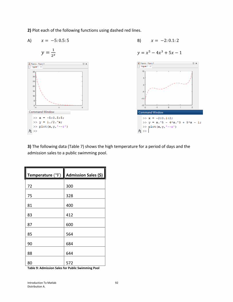
Introduction To Matlab 92 Distribution A.
2) Plot each of the following functions using dashed red lines.
A) 𝑥 = −5: 0.5: 5 B) 𝑥 = −2: 0.1: 2
𝑦 =1
2𝑥 𝑦 = 𝑥5 − 4𝑥3 + 5𝑥 − 1
3) The following data (Table 7) shows the high temperature for a period of days and the
admission sales to a public swimming pool.
Temperature (℉) Admission Sales ($)
72 300
75 328
81 400
83 412
87 600
85 564
90 684
88 644
80 572 Table 9: Admission Sales for Public Swimming Pool

Introduction To Matlab 93 Distribution A.
A) Store the data in a matrix called swim.
B) Create a graph of the data with the following specifications:
- Temperature is the x-value
- Admission Sales is the y-value
- Data points are represented by blue circles
- The graph is titled Swimming Pool Revenue
- Both x- and y-axes are labeled with units
1.42. RESOURCES
1. Mathworks®/MATLAB® Official Support Page:
https://www.mathworks.com/help/matlab/
2. An Introduction to Solving Engineering Problems with MATLAB® e-book:
https://www.ck12.org/book/Engineering%3A-An-Introduction-to-Solving-Engineering-
Problems-with-Matlab/

Introduction To Matlab 94 Distribution A.
CONDITIONAL STATEMENTS IN MATLAB®
1.43. INTRODUCTION
In this lesson, students will begin to create logic within a MATLAB® script using conditional
statements. Students will learn about each of the following: conditional/if statements in
MATLAB®, syntax for a conditional statement, common relational and logical operators, else
and else…if statements, and creating scripts that utilize conditional statements.
1.44. MATERIALS
Each student will need:
PC/Mac with MATLAB® installed
Copy of Introduction to MATLAB® - Conditional Statements in MATLAB® guided notes
(these may be printed or shared digitally): https://padlet.com/abrumbaugh/introMatlab
The teacher will need:
PC/MAC with MATLAB® installed
Ceiling projector or way to display their computer screen for students to see
Copy of Introduction to MATLAB® - Conditional Statements in MATLAB® answer key
1.45. OVERVIEW OF PLAN
This lesson can be taught via direct instruction or student-paced learning through online videos
located at https://padlet.com/abrumbaugh/introMatlab.
1.45.1. LEARNING TARGET – MATLAB.18
Be able to describe how a conditional/if statement works in computer programming.
A conditional statement, also commonly referred to as an if statement, is a statement that
allows the computer to make a logical decision. A conditional statement works by presenting
the computer with a logical statement (a statement that is either true or false) as a condition. If
an input makes the condition true, then the computer will perform a specific task. If the input
makes the condition false, then the computer will not perform the task. A detailed flowchart for
a conditional/if statement is given in the guided notes to help students better understand this
logical structure.

Introduction To Matlab 95 Distribution A.
It is very important that students understand conceptually how a conditional statement works.
Not only will this knowledge help students in creating conditional statements, but it will also
help them troubleshoot issues that may arise in their programs by stepping through the logical
steps that the conditional statement takes.
1.45.2. LEARNING TARGET – MATLAB.19
Be able to explain the meaning of the major logical operators in computer programming.
Conditional statements require the use of logical operators when setting up the condition to be
checked. For instance, should we check to see when a variable grows larger than a specified
value or should we check to see when a variable is equivalent to a specified value? Each of
these questions requires the use of a different logical operator to check the condition.
There are many different logical and relational operators; however, students will only need to
know some of the more commonly used ones (e.g., inequality symbols, and, or). A table of the
common logical and relational operators is provided for students in the guided notes.
Not only will knowledge of these operators be important for working with conditional
statements but will be used extensively in the next two lessons about loops.
1.45.3. LEARNING TARGET – MATLAB.20
Be able to utilize conditional statements in MATLAB® scripts.
After this lesson, students should become familiar with setting up and using conditional
statements within their scripts. A conditional statement has a multiline syntax that is a bit
different from what students have done up to this point.
To start a conditional statement, the keyword if must be typed followed by a logical statement
(i.e., the condition) that is to be checked by the computer. The next part of the conditional
statement is typed under the logical statement by pressing the Enter key. Here, students will
type the commands they wish the computer to run if an input value makes the condition true.
Lastly, the conditional statement must end with the keyword end to tell the computer that the
conditional statement is done. The general syntax for a conditional statement is shown in the
guided notes.
One thing to note when creating conditional statements in MATLAB® is the indentation that
MATLAB® uses. The list of commands within an if statement is indented 4 spaces to the right of
where the if statement started. While this indentation is not necessary for the program to run
correctly, there are many programming languages where the indentation is crucial. Therefore, it

Introduction To Matlab 96 Distribution A.
is considered best practice that any commands within an if statement or loop body are
indented 4 spaces from where the start of the if statement or loop begin.
1.46. GUIDED NOTES
Introduction to MATLAB
Conditional Statements in MATLAB
Name:___________________________ Date:_____________ Period:__________
Learning Targets:
MATLAB.18 – Be able to describe how a conditional/if statement works in computer
programming.
MATLAB.19 – Be able to explain the meaning of the major logical operators in computer
programming.
MATLAB.20 – Be able to utilize conditional statements in MATLAB scripts.
How Do Computers Make Decisions? (MATLAB.18)
There are times when we want a MATLAB script to perform different tasks depending on what
the user types. To accomplish this, we can use a conditional statement.
A conditional statement is a statement of the form _________________________ and allows
the computer to run a specific set of code in response to user input. The flowchart below
(Figure 11) illustrates the steps taken within a conditional/if statement.

Introduction To Matlab 97 Distribution A.
Logic of a Conditional Statement (MATLAB.18)
NO
Input
Condition:
Does the input make the
condition true?
YES
Run code under IF BLOCK
Continuation of
Program
Figure 11: Conditional Statement Flowchart. Created by author.

Introduction To Matlab 98 Distribution A.
Conditional Statements in MATLAB (MATLAB.18)
The syntax for a conditional statement in MATLAB is the following:
1) if <condition> 1) The <condition> will be a ________________________ that is
either TRUE or FALSE.
2) statement(s) 2) The statements are the commands the MATLAB will run
if the condition is _________.
3) end 3) Every if block must end with the keyword end.
NOTE: Make sure to use proper spacing. Statements after the if statement should be indented 4
spaces and the end keyword should align itself with the if statement.
Relational and Logical Operators in MATLAB (MATLAB.19)
The following symbols (Table 10) can be used to create a logical expression in a conditional
statement.
Symbol Meaning
<
<=
>
>=
==
~=
&& (AND)
|| (OR)
Table 10: Relational and Logical Operators

Introduction To Matlab 99 Distribution A.
Example 1 (MATLAB.18, 19)
Determine what will happen in each of the following scripts. In these examples if a condition is
NOT true, nothing will happen.
A)
B)
C)

Introduction To Matlab 100 Distribution A.
If…Else and Elseif Statements in MATLAB (MATLAB.18)
We can make conditional statements more versatile by using else or elseif blocks.
The else block of an if…else statement (Figure 12) is a section of code that runs when the
condition is ____________.
An elseif block (Figure ) in an if…else statement allows the script to check multiple
_________________ and execute the first of which is true.
Logic of an If…Else Statement (MATLAB.18)
NO
Input
Condition:
Does the input make the
condition true?
YES
Run code under ELSE
BLOCK
Continuation
of Program
Run code under IF
BLOCK
Figure 12: If...Else Statement. Created by author.

Introduction To Matlab 101 Distribution A.
Logic of an If…Elseif…Else Statement (MATLAB.18)
Example 2 (MATLAB.18, 19)
Determine the output will be for each of the following scripts.
A) B)
TRUE TRUE TRUE
Continuation of
Program
FALSE
Condition 3
Input
Condition 1
Condition 2
FALSE
FALSE
Perform action/code under
ELSE BLOCK
Run code under IF
BLOCK
Run code under ELSEIF
BLOCK 1 Run code under ELSEIF
BLOCK 2
Figure 13: If...Elseif...Else Statement. Created by author.

Introduction To Matlab 102 Distribution A.
Example 3 (MATLAB.18, 19)
Examine the script shown below.
For A – C, determine the output of the script for each of the following inputs:
A) numHours = 3
B) numHours = 15
C) numHours = 40
D) What number would the user have to type into the script to get the message, “How can you
play that many hours?”

Introduction To Matlab 103 Distribution A.
Example 4 (MATLAB.20)
A) Create a script that allows the user to type in two numbers. The script should then compare
the two numbers and state the relation between them (“a is larger than b”, “a is equal to b”,
etc.)
B) Create a script that will display the statement, “MATLAB is fun!” when the user types a
number that is less than or equal to 5 or greater than 11.
1.47. ASSESSMENT – PRACTICE PROBLEMS
Students should be able to complete the practice problems below to demonstrate their
understanding. Encourage students to refer to their notes, research online, or work together to
overcome any issues they may encounter. It is recommended that students receive a digital
version of these problems so that they can copy and paste their answers straight from
MATLAB®.
Practice Problems
1) A store that specializes in flooring offers special rates on carpet when purchased in certain
quantities. The table below shows the price for carpet and installation:
Amount (Square Feet) Price (Per Square Foot) Installation Fee (Per Square Foot)
1 – 100 $2.79 $1.75
101 – 200 $2.50 $1.50
201 – 400 $2.19 $1.25
401 – 800 $1.79 $1.00
More than 800 $1.50 Free

Introduction To Matlab 104 Distribution A.
Create a script that calculates the total cost (including 7.5% for tax) on any amount of carpet
that the user types in. The script should print the final amount in a well-formatted sentence.
The script should also let the user know if they typed in an invalid amount of carpet.
2) Suppose you are a design engineer for a company that manufactures consumer electronic
devices and you are estimating the cost of producing a new product. The product has four
components that are purchased from electronic parts suppliers and assembled in your factory.
You have received cost information from your suppliers for each of the parts; as is typical in the
electronics industry, the cost of a part depends on the number of parts you order from the
supplier.
Your assembly cost for each unit includes the cost of labor and your assembly plant. You have estimated that these costs are C0=$45.00/unit.
The cost of each part depends on the number of parts purchased; we will use the variable n to represent the number of parts, and the variables CA, CB, CC, and CD to represent the unit cost of each type of part. These costs are given in the table below.
Unit Cost of Part A
Unit Cost of Part B
Unit Cost of Part C
Unit Cost of Part D
Number of Parts (n)
CA Number of Parts (n)
CB Number of Parts (n)
CC Number of Parts (n)
CD
1 – 4 $16.00 1 – 9 $24.64 1 – 24 $17.98 1 – 9 $12.50
5 – 24 $14.00 10 – 49 $24.32 25 – 49 $16.78 10 – 99 $10.42
25 – 99 $12.70 50 – 99 $24.07 50 or more $15.78 100 or more $9.62
100 or more
$11.00 100 or more
$23.33

Introduction To Matlab 105 Distribution A.
The unit cost is unit = C0 + CA + CB + CC + CD.
To find the unit cost to build one unit, we look in the above tables with a value of n = 1; the unit cost is $45.00+ $16.00+ $24.64+ $17.98+ $12.50= $116.12 To find the unit cost to build 20 units, we look in the above tables with a value of n = 20 and get $45.00+ $14.00+ $24.32+ $17.98+ $10.42= $109.72 As expected, the unit cost for 20 units is lower than the unit cost for one unit.
Create a script that asks for the total number of parts needed, n, and computes the total unit
cost for the new product. (Morrell & Gjendemsjø, 2012)
Morrell, Darryl, and Anders Gjendemsjø. "An Introduction to Solving Engineering Problems with MATLAB." CK-12, CK-12, 23
Feb. 2012, www.ck12.org/book/Engineering%3A-An-Introduction-to-Solving-Engineering-Problems-with-Matlab/. Accessed 26
June 2018.
1.48. ANSWER KEYS
1.48.1. GUIDED NOTES
Introduction to MATLAB
Conditional Statements in MATLAB
Name:___________________________ Date:_____________ Period:__________
Learning Targets:
MATLAB.18 – Be able to describe how a conditional/if statement works in computer
programming.

Introduction To Matlab 106 Distribution A.
MATLAB.19 – Be able to explain the meaning of the major logical operators in computer
programming.
MATLAB.20 – Be able to utilize conditional statements in MATLAB scripts.
How Do Computers Make Decisions? (MATLAB.18)
There are times when we want a MATLAB script to perform different tasks depending on what
the user types. To accomplish this, we can use a conditional statement.
A conditional statement is a statement of the form if…then… and allows the computer to run a
specific set of code in response to user input. The flowchart below (Figure 11) illustrates the
steps taken within a conditional/if statement.
Logic of a Conditional Statement (MATLAB.18)
NO
Input
Condition:
Does the input make the
condition true?
YES
Run code under IF BLOCK
Continuation of
Program
Figure 14: Conditional Statement Flowchart. Created by author.

Introduction To Matlab 107 Distribution A.
Conditional Statements in MATLAB (MATLAB.18)
The syntax for a conditional statement in MATLAB is the following:
1) if <condition> 1) The <condition> will be a logical/Boolean expression that is
either TRUE or FALSE.
2) statement(s) 2) The statements are the commands the MATLAB will run
if the condition is TRUE.
3) end 3) Every if block must end with the keyword end.
NOTE: Make sure to use proper spacing. Statements after the if statement should be indented 4
spaces and the end keyword should align itself with the if statement.
Relational and Logical Operators in MATLAB (MATLAB.19)
The following symbols (Table 10) can be used to create a logical expression in a conditional
statement.
Symbol Meaning
< Less than
<= Less than or equal to
> Greater than
>= Greater than or equal to
== Equal to/Same
~= Not equal to
&& (AND) Used to join two or more conditions. Evaluates to TRUE when ALL conditions are true.
|| (OR) Used to join two or more conditions. Evaluates to TRUE when at least one condition is true.
Table 10: Relational and Logical Operators

Introduction To Matlab 108 Distribution A.
Example 1 (MATLAB.18, 19)
Determine what will happen in each of the following scripts. In these examples if a condition is
NOT true, nothing will happen.
A)
The script will display “a is less than 5”
B)
The script will calculate 2.5 * 4 since 2.5 > 0, and store the answer in x.
The script will then display “10”.
C)
The script will not do anything since the condition (c < 0) is not true.
If…Else and Elseif Statements in MATLAB (MATLAB.18)
We can make conditional statements more versatile by using else or elseif blocks.
The else block of an if…else statement (Figure 12) is a section of code that runs when the
condition is FALSE.

Introduction To Matlab 109 Distribution A.
An elseif block (Figure 13) in an if…else statement allows the script to check multiple conditions
and execute the first of which is true.
Logic of an If…Else Statement (MATLAB.18)
NO
Input
Condition:
Does the input make the
condition true?
YES
Run code under ELSE
BLOCK
Continuation
of Program
Run code under IF
BLOCK
Figure 17: If...Else Statement. Created by author.

Introduction To Matlab 110 Distribution A.
Logic of an If…Elseif…Else Statement (MATLAB.18)
Example 2 (MATLAB.18, 19)
Determine the output for each of the following scripts.
A)
TRUE TRUE TRUE
Continuation of
Program
FALSE
Condition 3
Input
Condition 1
Condition 2
FALSE
FALSE
Perform action/code under
ELSE BLOCK
Run code under IF
BLOCK
Run code under ELSEIF
BLOCK 1 Run code under ELSEIF
BLOCK 2
Figure 18: If...Elseif...Else Statement. Created by author.

Introduction To Matlab 111 Distribution A.
Since myGrade >= 60 is TRUE when myGrade = 67, the output will be, “You are passing the
class.”
B)
The second condition (item >= 10 && item < 15) is the true condition when item = 10.
Therefore, the script will perform the calculation: cost = 2.75 * 10 + 5. The answer 32.50 will be
displayed on the screen.
Example 3 (MATLAB.18, 19)
Examine the script shown below.
For A – C, determine the output of the script for each of the following inputs:
A) numHours = 3
An input of 3 makes the second condition true. The message, “You must be busy with other
things.” will be displayed.

Introduction To Matlab 112 Distribution A.
B) numHours = 15
An input of 15 makes the fourth condition true. The message, “You must have a lot of free
time.” will be displayed.
C) numHours = 40
An input of 40 makes the fourth condition true. The message, “You must have a lot of free
time.” will be displayed.
D) What number would the user have to type into the script to get the message, “How can you
play that many hours?”
For this to occur, the first four conditions must be false. The first condition covers an input of 0;
the second condition covers input values larger than 0 but less than or equal to 5; the third
condition covers input values larger than 5 but less than or equal to 10; and the fourth
condition covers all input values larger than 10. The only input values not addressed by the
conditions are the numbers that are less than 0 (i.e., negative numbers.) Any negative input
value will cause all four conditions to fail and the message, “How can you play that many
hours?” to be displayed.
Example 4 (MATLAB.20)
A) Create a script that allows the user to type in two numbers. The script should then compare
the two numbers and state the relation between them (“a is larger than b”, “a is equal to b”,
etc.)
B) Create a script that will display the statement, “MATLAB is fun!” when the user types a
number that is less than or equal to 5 or greater than 11.
NOTE: There are many ways to create this script. This is one way.

Introduction To Matlab 113 Distribution A.
1.48.2. PRACTICE PROBLEMS
Practice Problems
NOTE: There are multiple ways to create the scripts in these problems. One example solution is
provided.
1) A store that specializes in flooring offers special rates on carpet when purchased in certain
quantities. The table below shows the price for carpet and installation:
Create a script that calculates the total cost (including 7.5% for tax) on any amount of carpet
that the user types in. The script should print the final amount in a well-formatted sentence.
The script should also let the user know if they typed in an invalid amount of carpet.
Amount (Square Feet) Price (Per Square Foot) Installation Fee (Per Square Foot)
1 – 100 $2.79 $1.75
101 – 200 $2.50 $1.50
201 – 400 $2.19 $1.25
401 – 800 $1.79 $1.00
More than 800 $1.50 Free
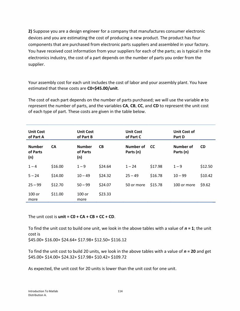
Introduction To Matlab 114 Distribution A.
2) Suppose you are a design engineer for a company that manufactures consumer electronic
devices and you are estimating the cost of producing a new product. The product has four
components that are purchased from electronic parts suppliers and assembled in your factory.
You have received cost information from your suppliers for each of the parts; as is typical in the
electronics industry, the cost of a part depends on the number of parts you order from the
supplier.
Your assembly cost for each unit includes the cost of labor and your assembly plant. You have estimated that these costs are C0=$45.00/unit.
The cost of each part depends on the number of parts purchased; we will use the variable n to represent the number of parts, and the variables CA, CB, CC, and CD to represent the unit cost of each type of part. These costs are given in the table below.
Unit Cost of Part A
Unit Cost of Part B
Unit Cost of Part C
Unit Cost of Part D
Number of Parts (n)
CA Number of Parts (n)
CB Number of Parts (n)
CC Number of Parts (n)
CD
1 – 4 $16.00 1 – 9 $24.64 1 – 24 $17.98 1 – 9 $12.50
5 – 24 $14.00 10 – 49 $24.32 25 – 49 $16.78 10 – 99 $10.42
25 – 99 $12.70 50 – 99 $24.07 50 or more $15.78 100 or more $9.62
100 or more
$11.00 100 or more
$23.33
The unit cost is unit = C0 + CA + CB + CC + CD.
To find the unit cost to build one unit, we look in the above tables with a value of n = 1; the unit cost is $45.00+ $16.00+ $24.64+ $17.98+ $12.50= $116.12 To find the unit cost to build 20 units, we look in the above tables with a value of n = 20 and get $45.00+ $14.00+ $24.32+ $17.98+ $10.42= $109.72 As expected, the unit cost for 20 units is lower than the unit cost for one unit.
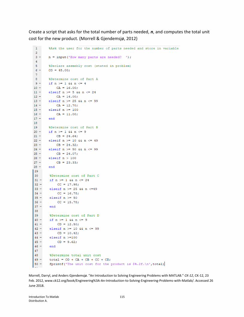
Introduction To Matlab 115 Distribution A.
Create a script that asks for the total number of parts needed, n, and computes the total unit
cost for the new product. (Morrell & Gjendemsjø, 2012)
Morrell, Darryl, and Anders Gjendemsjø. "An Introduction to Solving Engineering Problems with MATLAB." CK-12, CK-12, 23
Feb. 2012, www.ck12.org/book/Engineering%3A-An-Introduction-to-Solving-Engineering-Problems-with-Matlab/. Accessed 26
June 2018.

Introduction To Matlab 116 Distribution A.
1.49. RESOURCES
1. Mathworks®/MATLAB® Official Support Page:
https://www.mathworks.com/help/matlab/
2. An Introduction to Solving Engineering Problems with MATLAB® e-book:
https://www.ck12.org/book/Engineering%3A-An-Introduction-to-Solving-Engineering-
Problems-with-Matlab/

Introduction To Matlab 117 Distribution A.
INTRODUCTION TO LOOPS: FOR LOOPS
1.50. INTRODUCTION
In this lesson, students will be introduced to looping. Students will learn about the structure of
for loops, how to step through and explain each step of a for loop, as well as how to create for
loops to perform small programming tasks and graphing.
1.51. MATERIALS
Each student will need:
PC/Mac with MATLAB® installed
Copy of Introduction to MATLAB® - Introduction to Loops: For Loops guided notes (these
may be printed or shared digitally): https://padlet.com/abrumbaugh/introMatlab
The teacher will need:
PC/MAC with MATLAB® installed
Ceiling projector or way to display their computer screen for students to see
Copy of Introduction to MATLAB® - Introduction to Loops: For Loops answer key
1.52. OVERVIEW OF PLAN
This lesson can be taught via direct instruction or student-paced learning through online videos
located at https://padlet.com/abrumbaugh/introMatlab.
1.52.1. LEARNING TARGET – MATLAB.21
Be able to explain how a for loop works in MATLAB® and other programming languages.
For loops are a common structure found in MATLAB® and other programming languages. The
logic behind a for loop is important for students to understand as they are used heavily in
MATLAB® and many other programming languages.
A for loop is a structure within a program that repeats a section of code multiple times. The
number of iterations (i.e., repetitions) is based on the end value of an index variable (i.e.,
counter). After each execution of the code, the index variable increases by 1 until it has reached
its end value. Once the end value is reached, the loop terminates and any code occurring after
the loop will be executed.

Introduction To Matlab 118 Distribution A.
Students should be able to analyze a for loop and explain what value(s) it will output. Students
should also be able to explain what the loop does at various points during its execution.
1.52.2. LEARNING TARGET – MATLAB.22
Be able to utilize for loops in MATLAB® scripts.
After this lesson, students should be able to create for loops for a variety of situations from
evaluating a mathematical function, creating a graph, and performing a series of calculations to
solve a problem. It is important to note that for loops can be used in many situations, and that
this lesson covers a very limited number of those situations.
Loops can be difficult for students, especially students with little to no programming
background. This lesson may take a few days for students to complete. As students begin to
create their own for loops, encourage them to step through the code line by line either
mentally or, preferably, on paper. This will not only help with troubleshooting should problems
arise in their code but will also help students process the logical steps that occur during a for
loop.
1.53. GUIDED NOTES
Introduction to MATLAB
Introduction to Loops: For Loops
Name:___________________________ Date:_____________ Period:__________
Learning Targets:
MATLAB.21 – Be able to explain how a for loop works in MATLAB and other programming
languages.
MATLAB.22 – Be able to utilize for loops in MATLAB scripts.
What is a Loop? (MATLAB.21)
There may be situations where we want parts of a program to be used multiple times (e.g.,
performing a series of calculations on a list of numbers, run a program multiple times based on
user input). To achieve this functionality, we can use what is commonly referred to as a loop in
computer programming.
Loops are structures that allow code to be ___________________ until certain conditions are
met.

Introduction To Matlab 119 Distribution A.
One type of loop that can be used is a for loop (Figure and Figure ). A for loop will repeat code
_________________________________________________________________________
Logic of a For Loop (MATLAB.21)
For Loops in MATLAB (MATLAB.21)
The syntax for a for loop in MATLAB is as follows:
1) for index/counter = array/values 1) The index/counter is a ___________ that stores
the values to be iterated through the loop. Line
must begin with the keyword ________.
Start
Define Array:
(x = start:increment:end)
Check Condition:
Are there anymore
elements in the array?
Run code in loop body for
the selected element
True
Increment Index:
(Move to next element of Array)
False
End
Figure 22: For Loop in MATLAB® Created by author.
Initialize Index/Counter:
(x = 0)
Check Condition:
Is counter’s value less
than a given value?
Run code in loop body
True
Increment Counter
(x = x + 1)
False
Start
End
Figure 23: Traditional For Loop. Created by author.

Introduction To Matlab 120 Distribution A.
2) statement(s) 2) The statements are the commands that MATLAB
will run using the values stored in the
___________________.
3) end 3) Every for loop block must end with the keyword
__________.
Example of For Loop in MATLAB (MATLAB.21)
In this example, i represents the ___________________ of the for loop, and its values range
from ______________.
Beginning with i = 1, the statements in the loop body are executed:
d = i + 12
disp(d)
Once the body is completed, the program returns to the first line and changes the value of i to
__________________________________________________, or i = ________. The process
continues in this manner until all values specified by the index/counter have been used.
Here is what the example would look like as a flowchart (Figure 15):
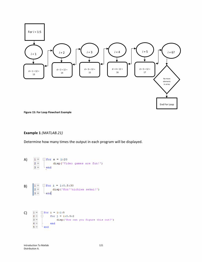
Introduction To Matlab 121 Distribution A.
Example 1 (MATLAB.21)
Determine how many times the output in each program will be displayed.
A)
B)
C)
i = 2
d = 2 + 12 =
14
i = 3
d = 3 + 12 =
15
i = 4
d = 4 + 12 =
16
i = 1
d = 1 + 12 =
13
For i = 1:5
No more
elements
in array
End For Loop
i = 5
d = 5 + 12 =
17
i = 6?
Figure 15: For Loop Flowchart Example

Introduction To Matlab 122 Distribution A.
Example 2 (MATLAB.21)
What sequence of numbers will the following loop print? Explain why this code does what it
does.
Example 3 (MATLAB.21)
A) What value will be displayed when this script is ran?
B) How could we find this answer more quickly using math?
Example 4 (MATLAB.22)
A) Create a for loop that will take the values from -5 to 5 and multiply them by 3.

Introduction To Matlab 123 Distribution A.
a
b
c
B) Create a for loop that will evaluate the function 𝑦 = 2𝑥2 − 3𝑥 + 1 for all values of x from 1
and 10.
C) Use a for loop to graph 𝑦 = cos (2𝜋𝑓𝑡) for values of t from 0 to 4 and for the following values
of f: 0.5, 1, 1.8, and 2.6.
Example 5 (MATLAB.22)
Suppose you are modifying an RC car and are designing wheels that will achieve a given travel
speed. The radius (in inches) of the wheel is represented by r, and the rotations per second by
the wheel is represented by w. The speed of the car (s) in inches per second can be found by
using the formula 𝑠 = 2𝜋𝑟𝑤.
On a single graph, create plots of the relationship between s and w for the following r values:
0.4 in., 0.7 in., 1.3 in., 3.2 in., and 4.0 in.
Example 6 (MATLAB.22)
The following table represents different lengths of the legs of a right triangle.
Use a for loop and the Pythagorean Theorem to determine the length of the hypotenuse (c) for
each pair of leg values.
a b
1 1
2 3
4 2
7 3
a
b
c
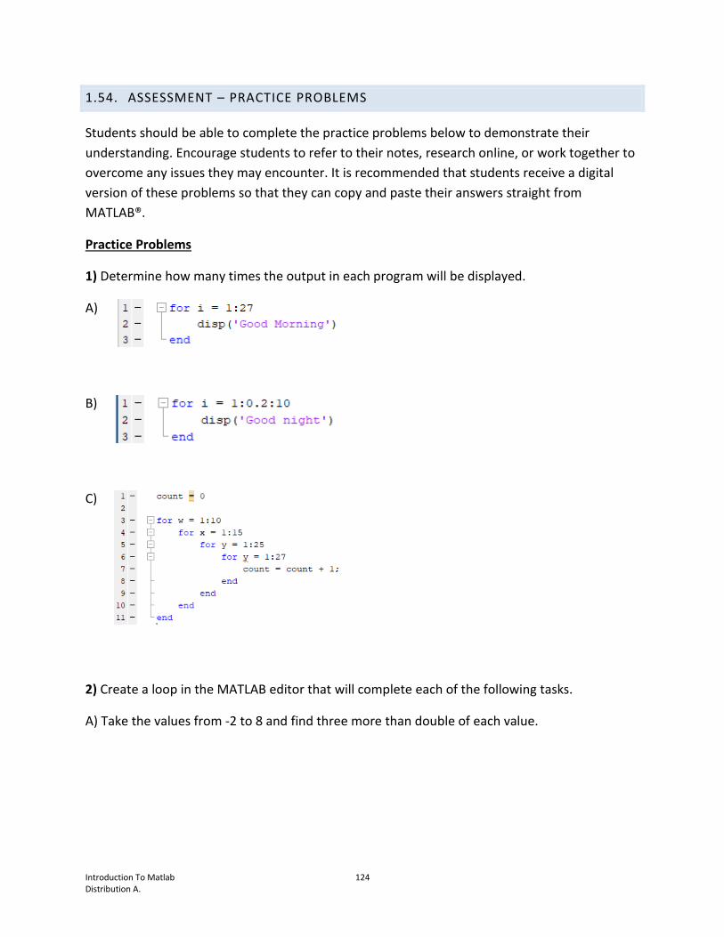
Introduction To Matlab 124 Distribution A.
1.54. ASSESSMENT – PRACTICE PROBLEMS
Students should be able to complete the practice problems below to demonstrate their
understanding. Encourage students to refer to their notes, research online, or work together to
overcome any issues they may encounter. It is recommended that students receive a digital
version of these problems so that they can copy and paste their answers straight from
MATLAB®.
Practice Problems
1) Determine how many times the output in each program will be displayed.
A)
B)
C)
2) Create a loop in the MATLAB editor that will complete each of the following tasks.
A) Take the values from -2 to 8 and find three more than double of each value.

Introduction To Matlab 125 Distribution A.
B) Plot the graph of ℎ = −4.9𝑡2 + 45𝑡 + 3 for the t-values of 0, 1.7, 2.9, and 4.
3) Use the distance formula, 𝑑 = √(𝑥2 − 𝑥1)2 + (𝑦2 − 𝑦1)2 , to determine the distance
between each set of consecutive points in the table.
4) Suppose a cylinder has a height h and base diameter of b, and you want to find out how
many ping-pong balls of diameter d could fit into the cylinder. To figure this out, we need to
learn how to compute the lower bound on the number of ping-pong balls.
A lower bound for this problem can be found using the following:
𝑁𝐿 – Lower bound on the number of balls that fit into the cylinder. 𝑁𝐿 =𝑉𝑐𝑦𝑙
𝑉𝑐𝑢𝑏𝑒
𝑉𝑐𝑦𝑙 – The volume of the cylinder. 𝑉𝑐𝑦𝑙 = 𝜋 (𝑏
2)2
ℎ
𝑉𝑐𝑢𝑏𝑒 – The volume of a cube that encloses a single ball. 𝑉𝑐𝑢𝑏𝑒 = 𝑑3
x y
1 1
2 -4
3 8
4 5
5 -1
6 3

Introduction To Matlab 126 Distribution A.
A) Use the command line prompt to determine the lower bound of the ping-pong balls given
that d = 1.54 in., b = 8 in., and h = 14 in.
B) Create a script that would allow you to solve the problem in A).
C) Add a for loop to your script to compute 𝑁𝐿 for b = 8 in. and h = 14 in. Let the values of d
range from 1 in. to 2 in., incrementing each value by 0.1 in.
D) Add a plot function to your script to plot 𝑁𝐿 as a function of d for b = 8 in. and h = 14 in.
E) Modify your script to compute 𝑁𝐿 for d = 1.54 in. and various values of b and h (at least 10
values for each)
1.55. ANSWER KEYS
1.55.1. GUIDED NOTES
Introduction to MATLAB
Introduction to Loops: For Loops
Name:___________________________ Date:_____________ Period:__________
Learning Targets:
MATLAB.21 – Be able to explain how a for loop works in MATLAB and other programming
languages.
MATLAB.22 – Be able to utilize for loops in MATLAB scripts.
What is a Loop? (MATLAB.21)
There may be situations where we want parts of a program to be used multiple times (e.g.,
performing a series of calculations on a list of numbers, run a program multiple times based on

Introduction To Matlab 127 Distribution A.
user input). To achieve this functionality, we can use what is commonly referred to as a loop in
computer programming.
Loops are structures that allow code to be repeated until certain conditions are met.
One type of loop that can be used is a for loop (Figure and Figure ). A for loop will repeat code a
specific number of times based on a value of the index variable/counter.
Logic of a For Loop (MATLAB.21)
For Loops in MATLAB (MATLAB.21)
The syntax for a for loop in MATLAB is as follows:
Start
Define Array:
(x = start:increment:end)
Check Condition:
Are there anymore
elements in the array?
Run code in loop body for
the selected element
True
Increment Index:
(Move to next element of Array)
False
End
Figure 22: For Loop in MATLAB®
Initialize Index/Counter:
(x = 0)
Check Condition:
Is counter’s value less
than a given value?
Run code in loop body
True
Increment Counter
(x = x + 1)
False
Start
End
Figure 23: Traditional For Loop

Introduction To Matlab 128 Distribution A.
1) for index/counter = array/values 1) The index/counter is a variable that stores
the values to be iterated through the loop. Line
must begin with the keyword for.
2) statement(s) 2) The statements are the commands that MATLAB
will run using the values stored in the
index/counter.
3) end 3) Every for loop block must end with the keyword
end.
Example of For Loop in MATLAB (MATLAB.21)
In this example, i represents the index/counter of the for loop, and its values range from 1 to 5.
Beginning with i = 1, the statements in the loop body are executed:
d = i + 12 d = 1 + 12 = 13
disp(d) 13
Once the body is completed, the program returns to the first line and changes the value of i to
the next value of the index/counter, or i = 2. The process continues in this manner until all
values specified by the index/counter have been used.
Here is what the example would look like as a flowchart (Figure 15):

Introduction To Matlab 129 Distribution A.
Example 1 (MATLAB.21)
Determine how many times the output in each program will be displayed.
A)
‘Video games are fun!’ will be displayed 20 times.
B)
‘Kon’nichiwa sekai!’ will be displayed 59 times.
C)
‘How can you figure this out?’ will be displayed 15 times.
Example 2 (MATLAB.21)
i = 2
d = 2 + 12 =
14
i = 3
d = 3 + 12 =
15
i = 4
d = 4 + 12 =
16
i = 1
d = 1 + 12 =
13
For i = 1:5
No more
elements
in array
End For Loop
i = 5
d = 5 + 12 =
17
i = 6?
Figure 24: For Loop Flowchart Example. Created by author.

Introduction To Matlab 130 Distribution A.
What sequence of numbers will the following loop print? Explain why this code does what it
does.
Sequence: 6, 5, 4, 3, 2, 1, 0
In this code, a starts with a value of 7. The loop counter will execute from 1 to 7, for a total of 7
times. Each time the loop body executes, it takes the current value of a and subtracts 1 from it.
This new value is re-stored in a and is displayed on the screen.
When 7 is passed through the loop for the first time, its value becomes 6 (i.e., a = 7 – 1), and is
displayed before the loop body executes again. The table below (Table 8) shows how the
variable values change throughout the loop.
j (index/counter) a a = a – 1 disp(a)
1 7 7 – 1 6
2 6 6 – 1 5
3 5 5 – 1 4
4 4 4 – 1 3
5 3 3 – 1 2
6 2 2 – 1 1
7 1 1 – 1 0 Table 8: Example 2 Loop Analysis
Example 3 (MATLAB.21)

Introduction To Matlab 131 Distribution A.
A) What value will be displayed when this script is ran?
3000
B) How could we find this answer more quickly using math?
Determine the number of times each loop will activate and multiply the values together (i.e., a
will loop 5 times, b will loop 10 times, c will loop 20 times, and d will loop 3 times):
5 ∗ 10 ∗ 20 ∗ 3 = 3000
Example 4 (MATLAB.22)
A) Create a for loop that will take the values from -5 to 5 and multiply them by 3.
B) Create a for loop that will evaluate the function 𝑦 = 2𝑥2 − 3𝑥 + 1 for all values of x from 1
and 10.
C) Use a for loop to graph 𝑦 = cos (2𝜋𝑓𝑡) for values of t from 0 to 4 and for the following values
of f: 0.5, 1, 1.8, and 2.6.

Introduction To Matlab 132 Distribution A.
a
b
c
Example 5 (MATLAB.22)
Suppose you are modifying an RC car and are designing wheels that will achieve a given travel
speed. The radius (in inches) of the wheel is represented by r, and the rotations per second by
the wheel is represented by w. The speed of the car (s) in inches per second can be found by
using the formula 𝑠 = 2𝜋𝑟𝑤.
On a single graph, create plots of the relationship between s and w for the following r values:
0.4 in., 0.7 in., 1.3 in., 3.2 in., and 4.0 in.
Example 6 (MATLAB.22)
The following table represents different lengths of the legs of a right triangle.
Use a for loop and the Pythagorean Theorem to determine the length of the hypotenuse (c) for
each pair of leg values.
a b
1 1
2 3
4 2
7 3
a
b
c
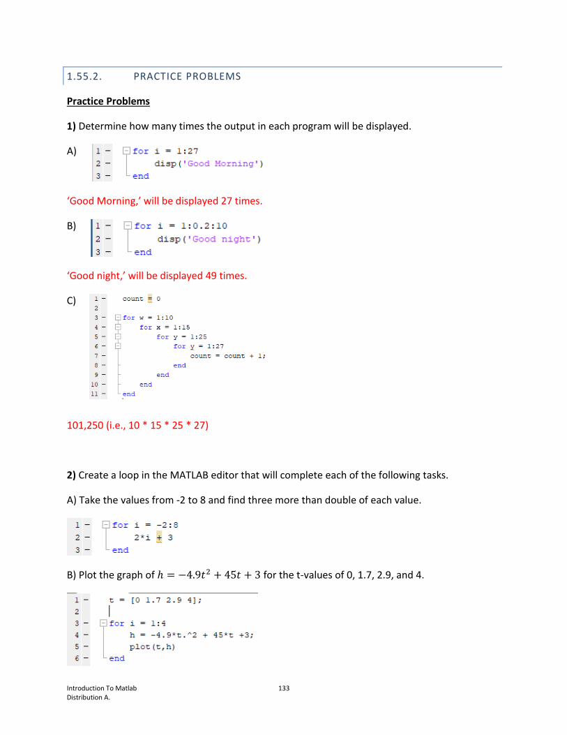
Introduction To Matlab 133 Distribution A.
1.55.2. PRACTICE PROBLEMS
Practice Problems
1) Determine how many times the output in each program will be displayed.
A)
‘Good Morning,’ will be displayed 27 times.
B)
‘Good night,’ will be displayed 49 times.
C)
101,250 (i.e., 10 * 15 * 25 * 27)
2) Create a loop in the MATLAB editor that will complete each of the following tasks.
A) Take the values from -2 to 8 and find three more than double of each value.
B) Plot the graph of ℎ = −4.9𝑡2 + 45𝑡 + 3 for the t-values of 0, 1.7, 2.9, and 4.

Introduction To Matlab 134 Distribution A.
3) Use the distance formula, 𝑑 = √(𝑥2 − 𝑥1)2 + (𝑦2 − 𝑦1)
2 , to determine the distance
between each set of consecutive points in the table.
4) Suppose a cylinder has a height h and base diameter of b, and you want to find out how
many ping-pong balls of diameter d could fit into the cylinder. To figure this out, we need to
learn how to compute the lower bound on the number of ping-pong balls.
A lower bound for this problem can be found using the following:
𝑁𝐿 – Lower bound on the number of balls that fit into the cylinder. 𝑁𝐿 =𝑉𝑐𝑦𝑙
𝑉𝑐𝑢𝑏𝑒
𝑉𝑐𝑦𝑙 – The volume of the cylinder. 𝑉𝑐𝑦𝑙 = 𝜋 (𝑏
2)2
ℎ
𝑉𝑐𝑢𝑏𝑒 – The volume of a cube that encloses a single ball. 𝑉𝑐𝑢𝑏𝑒 = 𝑑3
A) Use the command line prompt to determine the lower bound of the ping-pong balls given
that d = 1.54 in., b = 8 in., and h = 14 in.
x y
1 1
2 -4
3 8
4 5
5 -1
6 3

Introduction To Matlab 135 Distribution A.
B) Create a script that would allow you to solve the problem in A).
C) Add a for loop to your script to compute 𝑁𝐿 for b = 8 in. and h = 14 in. Let the values of d
range from 1 in. to 2 in., incrementing each value by 0.1 in.
D) Add a plot function to your script to plot 𝑁𝐿 as a function of d for b = 8 in. and h = 14 in.

Introduction To Matlab 136 Distribution A.
E) Modify your script to compute 𝑁𝐿 for d = 1.54 in. and various values of b and h (at least 10
values for each).
1.56. RESOURCES
1. Mathworks®/MATLAB® Official Support Page:
https://www.mathworks.com/help/matlab/
2. An Introduction to Solving Engineering Problems with MATLAB® e-book:
https://www.ck12.org/book/Engineering%3A-An-Introduction-to-Solving-Engineering-
Problems-with-Matlab/

Introduction To Matlab 137 Distribution A.
INTRODUCTION TO LOOPS: WHILE LOOPS
1.57. INTRODUCTION
In this lesson, students will continue their work with loops, advancing on to while loops.
Students will learn about the structure of while loops, how to step through and explain each
line of code in a while loop, as well as how to create while loops to perform small programming
tasks.
1.58. MATERIALS
Each student will need:
PC/Mac with MATLAB® installed
Copy of Introduction to MATLAB® - Introduction to Loops: While Loops guided notes
(these may be printed or shared digitally): https://padlet.com/abrumbaugh/introMatlab
The teacher will need:
PC/MAC with MATLAB® installed
Ceiling projector or way to display their computer screen for students to see
Copy of Introduction to Loops: While Loops answer key
1.59. OVERVIEW OF PLAN
This lesson can be taught via direct instruction or student-paced learning through online videos
located at https://padlet.com/abrumbaugh/introMatlab.
1.59.1. LEARNING TARGET – MATLAB.23
Be able to explain how a while loop works in MATLAB® and other programming languages.
Just like for loops from the previous lesson, while loops are structures that are used to repeat a
specific section of code. While loops are used quite extensively in MATLAB® as well as other
programming languages.
A for loop iterates over a section of code a specific number of times (i.e., the index variable has
a start and end value), whereas a while loop will continue to iterate until a specific condition is
met or fails. It is important that the students understand the logic that drives a while loop and
be able to explain what happens at various points when a while loop executes.

Introduction To Matlab 138 Distribution A.
1.59.2. LEARNING TARGET – MATLAB.24
Be able to utilize while loops in MATLAB® scripts.
After this lesson, students should be able to create while loops for a variety of situations
including divisibility tests and simple games. This lesson only covers a small sample of while
loop problems, but many more exist. In fact, many problems containing a for loop could be
reconfigured to use a while loop too.
Loops can be difficult for students, especially students with little to no programming
background. This lesson may take a few days for students to complete. As students begin to
create their own while loops, encourage them to step through the code line by line either
mentally or, preferably, on paper. This will not only help with troubleshooting should problems
arise in their code but will also help students process the logical steps that occur during a while
loop.
1.60. GUIDED NOTES
Introduction to MATLAB
Introduction to Loops: While Loops
Name:___________________________ Date:_____________ Period:__________
Learning Targets:
MATLAB.23 – Be able to explain how a while loop works in MATLAB and other programming
languages.
MATLAB.24 – Be able to utilize while loops in MATLAB scripts.
What is a While Loop? (MATLAB.23)
A while loop is a loop (Figure 16) that will execute a body of code until a specific
_______________________________ is met.

Introduction To Matlab 139 Distribution A.
Logic of a While Loop (MATLAB.23)
While Loops in MATLAB (MATLAB.23)
The syntax for a while loop in MATLAB is as follows:
1) while <expression> 1) The expression is a logical expression (i.e., it is
either true or false) that determines if the loop
body is executed. Line must begin with the
keyword _____________.
2) statement(s) 2) The statements are the commands that MATLAB will
run only when the logical expression from the while
statement is _____________.
Start
Check Condition:
A logical expression that
evaluates to true or false
Run code in loop body for the
selected element
True
Update Variable Values
False
End
Figure 16: While Loop in MATLAB®. Created by author.

Introduction To Matlab 140 Distribution A.
Figure 17: Sample While Loop
3) end 3) Every while loop block must end with the keyword
___________.
Example of While Loop in MATLAB (MATLAB.23)
In this example (Figure 17), the variables a, b, and total are ____________________, meaning
that they are given values prior to entering the loop. This must be done as the program will
NOT recognize them when it begins the loop otherwise.
Once the program reaches the while loop, it checks to see if the sum of a and b is
________________________ total. When this condition is true, the loop body is executed.
First run of while loop:
a = 3, b = 2, total = 40
Check Condition: a + b < 40? TRUE / FALSE
If true:
a = a * 2
b = b * 2
fprintf(…)

Introduction To Matlab 141 Distribution A.
Once the body is completed, the program returns to the while loop statement and checks to
see if ____________________________. The program will continue this process until this
condition is false.
Here is what the example would look like as a flowchart (Figure 18):
Example 1 (MATLAB.23)
Determine the number of times each string will be printed in each script.
A)
B)
a = 12
b = 8 a = 24
b = 16
a = 12 * 2 = 24
b = 8 * 2 = 16
FalTr
True
a = 3 * 2 = 6
b = 2 * 2 = 4
a = 3, b = 2
total = 40
(Initialize)
Condition:
a + b < total?
a = 6
b = 4
End While
Loop
Condition:
a + b < total?
a = 6 * 2 = 12
b = 4 * 2 = 8
Condition:
a + b < total? Condition:
a + b < total?
True True False
Figure 18: While Loop Flowchart Example. Created by author.

Introduction To Matlab 142 Distribution A.
Example 2 (MATLAB.23)
Determine the number of times the string will be printed in the following script.
Why does the script act the way that it does? Explain.
Example 3 (MATLAB.23)
What values will the following code print?
Example 4 (MATLAB.24)
Use a while loop to solve each of the following problems.
A) Create a script that asks the user to input a value that is greater than 0. The script should
keep asking until a valid number is entered.
B) Create a script that asks the user to enter two numbers and determines if the sum of the
numbers is even. An even number is one that is divisible by 2. The script should continue asking
for two numbers until their sum is even.

Introduction To Matlab 143 Distribution A.
NOTE: You will need to use the b = mod(a,m) mathematical function (mod is short for modular
arithmetic). Mod calculates the remainder of a / m.
Examples:
mod(10,2) = 0 mod(10,3) = 1 mod(8,3) = 2 mod(125,6) = 5
C) Create a number guess game where a random integer from 1 to 20 is chosen, and the player
gets a maximum of three chances to guess the correct number. After each guess, the player
should receive feedback that tells them whether their guess was too low or too high. The
program should congratulate the player if they guess the correct number within the guess limit;
and the program should tell the player what number it had chosen if three incorrect guesses
have been made.
NOTE: To generate a random integer, use the randi(imax) function of MATLAB. The function
works by replacing imax with a positive integer value. The program will then select a random
integer between 1 and the value imax is equal to.
Example: a = randi(10) The value of a will be number selected randomly from 1 to 10.
1.61. ASSESSMENT – PRACTICE PROBLEMS
Students should be able to complete the practice problems below to demonstrate their
understanding. Encourage students to refer to their notes, research online, or work together to
overcome any issues they may encounter. It is recommended that students receive a digital
version of these problems so that they can copy and paste their answers straight from
MATLAB®.
Practice Problems

Introduction To Matlab 144 Distribution A.
1) Determine the number of times each string will print in the following scripts.
A)
B)
C)
D)
2) Use a while loop to solve each of the following problems.
A) Create a script that displays the consecutive integers from 10 to 20.

Introduction To Matlab 145 Distribution A.
B) Create a script that asks the user to enter two numbers and determines if the difference of
the numbers is a multiple of 6 (e.g., 6, 12, 18, 24… are multiples of 6). The script should
continue asking for two numbers until their difference is a multiple of 6.
3) Create a game of rock-paper-scissors in MATLAB. Here are the requirements:
Utilize a while loop to determine when the game is over
Player should be able to choose rock, paper, or scissors on his/her turn
o NOTE: You may use numeric values to represent each item (e.g., “Press 1 for
rock,…”), but be sure to communicate this clearly to players through your
program
The computer will randomly pick rock, paper, or scissors for each round
The program should compare the choices made by the player and computer to see who
wins the round
o Rules: rock beats scissors, paper beats rock, scissors beat paper
One point is awarded to the player who wins a round
The game is over when either the player or computer earns three points
When the game is over, a message should display based on whether a player won or lost
o Example: “Congratulations!” or “Nice try!”
Your program will require the use of a while loop, conditional statements, input functions, and
other topics covered throughout the previous lessons. Good luck!
1.62. ANSWER KEYS
1.62.1. GUIDED NOTES
Introduction to MATLAB
Introduction to Loops: While Loops
Name:___________________________ Date:_____________ Period:__________
Learning Targets:

Introduction To Matlab 146 Distribution A.
MATLAB.23 – Be able to explain how a while loop works in MATLAB and other programming
languages.
MATLAB.24 – Be able to utilize while loops in MATLAB scripts.
What is a While Loop? (MATLAB.23)
A while loop is a loop (Figure 16) that will execute a body of code until a specific condition is
met.
Logic of a While Loop (MATLAB.23)
While Loops in MATLAB (MATLAB.23)
The syntax for a while loop in MATLAB is as follows:
Start
Check Condition:
A logical expression that
evaluates to true or false
Run code in loop body for the
selected element
True
Update Variable Values
False
End
Figure 19: While Loop in MATLAB®
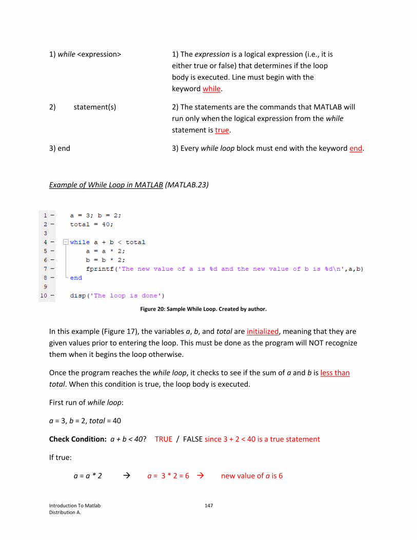
Introduction To Matlab 147 Distribution A.
Figure 20: Sample While Loop. Created by author.
1) while <expression> 1) The expression is a logical expression (i.e., it is
either true or false) that determines if the loop
body is executed. Line must begin with the
keyword while.
2) statement(s) 2) The statements are the commands that MATLAB will
run only when the logical expression from the while
statement is true.
3) end 3) Every while loop block must end with the keyword end.
Example of While Loop in MATLAB (MATLAB.23)
In this example (Figure 17), the variables a, b, and total are initialized, meaning that they are
given values prior to entering the loop. This must be done as the program will NOT recognize
them when it begins the loop otherwise.
Once the program reaches the while loop, it checks to see if the sum of a and b is less than
total. When this condition is true, the loop body is executed.
First run of while loop:
a = 3, b = 2, total = 40
Check Condition: a + b < 40? TRUE / FALSE since 3 + 2 < 40 is a true statement
If true:
a = a * 2 a = 3 * 2 = 6 new value of a is 6

Introduction To Matlab 148 Distribution A.
b = b * 2 b = 2 * 2 = 4 new value of b is 4
fprintf(…)
Once the body is completed, the program returns to the while loop statement and checks to
see if a + b < 40 is true for the new values of a and b. The program will continue this process
until this condition is false.
Here is what the example would look like as a flowchart (Figure 18):
Example 1 (MATLAB.23)
Determine the number of times each string will be printed in each script.
A)
‘Hola! Como estas?’ will be displayed 5 times.
B)
a = 12
b = 8 a = 24
b = 16
a = 12 * 2 = 24
b = 8 * 2 = 16
FalTr
True
a = 3 * 2 = 6
b = 2 * 2 = 4
a = 3, b = 2
total = 40
(Initialize)
Condition:
a + b < total?
a = 6
b = 4
End While
Loop
Condition:
a + b < total?
a = 6 * 2 = 12
b = 4 * 2 = 8
Condition:
a + b < total? Condition:
a + b < total?
True True False
Figure 21: While Loop Flowchart Example. Created by author.

Introduction To Matlab 149 Distribution A.
‘Hello World!’ will be displayed 7 times.
Example 2 (MATLAB.23)
Determine the number of times the string will be printed in the following script.
Why does the script act the way that it does? Explain.
The word ‘Loop’ will keep being displayed and never stop (this is called an infinite
loop). In this script, n must be greater than -2 for the loop to execute. Since n is initialized at 3
and 1 is added to n in the loop body, n’s value will never be below -2. Therefore, the while
statement (n > -2) will never be false, and the loop body will continuously be executed.
Example 3 (MATLAB.23)
What values will the following code print?
The code will print the values of a: 2, 6, 24, 120
Example 4 (MATLAB.24)
Use a while loop to solve each of the following problems.
A) Create a script that asks the user to input a value that is greater than 0. The script should
keep asking until a valid number is entered.

Introduction To Matlab 150 Distribution A.
B) Create a script that asks the user to enter two numbers and determines if the sum of the
numbers is even. An even number is one that is divisible by 2. The script should continue asking
for two numbers until their sum is even.
NOTE: You will need to use the b = mod(a,m) mathematical function (mod is short for modular
arithmetic). Mod calculates the remainder of a / m.
Examples:
mod(10,2) = 0 mod(10,3) = 1 mod(8,3) = 2 mod(125,6) = 5
C) Create a number guess game where a random integer from 1 to 20 is chosen, and the player
gets a maximum of three chances to guess the correct number. After each guess, the player
should receive feedback that tells them whether their guess was too low or too high. The
program should congratulate the player if they guess the correct number within the guess limit;
and the program should tell the player what number it had chosen if three incorrect guesses
have been made.
NOTE: To generate a random integer, use the randi(imax) function of MATLAB. The function
works by replacing imax with a positive integer value. The program will then select a random
integer between 1 and the value imax is equal to.
Example: a = randi(10) The value of a will be number selected randomly from 1 to 10.

Introduction To Matlab 151 Distribution A.
1.62.2. PRACTICE PROBLEMS
Practice Problems
1) Determine the number of times each string will print in the following scripts.
A)
‘STEM for the win!’ will be displayed 7 times.

Introduction To Matlab 152 Distribution A.
B)
‘Tricky’ will be displayed 4 times.
C)
Nothing is displayed since g is never less than h.
D)
‘How long does this go?’ will be constantly displayed (infinite loop).
2) Use a while loop to solve each of the following problems.
A) Create a script that displays the consecutive integers from 10 to 20.
B) Create a script that asks the user to enter two numbers and determines if the difference of
the numbers is a multiple of 6 (e.g., 6, 12, 18, 24… are multiples of 6). The script should
continue asking for two numbers until their difference is a multiple of 6.

Introduction To Matlab 153 Distribution A.
3) Create a game of rock-paper-scissors in MATLAB. Here are the requirements:
Utilize a while loop to determine when the game is over
Player should be able to choose rock, paper, or scissors on his/her turn
o NOTE: You may use numeric values to represent each item (e.g., “Press 1 for
rock,…”), but be sure to communicate this clearly to players through your
program
The computer will randomly pick rock, paper, or scissors for each round
The program should compare the choices made by the player and computer to see who
wins the round
o Rules: rock beats scissors, paper beats rock, scissors beat paper
One point is awarded to the player who wins a round
The game is over when either the player or computer earns three points
When the game is over, a message should display based on whether a player won or lost
o Example: “Congratulations!” or “Nice try!”
Your program will require the use of a while loop, conditional statements, input functions, and
other topics covered throughout the previous lessons. Good luck!
There are many possible ways this program could be created. Here is one possible solution.

Introduction To Matlab 154 Distribution A.
1.63. RESOURCES
1. Mathworks®/MATLAB® Official Support Page:
https://www.mathworks.com/help/matlab/
2. An Introduction to Solving Engineering Problems with MATLAB® e-book:
https://www.ck12.org/book/Engineering%3A-An-Introduction-to-Solving-Engineering-
Problems-with-Matlab/
1.64. IMAGE CREDITS
All images are screenshots taken by the author from The MathWorks©,Inc.: MATLAB© R2018a,
including all Command Windows provided throughout.