Introduction to Materialized Views In Teradata - · PDF fileIntroduction to Materialized Views...

Introduction to Materialized Views In Teradata

By: Grace Au and Curt Ellmann

Date: 10/25/2002 541-0003506B01

Abstract: Materialized views are implemented as join indexes in Teradata. Join in-dexes can be used to improve the performance of queries at the expense of update

performance and increased storage requirements. Teradata supports a variety of join indexes including aggregate join indexes, single-table and multi-table join in-dexes, and sparse join indexes. Join indexes can be used in conjunction with base

tables if the join index does not completely contain the columns in the select list or the selection condition. A number of techniques used to improve the performance of

maintenance for join indexes are described.

This document, and the information contained herein, are the exclusive properties of NCR Corporation. In no case shall this document or its contents be reproduced or copied by any means, in whole or in part, or disseminated outside of the company, without prior written permission of a company officer.

Copyright 2002 by NCR Corporation

Teradata Materialized Views

[This page intentionally left blank]


(10/25/02) Copyright © 2002 NCR 1

Table of Contents

1. Introduction........................................................................2

2. Join Indexes in Teradata .......................................................3

2.1.1. Creation Language ................................................................................................4

2.1.2. Maintenance.........................................................................................................4

2.1.3. Coverage Algorithm...............................................................................................5

2.1.4. Physical Structure of a Join Index.............................................................................7

3. Join Index Maintenance Improvements in V2R5.........................9

3.1. Improvement 1: Avoid Maintenance....................................................... 9

3.2. Improvement 2: Reduce Lock Granularity..............................................10

3.3. Improvement 3: Improve un-matching row maintenance..........................14

3.4. Improvement 4: Improve Aggregate Join Index Maintenance ....................16

4. Query Rewrite Improvements in V2R5 ................................... 18

5. What can Join Indexes be used for? ...................................... 20

5.1.1. Redistributing.....................................................................................................20

5.1.2. Joins.................................................................................................................20

5.1.3. Aggregate Join Indexes ........................................................................................21

5.1.4. Sparse Join Indexes.............................................................................................21

5.1.5. Join Indexes to Cover Parameterized Queries ...........................................................22

5.1.6. Partial coverage ..................................................................................................23

5.1.7. Outer Join Join Indexes........................................................................................24

5.2. What is the cost?...............................................................................25

5.3. Summary .........................................................................................26

6. Glossary........................................................................... 27

7. References ....................................................................... 29

Introduction to Materialized Views In Teradata (541-0003506B01)

2 Copyright © 2002 NCR

1. Introduction

A materialized view (MV) is a cross between a view and an index. It is like a view in that it is created using a query to specify the struc-ture, composition and source of the contents. It is like an index in the way that it is used automatically by the database system to improve the performance of a query. Teradata refers to the materialized view structure by the term "Join Index", a name that reflects its similarity to indexes. We will use the terms “materialized view” and “join index” interchangeably in this document.

Since the decision whether or not to use the join index to answer a query is left up to the database system, it is critical that the system produce the same answer whether or not the join index is chosen. This principal is followed automatically by Teradata. There are other categories of materialized views in other products that do not follow this principle. Some products require that a materialized view update be performed in order to synchronize the materialized view with recent updates to the base table. This is an extra step not required in Tera-data.

From the user's perspective, a join index or materialized view works just like an index. Both are created to improve the performance of da-tabase operations. Whether the index or join index is used, the an-swer is consistent. The only difference is in the amount of time it takes to get the answer. Both indexes and join indexes are main-tained automatically by the DBMS.


(10/25/02) Copyright © 2002 NCR 3

2. Join Indexes in Teradata

The Teradata database system supports creation of materialized views through the CREATE JOIN INDEX statement in Teradata SQL. The form of the statement is

CREATE JOIN INDEX <JI name> AS <sql-select-query> <Indexes>;

Where the sql-select-query is a query written in standard SQL with se-lections, joins or aggregates on base tables or views. Indexes allows for the specification of secondary indexes and a primary index so the join index can be hash-distributed based on a column different from any of the base tables.

There are some restrictions on the kinds of queries that can be used to specify a join index. These restrictions have to do mostly with query complexity. Queries containing subqueries, for example, cannot be used in join indexes. A large class of queries including aggregates, queries containing constant conditions in the WHERE clause, inner and outer joins are all supported.

In Teradata, join indexes are always maintained to be up to date with changes to the tables they are based upon, just like an index. You never need to be concerned about queries running against "stale" data when join indexes are used. The ability to maintain materialized views in an up-to-date form during updates to the base tables is one of the features that sets Teradata apart from other database systems.

Join Indexes are used to answer queries when the Teradata optimizer determines that a plan involving a join index will be faster than an al-ternative plan. There is no need (or ability, even!) for a database user to explicitly know of, or specify a join index when formulating a data-base query. The cost-based optimizer in Teradata evaluates the op-tions for query execution, including the use of one or more join in-dexes, and chooses the plan with the lowest cost.

There are 3 main questions that need to be answered to understand the power of the materialized view implementation in a database sys-tem.

• What is the power of the MV creation language?



• What is the approach to maintenance of the MV?

• What is the power of the coverage algorithm that the system uses to decide if a MV can be used to answer a query?

2.1.1. Creation Language

The power of the MV creation language determines what kind of join indexes can be created. The Teradata join index allows a broad range of constructs in the specification of a join index

• Joins. Both inner and outer joins are supported. Join index que-ries can join 2 or more tables, and can support complex join conditions. Currently, only equi-joins are permitted.

• Aggregates. Join indexes can be created with aggregates SUM and COUNT in the select list. These aggregates can be combined with a join, or the aggregates can be formed from a single table. The GROUP BY clause is supported which improves the versatility of the join index. Aggregate join indexes that contain SUM and COUNT aggregates on a single column can be used for queries that contain an AVG aggregate on the same column.

• Sparse Indexes. Rows can be selected to be included in (or ex-cluded from) the MV based on constant conditions specified in the WHERE clause of the join index creation DDL statement. Columns can be included in the join index using the standard Teradata SQL query syntax.

• Redistribution. The join index can be hash-distributed on any column(s) using the PRIMARY INDEX clause of the create join in-dex DDL statement.

2.1.2. Maintenance

The tables that are referenced in join indexes are referred to as base tables of the join index. A single table may be the base table for sev-eral join indexes. When a base table is updated, a join index may need to be updated to maintain its consistency with the contents of the real data tables. The amount of time required to perform the update depends on the complexity of the join index, number of joins, aggre-gates, etc.


(10/25/02) Copyright © 2002 NCR 5

In Teradata join index maintenance is performed whenever base tables are updated. This guarantees that the Teradata system always gives consistent and correct answers regardless of whether a join index is used in the query evaluation plan.

The maintenance operations on join indexes are the "cost" side of the "cost benefit" equation associated with materialized views. The objec-tive in implementing JI maintenance, is to minimize the cost associ-ated with updating the base tables included in a join index. One opti-mization that Teradata uses is to try to avoid performing maintenance when it is not necessary. Teradata uses the coverage algorithm to help determine whether to update a join index following a base table update. The expression describing the modified or inserted rows is compared with the join index expression to see if there is any overlap between the rows modified in the base table, and the contents of the join index. If there is no overlap, the maintenance step can be skipped.

When maintenance must be performed, Teradata uses 2 approaches to improve the efficiency of the maintenance operation. The first ap-proach is to map the update (or insert or delete) query directly onto the join index structure, and evaluate it. Since join indexes are stored in the same structure as tables, this is a straight-forward process. The second approach is to materialize the affected rows in a temporary ta-ble, and use the rows as a guide to maintain the join index. Mainte-nance is described in greater detail in sections 3.0 and 5.2.

2.1.3. Coverage Algorithm

The Coverage Algorithm is the process used by the database system to determine if a join index can be used to compute the answer to a query. A join index is said to "cover" a query if the query predicate specifies a set of rows that are a subset of the rows in the join index. The coverage algorithm is combined with the cost based optimization to find join indexes that can be used to improve the performance of a query. In the event that there is more than one join index, the cover-age algorithm decides which index or indexes can be used. The opt i-mizer's traditional costing function then decides which, if any, of the join indexes give the lowest cost plan for the query. The Teradata



coverage algorithm is powerful and flexible, analyzing the query and join index expressions to decide if the join index can be applied. A US patent application has been submitted for the Teradata coverage algo-rithm.

The Teradata coverage algorithm works by decomposing the query predicate, and the join index predicate into terms containing column conditions connected by ANDs or ORs. These terms are tested recur-sively according to the corresponding logic regarding ANDed or ORed conditions in query and join index respectively. For example, if the conditions in a query are ORed together, the test determines if all the terms in the query are contained in the join index predicate. For ANDed terms, only one of the terms in the query must specify a set contained in the join index.

For a simple example, suppose that we have a join index CREATE JOIN INDEX JI0 AS SELECT A, B FROM T1 WHERE A > 10

And a query SELECT A, B FROM T1 WHERE A > 20;

In this example, the JI0 join index will cover the query since the term A > 20 defines a set of rows that is completely contained in the set of rows defined by the term A > 10.

For a slightly more complex example, suppose that we have a join in-dex

CREATE JOIN INDEX JI1 AS SELECT EMPID, EMP.NAME, STORENO, STORE.STATE FROM EMP, STORE WHERE EMP.STOREID = STORE.STOREID AND STORE.STATE IN ('NE', 'CA', 'WI');

And a query SELECT EMP.NAME, STORE.STATE FROM EMP, STORE WHERE EMP.STOREID = STORE.STOREID AND (STORE.STATE = 'CA' OR STORE.STATE = 'WI');


(10/25/02) Copyright © 2002 NCR 7

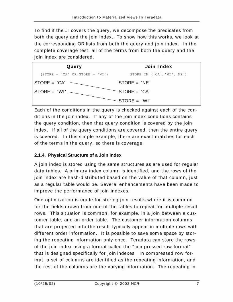
To find if the JI covers the query, we decompose the predicates from both the query and the join index. To show how this works, we look at the corresponding OR lists from both the query and join index. In the complete coverage test, all of the terms from both the query and the join index are considered.

Query

(STORE = 'CA' OR STORE = 'WI')

Join Index

STORE IN ('CA','WI','NE')

STORE = 'CA' STORE = 'NE'

STORE = 'WI' STORE = 'CA'

STORE = 'WI'

Each of the conditions in the query is checked against each of the con-ditions in the join index. If any of the join index conditions contains the query condition, then that query condition is covered by the join index. If all of the query conditions are covered, then the entire query is covered. In this simple example, there are exact matches for each of the terms in the query, so there is coverage.

2.1.4. Physical Structure of a Join Index

A join index is stored using the same structures as are used for regular data tables. A primary index column is identified, and the rows of the join index are hash-distributed based on the value of that column, just as a regular table would be. Several enhancements have been made to improve the performance of join indexes.

One optimization is made for storing join results where it is common for the fields drawn from one of the tables to repeat for multiple result rows. This situation is common, for example, in a join between a cus-tomer table, and an order table. The customer information columns that are projected into the result typically appear in multiple rows with different order information. It is possible to save some space by stor-ing the repeating information only once. Teradata can store the rows of the join index using a format called the “compressed row format” that is designed specifically for join indexes. In compressed row for-mat, a set of columns are identified as the repeating information, and the rest of the columns are the varying information. The repeating in-



formation columns are stored 1 time for each set of rows that share the same column values for the repeating columns.

If you know that the join index contains groups of rows with repeating information, then the join index creation can specify “repeating groups” showing the repeating columns in parentheses. The column list is specified as 2 groups of columns, with each group in parenthe-ses. The first group contains the repeating columns, and the second group contains the non-repeating columns.

Join indexes can be stored using a value-ordered structure so the rows are ordered by value of a 4-byte column. This structure provides bet-ter performance for queries that contain selection constraints on the value ordering column. For example, suppose that it is a common task to look up sales information by sale_date. You can create a join index on the sales table and order it by sale_date. The benefit is that que-ries that select sales by sale_date only need to access those data blocks that contain the value or range of values that the queries spec-ify.

In Teradata, join indexes can also take advantage of Fallback protec-tion. In the same way that fallback allows queries to proceed when an AMP is down by providing an online, partitioned replica of a base table, fallback protection can also be used with join indexes to allow queries and updates to proceed on fallback protected join indexes.


(10/25/02) Copyright © 2002 NCR 9

3. Join Index Maintenance Improvements in V2R5

A very important component of the overall performance of the Join In-dex feature in Teradata is the performance of the maintenance opera-tion for join indexes. As ment ioned in section 2.1.2, a join index maintenance operation must be initiated whenever an update (repre-sented by SQL INSERT, UPDATE, or DELETE statements) is made to a JI base table. In V2R5, Teradata adds a number of new optimizations to make the required maintenance operations run as fast as possible.

3.1. Improvement 1: Avoid Maintenance

The first optimization that can be done for maintenance is a test for intersection between the set of rows involved in the update and the set of rows in the join index. Teradata performs this test using the same algorithm that is used for join index coverage testing. If the update affects any of the rows from the base table that are used to form the join index, then the maintenance operations are added to the query plan for the update query. If the update does not affect the join index, then the maintenance steps are not added to the plan. For example, consider the following aggregate join index:

CREATE JOIN INDEX JX2 AS SELECT COUNT(*)(FLOAT, NAMED CountStar ),

CURT.A1.I , SUM(CURT.A1.J )(FLOAT, NAMED JJ )

FROM A1 WHERE A1.I > 10 GROUP BY A1.I PRIMARY INDEX ( I );

And the update: Delete a1 from a2 where a1.i = a2.k and a2.k <= 11; Explanation ----------------------------------------------------------------------- 1) First, we lock a distinct CURT."pseudo table" for write on a RowHash to prevent global deadlock for CURT.jx2. 2) Next, we lock a distinct CURT."pseudo table" for write on a RowHash to prevent global deadlock for CURT.a1. 3) We lock a distinct CURT."pseudo table" for read on a RowHash to prevent global deadlock for CURT.a2. 4) We lock CURT.jx2 for write, we lock CURT.a1 for write, and we lock CURT.a2 for read. 5) We execute the following steps in parallel. 1) We do an all-AMPs DELETE from CURT.jx2 by way of a traversal of index # 192 with a residual condition of ("(CURT.jx2.i <=



11) AND ((CURT.jx2.i = k) AND (k <= 11 ))"). 2) We do an all-AMPs MERGE DELETE to CURT.a1 from CURT.a2 by way of a RowHash match scan. 6) Finally, we send out an END TRANSACTION step to all AMPs involved in processing the request. -> No rows are returned to the user as the result of statement 1.

First, note that the predicate "JX2.i <= 11" was added by the transi-tive closure computation that is done for all queries processed by the system. Transitive closure provides more opportunities to avoid un-necessary maintenance operations. Second, note that the rows are removed from both the join index and the base table in step 5.

The following update cannot affect the join index, so there are no maintenance operations added to the plan for this update. delete a1 from a2 where a1.i = a2.k and a2.k < 10; Explanation ----------------------------------------------------------------------- 1) First, we lock a distinct CURT."pseudo table" for write on a RowHash to prevent global deadlock for CURT.a1. 2) Next, we lock a distinct CURT."pseudo table" for read on a RowHash to prevent global deadlock for CURT.a2. 3) We lock CURT.a1 for write, and we lock CURT.a2 for read. 4) We do an all-AMPs MERGE DELETE to CURT.a1 from CURT.a2 by way of a RowHash match scan. 5) Finally, we send out an END TRANSACTION step to all AMPs involved in processing the request. -> No rows are returned to the user as the result of statement 1.

Note that a transitive closure computation is necessary to determine that the join index JX2 will not be affected by this update since, by transitive closure, if a2.k < 10 and a1.i = a2.k, then a1.i < 10. The set of rows where a1.i < 10 is disjoint from the set where a1.i > 10.

3.2. Improvement 2: Reduce Lock Granularity

When a large number of rows must be changed in a join index, it is most efficient to lock the entire table, and perform the update. How-ever, while the table is locked, all other transactions that need to ac-cess the table must wait until the lock is released. Table level write locks can be replaced with row hash write locks in some cases. If a small number of rows are being updated, then it may be better to ac-quire locks for only those rows that are being updated. Doing so al-lows some improved concurrency on the table being updated. By us-ing statistics, it is possible to determine when it is advantageous to


(10/25/02) Copyright © 2002 NCR 11

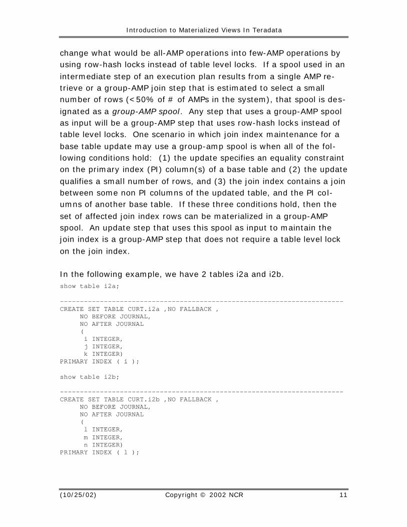
change what would be all-AMP operations into few-AMP operations by using row-hash locks instead of table level locks. If a spool used in an intermediate step of an execution plan results from a single AMP re-trieve or a group-AMP join step that is estimated to select a small number of rows (<50% of # of AMPs in the system), that spool is des-ignated as a group-AMP spool. Any step that uses a group-AMP spool as input will be a group-AMP step that uses row-hash locks instead of table level locks. One scenario in which join index maintenance for a base table update may use a group-amp spool is when all of the fol-lowing conditions hold: (1) the update specifies an equality constraint on the primary index (PI) column(s) of a base table and (2) the update qualifies a small number of rows, and (3) the join index contains a join between some non PI columns of the updated table, and the PI col-umns of another base table. If these three conditions hold, then the set of affected join index rows can be materialized in a group-AMP spool. An update step that uses this spool as input to maintain the join index is a group-AMP step that does not require a table level lock on the join index.

In the following example, we have 2 tables i2a and i2b. show table i2a; ----------------------------------------------------------------------- CREATE SET TABLE CURT.i2a ,NO FALLBACK , NO BEFORE JOURNAL, NO AFTER JOURNAL ( i INTEGER, j INTEGER, k INTEGER) PRIMARY INDEX ( i ); show table i2b; ----------------------------------------------------------------------- CREATE SET TABLE CURT.i2b ,NO FALLBACK , NO BEFORE JOURNAL, NO AFTER JOURNAL ( l INTEGER, m INTEGER, n INTEGER) PRIMARY INDEX ( l );



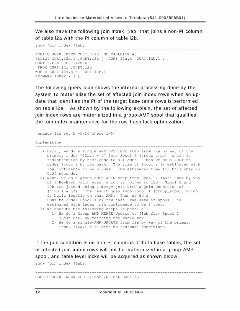
We also have the following join index, jiab, that joins a non-PI column of table i2a with the PI column of table i2b. show join index jiab; ----------------------------------------------------------------------- CREATE JOIN INDEX CURT.jiab ,NO FALLBACK AS SELECT CURT.i2a.i ,CURT.i2a.j ,CURT.i2a.k ,CURT.i2b.l , CURT.i2b.m ,CURT.i2b.n FROM CURT.i2a ,CURT.i2b WHERE CURT.i2a.j = CURT.i2b.l PRIMARY INDEX ( j );

The following query plan shows the internal processing done by the system to materialize the set of affected join index rows when an up-date that identifies the PI of the target base table rows is performed on table i2a. As shown by the following explain, the set of affected join index rows are materialized in a group-AMP spool that qualifies the join index maintenance for the row-hash lock optimization. update i2a set k =k+10 where i=5; Explanation ----------------------------------------------------------------------- 1) First, we do a single-AMP RETRIEVE step from i2a by way of the primary index "i2a.i = 5" into Spool 2 (group_amps), which is redistributed by hash code to all AMPs. Then we do a SORT to order Spool 2 by row hash. The size of Spool 2 is estimated with low confidence to be 2 rows. The estimated time for this step is 0.56 seconds. 2) Next, we do a group-AMPs JOIN step from Spool 2 (Last Use) by way of a RowHash match scan, which is joined to i2b. Spool 2 and i2b are joined using a merge join with a join condition of ("i2b.l = j"). The result goes into Spool 1 (group_amps), which is built locally on that AMP. Then we do a SORT to order Spool 1 by row hash. The size of Spool 1 is estimated with index join confidence to be 2 rows. 3) We execute the following steps in parallel. 1) We do a Group AMP MERGE Update to jiab from Spool 1 (Last Use) by matching the whole row. 2) We do a single-AMP UPDATE from i2a by way of the primary index "i2a.i = 5" with no residual conditions.

If the join condition is on non-PI columns of both base tables, the set of affected join index rows will not be materialized in a group-AMP spool, and table level locks will be acquired as shown below. show join index jiab2; ----------------------------------------------------------------------- CREATE JOIN INDEX CURT.jiab2 ,NO FALLBACK AS


(10/25/02) Copyright © 2002 NCR 13

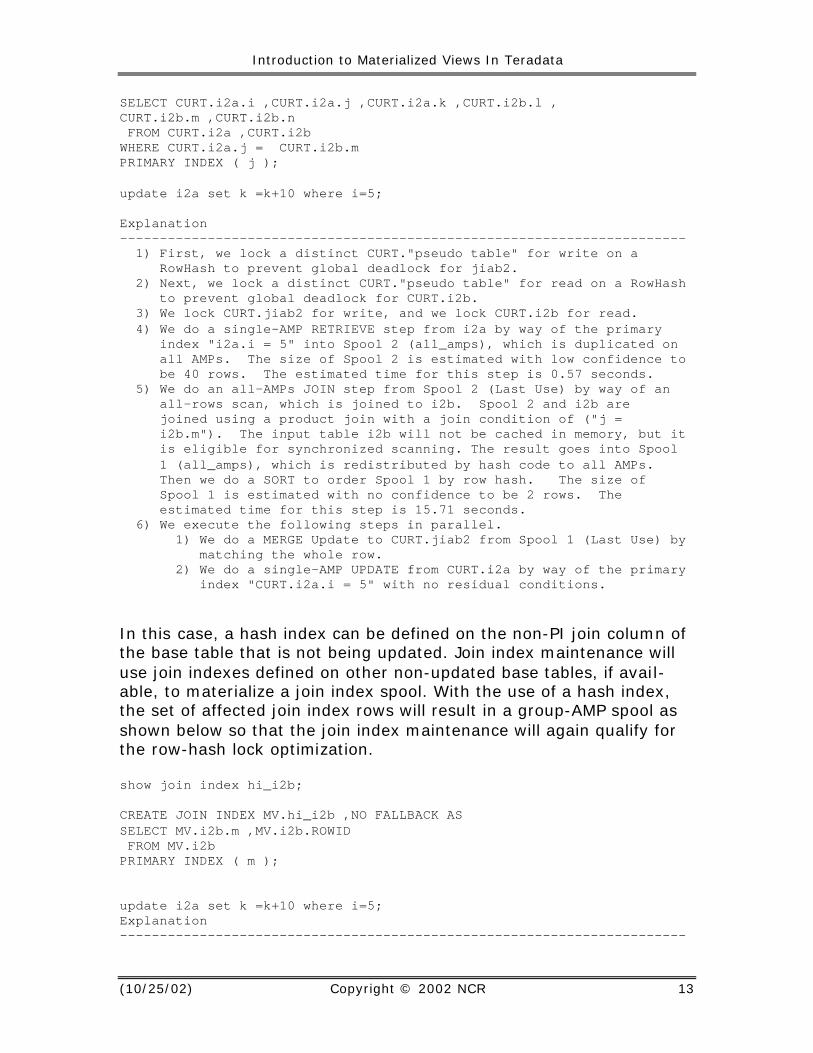
SELECT CURT.i2a.i ,CURT.i2a.j ,CURT.i2a.k ,CURT.i2b.l , CURT.i2b.m ,CURT.i2b.n FROM CURT.i2a ,CURT.i2b WHERE CURT.i2a.j = CURT.i2b.m PRIMARY INDEX ( j ); update i2a set k =k+10 where i=5; Explanation ----------------------------------------------------------------------- 1) First, we lock a distinct CURT."pseudo table" for write on a RowHash to prevent global deadlock for jiab2. 2) Next, we lock a distinct CURT."pseudo table" for read on a RowHash to prevent global deadlock for CURT.i2b. 3) We lock CURT.jiab2 for write, and we lock CURT.i2b for read. 4) We do a single-AMP RETRIEVE step from i2a by way of the primary index "i2a.i = 5" into Spool 2 (all_amps), which is duplicated on all AMPs. The size of Spool 2 is estimated with low confidence to be 40 rows. The estimated time for this step is 0.57 seconds. 5) We do an all-AMPs JOIN step from Spool 2 (Last Use) by way of an all-rows scan, which is joined to i2b. Spool 2 and i2b are joined using a product join with a join condition of ("j = i2b.m"). The input table i2b will not be cached in memory, but it is eligible for synchronized scanning. The result goes into Spool 1 (all_amps), which is redistributed by hash code to all AMPs. Then we do a SORT to order Spool 1 by row hash. The size of Spool 1 is estimated with no confidence to be 2 rows. The estimated time for this step is 15.71 seconds. 6) We execute the following steps in parallel. 1) We do a MERGE Update to CURT.jiab2 from Spool 1 (Last Use) by matching the whole row. 2) We do a single-AMP UPDATE from CURT.i2a by way of the primary index "CURT.i2a.i = 5" with no residual conditions. In this case, a hash index can be defined on the non-PI join column of the base table that is not being updated. Join index maintenance will use join indexes defined on other non-updated base tables, if avail-able, to materialize a join index spool. With the use of a hash index, the set of affected join index rows will result in a group-AMP spool as shown below so that the join index maintenance will again qualify for the row-hash lock optimization. show join index hi_i2b; CREATE JOIN INDEX MV.hi_i2b ,NO FALLBACK AS SELECT MV.i2b.m ,MV.i2b.ROWID FROM MV.i2b PRIMARY INDEX ( m ); update i2a set k =k+10 where i=5; Explanation -----------------------------------------------------------------------



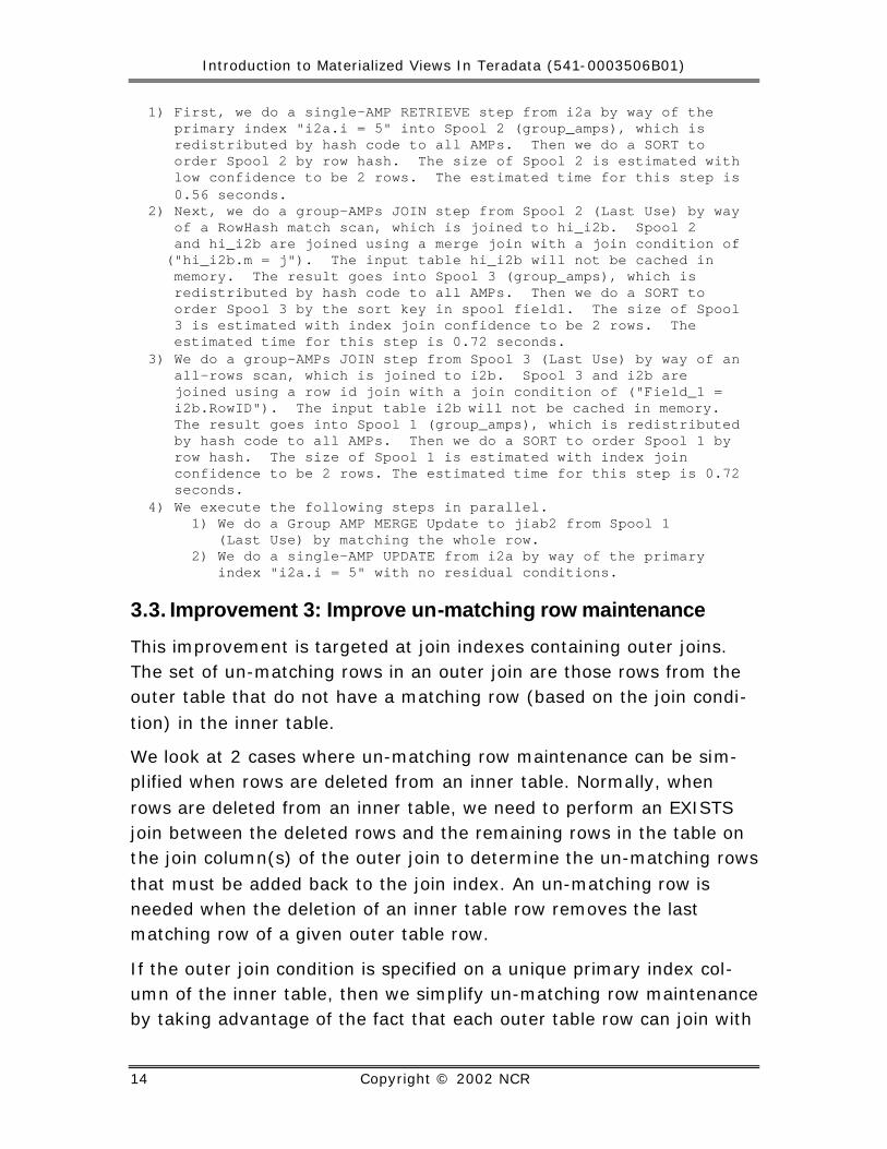
1) First, we do a single-AMP RETRIEVE step from i2a by way of the primary index "i2a.i = 5" into Spool 2 (group_amps), which is redistributed by hash code to all AMPs. Then we do a SORT to order Spool 2 by row hash. The size of Spool 2 is estimated with low confidence to be 2 rows. The estimated time for this step is 0.56 seconds. 2) Next, we do a group-AMPs JOIN step from Spool 2 (Last Use) by way of a RowHash match scan, which is joined to hi_i2b. Spool 2 and hi_i2b are joined using a merge join with a join condition of ("hi_i2b.m = j"). The input table hi_i2b will not be cached in memory. The result goes into Spool 3 (group_amps), which is redistributed by hash code to all AMPs. Then we do a SORT to order Spool 3 by the sort key in spool field1. The size of Spool 3 is estimated with index join confidence to be 2 rows. The estimated time for this step is 0.72 seconds. 3) We do a group-AMPs JOIN step from Spool 3 (Last Use) by way of an all-rows scan, which is joined to i2b. Spool 3 and i2b are joined using a row id join with a join condition of ("Field_1 = i2b.RowID"). The input table i2b will not be cached in memory. The result goes into Spool 1 (group_amps), which is redistributed by hash code to all AMPs. Then we do a SORT to order Spool 1 by row hash. The size of Spool 1 is estimated with index join confidence to be 2 rows. The estimated time for this step is 0.72 seconds. 4) We execute the following steps in parallel. 1) We do a Group AMP MERGE Update to jiab2 from Spool 1 (Last Use) by matching the whole row. 2) We do a single-AMP UPDATE from i2a by way of the primary index "i2a.i = 5" with no residual conditions.

3.3. Improvement 3: Improve un-matching row maintenance

This improvement is targeted at join indexes containing outer joins. The set of un-matching rows in an outer join are those rows from the outer table that do not have a matching row (based on the join condi-tion) in the inner table.

We look at 2 cases where un-matching row maintenance can be sim-plified when rows are deleted from an inner table. Normally, when rows are deleted from an inner table, we need to perform an EXISTS join between the deleted rows and the remaining rows in the table on the join column(s) of the outer join to determine the un-matching rows that must be added back to the join index. An un-matching row is needed when the deletion of an inner table row removes the last matching row of a given outer table row.

If the outer join condition is specified on a unique primary index col-umn of the inner table, then we simplify un-matching row maintenance by taking advantage of the fact that each outer table row can join with


(10/25/02) Copyright © 2002 NCR 15

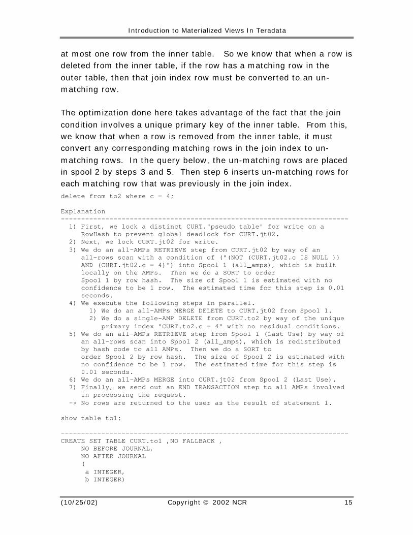
at most one row from the inner table. So we know that when a row is deleted from the inner table, if the row has a matching row in the outer table, then that join index row must be converted to an un-matching row.

The optimization done here takes advantage of the fact that the join condition involves a unique primary key of the inner table. From this, we know that when a row is removed from the inner table, it must convert any corresponding matching rows in the join index to un-matching rows. In the query below, the un-matching rows are placed in spool 2 by steps 3 and 5. Then step 6 inserts un-matching rows for each matching row that was previously in the join index. delete from to2 where c = 4; Explanation ----------------------------------------------------------------------- 1) First, we lock a distinct CURT."pseudo table" for write on a RowHash to prevent global deadlock for CURT.jt02. 2) Next, we lock CURT.jt02 for write. 3) We do an all-AMPs RETRIEVE step from CURT.jt02 by way of an all-rows scan with a condition of ("(NOT (CURT.jt02.c IS NULL )) AND (CURT.jt02.c = 4)") into Spool 1 (all_amps), which is built locally on the AMPs. Then we do a SORT to order Spool 1 by row hash. The size of Spool 1 is estimated with no confidence to be 1 row. The estimated time for this step is 0.01 seconds. 4) We execute the following steps in parallel. 1) We do an all-AMPs MERGE DELETE to CURT.jt02 from Spool 1. 2) We do a single-AMP DELETE from CURT.to2 by way of the unique primary index "CURT.to2.c = 4" with no residual conditions. 5) We do an all-AMPs RETRIEVE step from Spool 1 (Last Use) by way of an all-rows scan into Spool 2 (all_amps), which is redistributed by hash code to all AMPs. Then we do a SORT to order Spool 2 by row hash. The size of Spool 2 is estimated with no confidence to be 1 row. The estimated time for this step is 0.01 seconds. 6) We do an all-AMPs MERGE into CURT.jt02 from Spool 2 (Last Use). 7) Finally, we send out an END TRANSACTION step to all AMPs involved in processing the request. -> No rows are returned to the user as the result of statement 1. show table to1; ----------------------------------------------------------------------- CREATE SET TABLE CURT.to1 ,NO FALLBACK , NO BEFORE JOURNAL, NO AFTER JOURNAL ( a INTEGER, b INTEGER)



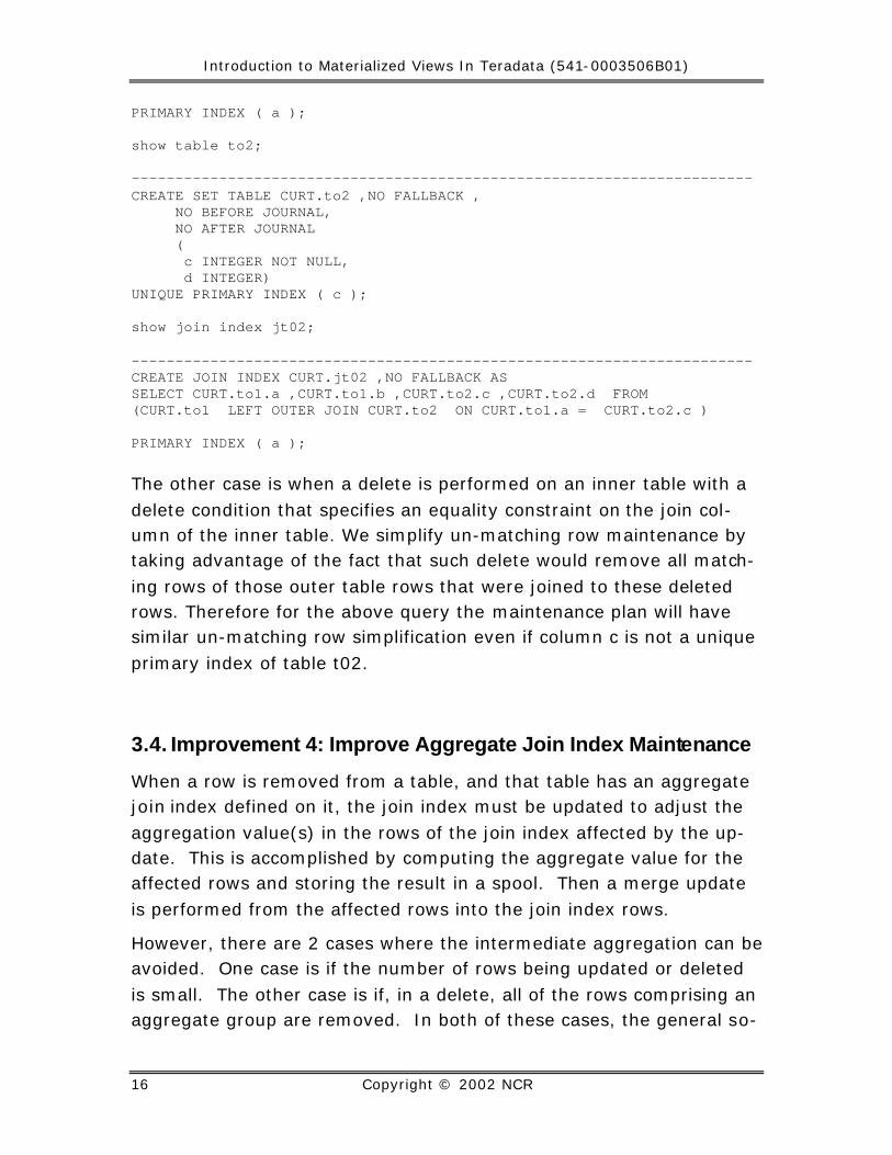
PRIMARY INDEX ( a ); show table to2; ----------------------------------------------------------------------- CREATE SET TABLE CURT.to2 ,NO FALLBACK , NO BEFORE JOURNAL, NO AFTER JOURNAL ( c INTEGER NOT NULL, d INTEGER) UNIQUE PRIMARY INDEX ( c ); show join index jt02; ----------------------------------------------------------------------- CREATE JOIN INDEX CURT.jt02 ,NO FALLBACK AS SELECT CURT.to1.a ,CURT.to1.b ,CURT.to2.c ,CURT.to2.d FROM (CURT.to1 LEFT OUTER JOIN CURT.to2 ON CURT.to1.a = CURT.to2.c ) PRIMARY INDEX ( a );

The other case is when a delete is performed on an inner table with a delete condition that specifies an equality constraint on the join col-umn of the inner table. We simplify un-matching row maintenance by taking advantage of the fact that such delete would remove all match-ing rows of those outer table rows that were joined to these deleted rows. Therefore for the above query the maintenance plan will have similar un-matching row simplification even if column c is not a unique primary index of table t02.

3.4. Improvement 4: Improve Aggregate Join Index Maintenance

When a row is removed from a table, and that table has an aggregate join index defined on it, the join index must be updated to adjust the aggregation value(s) in the rows of the join index affected by the up-date. This is accomplished by computing the aggregate value for the affected rows and storing the result in a spool. Then a merge update is performed from the affected rows into the join index rows.

However, there are 2 cases where the intermediate aggregation can be avoided. One case is if the number of rows being updated or deleted is small. The other case is if, in a delete, all of the rows comprising an aggregate group are removed. In both of these cases, the general so-


(10/25/02) Copyright © 2002 NCR 17

lution of aggregating the deleted rows, and using those to update the join index is avoided, and the delete predicate is used to identify the affected JI rows directly.



4. Query Rewrite Improvements in V2R5

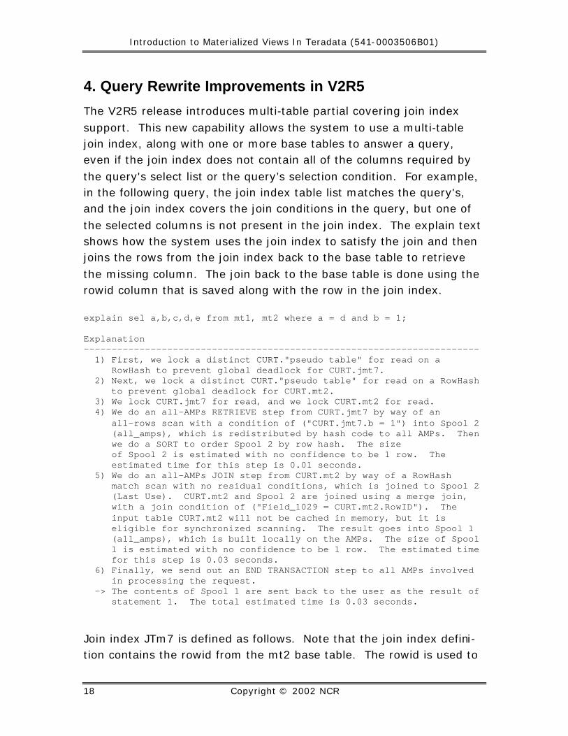
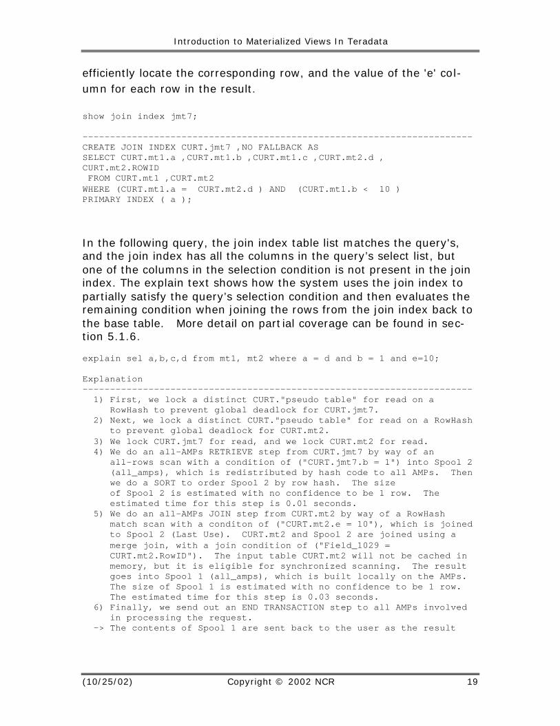
The V2R5 release introduces multi-table partial covering join index support. This new capability allows the system to use a multi-table join index, along with one or more base tables to answer a query, even if the join index does not contain all of the columns required by the query's select list or the query’s selection condition. For example, in the following query, the join index table list matches the query's, and the join index covers the join conditions in the query, but one of the selected columns is not present in the join index. The explain text shows how the system uses the join index to satisfy the join and then joins the rows from the join index back to the base table to retrieve the missing column. The join back to the base table is done using the rowid column that is saved along with the row in the join index. explain sel a,b,c,d,e from mt1, mt2 where a = d and b = 1; Explanation ----------------------------------------------------------------------- 1) First, we lock a distinct CURT."pseudo table" for read on a RowHash to prevent global deadlock for CURT.jmt7. 2) Next, we lock a distinct CURT."pseudo table" for read on a RowHash to prevent global deadlock for CURT.mt2. 3) We lock CURT.jmt7 for read, and we lock CURT.mt2 for read. 4) We do an all-AMPs RETRIEVE step from CURT.jmt7 by way of an all-rows scan with a condition of ("CURT.jmt7.b = 1") into Spool 2 (all_amps), which is redistributed by hash code to all AMPs. Then we do a SORT to order Spool 2 by row hash. The size of Spool 2 is estimated with no confidence to be 1 row. The estimated time for this step is 0.01 seconds. 5) We do an all-AMPs JOIN step from CURT.mt2 by way of a RowHash match scan with no residual conditions, which is joined to Spool 2 (Last Use). CURT.mt2 and Spool 2 are joined using a merge join, with a join condition of ("Field_1029 = CURT.mt2.RowID"). The input table CURT.mt2 will not be cached in memory, but it is eligible for synchronized scanning. The result goes into Spool 1 (all_amps), which is built locally on the AMPs. The size of Spool 1 is estimated with no confidence to be 1 row. The estimated time for this step is 0.03 seconds. 6) Finally, we send out an END TRANSACTION step to all AMPs involved in processing the request. -> The contents of Spool 1 are sent back to the user as the result of statement 1. The total estimated time is 0.03 seconds.

Join index JTm7 is defined as follows. Note that the join index defini-tion contains the rowid from the mt2 base table. The rowid is used to


(10/25/02) Copyright © 2002 NCR 19

efficiently locate the corresponding row, and the value of the 'e' col-umn for each row in the result. show join index jmt7; ----------------------------------------------------------------------- CREATE JOIN INDEX CURT.jmt7 ,NO FALLBACK AS SELECT CURT.mt1.a ,CURT.mt1.b ,CURT.mt1.c ,CURT.mt2.d , CURT.mt2.ROWID FROM CURT.mt1 ,CURT.mt2 WHERE (CURT.mt1.a = CURT.mt2.d ) AND (CURT.mt1.b < 10 ) PRIMARY INDEX ( a ); In the following query, the join index table list matches the query's, and the join index has all the columns in the query’s select list, but one of the columns in the selection condition is not present in the join index. The explain text shows how the system uses the join index to partially satisfy the query’s selection condition and then evaluates the remaining condition when joining the rows from the join index back to the base table. More detail on part ial coverage can be found in sec-tion 5.1.6. explain sel a,b,c,d from mt1, mt2 where a = d and b = 1 and e=10; Explanation ----------------------------------------------------------------------- 1) First, we lock a distinct CURT."pseudo table" for read on a RowHash to prevent global deadlock for CURT.jmt7. 2) Next, we lock a distinct CURT."pseudo table" for read on a RowHash to prevent global deadlock for CURT.mt2. 3) We lock CURT.jmt7 for read, and we lock CURT.mt2 for read. 4) We do an all-AMPs RETRIEVE step from CURT.jmt7 by way of an all-rows scan with a condition of ("CURT.jmt7.b = 1") into Spool 2 (all_amps), which is redistributed by hash code to all AMPs. Then we do a SORT to order Spool 2 by row hash. The size of Spool 2 is estimated with no confidence to be 1 row. The estimated time for this step is 0.01 seconds. 5) We do an all-AMPs JOIN step from CURT.mt2 by way of a RowHash match scan with a conditon of ("CURT.mt2.e = 10"), which is joined to Spool 2 (Last Use). CURT.mt2 and Spool 2 are joined using a merge join, with a join condition of ("Field_1029 = CURT.mt2.RowID"). The input table CURT.mt2 will not be cached in memory, but it is eligible for synchronized scanning. The result goes into Spool 1 (all_amps), which is built locally on the AMPs. The size of Spool 1 is estimated with no confidence to be 1 row. The estimated time for this step is 0.03 seconds. 6) Finally, we send out an END TRANSACTION step to all AMPs involved in processing the request. -> The contents of Spool 1 are sent back to the user as the result



5. What can Join Indexes be used for?

5.1.1. Redistributing

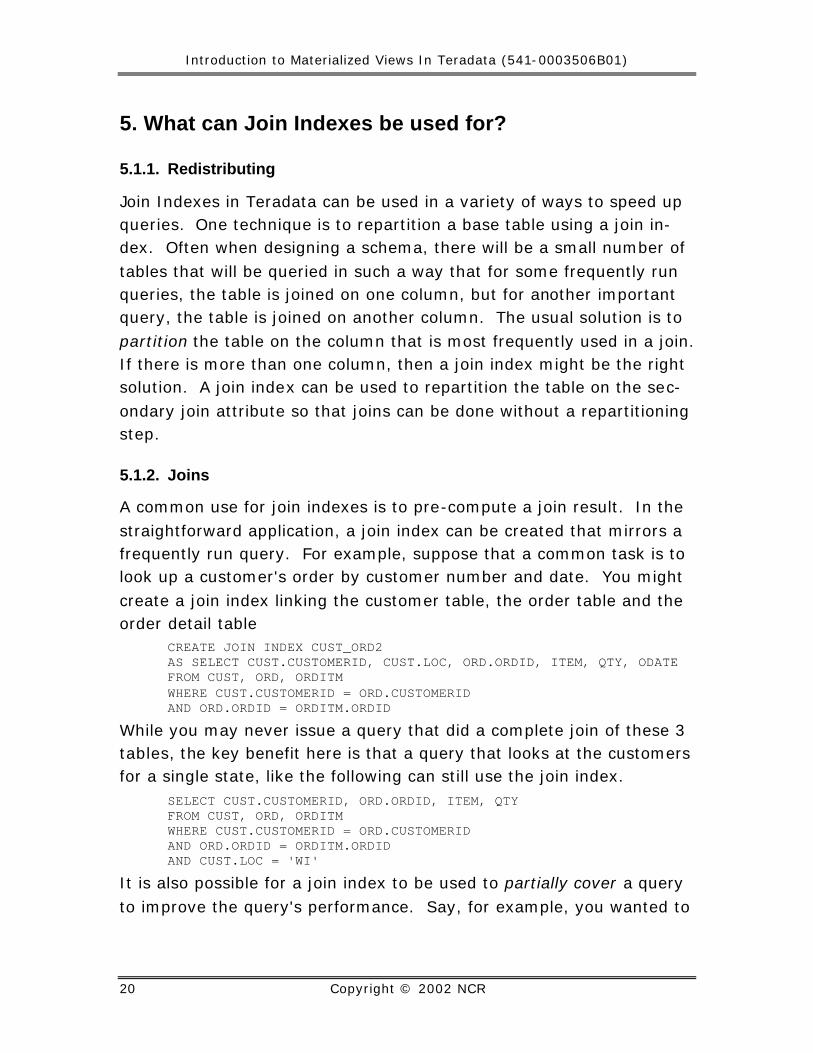
Join Indexes in Teradata can be used in a variety of ways to speed up queries. One technique is to repartition a base table using a join in-dex. Often when designing a schema, there will be a small number of tables that will be queried in such a way that for some frequently run queries, the table is joined on one column, but for another important query, the table is joined on another column. The usual solution is to partition the table on the column that is most frequently used in a join. If there is more than one column, then a join index might be the right solution. A join index can be used to repartition the table on the sec-ondary join attribute so that joins can be done without a repartitioning step.

5.1.2. Joins

A common use for join indexes is to pre-compute a join result. In the straightforward application, a join index can be created that mirrors a frequently run query. For example, suppose that a common task is to look up a customer's order by customer number and date. You might create a join index linking the customer table, the order table and the order detail table

CREATE JOIN INDEX CUST_ORD2 AS SELECT CUST.CUSTOMERID, CUST.LOC, ORD.ORDID, ITEM, QTY, ODATE FROM CUST, ORD, ORDITM WHERE CUST.CUSTOMERID = ORD.CUSTOMERID AND ORD.ORDID = ORDITM.ORDID

While you may never issue a query that did a complete join of these 3 tables, the key benefit here is that a query that looks at the customers for a single state, like the following can still use the join index.

SELECT CUST.CUSTOMERID, ORD.ORDID, ITEM, QTY FROM CUST, ORD, ORDITM WHERE CUST.CUSTOMERID = ORD.CUSTOMERID AND ORD.ORDID = ORDITM.ORDID AND CUST.LOC = 'WI'

It is also possible for a join index to be used to partially cover a query to improve the query's performance. Say, for example, you wanted to


(10/25/02) Copyright © 2002 NCR 21

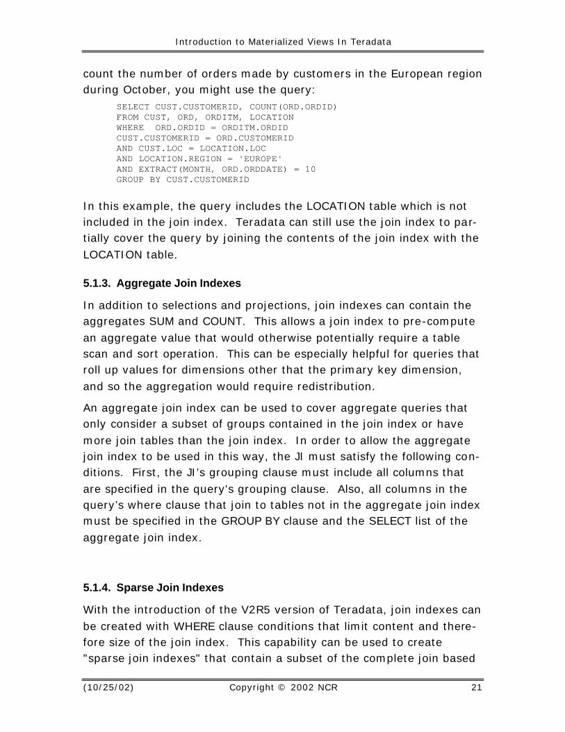
count the number of orders made by customers in the European region during October, you might use the query:

SELECT CUST.CUSTOMERID, COUNT(ORD.ORDID) FROM CUST, ORD, ORDITM, LOCATION WHERE ORD.ORDID = ORDITM.ORDID CUST.CUSTOMERID = ORD.CUSTOMERID AND CUST.LOC = LOCATION.LOC AND LOCATION.REGION = 'EUROPE' AND EXTRACT(MONTH, ORD.ORDDATE) = 10 GROUP BY CUST.CUSTOMERID

In this example, the query includes the LOCATION table which is not included in the join index. Teradata can still use the join index to par-tially cover the query by joining the contents of the join index with the LOCATION table.

5.1.3. Aggregate Join Indexes

In addition to selections and projections, join indexes can contain the aggregates SUM and COUNT. This allows a join index to pre-compute an aggregate value that would otherwise potentially require a table scan and sort operation. This can be especially helpful for queries that roll up values for dimensions other that the primary key dimension, and so the aggregation would require redistribution.

An aggregate join index can be used to cover aggregate queries that only consider a subset of groups contained in the join index or have more join tables than the join index. In order to allow the aggregate join index to be used in this way, the JI must satisfy the following con-ditions. First, the JI’s grouping clause must include all columns that are specified in the query's grouping clause. Also, all columns in the query’s where clause that join to tables not in the aggregate join index must be specified in the GROUP BY clause and the SELECT list of the aggregate join index.

5.1.4. Sparse Join Indexes

With the introduction of the V2R5 version of Teradata, join indexes can be created with WHERE clause conditions that limit content and there-fore size of the join index. This capability can be used to create "sparse join indexes" that contain a subset of the complete join based



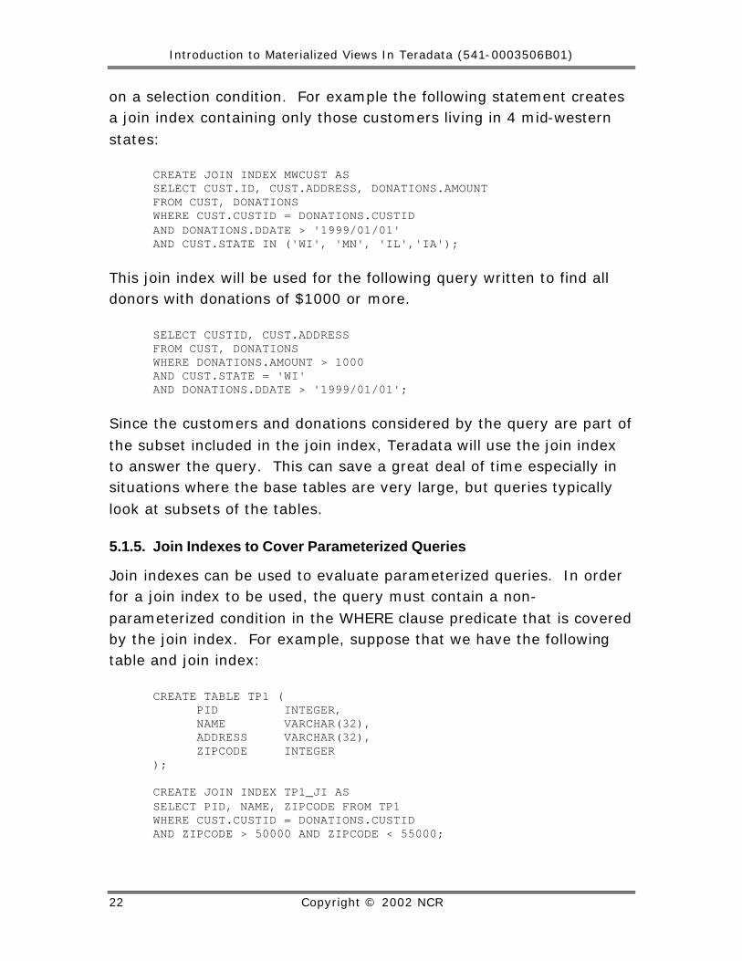
on a selection condition. For example the following statement creates a join index containing only those customers living in 4 mid-western states:

CREATE JOIN INDEX MWCUST AS SELECT CUST.ID, CUST.ADDRESS, DONATIONS.AMOUNT FROM CUST, DONATIONS WHERE CUST.CUSTID = DONATIONS.CUSTID AND DONATIONS.DDATE > '1999/01/01' AND CUST.STATE IN ('WI', 'MN', 'IL','IA');

This join index will be used for the following query written to find all donors with donations of $1000 or more.

SELECT CUSTID, CUST.ADDRESS FROM CUST, DONATIONS WHERE DONATIONS.AMOUNT > 1000 AND CUST.STATE = 'WI' AND DONATIONS.DDATE > '1999/01/01';

Since the customers and donations considered by the query are part of the subset included in the join index, Teradata will use the join index to answer the query. This can save a great deal of time especially in situations where the base tables are very large, but queries typically look at subsets of the tables.

5.1.5. Join Indexes to Cover Parameterized Queries

Join indexes can be used to evaluate parameterized queries. In order for a join index to be used, the query must contain a non-parameterized condition in the WHERE clause predicate that is covered by the join index. For example, suppose that we have the following table and join index:

CREATE TABLE TP1 ( PID INTEGER, NAME VARCHAR(32), ADDRESS VARCHAR(32), ZIPCODE INTEGER ); CREATE JOIN INDEX TP1_JI AS SELECT PID, NAME, ZIPCODE FROM TP1 WHERE CUST.CUSTID = DONATIONS.CUSTID AND ZIPCODE > 50000 AND ZIPCODE < 55000;


(10/25/02) Copyright © 2002 NCR 23

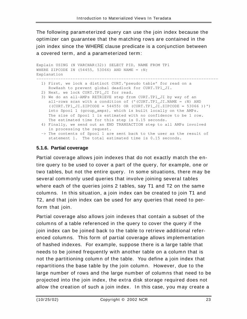
The following parameterized query can use the join index because the optimizer can guarantee that the matching rows are contained in the join index since the WHERE clause predicate is a conjunction between a covered term, and a parameterized term: Explain USING (N VARCHAR(32)) SELECT PID, NAME FROM TP1 WHERE ZIPCODE IN (54455, 53066) AND NAME = :N; Explanation --------------------------------------------------------------------------- 1) First, we lock a distinct CURT."pseudo table" for read on a RowHash to prevent global deadlock for CURT.TP1_JI. 2) Next, we lock CURT.TP1_JI for read. 3) We do an all-AMPs RETRIEVE step from CURT.TP1_JI by way of an all-rows scan with a condition of ("(CURT.TP1_JI.NAME = :N) AND ((CURT.TP1_JI.ZIPCODE = 54455) OR (CURT.TP1_JI.ZIPCODE = 53066 ))") into Spool 1 (group_amps), which is built locally on the AMPs. The size of Spool 1 is estimated with no confidence to be 1 row. The estimated time for this step is 0.15 seconds. 4) Finally, we send out an END TRANSACTION step to all AMPs involved in processing the request. -> The contents of Spool 1 are sent back to the user as the result of statement 1. The total estimated time is 0.15 seconds.

5.1.6. Partial coverage

Partial coverage allows join indexes that do not exactly match the en-tire query to be used to cover a part of the query, for example, one or two tables, but not the entire query. In some situations, there may be several commonly used queries that involve joining several tables where each of the queries joins 2 tables, say T1 and T2 on the same columns. In this situation, a join index can be created to join T1 and T2, and that join index can be used for any queries that need to per-form that join.

Partial coverage also allows join indexes that contain a subset of the columns of a table referenced in the query to cover the query if the join index can be joined back to the table to retrieve additional refer-enced columns. This form of partial coverage allows implementation of hashed indexes. For example, suppose there is a large table that needs to be joined frequently with another table on a column that is not the partitioning column of the table. You define a join index that repartitions the base table by the join column. However, due to the large number of rows and the large number of columns that need to be projected into the join index, the extra disk storage required does not allow the creation of such a join index. In this case, you may create a



join index to contain only the join column and the rowid or the unique primary index (UPI) column(s) (primary key) of the table. The join in-dex will be first joined with the other table applying any selection con-ditions that can be evaluated during the join to eliminate disqualified rows. The result of the join is stored in a temporary table and redis-tributed based on the rowid/UPI of the base table to perform a join with the base table. This join-back can happen at different points in the query plan, depending on cost. For example, the optimizer may determine that it is cheaper to perform a join with another table in-volved in the query before joining back to the base table. Partial cov-erage adds a new dimension to the usage of join indexes. A US patent application has been submitted for the Teradata partial-covering join index.

5.1.7. Outer Join Join Indexes

Join indexes can be defined with outer joins. These outer join join in-dexes can be used to cover both inner and outer join queries. To see how this is possible, consider that an outer join can be thought of as producing a result consisting of 2 sets of rows. One set corresponds to the set of “matched” rows where a row from the outer table matches one or more rows from the inner table. This set corresponds to the set of rows defined by the inner join with the same join condition. The other set of “unmatched “ rows corresponds to the rows from the outer table that do not match any rows from the inner table.

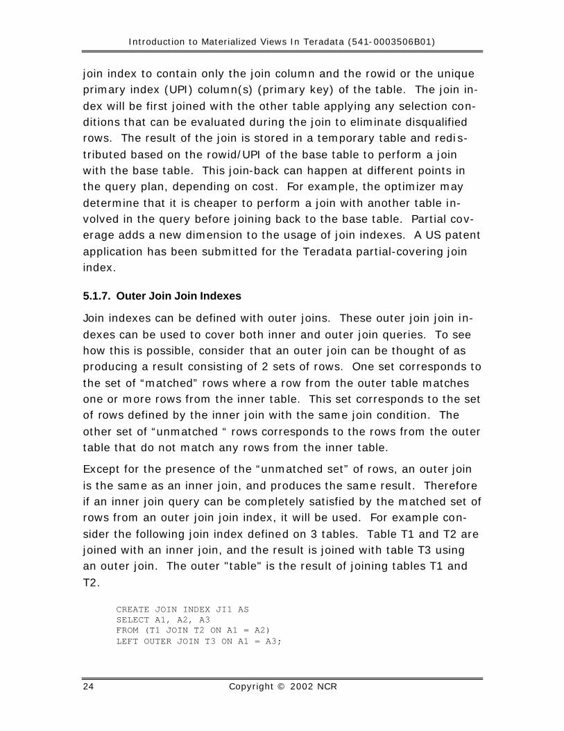
Except for the presence of the “unmatched set” of rows, an outer join is the same as an inner join, and produces the same result. Therefore if an inner join query can be completely satisfied by the matched set of rows from an outer join join index, it will be used. For example con-sider the following join index defined on 3 tables. Table T1 and T2 are joined with an inner join, and the result is joined with table T3 using an outer join. The outer "table" is the result of joining tables T1 and T2.

CREATE JOIN INDEX JI1 AS SELECT A1, A2, A3 FROM (T1 JOIN T2 ON A1 = A2) LEFT OUTER JOIN T3 ON A1 = A3;


(10/25/02) Copyright © 2002 NCR 25

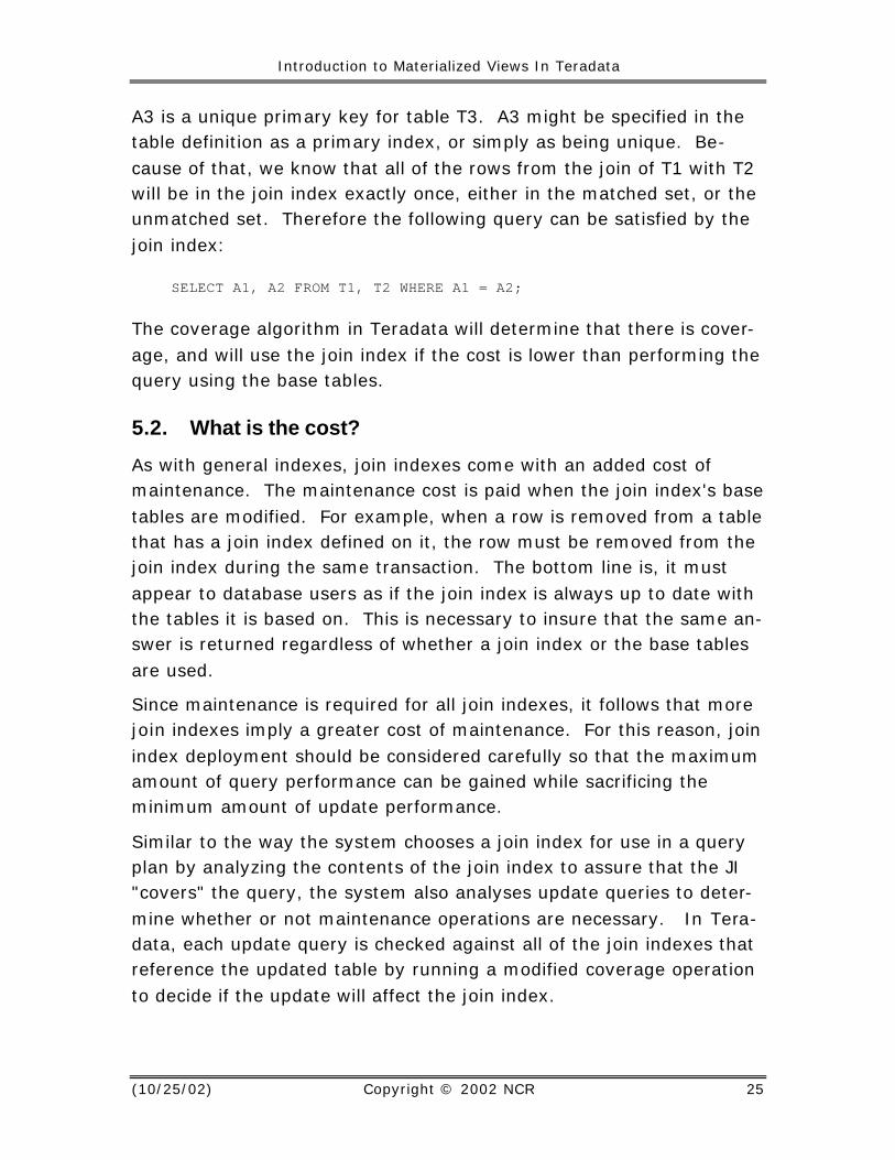
A3 is a unique primary key for table T3. A3 might be specified in the table definition as a primary index, or simply as being unique. Be-cause of that, we know that all of the rows from the join of T1 with T2 will be in the join index exactly once, either in the matched set, or the unmatched set. Therefore the following query can be satisfied by the join index:

SELECT A1, A2 FROM T1, T2 WHERE A1 = A2;

The coverage algorithm in Teradata will determine that there is cover-age, and will use the join index if the cost is lower than performing the query using the base tables.

5.2. What is the cost?

As with general indexes, join indexes come with an added cost of maintenance. The maintenance cost is paid when the join index's base tables are modified. For example, when a row is removed from a table that has a join index defined on it, the row must be removed from the join index during the same transaction. The bottom line is, it must appear to database users as if the join index is always up to date with the tables it is based on. This is necessary to insure that the same an-swer is returned regardless of whether a join index or the base tables are used.

Since maintenance is required for all join indexes, it follows that more join indexes imply a greater cost of maintenance. For this reason, join index deployment should be considered carefully so that the maximum amount of query performance can be gained while sacrificing the minimum amount of update performance.

Similar to the way the system chooses a join index for use in a query plan by analyzing the contents of the join index to assure that the JI "covers" the query, the system also analyses update queries to deter-mine whether or not maintenance operations are necessary. In Tera-data, each update query is checked against all of the join indexes that reference the updated table by running a modified coverage operation to decide if the update will affect the join index.



As an example of this, suppose that there is a table containing all of the customer records for the entire world. The table has a column that indicates the country where the customer lives. In this system, there are a large number of queries that look at customers living in the US. To improve the performance of these queries, we create a join index on the customer table selecting those customers in the US. When the customer table is updated, maintenance is only required (and per-formed) when the location column specifies US.

5.3. Summary

Join indexes use the "classic" space-time tradeoff trading disk space for storage of the join index to get improved performance for queries. Unlike many other materialized view implementations, Teradata join indexes are updated immediately and automatically when changes are made to the base tables. There is never a concern that you might be using stale data when the system chooses to use a join index in the query plan. Also, Teradata uses its sophisticated coverage testing al-gorithm to minimize the cost associated with join index maintenance.


(10/25/02) Copyright © 2002 NCR 27

6. Glossary

Compressed Row Format Join indexes are stored using the compressed row format. The format provides a saving in storage space for JIs containing repeating groups of rows where one part of the row stays constant, while the other part varies. In order to use the compressed row format, the JI creator must specify the JI columns using the com-pressed row format syntax placing parentheses '(' and ')' around both the header part and the variable part of the row. The header part is stored one time for each group of records.

Coverage Test A test that the DBMS does to determine if the rows re-quired by a query are contained in a join index. A join index covers a query if it can be shown logically that all of the rows in the query re-sult are contained in the join index.

Hashing Hashing is an operation that computes an integer from a value. The value may be any type. The hash value of a rows primary index column is used to determine where the row is physically stored.

JI Abbreviation for Jo in Index

Materialized View A materialized view is a pre-computed query result, created from an SQL query expression. In Teradata, materialized views are created using the CREATE JOIN INDEX statement. Material-ized Views can have a partitioning (i.e., primary index) different from the base table(s).

MV Abbreviation for Materialized View

Partial Coverage Partial coverage refers to the relationship between the join index and the query. If a join index partially covers a query, then the tables in the join index may be a subset of the tables referenced in the query. In order to use a join index that partially covers a query, the database system must be able to join the contents of the join in-dex with a base table to form the result. Another type of partial cov-erage refers to a join index that contains a subset of the columns ref-erenced in the query. In this case, to use the join index, the database system must join the join index with one or more tables that are con-tained in the join index in order to retrieve additional referenced col-umns.

Partition In a parallel database system, a table is partitioned so that the rows can be divided among the AMPs in the database system. One or



more columns of each table are designated as the primary index, and the value of the primary index columns are used to determine where the row should be placed. The process of partitioning is sometimes re-ferred to as hash-distribution.

Parameterized Queries A parameterized query is a query that con-tains an unbound parameter. The parameter is bound just before exe-cution. Parameterized queries can be created by ODBC sessions. The BTEQ program also allows a parameterized query to be specified with the USING syntax

Fallback Teradata technique for providing hardware failure protection by storing table rows replicated on another database system disk. If the primary disk fails, the fallback disk(s) will be used in its place.

Redistribution Redistribution is an operation that is performed on a table to change the physical location of the rows in the table. In Teradata, a row's location is determined by computing the hash value of the pri-mary index column, the hash value is determines the location where the row is stored.

Sparse Join Index A sparse join index is a JI that is created with a WHERE clause predicate containing constant conditions. Specifying a WHERE clause causes the JI to be created for a selected portion of the rows in the JI table(s).

Transitive Closure A mathematical term referring to an operation on a graph that results in a new graph where any 2 vertices of the graph that are connected by an edge to a third vertex are made to connect to each other. Teradata uses transitive closure in the optimizer to find new conditions that are implied by the conditions specified in a query. For example, if a query condition specifies A=B AND B=C, the transi-tive closure processing will add the condition A=C. Logically, if both A and C are equal to B, then A must also be equal to C.

Introduction to Materialized Views In Teradata - · PDF fileIntroduction to Materialized Views...

Documents

Transcript of Introduction to Materialized Views In Teradata - · PDF fileIntroduction to Materialized Views...