21

Chapter

Management Science

1

M01_TAYL3045_13_GE_C01.indd 21 26/10/2018 09:41

Sample

page

s

22 Chapter 1 ManageMent SCienCe

Management science is the application of a scientific approach to solving management prob-lems to help managers make better decisions. As implied by this definition, management science encompasses a number of mathematically oriented techniques that have either been developed within the field of management science or been adapted from other disciplines, such as the natu-ral sciences, mathematics, statistics, and engineering. This text provides an introduction to the techniques that make up management science and demonstrates their applications to management problems.

Management science is a recognized and established discipline in business. The applications of management science techniques are widespread, and they have been frequently credited with increasing the efficiency and productivity of business firms. In various surveys of businesses, many indicate that they use management science techniques, and most rate the results to be very good. Management science (also referred to as operations research, quantitative methods, quan-titative analysis, decision sciences, and business analytics) is part of the fundamental curriculum of most programs in business.

As you proceed through the various management science models and techniques contained in this text, you should remember several things. First, most of the examples presented in this text are for business organizations because businesses represent the main users of management sci-ence. However, management science techniques can be applied to solve problems in different types of organizations, including services, government, military, business and industry, and health care.

Second, in this text all the modeling techniques and solution methods are mathematically based. In some instances the manual, mathematical solution approach is shown because it helps one understand how the modeling techniques are applied to different problems. However, a com-puter solution is possible for each of the modeling techniques in this text, and in many cases the computer solution is emphasized. The more detailed mathematical solution procedures for many of the modeling techniques are included as supplemental modules on the companion Web site for this text.

Finally, as the various management science techniques are presented, keep in mind that management science is more than just a collection of techniques. Management science also involves the philosophy of approaching a problem in a logical manner (i.e., a scientific approach). The logical, consistent, and systematic approach to problem solving can be as useful (and valuable) as the knowledge of the mechanics of the mathematical techniques themselves. This understanding is especially important for those readers who do not always see the immediate benefit of studying mathematically oriented disciplines such as manage-ment science.

The Management Science Approach to Problem SolvingAs indicated in the previous section, management science encompasses a logical, systematic approach to problem solving, which closely parallels what is known as the scientific method for attacking problems. This approach, as shown in Figure 1.1, follows a generally recognized and ordered series of steps: (1) observation, (2) definition of the problem, (3) model construction, (4) model solution, and (5) implementation of solution results. We will analyze each of these steps individually in this text.

ObservationThe first step in the management science process is the identification of a problem that exists in the system (organization). The system must be continuously and closely observed so that prob-lems can be identified as soon as they occur or are anticipated. Problems are not always the result of a crisis that must be reacted to but, instead, frequently involve an anticipatory or planning situation. The person who normally identifies a problem is the manager because managers work in places where problems might occur. However, problems can often be identified by a

Management science is a scientific

approach to solving management

problems.

Management science can be

used in a variety of organizations to solve

many different types of problems.

Management science encompasses a logical

approach to problem solving.

The steps of the scientific method

are (1) observation, (2) problem definition,

(3) model construction, (4) model solution, and

(5) implementation.

M01_TAYL3045_13_GE_C01.indd 22 26/10/2018 09:41

Sample

page

s

the ManageMent SCienCe approaCh to probleM Solving 23

management scientist, a person skilled in the techniques of management science and trained to identify problems, who has been hired specifically to solve problems using management science techniques.

Definition of the ProblemOnce it has been determined that a problem exists, the problem must be clearly and concisely defined. Improperly defining a problem can easily result in no solution or an inappropriate solu-tion. Therefore, the limits of the problem and the degree to which it pervades other units of the organization must be included in the problem definition. Because the existence of a problem implies that the objectives of the firm are not being met in some way, the goals (or objectives) of the organization must also be clearly defined. A stated objective helps to focus attention on what the problem actually is.

Model ConstructionA management science model is an abstract representation of an existing problem situation. It can be in the form of a graph or chart, but most frequently a management science model consists of a set of mathematical relationships. These mathematical relationships are made up of numbers and symbols.

As an example, consider a business firm that sells a product. The product costs $5 to produce and sells for $20. A model that computes the total profit that will accrue from the items sold is

Z = +20x - 5x

In this equation, x represents the number of units of the product that are sold, and Z represents the total profit that results from the sale of the product. The symbols x and Z are variables. The term variable is used because no set numeric value has been specified for these items. The number of units sold, x, and the profit, Z, can be any amount (within limits); they can vary. These two vari-ables can be further distinguished. Z is a dependent variable because its value is dependent on the number of units sold; x is an independent variable because the number of units sold is not depen-dent on anything else (in this equation).

The numbers $20 and $5 in the equation are referred to as parameters. Parameters are constant values that are generally coefficients of the variables (symbols) in an equation.

A management scientist is a

person skilled in the application of

management science techniques.

A model is an abstract mathematical

representation of a problem situation.

A variable is a symbol used to represent an

item that can take on any value.

Parameters are known, constant values that

are often coefficients of variables in equations.

FIGURE 1.1The management science process

Managementsciencetechniques

Observation

Problemdefinition

Modelconstruction

Solution

Feedback

Information

Implementation

M01_TAYL3045_13_GE_C01.indd 23 26/10/2018 09:41

Sample

page

s

24 Chapter 1 ManageMent SCienCe

Parameters usually remain constant during the process of solving a specific problem. The param-eter values are derived from data (i.e., pieces of information) from the problem environment. Sometimes the data are readily available and quite accurate. For example, presumably the selling price of $20 and product cost of $5 could be obtained from the firm’s accounting department and would be very accurate. However, sometimes data are not as readily available to the manager or firm, and the parameters must be either estimated or based on a combination of the available data and estimates. In such cases, the model is only as accurate as the data used in constructing the model.

The equation as a whole is known as a functional relationship (also called function and relationship). The term is derived from the fact that profit, Z, is a function of the number of units sold, x, and the equation relates profit to units sold.

Because only one functional relationship exists in this example, it is also the model. In this case, the relationship is a model of the determination of profit for the firm. However, this model does not really replicate a problem. Therefore, we will expand our example to create a problem situation.

Let us assume that the product is made from steel and that the business firm has 100 pounds of steel available. If it takes 4 pounds of steel to make each unit of the product, we can develop an additional mathematical relationship to represent steel usage:

4x = 100 lb. of steel

This equation indicates that for every unit produced, 4 of the available 100 pounds of steel will be used. Now our model consists of two relationships:

Z = +20x - 5x

4x = 100

We say that the profit equation in this new model is an objective function, and the resource equation is a constraint. In other words, the objective of the firm is to achieve as much profit, Z, as possible, but the firm is constrained from achieving an infinite profit by the limited amount of steel available. To signify this distinction between the two relationships in this model, we will add the following notations:

maximize Z = +20x - 5xsubject to

4x = 100

This model now represents the manager’s problem of determining the number of units to produce. You will recall that we defined the number of units to be produced as x. Thus, when we determine the value of x, it represents a potential (or recommended) decision for the manager. Therefore, x is also known as a decision variable. The next step in the management science pro-cess is to solve the model to determine the value of the decision variable.

Model SolutionOnce models have been constructed in management science, they are solved using the man-agement science techniques presented in this text. A management science solution technique usually applies to a specific type of model. Thus, the model type and solution method are both part of the management science technique. We are able to say that a model is solved because the model represents a problem. When we refer to model solution, we also mean problem solution.

Data are pieces of information from the

problem environment.

A model is a functional

relationship that includes variables,

parameters, and equations.

A management science technique

usually applies to a specific model type.

M01_TAYL3045_13_GE_C01.indd 24 26/10/2018 09:41

Sample

page

s

the ManageMent SCienCe approaCh to probleM Solving 25

For the example model developed in the previous section,

maximize Z = +20x - 5xsubject to

4x = 100

the solution technique is simple algebra. Solving the constraint equation for x, we have

4x = 100

x = 100/4

x = 25 units

Substituting the value of 25 for x into the profit function results in the total profit:

Z = +20x - 5x

= 20(25) - 5(25)

= +375

Thus, if the manager decides to produce 25 units of the product and all 25 units sell, the busi-ness firm will receive $375 in profit. Note, however, that the value of the decision variable does not constitute an actual decision; rather, it is information that serves as a recommendation or guideline, helping the manager make a decision.

Some management science techniques do not generate an answer or a recommended deci-sion. Instead, they provide descriptive results: results that describe the system being modeled. For

A management science solution can be either a

recommended decision or information that

helps a manager make a decision.

Time Out for Pioneers in Management Science

throughout this text, TIME OUT boxes introduce you to the individuals who developed the various techniques that are described in the chapters. This provides a historical

perspective on the development of the field of management science. In this first instance, we will briefly outline the develop-ment of management science.

Although a number of the mathematical techniques that make up management science date to the turn of the twentieth century or before, the field of management science itself can trace its beginnings to military operations research (OR) groups formed during World War II in Great Britain circa 1939. These OR groups typically consisted of a team of about a dozen individuals from different fields of science, mathematics, and the military, brought together to find solutions to military-related problems. One of the most famous of these groups—called “Blackett’s circus” after its leader, Nobel Laureate P. M. S. Blackett of the University of Manchester and a former naval officer—included three physiologists, two mathematical physicists, one astrophysi-cist, one general physicist, two mathematicians, an Army officer, and a surveyor. Blackett’s group and the other OR teams made significant contributions in improving Britain’s early-warning radar system (which was instrumental in their victory in the Battle of Britain), aircraft gunnery, antisubmarine warfare, civil-ian defense, convoy size determination, and bombing raids over Germany.

The successes achieved by the British OR groups were observed by two Americans working for the U.S. military, Dr. James B. Conant and Dr. Vannevar Bush, who recommended that OR teams be established in the U.S. branches of the military. Subsequently, both the Air Force and Navy created OR groups.

After World War II, the contributions of the OR groups were considered so valuable that the Army, Air Force, and Navy set up various agencies to continue research of military problems. Two of the more famous agencies were the Navy’s Operations Evaluation Group at MIT and Project RAND, established by the Air Force to study aerial warfare. Many of the individuals who developed OR and management science techniques did so while working at one of these agencies after World War II or as a result of their work there.

As the war ended and the mathematical models and techniques that were kept secret during the war began to be released, there was a natural inclination to test their applicabil-ity to business problems. At the same time, various consulting firms were established to apply these techniques to industrial and business problems, and courses in the use of quantitative techniques for business management began to surface in Ameri-can universities. In the early 1950s, the use of these quantitative techniques to solve management problems became known as management science, and it was popularized by a book of that name by Stafford Beer of Great Britain.

M01_TAYL3045_13_GE_C01.indd 25 26/10/2018 09:41

Sample

page

s

26 Chapter 1 ManageMent SCienCe

example, suppose the business firm in our example desires to know the average number of units sold each month during a year. The monthly data (i.e., sales) for the past year are as follows:

Month Sales Month Sales

January 30 July 35

February 40 August 50

March 25 September 60

April 60 October 40

May 30 November 35

June 25 December 50

Total 480 units

Monthly sales average 40 units (480 , 12). This result is not a decision; it is information that describes what is happening in the system. The results of the management science techniques

Management Science ApplicationRoom Pricing with Management Science and Analytics at Marriott

inventory is given to a group rather than being held for indi-vidual bookings.

To address the group booking process, Marriott developed a decision support system, Group Pricing Optimizer (GPO), that provides guidance to Marriott personnel on pricing hotel rooms for group customers. GPO uses various management science modeling techniques and tools, including simulation, forecast-ing, and optimization techniques, to recommend an optimal price rate. Marriott estimates that GPO provided an improve-ment in profit of over $120 million derived from $1.3 billion in group business in its first 2 years of use.

Source: Based on S. Hormby, J. Morrison, P. Dave, M. Myers, and T. Tenca, “Marriott International Increases Revenue by Implementing a Group Pricing Optimizer,” Interfaces 40, no. 1 (January–February 2010): 47–57.

Marriott International, Inc., headquartered in Bethesda, Maryland, has more than 140,000 employees work-ing at more than 3,300 hotels in 70 countries. Its

hotel franchises include Marriott, JW Marriott, The Ritz-Carlton, Renaissance, Residence Inn, Courtyard, TownePlace Suites, Fair-field Inn, and Springhill Suites. Fortune magazine ranks Marriott as the lodging industry’s most admired company and one of the best companies to work for.

Marriott uses a revenue management system for individual hotel bookings. This system provides forecasts of customer demand and pricing controls, makes optimal inventory alloca-tions, and interfaces with a reservation system that handles more than 75 million transactions each year. The system makes a demand forecast for each rate category and length of stay for each arrival day up to 90 days in advance, and it provides inventory allocations to the reservation system. This inventory of hotel rooms is then sold to individual custom-ers through channels such as Marriott.com, the company’s toll-free reservation number, the hotels directly, and global distribution systems.

One of the most significant revenue streams for Marriott is for group sales, which can contribute more than half of a full-service hotel’s revenue. However, group business has challenging characteristics that introduce uncertainty and make modeling it difficult, including longer booking win-dows (as compared to those for individuals), price negotia-tion as part of the booking process, demand for blocks of rooms, and lack of demand data. For a group request, a hotel must know if it has sufficient rooms and determine a recommended rate. A key challenge is estimating the value of the business the hotel is turning away if the room

David Zanzinger/Alamy Stock Photo

M01_TAYL3045_13_GE_C01.indd 26 26/10/2018 09:41

Sample

page

s

ManageMent SCienCe and buSineSS analytiCS 27

in this text are examples of the two types shown in this section: (1) solutions/ decisions and (2) descriptive results.

ImplementationThe final step in the management science process for problem solving described in Figure 1.1 is implementation. Implementation is the actual use of the model once it has been developed or the solution to the problem the model was developed to solve. This is a critical but often overlooked step in the process. It is not always a given that once a model is developed or a solution found, it is automatically used. Frequently the person responsible for putting the model or solution to use is not the same person who developed the model, and thus the user may not fully understand how the model works or exactly what it is supposed to do. Individuals are also sometimes hesitant to change the normal way they do things or to try new things. In this situation, the model and solu-tion may get pushed to the side or ignored altogether if they are not carefully explained and their benefit fully demonstrated. If the management science model and solution are not implemented, then the effort and resources used in their development have been wasted.

Management Science and Business AnalyticsAnalytics is the latest hot topic and new buzzword in business. Companies are establishing ana-lytics departments, and the demand for employees with analytics skills and expertise is growing faster than almost any other business skill set. Universities and business schools are developing new degree programs and courses in analytics. So exactly what is this new and very popular area called business analytics, and how does it relate to management science?

Business analytics is a somewhat general term that seems to have a number of different defi-nitions, but in broad terms it is considered to be a process for using large amounts of data com-bined with information technology, statistics, management science techniques, and mathematical modeling to help managers solve problems and make decisions that will improve their business performance. It makes use of these technological tools to help businesses understand their past performance and to help them plan and make decisions for the future; thus analytics is said to be descriptive, predictive, and prescriptive.

Much as the word science groups together a number of disciplines such as chemistry, biol-ogy, physics, geology, and so on, the word analytics seems to group together disciplines such as management science, operations research, statistics, computer science, engineering, data science, and so on. All of these disciplines (and thus analytics, in general) have in common the scientific method for addressing problems that was discussed in the previous section.

A key component of business analytics is the recent availability of large amounts of data—called “big data”—that is now accessible to businesses, and that is perceived to be an integral part and starting point of the analytical process. Data are considered to be the engine that drives the process of analysis and decision making in business analytics. For example, a bank might apply analytics by using data to determine different customer characteristics to match them with the bank services they provide; or a retail store might apply analytics by using data to determine which styles of denim jeans match their customer preferences, determine how many jeans to order from their foreign suppliers, how much inventory to keep on hand, and when the best time is to sell the jeans and what is the best price.

If you have not already noticed, analytics is very much like the “management science approach to problem solving” that we have already described in the previous section. In fact, many in busi-ness perceive business analytics to just be a repackaged version of management science. In some business schools, management science courses are simply being renamed as “analytics.” Business students are being advised that in the future companies will expect them to have an analytics skill set, and these skills need to include knowledge of statistics, mathematical modeling, and quantitative tools—the topics traditionally considered to be management science and that are covered in this text.

For our purposes in studying management science, it is clear that the quantitative tools and techniques that are included in this book are an important major part of business analytics, no

Implementation is the actual use of a model

once it has been developed.

Business analytics uses large amounts

of data with management science

techniques and modeling to help managers makes

decisions.

M01_TAYL3045_13_GE_C01.indd 27 26/10/2018 09:41

Sample

page

s

28 Chapter 1 ManageMent SCienCe

matter what the definition of the business analytics process is. As such, becoming skilled in the use of these management science techniques is a necessary and important step for someone who wants to become a business analytics professional.

Developing Analytical Career SkillsAs you learn the management science techniques in this text, you may think that they are not rel-evant to what you imagine your future job might be. However, you can be assured that this is not the case. Whether or not you plan on a career in which management science or business analytics is a key part, the logical, analytical approach to problem solving and decision making employed in management science will help you in any career path you choose. It is through the aggregate of your educational experiences that you will develop the skills that employers have identified as critical to success in the workplace.

Management science provides students with many of these skill sets besides just the quantitative techniques it comprises that employers will seek and value in business graduates who market themselves as having expertise in business analytics. The ability to bring critical thinking to problem-solving scenarios is an important aspect of business analytics, which management science provides. Critical thinking involves purposeful and goal directed think-ing used to define and solve problems, make decisions and form judgements related to a particular situation or set of circumstances. This is what management science does by provid-ing a structured format for looking at problems and defining them, formulating them as mathematical models, and providing approaches to solving them that result in decisions that achieve the organization’s goals.

Many decision-making scenarios take place in a project team-based environment where collaboration is a necessary skill. Management science provides an approach to problem solving in which individuals may actively work together on a problem using their combined efforts to construct meaning and knowledge as a group through dialogue and negotiation that ultimately results in a modeling approach that reflects their joint actions. Chapter 8 on “Proj-ect Management” directly addresses this collaborative project-based approach to decision making.

Because of its reliance on computer software to solve decision problems that students will learn about in this text, management science teaches information technology and com-puting skills that are very important to employers. Implicit in the management science approach is the ability to select and use the appropriate technology to solve a particular type of modeling problem. The student of management science learns how to apply computing skills to solve problems and show proficiency with the various computer software programs introduced in the text, including Excel, QM for Windows, MS Project, Crystal Ball, and Treeplan, among others.

We have already noted the importance of data in business analytics, and management science provides a platform for a student to develop data literacy, the ability to access, interpret, manipu-late, summarize, and communicate data in a decision-making situation.

Model Building: Break-Even AnalysisIn the previous section, we gave a brief, general description of how management science models are formulated and solved, using a simple algebraic example. In this section, we will continue to explore the process of building and solving management science models, using break-even analysis, also called profit analysis. Break-even analysis is a good topic to expand our discussion of model building and solution because it is straightforward, relatively familiar to most people, and not overly complex. In addition, it provides a convenient means to demonstrate the different ways management science models can be solved—mathematically (by hand), graphically, and with a computer.

Critical thnking purpsoeful and goal

directed thinking used to define and

solve problems, make decsions and form

judgements related to a particular situation.

Collaboration a necessary skill for decision scenarios that take place in a project team-based

environment.

Information technology and

computing skills important attributes

to employers because of the reliance on

computer software to solve decison

problems.

Data Literacy the ability to acccess,

interpret, manipulate, summarize and

commnicte data in a decison-making

situation.

Break-even analysis is a modeling technique

to determine the number of units to sell

or produce that will result in zero profit.

M01_TAYL3045_13_GE_C01.indd 28 26/10/2018 09:41

Sample

page

s

Model building: break-even analySiS 29

The purpose of break-even analysis is to determine the number of units of a product (i.e., the volume) to sell or produce that will equate total revenue with total cost. The point where total revenue equals total cost is called the break-even point, and at this point profit is zero. The break-even point gives a manager a point of reference in determining how many units will be needed to ensure a profit.

Components of Break-Even AnalysisThe three components of break-even analysis are volume, cost, and profit. Volume is the level of sales or production by a company. It can be expressed as the number of units (i.e., quantity) produced and sold, as the dollar volume of sales, or as a percentage of total capacity available.

Two types of cost are typically incurred in the production of a product: fixed costs and vari-able costs. Fixed costs are generally independent of the volume of units produced and sold. That is, fixed costs remain constant, regardless of how many units of product are produced within a given range. Fixed costs can include such items as rent on plant and equipment, taxes, staff and management salaries, insurance, advertising, depreciation, heat and light, and plant maintenance. Taken together, these items result in total fixed costs.

Variable costs are determined on a per-unit basis. Thus, total variable costs depend on the number of units produced. Variable costs include such items as raw materials and resources, direct labor, packaging, material handling, and freight.

Total variable costs are a function of the volume and the variable cost per unit. This relation-ship can be expressed mathematically as

total variable cost = vcv

where cv = variable cost per unit and v = volume (number of units) sold.The total cost of an operation is computed by summing total fixed cost and total variable

cost, as follows:

total cost = total fixed cost + total variable cost

or

TC = cf + vcv

where cf = fixed cost.As an example, consider Western Clothing Company, which produces denim jeans. The

company incurs the following monthly costs to produce denim jeans:

fixed cost = cf = +10,000

variable cost = cv = +8 per pair

If we arbitrarily let the monthly sales volume, v, equal 400 pairs of denim jeans, the total cost is

TC = cf + vcv = +10,000 + (400)(8) = +13,200

The third component in our break-even model is profit. Profit is the difference between total revenue and total cost. Total revenue is the volume multiplied by the price per unit,

total revenue = vp

where p = price per unit.

Fixed costs are independent of

volume and remain constant.

Variable costs depend on the number of items produced.

Total cost (TC) equals the fixed cost (cf) plus the variable cost per

unit (cv) multiplied by volume (v).

Profit is the difference between total revenue (volume multiplied by price) and total cost.

M01_TAYL3045_13_GE_C01.indd 29 26/10/2018 09:41

Sample

page

s

30 Chapter 1 ManageMent SCienCe

For our clothing company example, if denim jeans sell for $23 per pair and we sell 400 pairs per month, then the total monthly revenue is

total revenue = vp = (400)(23) = +9,200

Now that we have developed relationships for total revenue and total cost, profit (Z) can be computed as follows:

total profit = total revenue - total cost

Z = vp - (cf + vcv)

= vp - cf - vcv

Computing the Break-Even PointFor our clothing company example, we have determined total revenue and total cost to be $9,200 and $13,200, respectively. With these values, there is no profit but, instead, a loss of $4,000:

total profit = total revenue - total cost = +9,200 - 13,200 = -+4,000

We can verify this result by using our total profit formula,

Z = vp - cf - vcv

and the values v = 400, p = +23, cf = +10,000, and cv = +8:

Z = vp - cf - vcv

= +(400)(23) - 10,000 - (400)(8)

= +9,200 - 10,000 - 3,200

= -+4,000

Obviously, the clothing company does not want to operate with a monthly loss of $4,000 because doing so might eventually result in bankruptcy. If we assume that price is static because of market conditions and that fixed costs and the variable cost per unit are not subject to change, then the only part of our model that can be varied is volume. Using the modeling terms we developed earlier in this chapter, price, fixed costs, and variable costs are parameters, whereas the volume, v, is a decision variable. In break-even analysis, we want to compute the value of v that will result in zero profit.

At the break-even point, where total revenue equals total cost, the profit, Z, equals zero. Thus, if we let profit, Z, equal zero in our total profit equation and solve for v, we can determine the break-even volume:

Z = vp - cf - vcv

0 = v(23) - 10,000 - v(8)

0 = 23v - 10,000 - 8v

15v = 10,000

v = 666.7 pairs of jeans

In other words, if the company produces and sells 666.7 pairs of jeans, the profit (and loss) will be zero, and the company will break even. This gives the company a point of reference from which to determine how many pairs of jeans it needs to produce and sell to gain a profit

The break-even point is the volume (v) that equates total revenue with total cost where

profit is zero.

M01_TAYL3045_13_GE_C01.indd 30 26/10/2018 09:41

Sample

page

s

Model building: break-even analySiS 31

(subject to any capacity limitations). For example, a sales volume of 800 pairs of denim jeans will result in the following monthly profit:

Z = vp - cf - vcv

= +(800)(23) - 10,000 - (800)(8) = +2,000

In general, the break-even volume can be determined using the following formula:

Z = vp - cf - vcv

0 = v(p - cv) - cf

v(p - cv) = cf

v =cf

p - cv

For our example,

v =cf

p - cv

=10,00023 - 8

= 666.7 pairs of jeans

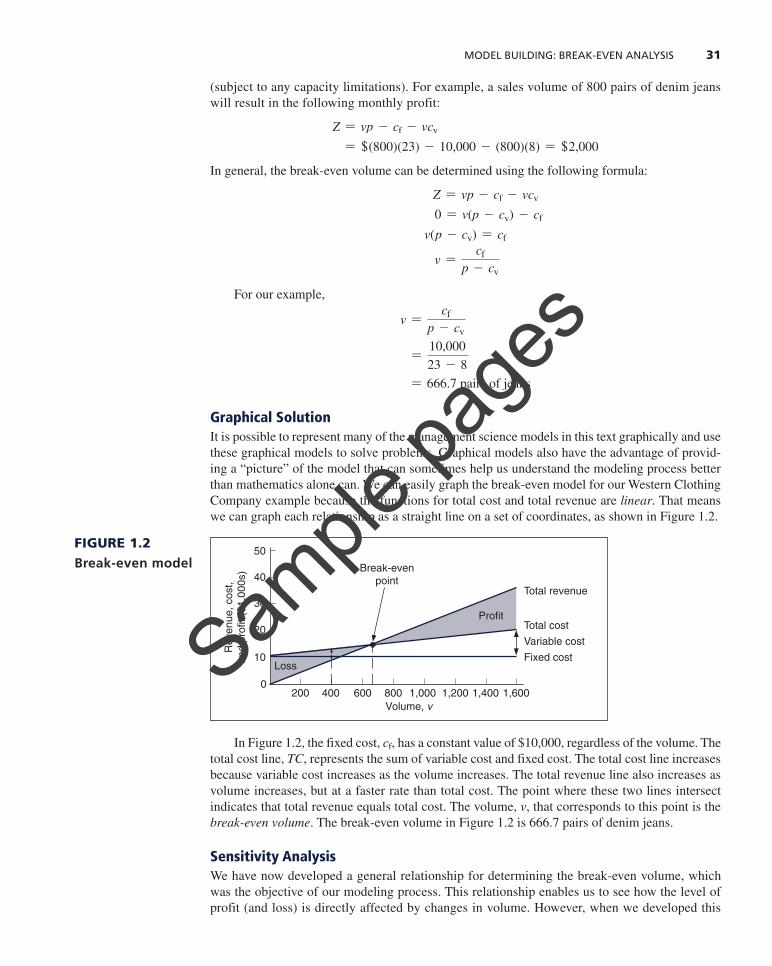
Graphical SolutionIt is possible to represent many of the management science models in this text graphically and use these graphical models to solve problems. Graphical models also have the advantage of provid-ing a “picture” of the model that can sometimes help us understand the modeling process better than mathematics alone can. We can easily graph the break-even model for our Western Clothing Company example because the functions for total cost and total revenue are linear. That means we can graph each relationship as a straight line on a set of coordinates, as shown in Figure 1.2.

FIGURE 1.2Break-even model

10

20

30

40

50

2000

400 600 800 1,000 1,200 1,400 1,600Volume, v

Total cost

Rev

enue

, cos

t, an

d pr

ofit (

$1,0

00s)

Variable cost

Fixed cost

Total revenue

Loss

Profit

Break-evenpoint

In Figure 1.2, the fixed cost, cf, has a constant value of $10,000, regardless of the volume. The total cost line, TC, represents the sum of variable cost and fixed cost. The total cost line increases because variable cost increases as the volume increases. The total revenue line also increases as volume increases, but at a faster rate than total cost. The point where these two lines intersect indicates that total revenue equals total cost. The volume, v, that corresponds to this point is the break-even volume. The break-even volume in Figure 1.2 is 666.7 pairs of denim jeans.

Sensitivity AnalysisWe have now developed a general relationship for determining the break-even volume, which was the objective of our modeling process. This relationship enables us to see how the level of profit (and loss) is directly affected by changes in volume. However, when we developed this

M01_TAYL3045_13_GE_C01.indd 31 26/10/2018 09:41

Sample

page

s

32 Chapter 1 ManageMent SCienCe

model, we assumed that our parameters, fixed and variable costs and price, were constant. In reality such parameters are frequently uncertain and can rarely be assumed to be constant, and changes in any of the parameters can affect the model solution. The study of changes on a man-agement science model is called sensitivity analysis—that is, seeing how sensitive the model is to changes.

Sensitivity analysis can be performed on all management science models in one form or another. In fact, sometimes companies develop models for the primary purpose of experimenta-tion to see how the model will react to different changes the company is contemplating or that management might expect to occur in the future. As a demonstration of how sensitivity analysis works, we will look at the effects of some changes on our break-even model.

The first thing we will analyze is price. As an example, we will increase the price for denim jeans from $23 to $30. As expected, this increases the total revenue, and it therefore reduces the break-even point from 666.7 pairs of jeans to 454.5 pairs of jeans:

v =cf

p - cv

=10,00030 - 8

= 454.5 pairs of denim jeans

The effect of the price change on break-even volume is illustrated in Figure 1.3.

Sensitivity analysis sees how sensitive a

management model is to changes.

In general, an increase in price

lowers the break-even point, all other things

held constant.

FIGURE 1.3Break-even model with an increase in price

10

20

30

40

50

2000

400 600 800 1,000 1,200 1,400 1,600Volume, v

Total cost

Rev

enue

, cos

t, an

d pr

ofit (

$1,0

00s)

New total revenue

Fixed cost

Old total revenue

Old B-E point

New B-E point

Although a decision to increase price looks inviting from a strictly analytical point of view, it must be remembered that the lower break-even volume and higher profit are possible but not guaranteed. A higher price can make it more difficult to sell the product. Thus, a change in price often must be accompanied by corresponding increases in costs, such as those for advertising, packaging, and possibly production (to enhance quality). However, even such direct changes as these may have little effect on product demand because price is often sensitive to numerous fac-tors, such as the type of market, monopolistic elements, and product differentiation.

When we increased price, we mentioned the possibility of raising the quality of the product to offset a potential loss of sales due to the price increase. For example, suppose the stitching on the denim jeans is changed to make the jeans more attractive and stronger. This change results in an increase in variable costs of $4 per pair of jeans, thus raising the variable cost per unit, cv, to $12 per pair. This change (in conjunction with our previous price change to $30) results in a new break-even volume:

v =cf

p - cv

=10,000

30 - 12= 555.5 pairs of denim jeans

In general, an increase in variable

costs will increase the break-even point, all other things held

constant.

M01_TAYL3045_13_GE_C01.indd 32 26/10/2018 09:41

Sample

page

s

CoMputer Solution 33

This new break-even volume and the change in the total cost line that occurs as a result of the variable cost change are shown in Figure 1.4.

FIGURE 1.4Break-even model with an increase in variable cost

10

20

30

40

50

2000

400 600 800 1,000 1,200 1,400 1,600Volume, v

Old total costR

even

ue, c

ost,

and

profi

t ($1

,000

s)

Total revenue

Fixed cost

New total cost

New B-E point

Old B-E point

FIGURE 1.5Break-even model with a change in fixed cost

10

20

30

40

50

2000

400 600 800 1,000 1,200 1,400 1,600Volume, v

Old total cost

Rev

enue

, cos

t, an

d pr

ofit (

$1,0

00s)

Total revenue

Old fixed cost

New total cost

New fixed cost

New B-E point

Old B-E point

Next let’s consider an increase in advertising expenditures to offset the potential loss in sales resulting from a price increase. An increase in advertising expenditures is an addition to fixed costs. For example, if the clothing company increases its monthly advertising budget by $3,000, then the total fixed cost, cf, becomes $13,000. Using this fixed cost, as well as the increased vari-able cost per unit of $12 and the increased price of $30, we compute the break-even volume as follows:

v =cf

p - cv

=13,000

30 - 12 = 722.2 pairs of denim jeans

This new break-even volume, representing changes in price, fixed costs, and variable costs, is illustrated in Figure 1.5. Notice that the break-even volume is now higher than the original volume of 666.7 pairs of jeans, as a result of the increased costs necessary to offset the potential loss in sales. This indicates the necessity to analyze the effect of a change in one of the break-even com-ponents on the whole break-even model. In other words, generally it is not sufficient to consider a change in one model component without considering the overall effect.

In general, an increase in fixed

costs will increase the break-even point, all other things held

constant.

Computer SolutionThroughout the text, we will demonstrate how to solve management science models on the com-puter by using Excel spreadsheets and QM for Windows, a general-purpose quantitative methods software package by Howard Weiss. QM for Windows has program modules to solve almost every

M01_TAYL3045_13_GE_C01.indd 33 26/10/2018 09:41

Sample

page

s

34 Chapter 1 ManageMent SCienCe

type of management science problem you will encounter in this text. There are a number of similar quantitative methods software packages available on the market, with characteristics and capabili-ties similar to those of QM for Windows. In most cases, you simply input problem data (i.e., model parameters) into a model template, click on a solve button, and the solution appears in a Windows format. QM for Windows is included on the companion Web site for this text.

Spreadsheets are not always easy to use, and you cannot conveniently solve every type of man-agement science model by using a spreadsheet. Most of the time, you must not only input the model parameters but also set up the model mathematics, including formulas, as well as your own model template with headings to display your solution output. However, spreadsheets provide a powerful reporting tool in which you can present your model and results in any format you choose. Spread-sheets such as Excel have become almost universally available to anyone who owns a computer. In addition, spreadsheets have become very popular as a teaching tool because they tend to guide the student through a modeling procedure, and they can be interesting and fun to use. However, because spreadsheets are somewhat more difficult to set up and apply than is QM for Windows, we will spend more time explaining their use to solve various types of problems in this text.

One of the difficult aspects of using spreadsheets to solve management science problems is setting up a spreadsheet with some of the more complex models and formulas. For the most com-plex models in the text, we will show how to use Excel QM, a supplemental spreadsheet macro that is included on the companion Web site for this text. A macro is a template or an overlay that already has the model format with the necessary formulas set up on the spreadsheet so that the user only has to input the model parameters.We will demonstrate Excel QM in six chapters, including this chapter, Chapter 6 (“Transportation, Transshipment, and Assignment Problems”), Chapter 12 (“Decision Analysis”), Chapter 13 (“Queuing Analysis”), Chapter 15 (“Forecasting”), and Chapter 16 (“Inventory Management”).

Later in this text, we will also demonstrate two spreadsheet add-ins, TreePlan and Crystal Ball. TreePlan is a program for setting up and solving decision trees that we use in Chapter 12 (“Decision Analysis”), whereas Crystal Ball is a simulation package that we use in Chapter 14 (“Simulation”). Also, in Chapter 8 (“Project Management”), we will demonstrate Microsoft Project.

In this section, we will demonstrate how to use Excel, Excel QM, and QM for Windows, using our break-even model example for Western Clothing Company.

Excel SpreadsheetsTo solve the break-even model using Excel, you must set up a spreadsheet with headings to iden-tify your model parameters and variables and then input the appropriate mathematical formulas into the cells where you want to display your solution. Exhibit 1.1 (which can be downloaded from the text website) shows the spreadsheet for the Western Clothing Company example. Setting up the different headings to describe the parameters and the solution is not difficult, but it does require that you know your way around Excel a little. Appendix B provides a brief tutorial titled “Setting Up and Editing a Spreadsheet” for solving management science problems.

EXHIBIT 1.1

Formula for v, break-evenpoint, =D4/(D8–D6)

M01_TAYL3045_13_GE_C01.indd 34 26/10/2018 09:41

Sample

page

s

CoMputer Solution 35

Notice that cell D10 contains the break-even formula, which is displayed on the toolbar near the top of the screen. The fixed cost of $10,000 is typed in cell D4, the variable cost of $8 is in cell D6, and the price of $23 is in cell D8.

As we present more complex models and problems in the chapters to come, the spreadsheets we develop to solve these problems will become more involved and will enable us to demonstrate different features of Excel and spreadsheet modeling.

The Excel QM Macro for SpreadsheetsExcel QM is included on the companion Web site for this text. You can install Excel QM onto your computer by following a brief series of steps displayed when the program is first accessed.

After Excel is started, Excel QM is normally accessed from the computer’s program files, where it is usually loaded. When Excel QM is activated, “Add-Ins” will appear at the top of the spreadsheet (as indicated in Exhibit 1.2). Clicking on “Excel QM” or “Taylor” will pull down a menu of the topics in Excel QM, one of which is break-even analysis. Clicking on “Break-Even Analysis” will result in the window for spreadsheet initialization. Every Excel QM macro listed on the menu will start with a Spreadsheet Initialization window.

EXHIBIT 1.2

Enter model parametersin cells B10:B12.

Click on “Excel QM,” then on“Alphabetical” list of modelsand select “Breakeven Analysis”

In this window, you can enter a spreadsheet title and choose under “Options” whether you also want volume analysis and a graph. Clicking on “OK” will result in the spreadsheet shown in Exhibit 1.2. The first step is to input the values for the Western Clothing Company example in cells B10 to B12, as shown in Exhibit 1.2. The spreadsheet shows the break-even volume in cell B17.

QM for WindowsYou begin using QM for Windows by clicking on the “Module” button on the toolbar at the top of the main window that appears when you start the program. This will pull down a window with

M01_TAYL3045_13_GE_C01.indd 35 26/10/2018 09:41

Sample

page

s

36 Chapter 1 ManageMent SCienCe

a list of all the model solution modules available in QM for Windows. Clicking on the “Break-even Analysis” module will access a new screen for typing in the problem title. Clicking again will access a screen with input cells for the model parameters—that is, fixed cost, variable cost, and price (or revenue). Next, clicking on the “Solve” button at the top of the screen will provide the solution and the break-even graph for the Western Clothing Company example, as shown in Exhibit 1.3.

Management Science Modeling TechniquesThis text focuses primarily on two of the five steps of the management science process described in Figure 1.1—model construction and solution. These are the two steps that use the manage-ment science techniques. In a textbook, it is difficult to show how an unstructured real-world problem is identified and defined because the problem must be written out. However, once a problem statement has been given, we can show how a model is constructed and a solution is derived. The techniques presented in this text can be loosely classified into four categories, as shown in Figure 1.6.

EXHIBIT 1.3

FIGURE 1.6Classification of management science techniques

Management science techniques

Probabilistictechniques

Linear mathematicalprogramming

Linear programming  modelsGraphical analysisSensitivity analysisTransportation,   transshipment, and assignmentInteger linear  programmingGoal programming

Decision analysis

Probability andstatistics

Queuing

Network

Text

techniques

Network flowProject

management(CPM/PERT)

Other techniques

ForecastingSimulation

Inventory

Analytical hierarchy  process (AHP)Nonlinear programming

Companion Web site

Branch and boundMarkov analysisGame theory

method

Simplex methodTransportation

and assignmentmethods

Nonlinear programming

Linear Mathematical Programming TechniquesChapters 2 through 6 and 9 present techniques that together make up linear mathematical program-ming. (The first example used to demonstrate model construction earlier in this chapter is a very rudimentary linear programming model.) The term programming used to identify this technique

M01_TAYL3045_13_GE_C01.indd 36 26/10/2018 09:41

Sample

page

s

ManageMent SCienCe Modeling teChniqueS 37

Management Science ApplicationManagement Science and Analytics

in major league baseball, popularized by the book and movie Moneyball. It was originally defined in 1980 by Bill James (cur-rently an analyst with the Boston Red Sox) as the “search for objective knowledge about baseball,” and it is derived from the acronym SABR (e.g., Society for American Baseball Research). It has generally evolved into the application of statistical analysis of baseball records to develop predictive models and measures to evaluate and compare the in-game performance of individual players, usually in terms of runs or team wins. Sabermetrics attempts to answer questions such as, which players on a team will contribute most to the team’s offense? For example, the sabermetric measure, VORP (value over replacement player), attempts to predict how much a hitter contributes offensively to his team in comparison to a fictitious average replacement player. A player might be worth 50 more runs in a season than a replacement level player at the same position (acquired at minimal cost). Currently every major league team has some employees in administrative positions dedicated to quantitative analytics for the evaluation of player performance to determine player acquisitions, trades, and contracts.

Sources: J. Byrum, C. Davis, G. Doonan, T. Doubler, D. Foster, B. Luzzi, R. Mowers, C. Zinselmeir, J. Klober, D. Culhane, and S. Mack, “Advanced Analytics for Agricultural Product Development,” Interfaces 46, no. 1 (January–February 2016): 5–17; S. Venkatachalam, F. Wong, E. Uyar, S. Ward, and A. Aggarwal, “Media Company Uses Analytics to Schedule Radio Advertisement Spots,” Interfaces 45, no. 6 (November–December 2015): 485–500; T. Fabusuyi, R. Hampshire, V. Hill, and K. Sasanuma, “Decision Analytics for Parking Availability in Downtown Pittsburgh,” Interfaces 44, no. 3 (May–June 2014): 286–299.

as we discussed in the section “Management Science and Business Analytics,” when applied to business prob-lems, analytics often combines the management science

approach to problem solving and decision making, including model building, with the use of data. Following are a few exam-ples of the many recent applications of analytics for problem solving in agriculture, media, urban planning, and sports.

Although the total world population is expected to grow by one-third to 9.6 billion in 2050, there will be less natural resources and land to support the necessary food production to feed an additional 2.4 billion people. Plant seed developer Syngenta is using analytics and management science models in its research and development efforts to develop and imple-ment a plant-breeding strategy for soybeans that will improve the quality and quantity of the soybeans that farmers produce per acre. Their application of analytics enables better decisions that result in reducing the time and cost required to develop higher-productivity crops, saving Syngenta an estimated $287 million in a five-year period, while making a contribution to meeting the world’s growing food needs.

iHeartMedia, Inc. (IHM) owns over 850 radio stations in more than 150 cities and provides programming (i.e., news, sports, traffic reports and weather) to over 2,250 stations. The company uses a set of management science models and sales data to maximize revenue from their inventory of radio adver-tising spots. Advertisers expect IHM to distribute their spots fairly and equitably across available inventory according to their order specifications, including dates, times, spot length, pro-grams, stations, and demographic targets. IHM uses two linear programming models to assign advertising spots. The use of analytics has resulted in a more efficient use of available inven-tory, improved customer service, and enhanced sales from more accurate inventory visibility, resulting in a financial benefit of over a half million dollars annually.

ParkPGH is a decision analytics application that provides real-time and predictive information for garage parking space availability within the downtown Pittsburgh Cultural District. The model collects real time parking information for garage gate counts and uses historical data and event schedules to predict parking availability and provide downtown visitors with information on available parking via mobile devices and the Internet. The system has reduced parking space search times and changed the perception of downtown patrons about the downtown parking situation (including security and availabil-ity), and also helped garage operators better manage park-ing demand. In one year the parking application received over 300,000 inquiries.

One of the most visible applications of analytics in the sports industry has been the development and use of “sabermetrics”

San Gabriel Valley Tribune/ZUMA Press Inc./Alamy Stock Photo

M01_TAYL3045_13_GE_C01.indd 37 26/10/2018 09:41

Sample

page

s

38 Chapter 1 ManageMent SCienCe

does not refer to computer programming but rather to a predetermined set of mathematical steps used to solve a problem. This particular class of techniques holds a predominant position in this text because it includes some of the more frequently used and popular techniques in management science.

In general, linear programming models help managers determine solutions (i.e., make deci-sions) for problems that will achieve some objective in which there are restrictions, such as limited resources or a recipe or perhaps production guidelines. For example, you could actually develop a linear programming model to help determine a breakfast menu for yourself that would meet dietary guidelines you may have set, such as number of calories, fat content, and vitamin level, while minimizing the cost of the breakfast. Manufacturing companies develop linear programming models to help decide how many units of different products they should produce to maximize their profit (or minimize their cost), given scarce resources such as capital, labor, and facilities.

Six chapters in this text are devoted to this topic because there are several variations of lin-ear programming models that can be applied to specific types of problems. Chapter 4 is devoted entirely to describing example linear programming models for several different types of problem scenarios. Chapter 6, for example, focuses on one particular type of linear programming applica-tion for transportation, transshipment, and assignment problems. An example of a transportation problem is a manager trying to determine the lowest-cost routes to use to ship goods from several sources (such as plants or warehouses) to several destinations (such as retail stores), given that each source may have limited goods available and each destination may have limited demand for the goods. Also, Chapter 9 includes the topic of goal programming, which is a form of linear programming that addresses problems with more than one objective or goal.

As mentioned previously in this chapter, some of the more mathematical topics in the text are included as supplementary modules on the companion Web site for the text. Among the linear programming topics included on the companion Web site are modules on the simplex method, the transportation and assignment solution methods, and the branch and bound solution method for integer programming models. Also included on the companion Web site are modules on nonlinear programming, game theory, and Markov analysis.

Probabilistic TechniquesProbabilistic techniques are presented in Chapters 11 through 13. These techniques are distinguished from mathematical programming techniques in that the results are probabilistic. Mathematical pro-gramming techniques assume that all parameters in the models are known with certainty. Therefore, the solution results are assumed to be known with certainty, with no probability that other solutions might exist. A technique that assumes certainty in its solution is referred to as deterministic. In contrast, the results from a probabilistic technique do contain uncertainty, with some possibility that alternative solutions might exist. In the model solution presented earlier in this chapter, the result of the first example (x = 25 units to produce) is deterministic, whereas the result of the second exam-ple (estimating an average of 40 units sold each month) is probabilistic.

An example of a probabilistic technique is decision analysis, the subject of Chapter 12. In deci-sion analysis, it is shown how to select among several different decision alternatives, given uncer-tain (i.e., probabilistic) future conditions. For example, a developer may want to decide whether to build a shopping mall, build an office complex, build condominiums, or not build anything at all, given future economic conditions that might be good, fair, or poor, each with a probability of occur-rence. Chapter 13, on queuing analysis, presents probabilistic techniques for analyzing waiting lines that might occur, for example, at the grocery store, at a bank, or at a movie. The results of waiting line analysis are statistical averages showing, among other things, the average number of customers in line waiting to be served or the average time a customer might have to wait for service.

Network TechniquesNetworks, the topic of Chapters 7 and 8, consist of models that are represented as diagrams rather than as strictly mathematical relationships. As such, these models offer a pictorial representation of the system under analysis. These models represent either probabilistic or deterministic systems.

A deterministic technique assumes

certainty in the solution.

M01_TAYL3045_13_GE_C01.indd 38 26/10/2018 09:41

Sample

page

s

buSineSS uSage of ManageMent SCienCe teChniqueS 39

For example, in shortest-route problems, one of the topics in Chapter 7 (“Network Flow Models”), a network diagram can be drawn to help a manager determine the shortest route among a number of different routes from a source to a destination. For example, you could use this tech-nique to determine the shortest or quickest car route from St. Louis to Daytona Beach for a spring break vacation. In Chapter 8 (“Project Management”), a network is drawn that shows the relation-ships of all the tasks and activities for a project, such as building a house or developing a new computer system. This type of network can help a manager plan the best way to accomplish each of the tasks in the project so that it will take the shortest amount of time possible. You could use this type of technique to plan for a concert or an intramural volleyball tournament on your campus.

Other TechniquesSome topics in the text are not easily categorized; they may overlap several categories, or they may be unique. The analytical hierarchy process (AHP) in Chapter 9 is such a topic that is not easily classified. It is a mathematical technique for helping the decision maker choose between several alternative decisions, given more than one objective; however, it is not a form of linear program-ming, as is goal programming, the shared topic in Chapter 9 (“Multicriteria Decision Making”). The structure of the mathematical models for nonlinear programming problems in Chapter 10 is similar to the linear programming problems in Chapters 2 through 6; however, the mathematical equations and functions in nonlinear programming can be nonlinear instead of linear, thus requir-ing the use of calculus to solve them. Simulation, the subject of Chapter 14, is probably the single most unique topic in the text. It has the capability to solve probabilistic and deterministic problems and is often the technique of last resort when no other management science technique will work. In simulation, a mathematical model is constructed (typically using a computer) that replicates a real-world system under analysis, and then that simulation model is used to solve problems in the “simulated” real-world system. For example, with simulation you could build a model to simulate the traffic patterns of vehicles at a busy intersection to determine how to set the traffic light signals.

Forecasting, the subject of Chapter 15, and inventory management, in Chapter 16, are top-ics traditionally considered to be part of the field of operations management. However, because they are both important business functions that also rely heavily on quantitative models for their analysis, they are typically considered important topics in the study of management science as well. Both topics also include probabilistic as well as deterministic aspects. In Chapter 15, we will look at several different quantitative models that help managers predict what the future demand for products and services will look like. In general, historical sales and demand data are used to build a mathematical function or formula that can be used to estimate product demand in the future. In Chapter 16, we will look at several different quantitative models that help organizations determine how much inventory to keep on hand to minimize inventory costs, which can be significant.

Business Usage of Management Science TechniquesNot all management science techniques are equally useful or equally used by business firms and other organizations. Some techniques are used quite frequently by business practitioners and managers; others are used less often. The most frequently used techniques are linear and integer programming, simulation, network analysis (including critical path method/project evaluation and review technique [CPM/PERT]), inventory control, decision analysis, and queuing theory, as well as probability and statistics. An attempt has been made in this text to provide a comprehensive treatment of all the topics generally considered within the field of management science, regardless of how frequently they are used. Although some topics may have limited direct applicability, their study can reveal informative and unique means of approaching a problem and can often enhance one’s understanding of the decision-making process.

The variety and breadth of management science applications and of the potential for apply-ing management science, not only in business and industry but also in government, health care, and service organizations, are extensive. Areas of application include project planning, capital

M01_TAYL3045_13_GE_C01.indd 39 26/10/2018 09:41

Sample

page

s

40 Chapter 1 ManageMent SCienCe

Management Science ApplicationManagement Science in Health Care

appointment times were overbooked by only 7.3 percent with few patients overscheduled and an estimated cost savings of about $95,000.

At the University of Tennessee Medical Center in Knox-ville, management science (including integer programming) was used to schedule a nine-physician group that provides 24-7 coverage for the 63-bed Neonatal Intensive Care Unit. Assigning physicians to shifts is problematic because of myr-iad constraints, including work rules and patterns based on quality-of-care and safety issues, workload and lifestyle choices, plus workload fairness that all members of the group consider equal in terms of apportioned work and times. The modeling approach created schedules that were individually preferred over acceptable equality schedules.

Sources: B. G. Thomas, S. Bollapragada, K. Akbay, D. Toledano, P. Katlic, O. Dulgeroglu, and D. Yang, “Automated Bed Assignments in a Complex Dynamic Hospital Environment,” Interfaces 43, no. 5 (September–October 2013): 435–448; J. C. Woodall, T. Gosselin, A. Boswell, M. Murr and B. T. Denton, “Improving Patient Access to Chemotherapy Treatment at Duke Cancer Center,” Interfaces 43, no. 5 (September–October 2013): 449–461; E. Lee, H. Atallah, M. Wright, E. Post, C. Thomas, D. Wu, and L. Haley, “Transforming Hospital Emergency Department Workflow and Patient Care,” Interfaces 45, no. 1 (January–February 2015): 58–82; J. Kros, S. Dellana, and D. West, “Overbooking Increases Patient Access at East Carolina University’s Student Health Services Clinic,” Interfaces 39, no. 3 (May–June 2009): 271–287; and M. Bowers, C. Noon, W. Wu, and J. Bass, “Neonatal Physician Scheduling at the University of Tennessee Medical Center,” Interfaces 46, no. 2 (March–April 2016): 168–182.

over 17 percent of the U.S. GDP is spent on health care each year (over $3 trillion), making it the single largest industry in the United States. However, it is estimated

that as much as 30 percent of health care costs result from waste through inefficient processes. Management science is really good at making inefficient processes more efficient. Thus, it is not surprising that one of the most frequent areas of application of management science techniques is in health care. Following are several brief examples of its many successful applications.

Improving patient flow through the hospital is a critical factor in improving hospital operating efficiency and reducing costs, and optimizing bed assignments is critical for patient flow. It is estimated that an average 300-bed hospital could add $10 million to its contribution margin with a 27 percent increase in bed utilization. At Mount Sinai Medical Center in New York a bed-assignment solution approach using a combi-nation of integer programming (Chapter 5) and goal program-ming (Chapter 9) reduced the average time from bed requests to bed assignments by 23 percent (from almost 4 hours to 3 hours). At the Duke Cancer Center a simulation model (Chap-ter 14) was used to predict patient waiting times and resource utilization in various departments throughout the hospital, including the outpatient clinic, radiology, and the oncology treatment center. This model identified nurse unavailability during oncology treatment as creating a serious bottleneck in patient flow. An integer programming model (Chapter 5) was used to develop optimal weekly and monthly nurse schedules that relieved the bottleneck. At Grady Memorial Hospital in Atlanta, the emergency department (ED) receives more than 125,000 patient visits per year. Using an analytics approach, including management science modeling (i.e., integer program-ming and simulation), the hospital was able to reduce patient length of stay by 33 percent to approximately 7 hours, reduce readmissions by 28 percent, reduce patient waiting times, and improved efficiencies in the ED reduced patient throughput by over 16 percent, resulting in annual revenues plus savings of $190 million, without additional funds or resources.

The East Carolina University (ECU) Student Health Service is a clinic that serves the 23,000 student body at this public university located in Greenville, South Carolina. In a one-year period, slightly over 35,000 appointments were scheduled with approximately 3,800 no-shows. The problem of no-shows at health care clinics is a significant problem, with estimated costs at the ECU clinic of over $400,000 per year (resulting from reduced patient access). Researchers at East Carolina used a combination of several management science techniques, includ-ing forecasting (Chapter 15), decision analysis (Chapter 12), and simulation (Chapter 14) to develop a solution approach employing an overbooking policy (similar to what airlines do for flights). In the first semester the clinic implemented the policy,

MShieldsPhotos/Alamy Stock Photo

M01_TAYL3045_13_GE_C01.indd 40 26/10/2018 09:41

Sample

page

s