Introduction to Magnetic Resonance Imaging Bruno Quesson, CR1 CNRS.
41
Introduction to Magnetic Resonance Imaging Bruno Quesson, CR1 CNRS
-
Upload
nicholas-lynch -
Category
Documents
-
view
225 -
download
1
Transcript of Introduction to Magnetic Resonance Imaging Bruno Quesson, CR1 CNRS.

Introduction to Magnetic Resonance Imaging
Bruno Quesson, CR1 CNRS

Important magnetic field (~1 Tesla)
General ElectricSiemensPhilips

MRI : Imaging of water and fat (soft tissues)

diagnostis
healthy pathological
brain
animal
breast
Fat suppression

Tunable contrasts

Multislices 2D / 3D
Any slice orientation is feasible
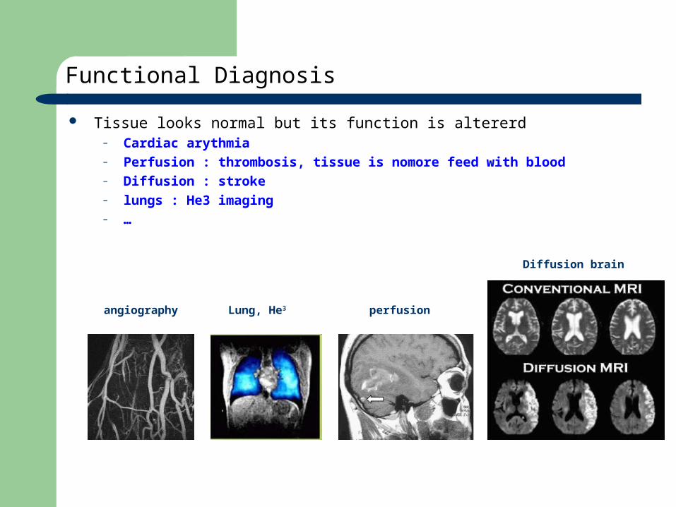
Functional Diagnosis
Tissue looks normal but its function is altererd– Cardiac arythmia – Perfusion : thrombosis, tissue is nomore feed with blood– Diffusion : stroke– lungs : He3 imaging– …
angiography perfusionLung, He3
Diffusion brain

Dynamic imaging (heart)

Spatial resolution can be adjusted
Embryo of mice

fMRI : functional imaging of the brain activity
signal changes with blood oxygenation– Task => use of oxygen– Indirect detection of the brain activity– Low signal variation (2%) => high filed
Dynamic imaging (kinetic) 3D imaging (cover the entire brain) Statistical analysis Associate PET (radioactivity) et EEG (electrical activity)

Interventional imaging
Definition : « guide a therapeutic procedure with the help of images»– Rapid acquisition -> real time– Real time reconstruction– Real time processing
Examples :
-to visualize catheter positioning – Substitution Xray to MRI
-to identify a lesion and to guide the puncture– Ex : breast, liver, brain tumours

Interventionnal imaging : thermometry
Pig liver
Human
temperature Thermal Dose Follow up T2 Follow up T1

HOW IS THIS POSSIBLE???

Nuclear Magnetic Resonance : NMR
Magnetic equilibrium : B0 static and intense
Perturbation of the equilibrium : Excitation B1 (energy transferred to the system)
Back to initial equilibrium state : Relaxation (energy transferred from the system)
B0 = 0
z
B0 ≠ 0
MacroscopicMagnetization M0y
x
z
y
x
zM0
zM0
zM0
B1
zM0
zM0
Emitted signal=
NMR signal

Modeling the NMR signal
Vector mathematical formalism
z
M
B0
y
x
Mz
Mx
My
Mx(t)=?
My(t)=?
Mz(t)=?
Solution of the Bloch differential equations :
Mx(t) = Mt(0).exp(-t/T2).cos(0 t)
My(t) = Mt(0).exp(-t/T2).sin(0 t)
Mz(t) = M0 – (M0 – Mz(0)).exp(-t/T1)
Transverse magnetization
Longitudinal magnetization
0 = B0

transverse magnetization : exponential decay
Helicoïdal motion
y
Mt
B0 x100
80
60
40
20
0
Mt
1.00.80.60.40.20.0
Time / s
Rotation around B0 Amplitude : exponential decay
Mt(t) = Mt(0).exp(-t/T2).exp(0 t)
Detectable signal

Longitudinal magnetization
z
B0 x
Mz
100
80
60
40
20
03.02.52.01.51.00.50.0
Mz
Time / s
Mz(t) = M0 – (M0 – Mz(0)).exp(-t/T1)
y

Typical NMR parameters at 1.5 Tesla
8550500breast
7055870cardiac muscle
951001800vitrous humor
7060775spleen
6060650kidney
6070600pancreas
7045500liver
8075934disk
951001200blood
4080830lung
10080252fat
4060400bone marrow
4060400Vertebral marrow
7045870SQuel Muscle
1001602400CSF
7090780WM
85100920GM
M0 (%)T2 / msT1 / msTissue

Longitudinal (T1) and Transverse (T2) relaxation times
M0(GM)
M0(WM)
100
80
60
40
20
0
Mz
3.02.52.01.51.00.50.0
GM WM
100
80
60
40
20
0
Mt
1.00.80.60.40.20.0
GM WM
Time / s
Difference = contrast
T1 contrast
T2 contrast
Proton Density
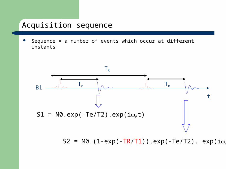
Acquisition sequence
Sequence = a number of events which occur at different instants
t
B1
TR
Te
S2 = M0.(1-exp(-TR/T1)).exp(-Te/T2). exp(i0t)
Te
S1 = M0.exp(-Te/T2).exp(i0t)

Which contrast ?
TR/T1
TE/T2
ContrastT1
ProtonDensity
ContrastT1 and T2
ContrastT2
0

Examples
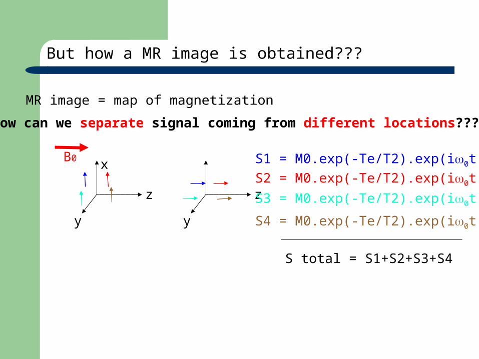
But how a MR image is obtained???
MR image = map of magnetization
How can we separate signal coming from different locations????
B0
y
x
z
y
z
S1 = M0.exp(-Te/T2).exp(i0t)
S2 = M0.exp(-Te/T2).exp(i0t)
S3 = M0.exp(-Te/T2).exp(i0t)
S4 = M0.exp(-Te/T2).exp(i0t)
S total = S1+S2+S3+S4

So what??
t
t
t
t
t
Fourier Transformation
It is NOT possible to distinguish individual signals
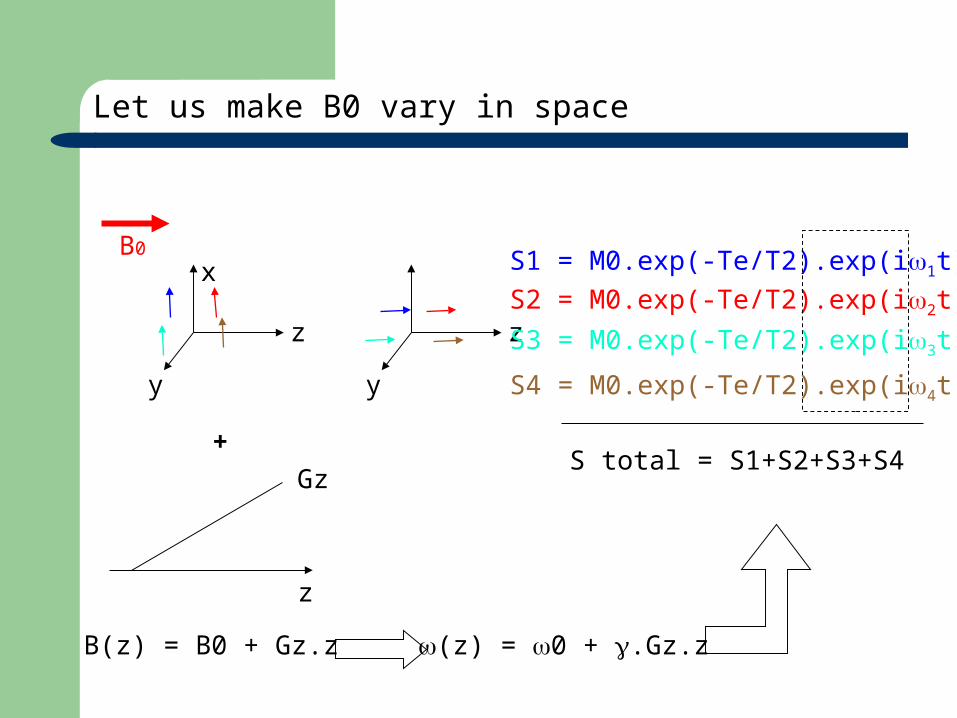
Let us make B0 vary in space
B0
y
x
z
y
z
S1 = M0.exp(-Te/T2).exp(i1t)
S2 = M0.exp(-Te/T2).exp(i2t)
S3 = M0.exp(-Te/T2).exp(i3t)
S4 = M0.exp(-Te/T2).exp(i4t)
S total = S1+S2+S3+S4
z
B(z) = B0 + Gz.z (z) = 0 + .Gz.z
+
Gz
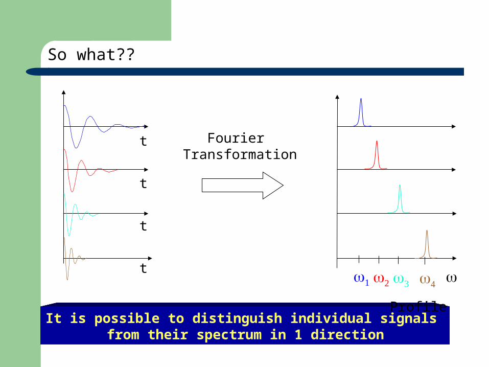
So what??
t
t
t
t
Fourier Transformation
It is possible to distinguish individual signals from their spectrum in 1 direction
Profile
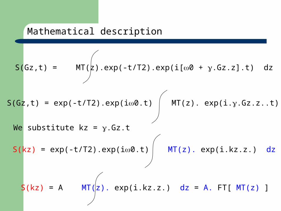
Mathematical description
S(Gz,t) = MT(z).exp(-t/T2).exp(i[0 + .Gz.z].t) dz
S(Gz,t) = exp(-t/T2).exp(i0.t) MT(z). exp(i..Gz.z..t) dz
S(kz) = exp(-t/T2).exp(i0.t) MT(z). exp(i.kz.z.) dz
We substitute kz = .Gz.t
S(kz) = A MT(z). exp(i.kz.z.) dz = A. FT[ MT(z) ]

Back to the profile
MT(z) = FT-1 [ S(kz) ] / A
MT(z) = A-1 . S(kz). exp(-i.kz.z.) dkz
1-We have to measure the signal for different kz (= g.Gz.t) conditions
2-We have to Fourier Transform these data sets to retrieve the profile of the object

Comparison of measurements under different Gz conditions
z
Gz
z
Gz
z
Gz
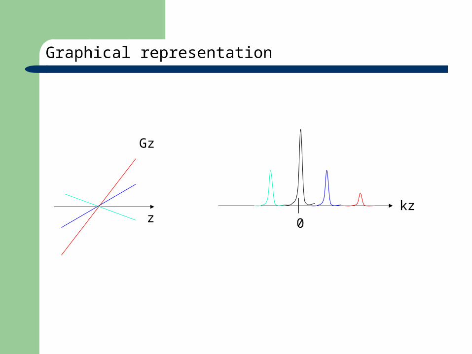
Graphical representation
zkz
Gz
0
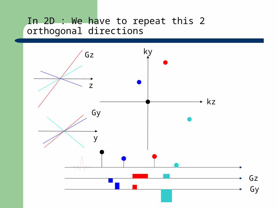
In 2D : We have to repeat this 2 orthogonal directions
z
kz
Gz
y
Gy
ky
Gz
Gy
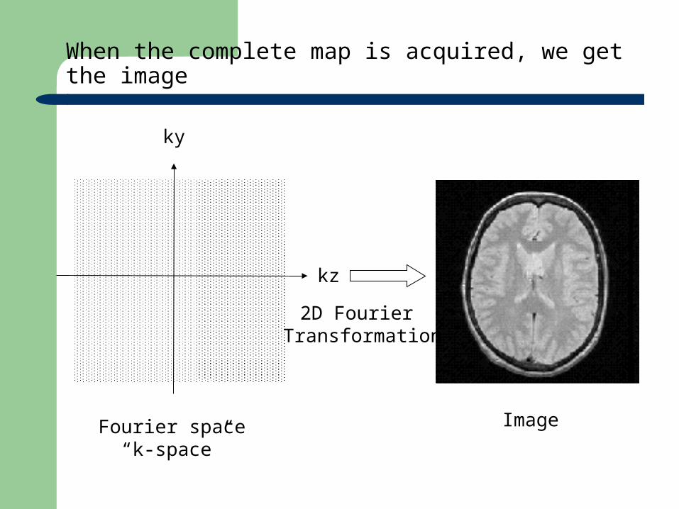
When the complete map is acquired, we get the image
kz
2D Fourier Transformation
ky
ImageFourier space“k-space”

MRI acquisition sequence
t
t
t
t
B1
Gs
Gp
Gr
TR
Te
Gradient echo
Trajectory in the Fourier space
Contrast

Contrast manipulation
PreparationAcquisition (of Fourier space)
t
t
t
t
B1
Gs
Gp
Gr
TeTi
t
Ex: inversion recovery (IR)

Examples of signal modulation with Inversion -Recovery
Ti = 0 s
Ti = 66 ms
Ti = 174 ms
MT(t) = MT(0).exp(-t/T2)
MT(0) = M0(1 – 2.exp(-Ti/T1))
Signal :
with :
Contrast modulation
-100
-50
0
50
100
Mz
1.21.00.80.60.40.20.0
Time / s
fat liver
100
80
60
40
20
0
Mt
0.40.30.20.10.0
fat liver
60
50
40
30
20
10
0
Mt
0.40.30.20.10.0
fat liver
100
80
60
40
20
0
Mt
0.40.30.20.10.0
Time / s
fat liver
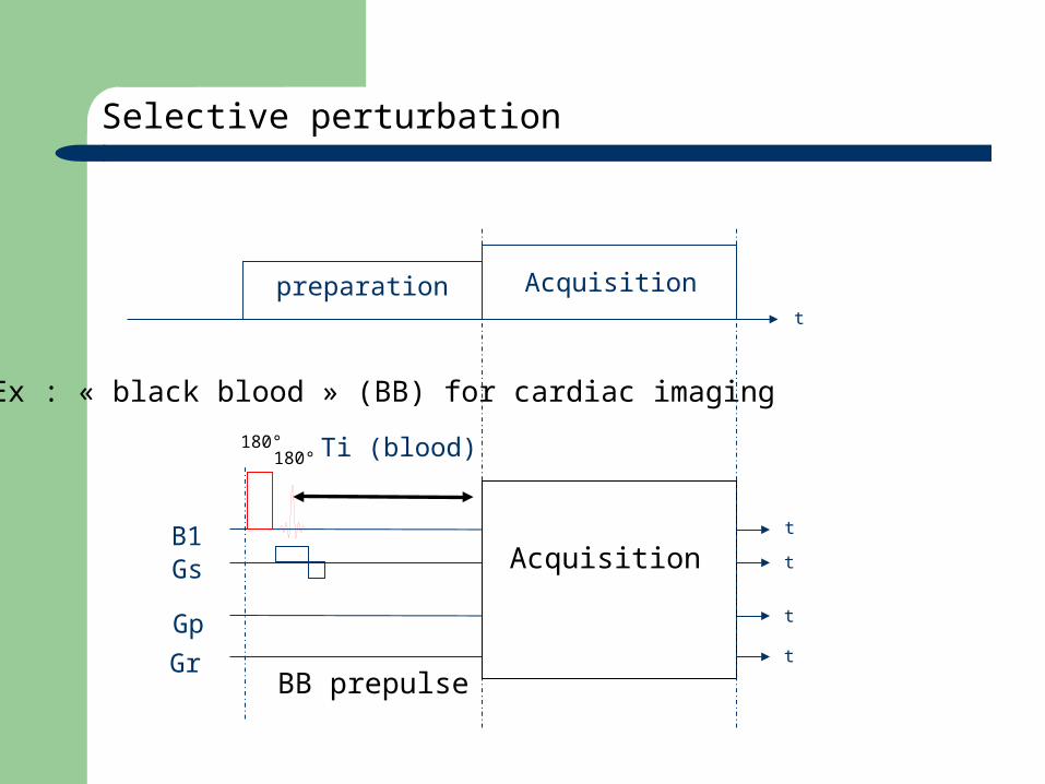
Selective perturbation
Ex : « black blood » (BB) for cardiac imaging
t
t
t
t
B1Gs
Gp
Gr
Ti (blood)
Acquisition
180°180°
BB prepulse
Acquisitionpreparationt

Resulting images
Without BB
With BB pulse

Double inversion-recovery
t
t
t
t
B1Gs
Gp
Gr
Acquisition
180°180°
Motif DI
Ti(1) Ti(2)

Gradient Echo sequence
t
t
t
t
B1
Gs
Gp
Gr
TR
Te
Gradient echo
Trajectory in the Fourier space
Contrast

Spin echo sequence
Refocuses all magnetizations
t
t
t
t
B1
Gs
Gp
Gr
TR
Te
Te/2Te/2
Spin echo
Summary
RF pulses– Variable angles– Frequency selective or not– Spatially selective or not
Gradients
A lot of possible combinaisons
Strategy of the acquisition depends on the application