
Introduction to LiveLink for MATLAB - UPB · 2012-04-27 · Introduction | 5 Introduction This...
48
VERSION 4.3 Introduction to LiveLink for MATLAB ® TM
Transcript of Introduction to LiveLink for MATLAB - UPB · 2012-04-27 · Introduction | 5 Introduction This...

VERSION 4.3
Introduction to LiveLink
for MATLAB®
TM

C o n t a c t I n f o r m a t i o n
Visit www.comsol.com/contact for a searchable list of all COMSOL offices and local representatives. From this web page, search the contacts and find a local sales representative, go to other COMSOL websites, request information and pricing, submit technical support queries, subscribe to the monthly eNews email newsletter, and much more.
If you need to contact Technical Support, an online request form is located at www.comsol.com/support/contact.
Other useful links include:
• Technical Support www.comsol.com/support
• Software updates: www.comsol.com/support/updates
• Online community: www.comsol.com/community
• Events, conferences, and training: www.comsol.com/events
• Tutorials: www.comsol.com/products/tutorials
• Knowledge Base: www.comsol.com/support/knowledgebase
Part No. CM020010
I n t r o d u c t i o n t o L i v e L i n k™ f o r M A T L A B® 2009–2012 COMSOL
Protected by U.S. Patents 7,519,518; 7,596,474; and 7,623,991. Patents pending.
This Documentation and the Programs described herein are furnished under the COMSOL Software License Agreement (www.comsol.com/sla) and may be used or copied only under the terms of the license agree-ment.
COMSOL, COMSOL Desktop, COMSOL Multiphysics, and LiveLink are registered trademarks or trade-marks of COMSOL AB. MATLAB is a registered trademark of The MathWorks, Inc.. Other product or brand names are trademarks or registered trademarks of their respective holders.
Version: May 2012 COMSOL 4.3
Contents
Introduction . . . . . . . . . . . . . . . . . . . . . . . . . . . . . . . . . . . .5
Starting COMSOL with MATLAB . . . . . . . . . . . . . . . . .6
A Thorough Example: The Busbar . . . . . . . . . . . . . . . . .8
Exchanging Models with the COMSOL Desktop . . . .23
Extracting Results at the MATLAB Command Line . .28
Automating with MATLAB Scripts . . . . . . . . . . . . . . . .32
Using External MATLAB Functions. . . . . . . . . . . . . . . .42
| 3

4 |

IntroductionThis guide introduces you to LiveLink™ for MATLAB®. The examples guide you through the process of setting-up a COMSOL model and explain how to use COMSOL Multiphysics within the MATLAB scripting environment.
Introduction | 5

Starting COMSOL with MATLAB
STARTING ON WINDOWS
To star t COMSOL Multiphysics with MATLAB double-click on the COMSOL with MATLAB icon available on the desktop.
This opens the MATLAB desktop together with the COMSOL server, which is represented by the command window appearing in the background.
STARTING ON MAC OS X
Navigate to Applications>COMSOL 4.3>COMSOL 4.3 with MATLAB.
An alternative way is to use a terminal window and enter the command:
comsol server matlab
STARTING ON LINUX
Start a terminal prompt and run the comsol command, which is located inside the bin folder in the COMSOL installation directory:
comsol server matlab
6 | Starting COMSOL with MATLAB

THE COMSOL CLIENT SERVER
The LiveLink interface is based on the COMSOL client/server architecture. A COMSOL thin client is running inside MATLAB and has access to the COMSOL API through the MATLAB Java interface. Model information is stored in a model object available on the COMSOL server. The thin client communicates with the COMSOL server, enabling you to generate, modify, and solve COMSOL model objects at the MATLAB prompt.
When star ting COMSOL with MATLAB, you open both the COMSOL server and the MATLAB desktop. The first time you are required to enter a username and password. Once this information is entered, the client/server communication is established. The information is stored in the user preferences, so that subsequent star ts do not require you to enter it again.
Both the COMSOL server and the MATLAB desktop are run on the same computer. For computations requiring more memory you can connect to a remote server, but this configuration requires a floating network license.
Note that the COMSOL Desktop is not used when running COMSOL Multiphysics with MATLAB. You can star t the COMSOL Desktop separately to import models available in the COMSOL server connected to MATLAB. See “Exchanging Models with the COMSOL Desktop” for more information.
Starting COMSOL with MATLAB | 7
A Thorough Example: The BusbarThis example familiarizes you with the COMSOL model object and the COMSOL API syntax. In this section, learn how to:
• Create a geometry
• Set up a mesh and apply physics properties
• Solve the problem
• Generate results for analysis
• Exchange the model between the scripting interface of MATLAB and the COMSOL desktop.
The model you are building at the MATLAB command line is the same model described in the Introduction to COMSOL Multiphysics. The difference is that in that guide it is set up using the COMSOL Desktop instead of the COMSOL model object.
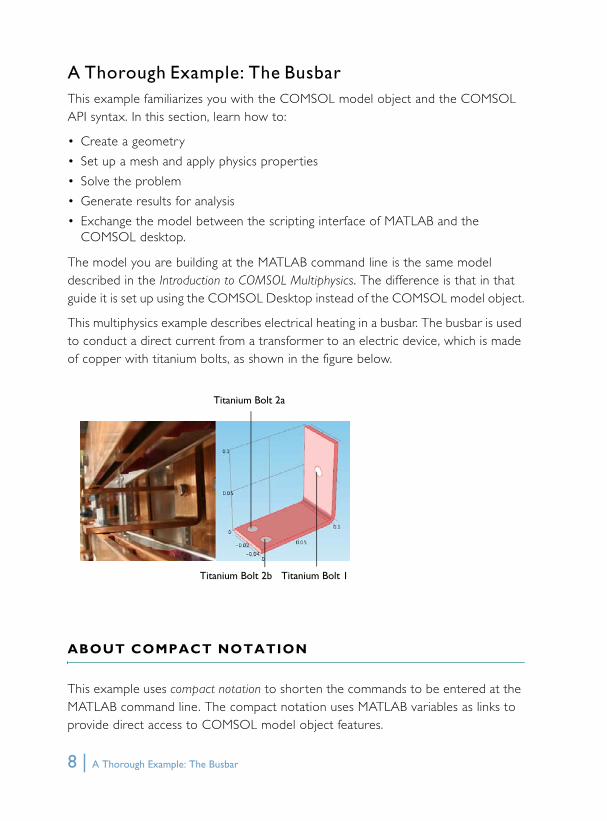
This multiphysics example describes electrical heating in a busbar. The busbar is used to conduct a direct current from a transformer to an electric device, which is made of copper with titanium bolts, as shown in the figure below.
ABOUT COMPACT NOTATION
This example uses compact notation to shorten the commands to be entered at the MATLAB command line. The compact notation uses MATLAB variables as links to provide direct access to COMSOL model object features.
Titanium Bolt 2a
Titanium Bolt 1Titanium Bolt 2b
8 | A Thorough Example: The Busbar

For example, to create a block using the compact notation, enter :
blk1 = geom1.feature.create('blk1', 'Block');blk1.setIndex('size', '2', 0);blk1.setIndex('size', '3', 1);
This creates a block, then changes its width to 2 and its depth to 3.
Compared to above, the commands using a full notation are:
geom1.feature.create('blk1', 'Block');geom1.feature('blk1').setIndex('size', '2', 0);geom1.feature('blk1').setIndex('size', '3', 1);
When a model object is saved in the M-file format the full notation is always used.
Note: 'blk1'(with quotes) is the block geometry tag defined inside the COMSOL model object. The variable blk1 (without quotes), defined only in MATLAB, is the link to the block feature. By linking MATLAB variables to features you can directly access and modify features of the COMSOL model object in an efficient manner.
ABOUT THE MODEL OBJECT
The model object contains all the information about a model, from the geometry to the results. The model object is defined on the COMSOL server and can be accessed at the MATLAB command line using a link in MATLAB.
1 Start COMSOL with MATLAB as in the section “Starting COMSOL with MATLAB”.
2 Start modeling by creating a model object on the COMSOL server :model = ModelUtil.create('Model');
The model object on the COMSOL server has the tag Model while the variable model is its link in MATLAB.
To access and modify the model object the LiveLink interface uses the COMSOL API syntax.
3 Set a name for the model object:model.name('busbar');
The name defined by the name method is intended only for visualization purposes when exporting the model to the COMSOL Desktop.
A Thorough Example: The Busbar | 9

ABOUT GLOBAL PARAMETERS
If you plan to solve your problem for several different parameter values, it is convenient to define them in the Parameters node, and to take advantage of the COMSOL parametric sweep functionality. Global parameters can be used in expressions during all stages of the model set-up, for example, when creating geometry, applying physics, or defining the mesh.
1 Define the parameters for the busbar model:model.param.set('L', '9[cm]', 'Length of the busbar');model.param.set('rad_1', '6[mm]', 'Radius of the fillet');model.param.set('tbb', '5[mm]', 'Thickness');model.param.set('wbb', '5[cm]', 'Width');model.param.set('mh', '6[mm]', 'Maximum element size');model.param.set('htc', '5[W/m^2/K]', 'Heat transfer coefficient');model.param.set('Vtot', '20[mV]', 'Applied electric potential');
GEOMETRY
1 Create a 3D geometry node:geom1 = model.geom.create('geom1', 3);
The create method of the geometry node requires as input a tag for the geometry name ('geom1'), and the geometry space dimension (3 for 3D).
2 The initial geometry is obtained by extruding a 2D drawing. Create a work plane tagged 'wp1', and set it as the xz-plane of the 3D geometry:wp1 = geom1.feature.create('wp1', 'WorkPlane');wp1.set('quickplane', 'xz');
3 In this work plane, create a rectangle and set the width to L+2*tbb and the height to 0.1:r1 = wp1.geom.feature.create('r1', 'Rectangle');r1.set('size', {'L+2*tbb' '0.1'});
Note: When the size properties of the rectangle are enclosed with single quotes ' ', it indicates that the variables L and tbb are defined within the model object. In this case they are defined in the Parameters node.
4 Create a second rectangle and set the width to L+tbb and the height to 0.1-tbb. Then change the rectangle position to (0;tbb):r2 = wp1.geom.feature.create('r2', 'Rectangle');r2.set('size', {'L+tbb' '0.1-tbb'});r2.set('pos', {'0' 'tbb'});
10 | A Thorough Example: The Busbar

5 Subtract rectangle r2 from rectangle r1, by creating a Difference feature with the 'input' property set to r1 and the 'input2' property set to r2:dif1 = wp1.geom.feature.create('dif1', 'Difference');dif1.selection('input').set({'r1'});dif1.selection('input2').set({'r2'});
Display the current geometry using mphgeom. Enter at the MATLAB prompt:
mphgeom(model,'geom1');
6 Round the inner corner by creating a Fillet feature and set point 3 in the selection property. Then set the radius to tbb:fil1 = wp1.geom.feature.create('fil1', 'Fillet');fil1.selection('point').set('dif1(1)', 3);fil1.set('radius', 'tbb');
7 Round the outer corner by creating a new Fillet feature, then select point 6 and set the radius to 2*tbb:fil2 = wp1.geom.feature.create('fil2', 'Fillet');fil2.selection('point').set('fil1(1)', 6);fil2.set('radius', '2*tbb');
For geometry operations the name of the resulting geometry objects is formed by appending a numeral in parenthesis to the tag of the geometry operation. Above, 'fil1(1)' is the result of the 'fil1' operation.
8 Extrude the geometry objects in the work plane. Create an Extrude feature, set the work plane wp1 as input and the distance to wbb:ext1 = geom1.feature.create('ext1', 'Extrude');ext1.selection('input').set({'wp1'});ext1.set('distance', {'wbb'});
A Thorough Example: The Busbar | 11

You can plot the current geometry by entering the following command at the MATLAB prompt:
mphgeom(model)
The busbar shape is now generated. Next create the cylinder that represent the bolts connecting the busbar to the external frame (not represented in the model).
9 Create a new work plane and set the planetype property to faceparallel. Then set the selection to boundary 8: wp2 = geom1.feature.create('wp2', 'WorkPlane');wp2.set('planetype', 'faceparallel');wp2.selection('face').set('ext1(1)', 8);
10Create a circle and set the radius to rad_1:c1 = wp2.geom.feature.create('c1', 'Circle');c1.set('r', 'rad_1');
11Create an Extrude node, select the second work plane wp2 as input, and then set the extrusion distance to -2*tbb:ext2 = geom1.feature.create('ext2', 'Extrude');ext2.selection('input').set({'wp2'});ext2.set('distance', {'-2*tbb'});
12Create a new workplane, set planetype to faceparallel, then set the selection to boundary 4:wp3 = geom1.feature.create('wp3', 'WorkPlane');wp3.set('planetype', 'faceparallel');wp3.selection('face').set('ext1(1)', 4);
13Create a circle, then set the radius to rad_1 and set the position of the center to (-L/2+1.5e-2;-wbb/4):
12 | A Thorough Example: The Busbar

c2 = wp3.geom.feature.create('c2', 'Circle');c2.set('r', 'rad_1');c2.set('pos', {'-L/2+1.5e-2' '-wbb/4'});
14Create a second circle in the work plane by copying the previous circle and displacing it a distance wbb/2 in the y-direction:copy1 = wp3.geom.feature.create('copy1', 'Copy');copy1.selection('input').set({'c2'});copy1.set('disply', 'wbb/2');
15Extrude the circles c2 and copy1 from the work plane wp3 a distance -2*tbb:ext3 = geom1.feature.create('ext3', 'Extrude');ext3.selection('input').set({'wp3.c2' 'wp3.copy1'});ext3.set('distance', {'-2*tbb'});
16Build the entire geometry sequence, including the finalize node using the run method:geom1.run;
Note: The run method only builds features which need re-building or have not yet been built, including the finalize node.
17Display the geometry with the mphgeom command:
mphgeom(model)
A Thorough Example: The Busbar | 13
SELECTIONS
You can create selections of geometric entities such as domains, boundaries, edges, or points. These selections can be accessed during the modeling process with the advantage of not having to select the same entities several times.
1 To create a domain selection corresponding to the titanium bolts, named Ti bolts enter:sel1 = model.selection.create('sel1');sel1.set([2 3 4 5 6 7]);sel1.name('Ti bolts');
MATERIAL PROPERTIES
The Material node of the model object stores the material properties. In this example the Joule Heating interface is used to involve both an electric current and a heat balance. Thus, the electrical conductivity, the heat capacity, the relative permittivity, the density, and the thermal conductivity of the materials all need to be defined.
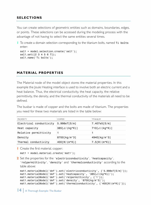
The busbar is made of copper and the bolts are made of titanium. The properties you need for these two materials are listed in the table below:
1 Create the first material, copper:mat1 = model.material.create('mat1');
2 Set the properties for the 'electricconductivity', 'heatcapacity', 'relpermittivity', 'density' and 'thermalconductivity' according to the table above:mat1.materialModel('def').set('electricconductivity', {'5.998e7[S/m]'});mat1.materialModel('def').set('heatcapacity', '385[J/(kg*K)]');mat1.materialModel('def').set('relpermittivity', {'1'});mat1.materialModel('def').set('density', '8700[kg/m^3]');mat1.materialModel('def').set('thermalconductivity', {'400[W/(m*K)]'});
PROPERTY COPPER TITANIUM
Electrical conductivity 5.998e7[S/m] 7.407e5[S/m]
Heat capacity 385[J/(kg*K)] 710[J/(kg*K)]
Relative permittivity 1 1
Density 8700[kg/m^3] 4940[kg/m^3]
Thermal conductivity 400[W/(m*K)] 7.5[W/(m*K)]
14 | A Thorough Example: The Busbar
3 Set the name of the material to 'Copper'. By default the first material is assigned to all domains:mat1.name('Copper');
4 Create a second material using the material properties for titanium, and set its name to 'Titanium' :mat2 = model.material.create('mat2');mat2.materialModel('def').set('electricconductivity', {'7.407e5[S/m]'});mat2.materialModel('def').set('heatcapacity', '710[J/(kg*K)]');mat2.materialModel('def').set('relpermittivity', {'1'});mat2.materialModel('def').set('density', '4940[kg/m^3]');mat2.materialModel('def').set('thermalconductivity', {'7.5[W/(m*K)]'});mat2.name('Titanium');
5 Assign the material to the selection 'sel1' (corresponding to the bolt domains) created previously:
mat2.selection.named('sel1');
Only one material per domain can be assigned. This means that the last operation automatically removes the bolts from the selection of the copper material.
PHYSICS INTERFACE
The Physics node contains the settings of the physics interfaces, including the domain and the boundary settings. Settings are grouped together according to the physics interface they belong to. To model the electrothermal interaction of this example, add the JouleHeating interface to the model. Apply a fixed electric potential to the upper bolt and ground the two lower bolts. In addition, assume that the device is cooled by convection, approximated by a heat flux with a defined heat transfer coefficient on all outer faces except where the bolts are connected.
1 Create the JouleHeating interface on the geom1 geometry:jh = model.physics.create('jh', 'JouleHeating', 'geom1');
2 Create a heat flux boundary condition and set the type to InwardHeatFlux:hf1 = jh.feature.create('hf1', 'HeatFluxBoundary', 2);
Note: The third argument of the create method, the space dimension sdim, indicates at which geometry level (domain, boundary, edge, or point) the feature should be applied to. In the above commands 'HeatFluxBoundary' feature applies to boundaries, which have the space dimension 2.
A Thorough Example: The Busbar | 15
3 Now apply the cooling to all exterior boundaries 1 to 43 except the bolt connection boundaries 8, 15, and 43. An InwardHeatFlux boundary condition requires a heat transfer coefficient. Set its value to the previously defined parameter htc:hf1.set('HeatFluxType', 'InwardHeatFlux');hf1.selection.set([1:7 9:14 16:42]);hf1.set('h', 'htc');
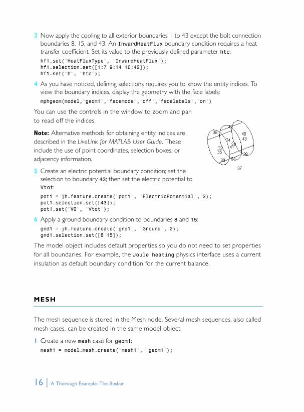
4 As you have noticed, defining selections requires you to know the entity indices. To view the boundary indices, display the geometry with the face labels:mphgeom(model,'geom1','facemode','off','facelabels','on')
You can use the controls in the window to zoom and pan to read off the indices.
Note: Alternative methods for obtaining entity indices are described in the LiveLink for MATLAB User Guide. These include the use of point coordinates, selection boxes, or adjacency information.
5 Create an electric potential boundary condition; set the selection to boundary 43; then set the electric potential to Vtot:pot1 = jh.feature.create('pot1', 'ElectricPotential', 2);pot1.selection.set([43]);pot1.set('V0', 'Vtot');
6 Apply a ground boundary condition to boundaries 8 and 15:gnd1 = jh.feature.create('gnd1', 'Ground', 2);gnd1.selection.set([8 15]);
The model object includes default proper ties so you do not need to set properties for all boundaries. For example, the Joule heating physics interface uses a current insulation as default boundary condition for the current balance.
MESH
The mesh sequence is stored in the Mesh node. Several mesh sequences, also called mesh cases, can be created in the same model object.
1 Create a new mesh case for geom1:mesh1 = model.mesh.create('mesh1', 'geom1');
16 | A Thorough Example: The Busbar

2 By default the mesh sequence contains at least a size feature, which applies to all the subsequent meshing operations. First create a link to the existing size feature and then set the maximum element size hmax to mh and the minimum element size hmin to mh-mh/3. Then set the curvature factor hcurve to 0.2:size = mesh1.feature('size');size.set('hmax', 'mh');size.set('hmin', 'mh-mh/3');size.set('hcurve', '0.2');
3 Create a free tetrahedron mesh:ftet1 = mesh1.feature.create('ftet1', 'FreeTet');
4 Build the mesh:mesh1.run;
5 Visualize the mesh in a MATLAB figure using the command mphmesh:mphmesh(model)
STUDY
In order to solve the model you need to create a Study node where the analysis type is set to be solved for.
1 Create a study node and add a stationary study step:std1 = model.study.create('std1');stat = std1.feature.create('stat', 'Stationary');
2 By default the progress bar for the solve and mesh operations is not displayed. To activate the progress bar enter:ModelUtil.showProgress(true)
Once activated, the progress bar is displayed in a separate window during mesh or solver operations. The Progress window also contains log information.
Note: The progress bar is not available on MAC OS X.
A Thorough Example: The Busbar | 17
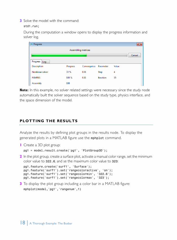
3 Solve the model with the command:std1.run;
During the computation a window opens to display the progress information and solver log.
Note: In this example, no solver related settings were necessary since the study node automatically built the solver sequence based on the study type, physics interface, and the space dimension of the model.
PLOTTING THE RESULTS
Analyze the results by defining plot groups in the results node. To display the generated plots in a MATLAB figure use the mphplot command.
1 Create a 3D plot group:pg1 = model.result.create('pg1', 'PlotGroup3D');
2 In the plot group, create a surface plot, activate a manual color range, set the minimum color value to 322.6, and se the maximum color value to 323:pg1.feature.create('surf1', 'Surface');pg1.feature('surf1').set('rangecoloractive', 'on');pg1.feature('surf1').set('rangecolormin', '322.6');pg1.feature('surf1').set('rangecolormax', '323');
3 To display the plot group including a color bar in a MATLAB figure:mphplot(model,'pg1','rangenum',1)
18 | A Thorough Example: The Busbar

If several plot types are available in the same plot group, you can define which color bar to display. The value of the rangenum property corresponds to the plot type number in the plot group sequence.
4 Create a second plot group, with a surface plot type, and plot the norm of the current density. Set the maximum color range value to 1e6. Finally, add the title 'Current density norm (A/m^2)', display the plot in a MATLAB figure:
pg2 = model.result.create('pg2', 'PlotGroup3D');pg2.feature.create('surf1', 'Surface');pg2.feature('surf1').set('expr', 'jh.normJ');pg2.feature('surf1').set('rangecoloractive', 'on');pg2.feature('surf1').set('rangecolormax', '1e6');pg2.set('title', 'Current density norm (A/m^2)');mphplot(model,'pg2','rangenum',1);
A Thorough Example: The Busbar | 19
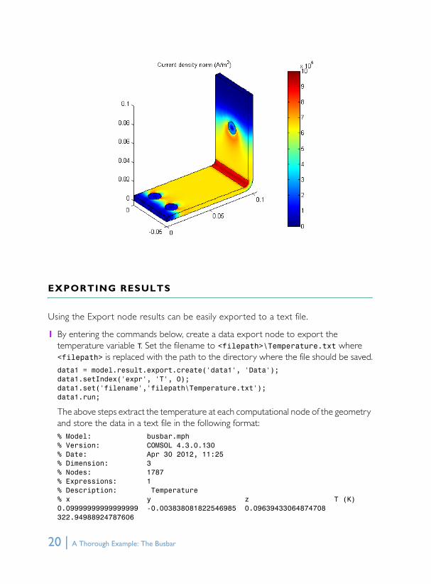
EXPORTING RESULTS
Using the Export node results can be easily exported to a text file.
1 By entering the commands below, create a data export node to export the temperature variable T. Set the filename to <filepath>\Temperature.txt where <filepath> is replaced with the path to the directory where the file should be saved.data1 = model.result.export.create('data1', 'Data');data1.setIndex('expr', 'T', 0);data1.set('filename','filepath\Temperature.txt');data1.run;
The above steps extract the temperature at each computational node of the geometry and store the data in a text file in the following format:% Model: busbar.mph% Version: COMSOL 4.3.0.130% Date: Apr 30 2012, 11:25% Dimension: 3% Nodes: 1787% Expressions: 1% Description: Temperature% x y z T (K)0.09999999999999999 -0.003838081822546985 0.09639433064874708 322.94988924787606
20 | A Thorough Example: The Busbar

0.09749606929798824 -0.006999750297542365 0.1 322.949261374022460.09999999999999996 -0.005555555555555556 0.1 322.94824689779085
SAVING THE MODEL
1 To save the model using the save method enter :model.save('<path>/busbar');
In the above command, replace <path> with the directory where you would like to save your model. If a path is not defined, the model is saved automatically to the default COMSOL with MATLAB star t-up directory. The default star t-up directory on Windows and MAC OS X operating systems is usually [installdir]\COMSOL43\mli\startup, where [instaldir] is the path to the COMSOL installation directory, usually C:\ on Windows. On a computer running Linux, the star t directory is the directory where the command comsol server matlab was issued.
The default save format is the COMSOL binary format with the mph extension. To save the model as an M-file use the command:
model.save('<path>/busbar','m');
LOADING THE MODEL TO THE COMSOL DESKTOP
Use the COMSOL Desktop to open and examine the model just saved to the mph format.
1 Start COMSOL Multiphysics stand-alone.
2 From the File menu select Open, then browse to the mph file you have just saved and click Open.
A Thorough Example: The Busbar | 21

3 By expanding the nodes of the model tree in the Model Builder you can examine how the sequence of operations in the model correspond to the commands entered at the MATLAB command line.
22 | A Thorough Example: The Busbar
Exchanging Models with the COMSOL Desktop While building the busbar model in MATLAB you have learned how to save a model as an MPH-file, which then can be opened from the COMSOL Desktop. From the COMSOL Desktop you can also directly transfer models to and from MATLAB.
An additional way of transferring a model is in the M-file format. Because this format contains the commands for creating the model, rather than the model itself, you can use it as a star ting point to create your own models in MATLAB.
Note: On Linux you need to start COMSOL with MATLAB and the COMSOL desktop from the same terminal. Use the ampersand (&) command, for instance, comsol & or comsol server matlab &.
TRANSFERRING A MODEL TO MATLAB
As described in “The COMSOL Client Server”, models created in MATLAB exist on the COMSOL server, which can be either a local or remote server. To transfer a model to MATLAB, export it from the COMSOL Desktop to the COMSOL server and then create a link to the model in the MATLAB workspace.
1 If it is not already open, start a new COMSOL Desktop. Choose View>Model Library. In the Model Library window, choose COMSOL Multiphysics>Multiphysics>busbar and click Open.
2 Start COMSOL with MATLAB (see “Starting COMSOL with MATLAB”).
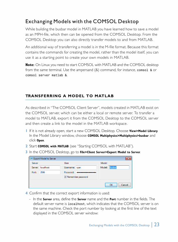
3 In the COMSOL Desktop, go to File>Client Server>Export Model to Server.
4 Confirm that the correct export information is used:
- In the Server area, define the Server name and the Port number in the fields. The default server name is localhost, which indicates that the COMSOL server is on the same machine. Check the port number by looking at the first line of the text displayed in the COMSOL server window:
Exchanging Models with the COMSOL Desktop | 23

COMSOL 4.3 started listening on port 2036
- The User area contains the user login information. The Username and Password fields are set by default based on settings in the user preferences, defined the first time a COMSOL server is started.
- The Model area contains the Model field where the model object name can be defined to export it from the COMSOL server. For this example enter Busbar
5 Click OK.
Now that the model object is stored in the COMSOL server, create a link in MATLAB to gain access to it.
6 Once the Export model to server window has closed, enter at the MATLAB command line:model = ModelUtil.model('Busbar');
Busbar is the model object name, which was defined in step 4 above.
7 All features of the model can now be accessed, for example, plot the second plot group in a MATLAB figure:mphplot(model,'pg2','rangenum',1)
8 The model can also be modified, for example, by removing the second plot group from the results node:model.result.remove('pg2');
TRANSFERRING A MODEL TO THE COMSOL DESKTOP
As well as transferring your model to MATLAB, the model edited at the MATLAB command line can be transferred to the COMSOL server. It only requires to load the model object from the COMSOL server to the COMSOL Desktop.
1 Start COMSOL with MATLAB and a COMSOL Desktop.
2 Create a model object, then create a 3D geometry and draw a block:model = ModelUtil.create('ImportExample');model.geom.create('geom1', 3);
24 | Exchanging Models with the COMSOL Desktop
model.geom('geom1').feature.create('blk1', 'Block');model.geom('geom1').run;
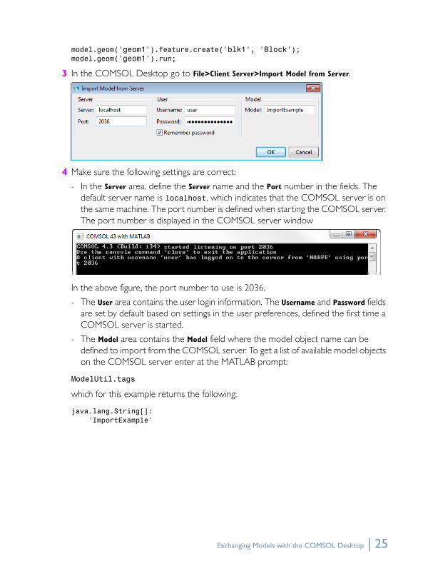
3 In the COMSOL Desktop go to File>Client Server>Import Model from Server.
4 Make sure the following settings are correct:
- In the Server area, define the Server name and the Port number in the fields. The default server name is localhost, which indicates that the COMSOL server is on the same machine. The port number is defined when starting the COMSOL server. The port number is displayed in the COMSOL server window
In the above figure, the port number to use is 2036.
- The User area contains the user login information. The Username and Password fields are set by default based on settings in the user preferences, defined the first time a COMSOL server is started.
- The Model area contains the Model field where the model object name can be defined to import from the COMSOL server. To get a list of available model objects on the COMSOL server enter at the MATLAB prompt:
ModelUtil.tags
which for this example returns the following:
java.lang.String[]: 'ImportExample'
Exchanging Models with the COMSOL Desktop | 25
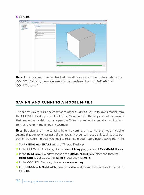
5 Click OK.
Note: It is important to remember that if modifications are made to the model in the COMSOL Desktop, the model needs to be transferred back to MATLAB (the COMSOL server).
SAVING AND RUNNING A MODEL M-FILE
The easiest way to learn the commands of the COMSOL API is to save a model from the COMSOL Desktop as an M-file. The M-file contains the sequence of commands that create the model. You can open the M-file in a text editor and do modifications to it, as shown in the following example.
Note: By default the M-file contains the entire command history of the model, including settings that are no longer part of the model. In order to include only settings that are part of the current model, you need to reset the model history before saving the M-file.
1 Start COMSOL with MATLAB and a COMSOL Desktop.
2 In the COMSOL Desktop go to the Model Library page, or select View>Model Library.
3 In the Model Library window, expand the COMSOL Multiphysics folder and then the Multiphysics folder. Select the busbar model and click Open.
4 In the COMSOL Desktop, choose File>Reset History.
5 Go to File>Save As Model M-File, name it busbar and choose the directory to save it to. Click OK.
26 | Exchanging Models with the COMSOL Desktop

6 Open the saved M-file with the MATLAB editor or any text editor and scroll to lines 184–188: model.result('pg3').feature('surf1').set('expr','jh.normJ');model.result('pg3').feature('surf1').set('rangecolormax','1e6')
The commands above define the plot group pg2. According to line 184 it includes a surface plot of the expression to jh.normJ. On line 188 the maximum color range is set to 1e6.
7 Modify the plot group pg2 so that it displays the total heat jh.Qtot and set the maximum color range to 1e4 instead. Starting on a new line right after line 188, append the following to the M-file:
model.result('pg2').feature('surf1').set('expr','jh.Qtot');model.result('pg2').feature('surf1').set('rangecolormax','1e4');
These commands are executed after lines 184–188 and modify plot group pg2 so that it displays the total heat jh.qtot with a new setting for the maximum value for the color range. Line 184 and 188 can also be modified to achieve the same thing, but this way you can easily revert to the old version.
8 Save the modified M-file.
9 Run the model at the MATLAB prompt with the command:model = busbar;
10Display the plot group pg2:mphplot(model,'pg2','rangenum',1)
Another way to modify a model object in MATLAB is to export the model from the COMSOL Desktop to MATLAB (see “Transferring a Model to MATLAB”) and then enter the commands in step 5 directly at the MATLAB command line. The benefit of this latter approach is that it does not require running the entire model. See “An Example Using Multiple for Loops”, where this technique is applied.
Exchanging Models with the COMSOL Desktop | 27

Extracting Results at the MATLAB Command LineLiveLink for MATLAB packages several functions to make it easy to access results directly from the MATLAB command line. These functions are:
• mpheval, to evaluate expressions on all node points of a given domain selection,
• mphinterp, to evaluate expressions at extracts data arbitrary location,
• mphglobal, to evaluate global expressions,
• mphint, to integrate value of expressions on selected domains.
Load the model busbar from the Model library directly at the MATLAB command line.
1 Start COMSOL with MATLAB.
2 Load the busbar example model from the Model Library. Enter the command:model = mphload('busbar');
The mphload command automatically searches the COMSOL path to find the requested file. You can also specify the path in the file name.
EVALUATING DATA AT NODE POINTS
Use the mpheval function to evaluate the electric potential, which is one of the busbar model dependent variables. mpheval returns the value of the expression evaluated using the nodes of a simplex mesh. By default the simplex mesh corresponds to the active mesh in the model object.
1 Enter at the command line:data = mpheval(model,'V')
A MATLAB structure is returned according to:data = expr: {'V'} d1: [1x1787 double] p: [3x1787 double] t: [4x6416 int32] ve: [1787x1 int32] unit: {'V'}
28 | Extracting Results at the MATLAB Command Line
mpheval returns a MATLAB structure defined with the following fields:
- expr contains the list of the evaluated expression,
- d1 contains the data of the evaluated expression,
- p contains the coordinates of the evaluation points,
- t contains the indices to columns in the p field. Each column in the t field corresponds to an element of the mesh used for the evaluation,
- ve contains the indices of the mesh elements at each evaluation point,
- unit contains the unit of the evaluated expression.
2 Multiple variables can be evaluated at once, for example both the temperature and the electric potential. Enter:data2 = mpheval(model,{'T' 'V'})
This command returns this structure:data2 = expr: {'T' 'V'} d1: [1x1787 double] d2: [1x1787 double] p: [3x1787 double] t: [4x6416 int32] ve: [1787x1 int32] unit: {'K' 'V'}
The fields data2.d1 and data2.d2 contain the values for the temperature and electric potential, respectively.
3 Now evaluate the temperature T including at the element mid-points as defined by a quadratic shape function. Use the refine property and set the property value to 2, which corresponds to the discretization order :data3 = mpheval(model,{'T'},'refine',2)
This command returns this structure:data3 = expr: {'T'} d1: [1x11304 double] p: [3x11304 double] t: [4x51328 int32] ve: [11304x1 int32] unit: {'K'}
4 This step tests how to use the edim property in combination with the selection property. edim allows you to determine the space dimension of the evaluation and selection allows you to set the entity number where to evaluate the expression.
Evaluate data on a specific domain, for example the normal current density at boundary number 43:
Extracting Results at the MATLAB Command Line | 29

data4 = mpheval(model,{'jh.normJ'},... 'edim',2,'selection',43)
This command returns this structure:data4 = expr: {'jh.normJ'} d1: [1x36 double] p: [3x36 double] t: [3x54 int32] ve: [36x1 int32] unit: {'A/m^2'}
EVALUATING DATA AT ARBITRARY POINTS
If you want to get data at a specific location not necessarily defined by node points, use the command mphinterp to interpolate the results. The interpolation method uses the shape function of the elements.
1 To extract the total heat source at [5e-2;-2e-2;1e-3] enter:Qtot = mphinterp(model,'jh.Qtot','coord',[5e-2;-2e-2;1e-3])
This returns:Qtot = 7.0214e+003
2 A grid of points can also be evaluated. Enter the following lines:x0=0:5e-2/4:5e-2;y0=0:-2.5e-2/4:-2.5e-2;z0=[0 5e-3];[x,y,z]=meshgrid(x0,y0,z0);xx=[x(:),y(:),z(:)]';Qtot = mphinterp(model,'jh.Qh','coord',xx);
3 Reshape the variable Qtot for a better visualization:Qtot = reshape(Qtot,length(x0),length(y0),length(z0))
This results in:Qtot(:,:,1) =1.0e+005 * 0.0000 0.0288 0.0742 0.0705 0.0702 0.0008 0.2894 0.0755 0.0702 0.0702 0.0000 3.1122 0.0688 0.0699 0.0702 0.0006 0.2660 0.0731 0.0702 0.0702 0.0000 0.0281 0.0747 0.0705 0.0702
Qtot(:,:,2) =1.0e+003 *
30 | Extracting Results at the MATLAB Command Line
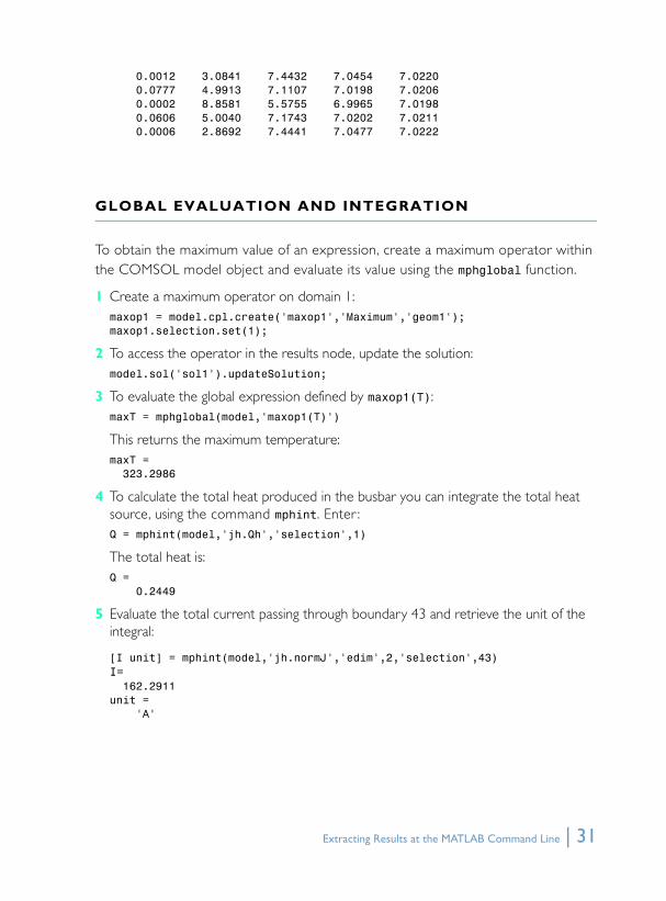
0.0012 3.0841 7.4432 7.0454 7.0220 0.0777 4.9913 7.1107 7.0198 7.0206 0.0002 8.8581 5.5755 6.9965 7.0198 0.0606 5.0040 7.1743 7.0202 7.0211 0.0006 2.8692 7.4441 7.0477 7.0222
GLOBAL EVALUATION AND INTEGRATION
To obtain the maximum value of an expression, create a maximum operator within the COMSOL model object and evaluate its value using the mphglobal function.
1 Create a maximum operator on domain 1:maxop1 = model.cpl.create('maxop1','Maximum','geom1');maxop1.selection.set(1);
2 To access the operator in the results node, update the solution:model.sol('sol1').updateSolution;
3 To evaluate the global expression defined by maxop1(T):maxT = mphglobal(model,'maxop1(T)')
This returns the maximum temperature:maxT = 323.2986
4 To calculate the total heat produced in the busbar you can integrate the total heat source, using the command mphint. Enter :Q = mphint(model,'jh.Qh','selection',1)
The total heat is:Q = 0.2449
5 Evaluate the total current passing through boundary 43 and retrieve the unit of the integral:
[I unit] = mphint(model,'jh.normJ','edim',2,'selection',43)I= 162.2911unit = 'A'
Extracting Results at the MATLAB Command Line | 31

Automating with MATLAB ScriptsThe LiveLink interface allows you to combine the MATLAB programing tools with the COMSOL model object. A benefit of this integration is to access results at the MATLAB workspace. Another benefit is that you can integrate COMSOL modeling commands into MATLAB scripts, taking full advantage of all available tools for controlling the flow of your code. This section explains how to do this efficiently by introducing MATLAB variables into your COMSOL model and updating only the affected parts of your model object.
OBTAINING MODEL INFORMATION
Modifying an existing model object requires you to know how the model is set up. Some functions help you to access this information so that you can add or remove a model feature or modify the value of an existing property. The function mphnavigator helps you to retrieve model object information. Calling mphnavigator at the MATLAB prompt displays a summary of the features and their proper ties for the model object available in the MATLAB workspace.
1 Start COMSOL with MATLAB.
1 Load the busbar example model:model=mphload('busbar');
2 To access the model information, enter the following command at the MATLAB prompt:mphnavigator
32 | Automating with MATLAB Scripts

In the mphnavigator graphical user interface the model features are listed under the Model Tree section. The nodes can be expanded to access the subfeatures. When selecting a feature from the Model Tree, its properties are listed under the Properties section. The Methods section lists the method available for the selected feature. Just above the Methods section, you can see the COMSOL API syntax that lead to the feature. You can copy the command to the clipboard and easily paste it at the MATLAB prompt—just press the Copy button to copy the syntax.
3 In the Model Tree, expand the model feature nodes down to geom>geom1>wp1>r1 and select the node r1.
4 In the Properties section, you can see the that the lx property of the geometry feature r1 is set to L+2*tbb, this represent the length of the rectangle. The width of the rectangle, represented with the property ly is set to 0.1.
Automating with MATLAB Scripts | 33
UPDATING MODEL SETTINGS
The COMSOL model object allows you to modify parameters, features, or feature properties, using the set method. Once a property value is updated, you can run the appropriate sequence, depending on where the changes where introduced into the model—for example, the geometry or the mesh sequence. Running the solver sequence automatically runs all sequences where modified settings are detected.
Star ting with the busbar model described in “A Thorough Example: The Busbar”, this section modifies a parameter value and re-solves the model. For this purpose, the geometry of the model is prepared using parameters such as L, the length of the busbar, and tbb, the thickness of the busbar.
1 Start COMSOL with MATLAB (if you have not done so already).
2 Load the model from the COMSOL model library:model = mphload('busbar');
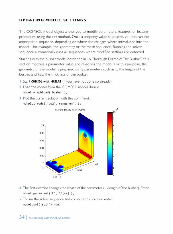
3 Plot the current solution with this command:mphplot(model,'pg2','rangenum',1);
4 The first exercise changes the length of the parameters L (length of the busbar). Enter :model.param.set('L','18[cm]');
5 To run the solver sequence and compute the solution enter:model.sol('sol1').run;
34 | Automating with MATLAB Scripts

Note: The solver node automatically detects all modifications in the model, and runs the geometry or mesh sequences when needed. Here, the new value for the parameter L induces a change in the geometry and thus a new mesh is also needed. Full associativity is also ensured making sure that all physics settings remain applied as in the original model.
6 Plot the updated solution, which results in the geometry change: mphplot(model,'pg2','rangenum',1);
USING MATLAB VARIABLES IN THE COMSOL MODEL
Use the set method described in the previous section to define the feature properties using MATLAB variables. It is important to make sure that the value of the MATLAB variable is consistent with the units used in the model. Before beginning, make sure that the busbar model used in the previous section is loaded into MATLAB.
First, change the length of the busbar, described by the parameter L.
1 Create a MATLAB variable L0 equal to 9e-2:L0 = 9e-2;
2 Update the value of the parameter L with the variable L0:model.param.set('L',L0);
Automating with MATLAB Scripts | 35
Note: In contrast to this command, setting a value using an expression from within the model object requires the second argument to be a string expression, as shown in “Updating Model Settings”.
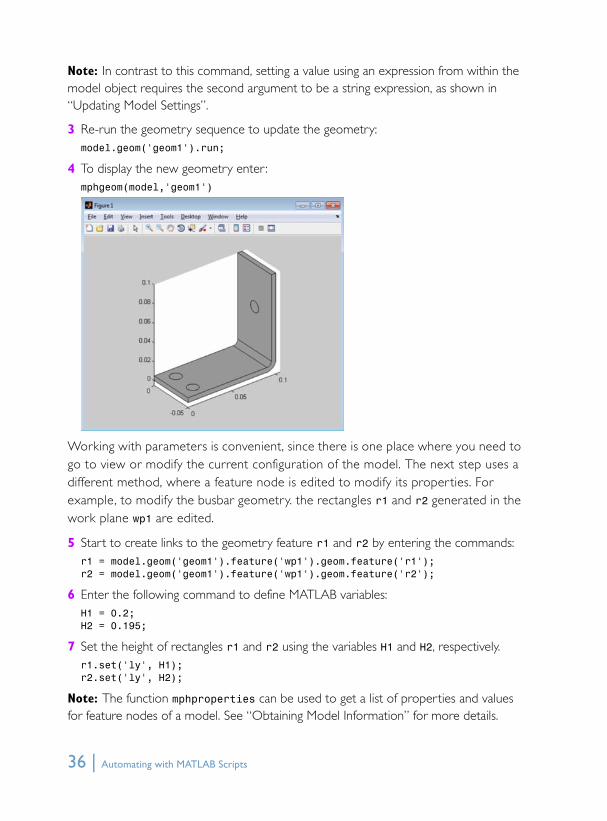
3 Re-run the geometry sequence to update the geometry:model.geom('geom1').run;
4 To display the new geometry enter:mphgeom(model,'geom1')
Working with parameters is convenient, since there is one place where you need to go to view or modify the current configuration of the model. The next step uses a different method, where a feature node is edited to modify its properties. For example, to modify the busbar geometry. the rectangles r1 and r2 generated in the work plane wp1 are edited.
5 Start to create links to the geometry feature r1 and r2 by entering the commands:r1 = model.geom('geom1').feature('wp1').geom.feature('r1');r2 = model.geom('geom1').feature('wp1').geom.feature('r2');
6 Enter the following command to define MATLAB variables:H1 = 0.2;H2 = 0.195;
7 Set the height of rectangles r1 and r2 using the variables H1 and H2, respectively.r1.set('ly', H1);r2.set('ly', H2);
Note: The function mphproperties can be used to get a list of properties and values for feature nodes of a model. See “Obtaining Model Information” for more details.
36 | Automating with MATLAB Scripts

8 To update the geometry, enter:model.geom('geom1').run;
9 Enter this command to plot the geometry:mphgeom(model,'geom1');
There is a third option when defining property values for features: to combine MATLAB variables with parameters or variables defined within the COMSOL model object. To do this the MATLAB variable just needs to be converted to a string.
This last exercise tests this by changing the height of rectangle r1 and r2 to L0, and L0-tbb, respectively, where L0 is a MATLAB variable.
10Define the variable L0:L0 = 0.1;
11Modify the ly property of rectangles r1 and r2:r1.set('ly',L0)r2.set('ly',[num2str(L0) '-tbb']);
Automating with MATLAB Scripts | 37

12Update and plot the geometry:model.geom('geom1').run;mphgeom(model,'geom1');
AN EXAMPLE USING MULTIPLE FOR LOOPS
In this example, a MATLAB function is created that solves the busbar model for different values of the length and thickness of the busbar, and the input electric potential. The function evaluates and returns the maximum temperature in the busbar, the generated heat, and the current through the busbar. For each variation of the model the function stores these results in a file and saves the model object in a MPH file. To make it easy to identify the name of the MPH-file, it contains the values of the different parameters used to set-up the model.
The input argument of the M-function is the busbar model object and the path to the directory where the data and models are saved.
1 Open a text editor, for example the MATLAB text editor.
2 At the first line of a new M-file, enter the following function header :function modelParam(model,filepath)
The function first creates a file and then sets the header of the output file format.
38 | Automating with MATLAB Scripts

3 In the text editor continue to enter the following lines:filename = fullfile(filepath,'results.txt');fid=fopen(filename,'wt');fprintf(fid,'*** run parametric study ***\n');fprintf(fid,'L[m] | tbb[m] | Vtot[V] | ');fprintf(fid,'MaxT[K] | TotQ[W] | Current[A]\n');
4 In order to evaluate the maximum values add a coupling operator to the model. Enter the lines:maxop1 = model.cpl.create('maxop1','Maximum','geom1');maxop1.selection.set(1);
5 When running a large amount of iteration, the model history can be disabled to prevent the memory from rising along the iterations due to the model history stored in the model. Enter the lines:model.hist.disable;
6 Now start a for loop to parameterize the parameter L and set the corresponding parameter in the model object. Enter the commands:for L = [9e-2 15e-2]model.param.set('L',L);
7 Continue by creating a second for loop, this time to parameterize the parameter tbb and to modify its value in the model object:for tbb = [5e-3 10e-3]model.param.set('tbb',tbb);
8 Define the last for loop to parameterize the applied potential Vtot:for Vtot = [20e-3 40e-3]model.param.set('Vtot',Vtot);
9 For each version of the model write the parameter values to the output file:fprintf(fid,[num2str(L),' | ',num2str(tbb),...' | ',num2str(Vtot),' | ']);
10To solve the model, add the line below:model.sol('sol1').run;
11The following lines evaluate the results:MaxT = mphglobal(model,'maxop1(T)');TotQ = mphint(model,'jh.Qtot','selection',1);Current = mphint(model,'jh.normJ',...'edim',2,'selection',43);
12Save the results to the output text file:fprintf(fid,[num2str(MaxT),' | ',num2str(TotQ),...' | ',num2str(Current),' \n']);
Automating with MATLAB Scripts | 39

13Name and save the model:modelName = fullfile(filepath,['busbar_L=',num2str(L),...'_tbb=',num2str(tbb),...'_Vtot=',num2str(Vtot),'.mph']);model.save(modelName);
14Terminate the for loops:endendend
15Close the output text file:fclose(fid);
The script in the text editor should now look like this text:
function modelParam(model,filepath)filename = fullfile(filepath,'results.txt');fid=fopen(filename,'wt');fprintf(fid,'*** run parametric study ***\n');fprintf(fid,'L[m] | tbb[m] | Vtot[V] | ');fprintf(fid,'MaxT[K] | TotQ[W] | Current[A]\n');maxop1 = model.cpl.create('maxop1','Maximum','geom1');maxop1.selection.set(1);model.hist.disable;for L = [9e-2 15e-2] model.param.set('L',L); for tbb = [5e-3 10e-3] model.param.set('tbb',tbb); for Vtot = [20e-3 40e-3] model.param.set('Vtot',Vtot); fprintf(fid,[num2str(L),' | ',num2str(tbb),... ' | ',num2str(Vtot),' | ']); model.sol('sol1').run; MaxT = mphglobal(model,'maxop1(T)'); TotQ = mphint(model,'jh.Qtot','selection',1); Current = mphint(model,'jh.normJ',... 'edim',2,'selection',43); fprintf(fid,[num2str(MaxT),' | ',num2str(TotQ),... ' | ',num2str(Current),' \n']); modelName = fullfile(filepath,['busbar_L=',num2str(L),... '_tbb=',num2str(tbb),... '_Vtot=',num2str(Vtot),'.mph']); model.save(modelName); end endendfclose(fid);
16Save the M-file as modelParam.m in a directory known by MATLAB.
40 | Automating with MATLAB Scripts
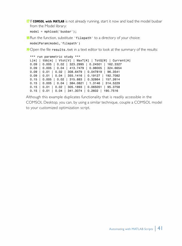
17 If COMSOL with MATLAB is not already running, start it now and load the model busbar from the Model library:model = mphload('busbar');
18Run the function, substitute 'filepath' to a directory of your choice:modelParam(model,'filepath')
19Open the file results.txt in a text editor to look at the summary of the results:
*** run parametric study ***L[m] | tbb[m] | Vtot[V] | MaxT[K] | TotQ[W] | Current[A]0.09 | 0.005 | 0.02 | 323.2995 | 0.24501 | 162.3327 0.09 | 0.005 | 0.04 | 413.7479 | 0.98005 | 324.6654 0.09 | 0.01 | 0.02 | 308.6479 | 0.047819 | 96.3541 0.09 | 0.01 | 0.04 | 355.1416 | 0.19127 | 192.7082 0.15 | 0.005 | 0.02 | 315.883 | 0.32864 | 157.2614 0.15 | 0.005 | 0.04 | 384.0821 | 1.3146 | 314.5229 0.15 | 0.01 | 0.02 | 305.1893 | 0.065051 | 95.3758 0.15 | 0.01 | 0.04 | 341.3074 | 0.2602 | 190.7516
Although this example duplicates functionality that is readily accessible in the COMSOL Desktop, you can, by using a similar technique, couple a COMSOL model to your customized optimization script.
Automating with MATLAB Scripts | 41
Using External MATLAB FunctionsAnother advantage of using LiveLink for MATLAB is the ability to call a MATLAB function directly from within the COMSOL Desktop. You can use the function to define, within the COMSOL model object, proper ties such as material definitions or physics settings. COMSOL automatically detects the external function and star ts the MATLAB engine to evaluate it. The function output is then applied to the corresponding proper ty.
To use this functionality, just star t the COMSOL Desktop and MATLAB automatically star ts in the background when needed.
Note: On Linux operating systems, specify the MATLAB root directory path MLROOT and load the gcc library when starting the COMSOL Desktop: comsol -mlroot MLROOT -forcegcc.
The example in this section illustrates how to use external MATLAB functions in a COMSOL model. The model computes for the temperature distribution in a material subjected to an external heat flux. Both the thermal conductivity of the material and the applied heat flux are defined by MATLAB functions.
CREATING THE MATLAB FUNCTIONS
Assume that the material in the example is characterized by a random thermal conductivity. To define the thermal conductivity, create a MATLAB function with the location along the x-axis as an input argument and let the conductivity vary randomly within 200 W/(m*K) around a constant value of 400 W/(m*K).
Define a second MATLAB function for the external heat flux to be a function of the following arguments:
• x and y, the location coordinates.
• x0 and y0, the coordinates of the center of application of the heat source.
• Q0, the maximum heat source.
• scale, a parameter that scale the period of the heat flux.
x and y are dependent variables of the model. x0, y0, Q0, and scale are defined with constant value in this exercise.
42 | Using External MATLAB Functions
1 Open a text editor, for example the MATLAB text editor.
2 In a new file enter:function out=conductivity(x)out = 400+5*randn(size(x));
3 Save the file as conductivity.m.
4 Create a new file and enter:function out = heatflux(x,y,x0,y0,Q0,scale)radius = sqrt((x-x0).^2+(y-y0).^2);out = Q0/5+Q0/2.*sin(scale*pi.*radius)./(scale*pi.*radius);
5 Save the file as HeatFlux.m.
Note: For both functions the input arguments have the size of the space coordinate variables x and y. These variables are defined as arrays, and the function needs to return an array with the same size as the input arguments. Ensure that this is the case by using the size command and pointwise operators (.* and ./).
MODEL WIZARD
1 Start COMSOL Multiphysics.
2 In the Model Wizard window, on the Select Space Dimension page, select 3D. Click Next .
3 On the Add Physics page, select Heat Transfer > Heat Transfer in Solids(ht). Click Next .
4 On the Select Study Type page, under Preset Studies select Stationary .
5 Click Finish .
DEFINING THE EXTERNAL MATLAB FUNCTIONS IN THE MODEL
You have noticed that the two MATLAB functions are highlighted in orange after being entered. This is because they need to be defined in the model before COMSOL can recognize them as external MATLAB functions.
Using External MATLAB Functions | 43

1 Right-click Global Definitions node and select Functions > MATLAB.
2 On the Settings page, under the Functions section in the Function field enter conductivity and under the Arguments field enter x.
By defining the function here, COMSOL knows that conductivity is a MATLAB function. COMSOL automatically star ts MATLAB to evaluate the function when necessary.
Note: Saving the COMSOL model at the location (as for the external MATLAB functions) ensures that the functions path is known by MATLAB. Other alternatives consist in setting the function path directly in MATLAB before running the model or setting the environment variable COMSOL_MATLAB_PATH with the directory path of the functions.
3 Go to the File menu, select Save As, and browse to the directory where the files conductivity.m and heatflux.m are stored.
You can display the value of the function defined by first defining the plot limit for the input arguments.
4 Expand the Plot parameters section. In the associated table enter 0 as Lower limit and 1 as Upper limit.
44 | Using External MATLAB Functions

5 Click the Plot button .
You can now define a second MATLAB function that returns the heat flux condition.
6 Repeating the above procedure, add a new MATLAB function. On the Settings page under Functions section, enter heatflux in the Function field and set the Arguments field with x,y,x0,y0,scale.
7 To display the function enter the following in the Plot parameters table:
LOWER LIMIT UPPER LIMIT
0 1
0 1
0 0
0 0
Using External MATLAB Functions | 45
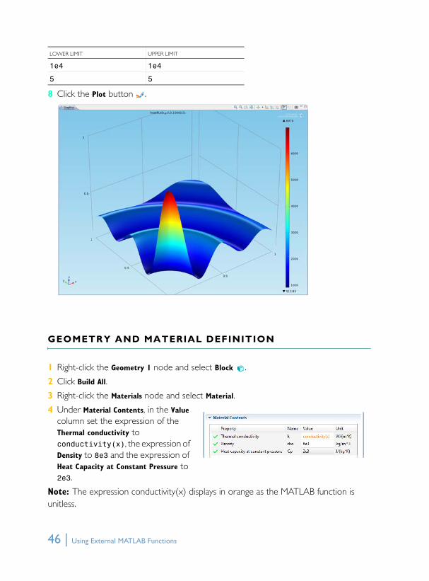
8 Click the Plot button .
GEOMETRY AND MATERIAL DEFINITION
1 Right-click the Geometry 1 node and select Block .
2 Click Build All.
3 Right-click the Materials node and select Material.
4 Under Material Contents, in the Value column set the expression of the Thermal conductivity to conductivity(x), the expression of Density to 8e3 and the expression of Heat Capacity at Constant Pressure to 2e3.
Note: The expression conductivity(x) displays in orange as the MATLAB function is unitless.
1e4 1e4
5 5
LOWER LIMIT UPPER LIMIT
46 | Using External MATLAB Functions

HEAT TRANSFER IN SOLIDS
1 Add a constant temperature boundary condition. Right-click Heat Transfer in Solids, then select Temperature.
2 On the Temperature settings page, select boundaries 3, 5, and 6 (You can also use the Paste Selection button to enter directly the selection).
3 To add a boundary heat flux right-click Heat Transfer in Solids node, and select Heat Flux.
4 On the Heat flux settings page select boundary 4 and set the General inward heat flux expression to heatflux(x,y,0.5,0.5,1e4,3).
COMPUTING AND PLOTTING THE RESULTS
Once the model is set-up the solution can be computed. A default mesh is automatically generated.
1 Right-click the Study node and select Compute .
2 Click the Temperature (ht) node to display the temperature field at the geometry surface.
Using External MATLAB Functions | 47

3 Visualize the material thermal conductivity in the geometry by adding a new 3D Plot group in the Results node. Then right-click 3D Plot group 3 node and select Isosurface .
4 On the associated Settings page, under the Expression section, enter conductivity(x) in the Expression field.
5 Under Levels section change the Total levels to 15.
6 Click the Plot button .
48 | Using External MATLAB Functions