INTRODUCTION TO LATTICE THEORY WITH COMPUTER …
244
INTRODUCTION TO LATTICE THEORY WITH COMPUTER SCIENCE APPLICATIONS
Transcript of INTRODUCTION TO LATTICE THEORY WITH COMPUTER …

INTRODUCTION TOLATTICE THEORY WITHCOMPUTER SCIENCEAPPLICATIONS

INTRODUCTION TOLATTICE THEORY WITHCOMPUTER SCIENCEAPPLICATIONS
VIJAY K. GARGDepartment of Electrical and Computer EngineeringThe University of Texas at Austin

Copyright © 2015 by John Wiley & Sons, Inc. All rights reserved
Published by John Wiley & Sons, Inc., Hoboken, New JerseyPublished simultaneously in Canada
No part of this publication may be reproduced, stored in a retrieval system, or transmitted in any form orby any means, electronic, mechanical, photocopying, recording, scanning, or otherwise, except aspermitted under Section 107 or 108 of the 1976 United States Copyright Act, without either the priorwritten permission of the Publisher, or authorization through payment of the appropriate per-copy fee tothe Copyright Clearance Center, Inc., 222 Rosewood Drive, Danvers, MA 01923, (978) 750-8400, fax(978) 750-4470, or on the web at www.copyright.com. Requests to the Publisher for permission shouldbe addressed to the Permissions Department, John Wiley & Sons, Inc., 111 River Street, Hoboken, NJ07030, (201) 748-6011, fax (201) 748-6008, or online at http://www.wiley.com/go/permission.
Limit of Liability/Disclaimer of Warranty: While the publisher and author have used their best efforts inpreparing this book, they make no representations or warranties with respect to the accuracy orcompleteness of the contents of this book and specifically disclaim any implied warranties ofmerchantability or fitness for a particular purpose. No warranty may be created or extended by salesrepresentatives or written sales materials. The advice and strategies contained herein may not be suitablefor your situation. You should consult with a professional where appropriate. Neither the publisher norauthor shall be liable for any loss of profit or any other commercial damages, including but not limited tospecial, incidental, consequential, or other damages.
For general information on our other products and services or for technical support, please contact ourCustomer Care Department within the United States at (800) 762-2974, outside the United States at(317) 572-3993 or fax (317) 572-4002.
Wiley also publishes its books in a variety of electronic formats. Some content that appears in print maynot be available in electronic formats. For more information about Wiley products, visit our web site atwww.wiley.com.
Library of Congress Cataloging-in-Publication Data:
Garg, Vijay K. (Vijay Kumar), 1963-Introduction to lattice theory with computer science applications / Vijay K. Garg.
pages cmIncludes bibliographical references and index.ISBN 978-1-118-91437-3 (cloth)1. Computer science–Mathematics. 2. Engineering mathematics. 3. Lattice theory. I. Title.QA76.9.L38G37 2015004.01′51–dc23
2015003602Printed in the United States of America
10 9 8 7 6 5 4 3 2 1
1 2015

To my family

CONTENTS
List of Figures xiii
Nomenclature xix
Preface xxi
1 Introduction 1
1.1 Introduction, 11.2 Relations, 21.3 Partial Orders, 31.4 Join and Meet Operations, 51.5 Operations on Posets, 71.6 Ideals and Filters, 81.7 Special Elements in Posets, 91.8 Irreducible Elements, 101.9 Dissector Elements, 111.10 Applications: Distributed Computations, 111.11 Applications: Combinatorics, 121.12 Notation and Proof Format, 131.13 Problems, 151.14 Bibliographic Remarks, 15

viii CONTENTS
2 Representing Posets 17
2.1 Introduction, 172.2 Labeling Elements of The Poset, 172.3 Adjacency List Representation, 182.4 Vector Clock Representation, 202.5 Matrix Representation, 222.6 Dimension-Based Representation, 222.7 Algorithms to Compute Irreducibles, 232.8 Infinite Posets, 242.9 Problems, 262.10 Bibliographic Remarks, 27
3 Dilworth’s Theorem 29
3.1 Introduction, 293.2 Dilworth’s Theorem, 293.3 Appreciation of Dilworth’s Theorem, 303.4 Dual of Dilworth’s Theorem, 323.5 Generalizations of Dilworth’s Theorem, 323.6 Algorithmic Perspective of Dilworth’s Theorem, 323.7 Application: Hall’s Marriage Theorem, 333.8 Application: Bipartite Matching, 343.9 Online Decomposition of Posets, 353.10 A Lower Bound on Online Chain Partition, 373.11 Problems, 383.12 Bibliographic Remarks, 39
4 Merging Algorithms 41
4.1 Introduction, 414.2 Algorithm to Merge Chains in Vector Clock Representation, 414.3 An Upper Bound for Detecting an Antichain of Size K, 474.4 A Lower Bound for Detecting an Antichain of Size K, 484.5 An Incremental Algorithm for Optimal Chain Decomposition, 504.6 Problems, 504.7 Bibliographic Remarks, 51
5 Lattices 53
5.1 Introduction, 535.2 Sublattices, 545.3 Lattices as Algebraic Structures, 555.4 Bounding The Size of The Cover Relation of a Lattice, 565.5 Join-Irreducible Elements Revisited, 57

CONTENTS ix
5.6 Problems, 595.7 Bibliographic Remarks, 60
6 Lattice Completion 61
6.1 Introduction, 616.2 Complete Lattices, 616.3 Closure Operators, 626.4 Topped ∩-Structures, 636.5 Dedekind–Macneille Completion, 646.6 Structure of Dedekind—Macneille Completion of a Poset, 676.7 An Incremental Algorithm for Lattice Completion, 696.8 Breadth First Search Enumeration of Normal Cuts, 716.9 Depth First Search Enumeration of Normal Cuts, 736.10 Application: Finding the Meet and Join of Events, 756.11 Application: Detecting Global Predicates in Distributed Systems, 766.12 Application: Data Mining, 776.13 Problems, 786.14 Bibliographic Remarks, 78
7 Morphisms 79
7.1 Introduction, 797.2 Lattice Homomorphism, 797.3 Lattice Isomorphism, 807.4 Lattice Congruences, 827.5 Quotient Lattice, 837.6 Lattice Homomorphism and Congruence, 837.7 Properties of Lattice Congruence Blocks, 847.8 Application: Model Checking on Reduced Lattices, 857.9 Problems, 897.10 Bibliographic Remarks, 90
8 Modular Lattices 91
8.1 Introduction, 918.2 Modular Lattice, 918.3 Characterization of Modular Lattices, 928.4 Problems, 988.5 Bibliographic Remarks, 98
9 Distributive Lattices 99
9.1 Introduction, 999.2 Forbidden Sublattices, 99

x CONTENTS
9.3 Join-Prime Elements, 1009.4 Birkhoff’s Representation Theorem, 1019.5 Finitary Distributive Lattices, 1049.6 Problems, 1049.7 Bibliographic Remarks, 105
10 Slicing 107
10.1 Introduction, 10710.2 Representing Finite Distributive Lattices, 10710.3 Predicates on Ideals, 11010.4 Application: Slicing Distributed Computations, 11610.5 Problems, 11710.6 Bibliographic Remarks, 118
11 Applications of Slicing to Combinatorics 119
11.1 Introduction, 11911.2 Counting Ideals, 12011.3 Boolean Algebra and Set Families, 12111.4 Set Families of Size k, 12211.5 Integer Partitions, 12311.6 Permutations, 12711.7 Problems, 12911.8 Bibliographic Remarks, 129
12 Interval Orders 131
12.1 Introduction, 13112.2 Weak Order, 13112.3 Semiorder, 13312.4 Interval Order, 13412.5 Problems, 13612.6 Bibliographic Remarks, 137
13 Tractable Posets 139
13.1 Introduction, 13913.2 Series–Parallel Posets, 13913.3 Two-Dimensional Posets, 14213.4 Counting Ideals of a Two-Dimensional Poset, 14513.5 Problems, 14713.6 Bibliographic Remarks, 147

CONTENTS xi
14 Enumeration Algorithms 149
14.1 Introduction, 14914.2 BFS Traversal, 15014.3 DFS Traversal, 15414.4 LEX Traversal, 15414.5 Uniflow Partition of Posets, 16014.6 Enumerating Tuples of Product Spaces, 16314.7 Enumerating All Subsets, 16314.8 Enumerating All Subsets of Size k, 16514.9 Enumerating Young’s Lattice, 16614.10 Enumerating Permutations, 16714.11 Lexical Enumeration of All Order Ideals of a Given Rank, 16814.12 Problems, 17214.13 Bibliographic Remarks, 173
15 Lattice of Maximal Antichains 175
15.1 Introduction, 17515.2 Maximal Antichain Lattice, 17715.3 An Incremental Algorithm Based on Union Closure, 17915.4 An Incremental Algorithm Based on BFS, 18115.5 Traversal of the Lattice of Maximal Antichains, 18215.6 Application: Detecting Antichain-Consistent Predicates, 18415.7 Construction and Enumeration of Width Antichain Lattice, 18515.8 Lexical Enumeration of Closed Sets, 18715.9 Construction of Lattices Based on Union Closure, 19015.10 Problems, 19015.11 Bibliographic Remarks, 191
16 Dimension Theory 193
16.1 Introduction, 19316.2 Chain Realizers, 19416.3 Standard Examples of Dimension Theory, 19516.4 Relationship Between the Dimension and the Width of a Poset, 19616.5 Removal Theorems for Dimension, 19716.6 Critical Pairs in the Poset, 19816.7 String Realizers, 19916.8 Rectangle Realizers, 20916.9 Order Decomposition Method and Its Applications, 21016.10 Problems, 21216.11 Bibliographic Remarks, 213

xii CONTENTS
17 Fixed Point Theory 215
17.1 Complete Partial Orders, 21517.2 Knaster–Tarski Theorem, 21617.3 Application: Defining Recursion Using Fixed Points, 21817.4 Problems, 22617.5 Bibliographic Remarks, 227
Bibliography 229
Index 235

LIST OF FIGURES
Figure 1.1 The graph of a relation 2
Figure 1.2 Hasse diagram 4
Figure 1.3 Only the first two posets are lattices 5
Figure 1.4 (a) Pentagon(N5) and (b) diamond(M3) 7
Figure 1.5 Cross product of posets 8
Figure 1.6 A computation in the happened-before model 12
Figure 1.7 Ferrer’s diagram for (4, 3, 2) shown to contain (2, 2, 2) 13
Figure 1.8 Young’s lattice for (3, 3, 3) 14
Figure 2.1 Adjacency list representation of a poset 19
Figure 2.2 Vector clock labeling of a poset for a distributed computation 21
Figure 2.3 Vector clock algorithm 22
Figure 2.4 (a) An antichain of size 5 and (b) its two linear extensions 23
Figure 2.5 (a,b) Trivial examples of p-diagrams 25
Figure 2.6 (a) A p-diagram and (b) its corresponding infinite poset 25
Figure 3.1 Decomposition of P into t chains 30
Figure 3.2 Hall’s Marriage Theorem 34
xiv LIST OF FIGURES
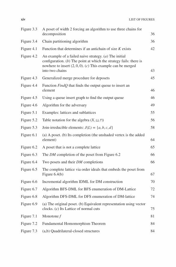
Figure 3.3 A poset of width 2 forcing an algorithm to use three chains fordecomposition 36
Figure 3.4 Chain partitioning algorithm 36
Figure 4.1 Function that determines if an antichain of size K exists 42
Figure 4.2 An example of a failed naive strategy. (a) The initialconfiguration. (b) The point at which the strategy fails: there isnowhere to insert (2, 0, 0). (c) This example can be mergedinto two chains 43
Figure 4.3 Generalized merge procedure for deposets 45
Figure 4.4 Function FindQ that finds the output queue to insert anelement 46
Figure 4.5 Using a queue insert graph to find the output queue 46
Figure 4.6 Algorithm for the adversary 49
Figure 5.1 Examples: lattices and sublattices 55
Figure 5.2 Table notation for the algebra (X, ⊔, ⊓) 56
Figure 5.3 Join-irreducible elements: J(L) = {a, b, c, d} 58
Figure 6.1 (a) A poset. (b) Its completion (the unshaded vertex is the addedelement) 64
Figure 6.2 A poset that is not a complete lattice 65
Figure 6.3 The DM completion of the poset from Figure 6.2 66
Figure 6.4 Two posets and their DM completions 66
Figure 6.5 The complete lattice via order ideals that embeds the poset fromFigure 6.4(b) 67
Figure 6.6 Incremental algorithm IDML for DM construction 70
Figure 6.7 Algorithm BFS-DML for BFS enumeration of DM-Lattice 72
Figure 6.8 Algorithm DFS-DML for DFS enumeration of DM-lattice 74
Figure 6.9 (a) The original poset. (b) Equivalent representation using vectorclocks. (c) Its Lattice of normal cuts 75
Figure 7.1 Monotone f 81
Figure 7.2 Fundamental Homomorphism Theorem 84
Figure 7.3 (a,b) Quadrilateral-closed structures 84

LIST OF FIGURES xv
Figure 7.4 Simple reduction of state graph does not preserve path basedformulas 86
Figure 7.5 (a,b) Proof of Lemma 7.13 88
Figure 7.6 Proof of Lemma 7.14 89
Figure 8.1 Proof of Theorem 8.5 93
Figure 8.2 Theorem 8.9 96
Figure 8.3 (a) A ranked poset, (b) A poset that is not ranked, (c) A rankedand graded poset, and (d) A ranked and graded lattice 97
Figure 9.1 Diamond M3—a nondistributive lattice 100
Figure 9.2 A lattice L, its set of join-irreducibles J(L), and their idealsLI(J(L)) 103
Figure 9.3 A lattice with the “N-poset” as the set of join-irreducibles 103
Figure 9.4 (a) Poset of Join- (“j”) and meet- (“m”) irreducible elements areisomorphic; (b) Irreducibles in a nondistributive lattice 104
Figure 10.1 (a) P: A partial order. (b) The lattice of ideals. (c) The directedgraph P′ 108
Figure 10.2 (a) A directed graph and (b) the lattice of its nontrivial ideals 109
Figure 10.3 (a) The poset or directed graph for generating subsets of Xof size k. (b) The ideal denoting the subset {1, 3, 4} 109
Figure 10.4 Graphs and slices for generating subsets of X when |X| = 4 110
Figure 10.5 An efficient algorithm to detect a linear predicate 113
Figure 10.6 An efficient algorithm to compute the slice for a predicate B 116
Figure 10.7 An efficient algorithm to compute the slice for a linearpredicate B 117
Figure 11.1 Graphs and slices for generating subsets of X when |X| = 4 122
Figure 11.2 Slice for the predicate “does not contain consecutive numbers” 123
Figure 11.3 Ferrer’s diagram for the integer partition (4, 2, 1) for 7 124
Figure 11.4 An Application of Ferrer’s diagram 124
Figure 11.5 Young’s lattice for (3, 3, 3) 125
Figure 11.6 The poset corresponding to Ferrer’s diagram of (3, 3, 3) 125
Figure 11.7 Slice for 𝛿2 = 2 126

xvi LIST OF FIGURES
Figure 11.8 Slice for “distinct parts.” 127
Figure 11.9 Poset T(5). 128
Figure 11.10 Slice for subsets of permutations 129
Figure 12.1 A poset that is a ranking 132
Figure 12.2 Examples of weak orders (or rankings.) 132
Figure 12.3 A poset and its normal ranking extension 133
Figure 12.4 Mapping elements of poset to interval order 136
Figure 13.1 Example series and parallel compositions. (a–c) Posets.(d) Result of P2 + P3. (e) Result of P1 ∗ (P2 + P3) 140
Figure 13.2 (a) An SP tree for the poset in Figure 13.1(e). (b) Theconjugate SP tree. (c) The conjugate poset 141
Figure 13.3 (a) A two-dimensional poset. (b) Its comparability graph G.(c) GC. (d) A valid conjugate for the original poset 142
Figure 13.4 The poset S3 142
Figure 13.5 (a) is a non-separating linear extension of the partial order (b),when at least one of the dotted edges holds 143
Figure 13.6 A two-dimensional Poset P = (X,≤P) 144
Figure 13.7 Conjugate Q = L1 ∩ L2−1 of the poset P 144
Figure 13.8 The order imposed by ≤P ∪ ≤Q 145
Figure 13.9 A partial order P that has a nonseparating linear extension 146
Figure 14.1 (a) A computation. (b) Its lattice of consistent global states. (c)Traversals of the lattice 150
Figure 14.2 BFS enumeration of CGS 152
Figure 14.3 A vector clock based BFS enumeration of CGS 153
Figure 14.4 A vector clock based DFS enumeration of CGS 155
Figure 14.5 An algorithm for lexical traversal of all ideals of a poset with anychain partition 158
Figure 14.6 L(3, 3) with example of an ideal 159
Figure 14.7 (a) Poset L(n,m) with uniflow partition. (b) L(3, 3) with anexample of an ideal mapped to the subset {1, 3, 4} 161
LIST OF FIGURES xvii
Figure 14.8 (a) Poset D(n,m) with uniflow partition (b) D(3, 3) with exampleof an ideal 161
Figure 14.9 (a) Chain partition of a Poset that is not uniflow. (b) Uniflowchain partition of the same poset 162
Figure 14.10 An algorithm for traversal of product space in lex order 164
Figure 14.11 Posets for generating subsets of X 165
Figure 14.12 (a) Poset C(5) with a uniflow partition (b) Poset T(5)with a uniflow partition 166
Figure 14.13 An algorithm for traversal of all subsets of [n] of size m in lexorder 166
Figure 14.14 (a) A Ferrer’s diagram. (b) A poset for generating Young’slattice 167
Figure 14.15 An algorithm for traversal of all integer partitions in Y𝜆 in lexorder 167
Figure 14.16 An algorithm for traversal of a level set in lexical order 169
Figure 14.17 (a) Poset NL(n,m) with a negative uniflow partition. (b) NL(3, 3)with example of an ideal 169
Figure 14.18 An algorithm to find the lexically smallest ideal at level rgreater than G 170
Figure 14.19 An Algorithm to find the next bigger ideal in a level set 171
Figure 15.1 (a) The original poset. (b) Its lattice of ideals (consistent cuts).(c) Its lattice of maximal antichains 160
Figure 15.2 (a) The original poset. (b) Its lattice of maximal ideals.(c) Its lattice of maximal antichains. (d) Its lattice of strictideals 162
Figure 15.3 The algorithm ILMA for construction of lattice of maximalantichains 164
Figure 15.4 The algorithm OLMA for construction of lattice of strictideals 166
Figure 15.5 Algorithm DFS-MA for DFS enumeration of lattice of maximalantichains 168
Figure 15.6 An algorithm for traversal of closed sets in lex order 172
Figure 16.1 An example of a realizer 178
Figure 16.2 Standard example S5 179

xviii LIST OF FIGURES
Figure 16.3 Example of a critical pair: (a1, b1) 183
Figure 16.4 A poset with a chain realizer and a string realizer 185
Figure 16.5 Encoding an infinite poset with strings 185
Figure 16.6 An example of converting a string realizer to a chain realizer 188
Figure 16.7 A bipartite poset 190
Figure 16.8 String realizer for the bipartite poset in Figure 16.7 190
Figure 16.9 Encoding for the bipartite poset in Figure 16.7 192
Figure 16.10 Another Encoding for the bipartite poset in Figure 16.7 192
Figure 16.11 An example of a poset with rectangular dimension two 194
Figure 16.12 An example of decomposing a poset into series-parallel posets 196

NOMENCLATURE
⊥ Bottom element of the latticeJ(P) Set of join-irreducible elements of a poset PLI Lattice of idealsLDM Lattice of normal cutsLMA Lattice of maximal antichainsLWA Lattice of width antichainsM(P) Set of meet-irreducible elements of a poset P⊓ Meet⊔ Join⊤ Top element of the latticen A poset consisting of a single chain of length na ∼P b a is comparable to b in PAl Set of lower bounds of AAu Set of upper bounds of AD(x) Set of elements less than xD[x] Set of elements less than or equal to xDM(P) Dedekind–MacNeille Completion of PPd Dual poset of PU(x) Set of elements greater than xU[x] Set of elements greater than or equal to x

PREFACE
As many books exist on lattice theory, I must justify writing another book on thesubject. This book is written from the perspective of a computer scientist ratherthan a mathematician. In many instances, a mathematician may be satisfied with anonconstructive existential proof, but a computer scientist is interested not only inconstruction but also in the computational complexity of the construction. I haveattempted to give “algorithmic” proofs of theorems whenever possible.
This book is also written for the sake of students rather than a practicing math-ematician. In many instances, a student needs to learn the heuristics that guide theproof, besides the proof itself. It is not sufficient just to learn an important theorem.One must also learn ways to extend and analyze a theorem. I have also made an effortto include exercises with each chapter. A mathematical subject can only be learnedby solving problems related to that subject.
I would like to thank the students at the University of Texas at Austin, who tookmy course on lattice theory. I also thank my co-authors for various papers related tolattice theory and applications in distributed computing: Anurag Agarwal, ArindamChakraborty, Yen-Jung Chang, Craig Chase, Himanshu Chauhan, Selma Ikiz, Rat-nesh Kumar, Neeraj Mittal, Sujatha Kashyap, Vinit Ogale, Alper Sen, AlexanderTomlinson, and Brian Waldecker. I owe special thanks to Bharath Balasubraman-ina, Vinit Ogale, Omer Shakil, Alper Sen, and Roopsha Samanta who reviewed partsof the book.
I thank the Department of Electrical and Computer Engineering at The Universityof Texas at Austin, where I was given the opportunity to develop and teach a courseon lattice theory.
I have also been supported in part by many grants from the National Science Foun-dation. This book would not have been possible without that support.

xxii PREFACE
Finally, I thank my parents, wife, and children. Without their love and support,this book would not have been even conceived.
The list of known errors and the supplementary material for the book will be main-tained on my homepage:
http://www.ece.utexas.edu/~garg
Vijay K. GargAustin, Texas.

BIBLIOGRAPHY
[AG05] A. Agarwal and V. K. Garg. Efficient dependency tracking for relevant events inshared-memory systems. In M. K. Aguilera and J. Aspnes, editors, Proceedings of theTwenty-Fourth Annual ACM Symposium on Principles of Distributed Computing, PODC2005, Las Vegas, NV, July 17-20, 2005, pages 19–28. ACM, 2005.
[AGO10] A. Agarwal, V. K. Garg, and V. A. Ogale. Modeling and analyzing periodicdistributed computations. In S. Dolev, J. A. Cobb, M. J. Fischer, and M. Yung, editors,Stabilization, Safety, and Security of Distributed Systems - 12th International Symposium,SSS 2010, New York, NY, September 20-22, 2010. Proceedings, volume 6366 of LectureNotes in Computer Science, pages 191–205. Springer, 2010.
[AV01] S. Alagar and S. Venkatesan. Techniques to tackle state explosion in global predicatedetection. IEEE Transactions on Software Engineering, 27(8):704–714, 2001.
[Bir40] G. Birkhoff. Lattice Theory. Providence, RI, 1940. First edition.
[Bir48] G. Birkhoff. Lattice Theory. Providence, RI, 1948. Second edition.
[Bir67] G. Birkhoff. Lattice Theory. Providence, RI, 1967. Third edition.
[Bog93] K. P. Bogart. An obvious proof of fishburn’s interval order theorem. DiscreteMathematics, 118(1):21–23, 1993.
[BFK+12] B. Bosek, S. Felsner, K. Kloch, T. Krawczyk, G. Matecki, and P. Micek. On-linechain partitions of orders: a survey. Order, 29:49–73, 2012. DOI: 10.1007/s11083-011-9197-1.
[CLM12] N. Caspard, B. Leclerc, and B. Monjardet. Finite Ordered Sets: Concepts, Resultsand Uses, volume 144. Cambridge University Press, 2012.
Introduction to Lattice Theory with Computer Science Applications, First Edition. Vijay K. Garg.© 2015 John Wiley & Sons, Inc. Published 2015 by John Wiley & Sons, Inc.
230 BIBLIOGRAPHY
[CG06] A. Chakraborty and V. K. Garg. On reducing the global state graph for verificationof distributed computations. In International Workshop on Microprocessor Test andVerification (MTV’06), Austin, TX, December 2006.
[CG95] C. Chase and V. K. Garg. On techniques and their limitations for the global predi-cate detection problem. In Proceedings of the Workshop on Distributed Algorithms, pages303–317, France, September 1995.
[CG98] C. M. Chase and V. K. Garg. Detection of global predicates: techniques and theirlimitations. Distributed Computing, 11(4):191–201, 1998.
[CM91] R. Cooper and K. Marzullo. Consistent detection of global predicates. In Proceedingsof the Workshop on Parallel and Distributed Debuyyiny, pages 163–173, Santa Cruz, CA,May 1991.
[CLRS01] T. H. Cormen, C. E. Leiserson, R. L. Rivest, and C. Stein. Introduction to Algo-rithms. The MIT Press and McGraw-Hill, 2001. Second edition.
[DP90] B. A. Davey and H. A. Priestley. Introduction to Lattices and Order. CambridgeUniversity Press, Cambridge, UK, 1990.
[DS90] E. W. Dijkstra and C. S. Scholten. Predicate Calculus and Program Semantics.Springer-Verlag New York Inc., New York, 1990.
[Dil50] R. P. Dilworth. A decomposition theorem for partially ordered sets. Annals of Math-ematics, 51:161–166, 1950.
[DM41] B. Dushnik and E. Miller. Partially ordered sets. American Journal of Mathematics,63:600–610, 1941.
[Ege31] E. Egervary. On combinatorial properties of matrices. Matematikai Lapok, 38:16–28,1931.
[ER03] S. Effler and F. Ruskey. A CAT algorithm for generating permutations with a fixednumber of inversions. Information Processing Letters, 86(2), 107–112, (2003).
[FLST86] U. Faigle, L. Lovász, R. Schrader, and Gy. Turán. Searching in trees, series-paralleland interval orders. SIAM Journal on Computing, 15(4):1075–1084, 1986.
[Fel97] S. Felsner. On-line chain paritions of orders. Theoretical Computer Science, 175:283–292, 1997.
[Fid89] C. J. Fidge. Partial orders for parallel debugging. Proceedings of the ACM SIG-PLAN/SIGOPS Workshop on Parallel and Distributed Debugging, (ACM SIGPLANNotices), 24(1):183–194, 1989.
[Fis85] P. C. Fishburn. Interval Orders and Interval Graphs. John Wiley and Sons, 1985.
[FJN96] R. Freese, J. Jaroslav, and J. B. Nation. Free Lattices. American MathematicalSociety, 1996.
[Ful56] D. R. Fulkerson. Note on dilworth’s decomposition theorem for partially ordered sets.Proceedings of the American Mathematical Society, 7(4):701–702, 1956.
[Gal94] F. Galvin. A proof of dilworth’s chain decomposition theorem. American Mathemat-ical Monthly, 101(4):352–353, 1994.
[GR91] B. Ganter and K. Reuter. Finding all closed sets: a general approach. Order,8(3):283–290, 1991.
[Gar92] V. K. Garg. An algebraic approach to modeling probabilistic discrete event sys-tems. In Decision and Control, 1992, Proceedings of the 31st IEEE Conference on, pages2348–2353. IEEE, 1992.

BIBLIOGRAPHY 231
[Gar03] V. K. Garg. Enumerating global states of a distributed computation. In Interna-tional Conference on Parallel and Distributed Computing and Systems, pages 134–139,November 2003.
[Gar06] V. K. Garg. Algorithmic combinatorics based on slicing posets. Theoretical ComputerScience, 359(1-3):200–213, 2006.
[Gar12] V. K. Garg. Lattice completion algorithms for distributed computations. In Proceed-ings of Principles of Distributed Systems, 16th International Conference, OPODIS 2012,Rome, Italy, December 18-20, 2012. pages 166–180, December 2012.
[Gar13] V. K. Garg. Maximal antichain lattice algorithms for distributed computations.In D. Frey, M. Raynal, S. Sarkar, R. K. Shyamasundar, and P. Sinha, editors, ICDCN,volume 7730 of Lecture Notes in Computer Science, pages 240–254. Springer, 2013.
[Gar14] V. K. Garg. Lexical enumeration of combinatorial structures by enumerating orderideals. Technical report, University of Texas at Austin, Dept. of Electrical and ComputerEngineering, Austin, TX, 2014.
[GM01] V. K. Garg and N. Mittal. On slicing a distributed computation. In 21st InternationalConference on Distributed Computing Systems (ICDCS’ 01), pages 322–329, Washington -Brussels - Tokyo, April 2001. IEEE.
[GS01] V. K. Garg and C. Skawratananond. String realizers of posets with applications todistributed computing. In 20th Annual ACM Symposium on Principles of Distributed Com-puting (PODC-00), pages 72–80. ACM, August 2001.
[Grä71] G. Grätzer. Lattice Theory. W.H. Freeman and Company, San Francisco, CA, 1971.
[Grä03] G. Grätzer. General Lattice Theory. Birkhäuser, Basel, 2003.
[HM84] J.Y. Halpern and Y. Moses. Knowledge and common knowledge in a distributed envi-ronment. In Proceedings of the ACM Symposium on Principles of Distributed Computing,pages 50–61, Vancouver, BC, 1984.
[Hir55] T. Hiraguchi. On the dimension of orders. Science Reports of Kanazawa University,4:1–20, 1955.
[HK71] J. E. Hopcroft and R. M. Karp. A n5∕2 algorithm for maximum matchings in bipartite.In Switching and Automata Theory, 1971, 12th Annual Symposium on, pages 122 –125,October 1971.
[IG06] S. Ikiz and V. K. Garg. Efficient incremental optimal chain partition of distributedprogram traces. In ICDCS, page 18. IEEE Computer Society, 2006.
[JRJ94] G.-V. Jourdan, J.-X. Rampon, and C. Jard. Computing on-line the lattice of maximalantichains of posets. Order, 11:197–210, 1994. DOI: 10.1007/BF02115811.
[Kie81] H. A. Kierstead. Recursive colorings of highly recursive graphs. Canadian Journalof Mathematics, 33(6):1279–1290, 1981.
[Knu98] D. E. Knuth. Sorting and searching, volume 3 of The Art of Computer Programming.Addison-Wesley, Reading, MA, Second edition, 1998.
[Koh83] K. M. Koh. On the lattice of maximum-sized antichains of a finite poset. AlgebraUniversalis, 17(1):73–86, 1983.
[Kon31] D. Konig. Graphen und matrizen. Matematikai és Fizikai Lapok, 38:116–119, 1931.
[Lam78] L. Lamport. Time, clocks, and the ordering of events in a distributed system.Communications of the ACM, 21(7):558–565, 1978.
232 BIBLIOGRAPHY
[LNS82] J.-L. Lassez, V. L. Nguyen, and E. A. Sonenberg. Fixed point theorems andsemantics: a folk tale. Information Processing Letters, 14(3):112–116, 1982.
[Mat89] F. Mattern. Virtual time and global states of distributed systems. In Proceedings ofthe International Workshop on Parallel and Distributed Algorithms, pages 215–226, 1989.
[Mir71] L. Mirsky. A dual of dilworth’s decomposition theorem. American MathematicalMonthly, 78(8):876–877, 1971.
[MG01a] N. Mittal and V. K. Garg. On detecting global predicates in distributed computations.In 21st International Conference on Distributed Computing Systems (ICDCS’ 01), pages3–10, Washington - Brussels - Tokyo, April 2001. IEEE.
[MG01b] N. Mittal and V. K. Garg. Slicing a distributed computation: Techniques and theory.In 5th International Symposium on DIStributed Computing (DISC’01), October 2001.
[MG04] N. Mittal and V. K. Garg. Rectangles are better than chains for encoding partiallyordered sets. Technical report, University of Texas at Austin, Dept. of Electrical andComputer Engineering, Austin, TX, September 2004.
[MSG07] N. Mittal, A. Sen, and V. K. Garg. Solving computation slicing using predicatedetection. IEEE Transactions on Parallel and Distributed Systems, 18(12):1700–1713,2007.
[Moh89] R. H. Mohring. Computationally tractable classes of ordered sets. Algorithms andOrder, pages 105–192. Kluwer Academic Publishers, Dordrecht, 1989.
[NR99] L. Nourine and O. Raynaud. A fast algorithm for building lattices. Information Pro-cessing Letters, 71(5-6):199–204, 1999.
[NR02] L. Nourine and O. Raynaud. A fast incremental algorithm for building lattices. Journalof Experimental & Theoretical Artificial Intelligence, 14(2-3):217–227, 2002.
[RR79] I. Rabinovitch and I. Rival. The rank of a distributive lattice. Discrete Mathematics,25(3):275–279, 1979.
[RT10] O. Raynaud and E. Thierry. The complexity of embedding orders into small productsof chains. Order, 27:365–381, 2010.
[Rea02] N. Reading. Order dimension, strong bruhat order and lattice properties of posets.Order, 19:73–100, 2002.
[Reu91] K. Reuter. The jump number and the lattice of maximal antichains. Discrete Mathe-matics, 88(2â “3):289–307, 1991.
[Rom08] S. Roman. Lattices and Ordered Sets. Springer, 2008.
[Spi85] J. Spinrad. On comparability and permutation graphs. SIAM Journal on Computing,14(3):658–670, 1985.
[SW86] D. Stanton and D. White. Constructive Combinatorics. Springer-Verlag, 1986.
[Ste84] G. Steiner. Single machine scheduling with precedence constraints of dimension 2.Mathematics of Operations Research, 9:248–259, 1984.
[Szp37] E. Szpilrajn. La dimension et la mesure. Fundamenta Mathematicae, 28:81–89, 1937.
[Tar55] A. Tarski. A lattice-theoretic fixed point theorem and its applications. Pacific Journalof Mathematics, 5:285–309, 1955.
[TG97] A. I. Tomlinson and V. K. Garg. Monitoring functions on global states of distributedprograms. Journal for Parallel and Distributed Computing, 1997. a preliminary versionappeared in Proceedings of the ACM Workshop on Parallel and Distributed Debugging,San Diego, CA, May 1993, pp.21–31.

BIBLIOGRAPHY 233
[Tro92] W. T. Trotter. Combinatorics and Partially Ordered Sets: Dimension Theory. TheJohns Hopkins University Press, 1992.
[vLW92] J. H. van Lint and R. M. Wilson. A Course in Combinatorics. Cambridge UniversityPress, 1992.
[Wes04] D. B. West. Order and Optimization. 2004. pre-release version.

1INTRODUCTION
1.1 INTRODUCTION
Partial order and lattice theory play an important role in many disciplines of computerscience and engineering. For example, they have applications in distributed comput-ing (vector clocks and global predicate detection), concurrency theory (pomsets andoccurrence nets), programming language semantics (fixed-point semantics), and datamining (concept analysis). They are also useful in other disciplines of mathematicssuch as combinatorics, number theory, and group theory.
This book differs from earlier books written on the subject in two aspects. First,this book takes a computational perspective—the emphasis is on algorithms and theircomplexity. While mathematicians generally identify necessary and sufficient condi-tions to characterize a property, this book focuses on efficient algorithms to test theproperty. As a result of this bias, much of the book concerns itself only with finitesets. Second, existing books do not dwell on applications of lattice theory. This booktreats applications at par with the theory. In particular, I have given applications oflattice theory to distributed computing and combinatorics.
This chapter covers the basic definitions of partial orders.
Introduction to Lattice Theory with Computer Science Applications, First Edition. Vijay K. Garg.© 2015 John Wiley & Sons, Inc. Published 2015 by John Wiley & Sons, Inc.

2 INTRODUCTION
1.2 RELATIONS
A partial order is simply a relation with certain properties. A relation R over any setX is a subset of X × X. For example, let
X = {a, b, c}.
Then, one possible relation is
R = {(a, c), (a, a), (b, c), (c, a)}.
It is sometimes useful to visualize a relation as a graph on the vertex set X suchthat there is a directed edge from x to y iff (x, y) ∈ R. The graph corresponding to therelation R in the previous example is shown in Figure 1.1.
A relation is reflexive if for each x ∈ X, (x, x) ∈ R, i.e., each element of X is relatedto itself. In terms of a graph, this means that there is a self-loop on each node. IfX is the set of natural numbers, , then “x divides y” is a reflexive relation. R isirreflexive if for each x ∈ X, (x, x) ∉ R. In terms of a graph, this means that there areno self-loops. An example on the set of natural numbers, , is the relation “x lessthan y.” Note that a relation may be neither reflexive nor irreflexive.
A relation R is symmetric if for all x, y ∈ X, (x, y) ∈ R implies (y, x) ∈ R. Anexample of a symmetric relation on is
R = {(x, y) | x mod 5 = y mod 5}. (1.1)
A symmetric relation can be represented using an undirected graph. R is antisym-metric if for all x, y ∈ X, (x, y) ∈ R and (y, x) ∈ R implies x = y. For example, therelation less than or equal to defined on is anti-symmetric. A relation R is asym-metric if for all x, y ∈ X, (x, y) ∈ R implies (y, x) ∉ R. The relation less than on isasymmetric. Note that an asymmetric relation is always irreflexive.
A relation R is transitive if for all x, y, z ∈ X, (x, y) ∈ R and (y, z) ∈ R implies(x, z) ∈ R. The relations less than and equal to on are transitive.
c
ba
Figure 1.1 The graph of a relation.

PARTIAL ORDERS 3
A relation R is an equivalence relation if it is reflexive, symmetric, and transitive.When R is an equivalence relation, we use x ≡R y (or simply x ≡ y when R is clearfrom the context) to denote that (x, y) ∈ R. Furthermore, for each x ∈ X, we use [x]R,called the equivalence class of x, to denote the set of all y ∈ X such that y ≡R x. Itcan be seen that the set of all such equivalence classes forms a partition of X. Therelation on defined in (1.1) is an example of an equivalence relation. It partitionsthe set of natural numbers into five equivalence classes.
Given any relation R on a set X, we define its irreflexive transitive closure,denoted by R+, as follows. For all x, y ∈ X ∶ (x, y) ∈ R+ iff there exists a sequencex0, x1, ..., xj, j ≥ 1 with x0 = x and xj = y such that
∀i ∶ 0 ≤ i < j ∶ (xi, xi+1) ∈ R.
Thus (x, y) ∈ R+, iff there is a nonempty path from x to y in the graph of the relation R.We define the reflexive transitive closure, denoted by R∗, as
R∗ = R+ ∪ {(x, x) | x ∈ X}.
Thus (x, y) ∈ R∗ iff y is reachable from x by taking a path with zero or more edges inthe graph of the relation R.
1.3 PARTIAL ORDERS
A relation R is a reflexive partial order (or, a nonstrict partial order) if it is reflex-ive, antisymmetric, and transitive. The divides relation on the set of natural numbersis a reflexive partial order. A relation R is an irreflexive partial order, or a strictpartial order if it is irreflexive and transitive. The less than relation on the set ofnatural numbers is an irreflexive partial order. When R is a reflexive partial order, weuse x ≤R y (or simply x ≤ y when R is clear from the context) to denote that (x, y) ∈ R.A reflexive partially ordered set, poset for short, is denoted by (X,≤). When R is anirreflexive partial order, we use x <R y (or simply x < y when R is clear from the con-text) to denote that (x, y) ∈ R. The set X together with the partial order is denoted by(X, <). We use P = (X, <) to denote a irreflexive poset defined on X.
The two versions of partial orders—reflexive and irreflexive—are essentially thesame. Given an irreflexive partial order, we can define x ≤ y as x < y or x = y, whichgives us a reflexive partial order. Similarly, given a reflexive partial order (X,≤), wecan define an irreflexive partial order (X, <) by defining x < y as x ≤ y and x ≠ y.
A relation is a total order if R is a partial order and for all distinct x, y ∈ X, either(x, y) ∈ R or (y, x) ∈ R. The natural order on the set of integers is a total order, but thedivides relation is only a partial order.
Finite posets are often depicted graphically using Hasse diagrams. To defineHasse diagrams, we first define a relation covers as follows. For any two elementsx, y ∈ X, y covers x if x < y and ∀z ∈ X ∶ x ≤ z < y implies z = x. In other words, ify covers x then there should not be any element z with x < z < y. We use x <c y to

4 INTRODUCTION
r
q
p
s
Figure 1.2 Hasse diagram.
denote that y covers x (or x is covered by y). We also say that y is an upper cover ofx and x is a lower cover of y. A Hasse diagram of a poset is a graph with the propertythat there is an edge from x to y iff x <c y. Furthermore, when drawing the graph on aEuclidean plane, x is drawn lower than y when y covers x. This allows us to suppressthe directional arrows in the edges. For example, consider the following poset (X,≤),
Xdef= {p, q, r, s}; ≤
def= {(p, q), (q, r), (p, r), (p, s)}. (1.2)
The corresponding Hasse diagram is shown in Figure 1.2. Note that we will some-times use directed edges in Hasse diagrams if the context demands it. In general, inthis book, we switch between the directed graph and undirected graph representationsof Hasse diagrams.
Given a poset (X,≤X) a subposet is simply a poset (Y ,≤Y ), where Y ⊆ X, and
∀x, y ∈ Y ∶ x ≤Y ydef= x ≤X y.
Let x, y ∈ X with x ≠ y. If either x < y or y < x, we say x and y are comparable. Onthe other hand, if neither x < y nor x > y, then we say x and y are incomparable andwrite x||y. A poset (Y ,≤) (or a subposet (Y ,≤) of (X,≤)) is called a chain if everydistinct pair of elements from Y is comparable. Similarly, we call a poset an antichainif every distinct pair of elements from Y is incomparable. For example, for the posetrepresented in Figure 1.2, {p, q, r} is a chain, and {q, s} is an antichain.
A chain C of a poset (X,≤) is a longest chain if no other chain contains moreelements than C. We use a similar definition for the largest antichain. The heightof the poset is the number of elements in a longest chain, and the width of the posetis the number of elements in a largest antichain. For example, the poset in Figure 1.2has height equal to 3 (the longest chain is {p, q, r}) and width equal to 2 (a largestantichain is {q, s}).

JOIN AND MEET OPERATIONS 5
b
d
b c
d
a
c
b
a
a
fe
e
Figure 1.3 Only the first two posets are lattices.
Generalizing the notation for intervals on the real-line, we define an interval [x, y]in a poset (X,≤) as
{z | x ≤ z ≤ y}.
The meanings of (x, y), [x, y) and (x, y] are similar. A poset is locally finite if allintervals are finite. Most posets in this book will be locally finite if not finite.
A poset is well-founded iff it has no infinite decreasing chain. The set of natu-ral numbers under the usual ≤ relation is well-founded but the set of integers is notwell-founded.
Poset Q = (X,≤Q) extends the poset P = (X,≤P) if
∀x, y ∈ X ∶ x ≤P y ⇒ x ≤Q y.
If Q is a total order, then we call Q a linear extension of P. For example, for theposet P = (X,≤) defined in Figure 1.2, a possible linear extension Q is
Xdef= {p, q, r, s}; ≤Q
def= {(p, q), (q, r), (p, r), (p, s), (q, s), (r, s)}.
We now give some special posets that will be used as examples in the book.
• n denotes a poset which is a chain of length n. The second poset in Figure 1.3is 2.
• We use An to denote the poset of n incomparable elements.
1.4 JOIN AND MEET OPERATIONS
We now define two operators on subsets of the set X—meet and join. The opera-tor meet is also called infimum (or inf). Similarly, the operator join is also calledsupremum (or sup).
6 INTRODUCTION
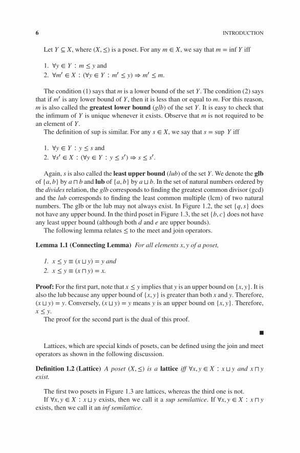
Let Y ⊆ X, where (X,≤) is a poset. For any m ∈ X, we say that m = inf Y iff
1. ∀y ∈ Y ∶ m ≤ y and
2. ∀m′ ∈ X ∶ (∀y ∈ Y ∶ m′ ≤ y) ⇒ m′ ≤ m.
The condition (1) says that m is a lower bound of the set Y . The condition (2) saysthat if m′ is any lower bound of Y , then it is less than or equal to m. For this reason,m is also called the greatest lower bound (glb) of the set Y . It is easy to check thatthe infimum of Y is unique whenever it exists. Observe that m is not required to bean element of Y .
The definition of sup is similar. For any s ∈ X, we say that s = sup Y iff
1. ∀y ∈ Y ∶ y ≤ s and
2. ∀s′ ∈ X ∶ (∀y ∈ Y ∶ y ≤ s′) ⇒ s ≤ s′.
Again, s is also called the least upper bound (lub) of the set Y . We denote the glbof {a, b} by a ⊓ b and lub of {a, b} by a ⊔ b. In the set of natural numbers ordered bythe divides relation, the glb corresponds to finding the greatest common divisor (gcd)and the lub corresponds to finding the least common multiple (lcm) of two naturalnumbers. The glb or the lub may not always exist. In Figure 1.2, the set {q, s} doesnot have any upper bound. In the third poset in Figure 1.3, the set {b, c} does not haveany least upper bound (although both d and e are upper bounds).
The following lemma relates ≤ to the meet and join operators.
Lemma 1.1 (Connecting Lemma) For all elements x, y of a poset,
1. x ≤ y ≡ (x ⊔ y) = y and
2. x ≤ y ≡ (x ⊓ y) = x.
Proof: For the first part, note that x ≤ y implies that y is an upper bound on {x, y}. It isalso the lub because any upper bound of {x, y} is greater than both x and y. Therefore,(x ⊔ y) = y. Conversely, (x ⊔ y) = y means y is an upper bound on {x, y}. Therefore,x ≤ y.
The proof for the second part is the dual of this proof.
Lattices, which are special kinds of posets, can be defined using the join and meetoperators as shown in the following discussion.
Definition 1.2 (Lattice) A poset (X,≤) is a lattice iff ∀x, y ∈ X ∶ x ⊔ y and x ⊓ yexist.
The first two posets in Figure 1.3 are lattices, whereas the third one is not.If ∀x, y ∈ X ∶ x ⊔ y exists, then we call it a sup semilattice. If ∀x, y ∈ X ∶ x ⊓ y
exists, then we call it an inf semilattice.

OPERATIONS ON POSETS 7
(a) (b)0
b
c
a
1
0
a b c
1
Figure 1.4 (a) Pentagon(N5) and (b) diamond(M3).
In our definition of lattice, we have required existence of lub’s and glb’s for setsof size two. This is equivalent to the requirement of existence of lub’s and glb’s forsets of finite size by using induction. A poset may be a lattice, but it may have setsof infinite size for which lub/glb may not exist. A simple example is that of the setof natural numbers. There is no lub of set of even numbers, even though glb andlub exist as min and max for any finite set. Another example is the set of rationalnumbers. For a finite subset of rational numbers, we can easily determine lubs(andglbs). However, consider the set {x | x ≤
√2}. The lub of this set is
√2, which is
not a rational number. A lattice for which any set has lub and glb defined is called acomplete lattice. An example of a complete lattice is the set of real numbers extendedwith +∞ and −∞.
Definition 1.3 (Distributive Lattice) A lattice L is distributive if
∀a, b, c ∈ L ∶ a ⊓ (b ⊔ c) = (a ⊓ b) ⊔ (a ⊓ c).
It is easy to verify that the above-mentioned condition is equivalent to
∀a, b, c ∈ L ∶ a ⊔ (b ⊓ c) = (a ⊔ b) ⊓ (a ⊔ c).
Thus, in a distributive lattice, ⊔ and ⊓ operators distribute over each other.Any power-set lattice is distributive. The lattice of natural numbers with ≤ defined
as the relation divides is also distributive. Some examples of nondistributive latticesare diamond (M3) and pentagon (N5) shown in Figure 1.4.
1.5 OPERATIONS ON POSETS
Given any set of structures, it is useful to consider ways of composing them to obtainnew structures.

8 INTRODUCTION
1
00
2
(1,1)
(1,0)
(1,2)
1
(0,1)
(0,0)
(0,2)
Figure 1.5 Cross product of posets.
Definition 1.4 (Disjoint Sum) Given two posets P and Q, their disjoint sum,denoted by P + Q, is defined as follows. Given any two elements x and y in P + Q,x ≤ y iff
(1) both x and y belong to P and x ≤ y in P or(2) both x and y belong to Q and x ≤ y in Q.
The Hasse diagram of the disjoint sum of P and Q can be computed by simply placingthe Hasse diagram of P next to Q.
Definition 1.5 (Cross Product of Posets) Given two posets P and Q, the cross prod-uct denoted by P × Q is defined as
(P × Q,≤P×Q)
where(p1, q1) ≤ (p2, q2)
def= (p1 ≤P p2) ∧ (q1 ≤Q q2).
See Figure 1.5 for an example. The definition can be extended to an arbitrary indexingset.
Definition 1.6 (Linear Sum) Given two posets P and Q, the linear sum (or ordinalsum) denoted by P ⊕ Q is defined as
x ≤P⊕Q y iff (x ≤P y) ∨ (x ≤Q y) ∨ [(x ∈ P) ∧ (y ∈ Q)].
1.6 IDEALS AND FILTERS
Let (X,≤) be any poset. We call a subset Y ⊆ X a down-set if
∀y, z ∈ X ∶ z ∈ Y ∧ y ≤ z ⇒ y ∈ Y .
Down-sets are also called order ideals. It is easy to see that for any x, D[x] definedbelow is an order ideal. Such order ideals are called principal order ideals,
D[x] = {y ∈ X | y ≤ x}.

SPECIAL ELEMENTS IN POSETS 9
For example, in Figure 1.2, D[r] = {p, q, r}. Similarly, we call Y ⊆ X an up-set if
y ∈ Y ∧ y ≤ z ⇒ z ∈ Y .
Up-sets are also called order filters. We also use the notation below to denote prin-cipal order filters
U[x] = {y ∈ X|x ≤ y}.
In Figure 1.2, U[p] = {p, q, r, s}.
The following lemma provides a convenient relationship between principal orderfilters and other operators defined earlier.
Lemma 1.7 1. x ≤ y ≡ U[y] ⊆ U[x]2. x = sup Y ≡ U[x] = ∩y∈YU[y].
Proof: Left as an exercise.
In some applications, the following notation is also useful:
U(x) = {y ∈ X|x < y}
D(x) = {y ∈ X|y < x}.
We will call U(x) the upper-holdings of x, and D(x), the lower-holdings of x.We can extend the definitions of D[x],D(x),U[x],U(x) to sets of elements, A. Forexample,
U[A] = {y ∈ X|∃x ∈ A ∶ x ≤ y}.
1.7 SPECIAL ELEMENTS IN POSETS
We define some special elements of posets such as bottom and top elements, andminimal and maximal elements.
Definition 1.8 (Bottom Element) An element x is a bottom element or a minimumelement of a poset P if x ∈ P, and
∀y ∈ P ∶ x ≤ y.
For example, 0 is the bottom element in the poset of whole numbers and ∅ is thebottom element in the poset of all subsets of a given set W. Similarly, an element x isa top element, or a maximum element of a poset P if x ∈ P, and
∀y ∈ P ∶ y ≤ x.
A bottom element of the poset is denoted by ⊥ and the top element by ⊤. It is easyto verify that if bottom and top elements exist, they are unique.

10 INTRODUCTION
Definition 1.9 (Minimal and Maximal Elements) An element x is a minimal ele-ment of a poset P if
∀y ∈ P ∶ y ≮ x.
The minimum element is also a minimal element. However, a poset may have morethan one minimal element. Similarly, an element x is a maximal element of a posetP if
∀y ∈ P ∶ y ≯ x.
1.8 IRREDUCIBLE ELEMENTS
Definition 1.10 (Join-irreducible) An element x is join-irreducible in P if it cannotbe expressed as a join of other elements of P. Formally, x is join-irreducible if
∀Y ⊆ P ∶ x = sup Y ⇒ x ∈ Y .
Note that if a poset has ⊥, then ⊥ is not join-irreducible because when Y = {},sup Y is ⊥. The set of join-irreducible elements of a poset P will be denoted byJ(P). The first poset in Figure 1.3 has b,c and d as join-irreducible. The elemente is not join-irreducible in the first poset because e = b ⊔ c. The second poset hasb, and the third poset has b, c, d, and e as join-irreducible. It is easy to verify thatx ∉ J(P) is equivalent to x = sup D(x). In a chain, all elements other than the bottomare join-irreducible.
By duality, we can define meet-irreducible elements of a poset, denoted by M(P).Loosely speaking, the set of (join)-irreducible elements forms a basis of the poset
because all elements can be expressed using these elements. More formally,
Theorem 1.11 Let P be a finite poset. Then, for any x ∈ P
x = sup(D[x] ∩ J(P)).
Proof: Left as an exercise.
An equivalent characterization of join-irreducible elements is as follows.
Theorem 1.12 For a finite poset P, x ∈ J(P) iff ∃y ∈ P ∶ x ∈ minimal(P − D[y]).Proof: First assume that x ∈ J(P).
Let LC(x) be the set of elements covered by x. If LC(x) is singleton, then choosethat element as y. It is clear that x ∈ minimal(P − D[y]).
Now consider the case when LC(x) is not singleton (it is empty or has more thanone element). Let Q be the set of upper bounds for LC(x). Q is not empty becausex ∈ Q. Further, x is not the minimum element in Q because x is join-irreducible. Pickany element y ∈ Q that is incomparable to x. Since D[y] includes LC(x) and not x, weget that x is minimal in P − D[y].
The converse is left as an exercise.

APPLICATIONS: DISTRIBUTED COMPUTATIONS 11
1.9 DISSECTOR ELEMENTS
We now define a subset of irreducibles called dissectors.
Definition 1.13 (Upper Dissector) For a poset P, x ∈ P is an upper dissector ifthere exists y ∈ P such that
P − U[x] = D[y].
In the above-mentioned definition, y is called a lower dissector. We will use dis-sectors to mean upper dissectors.
A dissector x decomposes the poset into two parts U[x] and D[y] for some y. In thefirst poset in Figure 1.3, b is an upper dissector because P − U[b] = P − {b, d, e} ={a, c} = D[c]. However, d is not an upper dissector because P − U[d] = {a, b, c},which is not a principal ideal.
The following result is an easy implication of Theorem 1.12.
Theorem 1.14 x is a dissector implies that x is join-irreducible.
Proof: If x is an upper dissector, then there exists y such that x is minimum inP − D[y]. This implies that x is minimal in P − D[y].
1.10 APPLICATIONS: DISTRIBUTED COMPUTATIONS
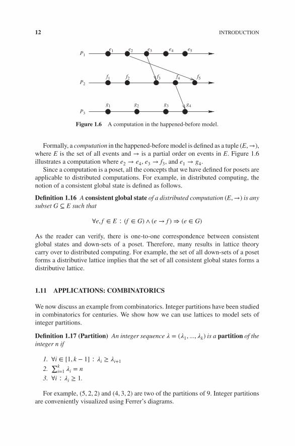
As mentioned earlier, posets have a wide range of applications. In this book, we willfocus on applications to distributed computing and combinatorics.
Partial order play an important role in distributed computing because a distributedcomputation is most profitably modeled as a partially ordered set of events. A dis-tributed program consists of two or more processes running on different processorsand communicating via messages. We will be concerned with a single computation ofsuch a distributed program. Each process Pi in that computation generates a sequenceof events. There are three types of events—internal, send, and receive. It is clear howto order events within a single process. If event e occurred before f in the process,then e is ordered before f . How do we order events across processes? If e is the sendevent of a message and f is the receive event of the same message, then we can order ebefore f . Combining these two ideas, we obtain the following definition.
Definition 1.15 (Happened-Before Relation) The happened-before relation (→)on a set of events E is the smallest relation on E that satisfies
1. If event e occurred before event f in the same process, then e → f ,
2. If e is the send event of a message and f is the receive event of the same message,then e → f , and
3. If there exists an event g such that (e → g) and (g → f ), then (e → f ).
12 INTRODUCTION
P1
P2
P3
e1 e2 e3 e4 e5
f1 f2 f3 f4 f5
g1 g2 g3 g4
Figure 1.6 A computation in the happened-before model.
Formally, a computation in the happened-before model is defined as a tuple (E,→),where E is the set of all events and → is a partial order on events in E. Figure 1.6illustrates a computation where e2 → e4, e3 → f3, and e1 → g4.
Since a computation is a poset, all the concepts that we have defined for posets areapplicable to distributed computations. For example, in distributed computing, thenotion of a consistent global state is defined as follows.
Definition 1.16 A consistent global state of a distributed computation (E,→) is anysubset G ⊆ E such that
∀e, f ∈ E ∶ (f ∈ G) ∧ (e → f ) ⇒ (e ∈ G)
As the reader can verify, there is one-to-one correspondence between consistentglobal states and down-sets of a poset. Therefore, many results in lattice theorycarry over to distributed computing. For example, the set of all down-sets of a posetforms a distributive lattice implies that the set of all consistent global states forms adistributive lattice.
1.11 APPLICATIONS: COMBINATORICS
We now discuss an example from combinatorics. Integer partitions have been studiedin combinatorics for centuries. We show how we can use lattices to model sets ofinteger partitions.
Definition 1.17 (Partition) An integer sequence 𝜆 = (𝜆1, ..., 𝜆k) is a partition of theinteger n if
1. ∀i ∈ [1, k − 1] ∶ 𝜆i ≥ 𝜆i+1
2.∑k
i=1 𝜆i = n
3. ∀i ∶ 𝜆i ≥ 1.
For example, (5, 2, 2) and (4, 3, 2) are two of the partitions of 9. Integer partitionsare conveniently visualized using Ferrer’s diagrams.

NOTATION AND PROOF FORMAT 13
Figure 1.7 Ferrer’s diagram for (4, 3, 2) shown to contain (2, 2, 2).
Definition 1.18 (Ferrer’s Diagram) A Ferrer’s diagram for an integer partition𝜆 = (𝜆1, ..., 𝜆k) of integer n is a matrix of dots where the ith row contains 𝜆i dots.Thus, row i represents the ith part and the number of rows represents the number ofparts in the partition.
We define an order on the partitions as follows: Given two partitions𝜆 = (𝜆1, 𝜆2,… , 𝜆m), 𝛿 = (𝛿1, 𝛿2,… , 𝛿n), we say that 𝜆 ≥ 𝛿 iff m ≥ n and∀i ∶ 1 ≤ i ≤ n, 𝜆i ≥ 𝛿i. This can also be viewed in terms of containment in theFerrer’s diagram, i.e. 𝜆 ≥ 𝛿 if the Ferrer’s diagram for 𝛿 is contained in the Ferrer’sdiagram of 𝜆. For example, consider the partitions (4, 3, 2) and (2, 2, 2). The Ferrer’sdiagram for (2, 2, 2) is contained in the Ferrer’s diagram for (4, 3, 2) as shown inFigure 1.7. Hence, (4, 3, 2) ≥ (2, 2, 2).
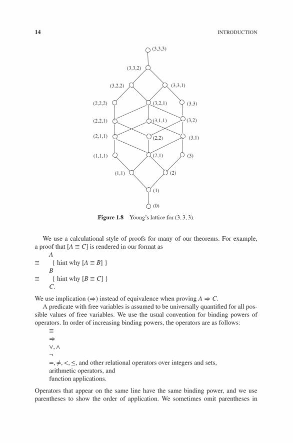
Definition 1.19 (Young’s Lattice) Given a partition 𝜆, Young’s lattice Y𝜆 is theposet of all partitions that are less than or equal to 𝜆.
The Young’s lattice for (3, 3, 3) is shown in Figure 1.8. Note that partitions less thana given partition are not necessarily partitions of the same integer.
Again, it follows easily from lattice theory that the Young’s lattice is distributive.Furthermore, assume that we are interested in only those partitions in Y𝜆 which havedistinct parts. The notion of slicing posets (explained in Chapter 10 can be used toanalyze such subsets of integer partitions.
1.12 NOTATION AND PROOF FORMAT
We use the following notation for quantified expressions:
(op free-var-list : range-of-free-vars : expression)
where op is a universal or an existential quantifier, free-var-list is the list of variablesover which the quantification is made, and the range-of-free-vars is the range of thevariables. For example, (∀i ∶ 0 ≤ i ≤ 10 ∶ i2 ≤ 100) means that for all i such that0 ≤ i ≤ 10, i2 ≤ 100 holds. If the range of the variables is clear from the context,then we simply use
(op free-var-list : expression).
For example, if it is clear that i and j are integers, then we may write
∀i ∶ (∃j ∶ j > i).
14 INTRODUCTION
(3,1,1)
(3)
(3,3,1)
(3,3,3)
(3,3)
(1)
(2,1)
(3,2,1)
(3,3,2)
(3,2,2)
(2,2,2)
(1,1,1)
(1,1) (2)
(0)
(3,1)(2,1,1)
(2,2,1) (3,2)
(2,2)
Figure 1.8 Young’s lattice for (3, 3, 3).
We use a calculational style of proofs for many of our theorems. For example,a proof that [A ≡ C] is rendered in our format as
A≡ { hint why [A ≡ B] }
B≡ { hint why [B ≡ C] }
C.
We use implication (⇒) instead of equivalence when proving A ⇒ C.A predicate with free variables is assumed to be universally quantified for all pos-
sible values of free variables. We use the usual convention for binding powers ofoperators. In order of increasing binding powers, the operators are as follows:
≡
⇒∨,∧¬=,≠, <,≤, and other relational operators over integers and sets,arithmetic operators, andfunction applications.
Operators that appear on the same line have the same binding power, and we useparentheses to show the order of application. We sometimes omit parentheses in

BIBLIOGRAPHIC REMARKS 15
expressions when they use operators from different lines. Thus
x ≤ y ∧ y ≤ z ⇒ x ≤ z
is equivalent to∀x, y, z ∶ (((x ≤ y) ∧ (y ≤ z)) ⇒ (x ≤ z)).
1.13 PROBLEMS
1.1. Give an example of a nonempty binary relation that is symmetric and transitivebut not reflexive.
1.2. The transitive closure of a relation R on a finite set can also be defined as thesmallest transitive relation on S that contains R. Show that the transitive closureis uniquely defined. We use “smaller” in the sense that R1 is smaller than R2 if|R1| < |R2|.
1.3. Show that if P and Q are posets defined on set X, then so is P ∩ Q.
1.4. Draw the Hasse diagram of all natural numbers less than 10 ordered by the rela-tion divides.
1.5. Show that if C1 and C2 are down-sets for any poset (E, <), then so is C1 ∩ C2.
1.6. Show the following properties of ⊔ and ⊓.
(L1) a ⊔ (b ⊔ c) = (a ⊔ b) ⊔ c (associativity)
(L1)𝛿 a ⊓ (b ⊓ c) = (a ⊓ b) ⊓ c
(L2) a ⊔ b = b ⊔ a (commutativity)
(L2)𝛿 a ⊓ b = b ⊓ a
(L3) a ⊔ (a ⊓ b) = a (absorption)
(L3)𝛿 a ⊓ (a ⊔ b) = a
1.7. Prove Lemma 1.7.
1.8. Prove Theorem 1.11.
1.9. Complete the proof of Theorem 1.12.
1.14 BIBLIOGRAPHIC REMARKS
The first book on lattice theory was written by Garrett Birkhoff [Bir40, Bir48, Bir67].The reader will find a discussion of the origins of lattice theory and an extensivebibliography in the book by Gratzer [Grä71, Grä03]. The book by Davey and Priestley

16 INTRODUCTION
[DP90] provides an easily accessible account of the field. Some other recent bookson lattice theory or ordered sets include books by Caspard, Leclerc, and Monjardet[CLM12], and Roman [Rom08]. The happened-before relation on the set of eventsin a distributed computation is due to Lamport [Lam78]. Reading [Rea02] gives adetailed discussion of dissectors and their properties. The proof format adopted formany theorems in this book is taken from Dijkstra and Scholten [DS90].

2REPRESENTING POSETS
2.1 INTRODUCTION
We now look at some possible representations for efficient queries and operations onposets. For this purpose, we first examine some of the common operations that aregenerally performed on posets. Given a poset P, the following operations on elementsx, y ∈ P are frequently performed:
1. Check if x ≤ y. We denote this operation by leq(x, y).2. Check if x covers y.
3. Compute x ⊓ y (meet(x, y)) and x ⊔ y (join(x, y)).
In all such representations, we first need to number the elements of the poset. A usefulway of doing this is discussed in Section 2.2. In the following sections, we considersome representations for posets and compare their complexity for the set of operationsmentioned earlier.
2.2 LABELING ELEMENTS OF THE POSET
Assume that a finite poset with n elements is given to us as a directed graph (Hassediagram), where nodes represent the elements in the poset and the edges representthe cover relation on the elements. We number the nodes, i.e., provide a label to eachnode from {1..n} such that if x < y then label(x) < label(y). This way we can answer
Introduction to Lattice Theory with Computer Science Applications, First Edition. Vijay K. Garg.© 2015 John Wiley & Sons, Inc. Published 2015 by John Wiley & Sons, Inc.

18 REPRESENTING POSETS
some queries of the form “Is x < y ?” directly without actually looking at the lists ofedges of the elements x and y. For example, if label(x) equals 5 and label(y) equals 3then we know that x is not less than y. Note that label(x) < label(y) does not necessar-ily imply that x < y. It only means that x ≯ y. One straightforward way of generatingsuch a labeling would be :
1. Choose a node x with in-degree 0 and assign the lowest available label to x.
2. Delete x and all outgoing edges from x.
3. Repeat steps 1 and 2 until there are no nodes left in the graph.
The above-mentioned procedure is called topological sort and it is easy to showthat it produces a linear extension of the poset. The procedure also shows that everyfinite poset has a linear extension. The following result due to Szpilrajn shows thatthis is true for all posets, even the infinite ones.
Theorem 2.1 ([Szp37]) Every partial order P has a linear extension.
Proof: Let be the set of all posets that extend P. Define a poset Q to be less than orequal to R if the relation corresponding to Q is included in the relation R. Consider amaximal element Z of the set 1. If Z is totally ordered, then we are done as Z is thelinear extension. Otherwise, assume that x and y are incomparable in Z. By addingthe tuple (x, y) to Z and computing its transitive closure, we get another poset in
that is bigger than Z contradicting maximality of Z.
2.3 ADJACENCY LIST REPRESENTATION
Since a poset is a graph, we can use an adjacency list representation for a graph. Inan adjacency list representation, we have a linked list for each element of the poset.We can maintain two relationships through an adjacency list :
1. Cover relation (e<c) : The linked list for element x ∈ P = {y|y ∈ P, x <c y}
2. Poset relation (e≤) : The linked list for element x ∈ P = {y|y ∈ P, x ≤ y}.
Figure 2.1 shows an example of a poset with its adjacency list representation forboth the relations. Choosing between the two relations for creating an adjacency listinvolves a trade-off. Representing e<c
requires less space, while most operations arefaster with the e≤ representation. For example, representing a chain of n elementsusing e<c
requires O(n) space as compared to O(n2) space using e≤. On the otherhand, checking x ≤ y for some elements x, y ∈ P requires time proportional to thesize of the linked list of x using e≤ as compared to O(n + |e<c
|) time using e<c.
For very large graphs, one can also keep all adjacent elements of a node in a(balanced) tree instead of a linked list. This can cut down the worst case complexity
1This step requires Zorn’s lemma, which is equivalent to the axiom of choice

ADJACENCY LIST REPRESENTATION 19
b
e
d
c
b
a a
c
b
e
d
Adjacency list for poset relation
b
e
c c
a
c
e
Poset
e
e
d
b
d
d
Adjacency list for cover relation
d
Figure 2.1 Adjacency list representation of a poset.
for answering queries of the form x <c y or x ≤ y. Balanced trees are standard datastructures and will not be discussed any further. For simplicity, we continue to uselinked lists and discuss algorithms when the poset is represented using adjacency listsfor (1) the cover relation or (2) the poset relation.
Since the adjacency list corresponds to the cover relation, the query “Does y coverx?” can be answered by simply traversing the linked list for node x. The query “Isx ≤ y?” requires a breadth-first search (BFS) or depth-first search (DFS) starting fromnode x resulting in time O(n + |e<c
|) as mentioned earlier.We now give an O(n + |e<c
|) algorithm to compute the join of two elementsx and y. The algorithm returns null if the join does not exist. To compute the join ofx and y, we proceed as follows:
• Step 0: Color all nodes white.
• Step 1: Color all nodes reachable from x as gray. This can be done by a BFS ora DFS starting from node x.
• Step 2: Do a BFS/DFS from node y. Color all gray nodes reached as black.
• Step 3: We now determine for each black node z, the number of black nodesthat point to z. Call this number inBlack[z] for any node z. This step can be per-formed in O(n + |e<c
|) by going through the adjacency lists of all black nodesand maintaining cumulative counts for inBlack array.
• Step 4: We count the number of black nodes z with inBlack[z] equal to 0. Ifthere is exactly one node, we return that node as the answer. Otherwise, wereturn null.
It is easy to see that a node is black iff it can be reached from both x and y. Wenow show that z equals join(x, y) iff it is the only black node with no black nodespointing to it. Consider the subgraph of nodes that are colored black. If this graphis empty, then there is no node that is reachable from both x and y and thereforejoin(x, y) is null as returned by our method. Otherwise, the subgraph of black nodesis nonempty. Owing to acyclicity and finiteness of the graph, there is at least one nodewith inBlack equal to 0. If there are two or more nodes with inBlack equal to 0, thenthese are incomparable upper bounds and therefore join(x, y) does not exist. Finally,if z is the only black node with inBlack equal to 0, then all other black nodes arereachable from z because all black nodes are reachable from some black node withinBlack equal to 0. Therefore, z is the least upper bound of x and y.

20 REPRESENTING POSETS
Now assume that the adjacency list of x includes all elements that are greater thanor equal to x, i.e., it encodes the poset relation (e≤). Generally, the following opti-mization is made for representation of adjacency lists. We keep the adjacency list ina sorted order. This enables us to search for an element in the list faster. For example,if we are looking for node 4 in the list of node 1 sorted in ascending order and weencounter the node 6, then we know that node 4 cannot be present in the list. Wecan then stop our search at that point instead of looking through the whole list. Thisoptimization results in a better average case complexity.
Let us now explore complexity of various queries in this representation. To checkthat y covers x, we need to check that x ≤ y and for any z different from x and y suchthat x ≤ z, z ≤ y is not true. This can be easily done by going through the adjacencylists of all nodes that are in the adjacency list of x and have labels less than y inO(n + |e≤|) time.
Checking x ≤ y is trivial, so we now focus on computing join(x, y).
• Step 0: We take the intersection of the adjacency lists of nodes x and y. Sincelists are sorted, this step can be done in O(ux + uy) time where ux and uy are thesize of the adjacency lists of x and y, respectively. Call this list U.
• Step 1: If U is empty, we return null. Otherwise, let 𝑤 be the first element in thelist.
• Step 2: if U is contained in the adjacency list of 𝑤, we return 𝑤; else, we returnnull.
A further optimization that can lead to reduction in space and time complexityfor dense posets is based on keeping intervals of nodes rather than single nodes inadjacency lists. For example, if the adjacency list of node 2 is {4, 5, 6, 8, 10, 11, 12},then we keep the adjacency list as three intervals {4 − 6, 8 − 8, 10 − 12}. We leavethe algorithms for computing joins and meets in this representation as an exercise.
2.4 VECTOR CLOCK REPRESENTATION
Of all operations performed on posets, the most fundamental is leq(x, y). We haveobserved that by storing just the cover relation, we save on space but have to spendmore time to check leq(x, y). On the other hand, keeping the entire poset relation canbe quite wasteful as the adjacency lists can become large as the number of nodes inthe poset increase. We now show a representation that provides a balance betweenthe cover relation and the poset relation. This representation, called vector clock rep-resentation, assumes that the poset is partitioned into k chains for some k. Algorithmsfor partitioning posets into the minimum number of chains is discussed in Chapter 3.For vector clock representation, we do not require the partition to have the least num-ber of chains.
Let there be k chains in some partition of the poset. All elements in any chain aretotally ordered and we can rank them from 1 to the total number of elements in the
VECTOR CLOCK REPRESENTATION 21
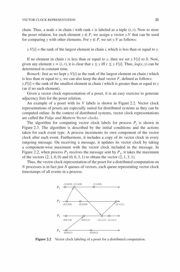
chain. Thus, a node x in chain i with rank r is labeled as a tuple (i, r). Now to storethe poset relation, for each element y ∈ P, we assign a vector y.V that can be usedfor comparing y with other elements. For y ∈ P, we set y.V as follows:
y.V[i] = the rank of the largest element in chain i, which is less than or equal to y.
If no element in chain i is less than or equal to y, then we set y.V[i] to 0. Now,given any element x = (i, r), it is clear that x ≤ y iff r ≤ y.V[i]. Thus, leq(x, y) can bedetermined in constant time.
Remark: Just as we kept y.V[i] as the rank of the largest element on chain i whichis less than or equal to y, we can also keep the dual vector F, defined as follows:y.F[i] = the rank of the smallest element in chain i which is greater than or equal to y(∞ if no such element).
Given a vector clock representation of a poset, it is an easy exercise to generateadjacency lists for the poset relation.
An example of a poset with its V labels is shown in Figure 2.2. Vector clockrepresentations of posets are especially suited for distributed systems as they can becomputed online. In the context of distributed systems, vector clock representationsare called the Fidge and Mattern Vector clocks.
The algorithm for computing vector clock labels for process Pj is shown inFigure 2.3. The algorithm is described by the initial conditions and the actionstaken for each event type. A process increments its own component of the vectorclock after each event. Furthermore, it includes a copy of its vector clock in everyoutgoing message. On receiving a message, it updates its vector clock by takinga component-wise maximum with the vector clock included in the message. InFigure 2.2, when process P3 receives the message sent by P1, it takes the maximumof the vectors (2, 1, 0, 0) and (0, 0, 3, 1) to obtain the vector (2, 1, 3, 1).
Thus, the vector clock representation of the poset for a distributed computation onN processes is in fact just N queues of vectors, each queue representing vector clocktimestamps of all events in a process.
(0,0,0,1) (0,0,0,2)
(3,1,0,0)
(2,1,3,1)
(2,1,0,0)
(0,0,2,1) (2,1,4,1)
(0,2,0,0) (2,3,3,1)
(0,0,1,0)
(0,1,0,0)
(1,0,0,0)P1
P2
P3
P4
Figure 2.2 Vector clock labeling of a poset for a distributed computation.

22 REPRESENTING POSETS
Pj::var
V: array[1…N] of integerinitially (∀i ∶ i ≠ j ∶ V[i] = 0) ∧ (V[j] = 1);
send event :V[j] ∶= V[j] + 1;
receive event with vector WV[j] ∶= V[j] + 1;for i ∶= 1 to N do
V[i] ∶= max(V[i],W[i]);
internal eventV[j] ∶= V[j] + 1
Figure 2.3 Vector clock algorithm.
2.5 MATRIX REPRESENTATION
Like a directed graph, a poset can also be represented using a matrix. If there is a posetP with n nodes, then it can be represented by a matrix A of size n × n. As before, wecan either represent the cover relation or the poset relation through the matrix. Sincein both cases we would be using O(n2) space, we generally use a matrix representationfor the poset relation. Thus, for xi, xj ∈ P, xi ≤ xj iff A[i, j] = 1. The main advantageof using the matrix representation is that it can answer the query “Is x ≤ y?” in O(1)time.
2.6 DIMENSION-BASED REPRESENTATION
The motivation for the dimension-based representation comes from the fact that in thevector clock algorithm, we require O(k) components in the vector where k is boundedby the smallest number of chains required to decompose the poset. As we will see inChapter 3, Dilworth’s Theorem shows that the least number of chains required equalsthe width of the poset. So, the natural question to ask is if there exists an alternate wayof timestamping elements of a poset with vectors that requires less components thanthe width of the poset and can still be used to answer the query of the form leq(x, y).
Surprisingly, in some cases, we can do with fewer components. For example,consider the poset shown in Figure 2.4(a). Since the poset is just an antichain, the min-imum number of chains required to cover the poset is 5. So for using the vector clockrepresentation, we require five components in the vector. But consider the followingtwo linear extensions of the poset : x1, x2, x3, x4, x5 and x5, x4, x3, x2, x1, shown in

ALGORITHMS TO COMPUTE IRREDUCIBLES 23
x1
(a)
(b)
x2 x3 x4 x5
x1
x2
x3
x4
x5 x1
x2
x3
x4
x5
Figure 2.4 (a) An antichain of size 5 and (b) its two linear extensions.
Figure 2.4(b). Using the ranks of the elements in these two linear extensions, weget the following vectors : (1, 5), (2, 4), (3, 3), (4, 2), and (5, 1). These vectors haveone-to-one correspondence with the poset order, i.e., they form an antichain. So inthis case, we can get away with just 2 components in the vector. This idea of using lin-ear extensions of the poset to assign a vector to each element can be generalized to anyposet. The minimum number of linear extensions required is called the dimension ofthe poset. More formally, we first define a realizer of a poset.
Definition 2.2 (Realizer) A family R = {L1,L2,… ,Lt} of linear extensions of aposet P on X is called a realizer of P if
P = ∩Li∈RLi.
The dimension of a poset P is the size of the smallest realizer. Determining thedimension of a given poset is NP-hard, whereas determining the width of a poset iscomputationally easy. For this reason, the dimension based representation is generallynot used in distributed systems even though the dimension may be smaller than thewidth of the poset. The concept of dimension and related results are described in moredetail in Chapter 16
2.7 ALGORITHMS TO COMPUTE IRREDUCIBLES
In this section, we briefly consider algorithms for determining irreducibles of aposet. Assume that we have the adjacency list representation of the cover relation. Todetermine whether x is join-irreducible we first compute LC(x), the set of elementscovered by x. Then, we use the following procedure to check if x is join-irreducible.
24 REPRESENTING POSETS
• Step 1: If LC(x) is singleton, return true;
• Step 2: If LC(x) is empty, thenif x is the minimum element of the poset, return false, else return true;
• Step 3: If join(LC(x)) exists then return false, else return true.
The complexity of this procedure is dominated by the third step that takes O(n +e<c
) in the worst case. The proof of correctness of the procedure is left as an exercise.
2.8 INFINITE POSETS
We now consider the representation of (countably) infinite posets for computingapplications. Since computers have finite memory, it is clear that we will have to usefinite representation for these posets. We assume that the infinite poset is “periodic”(a concept that will be explained later) to enable us finite representation of infiniteposets. Our representation is motivated by the need for modeling infinite distributedcomputations.
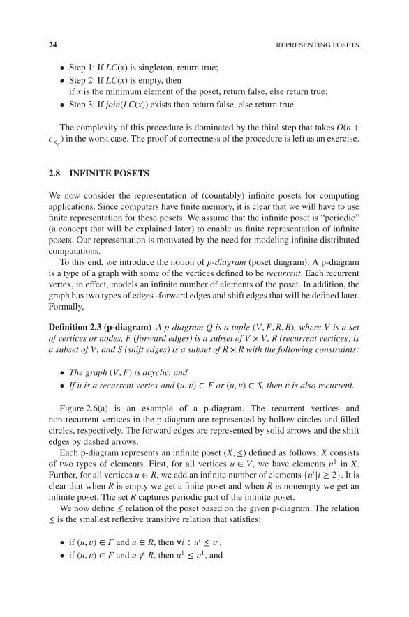
To this end, we introduce the notion of p-diagram (poset diagram). A p-diagramis a type of a graph with some of the vertices defined to be recurrent. Each recurrentvertex, in effect, models an infinite number of elements of the poset. In addition, thegraph has two types of edges -forward edges and shift edges that will be defined later.Formally,
Definition 2.3 (p-diagram) A p-diagram Q is a tuple (V ,F,R,B), where V is a setof vertices or nodes, F (forward edges) is a subset of V × V, R (recurrent vertices) isa subset of V, and S (shift edges) is a subset of R × R with the following constraints:
• The graph (V ,F) is acyclic, and
• If u is a recurrent vertex and (u, 𝑣) ∈ F or (u, 𝑣) ∈ S, then 𝑣 is also recurrent.
Figure 2.6(a) is an example of a p-diagram. The recurrent vertices andnon-recurrent vertices in the p-diagram are represented by hollow circles and filledcircles, respectively. The forward edges are represented by solid arrows and the shiftedges by dashed arrows.
Each p-diagram represents an infinite poset (X,≤) defined as follows. X consistsof two types of elements. First, for all vertices u ∈ V , we have elements u1 in X.Further, for all vertices u ∈ R, we add an infinite number of elements {ui|i ≥ 2}. It isclear that when R is empty we get a finite poset and when R is nonempty we get aninfinite poset. The set R captures periodic part of the infinite poset.
We now define ≤ relation of the poset based on the given p-diagram. The relation≤ is the smallest reflexive transitive relation that satisfies:
• if (u, 𝑣) ∈ F and u ∈ R, then ∀i ∶ ui ≤ 𝑣i,
• if (u, 𝑣) ∈ F and u ∉ R, then u1 ≤ 𝑣1, and

INFINITE POSETS 25
• if (u, 𝑣) ∈ S, then ui ≤ 𝑣i+1.
We now have the following theorem.
Theorem 2.4 (X,≤) as defined above is a reflexive poset.
Proof: We show that ≤ is reflexive, transitive, and antisymmetric. It is reflexive andtransitive by construction. We now show that ≤ as defined earlier does not createany nontrivial cycle (cycle of size greater than one). Any cycle in elements of theposet with the same index would imply cycle in (V ,F). Thus, any cycle would haveelements with at least two indices. However, the relation ≤ never makes a higherindexed element smaller than a lower indexed element.
Let us now consider some examples.
1. The set of natural numbers with the usual order can be modeled using thep-diagram shown in Figure 2.5(a), whereV = {u}; F = {}; S = {(u, u)}; R = {u}.Note that this poset has infinite height and width equal to 1.
2. The set of natural numbers with no order can be modeled as shown inFigure 2.5(b) withV = {u}; F = {}; S = {}; R = {u}.
3. Figure 2.6 shows an example of a p-diagram along with the correspondinginfinite poset. This p-diagram captures infinite behavior of a distributedcomputation.
We cannot expect finite p-diagrams to be able to model all infinite posets. We nowgive some examples of posets that cannot be represented using p-diagrams.
(a) (b)
Figure 2.5 (a,b) Trivial examples of p-diagrams.
g
f
ea
b
c
d
(a) (b)
a1 d1 e1 d2 e2 d3 e3
b1 f1
c1 g1
f 2
g2
f 3
g3
Figure 2.6 (a) A p-diagram and (b) its corresponding infinite poset.

26 REPRESENTING POSETS
1. The set of all integers (including negative integers) under the usual order rela-tion cannot be represented using a p-diagram. The set of integers does not haveany minimal element. Any poset defined using a p-diagram is well-founded.
2. Consider the set of all natural numbers with the order that all even numbersare less than all the odd numbers. This poset cannot be represented using ap-diagram. In this poset, the set of elements that cover some element may beinfinite. For example, the number 2 is covered by an infinite number of ele-ments. In a p-diagram, an element can only have a bounded number of lowerand upper covers.
The following properties of a p-diagram posets are easy to show.
Lemma 2.5 A poset P defined by a p-diagram has the following properties:
1. P is well-founded.
2. There exists a constant k such that the size of the set of upper covers and lowercovers of every element is bounded by k.
Runs of a distributed computation generated by a finite number of processes havefinite width. The following lemma characterizes those p-diagrams for which the cor-responding posets have finite width.
Lemma 2.6 A poset P defined by a p-diagram has finite width iff for every recurrentvertex there exists a cycle in the graph (R,F ∪ S).
Proof: If every recurrent vertex 𝑣 is in a cycle, then we get that the set
{𝑣i|i ≥ 1}
is totally ordered. This implies that the poset can be decomposed into a finite numberof chains and therefore has a finite width. Conversely, if there exists any recurrentvertex 𝑣 that is not in a cycle, then 𝑣i is incomparable to 𝑣j for all i, j. Then, the set
{𝑣i|i ≥ 1}
forms an antichain of infinite size. Thus, P has infinite width.
Algorithms to check whether x ≤ y or x covered by y are left as an exercise.
2.9 PROBLEMS
2.1. Design algorithms for performing the common poset operations for the matrixrepresentation and analyze their time complexity.

BIBLIOGRAPHIC REMARKS 27
2.2. Give efficient algorithms for calculating the join and meet of the elements of aposet using the dimension representation.
2.3. Give parallel and distributed algorithms for topological sort.
2.4. Give parallel and distributed algorithms for computing the poset relation fromthe cover relation.
2.5. Give parallel and distributed algorithms for computing x ⊔ y in various repre-sentations.
2.6. Give an efficient algorithm to convert a vector clock representation of posetinto an adjacency list representation of the poset relation.
2.7. (Open) How many different (non-isomorphic) posets can be defined on n ele-ments?
2.8. (Open) Given two posets P and Q, what is the complexity of checking whetherthey are isomorphic?
2.9. Give an efficient algorithm that takes a poset as input and returns all its irre-ducibles and dissectors.
2.10. Give efficient algorithms to determine x ⊔ y, leq(x, y) and isco𝑣eredby(x, y) forelements x and y in a p-diagram.
2.11. Give an algorithm to compute the width of a p-diagram.
2.10 BIBLIOGRAPHIC REMARKS
The reader is referred to the book by Cormen, Leiserson, Rivest, and Stein [CLRS01]for details on topological sort and adjacency representation of graphs. Vector clockrepresentation in distributed systems is due to Fidge [Fid89] and Mattern [Mat89].The dimension-based representation of posets is due to Dushnik and Miller [DM41].The discussion of p-diagrams is taken from the paper by Agarwal, Garg, and Ogale[AGO10].

3DILWORTH’S THEOREM
3.1 INTRODUCTION
Of all the results in lattice theory, perhaps the most famous is Dilworth’s Theorem fordecomposition of a poset. Dilworth’s Theorem belongs to the special class of results,called min–max results, which relate a maximal value in a structure to a minimalvalue. Dilworth’s Theorem states that the minimum number of chains a poset can bepartitioned into equals the maximum size of an antichain. In this chapter, we coverthis result and associated algorithms.
3.2 DILWORTH’S THEOREM
We first present a proof of Dilworth’s Theorem due to Galvin [Gal94].
Theorem 3.1 ([Dil50]) [Dilworth’s Theorem] Any finite poset P = (X,≤) of width𝑤 can be decomposed into 𝑤 chains. Furthermore, 𝑤 chains are necessary for anysuch decomposition.
Proof: We begin by proving that 𝑤 chains are necessary and that it is not possibleto decompose the poset into less than 𝑤 chains. Consider the longest antichain (oflength 𝑤). Each element of this antichain must belong to a separate chain in the chaindecomposition of the poset and hence we need at least 𝑤 chains.
Introduction to Lattice Theory with Computer Science Applications, First Edition. Vijay K. Garg.© 2015 John Wiley & Sons, Inc. Published 2015 by John Wiley & Sons, Inc.

30 DILWORTH’S THEOREM
x
C
C1 C2 Ci Ct
a1 a2 ai at
Figure 3.1 Decomposition of P into t chains.
We now show that 𝑤 chains are indeed sufficient to completely partition the poset.The proof is by induction on n, the size of the poset. The base case n = 1 is simplebecause a poset containing one element can be partitioned into one chain containingthat element.
Consider a poset P of size n. Let x denote a maximal element of P. Consider thesubposet P′ = (X − {x},≤). Since this is a poset of size less than n, by the inductionhypothesis, we can decompose it into t disjoint chains where t is the width of P′. LetC1, ...,Ct denote the chains obtained after decomposition. We are required to provethat either P has an antichain of size t + 1 or P is a union of t chains.
Let ai be the maximal element of Ci, which is part of some antichain of size t. Theset A = {a1, ..., at} forms an antichain. To see this, consider an antichain containingaj. There exists bi ∈ Ci, which belongs to this antichain because any antichain ofsize t must have exactly one element from each chain Ci. Since ai is the maximumelement in the chain Ci which is part of some antichain of size t, bi ≤ ai. Therefore,bi||aj implies that ai ≰ aj.
We now compare x with all the elements of A. If A ∪ {x} forms an antichain, thenthe width of P is t + 1 and the chain decomposition of P is C1, ...,Ct, {x}. Otherwise,there exists ai ∈ Ci such that ai < x for some i. The set C = {y ∈ Ci | y ≤ ai} forms achain in P. Since ai is the maximal element in Ci that is a part of some t-sized antichainin P, the width of Q = (X − C,≤) is less than t. Then, by the induction hypothesis,we can partition Q into t − 1 chains. Hence along with C, this forms a decompositionof P into t chains (Figure 3.1).
Any partition of a poset into chains is also called a chain cover of the poset.
3.3 APPRECIATION OF DILWORTH’S THEOREM
This was one of our first nontrivial proofs in the book. A delightful result such asDilworth’s Theorem must be savored and appreciated. We now look at a few questionsthat naturally arise out of the above proof which will help the reader understand theproof better.

APPRECIATION OF DILWORTH’S THEOREM 31
For any nontrivial proof, the reader should try out special cases. For example, inDilworth’s Theorem, one may consider the special case of posets of height 1 (i.e.,a bipartite graph). In this case, one obtains the Konig–Egervary Theorem discussedin Section 3.8.
In any substantial proof, it is generally useful to find lemmas that can be abstractedout of this proof and reused in other proofs. In the proof of Dilworth’s Theorem, thekey ingredient was to prove that the set A is an antichain. This gives us the followingresult.
Theorem 3.2 Let A𝑤 be the set of all antichains of size 𝑤 in a finite poset P of width𝑤. Let {C1,C2, ...,C𝑤} be a decomposition of P into 𝑤 chains. For Y, any antichainof size 𝑤, let Y[i] denote the element in Y from chain Ci. We define an order ⪯ on A𝑤
as follows:
Y ⪯ Zdef= ∀i ∶ Y[i] ≤ Z[i] for all Y ,Z ∈ A𝑤,
Then, (A𝑤,⪯) is a lattice.
Proof: Given Y ,Z ∈ A𝑤, we define a set formed by
W[i] ∶= min(Y[i], Z[i]).
We first show that W ∈ A𝑤. It is sufficient to show that W[i]||W[j] for any i and j.By symmetry, it is sufficient to show that W[i] ≮ W[j]. Without loss of generality, letW[i] = Y[i]. If W[j] = Y[j], then W[i] ≮ W[j] follows from Y ∈ A𝑤. If W[j] = Z[j],then W[i] ≮ W[j] follows from Z[j] ≤ Y[j] and Y[i] ≮ Y[j]. It is easy to see that W isthe meet of Y and Z.
A dual argument holds for the join of Y and Z.
To appreciate a nontrivial theorem, one must look for alternative proofs. Forexample, we used induction on the size of the poset in our proof. Here we giveanother proof which is based on removing a chain instead of an element as inGalvin’s proof. This is closer to Dilworth’s original proof [Dil50].
Sketch of an Alternative Proof: Let P be a poset of width k. For induction, weassume that any poset with smaller cardinality of width 𝑤 or less can be partitionedinto 𝑤 chains. If P is an empty relation (i.e., has no comparable elements), then Phas exactly k elements and can be trivially decomposed into k chains. Otherwise,consider a chain C = {x, y} where x is a minimal element and y a maximal elementof P. If the width of P − C is less than k, we are done because we can use that partitioncombined with C to get the desired partition. If the width of P − C is k, then thereexists an antichain A of size k in the subposet P − C. We consider the subposets U[A]and D[A]. Since x ∉ U[A] and y ∉ D[A], we know that both U[A] and D[A] are strictlysmaller than P. By induction, each of these sets can be partitioned into k chains andsince U[A] ∩ D[A] = A, we can combine these chains to form the partition of theoriginal set.
◾
32 DILWORTH’S THEOREM
3.4 DUAL OF DILWORTH’S THEOREM
In lattice theory, one must also explore the duals of any nontrivial theorem. ForDilworth’s Theorem, we get the following result.
Theorem 3.3 ([Mir71]) Any poset P = (X,≤) of height h can be decomposed into hantichains. Furthermore, h antichains are necessary for any such decomposition.
Proof: All minimal elements of a poset form an antichain. When we delete thisantichain, the height of the poset decreases by exactly one. By continuing this proce-dure, we get the desired decomposition. The necessity part follows from the fact thatno two elements of a chain can be in the same antichain.
3.5 GENERALIZATIONS OF DILWORTH’S THEOREM
We can generalize Dilworth’s Theorem in the following manner:
1. Go from finite posets to infinite ones.
2. Generalize the theorem to directed graphs.
3. Decompose the poset into other structures, like k-families. A k-family in aposet P is a subposet containing no chains of size k + 1. So, an antichain formsa 1−family. We can try to generalize the dual of Dilworth’s Theorem to thisstructure.
Different proofs and their generalizations can be found in the literature. We referthe interested reader to West [Wes04].
3.6 ALGORITHMIC PERSPECTIVE OF DILWORTH’S THEOREM
In practical applications, it may not be sufficient to prove existence of a chain parti-tion. One may be required to compute it. Thus, from an algorithmic perspective, onecan look at the following questions:
1. How can we convert the proof of the theorem into an algorithm for chaindecomposition of a poset?
2. Given any algorithm for chain decomposition, we analyze its time and spacecomplexity. The natural question to ask is if we can improve the algorithmcomplexity or prove lower bounds on the time and space complexity.
3. Given any sequential algorithm, one can study variations of the algorithm thatcater to different needs. A parallel algorithm tries to speed up the computa-tion by using multiple processors. A distributed algorithm assumes that theinformation about the poset is distributed across multiple machines. An onlinealgorithm assumes that the elements of the poset are presented one at a time,

APPLICATION: HALL’S MARRIAGE THEOREM 33
and we maintain a chain decomposition at all times. The new element is insertedinto one of the existing chains or into a new chain. The online algorithm can-not change the existing chain decomposition and as a result may require morechains than an offline algorithm. An incremental algorithm also assumes thatelements of the poset are presented one at a time. The algorithm must computethe chain decomposition as we are presented with the new element. However,the algorithm is free to rearrange existing elements into chains when a newelement arrives. The key issue here is to avoid recomputing the chain decom-position for the entire poset whenever a new element is presented.
We will explore such algorithmic questions in Section 4.2. For now, we look atsome applications of Dilworth’s Theorem.
3.7 APPLICATION: HALL’S MARRIAGE THEOREM
In this section, we show the relationship between the problem of chain partition of aposet and matching in a bipartite graph. This relationship allows us to use the bipartitematching algorithms for chain-partition and vice versa.
We first describe an application of Dilworth’s Theorem to combinatorics. We aregiven a set of m girls G = {y1, ..., ym} and n boys B = {x1, ..., xn} with m ≤ n. Eachgirl yi has a set of boys S(yi) whom she is willing to marry. The aim is to find acondition on these sets so that it is possible to find a pairing of the girls and boyswhich enables each girl to get married. Each boy chosen from the set S(yi) must bedistinct. This problem is also known as computing the set of distinct representatives.
A solution to this problem is given by the following theorem. Let I ⊆ G. DefineS(I) =
⋃yi∈I S(yi).
Theorem 3.4 [Hall’s Theorem] The necessary and sufficient condition for theabove-mentioned set of distinct representatives problem is ∀I ⊆ G, |S(I)| ≥ |I|.
Proof: The necessary part of the condition is trivial because if I is smaller than S(I)then there will not be enough boys for pairing off with the girls. To prove that theabove-mentioned condition is sufficient, we assume that the given condition holdsand view the S relation as a poset of height 1 (Figure 3.2). This forms a bipartite poset.If we can split it into n chains then we are done. Thus, we need to prove that there is noantichain in the poset of size greater than |B| = n. Let A be an antichain of the posetand I = A ∩ G (all the girls included in the antichain A). Since A is an antichain, it doesnot contain an element belonging to S(I). Hence, |A| ≤ |I| + |B| − |S(I)| ≤ |B| as|I| ≤ |S(I)| from Hall’s condition. Thus, the maximum size of an antichain is |B| = n.By Dilworth’s Theorem, the poset can be partitioned into n chains. Since the antichainB is maximal, each chain in such a partition must contain exactly one point of B. Thus,we can take the chains in the partition of the poset, which contain points of G. Thesegive the desired pairings of boys and girls such that all the girls can get married. Thisproves the sufficiency of the given condition.

34 DILWORTH’S THEOREM
x1Set of Boys B
Set of Girls G
xn
y1 ym
Figure 3.2 Hall’s Marriage Theorem.
3.8 APPLICATION: BIPARTITE MATCHING
We now show applications of Dilworth’s Theorem to bipartite matching. A matchingin a graph G = (V ,E) is a subset of edges E′ ⊆ E such that no two edges in E′ haveany vertex in common. A vertex cover in a graph is a subset of vertices V ′ ⊆ V suchthat for every edge (x, y) ∈ E, either x ∈ V ′ or y ∈ V ′.
Theorem 3.5 (Konig–Egervary Theorem[Kon31, Ege31]) In a bipartite graph,the maximum size of a matching equals the minimum size of a vertex cover.
Proof: Let G = (L,R,E) be the bipartite graph with a total of n = |L| + |R| vertices.View this bipartite graph as a poset with vertices in L as the minimal vertices and R asthe maximal vertices. Any chain decomposition of this poset can have chains of sizeeither 1 or 2. We observe that
1. Any chain cover of size m ≤ n is equivalent to existence of a matching of sizen − m.
2. Any antichain in the poset corresponds to an independent set in the graph. Thus,the complement of an antichain corresponds to a vertex cover of the graph.Hence, existence of any antichain of size m is equivalent to existence of a vertexcover of size n − m.
From Dilworth’s theorem, the size of the biggest antichain equals the size of thesmallest chain cover. Therefore, the size of the smallest vertex cover equals the sizeof the largest matching.
The above-mentioned construction shows that by using chain decomposition, onecan solve the problem of bipartite matching. Now, we consider the converse. Assumethat we have an algorithm for bipartite matching. How do we use it for chain decom-position? This relationship between chain decomposition and bipartite matching isbased on the idea of a strict split of a poset.

ONLINE DECOMPOSITION OF POSETS 35
Definition 3.6 (Strict Split of a Poset) Given a poset P, the strict split of the posetP, denoted by S(P) is a bipartite graph (L,R,E) where L = {x−|x ∈ P}, R = {x+|x ∈P}, and E = {(x−, y+)|x < y in P}.
We state the following theorem due to Fulkerson [Ful56] whose proof is left as anexercise.
Theorem 3.7 Any matching in S(P) can be reduced to a chain cover of P.
Thus, one can use any algorithm for bipartite matching to determine a chain cover.There are many techniques available for bipartite matching. One can use augment-ing path algorithms that start with the trivial matching and increase the size of thematching one edge at a time. In a graph of n vertices and m edges, these algorithmstake O(mn) time. Hopcroft and Karp have given an O(m
√n) algorithm for bipartite
matching [HK71].It is important to note that bipartite matching can also be solved by a more
general technique of computing max-flows which itself is a special case of linearprogramming.
3.9 ONLINE DECOMPOSITION OF POSETS
Dilworth’s Theorem states that a finite poset of width k requires at least k chainsfor decomposition [Dil50]. However, constructive proofs of this result require theentire poset to be available for the partition. The best known online algorithm forpartitioning the poset is due to Kierstead [Kie81] which partitions a poset of widthk into (5k − 1)∕4 chains. The lower bound on this problem, due to Szemérdi (1982),states that there is no online algorithm that partitions all posets of width k into fewerthan
(k+12
)chains.
We will focus on a special version of the problem where the elements are presentedin a total order consistent with the poset order. Felsner [Fel97] has shown that evenfor the simpler problem, the lower bound of
(k+12
)holds. As an insight into the general
result, we show how any algorithm can be forced to use 3 chains for a poset of width 2.Consider the poset given in Figure 3.3. Initially, two incomparable elements x and yare presented to the chain decomposition algorithm. It is forced to assign x and yto different chains. Now an element z greater than both x and y is presented. If thealgorithm assigns z to a new chain, then it has already used three chains for a posetof width 2. Otherwise, without loss of generality, assume that the algorithm assignsz to x’s chain. Then, the algorithm is presented an element u, which is greater than xand incomparable to y and z. The algorithm is forced to assign u to a new chain andhence the algorithm uses three chains for a poset of width 2.
Furthermore, Felsner showed the lower bound to be strict and presented an algo-rithm that requires at most
(k+12
)chains to partition a poset. We present a simple
algorithm, owing to Agarwal and Garg [AG05], which partitions a poset into at most(k+12
)chains and requires at most O(k2) work per element.

36 DILWORTH’S THEOREM
x u
y z
Figure 3.3 A poset of width 2 forcing an algorithm to use three chains for decomposition.
varB1,… ,Bk: sets of queues
∀i ∶ 1 ≤ i ≤ k, |Bi| = i∀i ∶ q ∈ Bi, q is empty
When presented with an element z:for i = 1 to k
if ∃q ∈ Bi ∶ q is empty or q.head < zinsert z at the head of q;if i > 1
swap the set of queues Bi−1 and Bi ⧵ {q};
Figure 3.4 Chain partitioning algorithm.
The algorithm for online partitioning of the poset into at most(k+1
2
)chains is
shown in Figure 3.4. The algorithm maintains(k+1
2
)chains as queues partitioned into
k sets B1,B2, ...,Bk such that Bi has i queues. Let z be the new element to be inserted.We find the smallest i such that z is comparable with heads of one of the queues in Bior one of the queues in Bi is empty. Let this queue in Bi be q. Then, z is inserted atthe head of q. If i is not 1, queues in Bi−1 and Bi ⧵ {q} are swapped. Every elementof the poset is processed in this manner, and in the end, the nonempty set of queuesgives us the decomposition of the poset.
The following theorem gives the proof of correctness of the algorithm.
Theorem 3.8 The algorithm in Figure 3.4 partitions a poset of width k into(k+1
2
)
chains.
Proof: We claim that the algorithm maintains the followings invariant:
(I) For all i: Heads of all nonempty queues in Bi are incomparable with eachother.
Initially, all queues are empty and so the invariant holds. Suppose that theinvariant holds for the first m elements. Let z be the next element presented to the

A LOWER BOUND ON ONLINE CHAIN PARTITION 37
algorithm. The algorithm first finds a suitable i such that z can be inserted into oneof the queues in Bi.
Suppose the algorithm was able to find such an i. If i = 1, then z is inserted into B1and the invariant is trivially true. Assume i ≥ 2. Then, z is inserted into a queue q inBi which is either empty or has a head comparable with z. The remaining queues inBi are swapped with queues in Bi−1. After swapping, Bi has i − 1 queues from Bi−1and the queue q, and Bi−1 has i − 1 queues from Bi ⧵ {q}. The heads of queues inBi−1 are incomparable as the invariant I was true for Bi before z was inserted. Theheads of queues in Bi which originally belonged to Bi−1 are incomparable to eachother because of the invariant I. The head of q, z, is also incomparable to the headsof these queues as i was the smallest value such that the head of one of the queues inBi was comparable to z. Hence, the insertion of the new element still maintains theinvariant.
If the algorithm is not able to insert z into any of the queues, then all queue headsand in particular, queue heads in Bk are incomparable to z. Then, z along with thequeue heads in Bk form an antichain of size k + 1. This leads to a contradiction as thewidth of the poset is k. Hence, the algorithm is always able to insert an element intoone of the queues and the poset is partitioned into fewer than
(k+12
)chains.
Note that our algorithm does not need the knowledge of k in advance. It starts withthe assumption of k = 1, i.e., with B1. When a new element cannot be inserted into B1,we have found an antichain of size 2 and B2 can be created. Thus, the online algorithmuses at most
(k+12
)chains in decomposing posets without knowing k in advance.
This algorithm can be easily extended for online chain decomposition when thenew elements are either maximal elements or minimal elements of the poset seen sofar (see Problem 7).
3.10 A LOWER BOUND ON ONLINE CHAIN PARTITION
We now show a lower bound on the number of chains required for online chain parti-tion in the worst case. We will cast our problem in terms of a game between Alice andBob where Alice corresponds to the algorithm that does the online chain partition andBob corresponds to the adversary that provides the partial order. The goal for Aliceis to use as few chains as possible and for Bob to force Alice to use as many chainsas possible. We will require Bob to present elements of the poset only in increasingorder. We now claim:
Theorem 3.9 There exists a strategy for Bob that can force Alice to use(k+1
2
)chains.
Proof: Let the chains of the poset produced by decomposition be Ci and top(i) bethe maximal element of the chain Ci. If x is the maximal element of the poset, thenpri𝑣ate(x) is the set of chains Ci such that top(i) ≤ x and top(i) ≰ y for all maximalelements y ≠ x.

38 DILWORTH’S THEOREM
Induction Hypothesis : For every positive integer k, there is a strategy S(k) for Bobso that the poset P presented so far is of width k and has exactly k maximal elementsx1,… , xk such that for all i, |pri𝑣ate(xi)| ≥ i.Base Case : For k = 1, we use one element from process 1. The hypothesis holds forthis case.Induction Step : Suppose we have strategy S(k). We construct S(k + 1) using S(k) asfollows:
1. Run strategy S(k). This phase ends with an order Q1 with maximal elementsx1,… , xk, |pri𝑣ate(xi)| ≥ i.
2. Run strategy S(k) again. This time every new element is made greater than eachof x1,… , xk−1 and their predecessors but incomparable to rest of the elementsin Q1. In particular, the new elements are incomparable to elements in top(i)for Ci ∈ pri𝑣ate(xk).This phase ends with an order Q2 with k + 1 maximal elements y1,… , yk, xk. Atthis point, there are at least i chains in pri𝑣ate(yi) and an additional k chains inpri𝑣ate(xk). At this point, Alice has already used
(k+22
)− 1 chains (
(k+12
)chains
for pri𝑣ate(yi) for all i and k chains for pri𝑣ate(xk)).3. Add a new element z so that z is greater than all elements of Q2. For the chain Ci
to which z is assigned, it holds that i ∉ pri𝑣ate(xk) or i ∉ pri𝑣ate(yk). Withoutloss of generality, assume that i ∉ pri𝑣ate(xk). Now pri𝑣ate(z) has chains fromxk and the chain to which z belongs. So |pri𝑣ate(z)| ≥ k + 1. We refer to z aszk+1 from now on.
4. In this final phase, run strategy S(k) again with all new elements greaterthan y1,… , yk. This phase ends with maximal elements z1 … , zk+1 so that|pri𝑣ate(zi)| ≥ i.
This completes the proof of the theorem as Alice has used at least(k+2
2
)chains.
3.11 PROBLEMS
3.1. Prove that in any poset of size n ≥ sr + 1, there exists a chain of length s + 1 or anantichain of length r + 1. Use the first part to prove the following result known asErdos–Szekeres Theorem: In any sequence A of n different real numbers wheren ≥ sr + 1, A has either a monotonically increasing subsequence of s + 1 termsor a monotonically decreasing subsequence of r + 1 terms.
3.2. Give an algorithm for chain decomposition of a poset based on Galvin’s proofof Dilworth’s Theorem.
3.3. In Section 3.3, we considered the lattice of all antichains of size equal to thewidth of the poset. Is that lattice distributive?

BIBLIOGRAPHIC REMARKS 39
3.4. In Section 3.3, we considered the set of all antichains of size equal to the widthof the poset. Instead consider, () the set of all antichains of a poset P. Giventwo antichains A and B, define A ≤ B iff D[A] ⊆ D[B]. Show that ((),≤) isa distributive lattice.
3.5. Consider the set of all maximal antichains of a finite poset. Is it a lattice underthe order relation defined in Exercise 4?
3.6. Prove Theorem 3.7.
3.7. In the online chain decomposition algorithm, when a new element y arrives, weknow that y is a maximal element of the poset seen so far. Now consider a weakerproperty where we only know that y is either a maximal element or a minimalelement. Give an online chain decomposition algorithm for this case. (Hint: It issufficient to maintain 2
(k+12
)− 1 chains in the online decomposition.)
3.8. Give an algorithm to find the maximum element of An defined in Theorem 3.2.
3.12 BIBLIOGRAPHIC REMARKS
Dilworth’s Theorem is taken from [Dil50]. It is a prime example of min–max struc-ture theorems that relate a minimum value (the number of chains to cover a poset)to a maximum value (the size of the biggest antichain). Dilworth’s Theorem is aspecial case of min-cut max-flow theorem, which itself is a special case of the dualitytheorem for linear programming. The paper [BFK+12] provides a survey of onlinechain partitions of orders.

4MERGING ALGORITHMS
4.1 INTRODUCTION
In Chapter 3, we proved Dilworth’s Theorem for partitioning a poset into the leastnumber of chains. We now give an efficient algorithm to compute this partition thatis especially useful in distributed systems. This algorithm is based on reducing thenumber of chains in a given chain partition whenever possible. To determine optimalchain composition, we begin with the trivial chain partition in which each element ofthe poset is a one element chain. By repeatedly reducing the number of chains, wearrive at the optimal chain partition. The number of chains in the final partition alsogives us the width of the poset.
4.2 ALGORITHM TO MERGE CHAINS IN VECTOR CLOCKREPRESENTATION
Assume that we have a poset corresponding to a distributed computation. This posetis represented using vector clocks for each element. Furthermore, we will assumethat the given poset P is partitioned into N chains, P1,P2,…PN corresponding to Nprocesses. The algorithm uses queues to represent the initial chains. Each queue isstored in increasing order so the head of a queue is the smallest element in the queue.The initial chain partition may not be optimal and may even be the trivial partitionwith each element in a chain by itself. Our goal is to determine if there exists anantichain of size at least K, for any given integer K.
Introduction to Lattice Theory with Computer Science Applications, First Edition. Vijay K. Garg.© 2015 John Wiley & Sons, Inc. Published 2015 by John Wiley & Sons, Inc.

42 MERGING ALGORITHMS
function FindAntiChain (K: integer, P1, ..,PN : queues)while the number of queues is greater than K − 1
choose K queues which have been merged least number oftimes;merge K queues into K − 1 queues;if not successful return the antichain;
end;return “no antichain of size K;”
Figure 4.1 Function that determines if an antichain of size K exists.
From Dilworth’s Theorem, it follows that P can be partitioned into K − 1 chainsif and only if there does not exist an antichain of size at least K. So, our problem isreduced to taking the N chains Pi, 1 ≤ i ≤ N, and trying to merge them into K − 1chains. The approach we take is to choose K chains and try to merge them into K − 1chains. After this step, we have N − 1 chains left. We do this step (“choose K chains,merge into K − 1 chains”) N − K + 1 times. If we fail on any iteration, then P couldnot be partitioned into K − 1 chains and there exists an antichain of size K or more.
The algorithm FindAntiChain (Figure 4.1) calls the Merge function N − K + 1times. The Merge function takes K queues as input and returns K − 1 queues if suc-cessful. If not, then an antichain has been found and is given by the heads of thereturned queues.
There are two important decisions in this algorithm. The first is how to choosethe K chains for the merge operation. The answer follows from classical merge tech-niques used for sorting. We choose the chains that have been merged the least numberof times. (Alternatively, one can use the K smallest queues. We have used the metric“merged least number of times” for convenience in the complexity analysis.) Thisstrategy reduces the number of comparisons required by the algorithm.
The second and more important decision is how to implement Merge. The mergeis performed by repeatedly removing an element from one of the K input chains andinserting it in one of the K − 1 output chains. An element will be moved from theinput to the output if it is smaller than an element on the head of some other inputchain. The problem is deciding on which output chain to place the element.
Note that this is trivial for K = 2, when two input queues are merged into a sin-gle output queue as is done in the merge sort. For K > 2, the number of outputqueues is greater than one, and the algorithm needs to decide which output queuethe element needs to be inserted in. The simple strategy of inserting the element inany output queue does not work as shown in Figure 4.2, where there are three inputqueues (P1,P2, and P3), which need to be merged into two output queues (Q1 andQ2). Suppose we use a simple strategy, which results in the operations listed in thefollowing. Initially, Q1 and Q2 are empty. Each operation moves an element from thehead of P1, P2, or P3 to one of the two output queues. Note that we can only movethe head of Pi if it is smaller than the head of some other queue Pj. The operationswe perform are as follows:

ALGORITHM TO MERGE CHAINS IN VECTOR CLOCK REPRESENTATION 43
(a)
d:(0,1,0)
Q2
P2
e:(2,2,0)
a:(1,0,0)
P1
c:(1,2,0)
b:(1,1,0)
Q1
f :(2,0,0)
g:(2,3,0)
P3P1
a:(1,0,0)
Q1
c:(1,2,0)
b:(1,1,0)
f :(2,0,0)
g:(2,3,0)
P3
d:(0,1,0)
P2
e:(2,2,0)
Q2
Q1
a:(1,0,0)
g:(2,3,0)
e:(2,2,0)
f :(2,0,0)
Q2
c:(1,2,0)
b:(1,1,0)
d:(0,1,0)
(b)
(c)
Figure 4.2 An example of a failed naive strategy. (a) The initial configuration. (b) The pointat which the strategy fails: there is nowhere to insert (2, 0, 0). (c) This example can be mergedinto two chains.
1. (1, 0, 0) < (2, 0, 0). So move (1, 0, 0) to some output queue, say Q1.
2. (0, 1, 0) < (1, 1, 0). So move (0, 1, 0) to some output queue, say Q2.
3. (1, 1, 0) < (2, 2, 0). So move (1, 1, 0) to some output queue, say Q1.
4. (1, 2, 0) < (2, 2, 0). So move (1, 2, 0) to some output queue, say Q1.
5. (2, 0, 0) < (2, 2, 0). So move (2, 0, 0) to some output queue, but which one?
Notice that we have worked ourselves into a corner because when we decide to move(2, 0, 0) there is no output queue in which we can insert it. The output queues must besorted since they represent chains. This is done by inserting the elements in increasingorder, but (2, 0, 0) is not larger than the tails of any of the output queues. Thus we havenowhere to insert it.
This situation does not imply that the input queues cannot be merged. In fact in thiscase they can be merged into two queues as shown in Figure 4.2(c). It merely impliesthat we did not intelligently insert the elements into the output queues. The functionFindQ chooses the output queue without running into this problem. A discussion ofFindQ is deferred until after we describe the details of the Merge function.
The Merge function compares the heads of each input queue with the heads of allother queues. Whenever it finds a queue whose head is less than the head of anotherqueue, it marks the smaller of the two to be deleted from its input queue and insertedin one of the output queues. It repeats this process until no elements can be deletedfrom an input queue. This occurs when the heads of all the queues are incomparable,that is, they form an antichain. Note that it may be the case that some input queues

44 MERGING ALGORITHMS
are empty. If none are empty, then we have found an antichain of size K. The headsof the input queues form the antichain. If one or more are empty, the merge operation(which is not complete yet) will be successful. All that is left to do is to take thenonempty input queues and append them to the appropriate output queues. This isdone by the FinishMerge function whose implementation is not described because itis straightforward.
The Merge algorithm is shown in Figure 4.3. Note that it only compares the headsof queues, which have not been compared earlier. It keeps track of this in the variableac, which is a set of indices indicating those input queues whose heads are known toform an antichain. Initially, ac is empty. The Merge algorithm terminates when eitherac has K elements or one of the input queues is empty.
The first for loop in Merge compares the heads of all queues that are not alreadyknown to form an antichain. That is, we compare each queue not in ac to everyother queue. This avoids comparing two queues that are already in ac. Suppose ei =head(Pi) and ej = head(Pj) and inside the first for loop, it is determined that ei < ej.This implies that ei is less than all elements in Pj. Thus, ei cannot be in an antichainwith any element in Pj and therefore cannot be in any antichain of size K, which isa subset of the union of the input queues. Thus, we can safely move ei to an outputqueue, which eliminates it from further consideration. The set mo𝑣e records whichelements will be moved from an input queue to an output queue. The array biggerrecords the larger of the two elements that were compared. In this example, bigger[i]equals j, implying that the head of Pj is bigger than the head of Pi. This informationis used by FindQ to choose the output queue where the head of Pi will be inserted.
The second for loop just moves all elements in mo𝑣e to an output queue. Considerthe state of the program just before the second for loop begins. If the head, e, of aninput queue is not marked to be moved, then e is not less than the head of any otherinput queue or else it would have been marked to be moved. This implies that anytwo elements which are not moved are concurrent, which in turn implies that the setof heads which are not moved form an antichain. This antichain is recorded in ac forthe next iteration of the while loop.
We now return to describing how FindQ works. The formal description of FindQis shown in Figure 4.4. Given the queue that contains the element to be moved, andthe queue with which this element was compared (it must be smaller than the headof another queue in order to move it), the procedure FindQ determines which outputqueue to use. The FindQ function takes three parameters:G: an undirected graph called queue insert graphi: the input queue from which the element x is to be deletedj: the queue in which all elements are bigger than x.
A “queue insert graph” is used to deduce the queue in which the next element isinserted. It has K vertices and exactly K − 1 edges. An edge corresponds to an outputqueue and a vertex corresponds to an input queue. Therefore, each edge (i, j) has alabel, label(i, j) ∈ {1,… ,K − 1}, which identifies the output queue it correspondswith. No labels are duplicated in the graph, thus each output queue is representedexactly once. Similarly, each input queue is represented exactly once.

ALGORITHM TO MERGE CHAINS IN VECTOR CLOCK REPRESENTATION 45
function Merge(P1, ...,PK : queues): Q1, ...,QK−1: queues;const all = {1,…K};var ac,move: subsets of all;
bigger: array[1..K] of 1..K;G: initially any acyclic graph on K vertices;
beginac ∶= ∅;while (∣ac∣≠ K ∧ ¬(∃i ∶ 1 ≤ i ≤ K ∶ empty(Pi))) do
move := {};for i ∈ all - ac and j ∈ all do
if head(Pi) < head(Pj) thenmove := move ∪ {i};bigger[i] := j;
end;if head(Pj) < head(Pi) then
move := move ∪ {j};bigger[j] := i;
end;endforfor i ∈ move do
dest := FindQ(G,i,bigger[i]);x := deletehead(Pi);insert(Qdest, x);
endforac := all - move;
endwhileif (∃i ∶ empty(Pi)) then
FinishMerge(G,P1,…PK ,Q1,…QK−1);return (Q1,… ,QK−1);
elsereturn (P1,… ,PK);// merge not possible
endend
Figure 4.3 Generalized merge procedure for posets.
An edge (i, j) between vertex i and vertex j means that the heads of Pi and Pj areboth bigger than the tail of Qlabel(i,j). The goal is to ensure that for any input queue(i.e., any vertex) there exists an output queue (i.e., an edge) in which the head of theinput queue can be inserted. This constraint is equivalent to the requirement that everyvertex has at least one edge adjacent to it. It is also equivalent to the requirement thatthe graph is a tree (i.e., acyclic) since there are K nodes and K − 1 edges.

46 MERGING ALGORITHMS
function FindQ(G: graph; i,j:1..K): label;add edge (i, j) to G;(i, k) := the edge such that (i, j) and (i, k) are part of the same cycle in G;remove edge (i, k) from G;label(i, j) ∶= label(i, k);return label(i, j);
end
Figure 4.4 Function FindQ that finds the output queue to insert an element.
Q1
a:(1,0,0)
Q2
d:(0,1,0)
b:(1,1,0)
Q2
d:(0,1,0)
Q1
a:(1,0,0)
P3P2
P1
Q1
Q2P3P2
P1Q1
Q2
Figure 4.5 Using a queue insert graph to find the output queue.
FindQ uses the queue insert graph as follows. Consider the function callFindQ(G, i, j). The element to be deleted is ei = head(Pi), and it is smaller thanej = head(Pj) (i.e., bigger[i] = j). FindQ adds the edge (i, j) to G. Since G was a treebefore adding edge (i, j), it now contains exactly one cycle that includes (i, j). Let(i, k) be the other edge incident on vertex i, which is part of this cycle (it is possiblethat k = j). FindQ deletes (i, k) and adds (i, j) and then sets the label of (i, j) equal tothe label of (i, k). FindQ then returns the label associated with the new edge. Thislabel indicates which queue ei will be inserted in.
Consider our previous example with the naive algorithm. It made a bad decisionwhen it placed element (1, 1, 0) on Q1. Figure 4.5 shows the state of the queues and ofthe graph before and after the correct decision made by FindQ. Element (1, 1, 0) is inP1 and is less than the head of P2. Thus, the edge (1, 2) is added to the graph (dashedline in Figure 4.5). It forms a cycle with the other edge (1, 2), which is labeled withQ2. We copy this label to the new edge, delete the old edge and return Q2, indicatingthat (1, 1, 0) should be inserted in Q2.
An important invariant of the queue insert graph is that given any edge (i, j) andthe output queue associated with it, the queue is empty or the tail of the queue is lessthan all elements in input queues Pi and Pj. This is stated and proven in Lemma 4.1and is used later to show that the output queues are always sorted.
Lemma 4.1 If (i, j) ∈ G, then
empty(Qlabel(i,j)) ∨ (∀e ∶ e ∈ Pi ∪ Pj ∶ tail(Qlabel(i,j)) ≤ e).

AN UPPER BOUND FOR DETECTING AN ANTICHAIN OF SIZE K 47
Proof: Initially, the lemma holds since all output queues are empty. Now assumethat the lemma holds and we need to insert ei = head(Pi) into output queue Ql wherel = FindQ(G, i, j) and j = bigger[i]. Since j = bigger[i], we know ei ≤ head(Pj).Since Pi and Pj are sorted, we know ei ≤ e for any element e ∈ Pi ∪ Pj. After movingei to Ql, the tail of Ql will be ei and the lemma will still hold.
The merge operation must produce sorted output queues. Lemma 4.2 proves thatour algorithm meets this requirement.
Lemma 4.2 If the elements are inserted in the output queues using FindQ, then alloutput queues are always sorted.
Proof: Initially, all output queues are empty. Now assume that each output queue issorted and we need to move ei = head(Pi) to an output queue. The FindQ procedurewill return Qlabel(i,j), where (i, j) is some edge in G. By Lemma 4.1, the tail of thisqueue is less than or equal to ei. Thus, after inserting ei in Ql, Ql is still sorted. Noother output queues are modified, thus the lemma still holds.
4.3 AN UPPER BOUND FOR DETECTING AN ANTICHAIN OF SIZE K
In this section, we analyze the time complexity based on the number of comparisonsrequired by the algorithm, that is, the number of times the heads of two queues arecompared in the Merge function.
Theorem 4.3 The maximum number of comparisons required by the above-mentionedalgorithm is KMN(K + log𝜌 N) where 𝜌 = K∕(K − 1).
Proof: We first calculate the complexity of merging K queues into K − 1 queues.From the Merge algorithm, it is clear that each element must be in ac before it passesto an output queue and it requires K comparisons to be admitted to ac. Thus, if thetotal number of elements to be merged is l, then l elements must pass through ac ontheir way to the output queue for a total of Kl comparisons.
Initially, l ≤ KM but the queues grow for each successive call to Merge. At thispoint, our technique of rotating the list of queues to be merged is useful. Let le𝑣el.idenote the maximum number of merge operations that any element in Pi has partic-ipated in. The algorithm rotates Qlist to ensure that in each iteration the K queueswith the smallest level numbers will be merged. Initially, there are N queues at level0. Each of the first N∕K merge operations reduces K queues with level 0 to K − 1queues with level 1. This pattern continues until there are 2K queues left, at whichtime the maximum level will be log𝜌N where 𝜌 is the reducing factor and equalsK∕(K − 1). Merging the remaining 2K queues into K − 1 queues adds K more levels.Thus, the maximum level of any final output queue is K + log𝜌N. So, there are at mostMN elements, each of which participates in at most K + log𝜌N merge operations ata cost of K comparisons per element per merge. Therefore, the maximum number ofcomparisons required by the above-mentioned algorithm is KMN(K + log𝜌N).

48 MERGING ALGORITHMS
Note that for the special case when K = 2, the complexity is O(MN log N). Further,if M = 1 and K = 2, this reduces to the well-known merge sort algorithm with thecomplexity of O(N log N) comparisons.
4.4 A LOWER BOUND FOR DETECTING AN ANTICHAIN OF SIZE K
In this section, we provide a lower bound on the number of comparisons requiredby any algorithm to solve the above-mentioned problem. The lower bound is provedby defining an adversary which produces a set of input queues that forces the mergealgorithm to use at least KMN comparisons, where M is the number of elements inthe largest input queue.
Theorem 4.4 Let (P,≤) be any partially ordered finite set of size MN. We are givena decomposition of P into N sets P1, ...PN such that each Pi is a chain of size M. Anyalgorithm that determines if there exists an antichain of size K must make at leastΩ(KMN) comparisons.
Proof: We use an adversary argument. Let Pi[s] denote the sth element in the queuePi. The adversary will give the algorithm Pi’s with the following characteristic:
(∀i, j, s ∶ Pi[s] < Pj[s + 1]).
Formally, on being asked to compare Pi[s] and Pj[t], (s ≠ t) the adversary uses:
if (s < t) then return Pi[s] < Pj[t]if (t < s) then return Pj[t] < Pi[s].
Thus, the above-mentioned problem reduces to M independent instances of the prob-lem that checks if a poset of N elements has a subset of size K containing pairwiseincomparable elements. If the algorithm does not completely solve one instance, thenthe adversary chooses that instance to show a poset consistent with all its answers butdifferent in the final outcome.
We now show that the number of comparisons to determine whether any poset ofsize N has an antichain of size K is at least N(K − 1)∕2. The adversary will give thatposet to the algorithm that has either K − 1 or K chains such that any pair of elementsin different chains are incomparable. In other words, the poset is a simple union ofeither K − 1 or K chains. The adversary keeps a table numq such that numq[x] denotesthe number of questions asked about the element x. The algorithm for the adversaryis shown in Figure 4.6.
Given any two elements x and y, when the algorithm asks the relationship betweenx and y, the adversary returns that the elements are incomparable if the algorithmhas not asked K − 1 questions related to x or y. When the algorithm asks (K − 1)thquestion about any element, we know that there is at least one chain in which noelement has been compared with x so far. This is because there are K − 1 chains andx has been compared with at most K − 2 elements. In this case, x is inserted in thatchain. This insertion is consistent with all the answers provided so far because x is

A LOWER BOUND FOR DETECTING AN ANTICHAIN OF SIZE K 49
varnumq: array[1, …, N] of integers, initially, ∀i ∶ 1,… ,N, numq[i] = 0;
/* number of questions asked about element x */
function compare (x, y:elements)numq[x]++; numq[y]++;if (numq[x] = K − 1) then
chain[x] ∶= chain in which no element has been comparedwith x so far;
if (numq[y] = K − 1) thenchain[y] ∶= chain in which no element has been comparedwith y so far;
if (numq[x] < K − 1) or (numq[y] < K − 1) thenreturn x||y;
if (chain[x] ≠ chain[y]) thenreturn x||y;
elseif x inserted earlier than y then return (x < y);else return (y < x);
end
Figure 4.6 Algorithm for the adversary.
indeed incomparable with all the elements that it has been compared. When both xand y have already been inserted in chains, then the adversary returns that x and y areincomparable if they are in different chains and comparable if they are in the samechain. In the latter case, it uses the simple order of when the elements were insertedin the chain to return the order between x and y.
We show that if the algorithm does not ask K − 1 questions about any elementx, the adversary can produce a poset inconsistent with the answer of the algorithm.If the algorithm answered that no antichain of size K exists, then the adversary canproduce an antichain that includes one element from each of the K − 1 chains and theelement x. On the other hand, if the algorithm answered that an antichain exists, thenthe adversary could put x and all other elements for which K − 1 questions have notbeen asked in K − 1 chains.
Since each comparison involves two elements, we get that the algorithm must askat least N(K − 1)∕2 questions for each level. Thus, overall, any algorithm must makeat least MN(K − 1)∕2 comparisons.
It is easy to see that the lower bound is not tight. If we choose M = 1 and K = 2,we get the lower bound of N∕2. However, the lower bound of N log N is well knownfor this case.

50 MERGING ALGORITHMS
4.5 AN INCREMENTAL ALGORITHM FOR OPTIMAL CHAINDECOMPOSITION
In this section, we briefly outline a strategy for optimal chain decomposition whenelements of the poset arrive one at a time. Assume that we have seen poset P so farand that we have an optimal chain decomposition {C1,C2, ...,Ct} of P. Let the newelement that arrives be x and our goal is to determine optimal chain decomposition ofP′ ∶= P ∪ {x}. We determine for each chain Ci, the largest and the smallest elementthat is concurrent with x (by using binary search). If no such element exists then, x canbe inserted into Ci. Otherwise, we consider the subposet Q formed by elements in Pthat are concurrent with x. The elements in P − Q consists of chains {U1,U2, ...,Ut}and {L1,L2, ..., Lt} such that all elements in Ui are bigger than x and all elements inLi are smaller than x.
If there is any antichain of size t in Q, then that antichain together with x forms anantichain of size t + 1. In this case, we have an optimal chain partition by keeping x ina separate chain. Otherwise, t chains in Q can be merged into t − 1 chains. Moreover,it can be shown that the resulting t − 1 chains are such that they can be combined witht − 1 smaller chains and t − 1 larger chains (see Problem 4). By inserting x into theremaining smaller and the remaining larger chain, we get an optimal chain partitionof P′.
4.6 PROBLEMS
4.1. Consider the following greedy algorithm for chain decomposition. Choose anylongest chain in the poset. Remove the chain from the poset and repeat the pro-cess till the poset becomes empty. Show that the greedy algorithm may not returna decomposition of the poset into the least number of chains.
4.2. Give an efficient algorithm to return the minimum antichain of size K of a posetwith width K where the ordering between antichains is based on the relation ⪯defined in Theorem 3.2.
4.3. Give an efficient incremental algorithm for chain partition under linear extensionhypothesis. Assume that elements of a poset arrive one at a time such that thenew element x that arrives is a maximal element of the poset seen so far. Youralgorithm should maintain the optimal chain partition after each arrival.(Hint: Maintain the minimum antichain A of size 𝑤, where 𝑤 is the width of thecurrent poset. Show that the chains below A do not change when x is merged.)
4.4. For the incremental algorithm in Section 4.5, show how will you merge t chainsof Q into t − 1 chains such that the resulting t − 1 chains can be combined witht − 1 of the smaller chains and t − 1 of the larger chains. (Hint: Use the spanningtree and FindQ algorithm appropriately.)

BIBLIOGRAPHIC REMARKS 51
4.7 BIBLIOGRAPHIC REMARKS
The algorithm to merge k chains into k − 1 chains is taken from [TG97]. Bogart andMagagnosc solve the chain reduction problem by using the concept of a reducingsequence. We have not discussed that algorithm in this book and refer the interestedreaders to [FJN96]. Incremental algorithms for optimal chain partitions are discussedin [IG06].

5LATTICES
5.1 INTRODUCTION
Given a poset, the two most fundamental derived operations on the elements of theposet are the join and the meet operations. As we have seen earlier, join and meetoperations may not exist for all subsets of the poset. This observation motivates thenotion of lattices that occur in many different contexts. Let us recall the definition ofa lattice from Chapter 1.
Definition 5.1 (Lattice) A poset (X,≤) is a lattice iff ∀x, y ∈ X ∶ x ⊔ y and x ⊓ yexist.
If ∀x, y ∈ X ∶ x ⊔ y exists, then we call it a sup semilattice. If ∀x, y ∈ X ∶ x ⊓ yexists, then we call it an inf semilattice.
In our definition of a lattice, we have required the existence of lub’s and glb’s forsets of size two. This is equivalent to the requirement of the existence of lub’s andglb’s for sets of finite size by using induction (see Problem 5.6).
We now give many examples of lattices that occur naturally.
• The set of natural numbers under the relation divides forms a lattice. Given anytwo natural numbers, the greatest common divisor (gcd) and the least commonmultiple (lcm) of those two numbers correspond to the sup and inf, respectively.
• The family of all subsets of a set X, under the relation ⊆ (i.e., the poset (2X , ⊆))forms a lattice. Given any two subsets Y ,Z of X, the sets Y ∪ Z and Y ∩ Z (cor-responding to sup and inf) are always defined.
Introduction to Lattice Theory with Computer Science Applications, First Edition. Vijay K. Garg.© 2015 John Wiley & Sons, Inc. Published 2015 by John Wiley & Sons, Inc.
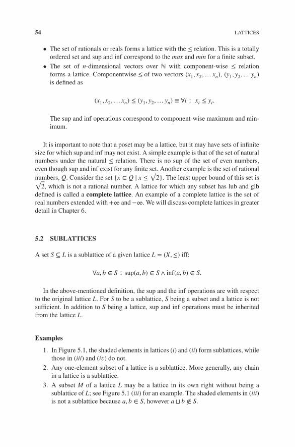
54 LATTICES
• The set of rationals or reals forms a lattice with the ≤ relation. This is a totallyordered set and sup and inf correspond to the max and min for a finite subset.
• The set of n-dimensional vectors over ℕ with component-wise ≤ relationforms a lattice. Componentwise ≤ of two vectors (x1, x2,… xn), (y1, y2,… yn)is defined as
(x1, x2,… xn) ≤ (y1, y2,… yn) ≡ ∀i ∶ xi ≤ yi.
The sup and inf operations correspond to component-wise maximum and min-imum.
It is important to note that a poset may be a lattice, but it may have sets of infinitesize for which sup and inf may not exist. A simple example is that of the set of naturalnumbers under the natural ≤ relation. There is no sup of the set of even numbers,even though sup and inf exist for any finite set. Another example is the set of rationalnumbers, Q. Consider the set {x ∈ Q | x ≤
√2}. The least upper bound of this set is√
2, which is not a rational number. A lattice for which any subset has lub and glbdefined is called a complete lattice. An example of a complete lattice is the set ofreal numbers extended with +∞ and −∞. We will discuss complete lattices in greaterdetail in Chapter 6.
5.2 SUBLATTICES
A set S ⊆ L is a sublattice of a given lattice L = (X,≤) iff:
∀a, b ∈ S ∶ sup(a, b) ∈ S ∧ inf(a, b) ∈ S.
In the above-mentioned definition, the sup and the inf operations are with respectto the original lattice L. For S to be a sublattice, S being a subset and a lattice is notsufficient. In addition to S being a lattice, sup and inf operations must be inheritedfrom the lattice L.
Examples
1. In Figure 5.1, the shaded elements in lattices (i) and (ii) form sublattices, whilethose in (iii) and (i𝑣) do not.
2. Any one-element subset of a lattice is a sublattice. More generally, any chainin a lattice is a sublattice.
3. A subset M of a lattice L may be a lattice in its own right without being asublattice of L; see Figure 5.1 (iii) for an example. The shaded elements in (iii)is not a sublattice because a, b ∈ S, however a ⊔ b ∉ S.

LATTICES AS ALGEBRAIC STRUCTURES 55
c
d
b
a
d
b c
a
b
d
a
c
d
a
b
c
(i) (ii)
(iii) (iv)
Figure 5.1 Examples: lattices and sublattices.
5.3 LATTICES AS ALGEBRAIC STRUCTURES
So far, we have looked at a lattice as a special type of poset, P = (X,≤) with ⊔ and ⊓
defined based on the ≤ relation.An alternative method of studying lattices is to start with a set equipped with the ⊔
and ⊓ operators and define ≤ relation based on these operations. Consider any set Xwith two algebraic operators ⊔ and ⊓. Assume that the operators satisfy the followingproperties:
(L1) a ⊔ (b ⊔ c) = (a ⊔ b) ⊔ c (associativity)
(L1)𝛿 a ⊓ (b ⊓ c) = (a ⊓ b) ⊓ c
(L2) a ⊔ b = b ⊔ a (commutativity)
(L2)𝛿 a ⊓ b = b ⊓ a
(L3) a ⊔ (a ⊓ b) = a (absorption)
(L3)𝛿 a ⊓ (a ⊔ b) = a.

56 LATTICES
a b c d e f ga a a ⊓ b a ⊓ c a ⊓ d a ⊓ e a ⊓ f a ⊓ gb b ⊔ a b b ⊓ c b ⊓ d b ⊓ e b ⊓ f b ⊓ gc c ⊔ a c ⊔ b c c ⊓ d c ⊓ e c ⊓ f c ⊓ gd d ⊔ a d ⊔ b d ⊔ c d d ⊓ e d ⊓ f d ⊓ ge e ⊔ a e ⊔ b e ⊔ c e ⊔ d e e ⊓ f e ⊓ gf f ⊔ a f ⊔ b f ⊔ c f ⊔ d f ⊔ e f f ⊓ gg g ⊔ a g ⊔ b g ⊔ c g ⊔ d g ⊔ e g ⊔ f g
Figure 5.2 Table notation for the algebra (X, ⊔, ⊓).
Theorem 5.2 Let (X, ⊔, ⊓) be a nonempty set with the operators ⊔ and ⊓ that satisfy(L1) − (L3) earlier. We define the operator ≤ on X by
a ≤ b ≡ (a ⊔ b = b).
Then,
• ≤ is reflexive, antisymmetric, and transitive
• sup(a, b) = a ⊔ b
• inf(a, b) = a ⊓ b.
Proof: Left as an exercise.
The algebra (X, ⊔, ⊓) can be represented by an n × n table, where |X| = n. It mayseem as though two n × n tables are needed, one for ⊔ and one for ⊓. However, asingle n × n table suffices, with one half used for ⊔ and the other for ⊓, as shown inFigure 5.2. By commutativity, a ⊔ b = b ⊔ a, and a ⊓ b = b ⊓ a, so populating bothhalves of the table for the same operation is redundant. In addition, by absorption,a ⊔ a = a ⊓ a = a, so the diagonal elements of the table agree for ⊔ and ⊓.
5.4 BOUNDING THE SIZE OF THE COVER RELATION OF A LATTICE
In this section, we give a bound on the number of edges in the cover relation of alattice. Consider a poset with n elements. Let ec be the number of edges in the coverrelation and e≤ be the number of edges in the poset relation.
Then, it is clear that ec ≤ e≤ ≤ n2. We prove that ec ≤ n3∕2.
Theorem 5.3 For a lattice L,
n − 1 ≤ ec ≤ n3∕2.
Proof: The lower bound is clear because every element in the lattice has at least onelower cover (except the smallest element). We show the upper bound.

JOIN-IRREDUCIBLE ELEMENTS REVISITED 57
Consider two distinct elements x, y ∈ L. Let B(x) denote the set of elements cov-ered by x. B(x)
⋂B(y) cannot have more than one element because that would violate
the lattice property. Let B′(x) = B(x)⋃{x}. Hence,
|B′(x)⋂
B′(y)| ≤ 1.
Let
L = {x0,… , xn−1},
bi = |B(xi)|.
Because there is no pair of elements in common between B′(x) and B′(y) for distinctx and y, we get
n−1∑
i=0
(bi + 1
2
)
≤
(n2
)
.
Simplifying, we getn−1∑
i=0
(b2i + bi) ≤ n2 − n.
Dropping bi from the left-hand side and −n from the right-hand side, we get
n−1∑
i=0
b2i < n2.
Since ec =∑
bi, we get
(ec
n
)2=(∑
bi
n
)2
≤
∑b2
i
n≤
n2
n= n.
The first inequality follows from Cauchy–Schwarz inequality.Therefore,
e2c ≤ n3.
5.5 JOIN-IRREDUCIBLE ELEMENTS REVISITED
We have defined join-irreducible elements of a poset in Chapter 1. Since latticesare posets with some additional properties, the same definition carries over. In fact,the concept of join-irreducible elements is more natural in the setting of latticeswhere the join operator between elements is always defined. In this section, we revisitjoin-irreducibles in lattices to show some of their useful properties. We use J(L) todenote the set of join-irreducible elements of lattice L.

58 LATTICES
: Join−irreducible elements
a b
d
c
Figure 5.3 Join-irreducible elements: J(L) = {a, b, c, d}.
For finite lattices, the elements with only one lower cover are join-irreducibleelements (see Problem 3).In the lattice shown in Figure 5.3, a, b, c, and d are join-irreducible. In a chain, allelements except the least element are join-irreducible.
In a finite Boolean lattice, the lattice of all subsets of a given finite set, only theatoms (elements that cover the bottom element) are join-irreducible.
We now show how join-irreducible elements help us reduce complexity of variousoperations. It is easily shown that for all posets:
a ≤ b ≡ ∀z ∶ z ≤ a ⇒ z ≤ b.
The advantage of the next lemma is that it only requires comparisons betweenjoin-irreducible elements and not all elements ≤ a.
Lemma 5.4 For a finite lattice L, a ≤ b is equivalent to ∀x ∶ x ∈ J(L) ∶ x ≤ a ⇒x ≤ b.
Proof: For the forward direction, a ≤ b and x ≤ a implies, for any x, x ≤ b by transi-tivity. For the reverse direction, denote by h(z) the height of z, i.e., the length (numberof edges) of the longest path from z to inf L in the cover graph (well-defined, since Lis a finite lattice). We will prove the property
P(a) ∶= ∀b ∶ ((∀x ∶ x ∈ J(L) ∶ x ≤ a ⇒ x ≤ b) ⇒ a ≤ b)
for all a ∈ L by strong induction on h(a). Given a, consider an arbitrary b and assume
(LHS) ∀x∶ x ∈ J(L)∶ x ≤ a ⇒ x ≤ b and (IH) P(c) holds for all c with h(c) < h(a).
(1) If h(a) = 0, then a = inf L ≤ b, and P(a) is vacuously true.(2) If a is join-irreducible, then, using x ∶= a in (LHS), a ≤ b follows, and P(a) isagain vacuously true.

PROBLEMS 59
(3) Now assume h(a) > 0 and a not join-irreducible. Then, there exist c ≠ a, d ≠ asuch that a = c ⊔ d. Since c ≠ a, we can conclude that h(a) ≥ h(c) + 1 (h measureslongest paths!). By (IH), P(c) holds, i.e., ∀b ∶ ((∀x ∶ x ∈ J(L) ∶ x ≤ c ⇒ x ≤ b) ⇒c ≤ b). We will use P(c) to show c ≤ b: assume x ∈ J(L) with x ≤ c, then x ≤ c ⊔ d =a, hence x ≤ a, thus, by (LHS), x ≤ b. Property P(c) delivers that c ≤ b. Similarly, onecan derive d ≤ b, hence c ⊔ d ≤ b, and with a = c ⊔ d, we obtain a ≤ b.
The following result strengthens the statement that a = ⊔x≤ax.
Lemma 5.5 For a finite lattice L and any a ∈ L,
a =⨆
{x ∈ J(L) ∶ x ≤ a}.
Proof: Let T = {x ∈ J(L) ∶ x ≤ a}. We have to show that a = lub(T).Since any x ∈ T satisfies x ≤ a, a is an upper bound on T . Consider any upper
bound u:
u is an upper bound on T≡ { Definition of upper bound }
x ∈ T ⇒ x ≤ u≡ { Definition of T }
(x ∈ J(L) ∧ x ≤ a) ⇒ x ≤ u≡ { Elementary propositional logic: (a ∧ b) ⇒ c ≡ a ⇒ (b ⇒ c) }
x ∈ J(L) ⇒ (x ≤ a ⇒ x ≤ u)≡ { Lemma 5.4 }
a ≤ u,
So, a is in fact the least upper bound on T .
Notice one special case: since a ∶= inf L is not considered join-irreducible, thelemma confirms that inf L =
⨆∅.
5.6 PROBLEMS
5.1. Show that a poset P = (X,≤) is a lattice iff for all finite subsets Y ⊆ X, sup Yand inf Y exist.
5.2. Show that the bound for ec can be improved when L is distributive, i.e., showthat if L is distributive then
ec ≤nlog2n
2.
5.3. Show that in finite lattices an element is join-irreducible iff it has only one lowercover.

60 LATTICES
5.7 BIBLIOGRAPHIC REMARKS
Most of the material in this chapter is quite standard and can be found in Birkhoff[Bir67], and Davey and Priestley [DP90]. The description of the bound on the size ofthe cover relation follows the reference Freese, Jaroslav, and Nation [FJN96].

6LATTICE COMPLETION
6.1 INTRODUCTION
We have seen that lattices are nicer structures than general posets because they allowus to take the meet and the join for any pair of elements in the set. What if we wantedto take the join and the meet of arbitrary subsets? Complete lattices allow us to doexactly that. All finite lattices are complete, so the concept of complete lattices isimportant only for infinite lattices. In this chapter, we first discuss complete latticesand show many ways in which complete lattices arise in mathematics and computerscience. In particular, topped ∩–structures and closure operators give us completelattices.
Next we consider the question: What if the given poset is not a complete lattice oreven a lattice? Can we embed it into a complete lattice? This brings us to the notionof lattice completion which is useful for both finite and infinite posets.
6.2 COMPLETE LATTICES
Recall the definition of a complete lattice.
Definition 6.1 (Complete Lattice) A poset P = (X,≤) is a complete lattice iff forall subsets Y ⊆ X, sup Y and inf Y exist.
Finite lattices are always complete. When X is infinite, then (X,≤) may be a latticebut not a complete lattice. Note that we require sup Y and inf Y to exist for all subsets
Introduction to Lattice Theory with Computer Science Applications, First Edition. Vijay K. Garg.© 2015 John Wiley & Sons, Inc. Published 2015 by John Wiley & Sons, Inc.
62 LATTICE COMPLETION
(not just finite subsets). For example, consider the set of natural numbers under theusual order. This poset is a lattice but not a complete lattice because sup is not definedfor subsets Y such as the set of all odd numbers. Note that in some cases, a latticecan be easily made complete by adding a few “artificial” elements. For example, wecan add a special element “∞” to the set of natural numbers. The set ℕ ∪ {∞} is acomplete lattice. It may not be enough to add finite number of elements to completea lattice. For example, the set of rationals with the elements ∞ and −∞ is not acomplete lattice. Consider the subset Y = {x ∈ X|x2 ≤ 2}. This set has no supremumin the set of rationals.
In the definition of complete lattices, note that when Y is the empty set, the require-ment that inf Y exist corresponds to existence of the ⊤ element. Similarly, when Y isthe empty set, sup Y equals the ⊥ element.
The following lemma provides us a way of showing that a lattice is complete byonly proving that the inf exists for any subset, saving us half the work.
Lemma 6.2 (Half-work Lemma) A poset P is a complete lattice iff inf S exists forevery S ⊆ P.
Proof: The forward direction (⇒) is easy.To show ⇐, we need to prove that sup S exists for every S. To do so, we will
formulate sup S in terms of the inf of some other set.Consider the set T of upper bounds of S, i.e.,
T = {x ∈ X | ∀s ∈ S ∶ s ≤ x}.
Now let a = inf T . We claim that a = sup S. From the definition of T , we get that∀s ∈ S ∶ ∀t ∈ T ∶ s ≤ t. Since a = inf T , it follows that ∀s ∈ S ∶ s ≤ a. Thus, a is anupper bound of S.
Further, for any upper bound t of S, we know that t ∈ T . Therefore, a ≤ t becausea = inf T . Thus, a = sup S.
Note that the set T in the proof may be empty. In that case, a would be the topelement of P.
6.3 CLOSURE OPERATORS
We find from experience that good structures tend to have multiple, equivalent waysof defining them. This is good for us in at least two ways. First, it provides multi-ple ways of characterizing the structure, hence offering us more flexibility in doingproofs. In addition, it may provide us efficient algorithms for dealing with the struc-tures. Here, we study two alternative definitions for complete lattices and then showtheir equivalence. The first definition is based on closure operators.
Given a set X, we denote the set of all subsets of X (the power set of X) by 2X . Wenow define closure operators on the set 2X .

TOPPED ∩–STRUCTURES 63
Definition 6.3 (Closure Operator) A map C ∶ 2X → 2X is a closure operator iff itsatisfies
1. ∀A ⊆ X,A ⊆ C(A) (increasing)
2. ∀A,B ⊆ X,A ⊆ B ⇒ C(A) ⊆ C(B) (monotone)
3. ∀A ⊆ X,C(C(A)) = C(A) (idempotent).
We now give some examples of the closure operator.
1. Given a poset P = (X,≤) and any subset Y ⊆ X, let
C(Y) = {x ∈ X | ∃y ∈ Y ∶ x ≤ y}.
C(Y) adds to Y all elements that are smaller than some element in Y . It is easyto verify that C is a closure operator.
2. Our next example is from the theory of formal languages. Let Σ be any alphabetand L ⊆ Σ∗ be a language (set of finite strings) defined over Σ. Then, Kleeneclosure of L consists of all finite strings that can be obtained by concatenationof strings in L. Thus, Kleene closure for a language L is defined as
C(L) = {x.y | x ∈ L ∧ y ∈ L},
where the operator . means concatenation. It is easy to verify that Kleene clo-sure satisfies all requirements of the closure operator.
Before we show the relationship between complete lattices and closure operators,we present yet another alternate definition, called topped ∩–structures.
6.4 TOPPED ∩–STRUCTURES
The second definition of a complete lattice is based on topped ∩–structures.
Definition 6.4 (Topped ∩–Structure) For a set X, let ⊆ 2X. is a topped∩–structure iff the following hold:
1. X ∈
2. [∀i ∈ I ∶ Ai ∈ ] ⇒ (⋂
i∈IAi ∈ ), where I is any indexing set.
Thus, a topped ∩–structure is a set of sets that contains the original set and isclosed under arbitrary intersection. From the Half-work Lemma, it is clear that topped∩–structures form a complete lattice under the relation ⊆.
We now show that closure operators are equivalent to topped ∩–structures.
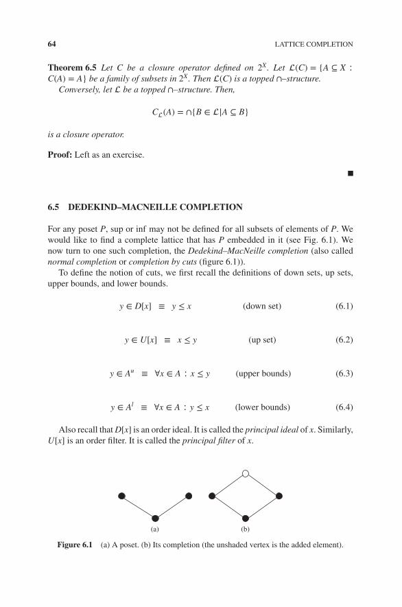
64 LATTICE COMPLETION
Theorem 6.5 Let C be a closure operator defined on 2X. Let (C) = {A ⊆ X ∶C(A) = A} be a family of subsets in 2X. Then (C) is a topped ∩–structure.
Conversely, let be a topped ∩–structure. Then,
C(A) = ∩{B ∈ |A ⊆ B}
is a closure operator.
Proof: Left as an exercise.
6.5 DEDEKIND–MACNEILLE COMPLETION
For any poset P, sup or inf may not be defined for all subsets of elements of P. Wewould like to find a complete lattice that has P embedded in it (see Fig. 6.1). Wenow turn to one such completion, the Dedekind–MacNeille completion (also callednormal completion or completion by cuts (figure 6.1)).
To define the notion of cuts, we first recall the definitions of down sets, up sets,upper bounds, and lower bounds.
y ∈ D[x] ≡ y ≤ x (down set) (6.1)
y ∈ U[x] ≡ x ≤ y (up set) (6.2)
y ∈ Au≡ ∀x ∈ A ∶ x ≤ y (upper bounds) (6.3)
y ∈ Al≡ ∀x ∈ A ∶ y ≤ x (lower bounds) (6.4)
Also recall that D[x] is an order ideal. It is called the principal ideal of x. Similarly,U[x] is an order filter. It is called the principal filter of x.
(a) (b)
Figure 6.1 (a) A poset. (b) Its completion (the unshaded vertex is the added element).
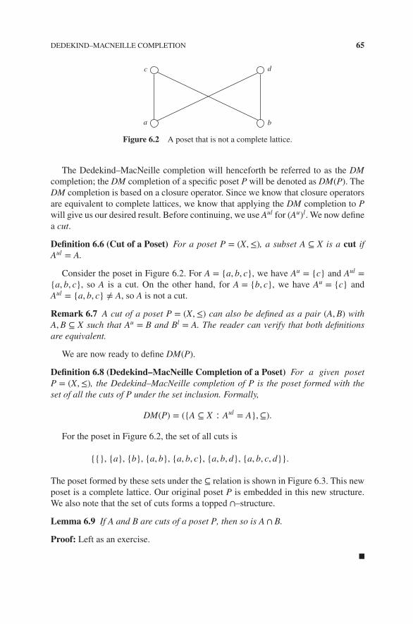
DEDEKIND–MACNEILLE COMPLETION 65
a
d
b
c
Figure 6.2 A poset that is not a complete lattice.
The Dedekind–MacNeille completion will henceforth be referred to as the DMcompletion; the DM completion of a specific poset P will be denoted as DM(P). TheDM completion is based on a closure operator. Since we know that closure operatorsare equivalent to complete lattices, we know that applying the DM completion to Pwill give us our desired result. Before continuing, we use Aul for (Au)l. We now definea cut.
Definition 6.6 (Cut of a Poset) For a poset P = (X,≤), a subset A ⊆ X is a cut ifAul = A.
Consider the poset in Figure 6.2. For A = {a, b, c}, we have Au = {c} and Aul ={a, b, c}, so A is a cut. On the other hand, for A = {b, c}, we have Au = {c} andAul = {a, b, c} ≠ A, so A is not a cut.
Remark 6.7 A cut of a poset P = (X,≤) can also be defined as a pair (A,B) withA,B ⊆ X such that Au = B and Bl = A. The reader can verify that both definitionsare equivalent.
We are now ready to define DM(P).
Definition 6.8 (Dedekind–MacNeille Completion of a Poset) For a given posetP = (X,≤), the Dedekind–MacNeille completion of P is the poset formed with theset of all the cuts of P under the set inclusion. Formally,
DM(P) = ({A ⊆ X ∶ Aul = A}, ⊆).
For the poset in Figure 6.2, the set of all cuts is
{{}, {a}, {b}, {a, b}, {a, b, c}, {a, b, d}, {a, b, c, d}}.
The poset formed by these sets under the ⊆ relation is shown in Figure 6.3. This newposet is a complete lattice. Our original poset P is embedded in this new structure.We also note that the set of cuts forms a topped ∩–structure.
Lemma 6.9 If A and B are cuts of a poset P, then so is A ∩ B.
Proof: Left as an exercise.
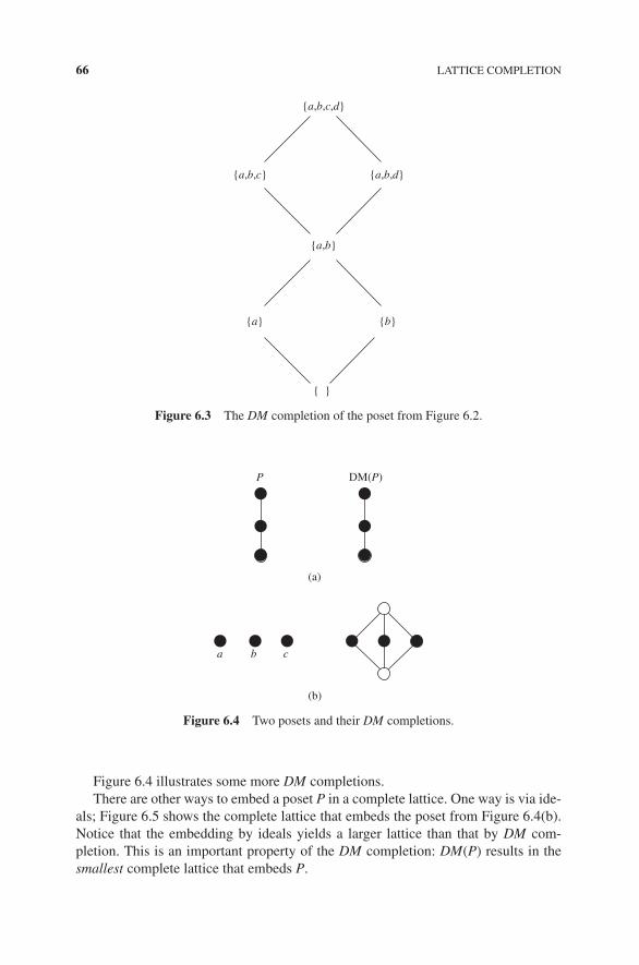
66 LATTICE COMPLETION
{ }
{a,b,c,d}
{a,b,c} {a,b,d}
{a,b}
{a} {b}
Figure 6.3 The DM completion of the poset from Figure 6.2.
DM(P)P
(a)
(b)
a b c
Figure 6.4 Two posets and their DM completions.
Figure 6.4 illustrates some more DM completions.There are other ways to embed a poset P in a complete lattice. One way is via ide-
als; Figure 6.5 shows the complete lattice that embeds the poset from Figure 6.4(b).Notice that the embedding by ideals yields a larger lattice than that by DM com-pletion. This is an important property of the DM completion: DM(P) results in thesmallest complete lattice that embeds P.

STRUCTURE OF DEDEKIND—MACNEILLE COMPLETION OF A POSET 67
{a,b,c}
{a,c}{a,b} {b,c}
{a} {b} {c}
{ }
Figure 6.5 The complete lattice via order ideals that embeds the poset from Figure 6.4(b).
6.6 STRUCTURE OF DEDEKIND—MACNEILLE COMPLETIONOF A POSET
In this section, we explore the structure of DM(P) for a poset P and exhibit a mappingthat show embedding of P into DM(P). We show calculational style of proofs in thissection. To facilitate such proofs, we give lemmas to eliminate or introduce inf andsup symbols as follows.
Lemma 6.10 Assuming inf A exists: x ≤ inf A ≡ ∀a ∈ A ∶ x ≤ a.
Lemma 6.11 Assuming sup A exists: x ≥ sup A ≡ ∀a ∈ A ∶ x ≥ a.
To manipulate formulae, it is also desirable to remove the “∀” symbols:
Lemma 6.12 (x ≤ y) ≡ (∀z ∶ z ≤ x ⇒ z ≤ y).
The forward direction holds due to transitivity ≤. The backward direction can beshown by substituting x for z and reflexivity of ≤ .
We are now ready to prove results about the structure of DM(P). We first showthat for any x ∈ P, D[x] is a cut and therefore belongs to DM(P).
Lemma 6.13 ∀x ∈ P ∶ D[x]ul = D[x].
Proof:We show that
D[x]u = U[x]. (6.5)
By duality:U[x]l = D[x]. (6.6)
Therefore, the result follows from (6.5) and (6.6). To prove (6.5): y ∈ D[x]u≡ {definition of upper bound as in (6.3)}∀z ∶ z ∈ D[x] ∶ z ≤ y

68 LATTICE COMPLETION
≡ {definition of D as in (6.1)}∀z ∶ z ≤ x ∶ z ≤ y
≡ {rules of predicate calculus}∀z ∶ z ≤ x ⇒ z ≤ y
≡ {property of ≤}x ≤ y
≡ {definition of U as in (6.2)}y ∈ U[x].
Therefore, D[x] is a map from P to DM(P). We now show that D[.] preserves allleast upper bounds and greatest lower bounds in P.
Lemma 6.14 Assume inf A exists. Then:⋂
∀a∈A
D[a] = D[inf A].
Proof: x ∈⋂
a∈A D[a]≡ {∩ = ∀ }∀a ∈ A ∶ x ∈ D[a]
≡ {definition of D as in (6.1)}∀a ∈ A ∶ x ≤ a
≡ {Lemma 6.10}x ≤ inf A
≡ {definition of D as in (6.1)}x ∈ D[inf A].
From lemmas 6.13 and 6.14, we know that there is a mapping from P to DM(P),which maps any element x ∈ P to D[x] that preserves the least upper bounds and thegreatest lower bounds. We next want to show that DM(P) contains only the elementsnecessary to complete P. To this end, we first define the notion of join-dense subsets.
Definition 6.15 (Join-Dense) Let P,Q be posets such that P ⊆ Q. P is join-dense inQ, if every element x ∈ Q is expressible as join of a subset A ⊆ P.
The notion of meet-dense can be defined dually.We now have the following theorem that characterizes Dedekind–MacNeille com-
pletion.
Theorem 6.16 Let P be any poset. Let f ∶ P → DM(P) be the order-embedding of Pinto DM(P) given by f (x) = D[x]. Then, f (P) is join-dense and meet-dense in DM(P).Moreover, if L is a complete lattice such that P is meet-dense and join-dense in L,then L is isomorphic to DM(P).
Proof: The proof is left as an exercise.

AN INCREMENTAL ALGORITHM FOR LATTICE COMPLETION 69
6.7 AN INCREMENTAL ALGORITHM FOR LATTICE COMPLETION
We now discuss algorithms for constructing DM completion of a poset.Let P be a poset and L be its Dedekind–MacNeille lattice completion. In this
section, we present an incremental algorithm for lattice completion in implicit rep-resentation in which both P and L are represented using vectors. Suppose that a newelement x is added to P with the constraint that x is not less than or equal to any of theexisting elements. Our goal is to compute the lattice completion, L′ of P′ = P ∪ {x}given P and L. When P is a singleton, then its completion is itself. By adding oneelement at a time in any linear order that is consistent with the partial order, we canuse the incremental algorithm for lattice completion of any poset.
Our incremental strategy for the lattice completion is as follows. We show that allthe elements of L other than the top element of L are also contained in L′. The topelement of L would be either retained or modified for L′. Therefore, except for thetop, our algorithm will simply add elements to L to obtain L′.
Lemma 6.17 Let S be a normal cut of P = (X,≤) such that S ≠ X. Then S is also anormal cut of P′ ∶= P ∪ {x} where x is a maximal element of P′.
Proof: Let T = Su in P. This implies that Tl = S in P because S is a normal cut of P.Since S ≠ X, T is nonempty (because if T is empty, Tl = X which is not equal to S).
If S ⊆ D[x], then Su in P′ equals T ∪ {x}. We need to show that Sul = S in P′, i.e.,(T ∪ {x})l = S in P′. The set (T ∪ {x})l = Tl ∩ D[x]. Since x is a maximal element,we know that x ∉ Tl. Since Tl = S and S ⊆ D[x], Tl ∩ D[x] = S. Hence, S is a normalcut of P′.
If S ⊈ D[x], then Su in P′ equals T . Since T is nonempty, and Tl = S in P, we getthat Tl = S in P′ as well. Hence, S is a normal cut of P′.
Our algorithm for DM construction is shown in Figure 6.6. Whenever a new ele-ment x arrives, we carry out three steps. In step 1, we process Y , the top element ofL; in step 2, we add a normal cut corresponding to the principal ideal of x; and, instep 3, we process the remaining elements of L. The goal of step 1 is to ensure thatL′ has a top element. The goal of step 2 is to ensure that all principal ideals of P′ arein L′. The goal of step 3 is to ensure that L′ is closed under intersection. In step 3, wefirst check if x covers more than one element. If it does not, then we do not have togo over all normal cuts in L because of the following claim.
Lemma 6.18 If x covers at most one element in P, then for any normal cut W ∈ L,min(W,D[x]) ∈ L assuming {} ∈ L.
Proof: If x does not cover any element of P, then D[x] = {x} and W ∩ D[x] = {},which is assumed to be in L. Now suppose that x covers just one element y, thenD[x] = {x} ∪ D[y]. Therefore, W ∩ D[x] = W ∩ D[y]. Since both W and D[y] are nor-mal cuts of L, so is W ∩ D[y].
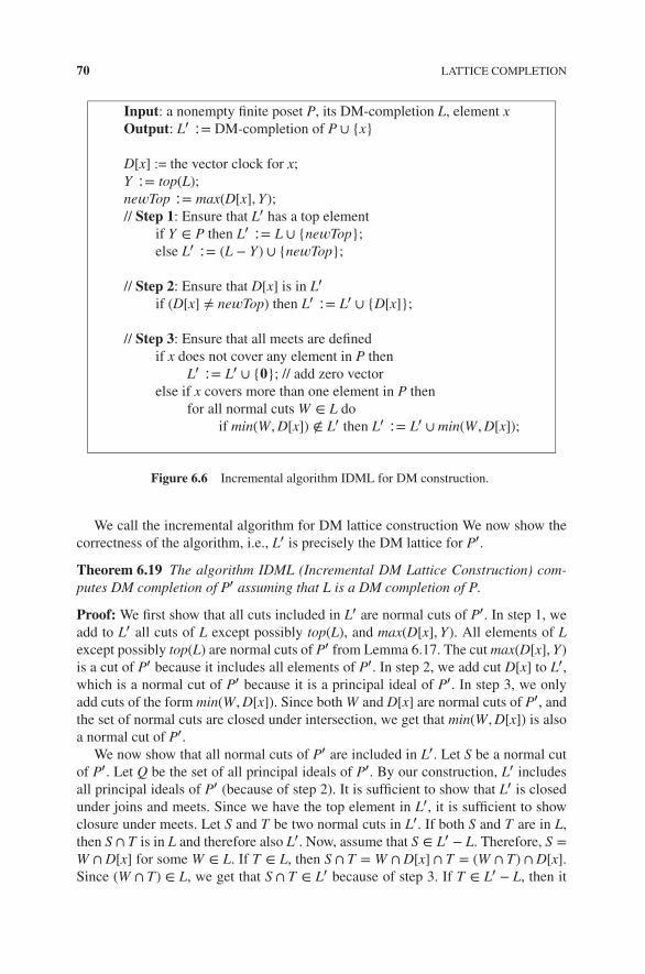
70 LATTICE COMPLETION
Input: a nonempty finite poset P, its DM-completion L, element xOutput: L′ ∶= DM-completion of P ∪ {x}
D[x] := the vector clock for x;Y ∶= top(L);ne𝑤Top ∶= max(D[x], Y);// Step 1: Ensure that L′ has a top element
if Y ∈ P then L′ ∶= L ∪ {ne𝑤Top};else L′ ∶= (L − Y) ∪ {ne𝑤Top};
// Step 2: Ensure that D[x] is in L′
if (D[x] ≠ ne𝑤Top) then L′ ∶= L′ ∪ {D[x]};
// Step 3: Ensure that all meets are definedif x does not cover any element in P then
L′ ∶= L′ ∪ {𝟎}; // add zero vectorelse if x covers more than one element in P then
for all normal cuts W ∈ L doif min(W,D[x]) ∉ L′ then L′ ∶= L′ ∪ min(W,D[x]);
Figure 6.6 Incremental algorithm IDML for DM construction.
We call the incremental algorithm for DM lattice construction We now show thecorrectness of the algorithm, i.e., L′ is precisely the DM lattice for P′.
Theorem 6.19 The algorithm IDML (Incremental DM Lattice Construction) com-putes DM completion of P′ assuming that L is a DM completion of P.
Proof: We first show that all cuts included in L′ are normal cuts of P′. In step 1, weadd to L′ all cuts of L except possibly top(L), and max(D[x], Y). All elements of Lexcept possibly top(L) are normal cuts of P′ from Lemma 6.17. The cut max(D[x], Y)is a cut of P′ because it includes all elements of P′. In step 2, we add cut D[x] to L′,which is a normal cut of P′ because it is a principal ideal of P′. In step 3, we onlyadd cuts of the form min(W,D[x]). Since both W and D[x] are normal cuts of P′, andthe set of normal cuts are closed under intersection, we get that min(W,D[x]) is alsoa normal cut of P′.
We now show that all normal cuts of P′ are included in L′. Let S be a normal cutof P′. Let Q be the set of all principal ideals of P′. By our construction, L′ includesall principal ideals of P′ (because of step 2). It is sufficient to show that L′ is closedunder joins and meets. Since we have the top element in L′, it is sufficient to showclosure under meets. Let S and T be two normal cuts in L′. If both S and T are in L,then S ∩ T is in L and therefore also L′. Now, assume that S ∈ L′ − L. Therefore, S =W ∩ D[x] for some W ∈ L. If T ∈ L, then S ∩ T = W ∩ D[x] ∩ T = (W ∩ T) ∩ D[x].Since (W ∩ T) ∈ L, we get that S ∩ T ∈ L′ because of step 3. If T ∈ L′ − L, then it

BREADTH FIRST SEARCH ENUMERATION OF NORMAL CUTS 71
can be written as W′ ∩ D[x] for some W′ ∈ L. Therefore, S ∩ T = W ∩ D[x] ∩ W ′ ∩D[x] = (W ∩ W′) ∩ D[x]. Since (W ∩ W ′) ∈ L, we again get that S ∩ T ∈ L′. SinceL′ contains all principal ideals of P′ and is closed under meet and join, we get that allnormal cuts of P′ are included in L′.
Note that our algorithm also gives an easy proof for the following claim.
Lemma 6.20 The number of normal cuts of P ∪ {x} is at most twice the number ofnormal cuts of P plus two.
Proof: For every cut in L, we add at most one more cut in step 3 of the algorithm.Further, we add at most one cut in step 1 and one additional cut in step 2.
We now discuss the time complexity of the IDML algorithm. Let m be the sizeof the lattice L. The time complexity of the IDML algorithm is dominated by step 3.Assuming that L is kept in a sorted order (for example, in the lexicographically sortedorder) in a binary balanced tree, the operation of checking whether min(W, S) ∈ L canbe performed in O(𝑤 log m), where 𝑤 is the width of the poset P′. For any elementfor which we traverse the lattice L, we take O(𝑤m log m) time. If the element x coversonly one element (or no elements), then we take O(𝑤 log m) time. Suppose that thereare r events in the poset that cover at least two events. In a distributed computation,only receive events would have this property. Then, to compute DM lattice of a posetP, we can repeatedly invoke IDML algorithm in any total order consistent with P.Therefore, we can construct DM lattice of a poset P of width 𝑤 with r elements oflower cover of size at least two in O(r𝑤m log m).
We also note here that given a poset P, to construct its DM-lattice, we can restrictour attention to its subposet of irreducible elements because DM-completion of Pis identical to DM-completion of the subposet containing all its join and meet irre-ducibles.
We have presented the algorithm based on computing closure under intersections.It is clear that by considering the complements of the sets, we can also construct thelattice via union closure. Formally, for poset P = (X,≤), let the basis IB be definedas
IB = {X − D[x]|x ∈ X}.
Let be defined as the family of sets obtained by taking union of some number ofsets in IB. We leave it as an exercise to show that ( , ⊇) is isomorphic to DM(P).
6.8 BREADTH FIRST SEARCH ENUMERATION OF NORMAL CUTS
In some distributed computing applications, we may be interested not in storing theDM lattice but simply enumerating all the elements of the lattice or storing onlythose elements of the lattice that satisfy a given property. Recall that the size of theDM-Lattice may be exponential in the size of the poset in the worst case. Algorithm

72 LATTICE COMPLETION
Input: a finite poset POutput: Breadth First Enumeration of elements of DM-completion of PG := bottom element ; := TreeSet of VectorClocks initially {G} with levelCompare order;
(1) while ( is notEmpty)(2) H := remove the smallest element from ;(3) output(H);(4) foreach event e enabled in H do;(5) K := the smallest normal cut containing Q ∶= H ∪ {e};(6) if K is not in , then add K to ;
int function levelCompare(VectorClock a, VectorClock b)(1) if (a.sum() > b.sum()) return 1;(2) else if (a.sum() < b.sum()) return -1;(3) for (int i = 0; i < a.size(); i++)(4) if (a[i] > b[i]) return 1;(5) if (a[i] < b[i]) return -1;(6) return 0;
Figure 6.7 Algorithm BFS-DML for BFS enumeration of DM-Lattice.
IDML has space complexity of O(m𝑤 log n) to store the lattice L (there are m ele-ments in the lattice, and each element is represented using a 𝑤-dimensional vector ofentries of size O(log n)). We now give an algorithm BFS-DML that does not requirestoring the entire lattice.
The algorithm BFS-DML views the lattice as a directed graph and generates itselements in the breadth first order. It is different from the traditional BFS algorithmon a graph because we do not store the graph or keep data that is proportional tothe size of the graph (such as the nodes already visited). Let Layer(k) be the set ofnodes in the graph that are at distance k from the bottom element of the lattice. Let𝑤L be the size of the largest set Layer(k). Then, the space required by BFS-DML isO(𝑤L𝑤 log n).
The algorithm BFS-DML is shown in Figure 6.7. The set is used to store the setof nodes that have been generated but have not been explored yet. The set is kept ina balanced binary tree so that it is easy to check if some element is already containedin the set. We maintain the invariant that the set contains only the normal cuts ofthe poset P. The elements in the binary search tree are compared using the functionlevelCompare shown in Figure 6.7. For any vector a corresponding to a consistentcut, the function a.sum() returns the number of events in the consistent cut. At lines(1) and (2) of the function levelCompare, we define a consistent cut to be smaller thanthe other if it has fewer elements. Lines (3)–(5) impose a lexicographic order on allconsistent cuts with equal number of elements. As a result, the function levelCompareimposes a total order on the set of all consistent and normal cuts.
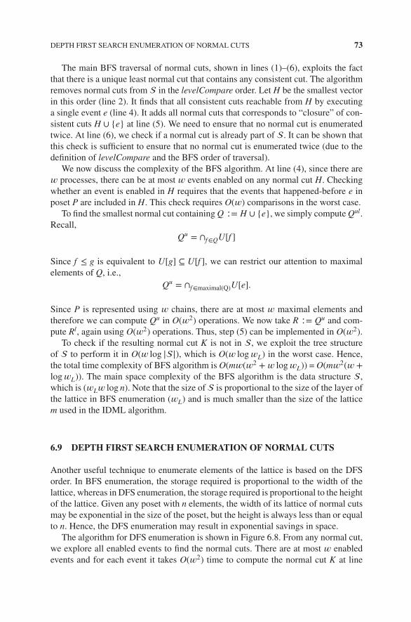
DEPTH FIRST SEARCH ENUMERATION OF NORMAL CUTS 73
The main BFS traversal of normal cuts, shown in lines (1)–(6), exploits the factthat there is a unique least normal cut that contains any consistent cut. The algorithmremoves normal cuts from in the levelCompare order. Let H be the smallest vectorin this order (line 2). It finds that all consistent cuts reachable from H by executinga single event e (line 4). It adds all normal cuts that corresponds to “closure” of con-sistent cuts H ∪ {e} at line (5). We need to ensure that no normal cut is enumeratedtwice. At line (6), we check if a normal cut is already part of . It can be shown thatthis check is sufficient to ensure that no normal cut is enumerated twice (due to thedefinition of levelCompare and the BFS order of traversal).
We now discuss the complexity of the BFS algorithm. At line (4), since there are𝑤 processes, there can be at most 𝑤 events enabled on any normal cut H. Checkingwhether an event is enabled in H requires that the events that happened-before e inposet P are included in H. This check requires O(𝑤) comparisons in the worst case.
To find the smallest normal cut containing Q ∶= H ∪ {e}, we simply compute Qul.Recall,
Qu = ∩f∈QU[f ]
Since f ≤ g is equivalent to U[g] ⊆ U[f ], we can restrict our attention to maximalelements of Q, i.e.,
Qu = ∩f∈maximal(Q)U[e].
Since P is represented using 𝑤 chains, there are at most 𝑤 maximal elements andtherefore we can compute Qu in O(𝑤2) operations. We now take R ∶= Qu and com-pute Rl, again using O(𝑤2) operations. Thus, step (5) can be implemented in O(𝑤2).
To check if the resulting normal cut K is not in , we exploit the tree structureof to perform it in O(𝑤 log ||), which is O(𝑤 log𝑤L) in the worst case. Hence,the total time complexity of BFS algorithm is O(m𝑤(𝑤2 +𝑤 log𝑤L)) = O(m𝑤2(𝑤 +log𝑤L)). The main space complexity of the BFS algorithm is the data structure ,which is (𝑤L𝑤 log n). Note that the size of is proportional to the size of the layer ofthe lattice in BFS enumeration (𝑤L) and is much smaller than the size of the latticem used in the IDML algorithm.
6.9 DEPTH FIRST SEARCH ENUMERATION OF NORMAL CUTS
Another useful technique to enumerate elements of the lattice is based on the DFSorder. In BFS enumeration, the storage required is proportional to the width of thelattice, whereas in DFS enumeration, the storage required is proportional to the heightof the lattice. Given any poset with n elements, the width of its lattice of normal cutsmay be exponential in the size of the poset, but the height is always less than or equalto n. Hence, the DFS enumeration may result in exponential savings in space.
The algorithm for DFS enumeration is shown in Figure 6.8. From any normal cut,we explore all enabled events to find the normal cuts. There are at most 𝑤 enabledevents and for each event it takes O(𝑤2) time to compute the normal cut K at line

74 LATTICE COMPLETION
Input: a finite poset P, starting state GOutput: DFS Enumeration of elements of DM-completion of P
(1) output(G);(2) foreach event e enabled in G do(3) K := smallest normal cut containing Q ∶= G ∪ {e};(4) M := get-Max-predecessor(K) ;(5) if M = G then(6) DFS-NormalCuts(K);
function VectorClock get-Max-predecessor(K) {//takes K as input vector and returns its maximum predecessor normal cut
(1) H = MinimalUpperBounds(K); // H ∶= Ku
(2) // find the maximal predecessor using normal cuts in the dual poset(3) foreach event f enabled in the cut H in Pd do(4) tempf := advance on event f in Pd from cut H;(5) // get the set of lower bounds on tempf
(6) pred := MaximalLowerBounds(tempf ) using Hl;(7) if (levelCompare(pred, maxPred) = 1) then maxPred = pred;(8) return maxPred;
Figure 6.8 Algorithm DFS-DML for DFS enumeration of DM-lattice.
(3). Since we are not storing the enumerated elements explicitly, we need a methodto ensure that the same normal cut is not visited twice.
Let pred(K) be the set of all normal cuts that are covered by K in the lattice. Weuse the total order levelCompare defined in Section 6.8 on the set pred(K). We makea recursive call on K from the normal cut G iff G is the maximum normal cut inpred(K) in the levelCompare order. Line (4) finds the maximum predecessor M usingthe traversal on the dual poset Pd. The dual of a poset P = (X,≤) is defined as follows.In the poset Pd, x ≤ y iff y ≤ x in P. It is easy to verify that S is a normal cut in P iff Su
is a normal cut in Pd. The function get-Max-Predecessor, shown in Figure 6.8, usesexpansion of a normal cut in the poset Pd to find the maximum predecessor. The func-tion get-Max-predecessor works as follows. At line (1), we compute H = Ku, whichis the normal cut in Pd corresponding to K. Our goal is to compute all predecessors ofK in P that corresponds to all successors of H in Pd. To find successors of H, we con-sider each event f enabled in H in Pd. At line (4), we compute the consistent cut tempf .The closure of tempf in Pd equals tempul
f in Pd. Equivalently, we can compute templuf
in P. The closed set templuf in Pd corresponds to the closed set templul
f in P. However,from Problem 4, we know that templul
f is equal to templf . Therefore, by computing
templf for each f enabled in H, we get all the predecessors of K in Pd. Since there can
be 𝑤 events enabled in H in Pd, and it takes O(𝑤2) time to compute each predecessor,it would take O(𝑤3) to determine the maximum predecessor. However, since tempf
and H differ on a single event, we can compute templf using Hl = K in O(𝑤) time. By

APPLICATION: FINDING THE MEET AND JOIN OF EVENTS 75
this observation, the complexity of computing max-predecessor reduces to O(𝑤2),and the total time complexity to determine whether K can be inserted is O(𝑤2).
In line (5) of DFS-DML, we traverse K using recursive DFS call only if M equalsG. Since the complexity of steps (3) and step (4) is O(𝑤2), the overall complexity ofprocessing a normal cut G is O(𝑤3) due to the foreach at line (2). Since there are mnormal cuts, we get the total time complexity of DFS-DML algorithm as O(m𝑤3).
The main space requirement of the DFS algorithm is the stack used for recursion.Every time the recursion level is increases, the size of the normal cut increases byat least 1. Hence, the maximum depth of the recursion is n. Therefore, the spacerequirement is O(n𝑤 log n) bits because we only need to store vectors of dimension𝑤 at each recursion level. Hence, the DFS algorithm takes significantly less spacethan the BFS algorithm.
6.10 APPLICATION: FINDING THE MEET AND JOIN OF EVENTS
Suppose that there are two events x and y on different processes that correspond tofaulty behavior. It is natural to determine the largest event, z, in the computation thatcould have affected both x and y. The event z is simply the meet of events x and y if itexists in the underlying computation. For example, in Figure 6.9(a), suppose that thefaulty events are {d, e}. In this case, the “root” cause of faults of these events couldbe event a. In the vector clock representation, the root cause is (1, 0, 0) in the DMlattice. Now consider the case when the set of faulty events is {e, f }. In this case, theunderlying computation does not have a unique maximum event that affects both eand f . It can be seen in Figure 6.9(a) that both the events b and c could be the “root”cause of the events e and f . This is exactly what we would get from the lattice ofnormal cuts. The largest normal cut that is smaller than both events e with vectorclock (1, 2, 1) and event f with vector clock (0, 1, 2) equals the vector (0, 1, 1), whichcorrectly identifies the set of events that affect both e and f .
d e f (2,0,0) (1,2,1) (0,1,2) (0,1,0)
(1,0,0)
(2,0,0) (1,2,1)
(2,2,2)
(0,1,2)
(0,1,1)
(0,0,1)
(1,0,0)
(a) (b) (c)
(0,1,0) (0,0,1) (0,0,0)a b c
Figure 6.9 (a) The original poset. (b) Equivalent representation using vector clocks. (c) ItsLattice of normal cuts.

76 LATTICE COMPLETION
Dual to the previous application, we may be interested in the smallest event zthat happened-after a subset of events. In a distributed system, an event z can havethe knowledge of event x only if x happened-before event z. If two events x and yhappened on different processes, we may be interested in the minimum event z thatknows about both x and y. In this case, z corresponds to the join of events x and y ifit exists in the underlying computation.
6.11 APPLICATION: DETECTING GLOBAL PREDICATES INDISTRIBUTED SYSTEMS
The key problem in detecting global predicates of a distributed computation is thatthe lattice of ideals (or consistent cuts) LI may be exponential in the size of the poset.The lattice of normal cuts, LDM, of a poset P is a suborder of the LI (every normal cutis consistent, but every consistent cut may not be normal). Its size always lies betweenthe size of the poset P and the size of the lattice of consistent cuts of P. In particular,it may be exponentially smaller than LI . We now show that a class of predicates canbe efficiently detected by traversing the lattice of normal cuts rather than LI .
The class of predicates we discuss are based on the idea of knowledge ina distributed system [HM84]. We define knowledge predicates based on thehappened-before relation. We use the notation G[i] to refer to events of G onprocess i.
Definition 6.21 Given a distributed computation, or equivalently a poset (P,≤), wesay that everyone knows the predicate B in the consistent cut G, if there exists aconsistent cut H such that H satisfies B and for every process i there exists an event ein G[i] such that all events in H happened before e. Formally, E(B,G) ≡ ∃H ∶ B(H) ∧∀i∃e ∈ G[i] ∶ ∀f ∈ H ∶ f ≤ e. We also define E(B) ≡ ∃G ∶ E(B,G).
Intuitively, the above-mentioned definition says that a predicate is known to every-one in the system if every process has a consistent cut in its past in which B was true.The definition captures the fact that in a distributed system, a process can know aboutremote events only through a chain of messages.
We now show that instead of traversing LI we can traverse LDM to detect E(B) forany global predicate B.
Theorem 6.22 Let B be any global predicate and G be a consistent cut such thatE(B,G). Then, there exists a normal cut N such that E(B,Nu).
Proof: Since everyone knows B in G, by the definition of “everyone knows,” we getthat there exists a consistent cut H ⊆ G such that B is true in H and every process inG knows H. Let be the set of all consistent cuts that know H. The set is nonemptybecause G ∈ . Furthermore, it is easy to show that the set is closed under inter-section. The least element K of the set corresponds to the minimal elements of thefilter Hu. Hence, we conclude that E(B,K).
Define N to be the consistent cut corresponding to Hul. It is clear that N is a nor-mal cut because it corresponds to the closure of H. Moreover, Nu = Hulu = Hu = K.

APPLICATION: DATA MINING 77
The first equality holds by the definition of N and the second equality holds due toproperties of u and l operators. Since K equals Nu, from E(B,K), we get that E(B,Nu).
6.12 APPLICATION: DATA MINING
Lattice theory has been used quite extensively for analysis of concepts in data miningapplications. Suppose that we have a set of objects G each of which has one or moreattributes from the set M. Can we automatically infer a concept from the knowledgeof which objects have which attributes? These concepts are studied in the branch ofmathematics called formal concept analysis which has many applications in datamining.
Definition 6.23 (Context) A context R is a triple (G,M, I), where G is the set ofobjects, M is the set of attributes, and I is the relation between G and M, i.e., I ⊆G × M.
Given any set of objects A ⊆ G, we can define the set of attributes common to allobjects in A as
Au = {m ∈ M|∀g ∈ A ∶ (g,m) ∈ I}
Similarly, given a set of attributes, B ⊆ M, we define the set of objects that all havethose attributes
Bl = {g ∈ G|∀m ∈ B ∶ (g,m) ∈ I}
.As an example, consider any poset P = (X,≤). We can treat this poset as a context
(X,X,≤), where the set of objects and attributes are X and the binary relation is theposet relation on P. Note that in this example, our notation for Au and Bl is consistentwith the definition of upper bounds (Au) and lower bounds (Bl) defined earlier.
Conversely, given a context (G,M, I), we can create a bipartite poset P = (X,≤)of height two with X as union of G and M and x ≤ y iff object x has attribute y.
We can now define a concept.
Definition 6.24 (Concept) A concept of a context R = (G,M, I) is a pair (A,B) suchthat Au = B and Bl = A.
For the context (X,X,≤) for any poset P = (X,≤), a concept is identical to thenormal cut of a poset.
We can put a partial order on the set of concepts as follows:
(A1,B1) ≤ (A2,B2)def= A1 ⊆ A2
It can be easily shown that A1 ⊆ A2 is equivalent to B1 ⊇ B2.

78 LATTICE COMPLETION
We have seen earlier that the set of normal cuts of P is a complete lattice DM(P)(the smallest complete lattice containing P). Similarly, the set of concepts form acomplete lattice (called the concept lattice) under the relation ≤ defined on concepts.
Given a context, by constructing DM completion of the poset corresponding to thecontext, we can generate the concept lattice.
6.13 PROBLEMS
6.1. Assume sup A exists in P. Show that
Aul = D[sup A].
6.2. Consider a poset (X,≤). Assume that for S ⊆ X , inf S exists. Let y = inf S. Showthat ∀x ∈ X ∶ x ≤ y ⇔ ∀s ∈ S ∶ x ≤ s.
6.3. Consider S,T ⊆ X, where X is a poset. Show that sup S ≤ inf T ⇒ ∀s ∈ S,∀t ∈T ∶ s ≤ t.
6.4. Show that for any subset A of a poset, Al = Alul and dually Au = Aulu.
6.5. Show that the completion of the set of rational numbers using cuts results in theset of real numbers.
6.6. Prove or disprove that every cut of a poset is also its order ideal.
6.7. Show that ( , ⊇) defined in Section 6.7 is isomorphic to DM(P).
6.8. Show that if A1 and A2 are cuts of a poset P, then so is A1 ∩ A2.
6.9. Prove Theorem 6.16.
6.14 BIBLIOGRAPHIC REMARKS
Most of the material in this chapter is quite standard and can be found in Davey andPriestley [DP90]. The main difference from the standard treatment is that we haveused calculational proofs for many of the results. Our discussion of algorithms forDM completion follows [Gar12].

7MORPHISMS
7.1 INTRODUCTION
In this chapter, we study homomorphisms between lattices. Many of the concepts andresults are analogous to those typically studied in group and ring theory. For example,the concept of lattice homomorphism is analogous to that of group homomorphism.These concepts have natural applications in the theory of distributed systems. In par-ticular, we show applications in predicate detection.
7.2 LATTICE HOMOMORPHISM
We begin by defining functions that preserve the order structure.
Definition 7.1 (Monotone function) Given two posets P = (X,≤P) and Q = (Y ,≤Q),a function f ∶ X → Y is called monotone iff
∀x, y ∈ X ∶ x ≤P y ⇒ f (x) ≤Q f (y)
The concept of preserving order can be extended to preserving meet and joinoperations.
Introduction to Lattice Theory with Computer Science Applications, First Edition. Vijay K. Garg.© 2015 John Wiley & Sons, Inc. Published 2015 by John Wiley & Sons, Inc.
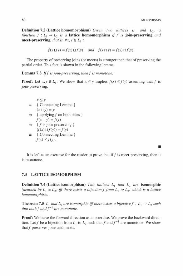
80 MORPHISMS
Definition 7.2 (Lattice homomorphism) Given two lattices L1 and L2, afunction f ∶ L1 → L2 is a lattice homomorphism if f is join-preserving andmeet-preserving, that is, ∀x, y ∈ L1 ∶
f (x ⊔ y) = f (x) ⊔ f (y) and f (x ⊓ y) = f (x) ⊓ f (y).
The property of preserving joins (or meets) is stronger than that of preserving thepartial order. This fact is shown in the following lemma.
Lemma 7.3 If f is join-preserving, then f is monotone.
Proof: Let x, y ∈ L1. We show that x ≤ y implies f (x) ≤ f (y) assuming that f isjoin-preserving.
x ≤ y≡ { Connecting Lemma }
(x ⊔ y) = y⇒ { applying f on both sides }
f (x ⊔ y) = f (y)⇒ { f is join-preserving }
(f (x) ⊔ f (y)) = f (y)≡ { Connecting Lemma }
f (x) ≤ f (y).
It is left as an exercise for the reader to prove that if f is meet-preserving, then itis monotone.
7.3 LATTICE ISOMORPHISM
Definition 7.4 (Lattice isomorphism) Two lattices L1 and L2 are isomorphic(denoted by L1 ≈ L2) iff there exists a bijection f from L1 to L2, which is a latticehomomorphism.
Theorem 7.5 L1 and L2 are isomorphic iff there exists a bijective f ∶ L1 → L2 suchthat both f and f−1 are monotone.
Proof: We leave the forward direction as an exercise. We prove the backward direc-tion. Let f be a bijection from L1 to L2 such that f and f−1 are monotone. We showthat f preserves joins and meets.
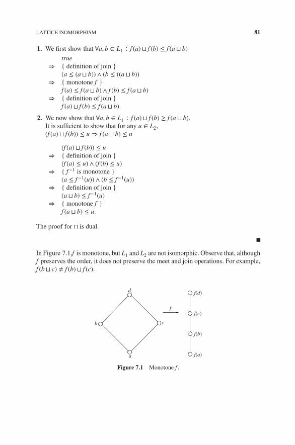
LATTICE ISOMORPHISM 81
1. We first show that ∀a, b ∈ L1 ∶ f (a) ⊔ f (b) ≤ f (a ⊔ b)true
⇒ { definition of join }(a ≤ (a ⊔ b)) ∧ (b ≤ ((a ⊔ b))
⇒ { monotone f }f (a) ≤ f (a ⊔ b) ∧ f (b) ≤ f (a ⊔ b)
⇒ { definition of join }f (a) ⊔ f (b) ≤ f (a ⊔ b).
2. We now show that ∀a, b ∈ L1 ∶ f (a) ⊔ f (b) ≥ f (a ⊔ b).It is sufficient to show that for any u ∈ L2,
(f (a) ⊔ f (b)) ≤ u ⇒ f (a ⊔ b) ≤ u
(f (a) ⊔ f (b)) ≤ u⇒ { definition of join }
(f (a) ≤ u) ∧ (f (b) ≤ u)⇒ { f−1 is monotone }
(a ≤ f−1(u)) ∧ (b ≤ f−1(u))⇒ { definition of join }
(a ⊔ b) ≤ f−1(u)⇒ { monotone f }
f (a ⊔ b) ≤ u.
The proof for ⊓ is dual.
In Figure 7.1,f is monotone, but L1 and L2 are not isomorphic. Observe that, althoughf preserves the order, it does not preserve the meet and join operations. For example,f (b ⊔ c) ≠ f (b) ⊔ f (c).
c
d
f
f(a)
f(b)
f(c)
f(d)
b
a
Figure 7.1 Monotone f .

82 MORPHISMS
7.4 LATTICE CONGRUENCES
Lattice homomorphisms can also be understood using the notion of lattice congru-ences. Informally, a congruence on a lattice (or any algebra) is an equivalence relationthat preserves lattice operations (operations of the algebra, respectively). Recall thata binary relation 𝜃 on a set X is an equivalence relation iff 𝜃 is reflexive, symmetric,and transitive.
The general structure of an equivalence relation is easy to understand because ofthe well-known correspondence between an equivalence relation and partitions of aset. An equivalence relation partitions a set into disjoint subsets called equivalenceclasses or blocks. A block [x]𝜃 consists of all elements in X that are related to x by therelation 𝜃. For example, consider the following relation on the set of natural numbers:
𝜃n = {(x, y)|x = y mod n} for n ≥ 1.
This relation partitions the set of natural numbers into n blocks. Conversely, given apartition of a set into a union of nonempty disjoint subsets, one can easily define anequivalence relation whose equivalence classes are the blocks in the partition.
An equivalence relation on a lattice L, which is compatible with both join and meetoperations is called a congruence on L. Formally,
Definition 7.6 (Lattice Congruence) An equivalence relation 𝜃 on a lattice L is acongruence iff for all x, y ∈ L, x ≡𝜃 y implies that
1. ∀z ∶ (z ⊔ x) ≡𝜃 (z ⊔ y)2. ∀z ∶ (z ⊓ x) ≡𝜃 (z ⊓ y).
The following lemma is left as an exercise.
Lemma 7.7 Let 𝜃 be a congruence of lattice L; then
1. (a ≡𝜃 b) ∧ (a ≤ c ≤ b)) ⇒ a ≡𝜃 c
2. a ≡𝜃 b iff (a ⊓ b) ≡𝜃 (a ⊔ b).
Example 7.8 Consider the lattice L with four elements {a, b, c, d} shown inFigure 7.1. Suppose we define an equivalence relation 𝜃 with two blocks {a, b} and{c, d}. It can be verified that 𝜃 is a lattice congruence. For example, c ≡𝜃 d impliesthat a ⊔ c and a ⊔ d are also equivalent under 𝜃.
Now consider another equivalence relation 𝛽 with three blocks {a, b}, {c}, and{d}.The relation 𝛽 is not a congruence because even though a and b are equivalentunder 𝛽, a ⊔ c, and b ⊔ c are not.

LATTICE HOMOMORPHISM AND CONGRUENCE 83
7.5 QUOTIENT LATTICE
Given a congruence 𝜃 on a lattice L, we can define quotient of L with respect to 𝜃 as
L∕𝜃 = {[a]𝜃|a ∈ L}.
The join and meet operations between the blocks of 𝜃 are defined naturally as
[a]𝜃 ⊔ [b]𝜃 = [a ⊔ b]𝜃.
Similarly,[a]𝜃 ⊓ [b]𝜃 = [a ⊓ b]𝜃.
The set L∕𝜃 together with the meet and join operations defined earlier is called thequotient lattice or the reduced lattice.
7.6 LATTICE HOMOMORPHISM AND CONGRUENCE
We now show that given a lattice homomorphism, one can define a lattice congruenceand vice versa.
Lemma 7.9 Let L and K be lattices and f ∶ L → K be a lattice homomorphism.Define the equivalence relation 𝜃 on L as follows: u ≡𝜃 𝑣 ⇐⇒ f (u) = f (𝑣). Then𝜃, called the kernel of f and denoted as ker f , is a congruence.
Proof: We need to show that if a ≡𝜃 b and c ≡𝜃 d then a ⊔ c ≡𝜃 b ⊔ d.
f (a ⊔ c)= { f is a lattice homomorphism }
f (a) ⊔ f (c)= { a ≡𝜃 b, c ≡𝜃 d }
f (b) ⊔ f (d)= { f is a lattice homomorphism }
f (b ⊔ d).
Therefore, a ⊔ c ≡𝜃 b ⊔ d. The proof for ⊓ is dual.
The following is a standard algebraic result.
Theorem 7.10 [Fundamental Homomorphism Theorem] Let L and K be lattices andf ∶ L → K be a lattice homomorphism. Define 𝜃 = ker f . The mapping g ∶ L∕𝜃 → Kgiven by g([a]𝜃) = f (a) is well defined and g is an isomorphism between L∕𝜃 and K.(Figure 7.2).
Proof: Left as an exercise.

84 MORPHISMS
L Kf
gq
L /θ
Figure 7.2 Fundamental Homomorphism Theorem.
a
c
(a) (b)
b
bd c
a
d
Figure 7.3 (a,b) Quadrilateral-closed structures.
7.7 PROPERTIES OF LATTICE CONGRUENCE BLOCKS
In this section, we explore the structure of a congruence block. We show that everycongruence block is a quadrilateral-closed convex sublattice. To this end, we firstdefine a quadrilateral in a lattice.
The elements a, b, c, and d in a lattice L form a quadrilateral < a, b; c, d > iff
1. a < b and c < d
2. (a ⊔ d = b) ∧ (a ⊓ d = c) or,(b ⊔ c = d) ∧ (b ⊓ c = a).
We say that a partition corresponding to 𝜃 is quadrilateral-closed if for everyquadrilateral < a, b; c, d >, we have that a ≡𝜃 b implies c ≡𝜃 d.
Theorem 7.11 An equivalence relation 𝜃 is a congruence iff
1. Each block of 𝜃 is a sublattice
2. Each block is convex
3. The blocks are quadrilateral-closed.

APPLICATION: MODEL CHECKING ON REDUCED LATTICES 85
Proof: First assume that 𝜃 is a congruence relation. We show the following.
1. Each block A of 𝜃 is a sublattice.We need to show that ∀a, b ∈ A ∶ (a ⊔ b ∈ A) ∧ (a ⊓ b ∈ A)
a ≡𝜃 b⇒ { take join with a }
a ⊔ a ≡𝜃 b ⊔ a≡ { join is idempotent }
a ≡𝜃 b ⊔ a.The proof for closure under the meet operation is similar.
2. Each block is convex.We show that ∀a, b ∈ A ∶ (a ≤ c ∧ c ≤ b) ⇒ c ∈ A
a ≡𝜃 b⇒ {taking join with c}
a ⊔ c ≡𝜃 b ⊔ c⇒ {a ≤ c, c ≤ b}
c ≡𝜃 b.3. The blocks are quadrilateral-closed.
It is sufficient to show that a ≡𝜃 b ⇒ c ≡𝜃 d, where < a, b; c, d > is a quadri-lateral.Assume that (a ⊔ d = b) ∧ (a ⊓ d = c). The proof when (b ⊔ c = d) ∧ (b ⊓ c =a) hold is similar. We are given that a ⊓ d = c. Moreover, since (a ⊔ d = b), weget that d ≤ b. Hence, b ⊓ d = d. Since a ⊓ d = c and b ⊓ d = d, we get thata ≡𝜃 b ⇒ c ≡𝜃 d (because 𝜃 is a congruence).The converse, i.e, conditions (1–3) imply that 𝜃 is a congruence class, is left asan exercise.
7.8 APPLICATION: MODEL CHECKING ON REDUCED LATTICES
We now show an application of congruences to checking temporal logic formulason Kripke structures (state transition graphs) that form a lattice. System propertiesand specifications are assumed to be expressed in temporal logic such as CTL−X(a restricted version of the computation tree logic (CTL), which does not have thenext-time operator X). The temporal logic formulas allow one to express properties onthe computation sequences (or paths) of the program. We do not deal with the struc-ture and semantics of the logic except to observe that formulas may make assertionson the paths in the state transition graphs.
One of the difficulties in mechanically checking a formula over a graph is thatthe number of states (or global states in a distributed system) may be prohibitivelylarge. One possible approach to alleviate this problem is to group together globalstates that have the same state with respect to the property that we wish to verify. Forexample, if we are interested in detecting the property of reaching a global state suchthat (x2 + y > 10), then it would simplify the problem of detection if we can group
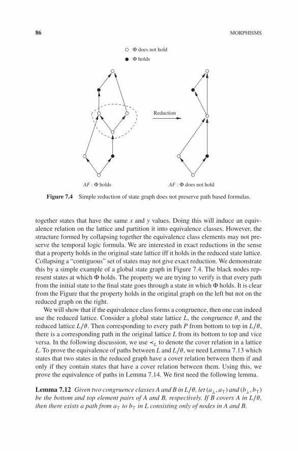
86 MORPHISMS
Φ does not hold
AF : Φ holds AF : Φ does not hold
Reduction
Φ holds
Figure 7.4 Simple reduction of state graph does not preserve path based formulas.
together states that have the same x and y values. Doing this will induce an equiv-alence relation on the lattice and partition it into equivalence classes. However, thestructure formed by collapsing together the equivalence class elements may not pre-serve the temporal logic formula. We are interested in exact reductions in the sensethat a property holds in the original state lattice iff it holds in the reduced state lattice.Collapsing a “contiguous” set of states may not give exact reduction. We demonstratethis by a simple example of a global state graph in Figure 7.4. The black nodes rep-resent states at which Φ holds. The property we are trying to verify is that every pathfrom the initial state to the final state goes through a state in which Φ holds. It is clearfrom the Figure that the property holds in the original graph on the left but not on thereduced graph on the right.
We will show that if the equivalence class forms a congruence, then one can indeeduse the reduced lattice. Consider a global state lattice L, the congruence 𝜃, and thereduced lattice L∕𝜃. Then corresponding to every path P from bottom to top in L∕𝜃,there is a corresponding path in the original lattice L from its bottom to top and viceversa. In the following discussion, we use ≺L to denote the cover relation in a latticeL. To prove the equivalence of paths between L and L∕𝜃, we need Lemma 7.13 whichstates that two states in the reduced graph have a cover relation between them if andonly if they contain states that have a cover relation between them. Using this, weprove the equivalence of paths in Lemma 7.14. We first need the following lemma.
Lemma 7.12 Given two congruence classes A and B in L∕𝜃, let (a⊥, a⊤) and (b⊥, b⊤)be the bottom and top element pairs of A and B, respectively. If B covers A in L∕𝜃,then there exists a path from a⊤ to b⊤ in L consisting only of nodes in A and B.

APPLICATION: MODEL CHECKING ON REDUCED LATTICES 87
Proof: Since B covers A in L∕𝜃, there exist elements c ∈ A and d ∈ B such thatc ≤ d in L. Since c ≤ a⊤, we get that c ≤ d ⊓ a⊤ ≤ a⊤. From convexity of A, weget that d ⊓ a⊤ ∈ A. Consider the quadrilateral < d ⊓ a⊤, a⊤; d, d ⊔ a⊤ >. From thequadrilateral-closed property of congruences, we get that d ⊔ a⊤ ∈ B. This impliesthat d ⊔ a⊤ ≤ b⊤. Therefore a⊤ ≤ b⊤. Hence, there exists a path from a⊤ to b⊤ in L.
It remains to be shown that the path consists only of nodes belonging to A or B.Pick any e ∈ L such that it is on the path from a⊤ to b⊤. Thus, a⊤ ≤ e ≤ b⊤ and sinceA ≺L∕𝜃 B, hence by property of the covering relation either e ∈ A or e ∈ B, whichyields the desired result.
Lemma 7.13 Let A, B ∈ L∕𝜃, then
A ≺L∕𝜃 B
iff there exist m, n ∈ L such that
n ∈ A, m ∈ B and n ≺L m.
Proof: The forward direction of the proof follows from Lemma 7.12 as follows: Weassume that A ≺L∕𝜃 B. Thus, by Lemma 7.12, there exists a path from a⊤ to b⊤ in Lconsisting only of nodes in A and B. The first element in the path is a⊤ and let thesecond element on the path be b. Clearly b ∈ B and a⊤ ≺L b. Thus, there exist m,n ∈ L such that n ∈ A, m ∈ B and n ≺L m.
To prove the converse, we assume that A, B ∈ L∕𝜃 and there exist m, n ∈ L suchthat n ∈ A, m ∈ B and n ≺L m. Let us assume that there exists C ∈ L∕𝜃 such thatA <L∕𝜃 C ≺L∕𝜃 B (Figure 7.5).
Because n ≺L m, we cannot have n ≤ c⊤ ≤ m (from the definition of cover rela-tion). Thus ¬(c⊤ ≤ m). (Figure 7.5(b)). Since C ≺L∕𝜃 B, c⊤ < b⊤ from Lemma 7.12.Therefore, ¬(m ≤ c⊤) (otherwise, m ≤ c⊤ ≤ b⊤ implies c⊤ ∈ B due to convexity).Hence, m ∥ c⊤.
Since n ≺L m, m ∥ c⊤, and n ≤ c⊤, it follows that m ⊓ c⊤ = n. It can be now veri-fied that < m,m ⊔ c⊤; n, c⊤ > forms a quadrilateral in L.
Now we show that m ⊔ c⊤ ∈ B. This follows from convexity of B because m ≤
m ⊔ c⊤ ≤ b⊤.Since m ⊔ c⊤ ≡𝜃 m, hence from the quadrilateral-closed property of congruences
we have, n ≡𝜃 c⊤. Therefore, c⊤ ∈ A. This contradicts our assumption that thereexists C ∈ L∕𝜃 such that A <L∕𝜃 C ≺L∕𝜃 B.
Now we can prove that there is a one-to-one correspondence between paths ofL and L∕𝜃. The first part of the lemma says that for any path in L∕𝜃, if we lookat the preimages of the nodes on the path (corresponding to inverse of the latticehomomorphism function f ), then there exists a subset of these preimage nodes, which

88 MORPHISMS
A
B
bTb
aa
b⊥
a⊥ a⊥
b⊥
n
m m
L /θ
L
C
A
B
n
C
m c
c c
c⊥ c⊥
L /θ
L
<L /θ <L /θ
(a) (b)
⊥
⊥
⊥ ⊥
⊥
⊥
Figure 7.5 (a,b) Proof of Lemma 7.13
also forms a path in L. Since f is defined to preserve values of variables relevant tothe property being detected, this enables us to prove that detecting temporal formulain L is equivalent to detecting temporal formulae in L∕𝜃. Similarly, the second partof the lemma proves that for every path in L, if we look at the image of the nodes onthe path, then they form a corresponding path in L∕𝜃.
Lemma 7.14 [Equivalence of Paths] Let f be the lattice homomorphism correspond-ing to 𝜃.
1. If P = (P1, ...,Pk) is a path from bottom to top in L∕𝜃, then there exists a pathQ in L such that Q ⊆ {q ∈ L ∶ ∃i ∈ [1, k] ∶ q ∈ f−1(Pi)}.
2. If Q = (q1, ..., qk) is a path from bottom to top in L, then the set P ={f (q1), ..., f (qk)} forms a path from bottom to top in L∕𝜃 (Figure 7.6 illustratesthe lemma).
Proof:
1. Consider the set f−1(Pi). For any i ∈ [1, k], let xi and yi be the bottom and topelements of f−1(Pi), respectively (f−1(Pi), is a sublattice). Note that x1 and ykare the bottom and top elements of L. From Lemma 7.12, we get that there is apath from y1 → y2 → ... → yk. In addition, since f−1(P1) is a sublattice, hencethere is a path x1 → y1. Therefore, there is a path from x1 (bottom) to yk (top)in L.
2. Let f (qi,1), ..., f (qi,l) be the sequence obtained from P after removing dupli-cate nodes. From the definition of f (qi,k) and f (qi,k+1), there exists m, n ∈ Lsuch that m ∈ f (qi,k), n ∈ f (qi,k+1) and m ≺L n. Then Lemma 7.13 gives us
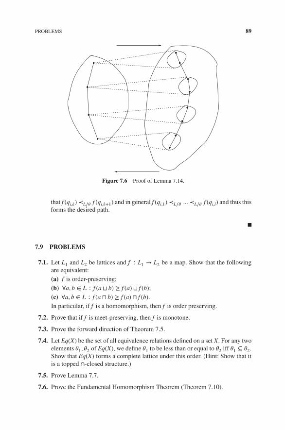
PROBLEMS 89
Figure 7.6 Proof of Lemma 7.14.
that f (qi,k) ≺L∕𝜃 f (qi,k+1) and in general f (qi,1) ≺L∕𝜃 ... ≺L∕𝜃 f (qi,l) and thus thisforms the desired path.
7.9 PROBLEMS
7.1. Let L1 and L2 be lattices and f ∶ L1 → L2 be a map. Show that the followingare equivalent:(a) f is order-preserving;
(b) ∀a, b ∈ L ∶ f (a ⊔ b) ≥ f (a) ⊔ f (b);(c) ∀a, b ∈ L ∶ f (a ⊓ b) ≥ f (a) ⊓ f (b).In particular, if f is a homomorphism, then f is order preserving.
7.2. Prove that if f is meet-preserving, then f is monotone.
7.3. Prove the forward direction of Theorem 7.5.
7.4. Let Eq(X) be the set of all equivalence relations defined on a set X. For any twoelements 𝜃1, 𝜃2 of Eq(X), we define 𝜃1 to be less than or equal to 𝜃2 iff 𝜃1 ⊆ 𝜃2.Show that Eq(X) forms a complete lattice under this order. (Hint: Show that itis a topped ∩-closed structure.)
7.5. Prove Lemma 7.7.
7.6. Prove the Fundamental Homomorphism Theorem (Theorem 7.10).

90 MORPHISMS
7.7. Complete the proof of Theorem 7.11.
7.8. ([CG06]) Show that a formula 𝜙 in temporal logic CTL−X holds in L iff it holdsin L∕𝜃, where 𝜃 is the congruence class corresponding to all nontemporal sub-formulas in 𝜙.
7.10 BIBLIOGRAPHIC REMARKS
The discussion on lattice homomorphisms and congruence lattices is quite standard.The reader is referred to Grätzer [Grä03] for various proofs. The application of latticecongruences to model checking is taken from Chakraborty and Garg [CG06].

8MODULAR LATTICES
8.1 INTRODUCTION
We describe a special class of lattices called modular lattices. Modular lattices arenumerous in mathematics; for example, the lattice of normal subgroups of a groupis modular, the lattice of ideals of a ring is modular, and so is the finite-dimensionalvector space lattice. Distributive lattices are a special class of modular lattices. Theset of all consistent global states in a distributed computation forms a distributivelattice and is therefore a modular lattice.
In this chapter, we first introduce both modular and distributive lattices to show therelationship between them. Later, we focus on modular lattices. Distributive latticesare considered in detail in Chapter 9.
8.2 MODULAR LATTICE
Definition 8.1 (Modular Lattice) L is modular if ∀a, b, c ∈ L ∶ a ≥ c ⇒ a ⊓ (b ⊔
c) = (a ⊓ b) ⊔ c.
The definition says that if c ≤ a, then one can bracket the expression a ⊓ b ⊔ c eitherway.
We will show that all distributive lattices are modular. Recall that a lattice L isdistributive if ∀a, b, c ∶ a ⊓ (b ⊔ c) = (a ⊓ b) ⊔ (a ⊓ c).
Introduction to Lattice Theory with Computer Science Applications, First Edition. Vijay K. Garg.© 2015 John Wiley & Sons, Inc. Published 2015 by John Wiley & Sons, Inc.

92 MODULAR LATTICES
In this definition, the equality can be replaced by ≤ because of the following obser-vation.
Lemma 8.2 For all lattices, a ⊓ (b ⊔ c) ≥ (a ⊓ b) ⊔ (a ⊓ c).
Proof: We know that
1. a ⊓ (b ⊔ c) ≥ (a ⊓ b)2. a ⊓ (b ⊔ c) ≥ (a ⊓ c)
Combining (1) and (2), we get
a ⊓ (b ⊔ c) ≥ (a ⊓ b) ⊔ (a ⊓ c).
A similar observation applies to the definition of modular lattices as shown by thefollowing lemma.
Lemma 8.3 For all lattices, a ≥ c ⇒ a ⊓ (b ⊔ c) ≥ (a ⊓ b) ⊔ c.
Proof: a ≥ c ⇒ (a ⊓ c) = c
Using Lemma 8.2 it follows that a ⊓ (b ⊔ c) ≥ (a ⊓ b) ⊔ c.
We can now show the relationship between the modularity condition and the distribu-tivity condition for lattices.
Theorem 8.4 L is distributive implies that L is modular.
Proof: L is distributive≡ { definition of a distributive lattice }
∀a, b, c ∶ a ⊓ (b ⊔ c) = (a ⊓ b) ⊔ (a ⊓ c)⇒ { a ≥ c is equivalent to a ⊓ c = c }
∀a, b, c ∶ a ≥ c ⇒ a ⊓ (b ⊔ c) = (a ⊓ b) ⊔ c≡ { definition of a modular lattice }
L is modular.
8.3 CHARACTERIZATION OF MODULAR LATTICES
We now give examples of lattices that are not modular or modular but not distributive.All lattices of four elements or less are modular. The smallest lattice which is not

CHARACTERIZATION OF MODULAR LATTICES 93
modular is the pentagon (N5) shown in Figure 1.4(a). In this lattice, a ≥ c holds;however, a ⊓ (b ⊔ c) = a ⊓ 1 = a, whereas (a ⊓ b) ⊔ c = 0 ⊔ c = c.
The diamond lattice (M3) shown in Figure 1.4(b) is modular but not distributive. Tosee this, note that in the diagram of M3 we have
a ⊓ (b ⊔ c) = a ⊓ 1 = a
and (a ⊓ b) ⊔ (a ⊓ c) = 0 ⊔ 0 = 0.
Since a ≠ 0, M3 is not distributive.
We now focus on modular lattices and list some theorems that characterize modularlattices.
In the definition of modular lattices, if c satisfies (a ⊓ b) ≤ c ≤ a, then we get thata ⊓ (b ⊔ c) = (a ⊓ b) ⊔ c = c. The following theorem shows that to check modularityit is sufficient to consider c’s that are in the interval [a ⊓ b, a].
Theorem 8.5 A lattice L is modular iff ∀a, b ∈ L
d ∈ [a ⊓ b, a] ⇒ a ⊓ (b ⊔ d) = d. (8.1)
Proof:
First, we show that (8.1) implies that L is modular, i.e.,
∀a, b, c ∈ L ∶ a ≥ c ⇒ a ⊓ (b ⊔ c) = (a ⊓ b) ⊔ c.
When c ≤ a and a ⊓ b ≤ c, we get that a ⊓ (b ⊔ c) = (a ⊓ b) ⊔ c because the left-handside equals c from (8.1) and the right-hand side equals c because (a ⊓ b) ≤ c.
Now suppose c ≤ a but a ⊓ b ≤ c is false (see Figure 8.1). We define d = (a ⊓ b) ⊔ c.Clearly d ∈ [a ⊓ b, a].
Consider a ⊓ (b ⊔ d). Replacing the value of d in (8.1) we get
a ⊓ (b ⊔ ((a ⊓ b) ⊔ c)) = (a ⊓ b) ⊔ c. (8.2)
a b
d
ca b
Figure 8.1 Proof of Theorem 8.5.

94 MODULAR LATTICES
Now consider a ⊓ (b ⊔ c). Using the fact that c ≤ (a ⊓ b) ⊔ c we get
a ⊓ (b ⊔ c) ≤ a ⊓ (b ⊔ ((a ⊓ b) ⊔ c)). (8.3)
Combining (8.2) and (8.3), we get a ⊓ (b ⊔ c) ≤ (a ⊓ b) ⊔ c.
Since a ⊓ (b ⊔ c) ≥ (a ⊓ b) ⊔ c holds for all lattices (Lemma 8.3), we get
a ⊓ (b ⊔ c) = (a ⊓ b) ⊔ c.
Hence, L is modular.
Showing the other side, that modularity implies condition (8.1) is trivial and is left asan exercise.
The following lemma is useful in proving the Pentagon theorem, which gives a char-acterization of modular lattices using the absence of a sublattice isomorphic to apentagon (or N5).
Lemma 8.6 For all lattices L, consider any a, b, c ∈ L. Let 𝑣 = a ⊓ (b ⊔ c)) and u =(a ⊓ b) ⊔ c. Thus, 𝑣 and u are expressions obtained by different bracketing of theexpression a ⊓ b ⊔ c. Then,
1. 𝑣 > u ⇒ (𝑣 ⊓ b) = (u ⊓ b).2. 𝑣 > u ⇒ (𝑣 ⊔ b) = (u ⊔ b).
Proof: We show the first assertion. The proof for the second one is similar.a ⊓ b
=(a ⊓ b) ⊓ b
≤
[(a ⊓ b) ⊔ c)] ⊓ b= { definition of u }
u ⊓ b≤ { 𝑣 > u }
𝑣 ⊓ b= { definition of 𝑣 }
(a ⊓ (b ⊔ c)) ⊓ b= { b ≤ b ⊔ c }
a ⊓ b.
The above-mentioned sequence of inequalities implies that all the intermediateexpressions must be equal; therefore, u ⊓ b = 𝑣 ⊓ b.

CHARACTERIZATION OF MODULAR LATTICES 95
We are now ready for another characterization of modular lattices due to R. Dedekind.
Theorem 8.7 [Pentagon Theorem] A lattice L is modular iff it does not contain asublattice isomorphic to N5.
Proof: If L contains N5, then it clearly violates modularity as shown earlier. Nowassume that L is not modular. Then, there exist a, b, c such that a > c and a ⊓ (b ⊔ c) >(a ⊓ b) ⊔ c. It can be verified that b||a and b||c. For example, b ≤ a implies (a ⊓ b) ⊔c = b ⊔ c ≤ a ⊓ (b ⊔ c). The other cases are similar.
We let 𝑣 = a ⊓ (b ⊔ c) and u = (a ⊓ b) ⊔ c). We know that 𝑣 > u. It is easy to verifythat b||u and b||𝑣. For example, b < 𝑣 ≡ b < a ⊓ (b ⊔ c) ⇒ (b < a).
From Lemma 8.6, u ⊔ b = 𝑣 ⊔ b and u ⊓ b = 𝑣 ⊓ b.
Thus, u, 𝑣, b, u ⊔ b, and u ⊓ b form N5.
Modular lattices can also be characterized using an identity on lattices. An advan-tage of a characterization based on identities is that it allows easy manipulation ofexpressions: the left-hand side of any identity can be replaced by the right-hand side.
Theorem 8.8 A lattice L is modular iff ∀a, b, c ∈ La ⊓ (b ⊔ (a ⊓ c)) = (a ⊓ b) ⊔ (a ⊓ c).
Proof: Substitute (a ⊓ c) for c in the definition 8.1.
Consider two incomparable elements a and b as shown in Figure 8.2. Define twointervals [a, a ⊔ b], and [a ⊓ b, b]. We can define maps f and g from one interval tothe other as follows.
f ∶ x → x ⊓ b
g ∶ y → y ⊔ a.
Theorem 8.9 [Diamond Isomorphism Theorem] A lattice L is modular iff ∀a, b ∶ fand g as defined earlier are isomorphic.
Proof: First we show that modularity implies f and g are isomorphic. In order to showthat f and g are isomorphic, we need to show that
1. f and g are homomorphic.
2. they are bijective.

96 MODULAR LATTICES
a bg
f
a b
a b
Figure 8.2 Theorem 8.9.
In order to show f is a lattice homomorphism, we show that it is join preserving andmeet preserving.
We first show that f is join preserving, that is, f (x1 ⊔ x2) = f (x1) ⊔ f (x2). Consider theright-hand side
f (x1) ⊔ f (x2)
= (x1 ⊓ b) ⊔ (x2 ⊓ b)
= x2 ⊓ b {x1 ≤ x2}
Now taking the left-hand side, we get
f (x1 ⊔ x2)
= (x1 ⊔ x2) ⊓ b
= x2 ⊓ b. {x1 ≤ x2}.
Hence, f is join preserving. It can be shown similarly that f is also meet preserving.Similarly, g preserves both join and meet. Hence, f and g are lattice homomorphisms.
We now show that f and g are inverses of each other. Consider
f ∘g(x)
= g(f (x))
= (x ⊓ b) ⊔ a
= x ⊓ (b ⊔ a) from modularity
= x.
Therefore f = g−1. Hence, f and g are bijective. This concludes our proof that f andg are lattice isomorphisms. We leave it as an exercise to show the converse.

CHARACTERIZATION OF MODULAR LATTICES 97
We now give yet another characterization of modular lattices using upper and lowercovering conditions.
Definition 8.10 (Upper Covering Condition) A lattice L satisfies the Upper Cov-ering Condition iff
∀x, y, z ∈ L ∶ x <c y ⇒ (x ⊔ z) <c (y ⊔ z). The Lower Covering Condition is dual.
Theorem 8.11 A lattice L is modular iff it satisfies the Upper Covering Conditionand the Lower Covering Condition.
Proof: We leave this proof as an exercise in using the Diamond IsomorphismTheorem.
We now define a ranked poset and a graded poset. Some examples are shown inFigure 8.3.
Definition 8.12 (Ranked poset) A poset is ranked if there exists a ranking functionr ∶ P → N such that r(x) = r(y) + 1 whenever x covers y.
Definition 8.13 (Graded poset) A ranked poset is graded if all maximal chains havethe same length.
(b)
(c)
(a)
(d)
Figure 8.3 (a) A ranked poset, (b) A poset that is not ranked, (c) A ranked and graded poset,and (d) A ranked and graded lattice.

98 MODULAR LATTICES
Theorem 8.14 A lattice L is modular iff L is graded and the ranking function satisfies
r(x) + r(y) = r(x ⊓ y) + r(x ⊔ y).
Proof: The proof of the theorem is left as an exercise.
8.4 PROBLEMS
8.1. Show that if L is a graded lattice, then
(a) r(x) + r(y) ≥ r(x ⊓ y) + r(x ⊔ y) is equivalent to the Upper Covering Condi-tion.
(b) r(x) + r(y) ≤ r(x ⊓ y) + r(x ⊔ y) is equivalent to the Lower Covering Con-dition.
8.2. Complete the proof of Theorem 8.5.
8.3. Show the shearing identity for modular lattices.[Shearing Identity] A lattice L is modular iff ∀x, y, z ∶ x ⊓ (y ⊔ z) = x ⊓ ((y ⊓(x ⊔ z)) ⊔ z).
8.4. Complete the proof of Theorem 8.9.
8.5. Prove Theorem 8.11.
8.6. Prove Theorem 8.14.
8.5 BIBLIOGRAPHIC REMARKS
The book by Gratzer [Grä71, Grä03] contains most of the results in this chapter exceptfor our emphasis on calculational proofs.

9DISTRIBUTIVE LATTICES
9.1 INTRODUCTION
Recall that a lattice L is distributive if
∀a, b, c ∈ L ∶ a ⊓ (b ⊔ c) = (a ⊓ b) ⊔ (a ⊓ c). (9.1)
Distributive lattices form one of the most interesting class of lattices. Many latticesthat arise in distributed computing and combinatorics are distributive. The set of allconsistent global states in a distributed computation forms a distributive lattice. Theset of all subsets of any set forms a distributive lattice under the subset relation.
In this chapter, we discuss some of the crucial properties of distributive lattices.Section 9.2 gives a characterization of distributive lattices using forbidden sublat-tices. In Section 9.4, we discuss a duality between finite distributive lattices andfinite posets. Every finite distributive lattice can be recovered from the poset of itsjoin-irreducible elements. This result due to Birkhoff,is known as the fundamentaltheorem of finite distributive lattices.
9.2 FORBIDDEN SUBLATTICES
Given a modular lattice, the following theorem is useful in determining if the latticeis distributive.
Introduction to Lattice Theory with Computer Science Applications, First Edition. Vijay K. Garg.© 2015 John Wiley & Sons, Inc. Published 2015 by John Wiley & Sons, Inc.

100 DISTRIBUTIVE LATTICES
0
1
y zx
Figure 9.1 Diamond M3—a nondistributive lattice.
Theorem 9.1 [Diamond] A modular lattice is distributive iff it does not contain adiamond, M3, as a sublattice.
Proof: (⇒): If the lattice contains a diamond, it cannot be distributive because ele-ments of a diamond do not satisfy the distributive law. In Figure 9.1, x ⊓ (y ⊔ z) =x ⊓ 1 = x; however, (x ⊓ y) ⊔ (x ⊓ z) = 0 ⊔ 0 = 0.
(⇐) It is sufficient to prove that every modular nondistributive lattice contains M3as a sublattice. Let x, y, z be such that x ⊓ (y ⊔ z) > (x ⊓ y) ⊔ (x ⊓ z).
Define elements a, b, c, d, e as follows:
a ∶= (x ⊓ y) ⊔ (y ⊓ z) ⊔ (z ⊓ x)b ∶= (x ⊔ y) ⊓ (y ⊔ z) ⊓ (z ⊔ x)c ∶= (x ⊓ b) ⊔ ad ∶= (y ⊓ b) ⊔ ae ∶= (z ⊓ b) ⊔ a.
We leave it for the reader to verify that these elements form a diamond.
The above-mentioned theorem along with the Pentagon Theorem, Theorem 8.7,prove that a lattice is modular and distributive iff it contains neither a pentagon nora diamond. This fact gives us a brute force algorithm to determine if a lattice is dis-tributive or modular by enumerating all its sublattices of size 5.
9.3 JOIN-PRIME ELEMENTS
The notion of join-prime elements is useful in the characterization of finite dis-tributive lattices by Birkhoff’s Theorem (Theorem 9.4). For any lattice L, a nonzeroelement x is join-prime iff
∀a, b ∈ L ∶ x ≤ a ⊔ b ⇒ (x ≤ a ∨ x ≤ b). (9.2)

BIRKHOFF’S REPRESENTATION THEOREM 101
Every join-prime element is also join-irreducible. To see that, assume that x isa join-prime element (9.2), and let x = a ⊔ b. Then x ≤ a ⊔ b; hence x ≤ a ∨ x ≤ b.On the other hand, x = a ⊔ b implies x ≥ a ∧ x ≥ b. From these, it follows that (x =a) ∨ (x = b). Hence x is join-irreducible.
For distributive lattices, even the converse holds: every join-irreducible element isalso join-prime.
Lemma 9.2 In a finite distributive lattice L, every join-irreducible element isjoin-prime.
Proof: Let x be any join-irreducible element.
x ≤ a ⊔ b≡ { Connecting Lemma }
x = x ⊓ (a ⊔ b)≡ { L distributive }
x = (x ⊓ a) ⊔ (x ⊓ b)⇒ { x join-irreducible}
(x = x ⊓ a) ∨ (x = x ⊓ b)≡ { Connecting Lemma }
(x ≤ a) ∨ (x ≤ b).
Corollary 9.3 In a finite distributive lattice L, an element x is join-irreducible iff forall nonempty V ⊆ L:
x ≤⨆
V ⇒ ∃𝑣 ∶ 𝑣 ∈ V ∶ x ≤ 𝑣. (9.3)
Proof: If x is join-irreducible, then for any nonempty V ⊆ L, property (9.3) is provedby induction on |V|. The case when V is singleton is trivial and the case (|V| = 2)makes use of Lemma 9.2. The converse holds trivially.
9.4 BIRKHOFF’S REPRESENTATION THEOREM
Let J(L) denote the set of join-irreducible elements of any lattice L, and LI(P) denotethe set of order ideals of any poset P. Birkhoff’s Theorem establishes an isomorphismrelationship between a given finite distributive lattice, L, and LI(P), the set of orderideals of a particular poset, P, namely the poset of join-irreducible elements of L. Ingeneral, the poset P is obtained from L as the set of L’s join-irreducibles, and L isrecovered from P up to isomorphism by taking the set of ideals of elements from P.The significance of this theorem lies in the fact that the poset of join-irreducibles ofL can be exponentially more succinct than the lattice itself.

102 DISTRIBUTIVE LATTICES
Birkhoff’s theorem relates finite distributive lattices to posets as follows:
Theorem 9.4 [Birkhoff’s Theorem] Let L be a finite distributive lattice. Then thefollowing mapping from L to the set of ideals of J(L) is an isomorphism:
f ∶L → LI(J(L)), a ∈ L → f (a) = {x ∈ J(L) ∶ x ≤ a}.
Proof: First note that f (a) ∈ LI(J(L)) because ≤ is transitive.Secondly, f is injective (one-one). If f (a) = f (b), then
⨆f (a) =
⨆f (b), hence a =
b by Lemma 5.5.Thirdly, f is surjective (onto). Let V ∈ LI(J(L)). Consider a ∶=
⨆V; we will show
that f (a) = V . We first show that f (a) ⊆ V .
x ∈ f (a)≡ { definition of f (a) }
x is join-irreducible and x ≤ a≡ { definition of a }
x is join-irreducible and x ≤⨆
V⇒ { Corollary 9.3 }
x is join-irreducible and ∃y ∈ V ∶ x ≤ y⇒ { V is an order ideal }
x ∈ V
We now show that V ⊆ f (a).
𝑣 ∈ V⇒ { definition of V , and
⨆}
𝑣 is join-irreducible and 𝑣 ≤⨆
V⇒ { definition of a }
𝑣 is join-irreducible and 𝑣 ≤ a⇒ { definition of f (a) }
𝑣 ∈ f (a).
Lastly, we show that f preserves the order: if a ≤ b, then x ≤ a implies x ≤ b, hencef (a) ⊆ f (b). Conversely, f (a) ⊆ f (b) implies
⨆f (a) ≤
⨆f (b), which by Lemma 5.5
reduces to a ≤ b. The proof follows from Theorem 7.5.
Figure 9.2 shows a five-element lattice with three join-irreducibles: a, b and c. Theset of ideals of the join-irreducibles on the right is isomorphic to the original lattice.Another example is given in Figure 9.3.
Birkhoff’s Theorem also makes it possible to translate the numerous properties ofa finite distributive lattice L into those of its corresponding poset P and vice versa.For example, the dimension of L is equal to the width of the poset P, and the heightof L equals the cardinality of P. It can also be shown easily that L is a Boolean lattice

BIRKHOFF’S REPRESENTATION THEOREM 103
L
b c
a
ab accb
a a
abc
J(L) LI((J(L))ø
Figure 9.2 A lattice L, its set of join-irreducibles J(L), and their ideals LI(J(L)).
d cd
b b d
a c
ac
acdabc
abcd
caa c
L : J (L) : LI(J (L)) :
ø
Figure 9.3 A lattice with the “N-poset” as the set of join-irreducibles.
iff P is an antichain, and L is a chain iff P is a chain. We have left such claims asexercises for the reader.
Although we have used join-irreducibles J(L) in Birkhoff’s Theorem, the argumentcan also be carried out with meet-irreducibles of the lattice L, denoted by M(L). Weleave the following lemma as an exercise.
Lemma 9.5 For a finite distributive lattice L, the subposets containing J(L) and M(L)are isomorphic.
Figure 9.4(b) shows that the statement is not true for a nondistributive lattice: noteven the cardinalities of J(L) and M(L) are equal. The lattice in Figure 9.4(a), on theother hand, is distributive, and indeed J(L) and M(L) are isomorphic.
At this point, we should also mention the dual of Birkhoff’s Theorem.
Theorem 9.6 let P be a finite poset. Then the map g ∶ P → J(LI(P)) defined by
g(a) = {x ∈ P | x ≤ a}
is an isomorphism of P onto J(LI(P)).

104 DISTRIBUTIVE LATTICES
j
m
(a)
j
(b)
j,m j,m
j,m
j,m
Figure 9.4 (a) Poset of Join- (“j”) and meet- (“m”) irreducible elements are isomorphic; (b)Irreducibles in a nondistributive lattice.
9.5 FINITARY DISTRIBUTIVE LATTICES
Birkhoff’s Theorem requires the distributive lattice to be finite. In an infinite distribu-tive lattice, there may not be any join-irreducible elements. For example, the latticeof open subsets on the real-line does not have any join-irreducible elements. In theinfinite case, prime ideals serve as the “basis” elements. We refer the reader to Daveyand Priestley [DP90] for details on that approach.
In computer science applications (such as distributed computing), it is more com-mon to get finitary distributive lattices. A finitary distributive lattice is a locally finitedistributive lattice with the bottom element. By following the proof of Birkhoff’sTheorem, it can be extended to finitary lattices in the following sense.
Theorem 9.7 Let P be a poset such that every principal order ideal is finite. Then,the poset of finite order ideals of P is a finitary distributive lattice. Conversely, if Lis a finitary distributive lattice and P is its subposet of join-irreducibles, then everyprincipal order ideal of P is finite and L is isomorphic to the lattice of all finite orderideals of P.
9.6 PROBLEMS
9.1. We saw in Chapter 1 that join-irreducible elements may not always be dissectors.Show that for distributive lattices all join-irreducible elements are also dissec-tors.
9.2. Show that the poset of join-irreducible elements of a finite distributive lattice Lis isomorphic to the poset of meet-irreducible elements of L.
9.3. Show that the height of a finite distributive lattice L equals the size of the sub-poset J(L).
9.4. Let L be the finite distributive lattice generated by the set of all order ideals of aposet P. Show that
BIBLIOGRAPHIC REMARKS 105
(a) The dimension of L is equal to the width of a poset P.
(b) L is a Boolean lattice iff P is an antichain.
(c) L is a chain iff P is a chain.
9.5. Show that for a finite lattice L, the following are equivalent:
(1) L is distributive.
(2) L is isomorphic to the set of ideals of its join-irreducibles: L ≈ LI(J(L)).(3) L is isomorphic to a lattice of sets.
(4) L is isomorphic to a sublattice of a Boolean lattice.
9.6. Consider a finite lattice. We say that b is a complement of a if a ⊓ b = 0 anda ⊔ b = 1.
(a) Give an example of a finite distributive lattice that has an element withoutany complement.
(b) Show that in a finite distributive lattice, if an element a has a complement,then it is unique (i.e. no element in a finite distributive lattice can have twodistinct complements).
(c) Give an example of a finite lattice in which an element has two complements.
(d) Show that if a and b have complements a′ and b′, respectively, in a finitedistributive lattice, then (a ⊔ b) also has a complement given by a′ ⊓ b′.
9.7. Let X be any finite set and T be a total order defined on X. Consider the set of allposets P defined on the set X such that T is a valid linear extension (topologicalsort) of P. Show that this set is a lattice under ⊆ relation on posets. Is this latticedistributive?
9.7 BIBLIOGRAPHIC REMARKS
The characterization of distributive lattices based on forbidden sublattices and theduality with the set of join-irreducibles is due to Birkhoff [Bir67].
10SLICING
10.1 INTRODUCTION
In many applications, we are required to enumerate a subset of a given set that satis-fies a given property. For example, in a distributed computation, we may be interestedin all global states such that they satisfy a given formula (such as violation of mutualexclusion). While studying integer partitions, we may be interested in only those par-titions in which the first two parts are equal. In this chapter, we present a method basedon finite distributive lattices that allows us to analyze such subsets. This method,called slicing, enables us to produce structures that generate subsets of the finite dis-tributive lattice.
10.2 REPRESENTING FINITE DISTRIBUTIVE LATTICES
From Birkhoff’s representation theorem, every finite distributive lattice L can beequivalently represented by the poset of the join-irreducible elements of L (and con-structing all the down-sets of that poset). Given any subset S of L, our goal is tocompute the poset that represents the smallest sublattice containing S. For this pur-pose, we use directed graphs instead of posets to represent finite distributive lattices.We show that we can get sublattices by simply adding edges to the original directedgraph.
The notion of order ideals of a poset can be extended to graphs in a straightforwardmanner. A subset of vertices, H, of a directed graph, P, is an ideal if it satisfies the
Introduction to Lattice Theory with Computer Science Applications, First Edition. Vijay K. Garg.© 2015 John Wiley & Sons, Inc. Published 2015 by John Wiley & Sons, Inc.

108 SLICING
following condition: if H contains a vertex 𝑣 and (u, 𝑣) is an edge in the graph, thenH also contains u. Observe that an ideal of P either contains all vertices in a stronglyconnected component or none of them. Let LI(P) denote the set of ideals of a directedgraph P. Observe that the empty set and the set of all vertices trivially belong to LI(P).We call them trivial ideals. The following theorem is a slight generalization of theresult that the set of ideals of a partially ordered set forms a distributive lattice.
Theorem 10.1 Given a directed graph P, (LI(P);⊆) forms a distributive lattice.
Proof: Left as an exercise.
Observe that when the directed graph has no edges (i.e., the poset is an antichain),the set of ideals corresponds to the Boolean lattice on the set of vertices. At the otherextreme, when the graph is strongly connected, there are only trivial ideals. Sincetrivial ideals are always part of LI(P), it is more convenient to deal only with nontrivialideals of a graph. It is easy to convert a graph P to P′ such that there is one-to-onecorrespondence between all ideals of P and all nontrivial ideals of P′. We construct P′
from P by adding two additional vertices ⊥ and ⊤ such that ⊥ is the smallest vertexand ⊤ is the largest vertex (i.e., there is a path from ⊥ to every vertex and a pathfrom every vertex to ⊤). It is easy to see that any nontrivial ideal will contain ⊥ andnot contain ⊤. As a result, every ideal of P is a nontrivial ideal of the graph P′ andvice versa. We will deal with only nontrivial ideals from now on and an ideal wouldmean a nontrivial ideal unless specified otherwise. The directed graph representationof Figure 10.1(a) is shown in Figure 10.1(c).
Figure 10.2 shows another directed graph and its nontrivial ideals. The directedgraph in Figure 10.2(a) is derived from Figure 10.1(a) by adding an edge from c to b
b d
ca
(a)
b d
ca
(c)
{a}
{b}
{a,b}{b,d}
{a,b,c} {a,b,d}
{a,b,c,d}
(b)
: Join−irreducible element{ }
⊥⊥
Figure 10.1 (a) P: A partial order. (b) The lattice of ideals. (c) The directed graph P′.
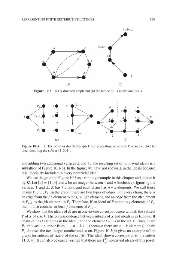
REPRESENTING FINITE DISTRIBUTIVE LATTICES 109
{a,b,c}
{a,b,c,d}
{}
{a}
b
⊥ ⊥
d
ca
(a) (b)
Figure 10.2 (a) A directed graph and (b) the lattice of its nontrivial ideals.
2 3 4
3 4 5
4 5 6
(b)
ek,n−k
e1,n−k
P1
⊥
⊥
⊥
⊥Pk−1
Pk
(a)
Figure 10.3 (a) The poset or directed graph for generating subsets of X of size k. (b) Theideal denoting the subset {1, 3, 4}.
and adding two additional vertices ⊥ and ⊤. The resulting set of nontrivial ideals is asublattice of Figure 10.1(b). In the figure, we have not shown ⊥ in the ideals becauseit is implicitly included in every nontrivial ideal.
We use the graph in Figure 10.3 as a running example in this chapter and denote itby . Let [n] = {1..n} and k be an integer between 1 and n (inclusive). Ignoring thevertices ⊤ and ⊥, has k chains and each chain has n − k elements. We call thesechains P1,… ,Pk. In the graph, there are two types of edges. For every chain, there isan edge from the jth element to the (j + 1)th element, and an edge from the jth elementin Pi+1 to the jth element in Pi. Therefore, if an ideal of P contains j elements of Pi,then it also contains at least j elements of Pi+1.
We show that the ideals of are in one-to-one correspondence with all the subsetsY of X of size k. The correspondence between subsets of X and ideals is as follows. Ifchain Pi has t elements in the ideal, then the element t + i is in the set Y . Thus, chainP1 chooses a number from 1… n − k + 1 (because there are n − k elements); chainP2 chooses the next larger number and so on. Figure 10.3(b) gives an example of thegraph for subsets of size 3 of the set [6]. The ideal shown corresponds to the subset{1, 3, 4}. It can also be easily verified that there are
(nk
)nontrivial ideals of this poset.

110 SLICING
(c)
e1
e2
⊥ ⊥
⊥
⊥ ⊥⊥
e3
e4
e1
e2
e3
e4
e1
e2
e3
e4
(a) (b)
Figure 10.4 Graphs and slices for generating subsets of X when |X| = 4.
As yet another example, consider a poset on n elements such that all pairs of ele-ments are mutually incomparable. The graph when n equals 4 is shown in Figure 10.4.We call this graph n and all of its (nontrivial) ideals are in one-to-one correspon-dence with all subsets of [n].
10.3 PREDICATES ON IDEALS
The slicing technique is crucially based on the notion of predicates on the set ofideals. A predicate is simply a Boolean function from the set of all ideals to {0, 1}.Equivalently, a predicate specifies a subset of the ideals in which the Boolean functionevaluates to 1. In the poset , “does not contain consecutive numbers” is a predicate,which is either true or false for any ideal. For example, it is true for {1, 3, 5} but falsefor {1, 3, 4}. In the Boolean lattice of all subsets of [n], n, “has size k” is a predicatewhich is true if the subset has size k and false otherwise.
We now define various classes of predicates. The class of meet-closed predicates isuseful because they allow us to compute the least ideal that satisfies a given predicate.
Definition 10.2 (meet-closed Predicates) A predicate B is meet-closed for a posetor a graph P if
∀G,H ∈ LI(P) ∶ B(G) ∧ B(H) ⇒ B(G ⊓ H).
The predicate “does not contain consecutive numbers” in the poset ismeet-closed. For example, let G = {1, 3, 7} and H = {2, 4, 6}. Both G and H satisfythe predicate B, “does not contain consecutive numbers.” If we compute the meet ofG and H, we get {1, 3, 6} which also satisfies B. We will show that this is true for allpossible G and H later.
Now consider the predicate “has size k” in the poset n. Let G = {1, 3} and H ={2, 3}. Then, G ⊓ H equals {3} which has different cardinality. Hence, “has size k”is not a meet-closed predicate in n.
It follows from the definition that if there exists any ideal that satisfies ameet-closed predicate B, then there exists the least one obtained by taking themeet of all ideals satisfying B. Note that the predicate false that corresponds to the

PREDICATES ON IDEALS 111
empty subset and the predicate true that corresponds to the entire set of ideals aremeet-closed predicates.
As another example, define a n-size subset of [2n] to satisfy the predicate Catalan ifby putting left parentheses on the specified subset and right parentheses in remainingpositions, one gets a well-balanced string of parentheses. For example, the subset{1, 3, 4} corresponds to the string “()(())” where left parentheses are at positions 1,3, and 4. This subset satisfies Catalan predicate, whereas the subset {1, 4, 5} doesnot. We will use G[i] to denote the ith largest element in the set. To formalize awell-balanced expression, note that if G[i] equals k for any i ∈ [n], then there arei − 1 left parentheses and k − i right parentheses to the left of position k. Therefore,G satisfies the Catalan predicate iff for all i
G[i] − i ≤ i − 1.
Or, equivalentlyG[i] ≤ 2i − 1.
It is now clear that Catalan is a meet-closed (and join-closed) predicate. If G[i] ≤2i − 1 and H[i] ≤ 2i − 1, then min(G[i],H[i]) ≤ 2i − 1.
We now give another characterization of such predicates that will be useful forcomputing the least ideal that satisfies the predicate. To that end, we first define thenotion of a crucial element for an ideal.
Definition 10.3 (Crucial Element) Let P = (E,≤) be a poset. For an ideal G ⫋ Eand a predicate B, we define e ∈ E − G to be crucial for G as:
crucial(G, e,B)def= ∀ ideals H ⊇ G ∶ (e ∈ H) ∨ ¬B(H).
Intuitively, this means that any ideal H, that is at least G, cannot satisfy the predicateunless it contains e.
Definition 10.4 (Linear Predicates) A predicate B is linear iff for all ideals G ⫋ E,
¬B(G) ⇒ ∃e ∈ E − G ∶ crucial(G, e,B).
Now, we have
Theorem 10.5 A predicate B is linear iff it is meet-closed.
Proof: First assume that B is not closed under meet. We show that B is not linear.Since B is not closed under meets, there exist two ideals H and K such that B(H) andB(K) but not B(H ⊓ K). Define G to be H ⊓ K. G is a strict subset of H ⊆ E becauseB(H) but not B(G). Therefore, G cannot be equal to E. We show that B is not linearby showing that there does not exist any crucial element for G. A crucial element e,if it exists, cannot be in H − G because K does not contain e and still B(K) holds.Similarly, it cannot be in K − G because H does not contain e and still B(H) holds.

112 SLICING
It also cannot be in E − (H ∪ K) because H does not contain e and still B(H) holds.We conclude that there does not exist any crucial element for G.
Now assume that B is not linear. This implies that there exists G ⫋ E such that¬B(G) and none of the elements in E − G is crucial. We first claim that E − G cannotbe a singleton. Assume if possible E − G contains only one element e. Then, any idealH that contains G and does not contain e must be equal to G itself. This implies that¬B(H) because we assumed ¬B(G). Therefore, e is crucial contradicting our assump-tion that none of the elements in E − G is crucial. Let W = E − G. For each e ∈ W,we define He as the ideal that contains G, does not contain e, and still satisfies B. SinceW has at least two events, it is easy to see that G is the meet of all He. Therefore, Bis not meet-closed because all He satisfy B but not their meets.
Example 10.6 Consider n shown in Figure 10.4(a). The ideals of this graph cor-respond to subsets of [n] and thus generate the Boolean lattice. Now consider thepredicate B defined to be true on G as “If G contains any odd i < n, then it also con-tains i + 1.” It is easy to verify that B is meet-closed. Given any G for which B doesnot hold, the crucial elements consist of
{i | i e𝑣en, 2 ≤ i ≤ n, i − 1 ∈ G, i ∉ G}.
Example 10.7 Consider the poset . Let the predicate B be “G does not contain anyconsecutive numbers.” Consider any G for which B does not hold. This means thatit has some consecutive numbers. Let i be the smallest number in G such that i − 1is also in G. If i is on chain Pj, then the next element in Pj is crucial. For example,the ideal {1, 3, 4} does not satisfy B. The smallest element whose predecessor is alsoin G is 4 which is on the chain P3. Therefore, the second element in P3 is crucial. Inother words, any ideal that satisfies B and is bigger than {1, 3, 4} is at least {1, 3, 5}.If i is the last element in Pj, then any element in E − G can serve as a crucial elementbecause in this case for any H that contains G, B(H) is false.
Our interest is in detecting whether there exists an ideal that satisfies a givenpredicate B. We assume that given an ideal, G, it is efficient to determine whetherB is true for G. On account of linearity of B, if B is evaluated to be false in someideal G, then we know that there exists a crucial element in E − G. We now make anadditional assumption called the efficient advancement property.
(Efficient Advancement Property) A predicate B satisfies the efficient advancementproperty if there exists an efficient (polynomial time) function to determine a crucialelement whenever B evaluates to false on any cut.
We now have

PREDICATES ON IDEALS 113
(1) boolean function detect(B:boolean_predicate, P:graph)(2) var(3) G: ideal initially G = {⊥};(4)(5) while (¬B(G) ∧ (G ≠ P)) do(6) Let e be such that crucial(e,G,B) in P;(7) G ∶= G ∪ {e}.(8) endwhile;(9) if B(G) return true;(10) else return false;
Figure 10.5 An efficient algorithm to detect a linear predicate.
Theorem 10.8 If B is a linear predicate with the efficient advancement property, thenthere exists an efficient algorithm to determine the least ideal that satisfies B (if any).
Proof: An efficient algorithm to find the least cut in which B is true is given inFigure 10.5. We search for the least ideal starting from the ideal {⊥}. If the predicateis false in the ideal, then we find a crucial element using the efficient advancementproperty and then repeat the procedure.
Assuming that crucial(e,G,B) can be evaluated efficiently for a given graph, wecan determine the least ideal that satisfies B efficiently even though the number ofideals may be exponentially larger than the size of the graph. As an example, to findthe least ideal in that satisfies “does not contain consecutive numbers,” we startwith the ideal {1, 2, 3}. Since 1 and 2 are consecutive, we advance along P2 to theideal {1, 3, 4}, which still does not satisfy the predicate. We now advance along P3to the ideal {1, 3, 5} which is the smallest ideal that satisfies the given predicate.
So far, we have focused on meet-closed predicates. All the definitions and ideascarry over to join-closed predicates. If the predicate B is join-closed, then one cansearch for the largest ideal that satisfies B in a fashion analogous to finding the leastideal when it is meet-closed.
Predicates that are both meet-closed and join-closed are called regular predicates.
Definition 10.9 (Regular Predicates) A predicate is regular if the set of ideals thatsatisfy the predicate forms a sublattice of the lattice of ideals.
Equivalently, a predicate B is regular with respect to P if it is closed under ⊔ and ⊓,i.e.,
∀G,H ∈ LI(P) ∶ B(G) ∧ B(H) ⇒ B(G ⊔ H) ∧ B(G ⊓ H)
The set of ideals that satisfy a regular predicate forms a sublattice of the latticeof all ideals. Since a sublattice of a distributive lattice is also distributive, the set of

114 SLICING
ideals that satisfy a regular predicate forms a distributive lattice. From Birkhoff’stheorem, we know that a distributive lattice can be equivalently represented using theposet of its join-irreducible elements. The poset of join-irreducible elements providesa compact way of enumerating all ideals that satisfy the predicate and will be usefulin efficient solving of combinatorial problems.
There are two important problems with this approach of finding the set of idealsthat satisfy a given predicate. First, what if the predicate is not regular? Is it stillpossible to represent the set of ideals satisfying B compactly? Second, we need tocalculate the structure that captures the set of ideals satisfying B efficiently. Theseproblems are addressed in the following section.
The notion of a slice will be used to represent the subset of ideals that satisfy B in aconcise manner. The slice of a directed graph P with respect to a predicate B (denotedby slice(P,B)) is a graph derived from P such that all the ideals in LI(P) that satisfy Bare included in LI(slice(P,B)). Note that the slice may include some additional idealsthat do not satisfy the predicate. Formally,
Definition 10.10 (Slice) A slice of a graph P with respect to a predicate B is thedirected graph obtained from P by adding edges such that:
(1) it contains all the ideals of P that satisfy B and(2) of all the graphs that satisfy (1), it has the least number of ideals.
We first show that given a distributive lattice L generated by the graph (poset) P,every sublattice of L can be generated by a graph obtained by adding edges to P.
Theorem 10.11 Let L be a finite distributive lattice generated by the graph P. Let L′
be any sublattice of L. Then, there exists a graph P′ that can be obtained by addingedges to P that generates L′.
Proof: Our proof is constructive. We show an algorithm to compute P′. For everyvertex e ∈ P, let I(e) be the set of ideals of P containing e. Since L is the set ofall ideals of P, we can view I(e) as a subset of L. In rest of the proof, we will notdistinguish between an ideal of the graph P and the corresponding element in latticeL. Let I(e,L′) be the subset of I(e) that is contained in L′, i.e., I(e,L′) = I(e) ∩ L′.On the basis of the set I(e,L′), we define J(e,L′) as follows. If I(e,L′) is empty, thenJ(e,L′) is defined to be the trivial ideal of P that includes the ⊤ element. Otherwise,J(e,L′) is defined as the least element of I(e,L′). Since L′ is a sublattice, it is clear thatif the set of ideals that include e are in L′, then their intersection (meet) also includese and is in L′. Thus, J(e,L′) is well defined.
Note that J(⊥, L′) corresponds to the least element of L′ and J(⊤, L′) correspondsto the trivial ideal that includes ⊤.
Now, we add the following edges to the graph P. For every pair of vertices e, f suchthat J(e,L′) ≤ J(f ,L′), we add an edge from e to f . We now claim that the resultinggraph P′ generates L′.
Pick any nontrivial ideal G of P′, i.e., an ideal that includes ⊥ and does not include⊤. We show that G = ∪e∈GJ(e,L′). This will be sufficient to show that G ∈ L′ becauseG is a union of ideals in L′ and L′ is a lattice. Since e ∈ J(e,L′), it is clear that G ⊆

PREDICATES ON IDEALS 115
∪e∈GJ(e,L′). We show that G ⊇ ∪e∈GJ(e,L′). Let f ∈ J(e,L′) for some e. This impliesthat J(f ,L′) ⊆ J(e,L′) because J(f ,L′) is the least ideal containing f in L′. By ouralgorithm, there is an edge from f to e in P′, and since G is an ideal of P′ that includese, it also includes f . Thus G ⊇ ∪e∈GJ(e,L′).
Conversely, pick any element G of L′. We show that G is a nontrivial ideal of P′.Since L′ ⊆ L and L correspond to nontrivial ideals of P, it is clear that G is a nontrivialideal of P. Our obligation is to show that it is a nontrivial ideal of P′ as well. Assume,if possible, G is not a nontrivial ideal of P′. This implies that there exists vertices e, fin P′ such that f ∈ G, e ∉ G and (e, f ) is an edge in P′. The presence of this edge in P′,but not in P implies that J(e,L′) ⊆ J(f ,L′). Since f ∈ G and G ∈ L′, from definitionof J(f ,L′), we get that J(f ,L′) ⊆ G. However, this implies J(e,L′) ⊆ G, i.e., e ∈ G, acontradiction.
Now, the following result is easy.
Theorem 10.12 For any P and B, slice(P,B) exists and is unique.
Proof: First note that intersection of sublattices is also a sublattice. Now given anypredicate B consider all the sublattices that contain all the ideals that satisfy B. Theintersection of all these sublattices gives us the smallest sublattice that contains allthe ideals. From Theorem 10.11, we get that there exists a graph that generates thissublattice.
The procedure outlined in the above-mentioned proof is not efficient because itrequires us to take intersection of all bigger sublattices. We now show how to effi-ciently compute slices for the predicates for which there exists an efficient detectionalgorithm. The slicing algorithm is shown in Figure 10.6. It takes as input a graphP and a Boolean predicate B. The algorithm constructs the slice by adding edges tothe graph P. For this purpose, it initializes in line (3) a graph R as P. In rest of thefunction, edges are added to R, which is finally returned.
The addition of edges is done as follows. For every pair of vertices, e and f , in thegraph P, the algorithm constructs Q from P by adding edges from f to ⊥ and ⊤ toe. Owing to these edges in Q, all nontrivial ideals of Q contain f and do not containe. We now invoke the detection algorithm on Q. If the detection algorithm returnsfalse, then we know that there is no nontrivial ideal of P that contains f but does notcontain e. Therefore, all ideals that satisfy B have the property that if they include f ,they also include e. Hence, we add an edge from e to f in the graph R. We continuethis procedure for all pairs of vertices. Theorem 10.13 shows the correctness of thisprocedure.
Theorem 10.13 Let P be a directed graph. Let R be the directed graph output by thealgorithm in Figure 10.6 for a predicate B. Then R is the slice of P with respect to B.

116 SLICING
(1) graph function computeSlice(B:boolean_predicate, P: graph)(2) var(3) R: graph initialized to P;(4) begin(5) for every pair of nodes e, f in P do(6) Q := P with the additional edges (f , ⊥) and (⊤, e);(7) if detect(B,Q) is false(8) add edge (e, f ) to R;(9) endfor(10) return R;(11) end;
Figure 10.6 An efficient algorithm to compute the slice for a predicate B.
Proof: Let LI(P,B) denote the set of ideals of P that satisfy B. We first show thatLI(R) ⊇ LI(P,B). Adding an edge (e, f ) in R eliminates only those ideals of P thatcontain f but do not contain e. However, all those ideals do not satisfy B becausethe edge (e, f ) is added only when detect(B,Q) is false. Thus, all the ideals of P thatsatisfy B are also the ideals of R.
Next, we show that the LI(R) is the smallest sublattice of LI(P) that includesLI(P,B). Let M be a graph such that LI(M) ⊇ LI(P,B). Assume that if possible LI(M)is strictly smaller than LI(R). This implies that there exists two vertices e and f suchthat there is an edge from e to f in M but not in R. Since R is output by the algorithm,detect(B,Q) is true in line (7); otherwise, an edge would have been added from e tof . But, this means that there exists an ideal in P, which includes f , does not include e,and satisfies B. This ideal cannot be in LI(M) due to the edge from e to f contradictingour assumption that LI(P,B) ⊆ LI(M).
Theorem 10.13 allows us to compute the slice for any predicate that can bedetected efficiently. For example, relational predicates can be detected efficientlyusing max-flow techniques [CG95].
When the predicate is known to be linear, we can use a more efficient and directalgorithm to compute the slice as shown in Figure 10.7. The algorithm determines forevery element e ∈ P, the least order ideal of P that includes e and satisfies B. Since Bis a linear predicate and the condition "includes e" is also linear, it follows that leastis well-defined whenever there are satisfying cuts. The correctness of this algorithmis left as an exercise.
10.4 APPLICATION: SLICING DISTRIBUTED COMPUTATIONS
Since the set of all consistent global states form a distributive lattice, we can use theslicing method to represent a subset of interesting global states. For regular predicates,
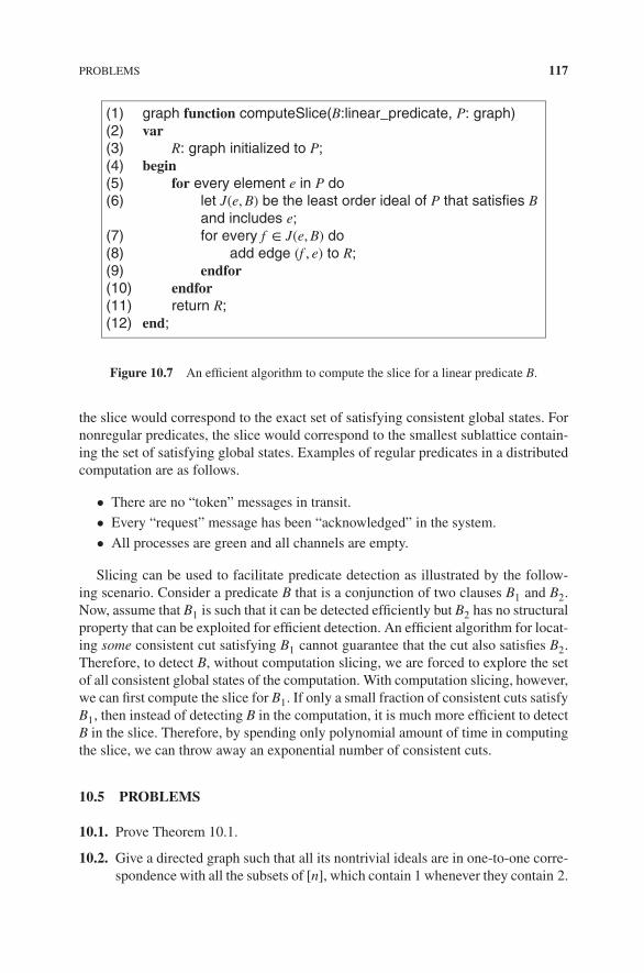
PROBLEMS 117
(1) graph function computeSlice(B:linear_predicate, P: graph)(2) var(3) R: graph initialized to P;(4) begin(5) for every element e in P do(6) let J(e,B) be the least order ideal of P that satisfies B
and includes e;(7) for every f ∈ J(e,B) do(8) add edge (f , e) to R;(9) endfor(10) endfor(11) return R;(12) end;
Figure 10.7 An efficient algorithm to compute the slice for a linear predicate B.
the slice would correspond to the exact set of satisfying consistent global states. Fornonregular predicates, the slice would correspond to the smallest sublattice contain-ing the set of satisfying global states. Examples of regular predicates in a distributedcomputation are as follows.
• There are no “token” messages in transit.
• Every “request” message has been “acknowledged” in the system.
• All processes are green and all channels are empty.
Slicing can be used to facilitate predicate detection as illustrated by the follow-ing scenario. Consider a predicate B that is a conjunction of two clauses B1 and B2.Now, assume that B1 is such that it can be detected efficiently but B2 has no structuralproperty that can be exploited for efficient detection. An efficient algorithm for locat-ing some consistent cut satisfying B1 cannot guarantee that the cut also satisfies B2.Therefore, to detect B, without computation slicing, we are forced to explore the setof all consistent global states of the computation. With computation slicing, however,we can first compute the slice for B1. If only a small fraction of consistent cuts satisfyB1, then instead of detecting B in the computation, it is much more efficient to detectB in the slice. Therefore, by spending only polynomial amount of time in computingthe slice, we can throw away an exponential number of consistent cuts.
10.5 PROBLEMS
10.1. Prove Theorem 10.1.
10.2. Give a directed graph such that all its nontrivial ideals are in one-to-one corre-spondence with all the subsets of [n], which contain 1 whenever they contain 2.

118 SLICING
10.3. Compute the slice of the graph in the previous question for subsets, whichalways contain n − 1.
10.4. Show that whenever B is linear, the order ideal JB(e) defined as the least orderideal that satisfies B and includes e is a join-irreducible element of the slice oforder ideals that satisfy B. Conversely, every join-irreducible elements of theslice is of the form JB(e) for some e.
10.5. Show the correctness of the algorithm in Figure 10.7.
10.6. Given slices for predicates B1 and B2 with respect to a computation P, givealgorithms to compute slices for B1 ∧ B2, B1 ∨ B2, and ¬B1.
10.7. Often, we are interested in temporal properties relating to the sequence of statesduring an execution rather than just the initial and final states. For example, theliveness property in the dining philosophers problem, “a philosopher, when-ever gets hungry, eventually gets to eat,” is a temporal property. We say thata consistent cut C satisfies EF(B) if B holds for some consistent cut on somepath from C to the final consistent cut. We say that a consistent cut C satisfiesEG(B) (respectively AG(B)) if B holds for all cuts on some (respectively all)path from C to the final consistent cut. Given a distributed computation, and aslice for a regular predicate B, give algorithms to compute slice for EF(B) andAG(B).
10.6 BIBLIOGRAPHIC REMARKS
The definition of slicing is from Garg and Mittal [GM01], Mittal and Garg [MG01b].The algorithm in Figure 10.6 is from Mittal, Sen, and Garg [MSG07].

11APPLICATIONS OF SLICING TOCOMBINATORICS
11.1 INTRODUCTION
A combinatorial problem usually requires enumerating, counting, or ascertainingexistence of structures that satisfy a given property B in a set of structures L. We nowshow that slicing can be used for solving such problems mechanically and efficiently.Specifically, we give an efficient (polynomial time) algorithm to enumerate, count,or detect structures that satisfy B when the total set of structures is large but the setof structures satisfying B is small. We illustrate the slicing method by analyzingproblems in integer partitions, set families, and the set of permutations.
Consider the following combinatorial problems:
(Q1) Count the number of subsets of the set [n] (the set {1… n}), which have sizem and do not contain any consecutive numbers.
(Q2) Enumerate all integer partitions less than or equal to the partition(𝜆1, 𝜆2,… , 𝜆n) in which 𝜆1 equals 𝜆2.
(Q3) Give the number of permutations of [n] in which i less than or equal to jimplies that the number of inversions of i is less than or equal to the numberof inversions of j.
Our goal in this chapter is to show how such problems can be solved mechanicallyand efficiently for any fixed values of the parameters n and m.
Introduction to Lattice Theory with Computer Science Applications, First Edition. Vijay K. Garg.© 2015 John Wiley & Sons, Inc. Published 2015 by John Wiley & Sons, Inc.

120 APPLICATIONS OF SLICING TO COMBINATORICS
It is important to note that someone trained in combinatorics may be able to solveall of these problems efficiently (and the reader is encouraged to solve these problemsbefore reading further). Our emphasis is on techniques that can be applied mechani-cally. On the other hand, note that for the fixed values of n and m, all the sets aboveare finite and therefore all the problems can be solved mechanically. Our emphasis ison efficiency. To be more precise, let L be a large set of combinatorial structures (forexample, all subsets of {1… n} of size m and all permutations of [n]) Each combina-torial problem requires enumerating, counting, or searching the subset of structuresthat satisfy a given property B. Call this set LB ⊆ L. For example, in the problem (Q1),L is the set of all subsets of [n] of size m and LB is the set of all subsets of [n] of sizem that do not contain any consecutive numbers. For any fixed set of parameters m andn, the size of L is large but finite, enabling one to enumerate all possible structuresand then to check each one of them for the property B. This approach results in analgorithm that requires time proportional to the size of the set L which is exponentialin n (or m). We show a technique that provides answers to some combinatorial prob-lems in polynomial time and for others, such as those involving enumeration, in timeproportional to the size of LB (and not L).
To explain the slicing technique, we use the term small to mean polynomial in nand m, and large to mean exponential in n or m. Thus, the set L is large. We firstbuild a small structure P such that all elements of L can be generated by P. Second,we compute a slice of P with respect to B, denoted by PB, such that PB generatesall elements of LB. PB is a small structure and can be efficiently analyzed to answerquestions about LB or enumerate all elements of LB.
11.2 COUNTING IDEALS
For counting the number of elements in L and its sublattices, we use N(P) to denotethe number of ideals of the poset P. Since our interest is in efficient calculation ofN(P), we will restrict the dimension of the partial order generating the lattice. Deter-mining whether a poset P with n points is 2-dimensional and isomorphism testingfor 2-dimensional orders can be done in O(n2) time [Spi85]. All the posets used inthis chapter are two dimensional. The following lemma shows that the number ofideals of a poset can be calculated efficiently for series–parallel posets (a specialcase of two-dimensional posets) [FLST86]. For generalization to counting ideals oftwo-dimensional posets, see Steiner [Ste84] and Chapter 13.
Lemma 11.1 (Counting Lemma)
1. If Q is an extension of P then N(Q) ≤ N(P).2. (Parallel) Let P + Q be the disjoint union (or direct sum) of posets P and Q.
Then, N(P + Q) = N(P)N(Q).3. Let P ⊕ Q be the ordinal sum of posets P and Q. Then, N(P ⊕ Q) = N(P) +
N(Q) − 1.

BOOLEAN ALGEBRA AND SET FAMILIES 121
4. Assume that P can be decomposed into the least number of chains C1,C2,…Cn.Then
N(P) ≤n∏
i=1
(|Ci| + 1).
When each chain is at most m in length, we get that N(P) ≤ (m + 1)n.
11.3 BOOLEAN ALGEBRA AND SET FAMILIES
Let X be a ground set on n elements. Assume that we are interested in the sets ofsubsets of X. By using ⊆ as the order relation, we can view it as a distributive latticeL. This lattice has n + 1 levels and each level set of rank k in the Boolean latticecorresponds to
(nk
)sets of size k. L is generated by the directed graph in Figure 11.1(a).
It is easy to verify that there is a bijection between nontrivial ideals of the graph andsubsets of X.
Now consider all subsets of X such that if they include ei then they also includeej. To obtain the slice with respect to this predicate, we just need to add an edge fromej to ei. Figure 11.1(b) shows the slice with respect to the predicate “if e3 is includedthen so is e2.” To ensure the condition that ei is always included, we simply add anedge from ei to ⊥ and to ensure that ei is never included in any subset, we add an edgefrom ⊤ to ei. Figure 11.1(c) shows the slice that gives all subsets that always containe1, never contain e4, and contain e2 whenever they contain e3.
As an application, we now solve some combinatorial problems. Let n be even. Weare required to calculate the total number of subsets of [n] which satisfy the propertythat if they contain any odd integer i, then they also contain i + 1 (or equivalently,compute the number of ways to select groups from n∕2 couples such that a wifeis always accompanied by her husband in the group although a husband may notbe accompanied by his wife). Although this problem can be solved directly by acombinatorial argument, we will show how the slicing method can be applied. Wefirst construct the poset that generates all the subsets of [n]. It is Figure 11.1(a) in thecase of 4. We now define the subset of interest by a predicate B. For any subset G of[n], we let B(G) to be true if G contains i + 1 whenever it contains any odd integer i.From our discussion of regular predicates, it is clear that B is regular. To compute theslice, it is sufficient to have a predicate detection algorithm. Detecting the least idealthat satisfies B can be done efficiently because it satisfies the efficient advancementproperty: “If an ideal does not satisfy B, then there is some unaccompanied wifeand therefore the element corresponding to the husband is crucial.” By applying thepredicate detection algorithm repeatedly, we can determine all the edges that need tobe added to get the slice. In this example, it is sufficient to add an edge from ei+1 toei for odd i. The slice consists of n∕2 chains each with exactly 2 elements (ignoring⊥ and ⊤). From the counting lemma (Lemma 11.1), it follows that the total numberof ideals is (2 + 1)n∕2 = 3n∕2. The reader should note that for any fixed value of n, theproblem can be solved by a computer automatically and efficiently (because the sliceresults in a series-parallel poset).

122 APPLICATIONS OF SLICING TO COMBINATORICS
(c)
e1
e2
⊥ ⊥
⊥
⊥ ⊥⊥
e3
e4
e1
e2
e3
e4
e1
e2
e3
e4
(a) (b)
Figure 11.1 Graphs and slices for generating subsets of X when |X| = 4.
As another example, let us enumerate the subsets {a1,… , am} of n such that forall i and j, ai does not divide aj.
We have the following result.
Lemma 11.2 Consider the graph Q obtained from Figure 11.1(a) by adding an edgefrom i to j whenever i divides j. Then, Q can be used to enumerate all subsets of [n]which do not contain any ai and aj such that ai divides aj.
Proof: Define B(G) as ∀i, j ∶ (i ≠ j) ∧ (ai di𝑣ides aj) ∧ (aj ∈ G) ⇒ (ai ∈ G).It is clear that B is a regular predicate and the resulting slice is acyclic. Each desired
subset is simply the antichains of the poset so obtained. There is 1-1 correspondencebetween antichains and ideals.
11.4 SET FAMILIES OF SIZE K
It is important to note that regularity of B is dependent on the lattice structure of L.For example, in many applications of set families, we are interested in sets of a fixedsize k. The predicate B that the ideal is of size k is not regular. However, by consid-ering alternative posets, this set family can still be analyzed. Here, the appropriateposet to use is the graph (k, n − k) shown in Figure 10.3. As shown in Chapter 10,the set of ideals of (k, n − k) are in 1-1 correspondence with all the subsets of [n]of size k.
Note that by considering all possible choices made by Pk, this method gives aneasy proof of the combinatorial identity
(nk
)
=n−1∑
m=k−1
(m
k − 1
)
.
Let us now apply the slicing method to the first combinatorial problem (Q1) men-tioned in the introduction. Assume that we are interested in counting all subsets ofn of size k, which do not have any consecutive numbers. For (Q1), our interest is in

INTEGER PARTITIONS 123
Pk
⊥
⊥
Pk−1
P1
ek,n−k
e1,n−k
Figure 11.2 Slice for the predicate “does not contain consecutive numbers”.
ideals that correspond to subsets without any consecutive numbers. It can be verifiedthat an ideal G satisfies B if whenever Pi has t elements in G, Pi+1 has at least t + 1elements in G. This condition is linear and we can use the algorithm in Figure 10.6to compute the slice. Figure 11.2 shows the slice that includes precisely those sub-sets that do not contain consecutive numbers. By collapsing all strongly connectedcomponents and by removing the transitively implied edges, we get a graph that is iso-morphic to (k, n − k − (k − 1)) (i.e., the original graph when there are k chains andeach chain has only n − k − (k − 1) elements). Therefore, the total number of orderideals is
(n−k+1k
). Again one can come up with a combinatorial argument to solve the
problem (for example, see Theorem 13.1 and Example 13.1 in van Lint [vLW92]),but it is easier to solve the problem using slicing.
All the above-mentioned constructions can be generalized to multidimensionalgrids to obtain results on multinomials instead of binomials.
11.5 INTEGER PARTITIONS
In this section, we apply slicing to integer partitions that have been studied by math-ematicians for a long time.
Definition 11.3 𝜆 = (𝜆1, ..., 𝜆k) is an unordered partition of the integer n if
1. ∀i ∈ [1, k − 1] ∶ 𝜆i ≥ 𝜆i+1
2.∑k
i=1 𝜆i = n
Definition 11.4 p(n) is the number of unordered partitions of the integer n.
Definition 11.5 A Ferrer’s diagram for an integer partition 𝜆 = (𝜆1, ..., 𝜆k) of integern is a matrix of dots where the ith row contains 𝜆i dots (example Figure 11.3). Thus,each row represents the size of a partition and the number of rows represents thenumber of parts in the partition.

124 APPLICATIONS OF SLICING TO COMBINATORICS
7 = 4 + 2 + 1
Figure 11.3 Ferrer’s diagram for the integer partition (4, 2, 1) for 7.
Figure 11.4 An Application of Ferrer’s diagram.
As an application of Ferrer’s diagram, we show that the number of partitions ofn with k parts and the largest part equal to m is equal to the number of partitions ofn with m parts and the largest part equal to k. The two numbers can be shown to beequal by noting that there exists a one-to-one correspondence between a partition 𝜆
of n with k parts such that the largest part is equal to m and a partition 𝜆′ of n with mparts such that the largest part is equal to k. This is because 𝜆 can be transformed toa partition of the latter type by rotating its Ferrer’s diagram as shown in Figure 11.4.
We now define an order on the set of partitions. Given two partitions𝜆 = (𝜆1, 𝜆2,… , 𝜆m), 𝛿 = (𝛿1, 𝛿2,… , 𝛿n), we define
𝜆 ≥ 𝛿 ≡ (m ≥ n) ∧ (∀i ∶ 1 ≤ i ≤ n ∶ 𝜆i ≥ 𝛿i).
This can also be viewed in terms of containment in the Ferrer’s diagram i.e. 𝜆 ≥ 𝛿
if the Ferrer’s diagram for 𝛿 is contained in the Ferrer’s diagram of 𝜆. For example,(4, 3, 2) ≥ (2, 2, 2) as shown in figure 1.7.
Definition 11.6 (Young’s Lattice) Given a partition 𝜆, Young’s lattice Y𝜆 is the lat-tice of all partitions that are less than or equal to 𝜆.
The Young’s lattice for (3, 3, 3) first introduced in Chapter 1 is shown in figure 11.5.We claim that Y𝜆 is the set of ideals of the poset corresponding to the Ferrer’s dia-
gram of 𝜆 (an example of the poset for partition (3, 3, 3) is shown in Figure 11.6). Thisclaim holds because for any ideal 𝛿 of the Ferrer’s diagram, the components satisfy∀i ≥ j ∶ 𝛿i ≥ 𝛿j. Since Young’s lattice is a lattice of ideals, it is clearly distributive.One can see that the lattice of subsets of size k from the set of size n is a special case

INTEGER PARTITIONS 125
(3,1,1)
(3)
(3,3,1)
(3,3,3)
(3,3)
(1)
(2,1)
(3,2,1)
(3,3,2)
(3,2,2)
(2,2,2)
(1,1,1)
(1,1) (2)
(0)
(3,1)(2,1,1)
(2,2,1) (3,2)
(2,2)
Figure 11.5 Young’s lattice for (3, 3, 3).
3
01 2 3
0 1 2 3
01 2
Figure 11.6 The poset corresponding to Ferrer’s diagram of (3, 3, 3).
of Young’s lattice when all 𝜆i’s are equal. Therefore, the number of integer partitionswhose Ferrer’s diagrams fit in a box of size k by n − k is equal to
(nk
)(providing an
alternate proof of Theorem 3.2 in Stanton and White [SW86]). Let q(l, k,m) denotethe number of partitions of l whose Ferrer’s diagram fit in a box of size k by m. Sincep(n) has at most n parts and each part is at most n, it follows that the nth level ofY(n,n,…,n)⏟⏞⏟⏞⏟
n
contains all partitions of n. In Chapter 14, we use enumeration of the level
set of the ideal lattice to enumerate all partitions of n. An example of level sets canbe seen in Figure 11.5. The third level has three partitions: 3, (2,1), and (1,1,1). Thisset corresponds to p(3).

126 APPLICATIONS OF SLICING TO COMBINATORICS
(a) (b)
0
0
0
1 2 3
41 2
1 2
3
3
2
3
4
12
0
2
Figure 11.7 Slice for 𝛿2 = 2.
By summing up the sizes of all level sets, it follows that
(nk
)
=k(n−k)∑
l=0
q(l, k, n − k).
Since the poset that generates the corresponding Young’s lattice is symmetric withrespect to k and m, we get that q(l, k,m) equals q(l,m, k); and since the poset is dualof itself (i.e., we get back the same poset when all arcs are reversed), we also get thatq(l, k,m) equals q(mk − l, k,m). All these results are generally derived using Gaussianpolynomials (see van Lint [vLW92]).
We now examine the partitions which have some additional conditions imposed onthem. These additional conditions can then be viewed as predicates and the slicingmethod could be used to give us a graph which could generate all such partitions.Some very natural and interesting partitions are as follows:All partitions that are less than or equal to 𝜆
• with odd parts• with distinct parts• with even parts• with (𝜆1 = 𝜆2)• with (𝜆k = 1)
Interestingly, it turns out that all these predicates are regular! The reader is encouragedto prove that this is indeed true.
Assume that we are interested in all partitions less than or equal to (4, 3, 3) such thattheir second component is some fixed value, say b. It is easy to verify that partitions𝛿 ∈ Y𝜆 such that 𝛿2 = b form a sublattice, and therefore, the condition 𝛿2 = b is aregular predicate.
Figure 11.7(a) shows the slice of partitions in which 𝛿2 = 2. Since the second partmust be 2, additional edges ensure that the ideal of the graph has exactly two elementsfrom P2. On collapsing the strongly connected components and transitively reduc-ing the graph, we get the series–parallel graph Figure 11.7(b). By applying countinglemma, we get that there are (2 + 1)(2 + 1) = 9 such partitions that can all be enu-merated automatically using Figure 11.7(b). They are as follows:
{220, 221, 222, 320, 321, 322, 420, 421, 422}

PERMUTATIONS 127
(a) (b)
Figure 11.8 Slice for “distinct parts.”
As another example assume that we are interested in all partitions less than 𝜆 =(4, 3, 3), which have distinct parts. Figure 11.8(a) gives the slice and Figure 11.8(b)gives the graph after simplification. The graph is equivalent to that of subsets of size 3from [5]. Hence, there are
(53
)such partitions. These partitions can also be enumerated
from the figure. They are as follows:
{210, 310, 410, 320, 420, 430, 321, 421, 431, 432}.
Some other subsets of partitions discussed in the literature are “partitions with oddnumber of parts,” “partitions with distinct odd parts,” “partitions with even numberof parts,” “kth part is at most h,” etc. These are all regular predicates.
Now the reader may also see the solution for the second problem (Q2) mentionedin the introduction—enumerating all partitions in the Young’s lattice Y𝜆 with the firstpart equal to the second part. We simply define the predicate B on a partition 𝛿 to betrue when 𝛿1 equals 𝛿2. It is clear that the predicate is closed under joins and meetsand is therefore a regular predicate. One can draw the slice and conclude that thenumber of partitions 𝛿 in Y𝜆 satisfying 𝛿1 = 𝛿2 is equal to the number of partitionsin Y𝛿 where 𝛿 = (𝜆2, 𝜆3,… , 𝜆k). The slice can also be used to enumerate all requiredpartitions.
11.6 PERMUTATIONS
We first show a poset such that its ideals can be mapped to all permutations of nsymbols. Figure 11.9 shows the poset T(n) that generates all permutations for n = 5.The poset T(n) consists of n − 1 disjoint chains, P1, ..,Pn−1 where Pi has i elements.There are multiple ways to interpret a given ideal G. We use G[i] to denote the numberof elements from chain Pi included in the ideal G.
1. The simplest way is to view the permutation as a problem of putting n symbolsinto n places. G[i] indicates the place for the symbol i + 1. We start with placingn and then go backward to 1. The symbol n has n choices for places. This wecan determine from G[n − 1], which is a number in {0..n − 1}. Given the placefor symbol n, the symbol n − 1 has n − 1 choices of places, which is given byG[n − 2] because one place is already occupied. This process is repeated tillsymbol 2 is placed. Finally, symbol 1 has no choice.
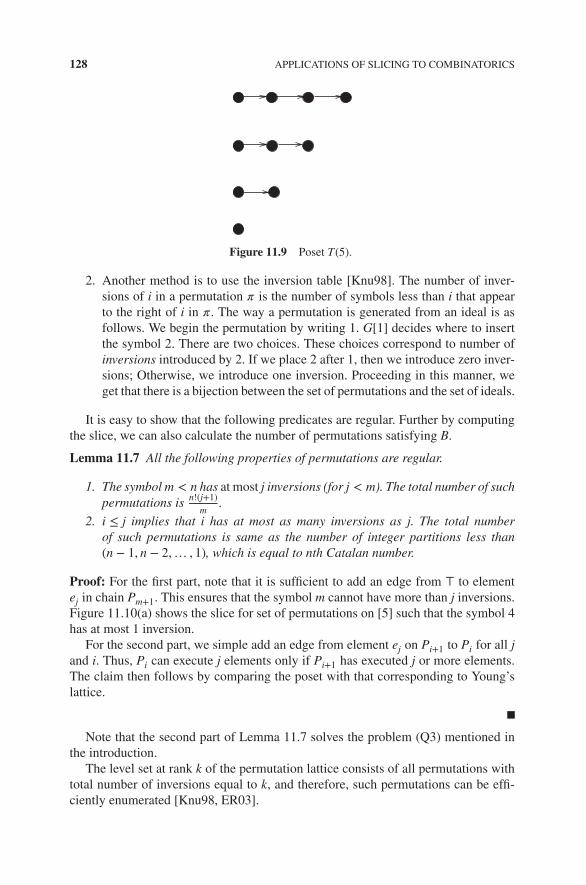
128 APPLICATIONS OF SLICING TO COMBINATORICS
Figure 11.9 Poset T(5).
2. Another method is to use the inversion table [Knu98]. The number of inver-sions of i in a permutation 𝜋 is the number of symbols less than i that appearto the right of i in 𝜋. The way a permutation is generated from an ideal is asfollows. We begin the permutation by writing 1. G[1] decides where to insertthe symbol 2. There are two choices. These choices correspond to number ofinversions introduced by 2. If we place 2 after 1, then we introduce zero inver-sions; Otherwise, we introduce one inversion. Proceeding in this manner, weget that there is a bijection between the set of permutations and the set of ideals.
It is easy to show that the following predicates are regular. Further by computingthe slice, we can also calculate the number of permutations satisfying B.
Lemma 11.7 All the following properties of permutations are regular.
1. The symbol m < n has at most j inversions (for j < m). The total number of suchpermutations is n!(j+1)
m.
2. i ≤ j implies that i has at most as many inversions as j. The total numberof such permutations is same as the number of integer partitions less than(n − 1, n − 2,… , 1), which is equal to nth Catalan number.
Proof: For the first part, note that it is sufficient to add an edge from ⊤ to elementej in chain Pm+1. This ensures that the symbol m cannot have more than j inversions.Figure 11.10(a) shows the slice for set of permutations on [5] such that the symbol 4has at most 1 inversion.
For the second part, we simple add an edge from element ej on Pi+1 to Pi for all jand i. Thus, Pi can execute j elements only if Pi+1 has executed j or more elements.The claim then follows by comparing the poset with that corresponding to Young’slattice.
Note that the second part of Lemma 11.7 solves the problem (Q3) mentioned inthe introduction.
The level set at rank k of the permutation lattice consists of all permutations withtotal number of inversions equal to k, and therefore, such permutations can be effi-ciently enumerated [Knu98, ER03].

BIBLIOGRAPHIC REMARKS 129
(b) (a)
Figure 11.10 Slice for subsets of permutations.
11.7 PROBLEMS
11.1. Give an algorithm to enumerate the subsets {a1,… , am} of n such that for all iand j, ai does not divide aj.
11.2. Compute the slice for a Catalan predicate that contains all n size subsets of 2nthat are Catalan.
11.3. Consider the set of all n-tuples such that ith coordinate belongs to [mi]. This sethas m1m2 …mn elements and is the ideal lattice of disjoint union of n chains,C1,C2,… ,Cn such that |Ci| = mi − 1. This set reduces to the Boolean latticewhen all mi equal 2 and to the set of all permutations when mi = i. Show thateach of the following predicates is regular, and therefore, the subsets corre-sponding to them can be enumerated efficiently.
(a) The set of all tuples (a1, a2,… , an) such that ∀i, j ∶ i ≤ j ⇒ ai ≤ aj.
(b) The set of all tuples (a1, a2,… , an) such that ai ≥ c (or ai = c, ai ≠ c etc.)for some constant c.
(c) The set of all tuples (a1, a2,… , an) such that ai = aj for fixed i and j.
11.4. Consider the set of independent sets in a bipartite graph (X,Y ,E). Every inde-pendent set S can be written as union of SX = S ∩ X and SY = S ∩ Y . Given twoindependent sets S and T , define
S ≤ T ≡ SX ⊆ TX ∧ SY ⊇ TY .
(a) Show that the set of all independent sets forms a distributive lattice.(b) Show that the set of independent sets that contain x only if they contain yforms a sublattice and that its slice can be computed for enumeration.
11.8 BIBLIOGRAPHIC REMARKS
The discussion on applications of slicing to combinatorics is taken from Garg[Gar06].

12INTERVAL ORDERS
12.1 INTRODUCTION
This chapter covers weak orders (ranking), semiorders, and interval orders. All ofthese partial orders are “close” to a total order. The relationship between these ordersis as follows. Every weak order is also a semiorder, and every semiorder is also aninterval order.
12.2 WEAK ORDER
A weak order, also called ranking, is a slight generalization of a total order.
Definition 12.1 (Weak Order) A poset (X,≤) is a weak order or a ranking if thereexists a function f ∶ X → ℕ such that ∀x, y ∈ X ∶ x < y ≡ f (x) < f (y).
The term “weak order” is somewhat of a misnomer because a weak order has alot of order. To allow for easy visualization of such orders, we will use the term“ranking” instead of the more accepted term “weak order.” The set of elements in aranking which have the same f value is called a rank. For example, the poset (X,≤)shown in Figure 12.1 is a ranking because we can assign f (a) = 0, f (b) = f (c) = 1,and f (d) = 2. Here, b and c are in the same rank. The difference between a chain anda ranking is that a chain requires existence of a one-to-one mapping such that x < y ifff (x) < f (y). For a ranking, we drop the requirement of the function to be one-to-one.
A chain is a ranking in which every rank is of size 1. An antichain is also a rankingwith exactly one rank.
Introduction to Lattice Theory with Computer Science Applications, First Edition. Vijay K. Garg.© 2015 John Wiley & Sons, Inc. Published 2015 by John Wiley & Sons, Inc.

132 INTERVAL ORDERS
d
a
b c
Figure 12.1 A poset that is a ranking.
All incomparable
Figure 12.2 Examples of weak orders (or rankings.)
Rankings occur naturally in many applications. Any single scale of measurementprovides us a ranking function. For example, in an election, if we order all candidatesbased on the number of votes they receive, the resulting order is a ranking. In acomputer system, jobs are typically assigned a priority level (say a number between1 and n) (Figure 12.2). This assignment imposes a ranking on all jobs.
An alternative characterization of rankings is as follows.
Theorem 12.2 P is a ranking iff it does not have 1 + 2 as a subposet.
Proof: Left as an exercise.
We now define the notion of ranking extension of a poset. Many applications, forexample, task-scheduling with precedence constraints require that elements in a posetare processed in a order that does not violate precedence constraints. In general, atopological sort of a partial order that produces a linear extension of that partial orderhas been useful in such applications. Similar to a linear extension, we can define aranking extension of a partial order as follows.
Definition 12.3 A ranking s is a ranking extension of a partial order P = (X,≤) if∀x, y ∈ X ∶ x <P y ⇒ x <s y.

SEMIORDER 133
b
ad
f
g
c e g
b d
a f
ec
Figure 12.3 A poset and its normal ranking extension.
We call s a normal ranking extension of a poset P, if the length of s is equal to theheight of the poset P. We have the following result.
Theorem 12.4 For every poset P, there exists a normal ranking extension s.
Proof: The ranking s can be constructed by the following algorithm (that is implicitin Dilworth’s antichain covering theorem). Remove all the minimal elements of thepartial order and put them in the lowest rank. Get the next set of minimal elementsand put them as the next rank. By repeating this procedure till all elements in X areremoved, we get the desired ranking. It can be easily verified that the ranking preserveorder in P and has its length equal to the height of the poset.
For example, consider the poset in Figure 12.3. The normal ranking extension pro-duced using the construction in Theorem 12.4 is
{(a, f ), (b, d), (c, e, g)}
It is easily verified that the above-mentioned ranking preserves the partial order.If the poset P denotes tasks, then a normal ranking extension represents a process-
ing schedule (assuming that concurrent tasks can be executed in parallel). The lengthof the ranking corresponds to a critical path in P.
As another example, consider logical clocks frequently used in distributed systemsfor timestamping events. A logical clock is a function C from the set of events E tonatural numbers such that
∀e, f ∈ E ∶ e < f ⇒ C(e) < C(f ).
Thus, logical clocks are simply ranking extensions of the partial order of events in adistributed system.
12.3 SEMIORDER
A semiorder generalizes a ranking as follows.
Definition 12.5 (Semiorder) P = (X,≤) is a semiorder if ∃f ∶ X → ℝ and𝛿 ∈ ℝ, 𝛿 ≥ 0 such that
x < y iff f (y) − f (x) > 𝛿.

134 INTERVAL ORDERS
Note that every ranking is a semiorder, with 𝛿 = 0. Also by scaling, if 𝛿 ≠ 0 wecan always choose 𝛿 to be 1.
Examples
1. Load balancing:In a distributed system with multiple computers, it is often desirable to movejobs from one computer to the other if one is more heavily loaded than the other.Since moving jobs also incur some cost, it is not desirable to move jobs whenthe difference in the loads is not much. Therefore, from the perspective of aload balancing policy, the loads on the computers can be viewed as a semiorder.In this case, all processes have a rational number associated with the “load” oneach process. The load of a computer is considered higher than that of the othercomputer’s load only if it is bigger by at least 𝛿.
2. Predicate detection (using Physical Time):Consider the problem of detecting whether certain “interesting” events can hap-pen simultaneously in a distributed computation. Assume that the only infor-mation available to us is the sequence of events executed at each process alongwith the timestamp of the event assigned by the local clock at that process.Since physical clocks can be synchronized only approximately, we may definetwo events to be concurrent if they are at different processes and their clockvalues do not differ by some constant 𝛿. If all interesting events within a pro-cess are separated by at least 𝛿 amount of time, we can define the order on theset of interesting events as follows:
e < f ≡ T(f ) − T(e) > 𝛿
where T(e) and T(f ) are the timestamps of events e and f , respectively. It canbe verified that the set of interesting events forms a semiorder under <, andthe problem of determining if k interesting events can happen simultaneouslyis equivalent to determining if there is an antichain of size k in this semiorder.
Semiorder has 2 + 2 and 1 + 3 as forbidden structures. Scott and Suppes’ Theoremstates that if a poset does not have 2 + 2 or 1 + 3 as subposets then it is a semiorder.The reader is referred to West [Wes04] for a proof of this theorem.
12.4 INTERVAL ORDER
Definition 12.6 (Interval Order) (X,≤) is an interval order if every element x ∈ Xcan be assigned a closed interval in real line denoted by [x.lo, x.hi] such that for allx, y ∈ X x < y iff x.hi < y.lo.
Lemma 12.7 Every semiorder is an interval order.
Proof: Consider the mapping: x → [f (x) − 𝛿∕2, f (x) + 𝛿∕2]. Thus, every semiordercan be mapped to an interval order.

INTERVAL ORDER 135
Note that intervals [0, 1] and [1, 2] are concurrent because of the strict < requirementin the definition. Interval orders have been discussed extensively in [Fis85].Interval orders also occur naturally in computer science. In real-time systems, eachactivity has the beginning and the end time associated with it. Thus, the set of allactivities forms an interval order.We will later see that an interval order can be characterized using the forbidden poset2 + 2. The following lemma gives a characterization of 2 + 2-free posets in terms ofthe upper holdings.
Theorem 12.8 ∀x, y ∈ P : U(x) ⊆ U(y) ∨ U(y) ⊆ U(x) iff P does not contain 2 + 2.
Proof: LHS≡
∀x, y ∈ P : U(x) ⊆ U(y) ∨ U(y) ⊆ U(x)≡ { trivially true when x < y or y < x }
∀x, y ∈ P ∶ x ∥ y ∶ U(x) ⊆ U(y) ∨ U(y) ⊆ U(x)
Since the RHS does not contain U(x) or U(y), we eliminate them.∀x, y ∈ P ∶ x ∥ y ∶ (∀x′ ∶∶ x < x′ ⇒ y < x′) ∨ (∀y′ ∶∶ y < y′ ⇒ x < y′).
To prove the equivalence of the above-mentioned predicate and RHS, we show theinverse.
¬[∀x, y ∈ P ∶ x ∥ y ∶ (∀x′ ∶∶ x < x′ ⇒ y < x′) ∨ (∀y′ ∶∶ y < y′ ⇒ x < y′)].≡ { De Morgan’s}
∃x, y ∈ P ∶ x ∥ y ∶ (∃x′ ∶∶ x < x′ ∧ y ≮ x′) ∧ (∃y′ ∶∶ y < y′ ∧ x ≮ y′).≡ { predicate calculus }
∃x, y ∈ P ∶ x ∥ y ∶ (∃x′, y′ ∶∶ x < x′ ∧ y ≮ x′ ∧ y < y′ ∧ x ≮ y′).≡ { y ≮ x′ replaced by y ∥ x′ because of x′ < y implies x < y }
∃x, y, x′, y′ ∈ P ∶ x ∥ y ∧ x < x′ ∧ y ∥ x′ ∧ y < y′ ∧ x ∥ y′).The above-mentioned predicate is equivalent to P does not contain 2 + 2 because
it is easy to verify that x, y, x′, and y′ are all distinct in the above-mentioned predicate(for example, x ∥ y′ and y < y′ implies that x ≠ y).
From symmetry, we also get that P is 2 + 2-free iff {D(x) | x ∈ P} is a chain.We now have a characterization theorem for interval posets.
Theorem 12.9 [Fis85] P is an interval order iff it does not contain 2 + 2 as asubposet.
Proof: [Bog93] We first show that if P contains 2 + 2 then it is not an interval order.Let a < b and c < d be a subposet that is 2 + 2. Assume if possible, P is an intervalposet. By definition of interval order, we get that a.hi < b.lo. From b ≯ c, we get thatb.lo ≤ c.hi. From the last two inequalities, we get that a.hi < c.hi. From symmetry ofa and b with c and d, we also get that c.hi < a.hi, which is a contradiction. Thus, if aposet contains 2 + 2, it cannot be an interval order.
Now we show that if P does not contain 2 + 2 then it is an interval order. FromTheorem 12.8, upper holdings and lower holdings form a chain. Problem 4 asks you

136 INTERVAL ORDERS
ab
c
d
e f
D(a) = { }
D(b) = {}
D(c) = {a}
D(d ) = {b,c,d}
D(f) = {d,b,c,a}
D(e) = {d,b,c,a}
U (a) = {c,d,e,f}
U (b) = {d,e,f}
U (c) = {d,e,f}
U (d ) = {f,e}
U (f ) = { }
U(e) = { }
a = [0,0]
b = [0,1]
c = [1,1]
d = [2,2]
f = [3,3]
e = [3,3]
Figure 12.4 Mapping elements of poset to interval order.
to show that the total number of distinct nonempty upper holdings equals the totalnumber of nonempty distinct lower holdings. Let this number be h. Now, we providea function to map an element x of an interval order to a closed interval as
f (x) = [d(x), h − u(x)]
where d(x) is the number of distinct sets of the form D(y) properly contained in D(x)and u(x) is the number of distinct sets of the form U(y) properly contained in U(x).Problem 5 requires you to verify that x < y iff x.hi < y.lo.
The table in Figure 12.4 shows the upper and lower holdings for all elements inthe poset in Figure 12.4. In this example, there are three distinct nonempty upper (andlower) holdings.
The proof of Theorem 12.9 can readily be converted into an algorithm. Given aposet in adjacency list representation, one can topologically sort it in O(n + e). Thisallows calculation of d(x) and u(x) for all elements in the poset in O(n + e) timegiving us an O(n + e) algorithm to obtain interval representation. Table 12.1 givesthe various orders and the corresponding forbidden structures for each order.
12.5 PROBLEMS
12.1. Prove Theorem 12.2.
12.2. How many nonisomorphic rankings are possible on a set of size n?

BIBLIOGRAPHIC REMARKS 137
TABLE 12.1 Forbidden Structures forVarious Orders
Order Forbidden Structure
Chain 1 + 1Weak Order 1 + 2Semi Order 2 + 2 or 1 + 3Interval Order 2 + 2
12.3. Give a formula to compute the number of ideals and the number of linear exten-sions of a ranking.
12.4. Show that the number of distinct nonempty upper holdings is equal to the totalnumber of nonempty distinct lower holdings for any 2 + 2-free order.
12.5. Show that the interval assignment in the proof of Theorem 12.9 satisfies x < yiff x.hi < y.lo.
12.6. Let P be any interval order with an element x such that D(x) is the largest insize. Show that all elements that are incomparable to x are maximal.
12.6 BIBLIOGRAPHIC REMARKS
The reader will find details on interval order in the monograph by Fishburn [Fis85].

13TRACTABLE POSETS
13.1 INTRODUCTION
So far, we have seen some efficient algorithms for determining characteristics ofposets such as its width. However, there are no known efficient algorithms for someother important properties, such as the dimension, the number of ideals, and the num-ber of linear extensions of a given poset. In these cases, we can study special classesof the poset for which there exist efficient algorithms for these computationally hardproblems. In this chapter, we cover an important class of posets—two-dimensionalposets and its special case series–parallel posets that arise frequently in computerscience applications.
13.2 SERIES–PARALLEL POSETS
Traditional sequential programming languages provide a series operator ‘;’ to com-pose two statement or functions in a serial manner. Thus, s1; s2 means that the state-ment s2 should be executed after the statement s1. The concurrent programminglanguages introduce an additional parallel operator ‖ to model parallel execution ofactivities. Consider the following programming expression:
(s1; s2)||(s3; s4)
In this program, s1 is always executed before s2. However, the two branchesformed by the parallel operator are executed independently of one another. The orderof execution of statements in this program is a partial order of a special kind calledseries parallel order.
Introduction to Lattice Theory with Computer Science Applications, First Edition. Vijay K. Garg.© 2015 John Wiley & Sons, Inc. Published 2015 by John Wiley & Sons, Inc.

140 TRACTABLE POSETS
We now give the definition of a series parallel poset (henceforth called SP posetor SP order).
Definition 13.1 (Series–Parallel Poset) Any element by itself is an SP poset. Giventwo SP posets P1 and P2,
1. P1 ∗ P2 is an SP order. The symbol ∗ is the sequencing operator. To form thenew poset, take all maximal elements of P1, and make each one less than everyminimal element of P2.
2. P1 + P2 is an SP order. The symbol + is the parallel operator. To form the newposet, take the disjoint union of P1 and P2.
We have used the symbols ∗ and+ instead of ; and ‖ to keep the notation consistentwith the standard lattice theory.
Figure 13.1 shows example series and parallel compositions for the SP posetsP1,P2, and P3 shown in (a–c).
SP orders can also be represented by an SP tree. In an SP tree, the leaves arethe elements of the poset, and internal nodes are the series and parallel operators.Figure 13.2(a) shows an SP tree for the poset in Figure 13.1(e). A poset does not nec-essarily have a unique SP tree representation, since the parallel operator is symmetric.
We can form the conjugate of an SP tree by replacing all series operators withparallel and parallel with series. Note that conjugation is a self-inverse. Figure 13.2(b)shows the conjugate of the SP tree in Figure 13.2(a). Figure 13.2(c) shows the posetfor the conjugate.
We now show that SP orders are special class of two-dimensional posets.
Theorem 13.2 dim(SP order) ≤ 2.
Proof: Recall that a poset Q is two-dimensional if there exists two linear orders suchthat their intersection is Q. For any SP order, we first perform a depth-first search(DFS) on the poset’s SP tree. The order of traversal of the leaves gives us a linearorder. We then perform a second DFS on the tree, this time visiting the children of Pnodes (parallel operator) in the reverse order, to get the second linear order. It can be
b
c
d
e
a
a
b
c
d
e
d
ec
b
(a) (b) (c) (d) (e)
P1 P2 P3 P2 + P3 P1 * (P2 + P3)
Figure 13.1 Example series and parallel compositions. (a–c) Posets. (d) Result of P2 + P3.(e) Result of P1 ∗ (P2 + P3).

SERIES–PARALLEL POSETS 141
S
P
P P
P
S S
S
a
b c d e b c d e
a
(b)(a) (c)
a b c
d e
Figure 13.2 (a) An SP tree for the poset in Figure 13.1(e). (b) The conjugate SP tree. (c) Theconjugate poset.
easily seen that both of these linear orders preserve the ordering of nodes under theS (series) operator and that their intersection is Q.
As an example, consider the SP tree from Figure 13.2(a). The first DFS yields thesequence (abcde), while the second gives (adebc). in both the linear orders b is lessthan c, as indeed is true in the poset. On the other hand, b < d in the first linear orderbut d < b is the second linear order, which gives us that b and d are incomparablewhich is indeed the case.
Another concept that is useful for series–parallel graph and, more generally, fortwo-dimensional posets is that of a comparability graph.
We begin with the definition of comparability.
Definition 13.3 (Comparable Relation) Given a partial order P = (X,≤P), we saya ∼P b (a is comparable to b) iff (a ≤P b) ∨ (b ≤P a).
Definition 13.4 (Comparability Graph) A comparability graph of a poset P is anundirected graph such that (u, 𝑣) ∈ E iff u is comparable to 𝑣 in P, i.e., u ∼P 𝑣.
The comparability graph can be obtained from either the SP poset or its SP tree:
• G(P) = a graph with single vertex and no edge whenever P is a singleton.
• G(P1 ∗ P2) = add edges from all nodes in G(P1) to all nodes in G(P2).• G(P1 + P2) = simple union of G(P1) and G(P2).
We will return to comparability graphs later when we discuss two-dimensionalposets.
Let us turn our attention to the question of the number of ideals of a poset. Let i(P)denote the number of ideals of P. For SP orders, it is readily shown that the numberof ideals can be computed as follows:
• i(P) = 2 whenever P is a singleton.
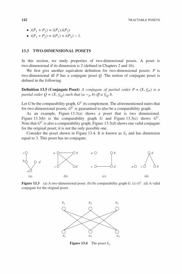
142 TRACTABLE POSETS
• i(P1 + P2) = i(P1).i(P2)• i(P1 ∗ P2) = i(P1) + i(P2) − 1.
13.3 TWO-DIMENSIONAL POSETS
In this section, we study properties of two-dimensional posets. A poset istwo-dimensional if its dimension is 2 (defined in Chapters 2 and 16).
We first give another equivalent definition for two-dimensional posets: P istwo-dimensional iff P has a conjugate poset Q. The notion of conjugate poset isdefined in the following.
Definition 13.5 (Conjugate Poset) A conjugate of partial order P = (X,≤P) is apartial order Q = (X,≤Q) such that (a ∼P b) iff a ||Q b.
Let G be the comparability graph, GC its complement. The aforementioned states thatfor two-dimensional posets, GC is guaranteed to also be a comparability graph.
As an example, Figure 13.3(a) shows a poset that is two dimensional.Figure 13.3(b) is the comparability graph G and Figure 13.3(c) shows GC.Note that GC is also a comparability graph. Figure 13.3(d) shows one valid conjugatefor the original poset; it is not the only possible one.
Consider the poset shown in Figure 13.4. It is known as S3 and has dimensionequal to 3. This poset has no conjugate.
a
c d
b
a
b
c
d
a
c d
b
a c b
d
(a) (b) (c) (d)
Figure 13.3 (a) A two-dimensional poset. (b) Its comparability graph G. (c) GC. (d) A validconjugate for the original poset.
b3
a1 a2 a3
b2b1
Figure 13.4 The poset S3.

TWO-DIMENSIONAL POSETS 143
Yet, another characterization of two-dimensional posets is based on nonseparatinglinear extensions.
Definition 13.6 (Nonseparating Linear Extension) A linear extension L = (X,≤L)of a partial order P = (X,≤P) is called a nonseparating linear extension (NSLE) if
(u ≤L 𝑤 ≤L 𝑣) ∧ (u ≤P 𝑣) ⇒ (u ≤P 𝑤) ∨ (𝑤 ≤P 𝑣).
Figure 13.5(a) shows an NSLE, and a poset (b) corresponding to it. The dottedlines show the possible relationships among u, 𝑣, and 𝑤. At least one of the dottedlines must represent a true edge in order for (a) to be an NSLE of Figure 13.5(b).
We now have the following result.
Theorem 13.7 The following statements are equivalent:
1. P is two dimensional.
2. The incomparability graph of P is a valid comparability graph of some poset.
3. P has a conjugate Q.
4. P has an NSLE.
5. P can be identified with a permutation.
We illustrate Theorem 13.7 with an example taken from Mohring [Moh89] anduse this example to sketch the proof of the theorem. Consider the poset shown inFigure 13.6. The following two linear extensions are such that their intersection givesback the poset P.L1 = 𝑣1 < 𝑣4 < 𝑣2 < 𝑣5 < 𝑣6 < 𝑣3 < 𝑣7L2 = 𝑣3 < 𝑣2 < 𝑣7 < 𝑣1 < 𝑣6 < 𝑣4 < 𝑣5.
ν
w
(a) (b)
u
v
u
w
Figure 13.5 (a) is a non-separating linear extension of the partial order (b), when at least oneof the dotted edges holds.

144 TRACTABLE POSETS
υ1
υ4
υ5 υ6 υ7
υ2 υ3
Figure 13.6 A two-dimensional Poset P = (X,≤P).
υ1
υ2
υ7υ3
υ4 υ5
υ6
Figure 13.7 Conjugate Q = L1 ∩ L2−1 of the poset P.
{L1, L2} is called realizer of P. Note that for every incomparable pair (a, b) in P,if a < b in L1, then b < a in L2.
We can derive the conjugate Q of P from L1 ∩ L2−1, where L2−1 is the total orderderived by reversing the order of the elements in L2.L2−1 = 𝑣5 < 𝑣4 < 𝑣6 < 𝑣1 < 𝑣7 < 𝑣2 < 𝑣3.
Figure 13.7 shows the poset Q that is the conjugate of P obtained from L1 ∩ L2−1.We now show that:
(x ∼P y) ⇔ (x ||Q y)
Since L1 and L2 are linear extensions of P, we have
(x ≤P y) ⇒ (x ≤L2 y) ∧ (x ≤L1 y).
Therefore,y ≤L2−1 x.
Since Q = L1 ∩ L2−1, we get x ||Q y. Similarly, if y ≤P x, then y ||Q x.Now, let P = (X,≤P) be a two-dimensional poset with conjugate Q = (X,≤Q).
Then, ≤P ∪ ≤Q defines a total order on the elements of X.

COUNTING IDEALS OF A TWO-DIMENSIONAL POSET 145
υ1
υ4
υ5 υ6 υ7
υ2 υ3
Figure 13.8 The order imposed by ≤P ∪ ≤Q.
Lemma 13.8 (X,≤P ∪ ≤Q) is an NSLE of P.
Proof: Left as an exercise.
Continuing with our example, Figure 13.8 shows the order imposed by(X,≤P ∪ ≤Q). Figure 13.8 uses directed edges to indicate the ≤ relation. Thenonseparating linear extension consistent with the Figure is:𝑣1 < 𝑣4 < 𝑣2 < 𝑣5 < 𝑣6 < 𝑣3 < 𝑣7.
Note that every linear extension of P is not an NSLE. For example, the followingis a valid linear extension of P, but is not an NSLE:𝑣1 < 𝑣3 < 𝑣4 < 𝑣2 < 𝑣5 < 𝑣6 < 𝑣7.
Finally, we show that every two-dimensional poset P can be identified with apermutation. Let L1 and L2 be the two linear extensions in a minimal realizer ofP, where |P| = n. We can rename the elements of P in such a way that L1 is just[𝑣1, 𝑣2, 𝑣3, ...., 𝑣n]. The position of these elements in the other linear extension, L2,then defines a permutation on [n].
13.4 COUNTING IDEALS OF A TWO-DIMENSIONAL POSET
We now give an efficient algorithm to compute the number of order ideals of atwo-dimensional poset. Assume that we are given the following:
• A two-dimensional poset P = (V ,≤P), and
• L: an NSLE of P
Let L = [𝑣1, 𝑣2, 𝑣3, ..., 𝑣n]. We assign a label, L(𝑣i), to each element 𝑣i, as follows:
L(𝑣1) = 1
L(𝑣i) = 1 +∑
j<i, 𝑣i||𝑣j
L(𝑣j).

146 TRACTABLE POSETS
Given the value of all labels, we can compute the number of nonempty order idealsof P as
N(P) =n∑
i=1
L(𝑣i).
We illustrate the labeling scheme by means of an example. Consider the poset inFigure 13.9. Note that this poset is isomorphic to the one presented in Figure 13.6,but with a different numbering for the nodes. As noted in the figure, the following isan NSLE for the given poset:𝑣1 < 𝑣2 < 𝑣3 < 𝑣4 < 𝑣5 < 𝑣6 < 𝑣7.
By our labeling scheme, we assign the following labels to the nodes in P.L(𝑣1) = 1
L(𝑣2) = 1 + 0 = 1 {since 𝑣1 ∦ 𝑣2 }L(𝑣3) = 1 + L(𝑣1) + L(𝑣2) = 3 {since 𝑣1 ∥ 𝑣3, 𝑣2 ∥ 𝑣3}L(𝑣4) = 1 + 0 = 1 {since 𝑣4 ∦ {𝑣1, 𝑣2, 𝑣3}}L(𝑣5) = 1 + L(𝑣4) + L(𝑣2) = 3 {since 𝑣4 ∥ 𝑣5, 𝑣2 ∥ 𝑣5}L(𝑣6) = 1 + L(𝑣1) + L(𝑣2) + L(𝑣3) + L(𝑣4) + L(𝑣5)
= 10{since {𝑣1, 𝑣2, 𝑣3, 𝑣4, 𝑣5} ∥ 𝑣6}L(𝑣7) = 1 + L(𝑣1) + L(𝑣2) + L(𝑣4) + L(𝑣5) = 7 {since {𝑣1, 𝑣2, 𝑣4, 𝑣5} ∥ 𝑣7}
The following lemma is left as an exercise.
Lemma 13.9 L(𝑣i) is equal to the number of ideals containing 𝑣i and possibly someelements 𝑣j with j < i. N(P) equals the number of nonempty ideals of P.
υ1
υ2
υ4 υ5 υ7
υ3 υ6
Figure 13.9 A partial order P that has a nonseparating linear extension.

BIBLIOGRAPHIC REMARKS 147
13.5 PROBLEMS
13.1. Show that the problem of recognizing any special class of posets that can becharacterized by a constant number of forbidden posets is in complexity classNC.
13.2. Give a (recursive) formula for l(P), the number of linear extensions of an SPorder P.
13.3. Prove Lemma 13.8.
13.4. Prove Lemma 13.9.
13.6 BIBLIOGRAPHIC REMARKS
The reader will find a more detailed discussion of computationally tractable posetsin the survey paper by Möhring [Moh89].

14ENUMERATION ALGORITHMS
14.1 INTRODUCTION
The number of ideals of a poset may be exponential in the size of the poset. We havealready seen that the ideals of a poset form a distributive lattice under the⊆ relation. Inthis chapter, we explore different ways in which the lattice of ideals may be traversed,in order to enumerate all the ideals of a poset.
We explore the following three orders of enumeration:
• Breadth-first search(BFS): This order of enumeration corresponds to the BFStraversal of the lattice of ideals.
• Depth-first search(DFS): This order corresponds to the DFS traversal of thelattice of ideals.
• Lex order: This order corresponds to the “dictionary” order.
We first illustrate the above-mentioned three orders of enumeration by means ofan example. Consider the poset shown in Figure 14.1(a). Figure 14.1(b) shows thelattice of ideals corresponding to this poset. In this figure, we have used the first digitand the second digit to indicate the number of events included in the ideal from thefirst chain and the second chain, respectively. For example, the ideal {e1, e2, f1} isdenoted by 21.
We also give an efficient algorithm to enumerate lexally the level set of the ideallattice for any given level. This algorithm takes time proportional to the number ofelements in that level and not the entire lattice.
In Chapter 11, we have shown that many families of combinatorial objects can bemapped to the lattice of order ideals of appropriate posets. Thus, algorithms for lex
Introduction to Lattice Theory with Computer Science Applications, First Edition. Vijay K. Garg.© 2015 John Wiley & Sons, Inc. Published 2015 by John Wiley & Sons, Inc.
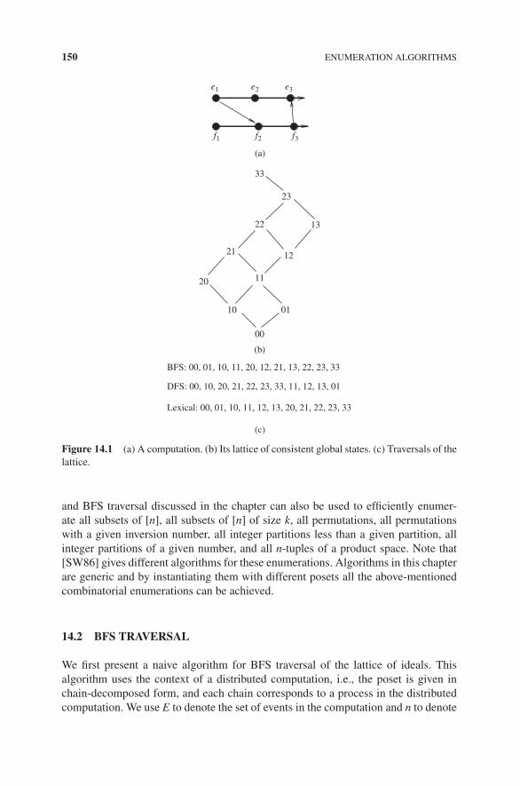
150 ENUMERATION ALGORITHMS
BFS: 00, 01, 10, 11, 20, 12, 21, 13, 22, 23, 33
DFS: 00, 10, 20, 21, 22, 23, 33, 11, 12, 13, 01
Lexical: 00, 01, 10, 11, 12, 13, 20, 21, 22, 23, 33
(c)
(b)
00
10 01
1120
21 12
22 13
23
33
e1 e2 e3
f1 f2 f3
(a)
Figure 14.1 (a) A computation. (b) Its lattice of consistent global states. (c) Traversals of thelattice.
and BFS traversal discussed in the chapter can also be used to efficiently enumer-ate all subsets of [n], all subsets of [n] of size k, all permutations, all permutationswith a given inversion number, all integer partitions less than a given partition, allinteger partitions of a given number, and all n-tuples of a product space. Note that[SW86] gives different algorithms for these enumerations. Algorithms in this chapterare generic and by instantiating them with different posets all the above-mentionedcombinatorial enumerations can be achieved.
14.2 BFS TRAVERSAL
We first present a naive algorithm for BFS traversal of the lattice of ideals. Thisalgorithm uses the context of a distributed computation, i.e., the poset is given inchain-decomposed form, and each chain corresponds to a process in the distributedcomputation. We use E to denote the set of events in the computation and n to denote

BFS TRAVERSAL 151
the number of processes. As we have seen earlier, ideals of the poset correspondto consistent global states(CGSs) in the distributed computation. Throughout thischapter, we use order ideals and CGSs interchangeably.
We keep two lists of CGSs: last and current. Initially, current has the initial CGS.To generate the next level of consistent global states, we set last to current and currentto the set of global states that can be reached from last in one transition. Since a CGScan be reached from multiple global states, an implementation of this algorithm willresult in either current holding multiple copies of a CGS or added complexity in thealgorithm to ensure that a CGS is inserted in current only when it is not present. Thisproblem occurs because the algorithm does not exploit the fact that the set of globalstates forms a distributive lattice.
We now show a method which ensures that a CGS is enumerated exactly once andthat there is no overhead of checking that the CGS has already been enumerated (orinserted in the list). Our extension exploits the following observation.
Lemma 14.1 If H is reachable from G by executing an event e and there exists anevent f ∈ H such that f is maximal in H, then there exists a CGS G′ at the same levelas G such that G′ = G − {f } + {e} and H is reachable from G′.
Proof: Since f is a maximal event in H, it is also a maximal event in G. Since G isconsistent and f is a maximal event in G, it follows that G − {f } is a CGS. Since eand f are both maximal in H, they must be concurrent. If e is enabled at G and f isconcurrent with e, then e is also enabled at G − {f }. Therefore, G′ = G − {f } + {e}is a CGS. H is reachable from G′ on executing f .
Let 𝜎 be a topological sort of all events E in the computation that maps every evente to 𝜎(e) a number from 1..|E|. To avoid enumerating a global state H multiple times,it is sufficient to explore execution of events only in the order consistent with 𝜎. Thus,an event e is explored from a global state G iff e is bigger than all the events in G. Lete be any enabled event in G. We explore execution of e on G iff
∀f ∈ G ∶ 𝜎( f ) < 𝜎(e).
With this observation, our algorithm is shown in Figure 14.2. It keeps a queue Q ofthe CGS. At every iteration, it removes the CGS G at the head of the queue, visits G,and then inserts those successors of G that satisfy the above-mentioned rule.
We now show the correctness of the BFS enumeration algorithm.
Theorem 14.2 Algorithm in Figure 14.2 enumerates every CGS exactly once.
Proof: The proof is by induction on the size of the CGS. The base case holds becausethe empty global state is enumerated exactly once. Let H be any CGS with k events.Let e be the largest maximal event (in the order given by 𝜎). Consider the CGS G =H − {e}. By induction, G is enumerated exactly once. Whenever G is enumerated, His put in the queue Q because e is larger than all events in G.

152 ENUMERATION ALGORITHMS
varQ: set of CGS at the current level initially {(0, 0,… , 0)};𝜎: a topological sort of the poset P;
while (Q ≠ ∅) doG ∶= remo𝑣e−first(Q);enumerate(G);// generate CGS at the next levelfor all events e enabled in G do
if (∀f ∈ maximal(G) ∶ 𝜎(f ) < 𝜎(e)) thenH ∶= G ∪ {e};append(Q,H);
endfor;endwhile;
Figure 14.2 BFS enumeration of CGS.
H cannot be enumerated more than once. Consider any CGS G′ different from Gbut at the same level as G. It can be written as H − {f } for some f different from e.G contains f and e is still explored; therefore 𝜎(f ) < 𝜎(e). However, this implies thatwe will not add H to the queue Q when exploring G′ because f is smaller than theevent e that exists in G′.
We now give a more detailed implementation of the algorithm based on vectorclocks which achieves the time complexity of O(nM), where n is the number of pro-cesses (or width of the poset) and M is the number of ideals of the poset. In theimplementation shown in Figure 14.3, a CGS is represented using the vector clock.For any global state G, we keep the following information.
1. G.state: the vector clock corresponding to the global state G. G.state[i] equalsthe number of events executed on process Pi.
2. G.pred: the predecessor information for the next event on each process.G.pred[i] equals the number of processes that must execute at least one eventbefore the next event on Pi is enabled. The next event on Pi is enabled iffG.pred[i] equals 0.
3. G.admissible: the subset of enabled events that can be explored so that no globalstate is reached twice. An index i ∈ G.admissible iff the next event e on Pi isenabled and 𝜎(e) is greater than 𝜎(f ) for any event that has been executed toreach G.

BFS TRAVERSAL 153
varQ: linked list of CGS at the current level initially empty;G: {state: integer vector, pred: integer vector, admissible: list of indices};∀j ∶ G.state[j] ∶= 0;compute G.pred;G.admissible ∶= {j|(G.pred[j] = 0)};Q.add(G);while (Q is not empty)
G := remove_First(Q);enumerate(G.state);forall (k ∈ G.admissible)
H ∶= G;H.state[k] + +; // execute ek, the admissible event on Pkforall (j ∶ j ≠ k)
// if the next event ej on G[j] depends on ekif (ej.V[k] = H.state[k]) then
H.pred[j] ∶= H.pred[j] − 1;endfor;fk.V = vector clock of the next event on process k;forall (j ∶ j ≠ k)
if (fk.V[j] > G[j]) then H.pred[k] + +;endfor;H.admissible ∶= {j | (H.pred[j] = 0) ∧ (𝜎(ej) > 𝜎(ek))};Q.append(H);
endfor;endwhile;
Figure 14.3 A vector clock based BFS enumeration of CGS.
In the initial state, G.state is a zero vector. We compute G.pred[j] for each j byusing the vector clock information for the next event on each process j. Initially, allenabled events are also admissible since G corresponds to the empty set of eventsexecuted so far.
In the while loop of the algorithm, we remove one global state G from Q andexplore all admissible events from G. The new global state reached on executing thenext event, ek on Pk is called H. We then update H.pred based on the vector clockof ej for next events of all other processes Pj. We also set H.admissible[j] to true iff(H.pred[j] = 0) and 𝜎(ej) > 𝜎(ek). Since we have executed ek on Pk, the next eventon Pk has changed and we recompute the value of H.pred[k] by using the vectorclock for the next event fk (after ek) on Pk. Now we have all the information for H,H.state,H.pred, and H.admissible, and we append it to Q for exploration.
We now analyze the time complexity of the above-mentioned algorithm. We deter-mine the amount of work done before any global state H is inserted in Q. We need

154 ENUMERATION ALGORITHMS
to update H.state,H.pred, and H.admissible before inserting H. This update requiresO(n) time for every global state inserted in Q. Every CGS is inserted in Q exactlyonce giving us the overall time complexity of O(nM).
We now compute the space complexity of the algorithm. The space required ismainly for the linked list Q. Let the width of the lattice of the CGS be 𝑤L. Then,the number of CGS in Q at any time in the algorithm is proportional to 𝑤L. EachCGS requires O(n) storage giving us the overall space complexity of O(n𝑤L) integersassuming that every component of the state vector can be represented by an integer.
The main disadvantage of the above-mentioned algorithm is that it requires spaceat least as large as the number of CGSs in the largest level set. Note that the largestlevel set is exponential in n and therefore when using this algorithm for a large systemwe may run out of memory.
14.3 DFS TRAVERSAL
We now show an algorithm that requires only O(|E|) space. If we traverse ideals inthe DFS order instead of the BFS order, then the number of CGS we have to store inthe worst case is equal to the height of the lattice rather than the width of the lattice.This is a major advantage because the width of the ideal lattice may be exponentiallybigger than its height. The height of the ideal lattice is always |E|, the number ofevents in the poset. In addition, when we traverse the lattice in the DFS order, wealways consider global states G and H that differ by exactly one event. When weexplore H from G by executing an event ek on Pk, we can determine the new globalstate H by advancing along G[k]. When we are done exploring the global state Hand are ready to return to the global state G from H, we can simply decrement H[k]to get G[k]. This incremental feature allows us to avoid storing G.state,G.pred, andG.admissible as required in the BFS algorithm.
To traverse in DFS manner, we show a recursive method in Figure 14.4. The proce-dure dfsTra𝑣ersal is initially called with process indices of all events that are enabledat the initial global state. We keep the global state G and pred as global variables thatare updated as we make the recursive call. We explore an admissible event e on pro-cess Pk from the global state G by calling dfsTraversal(k). Since we are advancing onPk, we recompute pred[k] with O(n) complexity. Next, we decrement pred[j] for allPj such that their next event ej depends on e. Now, we recursively call dfsTra𝑣ersal(j)on all j such that ej is admissible. Once we are done with all the recursive calls, werestore the value of G and pred. This can also be done in O(n) time. Since we takeO(n) time for each recursive call and there are M ideals, the time complexity of thealgorithm is O(nM). The total space requirement for DFS traversal is O(|E|).
14.4 LEX TRAVERSAL
Lex traversal is the natural dictionary order used in many applications. It is impor-tant in many combinatorics applications where combinatorial structures (such as allsubsets of [n] of size k) are ordered in the lex order. Even in distributed computing

LEX TRAVERSAL 155
varG: array[1..n] of integer;pred: array[1..n] of integer;
procedure dfsTra𝑣ersal(int k)let e be the event that is executed on Pk;G[k] + +;enumerate(G);
//compute pred[j] for j ≠ k;forall (j ∶ j ≠ k) with the next event ej on Pj
if ej depends on e then pred[j] − −;
//compute pred[k] using the vector clock for ek, the next event on Pk;ek.V = vector clock of the next event on process k;forall (j ∶ j ≠ k)
if (ek.V[j] > G[j]) then pred[k] + +;
forall (j) with next event ejif (pred[j] = 0) and 𝜎(e) < 𝜎(ej))
dfsTra𝑣ersal(j);
// restore values of G and predforall (j ∶ j ≠ k) with the next event ej on Pj
if ej depends on e then pred[j] + +;G[k] − −;pred[k] = 0;
Figure 14.4 A vector clock based DFS enumeration of CGS.
applications, the user may be interested in the CGS that satisfies the predicate to beminimal with respect to some order. The lex order gives a total order on the set ofCGS based on priorities given to processes and the CGS detected by this traversalgives the lexically smallest CGS.
It is useful to impose on the set of global states the lex or the dictionary order. Wedefine the lex order (<l) as follows. G <l H iff
∃k ∶ (∀i ∶ 1 ≤ i ≤ k − 1 ∶ G[i] = H[i]) ∧ (G[k] < H[k]).
This imposes a total order on all global states by assigning higher priority tosmaller numbered processes. For example, in Figure 14.1, global state (01) <l (10)because P1 has executed more events in the global state (10) than in (01).

156 ENUMERATION ALGORITHMS
We use ≤l for the reflexive closure of the <l relation. Recall that we have earlierused the order ⊆ on the set of global states, which is a partial order. The ⊆ ordershown in Figure 14.1(b) is equivalent to
G ⊆ H ≡ ∀i ∶ G[i] ≤ H[i].
Note that 01 ⊈ 10 although 01 ≤l 10.We now have two orders on the set of global states—the partial order based on con-
tainment (⊆) and the total order based on lex ordering (≤l). The relationship betweenthe two orders defined is given by the following lemma.
Lemma 14.3 ∀G,H ∶ G ⊆ H ⇒ G ≤l H.
Proof: G ⊆ H implies that ∀i ∶ G[i] ≤ H[i]. The lemma follows from the definitionof the lex order.
Since there are two orders defined on the set of global states, to avoid confusionwe use the term least for infimum over ⊆ order, and the term lexically minimum forinfimum over the ≤l order.
Let nextLex(G) denote the CGS that is the successor of G in the lex order. Forexample, in Figure 14.1, nextLex(01) = 10 and nextLex(13) = 20. It is sufficient toimplement nextLex function efficiently for enumeration of ideals in the lex order.One can set G to the initial CGS ⟨0, 0, ..., 0⟩ and then call the function nextLex(G)repeatedly. We implement the function nextLex(G) using two secondary functionssucc and leastConsistent as described in the following.
We define succ(G, k) to be the global state obtained by advancing along Pk andresetting components for all processes greater than Pk to 0. Thus, succ(⟨7, 5, 8, 4⟩, 2)is ⟨7, 6, 0, 0⟩ and succ(⟨7, 5, 8, 4⟩, 3) is ⟨7, 5, 9, 0⟩. Note that succ(G, k) may not existwhen there is no event along Pk, and even when it exists, it may not be consistent.
The second function is leastConsistent(K) that returns the least CGS greater thanor equal to a given global state K in the ⊆ order. This is well defined because the setof all consistent global states that are greater than or equal to K in the CGS lattice isa sublattice.
We now show how nextLex(G) can be computed.
Theorem 14.4 Assume that G is a CGS such that it is not the greatest CGS. Then,
nextLex(G) = leastConsistent(succ(G, k)),
where k is the index of the process with the smallest priority, which has an eventenabled in G with respect to all higher priority processes.
Proof: We define the following global states for convenience:K ∶= succ(G, k)H ∶= leastConsistent(K), and

LEX TRAVERSAL 157
G′ ∶= nextLex(G).Our goal is to prove that G′ = H.
G′ contains at least one event f that is not in G; otherwise G′ ⊆ G and thereforecannot be lexically bigger. Choose f ∈ G′ − G from the highest priority process pos-sible.
Let e be the event in the smallest priority process enabled in G, i.e., e is on processPk. Let proc(e) and proc(f ) denote the process indices of e and f . We now do a caseanalysis.
Case 1: proc(f ) < proc(e)In this case, e is from a lower priority process than f . We show that this case impliesthat H is lexically smaller than G′. We first claim that H ⊆ G ∪ {e}. This is becauseG ∪ {e} is a CGS containing K and H is the smallest CGS containing K. Now, sinceH ⊆ G ∪ {e} and G′ contains an event f ∈ G′ − G from a higher priority processthan e, it follows that H is lexically smaller than G′, a contradiction.
Case 2: proc(f ) > proc(e)Recall that event e is on the process with the smallest priority that had any eventenabled at G with respect to all higher priority processes. Therefore, existence of fin CGS G′ implies existence of at least another event, say f ′ in G′ − G at a processwith priority than at least equal to that of e (otherwise, we contradict the choiceof e). However, existence of f ′ ∈ G′ − G contradicts choice of event f because, bydefinition, f is from the highest priority process in G′ − G and priority of f ′ is greaterthan priority of f .
Case 3: proc(f ) = proc(e).Then, K ⊆ G′ because both G′ and K have identical events on Pk and processes withhigher priority and K has no events in lower priority processes. Since G′ is a CGSand K ⊆ G′, we get that H ⊆ G′ by definition of H. From Lemma 14.3, it followsthat H ≤l G′. But G′ is the next lexical state after G. Therefore, H = G′.
The only task left in the design of the algorithm is to determine k and implementleastConsistent function. The following lemma follows from properties of vectorclocks. First, we determine that an event e in enabled in a CGS G if all the componentsof the vector clock for other processes in e are less than or equal to the componentsof the vector clock in G. Secondly, to compute leastConsistent(K), it is sufficient totake the component-wise maximum of the vector clock of all maximal events in K.Formally,
Lemma 14.5
1. An event e on Pk is enabled in a CGS G iff e.𝑣[k] = G[k] + 1 and
∀j ∶ j ≠ k ∶ e.𝑣[j] ≤ G[j].

158 ENUMERATION ALGORITHMS
Lex()
Input: a poset P with any partition 𝛼 into chains P1, ..PnOutput: All ideals in lexical ordervar
G:array[1 …n] of int initially ∀i ∶ G[i] = 0; // current ideal(1) enumerate(G);(2) while (true)(3) for k ∶= n down to 1 do(4) if (next element on Pk exists)(5) if (next element on Pk enabled for P1..Pk−1) break;(6) if no such k, then return;// we have enumerated all tuples(7) G[k] ∶= G[k] + 1;(8) for i ∶= k + 1 to n do // reset lexically smaller components(9) G[i] ∶= 0;(10) // ensure that G is an ideal(11) for i ∶= 1 to k such that G[i] ≠ 0 do // include in G all
smaller elements(12) for j ∶= k + 1 to n do(13) G[j] ∶= max(G[i].V[j],G[j]);(14) enumerate(G);(15) endwhile;
Figure 14.5 An algorithm for lexical traversal of all ideals of a poset with any chain partition.
2. Let H = leastConsistent(K). Then,
∀j ∶ H[j] = max{K[i].𝑣[j] | 1 ≤ i ≤ n}.
Incorporating these observations, we get the algorithm in Figure 14.5.The algorithm in Figure 14.5 enumerates all ideals in the lexical order assuming
that the poset P is in the chain partitioned form. Line (1) enumerates the least idealin lexical order, which is always (0, 0, ..0). The variable G is set to this value andenumerated at line (1). The while loop (lines (2) to (15)), enumerates the next lexicallybigger ideal than G whenever possible. The for loop (lines (3)–(5)) finds the largestk such that the next element on Pk is such that all elements in P1..Pk−1 smaller thanthat element are included in G. Formally, we say that element e is enabled in an idealG iff
∀f ∈ P ∶ f < e ⇒ f ∈ G.
An element e is enabled in an ideal G with respect to Pi if
∀f ∈ Pi ∶ f < e ⇒ f ∈ G.

LEX TRAVERSAL 159
Therefore, e is enabled in G for P1..Pk−1 iff
∀i ∶ 1 ≤ i < k ∶ e.V[i] ≤ G[i].
If we do not find any k, then we must have enumerated all ideals and we break thewhile loop at line (6). We include the next element at Pk in G at line (7). We removeall elements in chains Pk+1 to Pn at lines (8) and (9). Observe that G now containselements only from chains P1 to Pk. Lines (11)–(13) now ensure that G is an idealby including sufficient elements from Pk+1 to Pn. If G[i] is not equal to zero for anyi ∈ {1..k}, we include all elements in G[i].V .
For an example of this algorithm, consider the poset L(3, 3) shown in Figure 14.6.Suppose that the last subset enumerated was G = [1, 1, 0] also shown in the figure.For the next ideal, we start with P3. The next element on P3 (the element e3,1) isconsidered for inclusion. It is enabled with respect to P1 and P2 because elementsthat are smaller than this element in P1 and P2 are already included in G. Hence,after line (9), G is [1, 1, 1]. Since k is 3, lines (10)–(13) do not change anything andthe following subset enumerated is [1, 1, 1]. Now consider the next iteration of thewhile loop. We first check if the second element on P3 is enabled. This is not the casesince the second element on P3 is greater than the second element on P2, which isnot included in G. Next, we try the second element on P2. However, that element isalso not enabled. Next, we try the second element on P1 which is enabled. Hence, weget G as [2, 1, 1]. We now reset the components for processes with higher indices atlines (8) and (9). After the resetting of components, G is [2, 0, 0] and is enumeratednext. Note that even for this case, lines (10)–(13) do not change G. The algorithmcontinues to enumerate ideals as [2, 1, 0], [2, 1, 1], [2, 2, 0], and so on.
Let us analyze the time complexity of Algorithm Lex. We compute the timerequired for enumeration of one ideal. Every iteration of the while loop enumeratesone ideal. Line (4) requires determining if the next element on Pk in G exists andline (5) checks if that event is enabled for P1..Pk−1. The next element on Pk exists iffG[k] is less than the total number of elements in Pk, a condition that can be evaluatedin O(1) time. Let e be the next element on Pk in G. As mentioned earlier, it is enabledin G for P1..Pk−1 iff
1
32
21
2
0
0
0
3
3
1
Figure 14.6 L(3, 3) with example of an ideal.

160 ENUMERATION ALGORITHMS
∀i ∶ 1 ≤ i < k ∶ e.V[i] ≤ G[i].
This condition can be evaluated in O(k) time. Therefore, the Algorithm Lex requiresO(n2) for enumeration of one ideal at line (5). Lines (11)–(13) also require O(n2) timegiving us the overall complexity of O(n2) time per ideal.
14.5 UNIFLOW PARTITION OF POSETS
We describe in this section a special type of chain partition called uniflow chain parti-tion that allows efficient enumeration of ideals and ideals at a given level. Every posetP has at least one such partition. Let n be the least number of chains in any uniflowchain partition of P. We present two algorithms in this section. The first algorithmenumerates all the ideals of a poset with a uniflow chain partition. It takes O(n2) timeper ideal to enumerate the set of ideals of P. By considering special properties of theposet P, the time complexity can be reduced to O(n) for many applications in com-binatorics. The second algorithm enumerates all the ideals at a given level of a posetwith a uniflow chain partition. This algorithm takes O(n3) time per ideal to enumeratethe set of ideals of size k of poset P. Furthermore, the algorithm requires only O(n)space in addition to the storage required for storing the poset.
A uniflow partition of a poset P is a partition of P into n chains {Pi | 1 ≤ i ≤ n}such that no element in a higher numbered chain is smaller than any element in lowernumbered chain. Formally, let 𝛼 ∶ P → ℕ be a chain partition of P, i.e., 𝛼 maps everyelement of P to a natural number such that
∀x, y ∈ P ∶ 𝛼(x) = 𝛼(y) ⇒ (x ≤ y) ∨ (y ≤ x).
A chain partition 𝛼 is uniflo𝑤 for a poset if
∀x, y ∈ P ∶ 𝛼(x) < 𝛼(y) ⇒ ¬(y ≤ x). (14.1)
Figure 14.7(a) shows an example of the partitioned poset L(n,m) with n chainseach of m elements. In L(n,m), element j of chain Pi is smaller than element j of allhigher numbered chains. If chains are arranged from top to bottom such that the leastnumbered chain is at the top, then all edges across chains in a uniflow partition goin one direction. Figure 14.7(b) shows L(3, 3). The dashed line shows an ideal of theposet. All the elements of the poset that are to the left of the dashed line are membersof the ideal. In Figure 14.7(b), the ideal contains one element from P1, one elementfrom P2, and no element from P3. Each ideal of L(3, 3) can be mapped to a subset of[6] of size 3 as follows. To choose a subset S of size 3, we use the number of elementsof each chain included in the ideal. The number of elements included in P1 dictatesthe largest number in S, the number of elements included in P2 dictates the secondlargest number, and so on. If P1 has k elements in the ideal, then we include 3 + kin S. Since the ideal in the figure includes one element from P1, we include 4 in S.

UNIFLOW PARTITION OF POSETS 161
(a)(b)
654
43
432
2
1
3
5
P1
P2
Pn
en,1
e1,1e1,m
en,m
Figure 14.7 (a) Poset L(n,m) with uniflow partition. (b) L(3, 3) with an example of an idealmapped to the subset {1, 3, 4}.
Similarly, we include 3 in S because one element from P2 is included and include 1 inS because zero elements from P3 are included. Thus, the ideal in the figure denotes thesubset {1, 3, 4} of [6]. We have labeled edges in Figure 14.7(b) to show the bijectionbetween ideals and subsets of [6] of size 3.
Another example of a poset with uniflow partition is shown in Figure 14.8. Thepartitioned poset D(n,m) consists of n disjoint chains each with m elements. Figure14.8(b) shows D(3, 3). For this example, the uniflow condition holds trivially becauseelements on distinct chains are incomparable. Each ideal of this poset corresponds toa tuple in the product space of 64 tuples from (0, 0, 0) to (3, 3, 3).
Figure 14.9(a) shows a chain partition that does not satisfy the uniflow property.The same poset can be partitioned into three chains with the uniflow property asshown in Figure 14.9(b). Note that every poset has at least one uniflow chain parti-tion. Any linear extension can be transformed into a trivial uniflow chain partition byconsidering each element as a chain by itself.
In our definition of uniflow poset, we require that no element in a higher numberedchain be smaller than any element in a lower numbered chain. By renumbering the
321
21
0
0 3
0 1 2 3P1
P2
Pnen,1
e1,m
en,m
e1,1
(a) (b)
Figure 14.8 (a) Poset D(n,m) with uniflow partition (b) D(3, 3) with example of an ideal.

162 ENUMERATION ALGORITHMS
h
e
f
g
(b)
g h
e f
(a)
P1P1
P2
P3
P2
Figure 14.9 (a) Chain partition of a Poset that is not uniflow. (b) Uniflow chain partition ofthe same poset.
chains, any such poset also has a chain partition 𝛽 with the dual property that
∀x, y ∈ P ∶ 𝛽(y) < 𝛽(x) ⇒ ¬(y ≤ x). (14.2)
We call a chain partition 𝛼 that satisfies Equation 14.1, positive uniflow and a chainpartition 𝛽 that satisfies Equation 14.2, negative uniflow partition.
An advantage of uniflow chain partition is that it allows us to enumerate idealsfrom a given ideal efficiently as shown later.
Lemma 14.6 (Positive Uniflow Ideals Lemma) Let G be any ideal of a poset P witha positive uniflow chain partition {Pi | 1 ≤ i ≤ n}. Any subset Hk of P for 1 ≤ k ≤ nthat satisfies
∀i ∶ 1 ≤ i < k ∶ Hk[i] = G[i]
and∀i ∶ k ≤ i ≤ n ∶ Hk[i] = 0
is also an ideal.
Proof: Follows from Equation 14.1.
For example, in Figure 14.9(b), consider the ideal G = {e, f , g} represented asG = [1, 1, 1] in the uniflow partition. Then, Lemma 14.6 claims that the subsets of Prepresented by [0, 0, 0], [1, 0, 0], [1, 1, 0] are also ideals. The claim may not hold ifthe chain partition does not have uniflow property. For example, in Figure 14.9(a),G = {e, f , g} is represented as G = [2, 1]. However, the set [2, 0] is not an ideal; itincludes f but not g.
We get the following version of the Uniflow ideal lemma with a negative uniflow.
Lemma 14.7 (Negative Uniflow Ideals Lemma) Let G be any ideal of a poset Pwith a negative uniflow chain partition {Pi | 1 ≤ i ≤ n}. Then, any subset Hk of P for1 ≤ k ≤ n that satisfies
∀i ∶ 1 ≤ i ≤ k ∶ Hk[i] = G[i]

ENUMERATING ALL SUBSETS 163
TABLE 14.1 Special cases of lex enumeration of ideals of a poset.
Enumeration Ideals of the Poset
Product space D(n,m) (see Figure 14.8)Subsets of [n] D(n, 1) (see Figure 14.8)Subsets of [m + n] of size n L(n,m) (see Figure 14.7)Permutations of 1..n T(n) (see Figure 14.12)Integer partitions that fit in an n by m rectangle L(n,m) (see Figure 14.7)Catalan subset of [2n] of size n C(n) (see Figure 14.12)
and∀i ∶ k + 1 ≤ i ≤ n ∶ Hk[i] = |Pi|
is also an ideal.
Proof: Follows from Equation 14.2.
We now simplify the algorithm for a positive uniflow chain partition. Owing tothe positive uniflow property of the chain partition, if any element e belongs to thechain k, then any element smaller than e also belongs to a chain numbered k or lower.Hence, lines (10)–(13) in Algorithm Lex() in Figure 14.5 are not necessary owingto Positive Uniflow Ideals Lemma. Similarly, if the chain partition satisfies negativeuniflow property then line (5) in Figure 14.5 is not necessary because for any elemente on chain k, there is no element smaller than e in any chain numbered lower than k(Table 4.1).
14.6 ENUMERATING TUPLES OF PRODUCT SPACES
We first give the most straightforward application to enumeration of combinatorialobjects. We show that we can derive efficient algorithms for many combinatorialobjects such as all subsets of [n], all subsets of [n] of size k, all permutations, andall tuples of product spaces.
Consider a product space (x1, x2, ..., xn) such that each xi ∈ [0..mi]. It is clear thatthe product space has Πi∈1..n](mi + 1) tuples. We can view these tuples as ideals of theposet D(n,m) with the chain partition shown in Figure 14.8. This partition satisfiespositive as well as negative uniflow partitions; hence, we can apply both optimizationsand get the algorithm shown in Figure 14.10.
It is clear that the above-mentioned algorithm produces a new tuple after at mostO(n) steps on account of two for loops at lines 3 and 6.
14.7 ENUMERATING ALL SUBSETS
We now consider the problem of enumerating all subsets of a given finite set. Weshow that there may be multiple posets such that the ideals of the poset are mapped

164 ENUMERATION ALGORITHMS
lexTraverseProductSpace()
Input: [m1,m2, ...,mn] // largest tuple of the product spaceOutput: All tuples in lex ordervar
G:array[1 …n] of int initially ∀i ∶ G[i] = 0; // current CGS(1) enumerate(G);(2) while (true)(3) for k ∶= n down to 1 do(4) if (G[k] < mk) break;(5) if no such k, then return;// we have enumerated all tuples(6) G[k] ∶= G[k] + 1;(7) for j ∶= k + 1 to n do G[j] ∶= 0;(8) enumerate(G);(9) endwhile;
Figure 14.10 An algorithm for traversal of product space in lex order.
in 1-1 manner with subsets. The first method of generating all subsets of the set [n] isto view every subset as a binary string of size n. Enumerating all subsets is equivalentto enumerating all 2n binary strings of size n. However, this is just a special case ofenumerating the product space where each of mk is 1. In this case, the product spacecorresponds to the ideals of the poset shown in Figure 14.11(a). Each process Pi exe-cutes a single event ei. It is easy to verify that there is a bijection between every CGSof the computation and a subset of X. For example, when n = 4, the CGS (0, 1, 0, 1)corresponds to the set {e2, e4}. The lex enumeration would correspond to enumera-tion of sets based on binary string representation. For n equal to 3, the enumerationwould be {}, {1}, {2}, {1, 2}, {3}, {1, 3}, {2, 3}, {1, 2, 3}. Given any subset S, thisenumeration corresponds to the following rule to generate the next subset after S:insert the smallest element j which is not in S and delete all elements smallerthan j.
Figure 14.11(b) gives another computation that can also be used to enumerateall the subsets of {1..4}. In this example, the enumeration would result in the lexorder (reversed). Each global state (or a cut) corresponds to a subset. For example,G corresponds to the subset {4, 2, 1}. We say that Pi has chosen element k if the cut(global state) goes through the label k for process Pi. In this computation, P1 choosesthe biggest element in the set. By the design of the computation, P2 can only choosean element that is strictly smaller than the element chosen by P1 for the global stateto be consistent. For example, the global state H is not consistent because P2 hasalso chosen 1, which is same as the element chosen by P1. The choice of 0 by any

ENUMERATING ALL SUBSETS OF SIZE K 165
(a) (b)
43 2 1 0
3 2 1 0
2 1 0
1 0
G H
e1
e2
e3
en
Figure 14.11 Posets for generating subsets of X.
Pi denotes that the process does not choose any element. It can be verified that if Pichooses 0, then all higher numbered processes can only choose 0.
We leave it as an exercise for the reader to adapt the lex algorithm for traversing aposet with poset uniflow property to enumerate all subsets using the poset in Figure14.11(b).
14.8 ENUMERATING ALL SUBSETS OF SIZE K
Figure 14.7 shows the poset L(n,m) such that all the subsets of [n + m] of size nare in 1-1 correspondence with its ideals. If G[i] is j then we add (j + (n − i + 1)) tothe set. For example, when G = (1, 1, 0), i.e., G[1] = 1, G[2] = 1, and G[3] = 0, weget elements 1 + (3 − 1 + 1), 1 + (3 − 2 + 1), and 0 + (3 − 3 + 1). Thus, the subsetcorresponds to {4, 3, 1}. Figure 14.13 shows the algorithm to generate all ideals ofL(n,m). Since L(n,m) satisfies positive uniflow property, once a suitable k is found atline (4), advancing along G[k] and resetting G[j] to 0 for all chains j numbered higherthan k gives us the next lexically bigger ideal. Line (4) returns the element on highestnumbered chain Pk, which is enabled with respect to P1, ...Pk−1. The first few idealsenumerated for L(3, 3) are
(0, 0, 0), (1, 0, 0), (1, 1, 0), (1, 1, 1), (2, 0, 0), ...
By mapping G[i] to element G[i] + (n − i + 1), we get the subsets
(3, 2, 1), (4, 2, 1), (4, 3, 1), (4, 3, 2), (5, 2, 1).

166 ENUMERATION ALGORITHMS
4
5
6
6
8 9
3
7
5
(a) (b)2
3
4
5
7
Figure 14.12 (a) Poset C(5) with a uniflow partition (b) Poset T(5) with a uniflow partition.
lexTraverseSubsetsOfGivenSize()
Input: n, mOutput: All subsets of [n] of size mvar
G:array[1 …n] of int initially ∀i ∶ G[i] = 0; //(1) enumerate(G);(2) while (true)(3) for k ∶= n down to 1 do(4) if ((k == 1)&&(G[1] < m) || ((k > 1)&&(G[k] < G[k − 1]))) then(5) break; // suitable k found(5) if no such k, then return;// we have enumerated all tuples(6) G[k] ∶= G[k] + 1;(7) for j ∶= k + 1 to n do G[j] ∶= 0;(8) enumerate(G);(9) endwhile;
Figure 14.13 An algorithm for traversal of all subsets of [n] of size m in lex order.
14.9 ENUMERATING YOUNG’S LATTICE
Recall that the set of all partitions that are less than or equal to 𝜆 form the Young’slattice denoted by Y𝜆. Figure 14.14 shows the poset for generating Young’s lattice.By enumerating all ideals of the poset in lex order, we can enumerate all partitionsthat are less than or equal to 𝜆.
Figure 14.15 gives the algorithm to enumerate Y𝜆.Now consider the Young Lattice for 𝜆 = (N,N,…N times). The Nth level set of
this lattice corresponds to all integer partitions of N. By enumerating the Nth level

ENUMERATING PERMUTATIONS 167
(b)(a)
P1
P2
P3
Figure 14.14 (a) A Ferrer’s diagram. (b) A poset for generating Young’s lattice.
lexTraverseYoungLattice()
Input: 𝜆 = (𝜆1,… , 𝜆n)Output: All integer partitions less than or equal to 𝜆
varG:array[1 …n] of int initially ∀i ∶ G[i] = 0; //
(1) enumerate(G);(2) while (true)(3) for k ∶= n down to 1 do(4) if ((k == 1)&&(G[1] < 𝜆1) || ((k > 1)&&(G[k] < G[k − 1])
&& (G[k] < 𝜆k))) then(5) break; // suitable k found(5) if no such k, then return;// we have enumerated all tuples(6) G[k] ∶= G[k] + 1;(7) for j ∶= k + 1 to n do G[j] ∶= 0;(8) enumerate(G);(9) endwhile;
Figure 14.15 An algorithm for traversal of all integer partitions in Y𝜆
in lex order.
set, we can enumerate all integer partitions of N. We discuss algorithms to enumeratelevel sets in the following section.
14.10 ENUMERATING PERMUTATIONS
Finally, we show that our algorithms can also be used to enumerate permutations. Wefirst show a poset such that its ideals can be mapped to all permutations of n symbols.Figure 14.12(b) shows the poset T(n) for n = 5. The poset consists of n − 1 chains.We use the inversion table[Knu98] to map an ideal to a permutation. The number ofinversions of i in a permutation 𝜋 is the number of symbols less than i that appear tothe right of i in 𝜋. The way a permutation is generated from an ideal is as follows. We

168 ENUMERATION ALGORITHMS
begin the permutation by writing 1. P1 decides where to insert the symbol 2. Thereare two choices. These choices correspond to number of inversions introduced by 2.If we place 2 after 1, then we introduce zero inversions; Otherwise, we introduceone inversion. Proceeding in this manner, we get that there is a bijection between theset of permutations and the ideals. By using the algorithm to generate all ideals ofthe product space and converting the ideal viewed as a tuple of inversion number tocorresponding permutation, we get an algorithm to generate all permutations.
In many applications, we are interested in subsets of combinatorial families. Forexample, we may be interested in enumerating all permutations of 1..7 in which 7 hasat most three inversions. By using methods of slicing, one can compute posets suchthat its ideals correspond to precisely this subset. Now we can use the algorithm forlex order traversal to enumerate all such permutations.
14.11 LEXICAL ENUMERATION OF ALL ORDER IDEALS OF A GIVENRANK
Many combinatorial objects have bijections with ideals of a given rank rather thanall ideals. For example, all subsets of [n] of size r can be mapped to level r of theBoolean lattice, which is simply ideals of D(n, 1). As another example, considerthe ideals of L(n, n). It is easy to see that all integer partitions of n have bijection withthe set of ideals of rank n. In this section, we give an efficient algorithm to generate allideals of a given rank. In this section, we assume that the poset is decomposed usinga negative uniflow chain partition. Figure 14.17(a) shows a poset NL(n,m) with anegative uniflow chain partition. Figure 14.17(b) shows a poset NL(3, 3) such that allideals at rank 3 correspond to integer partitions of 3. There are three integer partitionsfor 3
3, 2 + 1, 1 + 1 + 1.
These partitions correspond to the following ideals in the lexical order.
[0, 0, 3], [0, 1, 2], [1, 1, 1].
Note that the indices of the chains are in the reversed order of the conventional way ofwriting integer parts from the greatest to the smallest. The algorithm in Figure 14.16enumerates these partitions in the above-mentioned order.
The algorithm works as follows. We first find the lexically smallest ideal at therequired level r. This step is performed by the method getSmallest(G, r) (shown inFigure 14.18), which returns the lexically smallest ideal of P bigger than G at level r.For example, in Figure 14.17, getSmallest([0, 0, 0], 3) returns the lexically smallestideal [0, 0, 3]. Given an ideal G at level r, we repeatedly find the next lexically biggerideal at level r using the algorithm getSucc(G, r) shown in Figure 14.19. For example,in Figure 14.17, getSucc([0, 0, 3], 3) returns the next lexically smallest ideal [0, 1, 2].
The method getSmallest(G, r) on poset P assumes that the rank of G is at most rand that G is an ideal of the poset P. It first computes d as the difference between

LEXICAL ENUMERATION OF ALL ORDER IDEALS OF A GIVEN RANK 169
LevelTraverse()
Input: P: a poset partitioned into uniflow chains P1, ..Pnr: integer; // a level number
Output: All ideals of P at level r in the lexical ordervar
G: array[1 …n] of int initially ∀i ∶ G[i] = 0; // least ideal(1) G := getSmallest(G, r);(2) while (G ≠ null)(3) enumerate(G);(4) G := getSucc(G, r);(5) endwhile;
Figure 14.16 An algorithm for traversal of a level set in lexical order.
(a)(b)
321
321
321
0
0
0
P1
P2
Pn
e1,m
en,m
Figure 14.17 (a) Poset NL(n,m) with a negative uniflow partition. (b) NL(3, 3) with exampleof an ideal.
r and the rank of G. We need to add d elements to G to find the smallest ideal atrank r. We exploit the negative Uniflow Ideal Lemma (Lemma 14.7) by adding asmany elements from the largest numbered chain as possible. If all the elements fromthe largest numbered chain are already in G, then we continue with the second largestnumbered chain, and so on. For our example in Figure 14.17, consider finding small-est ideal at level 3 starting from G = [0, 0, 0]. In this case, we are done by adding allthree elements from P3 to get the answer as [0, 0, 3].
The following lemma shows that the resulting set is the smallest ideal of rank rand which is greater than or equal to G.
Lemma 14.8 Let G be any ideal of rank at most r. Then, getSmallest(G, r) is lexicallythe smallest ideal of rank r greater than or equal to G.
Proof: Let H be the set returned by getSmallest(G, r). We first show that H is anideal. H is initialized to G which is an ideal. We show that H continues to be an ideal

170 ENUMERATION ALGORITHMS
getSmallest(G,r)
Input: P: a poset partitioned into negative uniflow chains P1, ..Pn;r: integer; // a level numberG: an ideal;
Output: H: lexically smallest ideal at level r greater than or equal to Gvar
H:array[1..n] of int initially ∀i ∶ H[i] = G[i];(1) int d ∶= r − rank(G);(2) for j ∶= n down to 1 do(3) if (d ≤ |Pj| − G[j])(4) H[j] ∶= G[j] + d;(5) return H;(6) else(7) H[j] ∶= |Pj|;(8) d ∶= d − (|Pj| − G[j]);(9) endfor;
Figure 14.18 An algorithm to find the lexically smallest ideal at level r greater than G.
after every iteration of the for loop. At iteration j, we add to H elements from chainn − j + 1. Since all elements from higher numbered chains are already part of H, andall elements from lower numbered chains cannot be smaller than any of the newlyadded element, we get that H continues to be an ideal.
By construction of our algorithm, it is clear that rank of H is exactly r. We nowshow that H is the lexically smallest ideal at rank r greater than or equal to G. If not,let W different from H be the lexically smallest ideal at rank r greater than or equal toG. Since W <l H, let k be the smallest index such that W[k] < H[k]. Since G ≤l W,k is one of the indices for which we have added elements. Because rank of W equalsrank of H, there must be an index k′ higher than k such that W[k′] > H[k′]. However,by the property of H for any index k′ higher than k, H[k′] equals |Pk′ |. Hence, W[k′]cannot be greater than H[k′].
We now discuss the method getSucc(G, r) shown in Figure 14.19. To find the nextlexical ideal of G at level r, we proceed as follows. The for loop (lines (1)–(11))searches for an appropriate element z not in G such that on addition of z, the resultingideal K is guaranteed to be greater than G. The search for z is started from chain ndown to 1 so that we choose the lexically smallest z that is not in G. Line (2) checksif there is any element in Pk. If all elements from Pk are already included in G, wego to the next value of k. Otherwise, in lines (3)–(4), we include in K all elements in

LEXICAL ENUMERATION OF ALL ORDER IDEALS OF A GIVEN RANK 171
getSucc(G, r)
Input: G: Any ideal at level rr: integer; // a level number
Output: Lexical successor of G at level rvar
K:array[1 …n] of int initially ∀i ∶ K[i] = 0;;(1) for k ∶= n down to 1 do(2) if (the next element z on Pk exists)(3) for i ∶= 1 to k − 1: // include in K all elements
from G from P1 to Pk−1(4) K[i] := G[i];(5) K[k] := G[k] + 1;// include the element z(6) // include in K all elements required to make it an ideal(7) for i ∶= 1 to k:(8) for j ∶= k + 1 to n:(9) K[j] := max(K[j],G[i].V[j]);(10) if (rank(K) ≤ r) break ;// found suitable K(11) endfor;(12) if no suitable K then return null;// we have enumerated all tuples(13) else return getSmallest(K, r);
Figure 14.19 An Algorithm to find the next bigger ideal in a level set.
G from chains 1 to k − 1. Line (5) includes in K all elements in G from Pk and z. Toensure that K is an ideal, for every element y in K, we add D[y] to K at lines (7)–(9).At line (10), we check whether the resulting ideal is at level r or less. If rank(K) isat most r, then we have found a suitable K that can be used to find the next lexicallybigger ideal than G and we break the for loop to go to line (13). If we have tried allvalues of k and did not find a suitable K, then G is the largest ideal at level r and wereturn null.
For our example in Figure 14.17, consider the call of getSucc from the ideal [0, 0, 3]for rank 3. Since there is no next element in P3, we consider the next element inP2. At line (5), the value of K is [0, 1, 0]. Lines (7)–(9) make K an ideal resultingin K to be [0, 1, 1] at line (10). Since rank(K) is 2, we break the for loop and callgetSmallest(K, r) to find the smallest ideal at level r that contains K. For our example,we call getSmallest([0, 1, 1], 3) at line (13). The resulting ideal is the lexical successorof G at level r. For our example, this ideal corresponds to [0, 1, 2].
We now show the correctness of the method getSucc(G, r).
Lemma 14.9 Let G be any ideal of rank at most r. Then, getSucc(G, r) returns theleast ideal at rank r that is lexically greater than G.

172 ENUMERATION ALGORITHMS
TABLE 14.2 Special cases of lex enumeration of level sets of the ideal lattice of aposet
Enumeration Poset Level number
Subsets of [n] of size k D(n, 1) (see Figure 14.8) kInteger partitions of n L(n, n) (see Figure 14.7) nAll compositions of n with k parts D(k, n − k) (see Figure 14.8) n − kPermutations of 1..n with k inversions T(n) (see Figure 14.12) k
Proof: Let W be the ideal returned by getSucc(G, r). We consider two cases. Supposethat W is null. This means that for all values of k, either all elements in Pk are alreadyincluded in G or on inclusion of the next element in Pk, z, the smallest ideal thatincludes z has rank greater than r. Hence, G is lexically biggest ideal at level r.
Now consider the case when W is the ideal returned at line (13) bygetSmallest(K, r). We first observe that K after executing line (9) is the next lexicalideal (at any level) after G. If rank(K) is at most r, then getSmallest(K, r) returnsthe smallest lexical ideal greater than or equal to K at level r. If rank(K) is greaterthan r, then there is no ideal at level r such that ∀i ∶ 1 ≤ i ≤ k − 1 ∶ K[i] = G[i] andK[k] > G[k] and rank(K) ≤ r. Thus, at line (13), we use the largest possible value ofk for which there exists an ideal lexically bigger than G at level r.
The algorithm getSucc(G, r) takes O(n3) time in the worst case because of nestedfor loops. We now apply the level enumeration algorithm to various combinatorialfamilies given in Table 14.2.
Theorem 14.10 All subsets of [n], all integer partitions, all compositions of n withk parts, and all permutations with k inversions can be generated in O(n3) time perenumeration by using the LevelTraverse algorithm shown in Figure 14.16.
Proof: It is easy to verify that the level sets of the ideals of the posets listed in Table14.2 correspond to the combinatorial family listed in column 1 of Table 14.2
14.12 PROBLEMS
1. Show that in the algorithm shown in Figure 14.2, if H is inserted as the firstelement in Q, rather than the last element, then the algorithm traverses the latticein the depth-first-search order.
2. Show that in the algorithm shown in Figure 14.2, we can replace the conditionfor exploring e by
∀f ∈ maximal(H) ∶ 𝜎(f ) < 𝜎(e).

BIBLIOGRAPHIC REMARKS 173
3. Give a nonrecursive version of the Algorithm in Figure 14.4 for DFS traversal ofideals.
4. Show that H at line (12) in Figure 14.5 is indeed the next lexical state after G.
5. Show that in Figure 14.5, it is sufficient to take the maximum of G, and the vectorK[k] to compute H whenever the value of k in the current iteration is greater thanor equal to the one in the previous iteration instead of lines (9)–(12).
6. Give an algorithm to generate all partitions of n with at most k parts.
7. Give an algorithm to generate all the subsets of [n] of size k in lexical order whichdo not contain any consecutive numbers.
14.13 BIBLIOGRAPHIC REMARKS
The first algorithm for BFS traversal of the lattice of global states is from Cooperand Marzullo [CM91]. The second algorithm for BFS traversal is taken from Garg[Gar03]. The algorithm for DFS traversal of the lattice is due to Alagar and Venkate-
san [AV01]. The algorithm for Lexical traversal of the lattice is taken from Ganterand Reuter [GR91] and Garg [Gar03]. The notion of uniflow partition of posets andthe algorithm for enumerating level sets of the ideal lattice are from Garg [Gar14].

15LATTICE OF MAXIMAL ANTICHAINS
15.1 INTRODUCTION
Given any poset, there are three important distinct lattices associated with it: the lat-tice of ideals, the lattice of normal cuts, and the lattice of maximal antichains. Thelattice of ideals captures the notion of consistent cuts in a distributed computation andis discussed in Chapter 14. For a poset P, its completion by normal cuts is the small-est lattice that has P as its suborder and is discussed in Chapter 6. In this chapter,we discuss the lattice of maximal antichains with applications to global predicatedetection.
Recall that an antichain A is maximal if there does not exist any event that canbe added to the set without violating the antichain property. The lattice of maximalantichains, denoted by LMA(P) is the set of all maximal antichains under the orderconsistent with the order on the lattice of consistent cuts.
The lattice of maximal antichains captures all maximal sets of concurrent eventsand has applications in detection of global predicates because it is usually muchsmaller than the lattice of consistent cuts. In the extreme case, the lattice of consistentcuts may be exponentially bigger in size than the lattice of maximal antichains. Weshow in this Chapter that some global predicates can be detected on the lattice of max-imal antichains instead of consistent cuts, thereby providing an exponential reductionin the complexity of detecting them. Figure 15.1(a) shows a poset corresponding toa distributed computation. Its lattices of consistent cuts and maximal antichains areshown in Figure 15.1(b) and (c), respectively.
Introduction to Lattice Theory with Computer Science Applications, First Edition. Vijay K. Garg.© 2015 John Wiley & Sons, Inc. Published 2015 by John Wiley & Sons, Inc.

176 LATTICE OF MAXIMAL ANTICHAINS
{a,b,c,d,e,f}
{a,b,c,d,e}
{a,b,c,d}
{a,b,d} {a,c,e}
{a,b}
{a}
(a) (b) (c)
d e f
a b c
{b}
{ }
{c}
{a,c} {b,c} {d,e,f}
{b,e}{c,d}
{a,b,c}
{a,f}
{a,b,c} {b,c,f}
{a,b,c,e} {a,b,c,f}
{a,b,c,d,f} {a,b,c,e,f}
Figure 15.1 (a) The original poset. (b) Its lattice of ideals (consistent cuts). (c) Its lattice ofmaximal antichains.
In this chapter, we discuss algorithms for computing LMA for a finite poset P withimplicit representation (i.e., represented using vector clocks). Incremental algorithmsassume that we are given a poset P and its lattice of maximal antichains L and we arerequired to construct LMA of the poset P′ corresponding to P extended with an elementx. These algorithms store the entire lattice LMA. Our first algorithm called incremen-tal algorithm for lattice of maximal antichains (ILMAs) is a simple modification ofthe algorithm by Nourine and Raynoud [NR99, NR02] based on vector clocks. Thealgorithm requires O(𝑤m log m) time and O(𝑤m log n) space, where 𝑤 is the widthof the poset P, n is the size of the poset P, and m is the size of LMA(P). The secondalgorithm called online algorithm for lattice of maximal antichains (OLMAs) doesnot require lattice LMA(P) to compute elements of the new lattice. Let M be the setof new elements generated due to x. The time complexity of OLMA is dependent onthe size of M independent of the size of the lattice LMA(P).
Even though the OLMA algorithm has lower space complexity than ILMA, in theworst case, the size of M can be exponential in the number of processes. If the goalis to not construct, but simply enumerate (or check for some global predicate) allthe elements of LMA, then we can also use BFS, depth first search (DFS), and lexicalenumeration of lattice of maximal antichains. It is important to note that algorithmsfor BFS and DFS enumeration of lattices are different from the standard graph-basedBFS and DFS enumeration because lattice enumeration algorithms cannot store theexplicit graph corresponding to the lattice due to high space complexity. Hence, the

MAXIMAL ANTICHAIN LATTICE 177
TABLE 15.1 Incremental Construction of the Lattice of MaximalAntichains of a poset P extended with x.
Incremental Algorithm Time Complexity Space Complexity
Algorithm ILMA O(𝑤m log m) O(m𝑤 log n)Algorithm OLMA O(mx𝑤
2 log mx)) O(mx𝑤 log n)
TABLE 15.2 Algorithms for Lattice Enumeration of MaximalAntichains
Offline Algorithm Time Complexity Space Complexity
BFS-MA O(m𝑤2 log m) O(𝑤L𝑤 log n)DFS-MA O(m𝑤4) O(n𝑤 log n)Lexical O(mn3) O(n log n)
TABLE 15.3 The Notation Used in this Chapter
Symbol Definition Symbol Definition
n Size of the poset P m Size of the maximal antichains lattice L𝑤 Width of the poset P mx number of strict ideals ≥ D(x)𝑤L Width of the lattice L
usual technique of marking the visited nodes is not applicable. These algorithms forBFS, DFS, and lexical enumeration can be generalized to enumeration of any familyof closed sets.
Tables 15.1 and 15.2 summarize the time and space complexity for constructionand enumeration algorithms for the lattice of maximal antichains with the notation inTable 15.3.
15.2 MAXIMAL ANTICHAIN LATTICE
We first define three different but isomorphic lattices: the lattice of maximal antichainideals, the lattice of maximal antichains, and the lattice of strict ideals. Besides, givingan insight in the structure of the lattice of maximal antichains, these lattices have dif-ferent closure properties making them useful in different contexts. The lattice of strictideals is closed under union and is used in the incremental algorithms such as ILMAand OLMA algorithms. The lattice of maximal ideals is closed under intersection andis used in the DFS-MA algorithm.
Definition 15.1 (Maximal Antichain) An antichain A is maximal in a posetP = (X,≤) if every element in X − A is comparable to some element in A.
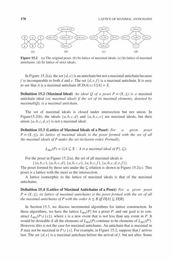
178 LATTICE OF MAXIMAL ANTICHAINS
d e f
{a,b,c,d,e,f}
{a,b,c,f} {a,b,c,d}
{a,b,c}
{a,b,c,e}
{d,e,f} {a,b,c}
{b,c} {a,b}
{ }
{a,c}{a,f} {c,d} {b,e}
{a,b,c}a b
(a) (b) (c) (d)
c
Figure 15.2 (a) The original poset. (b) Its lattice of maximal ideals. (c) Its lattice of maximalantichains. (d) Its lattice of strict ideals.
In Figure 15.2(a), the set {d, e} is an antichain but not a maximal antichain becausef is incomparable to both d and e. The set {d, e, f } is a maximal antichain. It is easyto see that A is a maximal antichain iff D(A) ∪ U[A] = X.
Definition 15.2 (Maximal Ideal) An ideal Q of a poset P = (X,≤) is a maximalantichain ideal (or, maximal ideal) if the set of its maximal elements, denoted bymaximal(Q), is a maximal antichain.
The set of maximal ideals is closed under intersection but not union. InFigure15.2(b), the ideals {a, b, c, d} and {a, b, c, e} are maximal ideals, but theirunion {a, b, c, d, e} is not a maximal ideal.
Definition 15.3 (Lattice of Maximal Ideals of a Poset) For a given posetP = (X,≤), its lattice of maximal ideals is the poset formed with the set of allthe maximal ideals of P under the set inclusion order. Formally,
LMA(P) = ({A ⊆ X ∶ A is a maximal ideal of P}, ⊆).
For the poset in Figure 15.2(a), the set of all maximal ideals is{{a, b, c}, {a, b, c, d}, {a, b, c, e}, {a, b, c, f }, {a, b, c, d, e, f }}.
The poset formed by these sets under the ⊆ relation is shown in Figure 15.2(c). Thisposet is a lattice with the meet as the intersection.
A lattice isomorphic to the lattice of maximal ideals is that of the maximalantichains.
Definition 15.4 (Lattice of Maximal Antichains of a Poset) For a given posetP = (X,≤), its lattice of maximal antichains is the poset formed with the set of allthe maximal antichains of P with the order A ⪯ B iff D[A] ⊆ D[B].
In Section 15.3, we discuss incremental algorithms for lattice construction. Inthese algorithms, we have the lattice LMA(P) for a poset P, and our goal is to con-struct LMA(P ∪ {x}), where x is a new event that is not less than any event in P. Itwould be desirable if all the elements of LMA(P) continue to be elements of LMA(P′).However, this is not the case for maximal antichains. An antichain that is maximal inP may not be maximal in P ∪ {x}. For example, in Figure 15.2, suppose that f arriveslast. The set {d, e} is a maximal antichain before the arrival of f , but not after. Some

AN INCREMENTAL ALGORITHM BASED ON UNION CLOSURE 179
algorithms explicitly determine the maximal antichains that get changed when a newevent arrives. In this chapter, the problem is circumvented by building the lattice ofstrict ideals instead of the lattice of maximal antichains. If S is a strict ideal of P, thenit continues to be one on arrival of x so long as x is a maximal element of P ∪ {x}.The lattice of strict ideals is isomorphic to the lattice of maximal antichains but easierto implement via an incremental algorithm.
Definition 15.5 (Strict Ideal) A set Y is a strict ideal of a posetP = (X,≤), if there exists an antichain A ⊆ X such that D(A) = Y.
Definition 15.6 (Lattice of Strict Ideals of a Poset) For a given poset P = (X,≤),its lattice of strict ideals is the poset formed with the set of all the strict ideals of Punder the set inclusion order.
Figure 15.2 shows a poset with the three isomorphic lattices: the lattice of max-imal ideals, the lattice of maximal antichains, and the lattice of strict ideals. To gofrom the lattice of maximal ideals to the lattice of maximal antichains, a maximalideal Q is mapped to the antichain maximal(Q). Conversely, a maximal antichain A ismapped to the maximal ideal D[A]. To go from the lattice of antichains to the latticeof strict ideals, a maximal antichain A is mapped to the set D(A). Conversely, a strictideal Z is mapped to an antichain as the minimal elements in Zc, the complement ofZ. For example, when Z equals {b, c}, its complement is {a, d, e, f }. The set of theminimal elements of the set {a, d, e, f } is {a, f }, which is the antichain correspond-ing to {b, c}. The correctness of this mapping is shown in the proof of correctness ofILMA algorithm (Theorem 15.7).
15.3 AN INCREMENTAL ALGORITHM BASED ON UNION CLOSURE
We now give an incremental algorithm to compute the lattice of maximal antichains.The ILMA algorithm is a modification of the algorithm given by Nourine and Ray-naud [NR99] based on computing the lattice of strict ideals.
The ILMA algorithm, shown in Figure 15.3, is based on computing closure underunion of strict ideals. It takes as input the poset P, an element x, and the lattice ofmaximal antichains of P. The poset and the lattice are assumed to be representedusing vector clocks. It outputs the lattice of maximal antichains of P′ = P ∪ {x}. Atstep 1, we compute the vector clock corresponding to the set D(x). The vector clockfor x, V corresponds to D[x]. By removing x from the set D[x], we get D(x). Theremoval of x is accomplished by decrementing S[i] in step 1. At step 2, we add S toL and make L closed under union.
The above-mentioned algorithm can also be used to compute the lattice of maximalantichains of any poset in an offline manner by repeatedly invoking the algorithmwith elements of the poset in any total order consistent with the poset. To start thealgorithm, the initial poset P would be a minimal element of P and the correspondinglattice L would be a singleton element corresponding to the empty strict downset.
We now show the correctness of the algorithm.

180 LATTICE OF MAXIMAL ANTICHAINS
Input: P: a finite poset as a list of vector clocksL: lattice of maximal antichains as a balanced binary tree of vectorclocksx: new element
Output: L′ ∶= Lattice of maximal antichains of P ∪ {x} initially L
//Step 1: Compute the set S ∶= D(x)Let V be the vector clock for x on process Pi;S ∶= V;S[i] ∶= S[i] − 1;
//Step 2: Add S and take closure with respect to unionif S ∉ L then
L′ ∶= L′ ∪ {S};forall vectors W ∈ L do
if max(W, S) ∉ L then L′ ∶= L′ ∪ max(W, S);
Figure 15.3 The algorithm ILMA for construction of lattice of maximal antichains.
Theorem 15.7 The lattice L′ constructed by ILMA algorithm is isomorphic to thelattice of maximal antichains of P′.
Proof: It is easy to verify that every vector in L′ is a strict ideal I of the posetP′ = P ∪ {x}. By induction, we can assume that L contains all the strict ideals ofP. Step (1) adds the strict ideal for D(x) and step (2) takes its union with all existingstrict ideals. Since max is an idempotent operation, it is sufficient to iterate over Lonce.
The bijection from L′ to the set of maximal antichains is as follows. Let I be astrict ideal in L′, i.e., there exists an antichain A such that D(A) = I. Let Ic denotethe complement of I, and let B equal to the set of the minimal elements of Ic.Thus, B = minimal(Ic). B is an antichain because it contains minimal elements of Ic.
It can be shown that B is a unique antichain for every strict ideal I. To showthat B is a maximal antichain, it is sufficient to show that D(B) ∪ U[B] = X.Since U[minimal(Ic)] = Ic, we get that U[B] = Ic by definition of B. We nowshow that D(B) ⊇ I from which our claim will follow because I ∪ Ic = X. SinceA ⊆ minimal(Ic), we get that A ⊆ B by definition of B. Since D(A) = I, we getD(B) ⊇ I. Hence, D(B) ∪ U[B] = X.
The time complexity of ILMA is dominated by step 2. Checking if the vector isin L requires O(𝑤 log m) time if L is kept as a balanced binary search tree of vectorclocks. Thus, the time complexity of step 2 is O(𝑤m log m). By repeatedly invokingILMA algorithm for a maximal element, we can construct DM completion of a posetwith n elements in O(n𝑤m log m) time. The space complexity is dominated by storage

AN INCREMENTAL ALGORITHM BASED ON BFS 181
requirements for L. With implicit representation, we have to store m elements whereeach element is stored as a vector of dimension𝑤 of coordinates each of size O(log n).Hence, the overall space complexity is O(m𝑤 log n).
15.4 AN INCREMENTAL ALGORITHM BASED ON BFS
In the ILMA algorithm, we traverse the lattice L for every element x. It requires us tomaintain the lattice L, which may be exponentially bigger than poset P, making thealgorithm impractical for large posets. We now show an online algorithm OLMA,which does not require the lattice L but only uses the poset P. Let M be the set ofnew elements (strict ideals) generated due to x. The time complexity of OLMA isdependent on the size of M independent of the size of the lattice L.
The incremental online algorithm OLMA is shown in Figure 15.4. At lines (1) and(2), we compute the vector S for the set D(x). At line (4), we check if S is already inLMA(P). Note that we do not store the lattice LMA(P). The check at line (4) is done bychecking if S is a strict ideal of P. If this is the case, we are done and M is an emptyset. Otherwise, we need to enumerate all strict ideals that are reachable from S in thelattice LMA(P′). We do so in lines (5)–(15) by traversing the strict ideals greater thanor equal to S in the BFS order. The set consists of strict ideals that have not beenexplored yet. At line (7), we remove the smallest strict ideal H and enumerate it atline (8). To find the set of strict ideals that are reachable by taking union with oneadditional event e, we explore the next event e after the ideal H along every process.There are two cases to consider.
If (D(e) ⊆ H), then the smallest event on process k that will generate newstrict ideal by taking union with H is the successor of e on process k, succ(e), ifit exists. Since D(succ(e)) contains e which is not in H, we are guaranteed thatmax(H,D(succ(e))) is strictly greater than H. It is also a strict ideal because itcorresponds to union of two strict ideals, H and D(succ(e)).
If (D(e) ⊈ H), then the smallest event on process k that will generate new strictideal by taking union with H is e. We add to the strict ideal max(H,D(e)).
It is left as an exercise to show that this method of BFS traversal is guaranteed toexplore all strict ideals greater than or equal to D(x) (see Exercise 1).
The function levelCompare in 15.4 provides a total order on all vectors. The vectorH deleted is the smallest in . Any vector that we add due to H is strictly greater thanH (either at line (11) or line (13)). Hence, once a vector has been deleted from , itcan never be added back again.
We now analyze the time and space complexity of the algorithm OLMA. Lines(7)–(15) are executed for every strict ideal in M. Suppose that the number of strictideals greater than or equal to D(x) is mx. The foreach loop at line (9) is executed 𝑤
times. Computing max of two vectors at lines (11) and (13) take O(𝑤) time. Adding itto the set takes O(𝑤 log𝑤L) time if is maintained as a balanced binary tree of thevectors, where 𝑤L is the maximum size of . Hence, the total time complexity forenumerating M is O(mx𝑤
2 log𝑤L). Recall that the ILMA algorithm traversed overthe entire lattice when adding a new element resulting in O(𝑤m log m) complexityfor incremental construction.

182 LATTICE OF MAXIMAL ANTICHAINS
Input: a finite poset P, x maximal element in P′ = P ∪ {x}Output: enumerate M such that LMA(P′) = LMA(P) ∪ M
(1) S := the vector clock for x on process Pi;(2) S[i] ∶= S[i] − 1;(3) if S is not a strict ideal of P then(4) // BFS(S): Do Breadth-First-Search traversal of M(5) := set of vectors initially {S};(6) while is nonempty do(7) H := delete the smallest vector from in the levelCompare
order;(8) enumerate H;(9) foreach process k with next event e do(10) if (D(e) ⊆ H) then(11) if succ(e) exists then ∶= ∪
{max(H,D(succ(e)))};(12) else(13) ∶= ∪ {max(H,D(e))};(14) endfor;(15) endwhile;(16) endif;
int levelCompare(VectorClock a, VectorClock b)(1) if (a.sum() > b.sum()) return 1; // a > b(2) else if (a.sum() < b.sum()) return -1; // a < b(3) for (int i = 0; i < a.size(); i++)(4) if (a[i] > b[i]) return 1;(5) if (a[i] < b[i]) return -1;(6) return 0; // a = b
Figure 15.4 The algorithm OLMA for construction of lattice of strict ideals.
We now compute the complexity of the OLMA algorithm to build the lattice forthe entire poset. For simplicity, we bound mx by m. Since the OLMA algorithm wouldbe called n times, the time complexity is O(nm𝑤2 log𝑤L).
The space complexity of the OLMA algorithm is O(𝑤L𝑤 log n) bits to store theset where 𝑤L is the maximum size that will take during BFS enumeration.
15.5 TRAVERSAL OF THE LATTICE OF MAXIMAL ANTICHAINS
In some applications (such as global predicate detection discussed in Section 15.6),we may not be interested in storing LMA but simply enumerating all its elements (orstoring only those elements that satisfy given property). Recall that the size of LMA(P)

TRAVERSAL OF THE LATTICE OF MAXIMAL ANTICHAINS 183
may be exponential in the size of the poset P in the worst case. In this section, weconsider the problem of enumerating all the maximal antichains of a computation inan offline manner. In the OLMA algorithm, we enumerated all strict ideals greaterthan or equal to D(x), when x arrives. We can use the OLMA algorithm in an offlinemanner as well. We simply use BFS({}) instead of BFS(D(x)) that enumerates all thestrict ideals. We call this algorithm BFS-MA.
We now show that the space complexity can be further reduced by using DFSenumeration of LMA. The DFS enumeration requires storage proportional to the heightof LMA, which is at most n.
In the previous section, we had used the lattice of strict ideals instead of latticeof maximal ideals. In this section, we use the lattice of maximal ideals because thelattice of maximal ideals is closed under intersection, which allows us to find thesmallest maximal ideal that contains a given set (at line (3) in 15.5).
One of the main difficulties is to ensure that we do not visit the same maximalantichain ideal twice because we do not store all the nodes of the lattice explicitly andhence cannot use the standard technique of marking a node visited during traversal.The solution we use is similar to that used for the lattice of ideals [AV01] and thelattice of normal cuts [Gar12]. Let pred(H) be the set of all maximal ideals that arecovered by H in the lattice. We use the total order levelOrder on the set pred(H). Wemake a recursive call on H from the maximal ideal G iff G is the biggest maximalideal in pred(K) in the total order given by levelOrder. To find pred(H), we first notethat every maximal antichain of a poset P is also a maximal antichain of its dual Pd.Hence, the lattice of maximal antichains of P is isomorphic to the lattice of maximalantichains of Pd. Traversing LMA(P) in the upward direction (in the Hasse diagram)is equivalent to traversing LMA(Pd) in the backward direction.
The algorithm for DFS enumeration is shown in Figure 15.5. From any maximalideal G, we explore all enabled events to find maximal ideals with at least oneadditional event. There are at most 𝑤 enabled events and for each event it takesO(𝑤2) time to compute the smallest maximal ideal K at line (3). At line (4), we checkif K covers G using the characterization provided by Reuter [Reu91] as follows.A maximal ideal K covers the maximal ideal G in the lattice of maximal ideals iff(K − G) ∪ (U[Maximal(G)] − U[Maximal(K)]) induces a complete height-onesubposet of P with (K − G) as the maximal elements and (U[Maximal(G)] −U[Maximal(K)]) as minimal element. This check can be performed in O(𝑤2) time.In line (5), we traverse K using recursive DFS call only if M equals G. Since therecan be 𝑤 predecessor for K and it takes O(𝑤2) time to compute each predecessor; thetotal time complexity to determine whether K can be inserted is O(𝑤3). ComputingM requires O(𝑤3) time. Hence, the overall time complexity of the algorithm isO(m𝑤4).
The main space requirement of the DFS algorithm is the stack used for recursion.Every time the recursion level is increases, the size of the maximal ideal increasesby at least 1. Hence, the maximum depth of the recursion is n. Therefore, the spacerequirement is O(n𝑤 log n) bits because we only need to store vectors of dimension𝑤 at each recursion level.

184 LATTICE OF MAXIMAL ANTICHAINS
Algorithm DFS-MaximalIdeals(G)Input: a finite poset P, starting state GOutput: DFS Enumeration of all maximal ideals of P
(1) enumerate(G);(2) foreach event e enabled in G do(3) K := smallest maximal ideal containing Q ∶= G ∪ {e};(4) if K does not cover G then go to the next event;(5) M := get-Max-predecessor(K) ;(6) if M = G then(7) DFS-MaximalIdeals(K);
function VectorClock get-Max-predecessor(K)//returns the predecessor that is the biggest in the levelCompare order
(1) H = maximal ideal in Pd that has the same maximal antichain as K(2) // find the maximal predecessor using maximal ideals in the dual poset(3) foreach event e enabled in the cut H in Pd do(4) temp := advance along event e in Pd from cut H;(5) // get the set of maximal ideals reachable in Pd
(6) pred(e) := smallest maximal ideal containing temp that covers H(7) return the biggest pred(e) in the levelCompare order;
Figure 15.5 Algorithm DFS-MA for DFS enumeration of lattice of maximal antichains.
15.6 APPLICATION: DETECTING ANTICHAIN-CONSISTENTPREDICATES
Global predicate detection problem has applications in distributed debugging, test-ing, and software fault-tolerance. The problem can be stated as follows. Given adistributed computation (either in an online manner or in an offline manner), anda global predicate B (a Boolean function on the lattice of consistent global states),determine if there exists a consistent global state that satisfies B. The global pred-icate detection problem is NP-complete [CG98] even for the restricted case whenthe predicate B is a singular 2CNF formula of local predicates [MG01a]. The keyproblem is that the lattice of consistent global states may be exponential in the sizeof the poset. Given the importance of the problem in software testing and monitor-ing of distributed systems, there is strong motivation to find classes of predicates forwhich the underlying space of consistent global states can be traversed efficiently. Inthis section, we describe an approach in which we construct the lattice of maximalantichains LMA instead of the lattice of consistent global states LI . The lattice LMA isusually much smaller (even exponentially smaller) than LI . We describe a class calledantichain predicate that satisfies the property that they hold on the lattice LI iff they
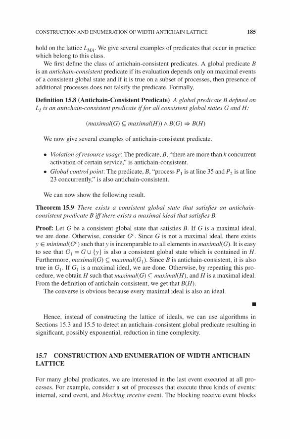
CONSTRUCTION AND ENUMERATION OF WIDTH ANTICHAIN LATTICE 185
hold on the lattice LMA. We give several examples of predicates that occur in practicewhich belong to this class.
We first define the class of antichain-consistent predicates. A global predicate Bis an antichain-consistent predicate if its evaluation depends only on maximal eventsof a consistent global state and if it is true on a subset of processes, then presence ofadditional processes does not falsify the predicate. Formally,
Definition 15.8 (Antichain-Consistent Predicate) A global predicate B defined onLI is an antichain-consistent predicate if for all consistent global states G and H:
(maximal(G) ⊆ maximal(H)) ∧ B(G) ⇒ B(H)
We now give several examples of antichain-consistent predicate.
• Violation of resource usage: The predicate, B, “there are more than k concurrentactivation of certain service,” is antichain-consistent.
• Global control point: The predicate, B, “process P1 is at line 35 and P2 is at line23 concurrently,” is also antichain-consistent.
We can now show the following result.
Theorem 15.9 There exists a consistent global state that satisfies an antichain-consistent predicate B iff there exists a maximal ideal that satisfies B.
Proof: Let G be a consistent global state that satisfies B. If G is a maximal ideal,we are done. Otherwise, consider Gc. Since G is not a maximal ideal, there existsy ∈ minimal(Gc) such that y is incomparable to all elements in maximal(G). It is easyto see that G1 = G ∪ {y} is also a consistent global state which is contained in H.Furthermore, maximal(G) ⊆ maximal(G1). Since B is antichain-consistent, it is alsotrue in G1. If G1 is a maximal ideal, we are done. Otherwise, by repeating this pro-cedure, we obtain H such that maximal(G) ⊆ maximal(H), and H is a maximal ideal.From the definition of antichain-consistent, we get that B(H).
The converse is obvious because every maximal ideal is also an ideal.
Hence, instead of constructing the lattice of ideals, we can use algorithms inSections 15.3 and 15.5 to detect an antichain-consistent global predicate resulting insignificant, possibly exponential, reduction in time complexity.
15.7 CONSTRUCTION AND ENUMERATION OF WIDTH ANTICHAINLATTICE
For many global predicates, we are interested in the last event executed at all pro-cesses. For example, consider a set of processes that execute three kinds of events:internal, send event, and blocking receive event. The blocking receive event blocks

186 LATTICE OF MAXIMAL ANTICHAINS
the process until it receives a message from some process. It is clear that if there areno in-transit messages and the last event executed at all processes is a receive event,then the system has a communication deadlock. In this example, we require that thelast event at each process be blocking receive. Even if one process is left out, thatprocess could send messages to all other processes unblocking them. This examplemotivates the following definition.
Definition 15.10 (Width Antichain) An antichain A is a width antichain of poset Pif its size is equal to the width of the poset.
Clearly, the set of all width antichains is contained in the set of all maximal antichains,which in turn is contained in the set of all antichains. It is left as an exercise to showthat the set of all width antichains (or maximum-sized antichains) form a distributivelattice [Dil50, Koh83], a sublattice of the lattice of all antichains.
On the basis of width antichains, we can define
Definition 15.11 (Width Ideal) An ideal Q of a poset P = (X,≤) is a width ideal ifmaximal(Q) is a width antichain.
Definition 15.12 (Width Predicate) A global predicate B defined on LI of adistributed computation on 𝑤 processes is a width predicate if B(G) ⇒|maximal(G)| = 𝑤.
We now give some examples of width predicate.
• Barrier synchronization: The predicate, B, “Every process has made a call tothe method barrier,” is a width predicate.
• Deadlock for dining philosophers: The predicate, B, “Every philosopher haspicked up a fork,” is also a width predicate.
Clearly, to detect a width antichain predicate, it is sufficient to construct or traversethe lattice of the width ideals. Here, we simply give the ideas behind the algorithm toconstruct or traverse the lattice.
Theorem 15.13 Given any finite poset P, there exists an algorithm to enumerate allits width antichains in O(𝑤2m) time where 𝑤 is the width of the poset P and m is thesize of the lattice of width antichains.
Proof:The width ideal lattice is a sublattice of the lattice of ideals with the same join
and meet operations. Since the lattice of ideals is distributive, so is the width ideallattice. Owing to its distributive property, this lattice is completely characterized byits join-irreducible elements. The join-irreducible elements of LWA(P) are given by
J(LWA(P)) = {the least width ideal that contains e | e ∈ P}
Given J(LWA(P)), the poset formed by the join-irreducibles, one can construct thedistributive lattice of all ideals by using algorithms to enumerate all ideals. There is

LEXICAL ENUMERATION OF CLOSED SETS 187
TABLE 15.4 Summary of Lattices Based on Antichains
Lattice Antichain Property Meet Join Distributive
Ideals All antichains Intersection Union YesMaximal Ideals Maximal Antichains Intersection Based on meet No
Width Ideals Antichains of size width Intersection Union Yes
1-1 correspondence between width ideals of P and ideals of J(LWA(P)). Hence, it issufficient to give an algorithm to construct J(LWA(P)). To this end, define a predicateB to be true on an ideal G iff maximal(G) forms a width antichain. The predicate Bis a regular predicate with an efficient advancement property, and therefore, we cancompute the slice (the set of all join-irreducibles) of P with respect to B in 𝑤2n timewhere n is the size of the poset P. Once we have the slice for B, we can enumerate allits ideals in𝑤2m time using the algorithms to enumerate ideals provided in Chapter 14where m is the number of width ideals of P (or, equivalently the number of ideals ofthe slice for B).
Table 15.4 gives a summary of the three lattices discussed in the chapter. Thelattice of ideals has 1-1 correspondence with the lattice of all antichains. Given anideal G, the set maximal(G) is an antichain. Given an antichain, A, D[A] is an ideal.In this lattice, the meet and join of two elements correspond to the intersection and theunion of ideals. The lattice of maximal ideals has 1-1 correspondence with the latticeof all maximal antichains. The meet in this lattice is the set intersection, but the join isnot union. It is defined based on the meets in the following standard manner: the joinof two maximal ideals G and H is the meet of all maximal ideals that contain bothG and H. The lattice of width ideals is in 1-1 correspondence with the antichains ofsize width. This lattice is a sublattice of the lattice of ideals with the meet and the joinoperations corresponding to the intersection and the union operations.
15.8 LEXICAL ENUMERATION OF CLOSED SETS
In this section, we give an algorithm to enumerate all the elements of the lattice ofmaximal antichains. The algorithm, due to Ganter and Reuter [GR91], is generalenough to enumerate any lattice that is a subset of the Boolean lattice (or a productspace) and is defined using a closure operator as defined in Chapter 6.
The algorithm in Figure 15.6 is a generalization of the algorithm to enumerate allideals in the lex order presented in Figure 14.5. At line (8), we compute H as theclosure of the set K. If H contains any new event from chains P1..Pk−1, we go to thenext iteration of the for loop; otherwise, H is the next lexically bigger closed set asshown by the following lemma.

188 LATTICE OF MAXIMAL ANTICHAINS
lexTraverseClosedSets(P)
Input: a poset POutput: All Closed sets in lex ordervar
G:array[1 …𝑤] of int initially ∀i ∶ G[i] = 0; // current closed setK:array[1 …𝑤] of int; // K = succ(G, k)H:array[1 …𝑤] of int; // H = closure(K)
(1) if G is closed enumerate(G);(2) while (G ≠ top) do // where top is the largest closed set(3) for k ∶= 𝑤 down to 1 do(4) if (there is no next event on Pk) continue;
// compute K ∶= succ(G, k)(5) K ∶= G;(6) K[k] ∶= K[k] + 1; // advance on Pk(7) for j ∶= k + 1 to 𝑤 do K[j] ∶= 0;
// compute closure(K); and determine if it is next in the lexorder
(8) H ∶= closure(K)(9) if (∃j ∶ 1 ≤ j ≤ k − 1 ∶ H[j] > G[j]) continue;(10) G ∶= H;(11) endfor(12) enumerate(G);(13) endwhile;
Figure 15.6 An algorithm for traversal of closed sets in lex order.
Theorem 15.14 The set H at line (10) is the next closed set in the lexical orderafter G.
Proof: H is a closed set because it is equal to closure(K). We only need to show thatit is the next closed set in the lexical order. Since K is lexically bigger than G, so isclosure(K). Hence, H is a closed set bigger than G. We only need to show that there isno closed set bigger than G and smaller than H. Suppose, if possible, there is anotherclosed set F bigger than G and smaller than H. Let f be the smallest index such thatF[f ] > G[f ]. If f < k, then we get that F > H because due to line (9), for all j smallerthan k, H[j] = G[j]. If f = k, then F is at least as big as K because K has K[j] equalto 0 for j > k. Hence, closure(F) ⊇ closure(K) = H. If f > k, then we would havetried F or a set smaller than F as K because at line (3), we try k in decreasing order.However, no index bigger than k was found.

LEXICAL ENUMERATION OF CLOSED SETS 189
TABLE 15.5 Definition of Closure Operators for Lattices
Lattice Closure (the condition for Y to be a closed set)
Ideals ideal(Y) ≡ (f ∈ Y) ∧ (e ≤ f ) ⇒ e ∈ YNormal cuts Yul = YMaximal ideals ideal(Y) ∧ (f ∉ Y ⇒ ∃e ∈ max(Y) ∶ e ≤ f )Maximum antichains ideal(Y) ∧ (|max(Y)| = 𝑤idth(P))
Assuming that the closure of the set can be done in O(𝑤2) time, we get the overallcomplexity of the algorithm as O(𝑤3C), where C is the number of closed sets.
Note that this algorithm allows us to enumerate all the following sets as shown inTable 15.5.
1. The set of all ideals: An ideal of a poset P = (X,≤) is a simply a subset of X thatis closed under ≤. A set Y ⊆ X is an ideal iff it satisfies the following condition:
(f ∈ Y) ∧ (e ≤ f ) ⇒ e ∈ Y .
However, for this case, we have already seen a more efficient algorithm inChapter 14 with time complexity O(𝑤2M) instead of O(𝑤3M) where M is thenumber of ideals and 𝑤 is the number of chains in P. There, we had to applyexactly one closure operator before getting the next lexically bigger closed set.
2. The set of all Normal cuts: A normal cut of P = (X,≤) is simply a subset Y ofX such that Yul = Y . It was shown in Chapter 6 that ul is a closure operator.
3. The set of all maximal ideals (or, the set of maximal antichains): The latticeof all maximal antichains is isomorphic to the lattice of all maximal ideals asshown earlier. An ideal Y for a poset (X,≤) is a maximal ideal iff it satisfies thefollowing condition:
f ∉ Y ⇒ ∃e ∈ max(Y) ∶ e ≤ f .
We leave it as an exercise to show that the definition satisfies properties forclosure.
4. The set of all width ideals (or, the antichains of size width). It is easy to showthat if G and H are width ideals, then so is G ∩ H. For any poset, P = (X,≤),if max(X) is a width ideal then, the set of all width ideals forms a toppedintersection-closed family. Hence, for any subset Y of X, there is a smallestideal, Z, such that its maximal elements form an antichain of size equal to thewidth of the poset. The set Z is closure of X. We leave this claim also as anexercise.

190 LATTICE OF MAXIMAL ANTICHAINS
TABLE 15.6 Generation of Lattices based on Unions
Lattice Basis Notation for Basis Elements
Ideals Principal ideals D[x] for all x ∈ XNormal Cuts Co-principal ideals X − D[x] for all x ∈ XMaximal Antichain Ideals Strict principal ideals D(x) for all x ∈ XWidth Ideals Least width-sized antichain ideals J(LWA(P))
15.9 CONSTRUCTION OF LATTICES BASED ON UNION CLOSURE
In this section, we show that all four lattices—the lattice of ideals, normal cuts,maximal ideals, and width ideals—can also be constructed using union closures. InFigure 15.3, we presented an algorithm to construct the lattice of maximum antichainideals based on union closure of strict principal ideals. Similar algorithms can bedesigned to construct the lattice of ideals, the lattice of normal cuts, and the lattice ofwidth ideals based on the union closure.
Table 15.6 shows the basis elements for union closure for various lattices corre-sponding to a poset (X ≤). The notation J(LWA(P)) corresponds to the join-irreducibleelements of the lattice of width antichains of P.
15.10 PROBLEMS
15.1. Show that the algorithm OLMA enumerates all strict ideals greater than orequal to D(x).
15.2. Give an algorithm for incremental construction of the lattice of maximalantichains based on DFS traversal.
15.3. Give parallel algorithms for online and offline construction of the lattice ofmaximal antichains.
15.4. Show that if G and H are maximal ideals, then so is G ∩ H.
15.5. Show that if G and H are width ideals, then so is G ∩ H.
15.6. Show that all four predicates on Y defined in Table 15.5 define closed familiesof subsets.
15.7. Give algorithms to compute closure of any set Y for all closure operatorsdefined in Table 15.5.
15.8. Show that the basis elements shown in Table 15.6 indeed generate the corre-sponding lattices.

BIBLIOGRAPHIC REMARKS 191
15.11 BIBLIOGRAPHIC REMARKS
Some earlier incremental algorithms for the lattice of maximal antichains are byJourdan, Rampon, and Jard [JRJ94] and Nourine and Raynaud [NR99, NR02]. Thediscussion of ILMA and OLMA algorithms is taken from [Gar13]. The discussionof lexical enumeration is taken from [GR91] and [Gar03]. Construction of latticesbased on union and intersection closure is also discussed in Nourine and Raynaud[NR99, NR02].
16DIMENSION THEORY
16.1 INTRODUCTION
The notion of dimension of a poset was introduced in a seminal paper by Dushnikand Miller [DM41]. The dimension of a poset, roughly speaking, is the dimension ofthe Euclidean space in which the poset can be embedded. The dimension of a posetreveals important information about the poset. For example, many problems that arealgorithmically hard for general posets, such as counting the number of ideals, areeasy for posets of dimension less than or equal to two. As we saw in Chapter 2, theconcept of dimension also lets us represent the order relation of a poset in an implicitmanner. The dimension theory of ordered sets has been an active area of research andthe reader will find a good survey of results in the book by Trotter[Tro92]. In thischapter, we cover only the most basic results and their applications.
We begin with the classical dimension theory based on notion of chain realizers.A chain realizer shows how a poset with n elements and dimension d can be repre-sented using d-dimensional vectors of coordinates from 0..n − 1. In Section 16.7, wediscuss string realizers that also use d coordinates but each coordinate may use fewerbits. Finally, in Section 16.8, we discuss rectangle realizers that always require lessor equal number of coordinates, with each coordinate requiring possibly fewer bitsthan required by the chain realizers.
Introduction to Lattice Theory with Computer Science Applications, First Edition. Vijay K. Garg.© 2015 John Wiley & Sons, Inc. Published 2015 by John Wiley & Sons, Inc.

194 DIMENSION THEORY
16.2 CHAIN REALIZERS
Theorem 2.1 in Chapter 2 shows that every poset has a linear extension. In dimensiontheory, we study if a poset can equivalently be represented using a small number ofits linear extensions. Let the operation of intersection of partial orders on the sameground set be defined as the intersection of the partial order relations. It is easy toverify that intersection of two partial orders is a partial order. Further, every finiteposet P is the intersection of all linear extensions of P. However, we may need onlya subset of these linear extensions to obtain P, which brings us to the following defi-nition.
Definition 16.1 (Realizer) A family R = {L1,L2,… ,Lt} of linear orders on X iscalled a realizer of a partial order P = (X,≤) if P = ∩Li∈RLi.
Definition 16.2 (Dimension) The dimension of P = (X,≤), denoted by dim(P), is thesize of the smallest realizer.
As a simple example consider the poset P defined on X = {a, b, c} with ≤ relationdefined as
≤= {(a, b), (a, c)}
The linear order L1 = {(a, b), (b, c), (a, c)} orders b less than c. The linear order L2 ={(a, c), (c, b), (a, b)} orders c less than b. It is easy to verify that when we take theintersection of L1 and L2, we get {(a, b), (a, c)}. Hence, {L1,L2} is a realizer of P.
For the poset P = (X,≤) shown in Figure 16.1, there are five linear extensions.The reader can verify that the intersection of these orders is exactly P. Clearly,dim(X,≤) ≥ 2 since it is not a chain. On the other hand, dim(X,≤) ≤ 2 sinceR = {L4,L5} is a realizer of P.
The reader should note the following facts. First, if x ≤ y, then x is less than y inall linear orders Li, because each of Li is a linear extension of P. If x||y in P, thenthe realizer of P must have at least one linear extension in which x is less than y andanother linear extension in which y is less than x.
c
c
c
c
ba
d
d c
d c
d
d
d
b
b
b
b ba a a
aa
L1 L2 L3 L4 L5
Figure 16.1 An example of a realizer.

STANDARD EXAMPLES OF DIMENSION THEORY 195
16.3 STANDARD EXAMPLES OF DIMENSION THEORY
The following family of examples is quite useful in studying dimension theory.For n ≥ 3, let Sn = (X,≤) be the height two poset with X = {a1, a2,… , an} ∪{b1, b2,… , bn}. The < relation is defined as follows. ∀ai, bj ∈ X, ai < bj in Sn iffi ≠ j. The poset Sn is called the standard example of an n-dimensional poset. Anexample is shown in Figure 16.2 for n equal to 5.
The standard example shows that the dimension of a poset can be large.
Theorem 16.3 (Dushnik-Miller [DM41]) dim(Sn) = n.
Proof:
• dim(Sn) ≤ n:For each i = 1, 2,… , n, define a linear order Li on X byLi = [a1, a2,… , ai−1, ai+1,… , an, bi, ai, b1, b2,… , bi−1, bi+1,… , bn]. Then R ={L1,L2,… ,Ln} is a realizer, so dim(Sn) ≤ n. Note that ai is less than bi in alllinear orders except Li.
• dim(Sn) ≥ n:Let R = {L1,L2,… ,Lt} be any realizer of Sn. Suppose, if possible, t < n. Sinceai||bi in P, there exists at least one linear order L in R in which bi is less thanai. We will say that L reverses the pair (ai, bi) if bi is less than ai in L. Sincethere are n pairs (ai, bi) and t linear orders where t < n, by pigeonhole principle,there exists at least one linear order Ls which reverses at least two pairs. Let thetwo pairs that it reverses be (ai, bi) and (aj, bj). Then bi < ai and bj < aj in Ls.However, aj < bi and ai < bj in P, so aj < bi and ai < bj in Ls. Thus, ai < bj <
aj < bi < ai in Ls which is clearly false. Therefore, t ≥ n. Hence, dim(Sn) ≥ n.
We now show the relationship between the dimension of a poset and the Euclideandimension. Let P = (X,≤P) and Q = (Y ,≤Q) be two posets. A map f from X to Y iscalled an embedding if for any x, x′ ∈ P
x ≤P x′ ≡ f (x) ≤Q f (x′).
b1 b2 b3 b4 b5
a1 a2 a3 a4 a5
Figure 16.2 Standard example S5.
196 DIMENSION THEORY
Clearly, if a poset P has dimension n, then there exists an embedding of P in n.Every element x ∈ P is mapped into a vector of dimension n such that the coordinatei of the vector equals the position of x in Li of a minimum realizer of P.
16.4 RELATIONSHIP BETWEEN THE DIMENSION AND THE WIDTHOF A POSET
In this section, we show that the dimension of a poset is always less than or equal tothe width of the poset. To prove this result, we first show a lemma due to Hiraguchi,which shows existence of a linear order with a special property for any given chain.
Lemma 16.4 (Hiraguchi [Hir55]) Let P = (X,≤) be a poset and let C ⊆ X be achain. Then, there exist linear extensions L1,L2 of P such that
1. y < x in L1 for every x, y ∈ X with x ∈ C and x||y in P.
2. y > x in L2 for every x, y ∈ X with x ∈ C and x||y in P.
Proof: We give a constructive proof of the first claim. The second claim is similar.We use induction on the size of C. When C is empty, the claim is vacuously true. Letz be the maximum element of the chain C. We partition the poset into two sets: U[z],the set of all elements that are greater than or equal to z and X − U[z]. In the subposet(X − U[z],≤), the size of C has decreased by one; hence, by induction, there existsa linear extension Ld such that for all x ∈ C − {z} and y ∈ X − U[z] such that x||y,y < x in Ld. Let Lu be any linear extension of the subposet (U[z],≤). We claim thatLd < Lu is a linear extension of P such that for any x ∈ C and y incomparable to x,y < x. The claim clearly holds for z because all incomparable elements to z appear inLd and z ∈ Lu. It also holds for all elements of C − {z} because if x ∈ C − {z} andy||x, then y ∈ X − U[z].
Let P = (X,≤) be a poset with A and B as any two subsets of X. If L is any linearorder of P, we say that A is over B, denoted by A∕B, if
∀a ∈ A, b ∈ B ∶ a||b ⇒ a > b in L
Thus, Hiraguchi’s lemma claims shows that there exists L1 that satisfies C∕X and L2that satisfies X∕C. Moreover, it is easy to convert the proof into an efficient algorithmfor constructing the linear order.
Theorem 16.5 (Dilworth [Dil50]) Let P = (X,≤) be a poset. Then dim(P) ≤𝑤idth(P).
Proof: We show this theorem by giving a realizer of size n = 𝑤idth(P). By Dilworth’schain partitioning theorem, there exists a partition X = C1 ∪ C2 ∪ · · · ∪ Cn, whereCi is a chain for i = 1, 2,… , n. We construct a realizer R = {L1,L2,… ,Ln} of P asfollows. For each Ci, we construct a linear extension Li of P such that Ci∕X in Li using
REMOVAL THEOREMS FOR DIMENSION 197
the procedure in Lemma 16.4. To show that R is a realizer of the poset, it suffices toshow that for every incomparable x and y in P, there exist a linear order in whichx < y. If y ∈ Ci, then Li gives us this property.
We later show a stronger result that dim(P) ≤ 𝑤idth(J(P)).A lower bound on the dim(P) can be provided using the width of the subposet ofdissectors of P. Let Dis(P) be the subposet formed by dissectors of a finite poset P.
Theorem 16.6 (Reading [Rea02]) Let P = (X,≤) be a poset. Then𝑤idth(Dis((P)) ≤dim(P).
We leave its proof as an exercise.
16.5 REMOVAL THEOREMS FOR DIMENSION
In this section, we show that the dimension of a poset does not decrease abruptlywhen a chain or an element is removed from the poset. The first theorem shows thatwhen a chain is removed, the dimension cannot decrease by more than 2.
Theorem 16.7 (Hiraguchi Chain Removal Theorem [Hir55]) Let P = (X,≤) bea poset and let C ⊊ X. Then
dim(X,≤) ≤ 2 + dim(X − C,≤).
Proof: Let Q be the poset after removal of the chain C. Let RQ be any realizer forQ of size t. We show that there exists a realizer of P of size t + 2. We first note thatany linear order L of Q can be extended to L′ such that L′ is a linear order of P(see Problem 3). We construct a realizer RP as follows. It contains t linear ordersof RQ extended for P and two additional linear orders that satisfy C∕X and X∕C,respectively. Given any pair of incomparable elements x, y ∈ X, we need to show thatthere exists a linear order in RP in which x < y. If both x and y belong to Q, thenone of the linear orders in RQ puts x before y. If x belongs to C, then the linear ordersatisfying X∕C satisfies x < y. If y belongs to C, then the linear order satisfying C∕Xsatisfies x < y.
The following theorem shows that when a point is removed from the poset, the dimen-sion cannot decrease by more than one.
Theorem 16.8 (Hiraguchi Point Removal Theorem [Hir55]) Let P = (X,≤) be aposet with |X| ≥ 2, and x ∈ X. Then
dim(X,≤) ≤ 1 + dim(X − {x},≤).

198 DIMENSION THEORY
Proof: Let Q be the poset after removal of the point x. Let RQ be the realizer of sizet for Q. Our goal is to construct a realizer of size t + 1 for P. We have to ensure thatfor every element y incomparable to x, there is one linear order that puts x below yand another one that puts y below x. For RP, we use first t − 1 linear orders from RQextended for P. From the last linear order of RQ, we construct two linear orders Luand Ld as follows. Let inc(x) be the set of elements incomparable to x. The linearorder Lu keeps x above inc(x) and Ld keeps x below inc(x). Lu is given by the orderLt(D(x) ∪ inc(x)) < x < Lt(U(x)), where the notation Lt(Z) represents the linear orderLt restricted to the set Z. Similarly, Ld is given by the order Lt(D(x)) < x < Lt(inc(x) ∪U(x)). To show that RP is indeed a realizer for P, it is sufficient to show that if a < bin Lt for incomparable a and b, then a < b either in Lu or Ld. If a < b in Lt but notin Lu, then a ∈ U(x). Similarly, If a < b in Lt but not in Ld, then b ∈ D(x). However,a ∈ U(x) and b ∈ D(x) implies that b < a in P, a contradiction.
The previous theorem allows us to remove any point in the poset withoutdecreasing the dimension by more than one. Can we remove two points from theposet such that the dimension does not decrease by more than one? It is clear thatwe cannot remove any two arbitrary elements (consider the standard example), butare there any two points that we can remove without decreasing the dimension bymore than one. This leads us to a famous open problem in dimension theory.
Conjecture: For all posets P = (X,≤) such that |X| ≥ 4, there exist x, y ∈ X :
dim(X,≤) ≤ 1 + dim(X − {x, y},≤).
Here is an example of a two-point removal theorem (under certain conditions).
Theorem 16.9 Let x and y be two distinct maximal elements of a poset P such thatD(x) ⊆ D(y). Then removal of x and y from P does not decrease the dimension bymore than one.
Proof: Let Q be the poset after removal of x and y. Let RQ be a realizer for Q. Weconstruct realizer for P as follows. For each linear order L in RQ, we have the linearorder L < y < x in RP. In addition, to RP, we add a linear order D(x) < x < D(y) −D(x) < y < (X − D(y) − {x, y}). It is easy to verify that RP is a realizer for P.
16.6 CRITICAL PAIRS IN THE POSET
We have seen that a crucial property of a realizer of a poset P is that for every incom-parable pair (x, y), there exists a linear order in the realizer that reverses the pair. Wenow introduce the notion of critical pairs which allows us to restrict our attention toa subset of incomparable pairs.

CRITICAL PAIRS IN THE POSET 199
b1 b2 b3
a1 a2 a3
Figure 16.3 Example of a critical pair: (a1, b1).
Definition 16.10 (Critical Pair) Let P = (X,≤) be a poset with incomparable ele-ments x and y. The ordered pair (x, y) is called a critical pair in P if:
1. D(x) ⊆ D(y), and
2. U(y) ⊆ U(x).
Observe that if x < y, the above-mentioned statements hold trivially. In Figure 16.3,while (a1, b1) is a critical pair, (b1, a1) is not. In Figure 16.1, (c, b) is a critical pair.
Theorem 16.11 (Rabinovitch and Rival [RR79]) Let P = (X,≤) be a poset and Rbe a family of linear extensions of P. Then, the following statements are equivalent.
1. R is a realizer of P.
2. For every critical pair (y, x), there is some L ∈ R for which x < y in L.
Proof: Let (y, x) be any incomparable pair. We show that there exists a linear orderin R that puts x < y. It is sufficient to show that there exists a critical pair (y′, x′)and that any linear order that reverses (y′, x′) also reverses (y, x). If (y, x) is a criticalpair, then we are done with y′ = y and x′ = x. Otherwise, either ¬(D(y) ⊆ D(x)) or¬(U(x) ⊆ U(y)). First, suppose ¬(D(y) ⊆ D(x)). This implies that there exists z, whichis in D(y) but not in D(x). Of all possible z, we choose a minimal element y′ in D(y)but not in D(x). The element y′ cannot be in U(x) because x and y are incomparable.Hence, x and y′ are incomparable. Furthermore, D(y′) ⊆ D(x) by minimality of y′ inD(y). Moreover, any linear order that puts x below y′ also puts x below y. If (y′, x) is acritical pair, we are done. Otherwise, from ¬(U(x) ⊆ U(y′)), we get that there exists amaximal x′ > x in P such that x′ and y are incomparable. It is easy to verify that (y′, x′)is a critical pair and any linear order that reverses (y′, x′) must have x ≤ x′ < y ≤ y′
and hence reverses (y, x).

200 DIMENSION THEORY
16.7 STRING REALIZERS
If a poset P with n elements has dimension d, then we can assign an implicit code toeach element x ∈ P such that the order relation between any two elements x, y ∈ Pcan be determined using their code. The code of any element x is a d-dimensionalvector 𝑣x where 𝑣x[i] equals the rank of x in the linear order Li of the realizer for P.By the definition of the realizer, we have that
x < y ≡ ∀i ∶ 𝑣x[i] < 𝑣y[i].
In this scheme, each element in x requires d log n bits. In this section, we look at analternative way of encoding posets that requires fewer bits.
As a motivating example, consider An, the poset on n elements that form anantichain of size n. Intuitively, this poset has no asymmetry and should require leastnumber of bits to encode. The binary relation corresponding to An is the emptyset. However, when we use a chain realizer for encoding this poset, we end upusing 2n log n bits for encoding the poset—2 log n bits for each element because thedimension of An is two. In the encoding scheme proposed in this section, we willuse just n bits to encode this poset. If we require that the code of any element be atleast one bit, this is clearly the best possible encoding for an antichain. We use a typeof poset called strings that are generalization of both chains and antichains as thebuilding block for realizers to reduce the number of bits required to encode a poset.We first give the definition of a string.
Definition 16.12 (string) A poset P = (X,≤) is a string if and only if ∃f ∶ X →
such that ∀x, y ∈ X ∶ x < y iff f (x) < f (y)The set of elements in a string which have the same f value is called a rank. Forexample, a poset (X,≤) where X = {a, b, c, d} and ≤= {(a, b), (a, c), (a, d), (b, d),(c, d)} is a string because we can assign f (a) = 0, f (b) = f (c) = 1, and f (d) = 2. Wecall f (x), the rank of element x. Here, b and c are in the same rank with rank equalto 1. The difference between a chain and a string is that a chain requires existenceof a one-to-one mapping such that x < y iff f (x) < f (y). For strings, we drop therequirement of the function to be one-to-one. We represent a finite string by thesequence of ranks in the string. Thus, P is equivalent to the string {(a), (b, c), (d)}.Note that in Chapter 13, we used the term ranking for these posets. We have used theterm string in this chapter to be consistent with the papers that analyzed this methodof encoding [GS01, RT10].
A chain is a string in which every rank is of size 1. An antichain is also a stringwith exactly one rank. Thus, a string generalizes both chains and antichains.
Observe that a string can be encoded very efficiently. Given the ranks of any twoelements, one can easily determine the order between them. Therefore, if all labels ofa string map to consecutive numbers, then the maximum number of bits required is⌈log2 r⌉, where r is the number of ranks in the poset. Note that this encoding drops thedistinction between elements that have the same order relationship with all other ele-ments. Thus, two elements x and y have the same code f (x) = f (y) iff for any elementz, (1) x < z iff y < z and (2) z < x iff z < y.

STRING REALIZERS 201
0 2 4
1 3 5
0
1
Figure 16.4 Encoding an infinite poset with strings.
a b
c d
b
a
d
c
Poset Chain Realizer
a
c
b
d
String Realizer
a
d
b d
b
c
c
a
L1 L2 s1 s2
Figure 16.5 A poset with a chain realizer and a string realizer.
This technique allows more efficient encoding of the partial order than the use ofchains as in dimension theory. At an extreme, the range of f may be finite even whenthe domain of f is infinite. For example, the order in Figure 16.4 where { all evennumbers } < { all odd numbers } on natural numbers can be encoded by assigning0 to all even numbers and 1 to all odd numbers. Such a poset cannot be assigned codesusing the classical dimension theory.
The following definition is useful in understanding the number of bits required toencode a poset.
Definition 16.13 Let P = (X,≤) be any poset. For x, y ∈ X, we say that x isorder-equivalent to y (denoted by x ∼ y) iff x is incomparable to y and for allz ∈ X ∶ x < z ≡ y < z and for all z ∈ X ∶ z < x ≡ z < y
We also say that two elements x and y have duplicate holdings if they areorder-equivalent. Let numeq(P) denote the number of equivalence classes of therelation ∼. It is clear that the number of bits required to encode a poset is at leastlog numeq(P). In the poset of Figure 16.4, there are only two equivalence classesand hence we were able to encode each class with a single bit.We write x ≤s y if x ≤ y in string s and x <s y if x < y in string s.
Definition 16.14 (String Realizer) For any poset P = (X,≤), a set of strings iscalled a string realizer iff ∀x, y ∈ X ∶ x < y in P if and only if
1. ∀s ∈ ∶ x ≤s y, and
2. ∃t ∈ ∶ x <t y.

202 DIMENSION THEORY
The definition of less-than relation between two elements in the poset based on thestrings is identical to the less-than relation as used in vector clocks. This is one ofthe motivation for defining string realizer in the above-mentioned manner. In a dis-tributed system where the code of elements is determined in a decentralized manner,the relationship between two events may not be known globally. Thus, if event e hap-pened before f , this relationship may be known only to a single process. From theperspective of other processes, e and f may be indistinguishable, for example, whenboth are internal to the process. This order is more easily captured where a vector u isdeemed as smaller than vector 𝑣 even when u is smaller than 𝑣 in just one componentand identical in all the other components.A string realizer for the poset in Figure 16.5 is given by two strings:
s1 = {(c), (d, a), (b)} s2 = {(d, b), (c, a)}
There are two important differences between definitions of string realizers and chainrealizers. First, if is a chain realizer of a poset P, then P is simply the intersection oflinear extensions in. This is not true for a string realizer (see Figure 16.5). Secondly,all the total orders in preserve P, i.e., x < y in P implies that x < y in all chains in. This is not true for string realizer. For example, d < a in poset P of Figure 16.5,but (d, a) appears as a rank in the string s1. We are only guaranteed that a will notappear lower than d in any string.Now, analogous to the dimension we define
Definition 16.15 (String Dimension) For any poset (X,≤), the string dimension of(X,≤), denoted by sdim(X,≤), is the size of the set with the least number of stringssuch that is a string realizer for (X,≤).
Example 16.16 Consider the standard example Sm. The following function f can beused to create a string realizer of Sm. For all k, i = 1, 2,… ,m,
fk(ai) ={
0 if k ≠ i1 otherwise
fk(bi) ={
0 if k = i1 otherwise
For example,a1 = (1, 0, 0,… , 0), b1 = (0, 1, 1,… , 1)a2 = (0, 1, 0,… , 0), b2 = (1, 0, 1,… , 1).
In this example, the length of each string is 2 and thus each element requires only mbits for encoding. If we use classical dimension based on total orders, each elementwould require m ∗ log m bits.

STRING REALIZERS 203
Example 16.17 Consider the poset (X,≤) as follows.X = {∅, {a}, {b}, {a, b}, {a, c}, {a, b, c}}P = {(A,B) ∈ X × X ∶ A ⊆ B}.
A string realizer for the poset can be obtained as follows. For each set A ∈ X, weuse a bit vector representation of the set A. Thus, {a, c} is represented by (1, 0, 1) andthe set {a, b} is represented by (1, 1, 0). This representation gives us a string realizerwith three strings such that every string has exactly two ranks. This example can beeasily generalized to get a string realizer of size n for any poset P that is a subposetof the Boolean lattice on n elements.
The following lemma is easy to show.
Lemma 16.18
1. Every set of strings on a set X defines a partial order.
2. A poset P is embeddable in k iff there is a string realizer of size k.
We now establish the relationship between string dimension and chain dimension. Itmay appear, at first, that the string dimension of a poset may be much smaller thanthe chain dimension. However, this is not the case as shown by the following result.
Theorem 16.19 (Equivalence Theorem) For any poset P = (X,≤) such thatsdim(P) ≥ 2,
sdim(P) = dim(P).
Proof: We first show that sdim(P) ≤ dim(P). It is sufficient to show that for any chainrealizer of size k, there exists a string realizer of equal or smaller size. Given a chainrealizer , we construct the string realizer as follows. Each chain is simply viewed asa string. Our obligation is to show that the order generated from the string realizer isthe same as the one based on chain realizer (recall that the definition of less than forstring realizer is different from less than in a chain realizer.) If x is less than y, then itappears below x in all chains; and therefore, in all strings. Hence, x is less than y inthe string realizer as well. If x and y are incomparable, then there is at least one chainthat puts x below y and another chain that puts y below x. The same holds for strings;and, therefore, x and y are incomparable in the string realizer as well.
We now show that dim(P) ≤ sdim(P), whenever sdim(P) ≥ 2.Given a string realizer of P, , we construct the corresponding chain realizer. We
achieve this by imposing an appropriate linear order on all nodes in the same rank ofthe string to form a chain.
First consider the case when a set of elements G belong to the same rank in allstrings. This means that all these elements are order-equivalent and incomparable toeach other. We will combine all these elements into one element say z. After findingthe chain realizer of the new set, we replace z with any total order on G in one of thechains and the dual of the total order in another chain. Observe that we can do thisbecause there are at least two chains due to our assumption of sdim(P) ≥ 2.

204 DIMENSION THEORY
b c
ed
a
e
d
c
b
a
d
e
b
a
c
b
a
d ec d e
ba
c
c f
b
a
f
a
c
b
(a) (b) (c) (d)
S1 S2 S1 S2
Figure 16.6 An example of converting a string realizer to a chain realizer.
Now assume that there are no two elements that are always in the same rank.Suppose that {x1, x2,… , xm} have the same rank r in any string s. For any pair ofelements, xi and xj, we have two cases. If whenever xi appears in different rank thanxj, it appears below xj, then we know that xi < xj. If in one string xi appears below xjand in another string it appears above xj, then xi is incomparable with xj. It is sufficientto do a topological sort of all elements in rank r since the topological sort preserves< order. By repeating this process for other ranks, we obtain a chain for the strings such that the resulting string realizer also realizes the same poset. We apply thisoperation to all strings to get a chain realizer.
Figure 16.6 shows an example of converting a string realizer into a chain realizer.Since d and e appear in the same rank in all strings, we first combine d and e into oneelement f . As a result, we get strings in Figure 16.6(c). We then untie the rank (c, f )by keeping c less than f in s1 and untie the rank (a, b) in s2 by keeping a less than b.We now have the chain order. Now we replace f by d and e, keeping d less than e ins1 and e less than d in s2 to get the chains in Figure 16.6(d).
The concept of string realizer has the advantage over chain realizer that it gener-ally requires less number of bits to encode a partial order by using strings than byusing chains. Using dimension theory, if a partial order has dimension k, then it canbe encoded using k ∗ log(n) bits. String realizers result in a lower number of bitsfor encoding. Let sbits(P) denote the minimum number of bits required to code anelement using a string realizer. Formally,
sbits(P) = min
∑
s∈⌈log(height(s))⌉,
where ranges over all string realizers of P. In other words, we consider all stringrealizers and use the one which results in the least number of bits.
The number of bits used by a string realizer is always less than or equal to thatused by a chain realizer, i.e.,

STRING REALIZERS 205
Theorem 16.20 For all posets P = (X,≤) with n elements and dimension k,
sbits(P) ≤ k log n.
Proof: From Theorem 16.19, sdim(P) ≤ dim(P) for all P. To encode a string of lengthl, we require ⌈log l⌉ bits. The length of each string is clearly less than or equal ton = |X|.
Note that for any nonstring poset, given a string realizer with k strings, there isalso a chain realizer with k chains. However, since chains are “longer” than strings ingeneral, it takes more bits to encode position in the chain. For the standard example,encoding using chain realizer takes n∕2 ∗ log n bits per element.
Another popular method to encode a partial order is to use “adjacency matrix”representation discussed in Chapter 2. Any partial order can be coded using log(n) + nbits per element using “adjacency matrix” type representation. For every element, westore a binary array of size n. Further, each element is assigned a unique index intothe array. Let index(x) be the index of x in 1..n and x.𝑣 be the n bit array for elementx. We set x.𝑣[index(y)] to 1 if x < y and to 0 otherwise. It is easy to determine therelationship between x and y given index(x), x.𝑣, index(y), and y.𝑣. We now show thatstring-based encoding is always better than adjacency matrix- based coding.
Theorem 16.21 For all posets P = (X,≤), we have
sbits(P) ≤ n.
Proof: We show a string realizer of n strings with each string of size 2. Let X ={x1, x2, ..., xn}. We construct a string si for each xi, 1 ≤ i ≤ n. Every string si has tworanks. The upper rank consists of xi and all elements greater than xi. The lower rankconsists of all elements smaller than xi and all elements that are incomparable to xi.
We now show that this is a proper string realizer of P. Consider any two elementsxi and xj. By symmetry, there are only two cases:
Case 1: xi < xjIn this case, xi is less than xj in string sj. In all other strings, xi appears either in thesame rank or in the lower rank as xj. Note that if xi appears in the upper rank forstring sk for any k, then xj also appears in the upper rank.
Case 2: xi||xjIn this case, xi is less than xj in string sj, but xj is less than xi in string si.
Note that we could have used a “dual” string realizer in the proof of Theorem 16.21in which each string si has two ranks as follows. The upper rank consists of all ele-ments bigger than xi and all elements that are incomparable to xi. The lower rank
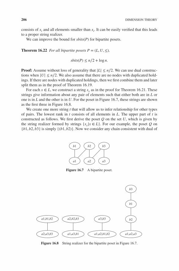
206 DIMENSION THEORY
consists of xi and all elements smaller than xi. It can be easily verified that this leadsto a proper string realizer.
We can improve the bound for sbits(P) for bipartite posets.
Theorem 16.22 For all bipartite posets P = (L,U,≤),
sbits(P) ≤ n∕2 + log n.
Proof: Assume without loss of generality that |L| ≤ n∕2. We can use dual construc-tions when |U| ≤ n∕2. We also assume that there are no nodes with duplicated hold-ings. If there are nodes with duplicated holdings, then we first combine them and latersplit them as in the proof of Theorem 16.19.
For each x ∈ L, we construct a string sx as in the proof for Theorem 16.21. Thesestrings give information about any pair of elements such that either both are in L orone is in L and the other is in U. For the poset in Figure 16.7, these strings are shownas the first three in Figure 16.8.
We create one more string t that will allow us to infer relationship for other typesof pairs. The lowest rank in t consists of all elements in L. The upper part of t isconstructed as follows. We first derive the poset Q on the set U, which is given bythe string realizer formed by strings {sx|x ∈ L}. For our example, the poset Q on{b1, b2, b3} is simply {(b1, b2)}. Now we consider any chain consistent with dual of
b1 b2 b3
a1 a2 a3
Figure 16.7 A bipartite poset.
a1,b1,b2 a2,b2,b3 a3,b3
a2,a3,b3 a1,a3,b1 a1,a2,b1,b2 a1,a2,a3
b2
b1
b3
Figure 16.8 String realizer for the bipartite poset in Figure 16.7.

STRING REALIZERS 207
the poset Q. For our example, a chain consistent with the dual of Q is b2 < b1 < b3.This string is the upper part of the string t and the lowest rank of t is all elements inL. The length of the string t is at most log n. For our example, t is the last string inFigure 16.8.
We show that this construction gives a string realizer for (L,U,≤). There are twocases.
Case 1: xi < xjThis case implies that xi ∈ L and xj ∈ U. By our construction, xi is less than xj instring t. xi appears in the upper rank in exactly one string si, but in that string xj isalso in the upper rank.
Case 2: xi||xjIf both xi and xj are in L, then we know that xi is less than xj in string sj and xj is lessthan xi in string si.
If both of them are in U, we have the following cases. If xi is less than xj in first|L| strings, then by our construction of t, it is greater than xj in string t. Otherwise,we know that in one of the strings among L strings xi is less than xj and in some otherstring xj is less than xi.
The last case is when xi is in L and xj is in U (or vice versa). In this case, xj is lessthan xi in string si and xi is less than xj in string t.
Our constructions of string realizers so far were dependent on the number of ele-ments. We now discuss a method that may result in a more efficient construction whenthe width of the poset is small.
Theorem 16.23 Every partial order P = (X,≤) on n ≥ 2 elements can be encodedusing a string realizer in at most log(height(P) + 1) ∗ 𝑤idth(P) bits.
Proof: For convenience, let 𝑤 = 𝑤idth(P). We use Dilworth’s chain coveringtheorem which states that (X,≤) can be partitioned into 𝑤 chains C1,C2, ...,C𝑤. Wethen use the transitively reduced diagram of (X,≤) with 𝑤 processes as given bythe chain decomposition. Further, we use Fidge and Mattern’s algorithm to assignvector timestamp for each event when the poset diagram is viewed as a computation.These vector timestamps determine a string realizer with 𝑤 coordinates such that nocoordinate is greater than height(P) + 1.
As an example, we show the encoding of the poset in Figure 16.7. Using this tech-nique, we use six bits to encode each element as the number of coordinates (width)is three and each coordinate requires two bits for encoding (Figure 16.9).
We can tighten the above-mentioned result by focusing on the subposet ofjoin-irreducibles of P. Let J(P) denote the subposet formed by the join-irreduciblesof P.

208 DIMENSION THEORY
b1:(2,0,0) b2:(1,2,0) b3:(0,1,2)
a1:(1,0,0) a2:(0,1,0) a3:(0,0,1)
Figure 16.9 Encoding for the bipartite poset in Figure 16.7.
b1:(2,0,0)
a1:(1,0,0) a2:(0,1,0) a3:(0,0,1)
b2:(1,1,0) b3:(0,1,1)
Figure 16.10 Another Encoding for the bipartite poset in Figure 16.7.
Theorem 16.24 Every partial order P = (X,≤) on n ≥ 2 elements can be encodedusing a string realizer in at most log(height(J(P)) + 1) ∗ 𝑤idth(J(P) bits.
Proof: For convenience, let𝑤 = 𝑤idth(J(P)) ≤ 𝑤idth(P). Let J(P) be partitioned into𝑤idth(J(P)) chains D1,D2, ...,D𝑤 chains. For every element x ∈ X, we assign thecode for x as follows. For each i ∈ {1..𝑤}, let
𝑣x[i] = |{z ∈ Di|z ≤ x}.|
It is easy to verify that x ≤ y iff 𝑣x ≤ 𝑣y. This code gives us the required string realizer.
Continuing with our example, we find that b2 and b3 are not join-irreducible.Hence, we get the code assignment as shown in Figure 16.10. We now use only 4bits to encode any element. The first coordinate requires 2 bits and the other twocoordinates require only 1 bit each.
We now define the notion of string length to derive a lower bound on dimensionof any poset. The length of a realizer for the poset P, denoted by slength(P,), isdefined as the length of the longest string in the string realizer of P. Let slength(P)denote the length of the longest string in the string realizer with the minimum numberof strings. The following lemma shows the relationship among dim(P), slength(P),and numeq(P).
Lemma 16.25 dim(P) ≥ log (numeq(P))∕ log (slength(P)).
Proof: The proof follows from the fact that the total number of codes is at mostslength(P)dim(P). Further, two elements in different equivalence classes cannot havethe identical code. This implies that slength(P)dim(P) ≥ numeq(P).

RECTANGLE REALIZERS 209
16.8 RECTANGLE REALIZERS
We have seen how we can represent a poset using chains and strings. Both methodsallowed us to encode elements of the posets with vectors of integers. We showedthat using vectors based on strings was more economical because we needed fewerbits to represent each coordinate in the vector. We now discuss an alternate approachin which our goal is to reduce the number of coordinates in the vector. In thisapproach, we use posets with dimension at most two—called two-dimensionalposets—as “building blocks” for realizing a given poset. For convenience, we referto two-dimensional posets as rectangles. An element x is less than another element yin the given partial order if and only if x is less than y in at least one of the rectangularorders and y is not less than x in any of the rectangular orders. The set of rectangularorders that realizes a given partial order constitutes its rectangular realizer. Inaddition, the rectangular dimension of a poset is the least number of rectangularorders needed to realize the corresponding partial order. Clearly, by definition, therectangular dimension of a poset is one if and only if its dimension is at most two.Trivially, the rectangular dimension of a poset is upper bounded by its dimension.
It turns out that there are posets with arbitrarily high dimension but only constantrectangular dimension. As an illustration, consider the family of standard examples.The dimension of 𝐒n is given by n for each n ≥ 3. This implies that O(n log n) bitsper element are required to encode 𝐒n using the dimension theory. We show in thissection that the rectangular dimension of 𝐒n is two for each n ≥ 3 and thus eachrectangle can be encoded using O(log n) bits. Therefore, using rectangles leads to amuch more efficient representation of 𝐒n.
We now formally define the notions of rectangle, rectangular realizer, and rectan-gular dimension of a poset.
Definition 16.26 (rectangle) A rectangle is a two-dimensional poset.
When a poset 𝐏 = (X,≤) is a rectangle, we call P as a rectangular order. For arectangular order R, we use R.1 and R.2 to refer to the two total orders that realizeR. In case the dimension of R is one, both R.1 and R.2 refer to the same total order.Clearly, R = R.1 ∩ R.2. A chain as well as an antichain is a rectangle.
Definition 16.27 (rectangular realizer) Let 𝐏 = (X,≤) be a poset. A family ={R1,R2, … ,Rt} of rectangular orders on X is called a realizer of P on X (also, realizes 𝐏) if for every x, y ∈ X, x < y in P if and only if y ≮ x in Ri for each i ∈ [1, t]and x < y in Rj for some j ∈ [1, t].
If x ‖ y in P, then in a rectangular realizer of P, two cases are possible. Eitherx ‖ y in all rectangular orders in or x < y in some rectangular order in and y < xin some other rectangular order in . On the other hand, if x < y in P, then x < y insome rectangular order in and x < y or x ‖ y in all other rectangular orders in .The notion of rectangular dimension can now be defined as follows:
Definition 16.28 (rectangular dimension) The rectangular dimension of aposet 𝐏 = (X,≤), denoted by rdim(X,≤) (or rdim(𝐏)), is the least positive integer t

210 DIMENSION THEORY
b1 b2 b3
a1 a2 a3
Figure 16.11 An example of a poset with rectangular dimension two.
for which there exists a family = {R1,R2,… ,Rt} of t rectangular orders on X sothat realizes 𝐏.
As an example, the rectangular dimension of the poset depicted in Figure 16.11is two. The two rectangular orders realizing it are given by {(a1 < a2 < a3 <
b1 < b2 < b3), (a3 < a2 < a1 < b3 < b2 < b1)} and {(b1 < a2 < b2 < a3 < b3 <
a1), (b3 < a1 < b2 < a3 < b1 < a2)}.We now show the result mentioned in the introduction.
Theorem 16.29 The rectangular dimension of 𝐒n is two for any n ≥ 3.
Proof: It is clear that the rectangular dimension of Sn is at least two because the chaindimension of Sn is n ≥ 3. We show a rectangular realizer with two rectangles. The firstrectangle, R1, encodes the complete bipartite poset in which all a’s are concurrent, allb’s are concurrent, and all a’s are less than all b’s. The second rectangle, R2, encodesn disjoint chains bi < ai for i = 1..n. It is easy to verify that {R1,R2} is a rectangularrealizer for Sn. Given any distinct ai, aj, they are concurrent in both the rectangles andtherefore ai ‖ aj in the realized poset. The same holds for bi and bj. Now consider aiand bj for i ≠ j. In R1, ai < bj and in R2, ai ‖ bj; therefore, ai < bj in the realized poset.Finally, ai < bi in R1 but bi < ai in R2; therefore, ai ‖ bi in the realized poset.
The rectangular dimension of a poset and its dual are identical because the dual ofa two-dimensional poset is again a two-dimensional poset.
The notions of rectangular realizer and rectangular dimension defined for a posetcan be generalized to any (acyclic) relation on a ground set. For a collection of rect-angular orders = {R1,R2,… ,Rt}, let rel() denote the relation realized by .For example, consider the rectangular orders {(a < b < c), (c < a < b)} and {(a <
b < c), (b < c < a)}. The relation realized by the two orders collectively is given by{(a, b), (b, c)}. Note that the relation is not transitive because it does not contain theordered pair (a, c).
16.9 ORDER DECOMPOSITION METHOD AND ITS APPLICATIONS
In this section, we give a method to construct rectangular realizers for a poset. In ourconstruction of rectangular realizers, we often use non-interfering rectangles.

ORDER DECOMPOSITION METHOD AND ITS APPLICATIONS 211
Definition 16.30 (non-interference) A rectangular order R is said to benon-interfering with a partial order P if R ⊆ P.
In addition, a rectangular realizer is non-interfering with a partial order if everyrectangular order in the realizer is non-interfering with the partial order. In otherwords, if two elements are incomparable in the partial order, they are also incom-parable in all rectangular orders in the realizer. In that case, the partial order is givenby the union of all rectangular orders in the realizer. Trivially, every partial order(even a relation) has a non-interfering rectangular realizer.
The main idea of the order decomposition method is as follows. Given a poset 𝐏 =(X,≤), we first decompose the partial order P into t suborders Pi for i = 1, 2,… , t. It isnot necessary for the suborders to be disjoint. We next compute a rectangular realizeri for each subposet (P,≤) such thati is non-interfering with P. Then, the collectionof rectangular orders = 1 ∪2 ∪ · · · ∪t constitutes a rectangular realizer of Pon X. When we specify a decomposition of a partial order into suborders, we do notenumerate the reflexive pairs which can always be added later.
Suppose the Hasse diagram (or covering graph) of a poset 𝐏 = (X,≤) is such thatevery element in the graph has at most one outgoing edge. In this case, the coveringgraph resembles a forest of trees. In particular, for every element x ∈ X, U(x) forms achain in P. Such a poset belongs to the class of series–parallel posets. The dimensionof a series–parallel poset is at most two and hence its rectangular dimension is at mostone. Similarly, a poset whose Hasse diagram is such that every element has at mostone incoming edge also has rectangular dimension of one.
A natural question to ask is what other posets have “small” rectangular dimension?In this section, we show that posets with “low” indegree have “small” rectangulardimension.
For a poset 𝐏 = (X,≤) and an element x ∈ X, let indegree of x in P be defined asthe number of elements less than x in P. The outdegree of an element can be duallydefined.
Theorem 16.31 Let 𝐏 = (X,≤) be a poset with the maximum value of in-degree forany node at most k where k ≥ 1. Then,
rdim(X,≤) ≤ k
Proof: The central idea is to decompose the partial order into at most k subor-ders such that the subposet induced by each suborder is a rectangle. For eachelement x ∈ X, number all elements in D(x) from 1 to |D(x)|. The ith subor-der Pi for i = 1, 2,… , k is given by the reflexive transitive closure of the set{(x, y) | x ∈ X and y is the ith element in D(x), if it exists}. Clearly, each elementhas at most one incoming edge in the Hasse diagram of (X,≤). Hence, (X,≤) is aseries–parallel poset, which implies that Pi is a rectangular order. Since Pi ⊆ P, Pi isnon-interfering with P. Therefore, it follows that the set {P1,P2,… ,Pk} constitutesa rectangular realizer of P on X.

212 DIMENSION THEORY
b3 b2 b1 b3 b2 b1
a3 a2 a1 a3 a2 a1
rectangle R1 rectangle R2
Figure 16.12 An example of decomposing a poset into series-parallel posets.
As an example of the construction in Theorem 16.31, consider the posetin Figure 16.11. The poset can be decomposed into two subposets shown inFigure 16.12 each with rectangular dimension one. The reader is referred to Mittaland Garg [MG04] for more details on the rectangular dimension.
16.10 PROBLEMS
16.1. Show that if P is a subposet of Q, then dim(P) ≤ dim(Q).
16.2. Show that all proper subposets of Sn have smaller dimension than n.
16.3. Let P = (X,≤) be a poset and Q be a subposet of P. Let L be a linear extensionof Q. Show that there exists a linear extension of P which restricted to Q isidentical to L. Give an efficient algorithm to construct such a linear extension.
16.4. Show that for every n, there exists an interval order with dimension greaterthan n.
16.5. Let C and D be two disjoint chains in P such that every element of chain Cis incomparable to every element in chain D. Show that removal of chains Cand D does not decrease the dimension by more than two.
16.6. ([Hir55] Let P = (X,≤) be a poset with |X| ≥ 4. Then
dim(X,≤) ≤|X|2
.
(Hint: Use Theorem 16.9 and Problem 5.)
16.7. Let J(P) be the subposet formed by the join-irreducibles and Dis(P) be thesubposet formed by dissectors of a finite poset P. Show that
𝑤idth(Dis(P)) ≤ dim(P).
(Hint: Show that P has the standard example of size equal to 𝑤idth(Dis(P))as a subposet.)

BIBLIOGRAPHIC REMARKS 213
16.8. [MG04] A subposet (Y ,≤) is called a critical subposet of the poset (X,≤) iffor every incomparable pair (x, y) from Y either (x, y) or (y, x) forms a criticalpair in the subposet (X ⧵ Y ,≤). Show that
rdim(X,≤) ≤ 1 + max {rdim(X ⧵ Y ,≤), dim(Y ,≤)}.
16.9. [MG04] Let P = (X,≤) = (L,U,≤) be a bipartite poset with nonempty L andU. Show that
rdim((X,≤)) ≤ min{⌈|L|∕2⌉, ⌈|U|∕2⌉}.
16.10. [MG04] Let P = (X,≤) be a poset such that for every element x ∈ X, eitherdegD(x) ≤ k or degD(x) ≥ |X| − k where k ≥ 1. Show that
rdim(X,≤) ≤ ⌈3k∕2⌉ + 1
16.11 BIBLIOGRAPHIC REMARKS
There is an excellent detailed treatment of dimension theory in the book by Trotter[Tro92]. The discussion of string realizer is from Garg and Skawratananond [GS01]and rectangular realizer is from Mittal and Garg [MG04].

17FIXED POINT THEORY
In this chapter, we introduce the notion of fixed points of a function defined overordered sets. The theory of fixed points allows us to obtain extremal solutions ofequations involving operations over lattices. For example, given any function f withsuitable properties, we can find x the least element in the lattice such that f (x) equals x.In computer science applications, we can use fixed point theory to define the meaningof recursion when functions are defined over lattices (or complete partial orders). Weillustrate these notions by defining probabilistic version of formal languages.
We begin by defining complete partial orders because they are weaker than com-plete lattices but still allow computation of fixed points. We then give Knaster–Tarskifixed point theorem that shows existence of least and greatest fixed points for mono-tone functions. If the function is continuous (a stronger property than monotonicity),then we show how one can give an explicit construction of the least fixed point.Section 17.3 gives applications of these results.
17.1 COMPLETE PARTIAL ORDERS
The completeness of a lattice is a strong property of posets and the given structuremay not always satisfy it. We consider a weaker requirement on a poset than that ofa complete lattice.
Introduction to Lattice Theory with Computer Science Applications, First Edition. Vijay K. Garg.© 2015 John Wiley & Sons, Inc. Published 2015 by John Wiley & Sons, Inc.

216 FIXED POINT THEORY
Definition 17.1 A poset (X,≤) is called a complete partial order (cpo) if
• inf X exists, and
• the least upper bound exists for any increasing chain of X.
Note that a complete lattice is always a cpo. The set of natural numbers with thenatural ordering is an example of a lattice which is not a cpo.
We are now ready to define properties of f . Recall that a function f is monotoneiff
∀x, y ∈ X ∶ x ≤ y ⇒ f (x) ≤ f (y)
A stronger property is continuity.
Definition 17.2 A function f ∶ X → X is called continuous or sup-continuous iff forall chains {xi},
f (⨆
i
xi) =⨆
i
f (xi)
It can be easily shown that every continuous operator is monotone.
17.2 KNASTER–TARSKI THEOREM
The following fixed point theorem is due to Knaster and Tarski [Tar55].
Theorem 17.3 Let L = (X,≤) be a complete lattice and f ∶ X → X be a monotonefunction on L. Then,(a) The least fixed point of f exists and is given by
z = inf {x | f (x) ≤ x}
(b) The greatest fixed point of f exists and is given by
z = sup {x | x ≤ f (x)}
Proof: We prove part (a) and leave part (b) as an exercise. For convenience defineZ = {x | f (x) ≤ x}. We first observe that since X is a complete lattice, the biggestelement ⊤ exists. Since f (⊤) ≤ ⊤, Z is nonempty. Completeness of X implies thatz = inf Z exists. Hence, z is well defined.We now show that f (z) ≤ z.
true⇒ { z is inf of Z }
∀y ∈ Z ∶ z ≤ y⇒ { f monotone }∀y ∈ Z ∶ f (z) ≤ f (y)
⇒ { f (y) ≤ y}∀y ∈ Z ∶ f (z) ≤ y
⇒ { z is the greatest lower bound}f (z) ≤ z

KNASTER–TARSKI THEOREM 217
We now show that z ≤ f (z)From above,
f (z) ≤ z⇒ { f monotone }
f (f (z)) ≤ f (z)⇒ { definition of Z}
f (z) ∈ Z⇒ { z is inf of Z }
z ≤ f (z)
We have shown that z is a fixed point. It is easy to see that it is the least fixed pointbecause all fixed points are also in Z.
It follows from Theorem 17.3 that a monotone function defined over a completelattice always has an infimal and a supremal fixed point. It lets us deduce the existenceof a fixed point but does not give us any method of computing it. The followingtheorem gives a method of computing fixed points under stronger conditions.
Theorem 17.4 Let f be a continuous function defined on a complete lattice. Let z =sup{f i(⊥)|0 ≤ i}. Then, z is the smallest fixed point.
Proof: We first show that z is a fixed point.
f (z)=
f (sup{f i(⊥)|0 ≤ i})= {f continuous}
sup{f i+1(⊥)|0 ≤ i}= {composition of f }
sup{f i(⊥)|1 ≤ i}= {⊥ is the smallest element}
sup{f i(⊥)|0 ≤ i}= { definition of z}
z
We now show that it is the smallest fixed point. Let y be any other fixed point. Since⊥ is the least element, ⊥ ≤ y. As f is monotone, we deduce that ∀i ∶ f i(⊥) ≤ f i(y).This means that ∀i ∶ f i(⊥) ≤ y as y is a fixed point. From this, we deduce that z ≤ yfrom the definition of z.
In the first part of Theorem 17.4, since {f i(inf X), i ≥ 0} is an increasing chain,f ∗(inf X) exists under the weaker condition that (X,≤) is a cpo. Thus it is possible tocompute the infimal fixed point of a sup-continuous function whenever it is definedover a cpo.

218 FIXED POINT THEORY
17.3 APPLICATION: DEFINING RECURSION USING FIXED POINTS
In this section, we show an application of fixed point theory to define probabilis-tic languages over a finite set of events. We also define operators under which theset of probabilistic languages (p-languages) is closed, thus forming an algebra ofp-languages. We show that this set is a complete partial order and our operators arecontinuous in it. Hence, recursive equations may be defined in this algebra using fixedpoints of continuous functions.
Definition 17.5 A p-language L over alphabet A is defined as L ∶ A∗ → [0, 1] withthe constraint that(C1) L(𝜖) = 1(C2) for all s ∶
∑a∈A L(sa) ≤ L(s)
The interpretation of L(s) is taken as the probability that s occurs in the system.(C1) says that the null string (𝜖) is always possible in the system. (C2) captures theproperty that if a system executes sa, then it must have executed s. Thus, the combinedprobability
∑a L(sa)must not be greater than L(s). (C2) also implies that if s is a prefix
of t, then L(s) is greater than or equal to L(t).On the basis of L, we can define a probability density function CL on the set A∗.
CL(s) = L(s) −∑
a
L(sa) for s ∈ A∗. (17.1)
The interpretation of CL(s) is that it is the probability that the system does s and stops,that is, it does not do anything afterward. We will drop the subscript L, when clearfrom the context. As
∑a L(sa) ≤ L(s), C(s) is always greater than or equal to zero.
Since L(s) is less than or equal to 1, so is C(s) for any s. Thus, C(s) always lies between0 and 1.
Example 17.6 Let L be defined as: L(𝜖) = 1,L(a) = 0.4,L(ab) = 0.2,L(b) =0.6,L(ac) = 0.1 and L(s) = 0 for all other strings s. Then, it is easy to see that Lsatisfies required properties. Hence, it is a p-language. Further, C for this p-languageis C(a) = 0.1,C(ab) = 0.2,C(ac) = 0.1,C(b) = 0.6.
Example 17.7 The nil language I is defined as I(𝜖) = 1, I(s) = 0 for s ≠ 𝜖. For thislanguage, CI(𝜖) = 1,CI(s) = 0 for s ≠ 𝜖.
Example 17.8 Consider a Bernoulli process. Every experiment has two outcomesa or b, with probability p and (1 − p), respectively. Here, our alphabet A = {a, b},and L(s) = p#(a,s)(1 − p)#(b,s) for any s ∈ A∗, where #(x, s) represents the number ofoccurrences of x in the string s. It is easy to check that this language satisfies (C1)and (C2). Also note that C(s) = 0 for any s.
We note that both p-languages and completion probability are functions definedfrom A∗ to [0, 1]. We call them language functions or simply functions. Let be the

APPLICATION: DEFINING RECURSION USING FIXED POINTS 219
set of all functions. We define a function Λ ∶ → as follows:
For any s, Λ(f )(s) =∑
a
f (sa)
Thus, if f is a p-language, then Λ(f ) gives the probability that the system will executesomething after s. It is easy to check that Λ is a linear functional. With this notation,the constraint (C2) on f is
Λ(f ) ≤ f .Similarly, for any p-language K, its corresponding completion probability densityfunction (pdf) is easily derived as
CK = K − Λ(K)
Now we make the following observations:
Lemma 17.9 (a)∑
s C(s) ≤ 1(b) For any s ∶ L(s) =
∑t C(st) iff limk→∞
∑|t|=k L(st) = 0
(c)∑
s C(s) = 1 iff limk→∞∑
|t|=k L(t) = 0
Proof: Proof (a) : We first show that∑
|s|=n L(s) ≤ 1. This can be shown using induc-tion on n. It is trivially true for n = 0. Assume that it is true for n = k. Then,
∑|s|=k+1 L(s)
= { s = ta }∑
|t|=k∑
a L(ta)≤ { (C2) }
∑|t|=k L(t)
≤{ Induction hypothesis }1
We now show that∑
s∈A∗ C(s) ≤ 1Let
S(n) =∑
|s|≤n
C(s)
Then∑
s C(s) = limn→∞ S(n) It is easy to show by induction that S(n) =1 −
∑|s|=n+1 L(s).
Therefore, 0 ≤ S(n) ≤ 1. Since {S(n)} is a monotone increasing sequence boundedabove by 1, the limit exists and is at most 1.
Proof (b): From equation (17.1), we get that
L(s) = C(s) +∑
a
L(sa)
Therefore, by repeated application of this equation, we get,L(s) =
∑|t|<k C(st) +
∑|t|=k L(st) for all k ≥ 1
= limk→∞∑
|t|<k C(st) + limk→∞∑
|t|=k L(st)=∑
t C(st) + limk→∞∑
|t|=k L(st)
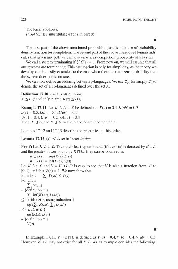
220 FIXED POINT THEORY
The lemma follows.Proof (c): By substituting 𝜖 for s in part (b).
The first part of the above-mentioned proposition justifies the use of probabilitydensity function for completion. The second part of the above-mentioned lemma indi-cates that given any pdf, we can also view it as completion probability of a system.
We call a system terminating if∑
C(s) = 1. From now on, we will assume that allour systems are terminating. This assumption is only for simplicity, as the theory wedevelop can be easily extended to the case when there is a nonzero probability thatthe system does not terminate.
We can now define an ordering between p-languages. We use (or simply ) todenote the set of all p-languages defined over the set A.
Definition 17.10 Let K,L ∈ . Then,K ⪯ L if and only if ∀s ∶ K(s) ≤ L(s)
Example 17.11 Let K,L,U ∈ be defined as : K(a) = 0.4,K(ab) = 0.3L(a) = 0.5,L(b) = 0.4,L(ab) = 0.3U(a) = 0.4,U(b) = 0.5,U(ab) = 0.4Then, K ⪯ L, and K ⪯ U, while L and U are incomparable.
Lemmas 17.12 and 17.13 describe the properties of this order.
Lemma 17.12 (,⪯) is an inf semi-lattice.
Proof: Let K,L ∈ . Then their least upper bound (if it exists) is denoted by K ⊔ L,and the greatest lower bound by K ⊓ L. They can be obtained as
K ⊔ L(s) = sup(K(s), L(s))K ⊓ L(s) = inf(K(s), L(s))
Let K,L ∈ and V = K ⊓ L. It is easy to see that V is also a function from A∗ to[0, 1], and that V(𝜖) = 1. We now show thatfor all s ∶
∑a V(sa) ≤ V(s).
For any s∑
a V(sa)= {definition ⊓ }
∑a inf(K(sa), L(sa))
≤ { arithmetic, using induction }inf (
∑a K(sa),
∑a L(sa))
≤ { K,L ∈ }inf (K(s), L(s))
= {definition ⊓ }V(s).
In Example 17.11, V = L ⊓ U is defined as V(a) = 0.4,V(b) = 0.4,V(ab) = 0.3.However, K ⊔ L may not exist for all K,L. As an example consider the following:

APPLICATION: DEFINING RECURSION USING FIXED POINTS 221
K(𝜖) = 1,K(a) = 0.6 L(𝜖) = 1,L(b) = 0.7 Then K ⊔ L is not defined (does not belongto ). Even though ⊔ may not exist for any set of p-languages, it exists for any chainof p-languages, i.e., a family of p-languages {Li | i = 0, 1..} such that Li ⪯ Li+1 forall i.
Lemma 17.13 ⪯ is a complete partial order(cpo) on the set . I is the least elementin this cpo.
Proof: It is easy to verify that ⪯ is reflexive, antisymmetric, and transitive. Thus, itis a partial order. We just need to show that if Li is a chain of p-languages, then itsleast upper bound exists. We define
⨆Li(s) = supi Li(s). This is well defined because
Li(s) is a monotonic sequence bounded above by 1. We also write it as limn→∞ Li(s).It is easy to see that
⨆Li is also a function from A∗ to [0, 1] and that
⨆Li(𝜖) = 1. We
now show thatfor all s ∶
∑a⨆
Li(sa) ≤⨆
Li(s).For any s,
∑a⨆
Li(sa)= {definition ⊔ }
∑a supi Li(sa))
= { Li monotone }∑
a limi→∞ Li(sa))= { finite sum }
limi→∞∑
a Li(sa))≤ { Li ∈ }
limi→∞ Li(s))= {definition
⨆}
⨆Li(s).
As a result of the above-mentioned lemma, we can easily compute fixed points ofcontinuous functions.
We now define some operations between various languages. These operators areuseful in describing a complex system as a combination of many simple systems.
The choice operator denoted by +e captures nondeterministic choice between twosystems. Given two p-languages L1 and L2, and a real number e between 0 and 1, thecombined system is denoted L1 +e L2 for e in [0, 1]. We use e to be equal to 1 − e.
Definition 17.14 L1 +e L2 = eL1 + eL2
The interpretation of the above-mentioned definition is: do L1 with probability eor L2 with probability 1 − e. It is easy to verify that the p-language defined earliersatisfies constraints (C1) and (C2). This operator can easily be generalized for mul-tiple arguments. In essence, the choice operator represents a convex combination ofp-languages.
We now derive an expression for the completion pdf for the composed system.C1 +e C2 = L1 +e L2 − Λ(L1 +e L2)= eL1 − Λ(eL1) + eL2 − Λ(eL2)= eC1 + eC2

222 FIXED POINT THEORY
The following proposition describes property of choice with respect to theordering.
Theorem 17.15 Choice is a continuous operator in both of its arguments.
Proof: We need to show that for any e,
K +e (⨆
i
Li) =⨆
i
(K +e Li)
This is easily verified using definitions.
The concatenation operator denoted by .e captures sequencing of two systems.Given two p-languages L1 and L2, and a real number e between 0 and 1, the combinedsystem is denoted by L1.eL2(s) for e in [0, 1]. Given any string t which is a prefix ofs, we use s∕t to denote the part of the string s left after removal of t.
Definition 17.16 L1.eL2(s) = L1(s) + e∑
t<s C1(t)L2(s∕t)= L1(s) − eC1(s) + e
∑t C1(t)L2(s∕t)
The above-mentioned definition has the following interpretation. The resulting sys-tem does L1 and then on completion does L2 with probability e. The probability thats occurs in the composed system is equal to the probability that it occurs in the firstsystem or a part of it occurs in the first system and a nonnull part in the second.It can be shown that is closed under the operation of .e. It is easy to check thatL1.eL2(𝜖) = L1(𝜖) − eC1(𝜖) + eC1(𝜖)L2(𝜖) = 1. Therefore, (C1) holds. We later derivean expression for C1.eC2 = L1.eL2 − Λ(L1.eL2) and show that it is always positive.Hence (C2) also holds.
We define the convolution operators between two real-valued functions on A∗ asfollows:
f ∘g(s) =∑
t
f (t)g(s∕t).
Thus, L1.eL2(s) is defined more simply as L1(s) − eC1(s) + eC1∘L2(s)The following proposition describes certain properties of the convolution operator.
Theorem 17.17 (a) Convolution is associative, i.e.,
f ∘(g∘h) = (f ∘g)∘h
(b) I is the identity for convolution, i.e.,
f ∘I = I∘f = f
(c) Convolution is continuous in both arguments, i.e.
f ∘(⨆
i
gi) =⨆
i
(f ∘gi), (⨆
i
fi)∘gi =⨆
i
(f ∘gi)

APPLICATION: DEFINING RECURSION USING FIXED POINTS 223
(d) Convolution is a linear operator, i.e.,
f ∘(𝛼g + h) = 𝛼f ∘g + f ∘h
(e) If g(𝜖) = 1Λ(f ∘g) = f ∘Λ(g) + Λ(f )
Proof: We leave (a) and (b) as an exercise. (c) We need to show that f ∘⨆
i gi =⨆i f ∘gi. For any s,
f ∘⨆
i gi(s)={definition ∘ }
∑t f (t)(
⨆i gi(s∕t))
= { real analysis }⨆
i∑
t f (t)gi(s∕t)={definition ∘ }
⨆i f ∘gi
The continuity in the other argument is similarly proved.
(d) For any s,f ∘(𝛼g + h)(s)=∑
t f (t)(𝛼g + h)(s∕t)=∑
t f (t)(𝛼g(s∕t) + h(s∕t))=∑
t f (t)𝛼g(s∕t) +∑
t f (t)h(s∕t))= 𝛼f ∘g + f ∘h
(e) For any s,Λ(f ∘g)=∑
a f ∘g(sa)=∑
a∑
t<=sa f (t)g(sa∕t)=∑
a∑
t≤s f (t)g(sa∕t) +∑
a f (sa)g(𝜖)= f ∘Λ(g) + Λ(f ).
We use f (2) to represent f ∘f . In general, we use f (i) to represent i times convo-lution of f with itself. This is well-defined because of associativity of ∘. We definef (0) to be the identity function, I. From the proof of associativity, we also note that∑
si,0≤i≤n−1 C(s0)C(s1)...C(sn−1) = C(n)(s). We show the following proposition.
Theorem 17.18 Let∑
s C(s) = 1. Then,∑
s C(n)(s) = 1 for all n.
Proof: We use induction on n. The proposition is clearly true for n = 1. Assume thatit is true for n = k. Then,
∑s C(k+1)(s)
=∑
s C(k)∘C(s)=∑
s∑
t C(k)(t)C(s∕t)=∑
u∑
t C(k)(t)C(u)=∑
u C(u)∑
t C(k)(t)= 1

224 FIXED POINT THEORY
We now derive the expression for completion probability for concatenation.C1.eC2 = L1.L2 − Λ(L1.L2)
= { definition of L1.L2}L1 + eC1 ∘ L2 − eC1 − Λ(L1 − eC1 + eC1 ∘ L2)
= {definition C1 = L1 − Λ(L1)}C1 + e(C1 ∘ L2 − C1 − Λ(C1 ∘ L2) + Λ(C1))
= { property convolution }C1 + e(C1 ∘ L2 − C1 − C1 ∘ Λ(L2))
= { property convolution, definition C2 }C1(s) + eC1 ∘ C2(s) − eC1(s)
= { definition e}eC1(s) + eC1 ∘ C2(s)We note that if e = 0, then the system is identical as before. On the other hand if
e = 1, then the resulting system is obtained as a pure convolution. Since convolutionis continuous, it is easy to show the following Theorem.
Theorem 17.19 Concatenation is continuous in its second argument, i.e.,
K.e
⨆
i
Li =⨆
i
K.eLi
Proof: K.e⨆
i Li= K − eC + eC ∘
⨆i Li
=⨆
i(K − eC + eC ∘ Li)=⨆
i K.eLi
However, concatenation is not even monotone in its first argument as shown bythe following example. Let K(a) = 0.2, and L(b) = 1.0. Now I ⪯ K, but I.1L is notcomparable to K.1L.
We are now ready to use fixed point theory to define recursion. For any K ∈ ,we can use +eK and .eK as unary operators defined from to itself. For any X ∈ ,+eK(X) = K +e X, and .eK(X) = K.eX. As shown earlier, both of these operators arecontinuous in the cpo of . Note that we use concatenation only in the second argu-ment as it is not continuous for the first argument. Therefore, any composition ofthese operators will also be continuous. We can define recursion operator denoted by𝜇X.F(x), where F is any function built out of the choice operator (+) and the concate-nation operator (.). We define 𝜇X.F(X) =
⨆Fi(I). From Theorem 17.4, we get that
⨆Fi(I) is the least fixed point of F. In other words, 𝜇X.F(X) satisfies the equation
X = F(X) and is the least such solution.
Theorem 17.20 Let {Xi} be a family of p-languages defined by Xn+1 = A + B.Xn,where + is simple pointwise addition in . Then, Xn = Bn.X0 +
∑i≤n−1 Bi.A
If . is replaced by ∘ uniformly, then the result holds.
Proof: Using induction on n.

APPLICATION: DEFINING RECURSION USING FIXED POINTS 225
Example 17.21 Let us consider the p-language defined by the following equation:X = K +e X. Then X =
⨆(K+e)i(I). We define Xn =
⨆i≤n(K+e)i(I). We list first few
Xn’s.X0 = IX1 = K +e IX2 = K +e (K +e I)Xj+1 = K +e XjXj+1 = eK + eXjThus, Xj = (eK)j +
∑i≤n−1 eieK (using Proposition 17.20). Then, X∗ = limj→∞ Xj.
We first consider the case when e = 1. Then, all Xj except X0 are K. Therefore,X∗ = K. When e = 0, then X∗ = I. When 0 < e < 1, the above-mentioned expres-sion in limit reduces toX∗ = (Σie
i)eK= (1∕(1 − e))eK= (1∕e)eK = K
Example 17.22 Consider the p-language defined by the following equation:X = K.eX. If e = 0, then X = K. We now assume that e > 0.Then X =
⨆(K.e)i(I). We define Xn =
⨆i≤n(K.e)i(I). We list first few Xn’s.
X0 = IX1 = K.eIX2 = K.e(K.eI)Xj+1 = K.eXjXj+1 = K − eC + eC ∘ XjWe use the following notation:
D(l, u) =i=u∑
i=l
eiC(i)
D(j) =∑
i≥j
eiC(i)
Thus, Xj = ejCj + D(0, j − 1) ∘ (K − eC)= ejCj + D(0, j − 1) ∘ K − D(1, j)= D(0, j − 1) ∘ K − D(1, j − 1)Thus, X∗ = D(0) ∘ K − D(1)
We will use this as the definition of repeated concatenation. This operator capturesrepetition of any system. Given any p-language L and a real number e between 0 and1, the combined system is denoted by L∗e (s) for e in [0, 1].
Definition 17.23 L∗e (s) =∑
n enC(n) ∘ L(s) −∑
i≥1 eiC(i)(s)= D(0) ∘ L − D(1)
The interpretation of the above-mentioned definition is— do L and then repeat it withprobability e.
Consider a process of tossing a coin which is repeated till the result of the toss isa head. Assuming that the tail comes with probability e, this system can be modeled

226 FIXED POINT THEORY
as follows:A = {toss}L(𝜖) = 1, L(toss) = 1, L(s) = 0 for other s.Then, our system is just repeated concatenation of L. For the primitive function,completion pdf is given by C(toss) = 1,C(s) = 0 for other s. By using formulas forconvolution, we obtain that C(k)(s) = 1 only for s = toss.toss.toss...k times. Thus,L∗e (tossk) = ek−1 + ek − ek = ek−1 for k ≥ 1 by Definition 17.23. This expressioncan be verified by calculating it directly from the problem.
17.4 PROBLEMS
17.1. Let (X,≤) be a complete lattice. A function f ∶ X → X is said to be disjunctiveif
∀Y ⊆ X ∶ f (⊔y∈YY) = ⊔y∈Y f (y);
it is said to be conjunctive if
∀Y ⊆ X ∶ f (⊓y∈YY) = ⊓y∈Y f (y);
it is said to be sup-continuous if
∀ increasing chain {yi, i ≥ 0} ⊆ X ∶ f (⊔i≥0yi) = ⊔i≥0f (yi);
it is said to be inf-continuous if
∀ decreasing chain {yi, i ≥ 0} ⊆ X ∶ f (⊓i≥0yi) = ⊓i≥0f (yi).
Prove that disjunctivity, conjunctivity, sup-continuity, and inf-continuity of feach imply monotonicity of f .
17.2. Consider the complete lattice (X,≤), where
X = {a, b, c, d}; ≤ = {(a, b), (a, c), (b, d), (c, d), (a, d)}.
Let f ∶ X → X be defined as f (a) = f (b) = f (c) = d and f (d) = d.
(a) Draw the Hasse diagram for the poset (X,≤).(b) Determine whether f is disjunctive or conjunctive.
17.3. Let (X,≤) be a complete lattice and f ∶ X → X be a function. f is said to beincreasing if x ≤ f (x),∀x ∈ X; it is said to be decreasing if f (x) ≤ x,∀x ∈ X.
(a) Prove that f ∗ is increasing and idempotent; and f∗ is decreasing, idempo-tent.
(b) If f is monotone (respectively, disjunctive), then show that f ∗ is monotone(respectively, disjunctive).
(c) If f is monotone (respectively, conjunctive), then show that f∗ is monotone(respectively, conjunctive).

BIBLIOGRAPHIC REMARKS 227
17.4. Let (X,≤) be a complete lattice and f ∶ X → X be a monotone function. Showthat the set of fixed points of f is also a complete lattice.
17.5. Let (X,≤) be a complete lattice and f ∶ X → X be a monotone function. Provethat sup{x ∈ X ∣ f (x) = x} = sup{x ∈ X ∣ x ≤ f (x)}.
17.6. Let (X,≤) be a complete lattice and f ∶ X → X be an inf-continuous function.Prove that f∗(sup X) is the supremal fixed point of f .
17.7. Show that the convolution operator defined on p-languages is associative withp-language I as its identity.
17.8. Compute the completion probability function for repeated concatenation, i.e.,compute C∗e = L∗e − Λ(L∗e ).
17.5 BIBLIOGRAPHIC REMARKS
One of the early results on existence of fixed points of a monotone function is dueto Knaster–Tarski [Tar55]. Lassez—Nguyen–Sonenberg [LNS82] provide a nice his-torical account of this and other fixed point theorems. The discussion of p-languagesis taken from Garg [Gar92].
INDEX
2-dimensional orders, 120
adversary, 48antichain, 4antisymmetric relation, 2asymmetric relation, 2
bipartite matching, 34Birkhoff’s Theorem, 101bottom element, 9
Catalan number, 128Catalan predicate, 111chain, 4closure operator, 63complete lattice, 7, 54, 61completion by cuts, 64computation, 12Connecting Lemma, 6cover relation, 3cross product of posets, 8crucial element, 111cut, 65
Dedekind–MacNeille completion, 64Dilworth’s Theorem, 29dimension, 23
Introduction to Lattice Theory with Computer Science Applications, First Edition. Vijay K. Garg.© 2015 John Wiley & Sons, Inc. Published 2015 by John Wiley & Sons, Inc.
disjoint sum, 8distributive, 92distributive lattice, 7down-set, 8dual poset, 74
efficient advancement property, 112equivalence, 3events, 11
Ferrer’s diagram, 13, 123Finitary Distributive Lattices, 104fixed point, 216function
conjunctive, 226disjunctive, 226inf-continuous, 226sup-continuous, 226
glb, 6graded poset, 97greatest lower bound, 6
Hall’s Theorem, 33happened-before, 11Hasse diagrams, 3height, 4
236 INDEX
incomparable, 4incremental algorithm for lattice completion, 69inf, 5inf semilattice, 6, 53infimum, 5integer partitions, 123interval order, 134inversions, 128irreflexive, 2irreflexive partial order, 3irreflexive transitive closure, 3
join, 5join-dense, 68join-irreducible, 10, 101join-preserving, 80join-prime, 100
kernel, 83Kleene closure, 63Knaster and Tarski, 216Konig–Egervary Theorem, 34
lattice, 6, 53lattice congruences, 82lattice homomorphism, 80lattice isomorphism, 80least upper bound, 6linear extension, 18linear predicate, 116linear sum, 8locally finite, 5lower cover, 4lower covering condition, 97lower dissector, 11lower-holdings, 9
matching, 34maximal, 10meet, 5meet-closed predicates, 110meet-dense, 68meet-irreducible, 10meet-preserving, 80merge, 42minimal, 10modular, 91, 100monotone, 80
nonseparating linear extensions, 143normal completion, 64normal ranking extension, 133
optimal chain decomposition, 50order filters, 9order ideals, 8, 107
p-diagram, 24partial order,complete, 216partition, 3Pentagon Theorem, 95, 100poset, 3principal filter, 64principal ideal, 64principal order filters, 9principal order ideals, 8
quadrilateral, 84quadrilateral-closed, 84queue insert graph, 44quotient lattice, 83
rank, 131ranked poset, 97ranking, 131ranking extension, 132realizer, 23recurrent vertices, 24reduced lattice, 83, 86reflexive, 2reflexive partial order, 3reflexive transitive closure, 3regular predicates, 113, 121relation, 2
Scott and Suppes’ Theorem, 134semiorder, 133series–parallel poset, 140set of distinct representatives, 33slice, 114strict partial order, 3strict split of a poset, 35sublattice, 54subposet, 4sup, 5sup semilattice, 6, 53sup-continuous, 216supremum, 5symmetric relation, 2
Topped ∩–structure, 63top element, 9topological sort, 18total order, 3transitive, 2
up-set, 9upper cover, 4upper covering condition, 97

INDEX 237
upper dissector, 11upper-holdings, 9
vector clock representation, 20vertex cover, 34
weak order, 131well-founded, 5width, 4
Young’s lattice, 13, 124