Introduction to XAFSGrant Bunker

Associate Professor, Physics

Illinois Institute of TechnologyRevised 4/11/97

Outline

Overview of Tutorial

1: Overview of XAFS

2: Basic Experimental design and methods

3: Basic Theory

4: Basic Data Analysis

5: Intermediate Experimental methods

6: Intermediate Theory

7: Intermediate Data Analysis

8: Summary and new developments

2 tutorial.nb

1: Overview of XAFS

What is XAFS?

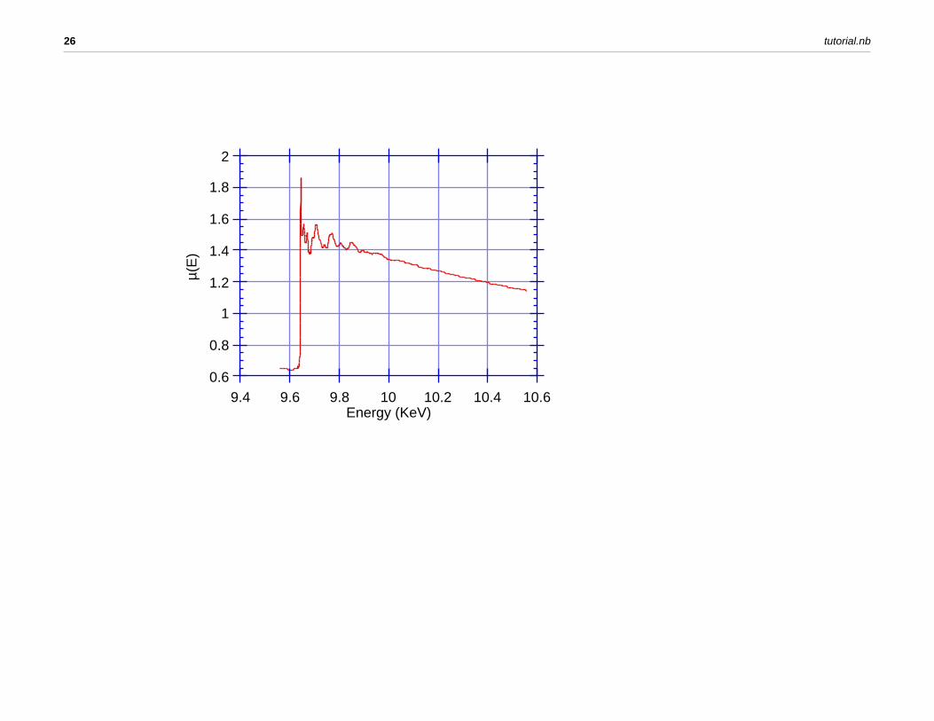
X-Ray Absorption Fine Structure (XAFS) refers to modulations in x-ray absorption coefficient around an x-ray absorption edge. XAFS is often divided (somewhat arbitrarily) into "EXAFS" (Extended X-ray Absorption Fine Structure) and "XANES" (X-ray Absorption Near Edge Structure).

The physical origin of EXAFS and XANES is basically the same, but several simplifying approximations are applicable in the EXAFS range, which permits a simpler quantitative analysis. XANES and EXAFS provide complementary information.

tutorial.nb 3

0.6

0.8

1

1.2

1.4

1.6

1.8

2

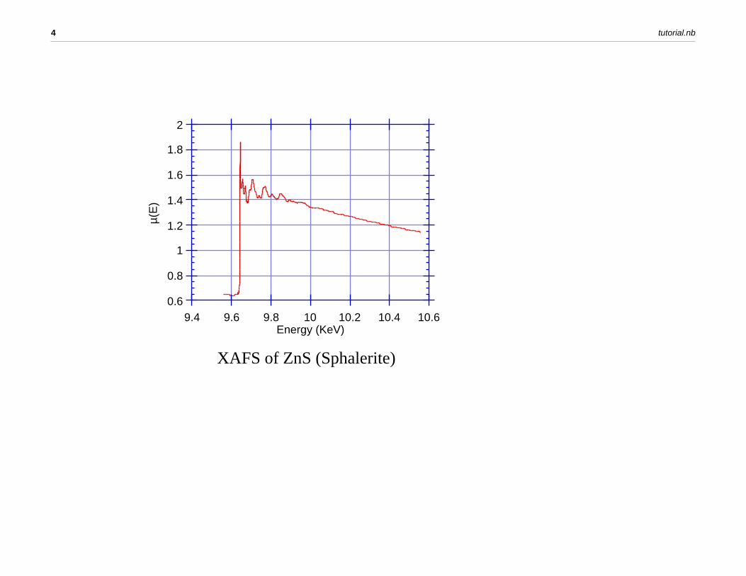
µ(E

)

9.4 9.6 9.8 10 10.2 10.4 10.6Energy (KeV)

XAFS of ZnS (Sphalerite)

4 tutorial.nb

A little history

XAFS was observed early in this Century by R. de L. Kronig. In molecular gases, Kronig, Petersson, Hartree, and others correctly explained the phenomenon in terms of electron multiple scattering. In condensed matter, however, interpretation of the data was much less clear. Various aspects of the phenomenon (e.g. accounting for thermal motion) were included over approximately a 50 year period, but as late as the 1960's it was unclear whether or not long range order was essential to explain the phenomenon.

Around 1970 a collaboration between Edward A. Stern, Dale Sayers, and Farrel Lytle cracked the problem and demonstrated how EXAFS could be used as a quantitative tool for structure determination.

The field has evolved significantly since 1970, and is advancing rapidly.

tutorial.nb 5

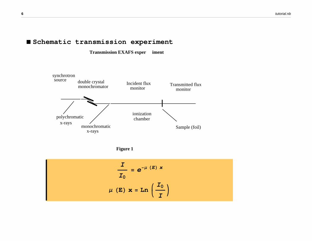
Schematic transmission experiment

Figure 1

Transmission EXAFS exper iment

synchrotronsource

monochromatordouble crystal

polychromaticx-rays

monochromaticx-rays

Incident flux monitor

ionizationchamber

Transmitted flux monitor

Sample (foil)

I

I0e E x

E x LnI0

I

6 tutorial.nb

0.6

0.8

1

1.2

1.4

1.6

1.8

2

µ(E

)

9.4 9.6 9.8 10 10.2 10.4 10.6Energy (KeV)

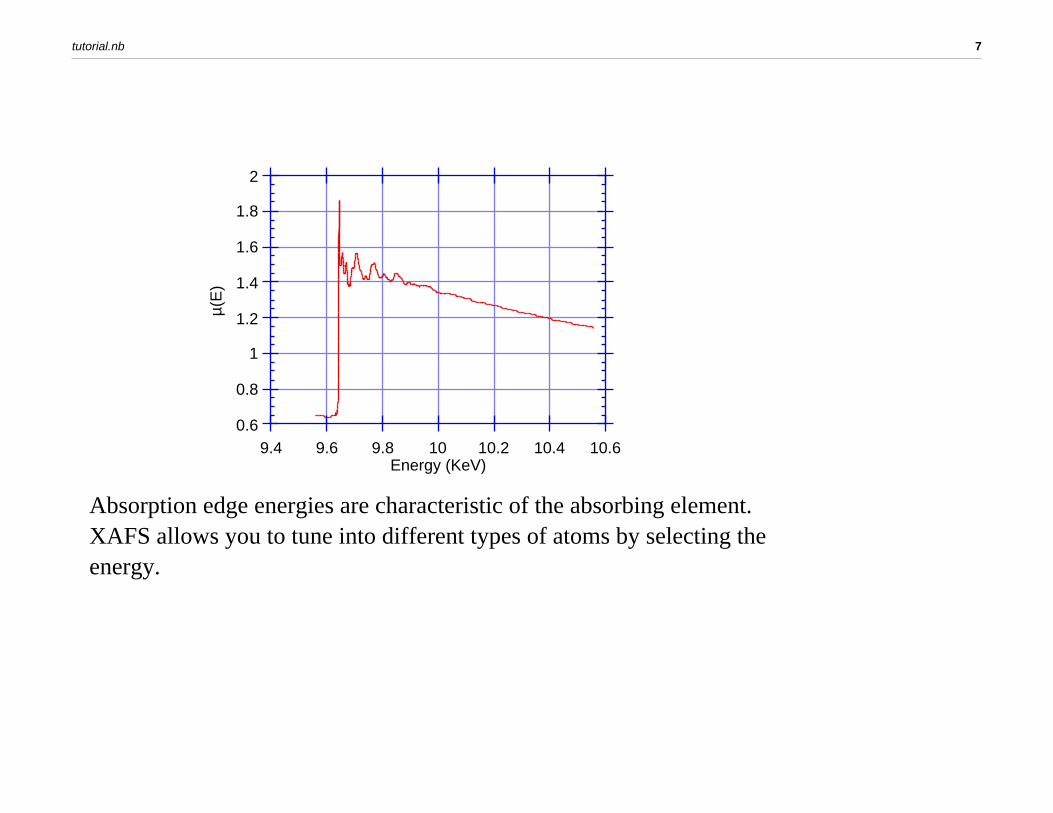
Absorption edge energies are characteristic of the absorbing element. XAFS allows you to tune into different types of atoms by selecting the energy.

tutorial.nb 7

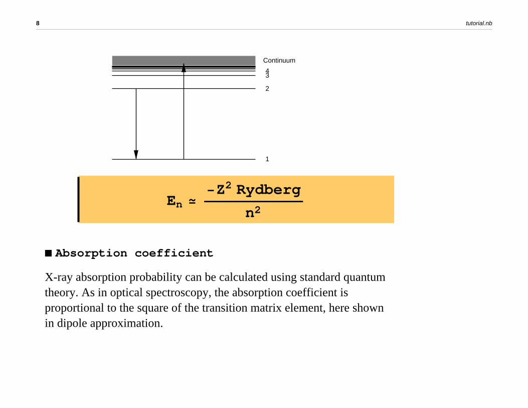
1

2

34

Continuum

EnZ2 Rydberg

n2

Absorption coefficient

X-ray absorption probability can be calculated using standard quantum theory. As in optical spectroscopy, the absorption coefficient is proportional to the square of the transition matrix element, here shown in dipole approximation.

8 tutorial.nb

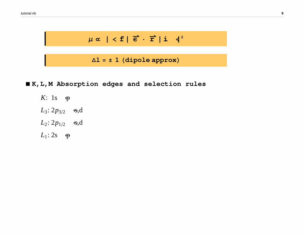
f r i 2

l 1 dipole approx

K,L,M Absorption edges and selection rules

K: 1s p

L3: 2p3 2 s,d

L2: 2p1 2 s,d

L1: 2s p

tutorial.nb 9

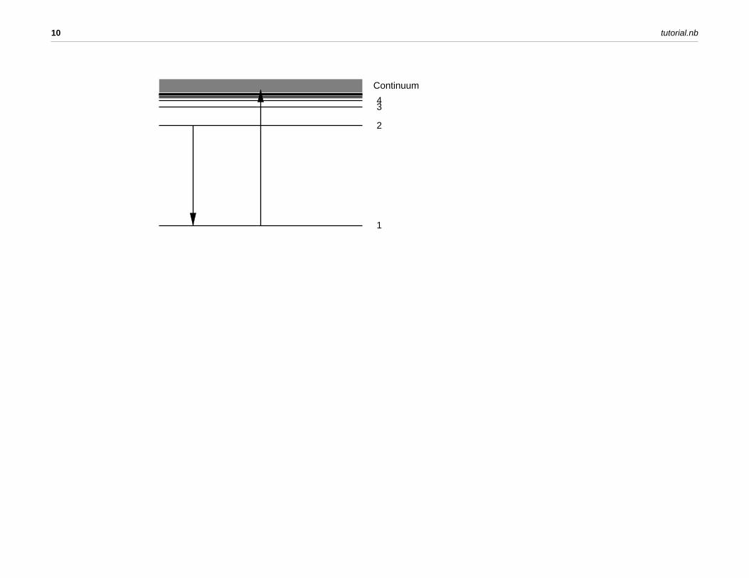
1

2

34

Continuum

10 tutorial.nb

0

200

400

600

800

1000

0 5 10 15 20 25 30 35 40

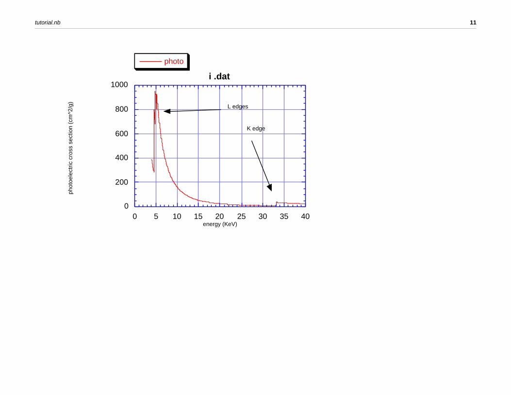
i .dat

photoph

otoe

lect

ric c

ross

sec

tion

(cm

^2/g

)

energy (KeV)

L edges

K edge

tutorial.nb 11

0

200

400

600

800

1000

2 4 6 8 10 12

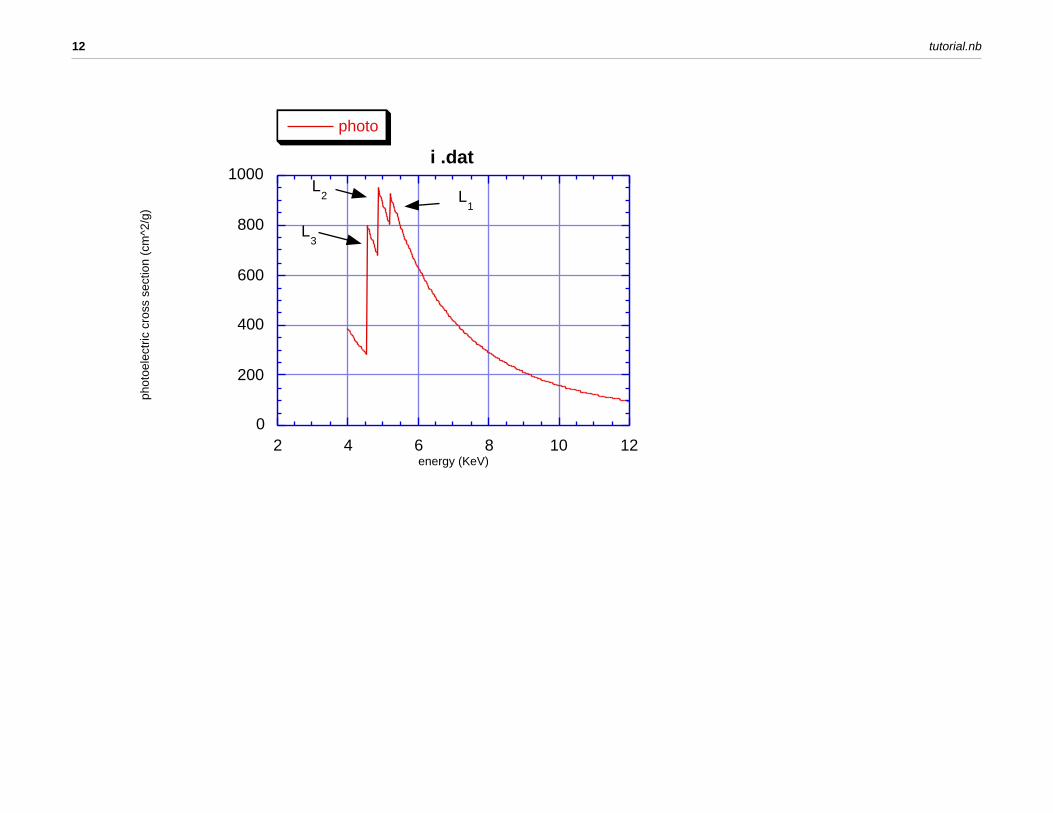
i .dat

photoph

otoe

lect

ric c

ross

sec

tion

(cm

^2/g

)

energy (KeV)

L3

L1

L2

12 tutorial.nb

-80

-60

-40

-20

0

20

40

60

80

32 33 34 35 36 37 38 39 40

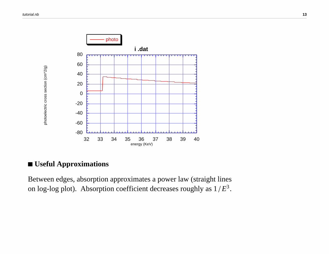
i .dat

photoph

otoe

lect

ric c

ross

sec

tion

(cm

^2/g

)

energy (KeV)

Useful Approximations

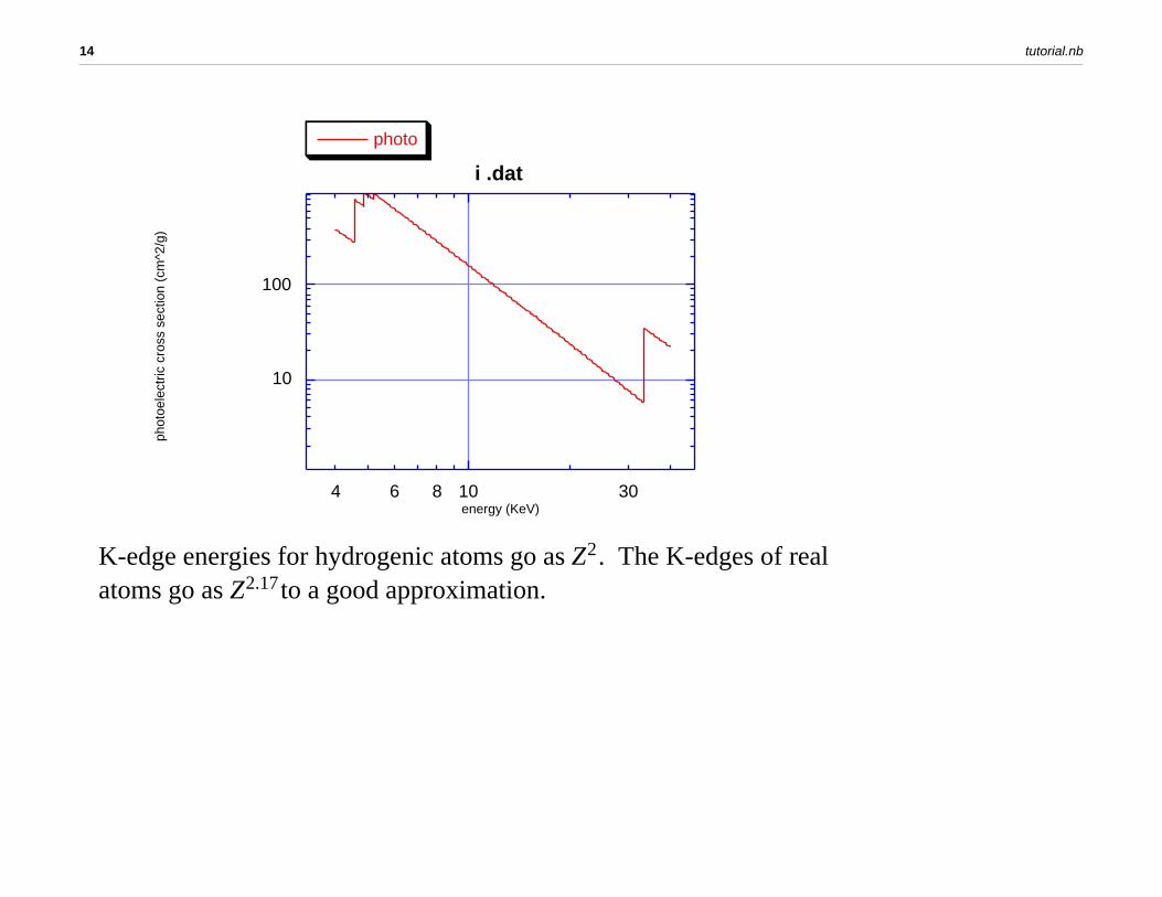
Between edges, absorption approximates a power law (straight lines on log-log plot). Absorption coefficient decreases roughly as 1 E3 .

tutorial.nb 13

10

100

4 6 8 10 30

i .dat

photoph

otoe

lect

ric c

ross

sec

tion

(cm

^2/g

)

energy (KeV)

K-edge energies for hydrogenic atoms go as Z2. The K-edges of real atoms go as Z2.17to a good approximation.

14 tutorial.nb

0

10

20

30

40

50

60

70

80

10 20 30 40 50 60 70 80

K

Z

E = c*Zp

c0.0059906p2.172R0.99997

0

10

20

30

40

50

60

70

80

10 20 30 40 50 60 70 80

edge energies (data)

K

tutorial.nb 15

1

10

100

10 100

edge energies (data)

K

K

Z

16 tutorial.nb

0

2

4

6

8

10

12

14

20 30 40 50 60 70 80

edge energies (data)

L1L2L3

L1

Z

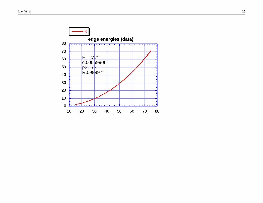
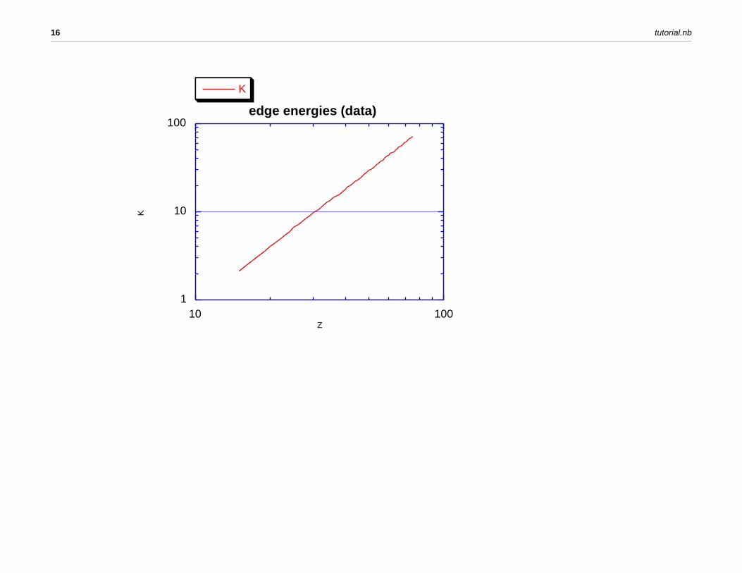
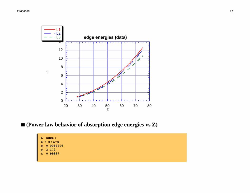
(Power law behavior of absorption edge energies vs Z)

K edge :E c Z^pc 0.0059906p 2.172R 0.99997

tutorial.nb 17

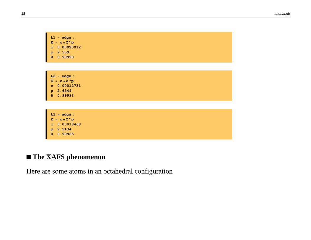
L1 edge :E c Z^pc 0.00020012p 2.559R 0.99998

L2 edge :E c Z^pc 0.00012731p 2.6549R 0.99993

L3 edge :E c Z^pc 0.00018468p 2.5434R 0.99965

The XAFS phenomenon

Here are some atoms in an octahedral configuration

18 tutorial.nb

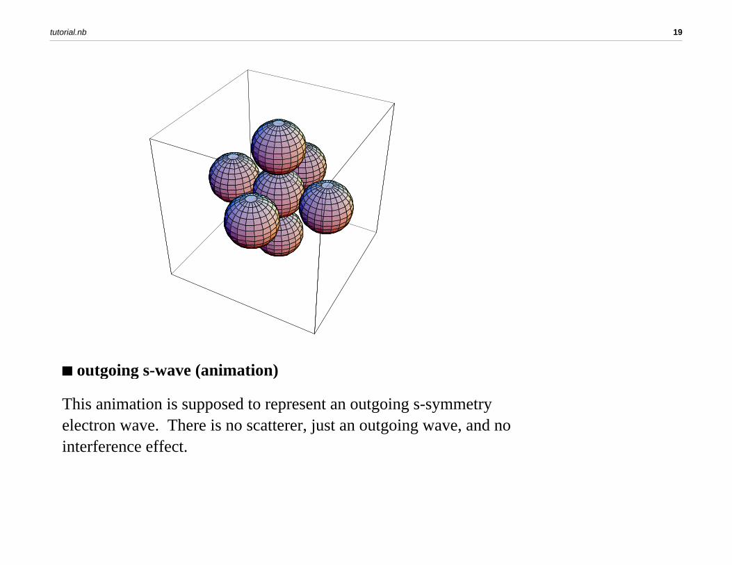
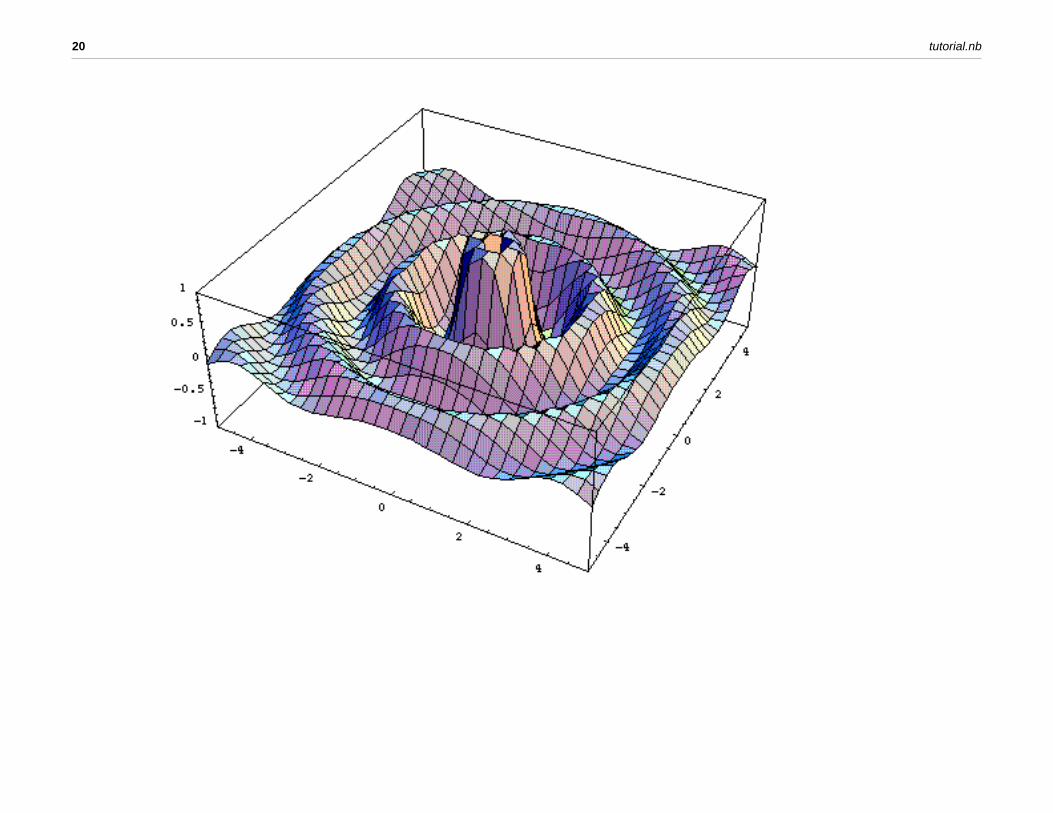
outgoing s-wave (animation)

This animation is supposed to represent an outgoing s-symmetry electron wave. There is no scatterer, just an outgoing wave, and no interference effect.

tutorial.nb 19

20 tutorial.nb

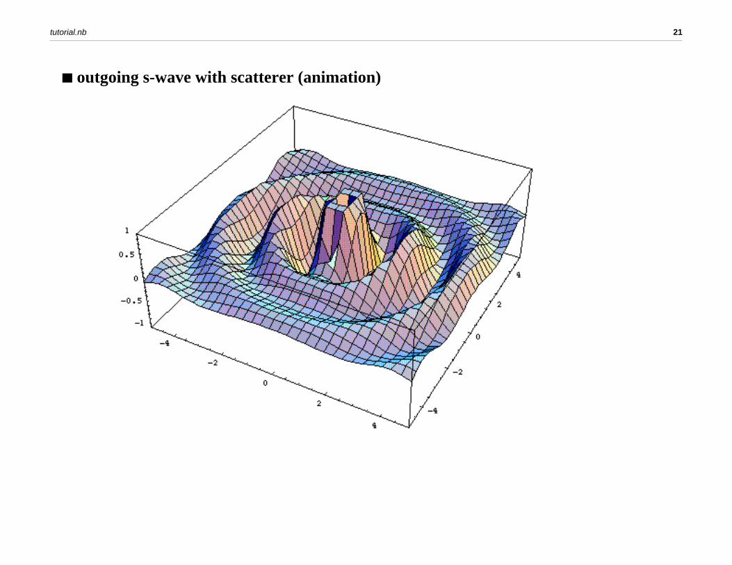
outgoing s-wave with scatterer (animation)

tutorial.nb 21

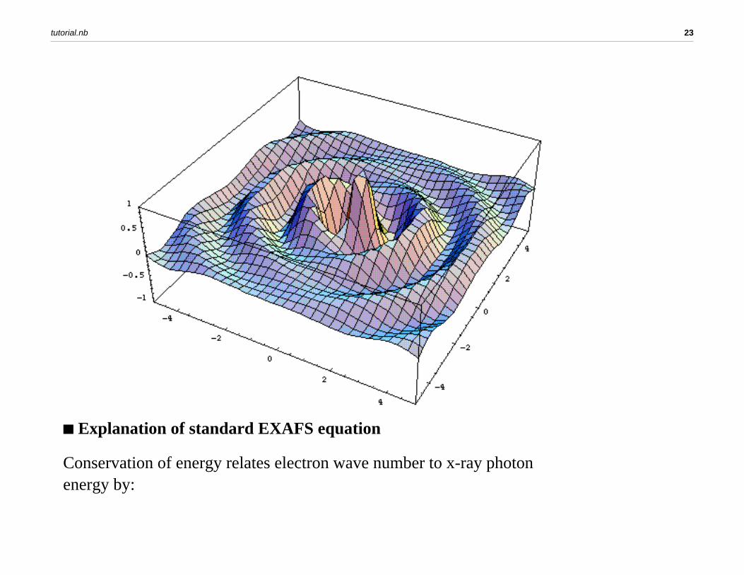
spherical p-wave (animation)

This animation is supposed to represent the outgoing p-symmetry electron wave. The wave amplitude is zero in the direction perpendicular to the x-ray electric polarization vector, which gives a Cosine squared angle dependence for oriented samples.

22 tutorial.nb

Explanation of standard EXAFS equation

Conservation of energy relates electron wave number to x-ray photon energy by:

tutorial.nb 23

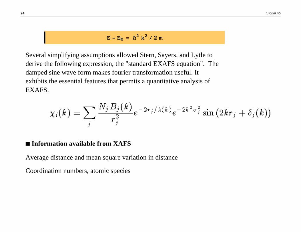
E E02 k2 2 m

Several simplifying assumptions allowed Stern, Sayers, and Lytle to derive the following expression, the "standard EXAFS equation". The damped sine wave form makes fourier transformation useful. It exhibits the essential features that permits a quantitative analysis of EXAFS.

Information available from XAFS

Average distance and mean square variation in distance

Coordination numbers, atomic species

24 tutorial.nb

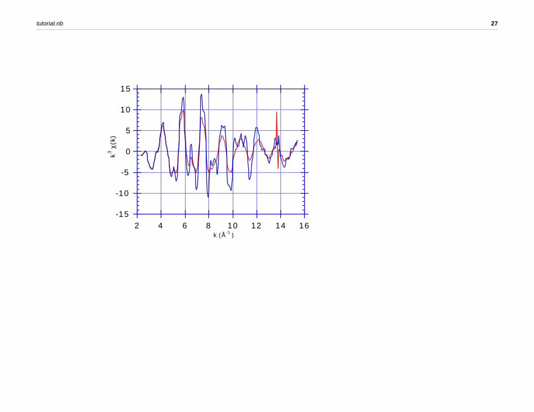
EXAFS data reduction and data analysis

Steps in traditional EXAFS data analysis:

1) correction for instrumental effects

2) normalization to unit edge step

3) interpolation to k-space

4) background subtraction

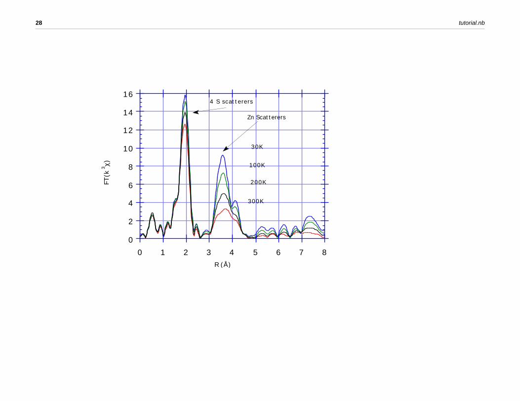
5) weighting, k-windowing, and fourier transform

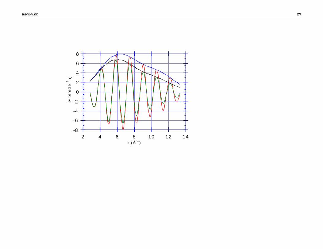
6) r-windowing and inverse transform to isolate single shell data

7) analysis of single shell amplitude and phase

tutorial.nb 25

0.6

0.8

1

1.2

1.4

1.6

1.8

2

µ(E

)

9.4 9.6 9.8 10 10.2 10.4 10.6Energy (KeV)

26 tutorial.nb

-15

-10

-5

0

5

10

15

2 4k (Å-1 )

6 8 10 12 14 16

k3 χ(k

)

tutorial.nb 27

0

2

4

6

8

10

12

14

16

0 1 2 3 4 5 6 7 8

FT(k

3 χ)

R (Å)

30K

100K

200K

300K

4 S scatterers

Zn Scatterers

28 tutorial.nb

-8

-6

-4

-2

0

2

4

6

8

Filt

ered

k3 χ

2 4 6 8 10 12 14k (Å-1)

tutorial.nb 29

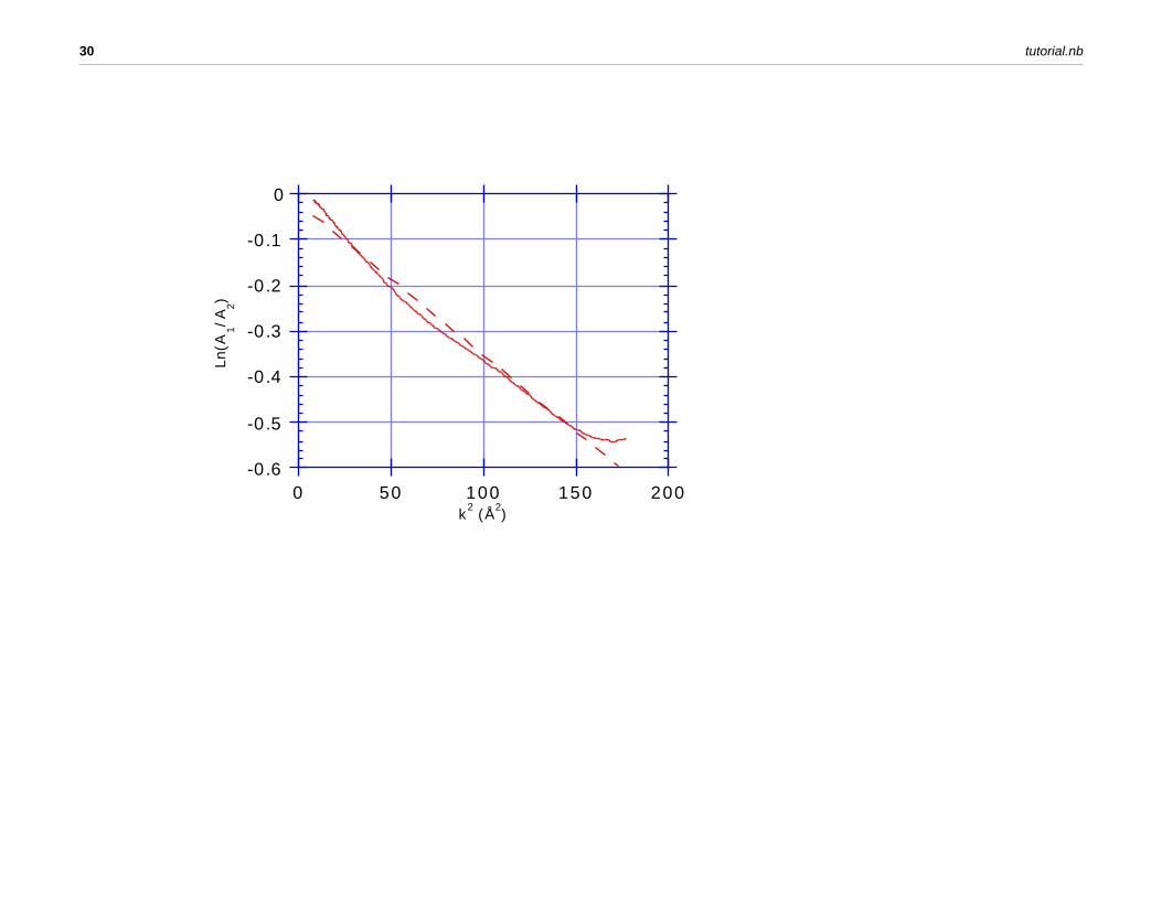
-0.6

-0.5

-0.4

-0.3

-0.2

-0.1

0Ln

(A1/A

2)

0 50 100 150 200k2 (Å2)

30 tutorial.nb

Types of systems for which XAFS is applicable

XAFS is applicable to condensed matter (both crystalline and amorphous), and molecular gases. Special conditions are not required - it is very suitable for in situ studies under real-life conditions. If a sample is oriented on a molecular or crystalline level, polarized EXAFS can provide information on 3D structure.

XANES can provide information about site symmetry, bond lengths, and orbital occupancy.

Limitations of and extensions to the EXAFS equation

Spherical waves

large disorder

multiple scattering

multielectron excitations

tutorial.nb 31

Elementary Interpretation of XANES

2: Experimental design and methods I

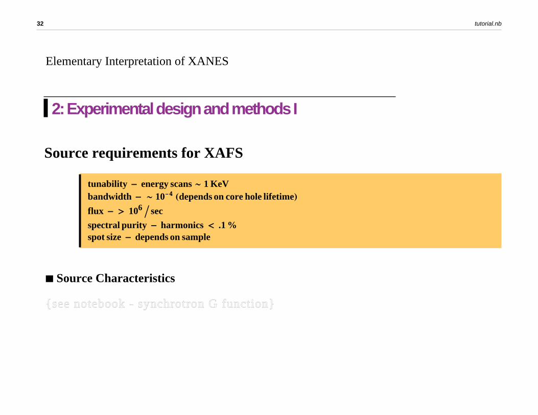
Source requirements for XAFS

tunability energy scans 1 KeVbandwidth 10 4 depends on core hole lifetime

flux 106 sec

spectral purity harmonics .1 %spot size depends on sample

Source Characteristics

{see notebook - synchrotron G function}

32 tutorial.nb

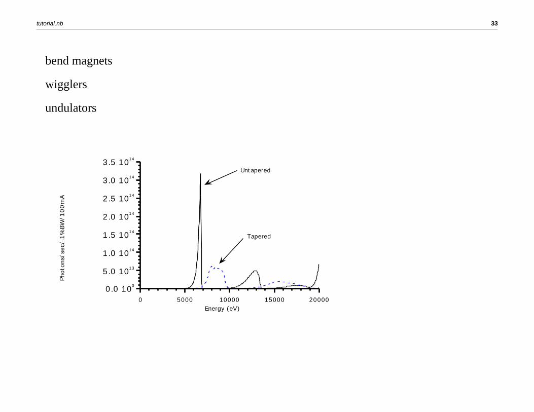
bend magnets

wigglers

undulators

0.0 100

5.0 1013

1.0 1014

1.5 1014

2.0 1014

2.5 1014

3.0 1014

3.5 1014

0 5000 10000 15000 20000

Tapered

Untapered

Energy (eV)

Phot

ons/

sec/

.1%

BW

/10

0m

A

tutorial.nb 33

Optics

monochromator types

double crystal monochromator -

lambda = 2 d Sin(theta); E = hc/2d Sin(theta)

variable exit - scan table to track beam motion

fixed exit - translate crystals internally to monochromator

sagittal focussing - bend second crystal to horizontally focus beam

harmonic rejection

crystal cuts (Si(111),Si(220),etc.)

{see notebook - Diamond Structure Factor}

34 tutorial.nb

detuning crystals

mirrors

Cross sections

photons absorbed/time = cross section * (intensity)

mu = Sum(rho_i*sigma_i)

tutorial.nb 35

Experimental modalities

transmission (scanning and dispersive)

geometry

detectors

fluorescence

geometry

detectors

filters

other devices

total external reflection fluorescence

electron yield

Polarized XAFS

36 tutorial.nb

How to minimize common experimental problems (HALO)

Harmonics

Alignment

Linearity

Offsets

Thickness/particle size effects

Sample requirements, preparation, sample cells

{see notebook - thickness effects}

choice of fill gases

tutorial.nb 37

3: Experimental design and methods II

Fluorescence mode

Amplitude corrections (fill gas etc)

Scattered Background

effective count rate

Experimental setup

Choosing a detector

Integrating detectors

Stern/Heald detector, PIN diodes, PMTs in current integration mode

Pulse counting detectors

Ge and Si detectors, APDs, PMTs

dead time corrections

38 tutorial.nb

using filters with Ge detector

Optimizing filters and slits

Q of filter

eta of slits

finding optimum

improved potential at the APS

Novel analyzers being developed

multilayer analyzer

Laue analyzer

Sample requirements, preparation, sample cells

Thick dilute limit

Thin concentrated limit

Problem with thick concentrated samples

tutorial.nb 39

use normal incidence geometry to improve

Total external reflection fluorescence

Survey of other methods: electron yield detection, reflectivity,

4: XAFS Theory I

Derivation of EXAFS equation

Dependence of amplitude and phase on Z

Importance of mean free path

Importance of single scattering plus focussing MS

Thermal disorder, Einstein and Debye Models

Disorder regimes

40 tutorial.nb

5: EXAFS Data Analysis I - EXAFS and disordered systems

Data reduction

Fourier filtering do's and don'ts

Cancellation of window effects

Ratio method

error estimates

Nonlinear least squares fitting

Pros and cons of R-space vs K-space fitting

Small disorder

moderate disorder

tutorial.nb 41

large disorder

Other methods (parametric models, splice, regularization)

6: XAFS Theory II

7: Data Analysis II: MS - XAFS and XANES

8: Recent developments, exotic methods, and future trends

DAFS

Magnetic XAFS, X-ray MCD

Photoconductivity

X-ray Raman

42 tutorial.nb

Optical detection

Acoustic detection

tutorial.nb 43