Introduction to Instrumental Variables Methods
71
Introduction to Instrumental Variables Methods Christian Hansen Booth School of Business University of Chicago
-
Upload
colt-hewitt -
Category
Documents
-
view
59 -
download
1
description
Introduction to Instrumental Variables Methods. Christian Hansen Booth School of Business University of Chicago. Introduction. Many studies in social sciences interested in inferring structural/causal/treatment effects Price elasticity of demand Effect of smoking on birthweight - PowerPoint PPT Presentation
Transcript of Introduction to Instrumental Variables Methods

Introduction to Instrumental Variables Methods
Christian HansenBooth School of Business
University of Chicago

Introduction• Many studies in social sciences interested in
inferring structural/causal/treatment effects– Price elasticity of demand– Effect of smoking on birthweight– Effect of 401(k) participation on saving– Effect of job training on wages/employment– Effect of schooling on wages– …
• Only have observational data
Conventional statistical methods may not recover desired effect

Example 1: Supply and Demand
Supply Curve
Demand CurveEquilibrium

Example 1: Supply and Demand
Suppose demand and supply fluctuate from day to day. We observe the market for several days and want to infer either the slope of the supply or demand curve (from which economic quantities such as demand elasticity are derived).

Example 1: Supply and Demand
Suppose demand and supply fluctuate from day to day. We observe the market for several days and want to infer either the slope of the supply or demand curve (from which economic quantities such as demand elasticity are derived).
Observed relationship between price and quantity reveals neither supply nor demand! (Simultaneity)

Example 2: Job Training• Observe data on earnings for people who have and have not
completed job training.• Want to infer the causal effect of job training on earnings
• What if people who are more “motivated” are more likely to get training and on average earn more than less “motivated”?
‒ Difference between average earnings across the trained and untrained confounds the effects of motivation and training
‒ Omitted variables bias: Would like to control for unobserved (and unobservable?) motivation

Example 3: Classical Measurement Error• Model: . Want to know the effect of x on y (β)• Only observe noisy signal for x:
• What do you get from regressing on ?
• The last term generally does not have 0 expectation or converge to 0 even in large samples
• Under “classical measurement error” () the second term converges to (attenuation bias)
2
2 2v
v x

Common Structure:
• “Structural” Model:
• y – outcome of interest• x – observed “treatment” variable• – treatment/structural/causal effect (NOT
regression coefficient)• (Endogeneity)
Instrumental variables (IV) offers one approach to estimating (when instruments are available…)

What is an instrument?
• Instrumental variable (denoted ) shifts but is unrelated to structural error (). – (relevance)– (exclusion)
• Intuition: Movements in are unrelated to movements in but are related to movements in
Movements in “induced” by are uncontaminated. Can be used to estimate treatment effect.
Key statistical conditions

How do instruments help?• Consider supply/demand example:
• is a variable that affects supply (but not demand (say the price of a factor of production). .– Valid instrument for demand.

How do instruments help?• Heuristic: When changes:
– supply changes– demand remains the same (on average)
Movements in the supply curve induced by changing z trace out the demand curve

How do instruments help?• Quasi-mathematically. IV model
• Recall OLS estimator: – Neither unbiased nor consistent since

How do instruments help?• IV estimator:
– Uses only uncontaminated variation (covariation between instrument and X and instrument and Y)
– Under conditions above (plus regularity), generally consistent, asymptotically normal with estimable covariance matrix.
– Software: (Also really easy to code yourself)• Stata: ivregress (and variants)• SAS: proc syslin (and others)• R: sem package• SPSS: Analyze -> Regression -> Two-stage least squares• …

Questions?• Where do instruments come from?
– Intuition, subject matter knowledge, randomization• Can I assess the validity of the underlying assumptions?
– Sort of, is fundamentally untestable (though aspects can be tested if extra instruments available)
– is testable• What if I have extra instruments (so Z’X is not
invertible)?– Two-stage least squares (2SLS). Same intuition. Default
implementation in all stats packages. Other options• Are there things I should look out for?
– Weak instruments. Many instruments. Reasons to doubt the exclusion restriction. What exactly is estimated when treatment effects are heterogeneous.

Example: Job Training• Goal: Assess impact of job training on subsequent labor
market outcomes (e.g. employment, wages)
• Problem: Training receipt is not randomly assigned. May be endogenous.– E.g. maybe more motivated people more likely to receive job
training and more likely to find subsequent employment/have better job performance
• Instrument: Under Job Training Partnership Act (JTPA), randomized trial conducted in which individuals offered JTPA services– Use JTPA offer of services as instrument for receiving training

Example: Job Training• Plausibility of instrument:– Offer of services randomly assigned => Independent of
structural error by construction. (No evidence about this in data)
– ≈ 60% of those offered training accepted offer => Offer strongly related to receipt. (Can look at correlation between instrument and endogenous variable to assess this)
• Aside: One could simply regress outcome on offer of treatment to estimate intention-to-treat (ITT). Our goal is to estimate effect of treatment, not offer.

Example: Job Training• Structural Equation:
• First-Stage Equation:
– Regression of treatment on instrument and controls– Note: E[zixi] ≠ 0 => π1,z ≠ 0
• Reduced Form Equation:
– Regression of outcome on instrument and controls– Note: If can’t rule out π2,z = 0, can’t rule out α = 0
• First-stage and reduced form are predictive representations, not structural . Good practice to report results from all three.

Example: Job Training• Variables:
– Earn – total earnings over 30 month period following assignment of offer
– Train – dummy for receipt of job training services– Offer – dummy for offer to receive training services– x – 13 additional control variables
• dummies for black and Hispanic persons, a dummy indicating high-school graduates and GED holders, five age-group dummies, a marital status dummy, a dummy indicating whether the applicant worked 12 or more weeks in the 12 months prior to the assignment, a dummy signifying that earnings data are from a second follow-up survey, and dummies for the recommended service strategy

Example: Job Training• OLS Results (from Stata):
regress earnings train x1-x13 , robust
Linear regression Number of obs = 5102 F( 14, 5087) = 38.35 Prob > F = 0.0000 R-squared = 0.0909 Root MSE = 18659
------------------------------------------------------------------------------ | Robust earnings | Coef. Std. Err. t P>|t| [95% Conf. Interval]-------------+---------------------------------------------------------------- train | 3753.362 536.3832 7.00 0.000 2701.82 4804.904...
If intuition about source of endogeneity is correct, this should be an over-estimate of the effect of training.

Example: Job Training• First-Stage Results (from Stata):
regress train offer x1-x13 , robust
Linear regression Number of obs = 5102 F( 14, 5087) = 390.75 Prob > F = 0.0000 R-squared = 0.3570 Root MSE = .39619
------------------------------------------------------------------------------ | Robust train | Coef. Std. Err. t P>|t| [95% Conf. Interval]-------------+---------------------------------------------------------------- offer | .6088885 .0087478 69.60 0.000 .591739 .6260379...
Strong evidence that E[zixi] ≠ 0

Example: Job Training• Reduced-Form Results (from Stata):
regress earnings offer x1-x13 , robust
Linear regression Number of obs = 5102 F( 14, 5087) = 34.19 Prob > F = 0.0000 R-squared = 0.0826 Root MSE = 18744
------------------------------------------------------------------------------ | Robust earnings | Coef. Std. Err. t P>|t| [95% Conf. Interval]-------------+---------------------------------------------------------------- offer | 970.043 545.6179 1.78 0.075 -99.60296 2039.689....
Moderate evidence of a non-zero treatment effect (maintaining exclusion restriction)

Example: Job Training• IV Results (from Stata):
ivreg earnings (train = offer) x1-x13 , robust
Instrumental variables (2SLS) regression Number of obs = 5102 F( 14, 5087) = 34.38 Prob > F = 0.0000 R-squared = 0.0879 Root MSE = 18689
------------------------------------------------------------------------------ | Robust earnings | Coef. Std. Err. t P>|t| [95% Conf. Interval]-------------+---------------------------------------------------------------- train | 1593.137 894.7528 1.78 0.075 -160.9632 3347.238...
Moderate evidence of a positive treatment effect (maintaining exclusion restriction). Substantially attenuated relative to OLS, consistent with intuition.
Note: Some software reports R2 after IV regression. This object is NOT meaningful and should not be used.

Two-Stage Least Squares• May have more instruments than endogenous variables• In principle, many IV estimators can be constructed• 2SLS is the minimum variance (under homoskedasticity) linear
combination of the potential IV estimators (otherwise may use GMM)• 2SLS is the GMM estimator using the full set of orthogonality conditions
implied by • 2SLS and IV are numerically equivalent when # of endogenous variables = # of instruments• Aside: Some jargon
– r = # of instruments, k = # of endogenous variables– r = k, “just-identified”– r > k, “over-identified”

2SLS• 2SLS estimator:
– PZ = Z(Z’Z)-1Z’, projection matrix onto Z– Uses only uncontaminated variation (covariation between instrument
and X and instrument and Y)– Under conditions above (plus regularity), generally consistent,
asymptotically normal with estimable covariance matrix.– Can be viewed as two-step procedure where endogenous variables and
outcomes are first projected onto Z and then projections are used in OLS
– Software: (Also really easy to code yourself)• Stata: ivregress (and variants)• SAS: proc syslin (and others)• R: sem package• SPSS: Analyze -> Regression -> Two-stage least squares• …

Testing Overidentifying Restrictions• Have more instruments than we need to estimate the
treatment effect
• If all instruments satisfy exclusion restriction, all subsets should (asymptotically) return the same estimate of the treatment effect
• Idea: Obtain multiple estimates of the treatment effect and test that they are the same.
• Rejection implies some subset of exclusion restrictions may be invalid

Hansen’s Over-Identification Test• Also called the “J-Test”, Sargan test, “S-Test”• Based on GMM criterion function
• For IID, homoskedastic data:
(More generally, J is GMM objective function evaluated at GMM point-estimate)

Overidentification Tests:• Can never tell you that the exclusion restriction ( is
satisfied– Failure to reject does not imply true– Even if it did, only learn that probability limits of various IV
estimators are the same. Maybe all the same and wrong. – Heterogeneous treatment effects?
• Rejection indicates that some subset of instruments may be invalid– Does not indicate which subset– Does not mean all exclusion restrictions are invalid– Heterogeneous treatment effects?

Example: Returns to Schooling• Goal: Estimate the value added of additional
years of schooling in terms of wages
• Problem: Years of completed schooling is not randomly assigned. May be endogenous.– E.g. maybe academic ability is related to qualities
that relate to job performance/salary (motivation, intelligence, task orientation, etc.)
• Instrument: Quarter of birth (Angrist and Krueger, 1991)

Example: Returns to Schooling• Plausibility of instrument:
– Compulsory schooling laws in the U.S. are typically based on age, not number of years of school. People born at different times of the year can drop out after receiving different amounts of school. (Can look at correlation between instrument and endogenous variable to assess this)
– When a person is born is unrelated to inherent traits (e.g. motivation, intelligence, …) and so should not have a direct effect on wages but only affect wages through the relationship to completed schooling induced by compulsory education laws.• Untestable, but we do have overidentifying restrictions coming from different
birth quarters. • Validity has been questioned. E.g. winter birth may be correlated to
increased exposure to early health problems; more conscientious parents may respond by timing birth; …

Example: Returns to Schooling• Structural Equation:
• First-Stage Equation:
– Note: E[zixi] ≠ 0 => π1,1 ≠ 0 or π1,2 ≠ 0 or π1,3 ≠ 0
• Reduced Form Equation:

Example: Returns to Schooling• Data from 1980 Census for men aged 40-49 in 1980• Variables:
– Wage – hourly wage– School – reported years of completed schooling– Q1-Q3 – dummies for quarter of birth– x – 59 control variables. Dummies for state of birth and year of
birth
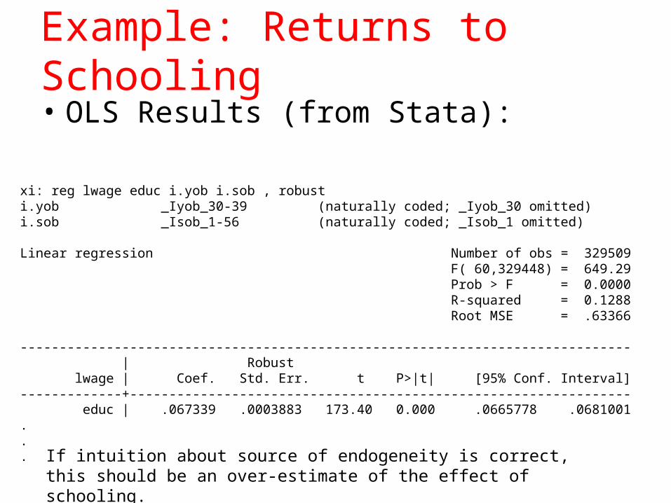
Example: Returns to Schooling• OLS Results (from Stata):
xi: reg lwage educ i.yob i.sob , robusti.yob _Iyob_30-39 (naturally coded; _Iyob_30 omitted)i.sob _Isob_1-56 (naturally coded; _Isob_1 omitted)
Linear regression Number of obs = 329509 F( 60,329448) = 649.29 Prob > F = 0.0000 R-squared = 0.1288 Root MSE = .63366
------------------------------------------------------------------------------ | Robust lwage | Coef. Std. Err. t P>|t| [95% Conf. Interval]-------------+---------------------------------------------------------------- educ | .067339 .0003883 173.40 0.000 .0665778 .0681001... If intuition about source of endogeneity is correct, this should be an over-
estimate of the effect of schooling.

Example: Returns to Schooling• First-Stage Results (from Stata):
xi: regress educ i.qob i.sob i.yob , robustLinear regression Number of obs = 329509 F( 62,329446) = 292.87 Prob > F = 0.0000 R-squared = 0.0572 Root MSE = 3.1863
------------------------------------------------------------------------------ | Robust educ | Coef. Std. Err. t P>|t| [95% Conf. Interval]-------------+---------------------------------------------------------------- _Iqob_2 | .0455652 .015977 2.85 0.004 .0142508 .0768797 _Iqob_3 | .1060082 .0155308 6.83 0.000 .0755683 .136448 _Iqob_4 | .1525798 .0157993 9.66 0.000 .1216137 .1835459
.
.
. testparm _Iqob*
( 1) _Iqob_2 = 0 ( 2) _Iqob_3 = 0 ( 3) _Iqob_4 = 0
F( 3,329446) = 36.06 Prob > F = 0.0000
First-stage F-statistic.

Example: Returns to Schooling• Reduced-Form Results (from Stata):
xi: regress lwage i.qob i.sob i.yob , robust
Linear regression Number of obs = 329509 F( 62,329446) = 147.83 Prob > F = 0.0000 R-squared = 0.0290 Root MSE = .66899
------------------------------------------------------------------------------ | Robust lwage | Coef. Std. Err. t P>|t| [95% Conf. Interval]-------------+---------------------------------------------------------------- _Iqob_2 | .0028362 .0033445 0.85 0.396 -.0037188 .0093912 _Iqob_3 | .0141472 .0032519 4.35 0.000 .0077736 .0205207 _Iqob_4 | .0144615 .0033236 4.35 0.000 .0079472 .0209757..
testparm _Iqob*
( 1) _Iqob_2 = 0 ( 2) _Iqob_3 = 0 ( 3) _Iqob_4 = 0
F( 3,329446) = 10.43 Prob > F = 0.0000

Example: Returns to Schooling• 2SLS Results (from Stata):
xi: ivregress 2sls lwage (educ = i.qob) i.yob i.sob , robust
Instrumental variables (2SLS) regression Number of obs = 329509 Wald chi2(60) = 9996.12 Prob > chi2 = 0.0000 R-squared = 0.0929 Root MSE = .64652
------------------------------------------------------------------------------ | Robust lwage | Coef. Std. Err. z P>|z| [95% Conf. Interval]-------------+---------------------------------------------------------------- educ | .1076937 .0195571 5.51 0.000 .0693624 .146025...
Bigger than OLS?

Example: Returns to Schooling• GMM Results (from Stata, efficient under heteroskedasticity):
xi: ivregress gmm lwage (educ = i.qob) i.yob i.sob , robust
Instrumental variables (GMM) regression Number of obs = 329509 Wald chi2(60) = 9992.90 Prob > chi2 = 0.0000 R-squared = 0.0927GMM weight matrix: Robust Root MSE = .64658
------------------------------------------------------------------------------ | Robust lwage | Coef. Std. Err. z P>|z| [95% Conf. Interval]-------------+---------------------------------------------------------------- educ | .1077817 .0195588 5.51 0.000 .0694472 .1461163...
estat overid
Test of overidentifying restriction:
Hansen's J chi2(2) = 3.10009 (p = 0.2122)
Bigger than OLS?
Fail to reject over-id test

Heterogeneous Treatment Effects: ATE
• Previous discussion posits a constant treatment/structural effect
• Estimated constant treatment effect = average treatment effect (ATE) sometimes
– independent of and , =>– where
– i.e. IV model holds interpreting parameter as ATE– Note: Exclusion restriction will not hold in general if
heterogeneous effect is not independent of instrument or treatment!

Heterogeneous Treatment Effects: LATE
• When heterogeneous effect is not independent, can still estimate a causal effect among a subpopulation
• Strip model down to binary treatment and binary instrument
• Four subpopulations:– Always-takers: zi = 1, xi = 1 and zi = 0, xi = 1
– Never-takers: zi = 1, xi = 0 and zi = 0, xi = 0
– Complier: zi = 1, xi = 1 and zi = 0, xi = 0
– Defier: zi = 1, xi = 0 and zi = 0, xi = 1– Note: Never observe individuals at both instrument states. Can’t
determine observation’s subpopulation

Heterogeneous Treatment Effects: LATE
• Generally, may estimate ATE among subpopulation of compliers– Termed Local Average Treatment Effect (LATE)
• Conditions:– Independence – instrument independent of all unobservables
affecting outcome and treatment/endogenous variable state– Exclusion – instrument only affects outcome though treatment
receipt. (No direct effect of the instrument.)– First-stage – instrument predicts treatment receipt– Monotonicity – effect of instrument on probability of receiving
treatment is ≥ 0 for everyone or ≤ 0 for everyone. (No defiers)
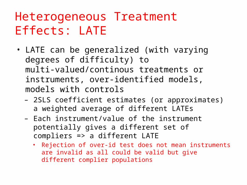
Heterogeneous Treatment Effects: LATE
• LATE can be generalized (with varying degrees of difficulty) to multi-valued/continous treatments or instruments, over-identified models, models with controls– 2SLS coefficient estimates (or approximates) a
weighted average of different LATEs– Each instrument/value of the instrument potentially
gives a different set of compliers => a different LATE• Rejection of over-id test does not mean instruments are
invalid as all could be valid but give different complier populations

Heterogeneous Treatment Effects: LATE
• Can learn some things about compliers from data
• A couple simple ones:– Size of complier population:
– Proportion of treated who are compliers:
Probability complier or always-taker
Probability always-taker. No defiers

Example: JTPA• Recall treatment = dummy for receipt of job training
services• Instrument = dummy for offer to receive training services• Size of complier group ≈ 61% • Proportion of treated (those who received training) who are
compliers ≈ (.67/.42)*.61 ≈ .97• IV estimate of training effect: 1593.14 (894.75)• Seems plausible that there are no defiers• Compliers = people who would not receive training if not
offered but choose to have training when offered• Presumably, the remaining 39% of the population are
mostly never-takers

Example: Returns to Schooling• Returns to schooling more complicated
– Multi-valued treatment– Multiple instruments
• IV estimand with one binary instrument = weighted average of effects of increasing schooling by one year across all schooling levels among compliers
• 2SLS estimand = weighted average of individual IV estimands
• Monotonicity condition => change in instrument leads to weakly increasing (decreasing) levels of schooling for everyone

Example: Returns to Schooling• Consider dummy for being born quarter j (qj)
• Maintain exclusion restriction as before
• First-stage: Regress schooling on qj
• Can estimate fraction of compliers at each schooling level as P(si < s|qji = 0) – P(si < s|qji = 1) (Assuming monotonicity such that changing instrument from 0 to 1 increases schooling)
• Can estimate weight given to each schooling value as (fraction of compliers)/first-stage
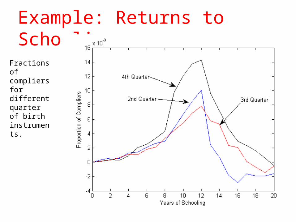
Example: Returns to Schooling
Fractions of compliers for different quarter of birth instruments.

Example: Returns to Schooling
Weighting functions for different quarter of birth instruments. Note this is the fraction of compliers scaled by the first-stage coefficient.

Example: Returns to Schooling• OLS Estimate: .067 (.0004)
• IV Estimates:– Q2: .166 (.071)– Q3: .209 (.076)– Q4: .085 (.026)
• 2SLS Estimate: .108 (.020) [Weighted average of the individual IV estimates]
• Compliers: People who got more school due to being born later in the year. Margin is mostly in 10-12 years of education.

Many Instruments• IV Estimates often imprecise– Only use the variation induced by the instrument– Often plausible instruments (in the sense of satisfying the
exclusion restriction) have weak predictive power for outcome
• One approach to increasing precision is to use more instruments– Potentially allow extraction of more signal, adding
information helps• But…– Are all the instruments really excludable?– Overfitting is bad

Many Instruments: Overfitting• Extreme case, # instruments (K) = # observations (n)
• Recall where PZ = Z(Z’Z)-1Z’– K=n => (Z’Z)-1 = Z-1(Z’)-1 => PZ = I (the identity matrix)– So
• Get back original, contaminated object since perfectly fit both signal AND noise. – Overfitting fits contaminated noise as well as signal
�̂�2𝑆𝐿𝑆= (𝑋 ′𝑃 𝑍 𝑋 )−1 ( 𝑋′ 𝑃 𝑍𝑌 )=(𝑋 ′ 𝑋 )−1 (𝑋′𝑌 )= �̂�𝑂𝐿𝑆

Example: Returns to Schooling• Rather than just use 3 quarter of birth effects, could
use quarter of birth interacted with year of birth x state of birth as instruments (1527 instruments)
• 2SLS estimate: .0712 (.0049)– Recall OLS gives .067 (.0004) and 2SLS with 3 quarter of
birth dummies gives .108 (.020)
• Theory, simulation evidence, the intuition above suggests 2SLS is strongly biased towards OLS when many instruments are used

Many Instruments: Solutions• Use less instruments
– Use model selection techniques in the first-stage to choose a good set
• Use an estimator that is less sensitive to first-stage overfitting– Limited information maximum likelihood (LIML), Fuller, Jackknife
Instrumental Variables (JIVE)– Need to adjust standard errors to account for first-stage
overfitting
• Use an estimator that is less sensitive to first-stage overfitting and regularize the first-stage– Regularized Jackknife Instrumental Variables (RJIVE)

Example: Returns to Schooling• 1527 instruments again– 2SLS estimate: .0712 (.0049)– 2SLS (3 instrument): .108 (.020)– OLS gives .067 (.0004)
– Use LASSO to select variables that predict schooling from among 1527 variables. Use these variables as instruments: .0862 (.0254)
– JIVE: .0816 (.5168)– RJIVE: .1067 (.0171)

Example: Eminent Domain
• Estimate economic consequences of the law of takings or eminent domain
• Potential impacts:– ``public use'' - removing economic blight and/or promoting
economic development– redistribution of wealth from groups with little political power – distortions in the efficient investment of capital
• underinvestment due to uncertainty induced by potential seizure• overinvestment when property owners anticipate receiving higher
than market compensation

Example: Eminent Domain
• Want to understand effect of number of decisions that favor private ownership (go against government seizure) on economic outcomes– Real estate prices, GDP
• Legal decisions may be related to these variables. Potential endogeneity.– property values provide signal about ``public use''
• low property values: poor prospects, blight• high property values: viability of a redevelopment or commercial
project
– decisions in other areas of law may affect economic outcomes and generate precedent/influence decisions related to takings
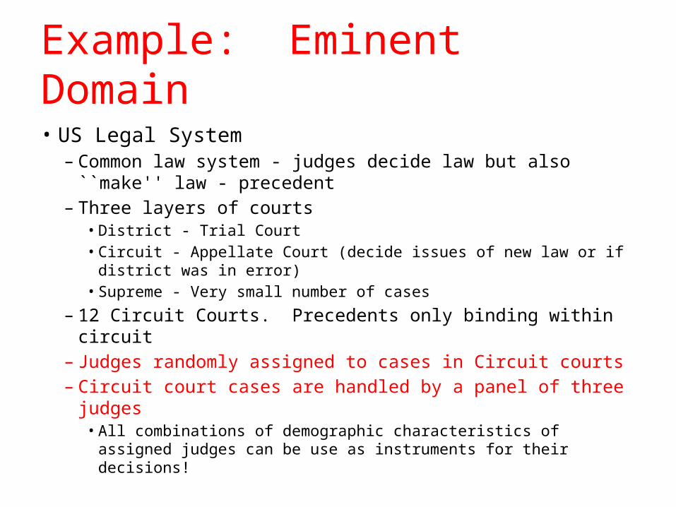
Example: Eminent Domain
• US Legal System– Common law system - judges decide law but also ``make''
law - precedent– Three layers of courts
• District - Trial Court• Circuit - Appellate Court (decide issues of new law or if district
was in error)• Supreme - Very small number of cases
– 12 Circuit Courts. Precedents only binding within circuit– Judges randomly assigned to cases in Circuit courts– Circuit court cases are handled by a panel of three judges
• All combinations of demographic characteristics of assigned judges can be use as instruments for their decisions!

Example: Eminent Domain
• Problem: Too many instruments– Have between 110-312 observations depending
on outcome– Have between 138 and 147 instruments
depending on the outcome– Also have between 30 and 33 controls depending
on outcome– Use LASSO (variable selection) to select a small set
of instruments

Example: Eminent Domain• Results:
– log(FHFA House Price Index): • OLS: .011 (.013)• 2SLS (after LASSO): .037 (.047) (1 instrument selected)
– log(non-metro House Price Index):• OLS: .011 (.007)• 2SLS (after LASSO): .036 (.013) (4 instruments selected)
– log(Case-Shiller House Price Index):• OLS: .015 (.013)• 2SLS (after LASSO): .063 (.025) (2 instruments selected)
– log(GDP):• OLS: .0099 (.0048)• 2SLS (after LASSO): .013 (.016) (1 instrument selected)
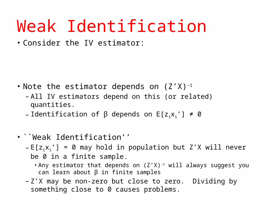
Weak Identification• Consider the IV estimator:
• Note the estimator depends on (Z’X)-1
– All IV estimators depend on this (or related) quantities. – Identification of β depends on E[zixi’] ≠ 0
• ``Weak Identification’’– E[zixi’] = 0 may hold in population but Z’X will never be 0 in a finite
sample.• Any estimator that depends on (Z’X)-1 will always suggest you can learn about
β in finite samples– Z’X may be non-zero but close to zero. Dividing by something close to
0 causes problems.

Weak Identification• Extreme case as an illustration:
• IV estimator inconsistent (so are its variants)• Asymptotic distribution complicated (easy to
simulate)• Note if , , so – Inconsistent and centered at probability limit of OLS.

Weak Identification• What to do?
– Consistent estimation not possible if correlation between Z and X small
1. Always look at first-stage statistics– Want strong relationship between instrument (big t/F statistic on
instruments)– Not clear how big. Simulations suggest |t| > 6 not a bad rule of
thumb when dim(z) = dim(x) = 1
2. Forget estimation. Focus on inference that doesn’t depend on (Z’X)-1 – Various options. See references.– Involves inverting test-statistics (usually by grid search). May be
computationally demanding, especially when dim(x) bigger than a few

Weak Identification• One simple approach:
– Suppose you knew the actual treatment effect• Call it
– Consider the equation
– From the exclusion restriction, we know since we are evaluating at the true values
• Algorithm based on this idea:1. Hypothesize value for , say 2. Form 3. Regress on to obtain 4. Test at your favorite level, α, (say 5%) using your favorite test (say an F-test)
– If you reject, reject as a potential value of the treatment effect at the α-level– If you fail to reject, include in the (1-α)% confidence interval
5. Repeat steps 1-4 for a set of J candidate values . Construct the (1-α)% confidence interval as the set of values that are not rejected.

Example: Effects of Institutions on Economic Growth
• Want to understand the effect of “institutions” on economic output
• Complicated due to potential joint determination– Do high quality institutions lead to more growth?– Does more economic development lead to better institutions?
• Instrument: European settler mortality (i.e. 1500’s-1600’s)– Idea: Europeans set up better institutions in places they
wanted to live. Institutions are persistent.– How often settlers died hundreds of years ago shouldn’t affect
growth except through institutions (maybe need to control for geography, resources, …)
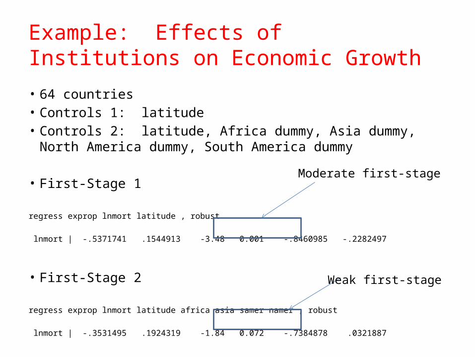
Example: Effects of Institutions on Economic Growth
• 64 countries• Controls 1: latitude• Controls 2: latitude, Africa dummy, Asia dummy, North America
dummy, South America dummy
• First-Stage 1
regress exprop lnmort latitude , robust
lnmort | -.5371741 .1544913 -3.48 0.001 -.8460985 -.2282497
• First-Stage 2
regress exprop lnmort latitude africa asia samer namer , robust
lnmort | -.3531495 .1924319 -1.84 0.072 -.7384878 .0321887
Weak first-stage
Moderate first-stage

Example: Effects of Institutions on Economic Growth
• IV 1ivregress 2sls gdp (exprop = lnmort) latitude , robust
exprop | .9692383 .2077791 4.66 0.000 .5619988 1.376478
• IV 2ivregress 2sls gdp (exprop = lnmort) latitude africa asia namer samer , robust
exprop | 1.036001 .450362 2.30 0.021 .1533074 1.918694
Based on strong identification

Example: Effects of Institutions on Economic Growth
• Test 1. Controls 1:
regress gdp lnmort latitude , robust
lnmort | -.5206497 .0830659 -6.27 0.000 -.6867503 -.3545491
2. Controls 2:
regress gdp lnmort latitude africa asia namer samer , robust
lnmort | -.3658632 .1343732 -2.72 0.009 -.6349408 -.0967855
Reject
Reject

Example: Effects of Institutions on Economic Growth
• Test gen newy = gdp - 2*exprop
1. Controls 1:regress newy lnmort latitude , robust
lnmort | .5536985 .2623656 2.11 0.039 .029066 1.078331
2. Controls 2:
regress newy lnmort latitude africa asia namer samer , robust
lnmort | .3404359 .3307904 1.03 0.308 -.3219604 1.002832
Reject
Fail to Reject
Create new dependent variable

Example: Effects of Institutions on Economic Growth
• Repeating the exercise on the previous two slides for many different hypothesized values of , we can construct approximate 95% confidence intervals– Controls 1: • Regular Asymptotic: (0.56,1.38)• Weak identification robust: (0.68,1.83)
– Controls 2:• Regular Asymptotic: (0.15,1.92)• Weak identification robust: (-,-8.93) U (.41,)

Short List of References
• Textbooks:– Hayashi, Econometrics, Ch. 3– Wooldridge, Econometric Analysis of Cross Section
and Panel Data, Ch. 5, 6.2– Angrist and Pischke, Mostly Harmless
Econometrics, Ch. 4

Short List of References
• Papers - Applications:– Abadie, A., Angrist, J., Imbens, G., 2002. Instrumental variables
estimates of the effect of subsidized training on the quantiles of trainee earnings. Econometrica, 70, 91–117.
– Acemoglu, D., Johnson, S., and Robinson, J. A., 2001, “The Colonial Origins of Comparative Development: An Empirical Investigation,” American Economic Review, 91, 1369-1401.
– Angrist, J. D. and A. Krueger, 1991, “Does Compulsory Schooling Attendance Affect Schooling and Earnings,” Quarterly Journal of Economics, 106, 979-1014.
– Belloni, A., Chen, D., Chernozhukov, V., and C. Hansen “Sparse Models and Methods for Optimal Instruments with an Application to Eminent Domain” forthcoming Econometrica

Short List of References• Papers – Heterogeneous Treatment Effects:
– Angrist, J. (2004) “Treatment Effect Heterogeneity in Theory and Practice,” The Economic Journal 114, C52-C83.
– Angrist, J. (2005) “Instrumental Variables in Experimental Criminological Research: What, Why, and How,” Journal of Experimental Criminological Research 2, 1-22.
– Angrist, J., G. Imbens, and D. Rubin, (1996) “Identification of Causal effects Using Instrumental Variables,” with comments and rejoinder, Journal of the American Statistical Association.
– Imbens, G. and J. Angrist, (1994) “Identification and Estimation of Local Average Treatment Effects,” Econometrica.
– Card, D. (1999) "The Causal Effect of Education on Earnings," The Handbook of Labor Economics, Volume IIIA, Elsevier Science Publishers.

Short List of References• Papers – Weak and Many Instruments:
– Andrews, D. W. K.., M. J. Moreira, and J. H. Stock, 2006, “Optimal Two-Sided Invariant Similar Tests for Instrumental Variables Regression,” Econometrica, 74, 715-752.
– Belloni, A., Chen, D., Chernozhukov, V., and C. Hansen “Sparse Models and Methods for Optimal Instruments with an Application to Eminent Domain” forthcoming Econometrica
– Bekker, P. A., 1994, “Alternative Approximations to the Distributions of Instrumental Variables Estimators,” Econometrica, 63, 657-681.
– Chernozhukov, V. and C. Hansen, 2008, “The Reduced Form: A Simple Approach to Inference with Weak Instruments,” Economics Letters, 100, 68-71.
– Hahn, J., J. A. Hausman, and G. M. Kuersteiner, 2004, “Estimation with Weak Instruments: Accuracy of Higher-Order Bias and MSE Approximations,” Econometrics Journal, 7, 272-306.
– Hansen, C., J. A. Hausman, and W. K. Newey, 2008, “Estimation with Many Instrumental Variables,” Journal of Business and Economic Statistics, 26, 398-422.
– Hansen, C. and D. Kozbur, 2012, “Instrumental Variables Estimation With Many Weak Instruments Using Regularized JIVE,” working paper (available at http://faculty.chicagobooth.edu/christian.hansen/research/)
– Kleibergen, F., 2002, “Pivotal Statistics for Testing Structural Parameters in Instrumental Variables Regression,” Econometrica, 70, 1781-1803.
– Kleibergen, F., 2007, “Generalizing Weak Instrument Robust IV Statistics towards Multiple Parameters, Unrestricted Covariance Matrices, and Identification Statistics,” Journal of Econometrics, 139, 181-216.
– Moreira, M. J., 2003, “A Conditional Likelihood Ratio Test for Structural Models,” Econometrica, 71, 1027-1048.
– Staiger, D. and J. Stock, 1997, “Instrumental Variables Regression with Weak Instruments,” Econometrica, 65, 557-586.
– Stock, J., J. H. Wright, and M. Yogo, 2002, “A Survey of Weak Instruments and Weak Identification in Generalized Method of Moments,” Journal of Business and Economic Statistics, 20, 518-529.


![Unbiased Testing Under Weak Instrumental Variables€¦ · Unbiased Testing Under Weak Instrumental Variables Abstract ThispaperfindsunbiasedtestsusingthreeofNagar’s[1959]k-classestimators:](https://static.fdocuments.us/doc/165x107/5e9970e0d7bf8a424c633a60/unbiased-testing-under-weak-instrumental-variables-unbiased-testing-under-weak-instrumental.jpg)