Introduction to IBM DB2

To Introduce Basic Database Management System in preparation to IBM DB2

Why IBM DB2?

Who uses DB2?

What is an RDBMS?

3 levels of data model

DB2 database software offers industry leading performance, scale, and reliability on your choice of platform from Linux, Unix and Windows to z/OS

Italian transportation company

Coca-Cola Bottling Co.

WAZ Media Group

Italian transportation company

Industry: Travel and Transportation

Excerpt: "We chose SAP solutions because they integrate seamlessly with our existing SAP general business management and financial software." - IT Technical Manager, Transportation Company

Coca-Cola Bottling Co. Industry: Beverages Excerpt: "In 2008, Coca-Cola Bottling Co.

Consolidated (CCBCC) faced a technical upgrade of its ERP system. In light of the SAP DB2 licensing agreement with The Cocal-Cola Company (TCCC), CCBCC decided to migrate its database system to DB2. The move has brought about a 40% reduction in database storage space, which helps to decelerate the company's data volume growth. This was translated into a predicted savings of US$750,000 over five years in terms of licensing and maintenance cost."

WAZ Media Group

Industry: Media & Entertainment

Excerpt: "While in the past we had to wait hours for some analyses of large data volumes, today they are ready within a minute. Thus, the new technology is immediately being transformed into commercial success. And the great flexibility of the IBM SPSS Modeler solution offers us huge future potential." - Dr. Ana Moya, Sales Management, Reporting and Analysis department, WAZ

Data is a collection of letters, numbers or facts

Information is a processed data that provides a value

File - is a collection of records

DB (Database) – an organized collection of data used by various applications

DBMS (Database Management System) – is a software system that manages execution of users applications to access/modify data

RDBMS (Relational DBMS) – based on the relational model; which defines a relationship between tables in the database ands eliminates unnecessary data redundancy

Tables - is a set of data elements (values) that is organized using a model of vertical columns (name) and horizontal rows (values) :wikipedia

Students

Subjects Taken

Stud_ID Stud_Name Course

14A-1710-261 Jomar Salvador BSIT

14A-1711-261 Rachelle Taopa BSBA

Stud_ID Subject Code

14A-1710-261 ITCS220

14A-1710-261 ITCS121

14A-1711-261 ENG +

Commercially available DBMS: ◦ Commercial software is computer software that is

produced for sale (payware) or for free (open source software) or that serves commercial purposes.

IBM DB2

Oracle

Microsoft SQL Server

Sybase

MySQL

Physical – How data is stored, accessed, modified, ordered, and how they are represented (ASCII, Unicode, etc.)

Conceptual – what the data express and what relationships the data expresses

View – what part of the data is seen by a specific application

External schema ◦ usually comes from the application design

process but that can be a good starting point for data modeling.

◦ shows how your system will be used. A common way to show the external schema is by using UML Use Case diagrams.

Determine the purpose of your database

Find and organize the required information

Divide the information into tables

Turn information items into columns

Specify primary keys

Setup table relationships

Refine your design

Apply normalization rules

Table normalization - Lack of 3NF leads to update, insert, and delete anomalies.

this will reduce data redundancy and wrong assignment of primary key

Fixed width text fields too large - Datatype of char(255) where a smaller width or varchar should be used

Improper grouping in queries - With proper keys on tables, improper grouping makes itself more apparent

What is normalization?

Normalization is the process of efficiently organizing data in the database by eliminating redundant data and ensuring data dependencies make sense.

The normal forms

these are guidelines for ensuring that databases are normalized; numbered from 1 (1NF) to 5 (5NF)

First normal Form (1NF) ◦ Eliminate duplicate columns from the same table

◦ Create separate tables for each group of related data and identify each row with a unique column (the primary key)

Reg_ID Stud_ID

001 14A-1710-261

001 14A-1711-262

001 14A-1711-263

Stud_ID Stud_Name

14A-1710-261 Jomar Salvador

14A-1711-262 Rachelle Taopa

14A-1711-263 Peachy Sison

Second Normal Form (2NF) ◦ Remove subsets of data that apply to multiple rows

and place them in a separate table

◦ Create relationships between these tables through the use of foreign keys.

Stud_ID FirstN LastN Address City State Zipcode

14A-1710-261

Jomar Salvador Bangkulasi Navotas Philippines 1485

Stud_ID FirstName LastName Address Zipcode

14A-1710-261

Jomar Salvador Bangkulasi 1485

Zipcode City State

1485 Navotas Philippines

Third Normal Form (3NF) ◦ Remove columns that are not fully dependent on

the primary key

Stud_ID Subject Code Units

14A-1710-261 Comp1 3

14A-1711-261 ITCS121 3

14A-1711-261 ENG + 3

Stud_ID Subject Code

Subject Desc Units

14A-1710-261

Comp1 Introduction computer 3

14A-1710-261

ITCS121

Basic HTML 3

14A-1711-261

ENG + English Communication plus

3

SELECT

UPDATE

INSERT

DELETE

CREATE TABLE

ALTER TABLE

DROP TABLE

DDL, DML, DCL, and the database development process

Give students an idea of the skills required to work as: Database designer

Database Administrator (DBA)

Database Developer

Database Consultant

Database technical support

Learn basic concepts of databases including SQL and XML

Learn the basics of DB2 and IBM Data Studio

Gain practical knowledge with the hands-on labs

The course pre-requisites that are recommended (not necessarily required) are:

1) A basic knowledge of Windows or Linux operating systems

2) A basic knowledge of database concepts including SQL

3) A basic knowledge of XML

4) If you are taking this course in a classroom setting, completing the db2univeristy.com

course “AA001EN” DB2 Academic Training prior to taking this course would be beneficial.

Learning objectives

- Understand the concepts of information and data models

- Learn about relational database concepts

- Work with ER diagrams

- Understand constraints

Instructions

- Review all the videos provided

- Optionally read chapter 1-4 of the eBook "Database Fundamentals"

- Complete the lab of this lesson

What is Database? ◦ is a repository of data, designed to support efficient

data storage, retrieval and maintenance

◦ A database may be specialized to store binary files, documents, images, videos, relational data, multidimensional data, transactional data, analytic data, or geographic data to name a few.

What is DBMS? ◦ is a set of software tools that control access,

organize, store, manage, retrieve and maintain data in a database.

Information and data models ◦ Discussion

Entity-Relationship diagrams ◦ Discussion

Types of relationships ◦ Discussion

Mapping entities to tables ◦ Discussion

Relational model concepts ◦ Discussion

Relational model constraints ◦ Discussion

Discussion

Information

Model

Data Model Data Model Data Model

Conceptual/Abstract model for designers and operators Complete/Detailed

model for Implementors

1) Network

2) Hierarchical

3) Relational

4) Entity-Relationships

5) Extended relational

6) Semantic

7) Object –oriented

8) Object-relational

9) Semi-Structured

Child Child Child Child

Parent Parent Next Next Next

Prior Prior

Next Next

Prior Prior

Direct Direct Direct

In a network model a child can have more than one parent

Organized data using Tree Structure

Parent

C H I L D

Simple and elegant type of information model and most use database model of today

E-R Diagram represent entities or tables and their relationship for a sample relational model

Database Fundamentals

Fig 2.1 Relational data model in context of information models: The big picture

8 Formal Relational Terminology

Attributes

Domain

Tuple

Relation

Schema

Candidate key

Primary key

Foreign key

What is Entities ◦ Entity is either a thing in the modeled world or a

drawing element in ERD ◦ An objects that have an existence independent of

any other entities in the database ◦ Entities have attributes ◦ An Entity can be concrete (Employee), insubstantial

(Grade), an occurrence (Exam) ◦ Example

Entity – Pencil Attributes – control/product number, product/brand

name, color, length, number, quality, type, size, price,

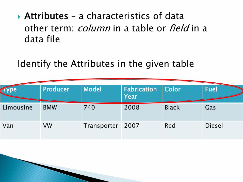
Attributes – a characteristics of data

other term: column in a table or field in a data file

Identify the Attributes in the given table

Type Producer Model Fabrication Year

Color Fuel

Limousine BMW 740 2008 Black Gas

Van VW Transporter 2007 Red Diesel

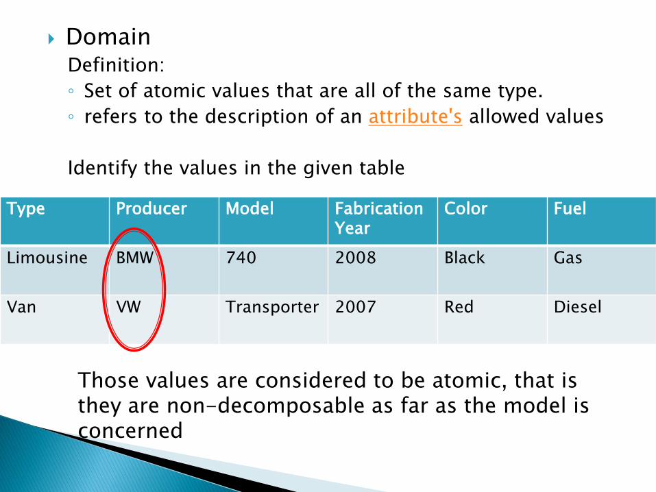
Domain Definition:

◦ Set of atomic values that are all of the same type.

◦ refers to the description of an attribute's allowed values

Identify the values in the given table

Type Producer Model Fabrication

Year Color Fuel

Limousine BMW 740 2008 Black Gas

Van VW Transporter 2007 Red Diesel

Those values are considered to be atomic, that is they are non-decomposable as far as the model is concerned

Domain

Name – use for references

Dimension - given by the number of values that domain has

◦ A given attribute may have the same name as the corresponding domain, but this situation should be avoided because it can generate confusion

Tuples

Definition

an ordered set of values that describe data characteristics at one moment in time

Also called as n-tuple

Identify the tuple in given table

There are informal term used for a tuple: the row in a table or record in a data file.

Type Producer Model Fabrication Year

Color Fuel

Limousine BMW 740 2008 Black Gas

Van VW Transporter 2007 Red Diesel

Relation ◦ the core of the relational data

◦ A relation consist of the Heading and the Body

Heading consists of a fixed set of attributes, each attribute Ai corresponds to exactly one of the underlying domains Di

Body consists of a time-varying set of tuples, where each tuple in turn consists of a set of attribute-value pairs (Ai:vi) : vi is a value from the unique domain Di that is associated with the attribute Ai.

Type Producer

Model Fabrication Year

Color Fuel

Limousine

BMW 740 2008 Black Gas

Van VW Transporter

2007 Red Diesel

Heading

Body

A relation degree is equivalent with the number of attributes of that relation.

◦ A relation of degree one is called unary,

◦ A relation of degree two is binary

◦ a relation of degree three is ternary, and so on.

◦ A relation of degree n is called nary.

How many relation degree has the given illustration?

Relation cardinality is equivalent with the number of tuples of that relation. The cardinality of a relation changes with time, whereas the degree does not change that often.

the body consists of a time-varying set of tuples. At one moment in time, the relation cardinality may be m, while another moment in time the same relation may have the cardinality n. The state in which a relation exists at one moment in time is called a relation instance. Therefore, during a relation’s lifetime there may be many relation instances

Four properties posses by relation ◦ There are no duplicate tuples in a relation ◦ Tuples are unordered (top to bottom) ◦ Attributes are unordered (left to right) ◦ All attribute values are atomic

Schemas ◦ database schema is a formal description of all the

database relations and all the relationships existing between them (Will discuss with conceptual data modeling)

Keys ◦ The relational data model uses keys to define

identifiers for a relation’s tuples. The keys are used to enforce rules and/or constraints on database data. Those constraints are essential for maintaining data consistency and correctness

3 different type of Keys

◦ Candidate Key

◦ Foreign Key

◦ Primary Key

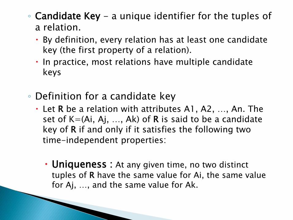
◦ Candidate Key - a unique identifier for the tuples of a relation.

By definition, every relation has at least one candidate key (the first property of a relation).

In practice, most relations have multiple candidate keys

◦ Definition for a candidate key

Let R be a relation with attributes A1, A2, …, An. The set of K=(Ai, Aj, …, Ak) of R is said to be a candidate key of R if and only if it satisfies the following two

time-independent properties:

Uniqueness : At any given time, no two distinct

tuples of R have the same value for Ai, the same value for Aj, …, and the same value for Ak.

Minimality None of Ai, Aj, …, Ak can be discarded from K

without destroying the uniqueness property.

◦ A candidate key is sometimes called a unique key . A unique key can be specified at the Data Definition Language (DDL) level using the UNIQUE parameter beside the attribute name. If a relation has more than one candidate key, the one that is chosen to represent the relation is called the primary key, and the remaining candidate keys are called alternate keys.

◦ Every relation has at least one candidate key, because at least the combination of all of its attributes has the uniqueness property (the first property of a relation), but usually exist at least one other candidate key made of fewer attributes of the relation.

Primary key ◦ is a unique identifier of the relation tuples

◦ it is a candidate key that is chosen to represent the relation in the database and to provide a way to uniquely identify each tuple of the relation.

◦ Relational DBMS allow a primary key to be specified the moment you create the relation (table)

◦ For a candidate key to be chosen as primary key this attribute values must be “UNIQUE” and “NOT NULL” for all tuples from all relation instances.

There are situations when real-world characteristic of data, modeled by that relation, do not have unique values. In this case, the primary key must be the combination of all relation attributes.

Such a primary key is not a convenient one for practical matters as it would require too much physical space for storage, and maintaining relationships between database relations would be more difficult. In those cases, the solution adopted is to introduce another attribute, like an ID, with no meaning to real-world data, which will have unique values and will be used as a primary key. This attribute is usually called a surrogate key. Sometimes, in database literature, you will also find it referenced as artificial key.

Foreign keys ◦ is an attribute (or attribute combination) in one relation R2

whose values are required to match those of the primary key of some relation R1 (R1 and R2 not necessarily distinct). Note that a foreign key and the corresponding primary key should be defined on the same underlying domain.

Foreign-to-primary-key matches represent references from one relation to another. They are the “glue” that holds the database together. Another way of saying this is that foreign-to-primary-key matches represent certain relationships between tuples. Note carefully, however, that not all such relationships are represented by foreign-to-primary-key matches.

The DDL sublanguage usually has a FOREIGN KEY construct for defining the foreign keys. For each foreign key the corresponding primary key and its relation is also specified.

DEFINE

data integrity can be achieved using integrity rules or constraints to ensure that the overall result is still in a correct state.

Entity integrity constraint ◦ no attribute participating in the primary key of a

relation is allowed to accept null values

◦ null represents property inapplicable or information unknown

indicates the absence of a value, an undefined value

Justification ◦ Database relations correspond to entities from the

real-world and they are distinguishable, they have a unique identification of some kind

◦ Primary keys perform the unique identification function in the relational model

◦ null primary key value would be a contradiction in terms because it would be saying that there is some entity that has no identity that does not exist.

Referential integrity constraint ◦ if a relation R2 includes a foreign key ◦ every value of FK in R2 must either be equal to the value

of PK in some tuple of R1 or be wholly null (each attribute value participating in that FK value must be null). R1 and R2 are not necessarily distinct.

◦ Justification If some tuple t2 from relation R2 references some tuple t1

from relation R1, then tuple t1 must exist, otherwise it does not make sense

a given foreign key value must have a matching primary key value

Sometimes, for practical reasons, it is necessary to permit the foreign key to accept null values

Referential Integrity ◦ For example:

OWNERS relation the foreign key is identificationNumber. This attribute value must have matching values in the CARS relation, because a person must own an existing car to become an owner. If the foreign key has a null value, that means that the person does not yet have a car, but he could buy an existing one.

Semantic integrity constraints ◦ refers to the correctness of the meaning of the data

◦ a predicate that all correct states of relations instances from the database are required to satisfy.

◦ For example:

the street number attribute value from the OWNERS relation must be positive, because the real-world street numbers are positive.

Domain constraint ◦ states that values of the attribute in question are

required to belong to the set on values constituting the underlying domain.

◦ For example:

the Street attribute domain of OWNERS relation is CHAR(20), because streets have names in general and Number attribute domain is NUMERIC, because street numbers are numeric values.

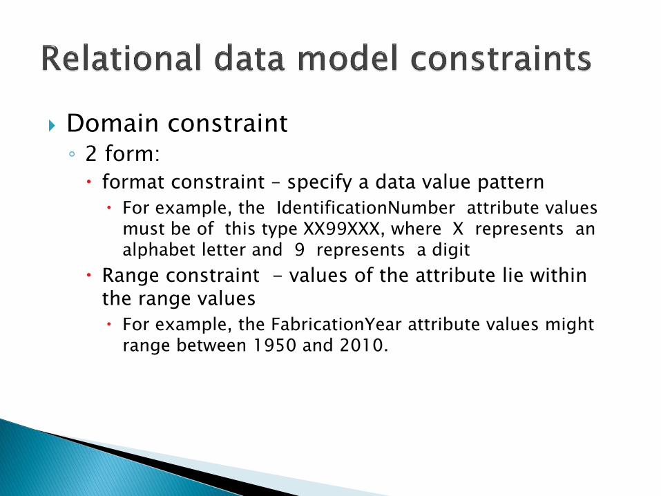
Domain constraint ◦ 2 form:

format constraint – specify a data value pattern

For example, the IdentificationNumber attribute values must be of this type XX99XXX, where X represents an alphabet letter and 9 represents a digit

Range constraint - values of the attribute lie within the range values

For example, the FabricationYear attribute values might range between 1950 and 2010.

Null constraint ◦ attribute values cannot be null. from every relation

instance, that attribute must have a value which exists in the underlying attribute domain

◦ For example, FirstName and LastName attributes values cannot be null, this means that a car owner must have a name.

◦ specified with the NOT NULL construct and The attribute name is followed by the words NOT NULL for that

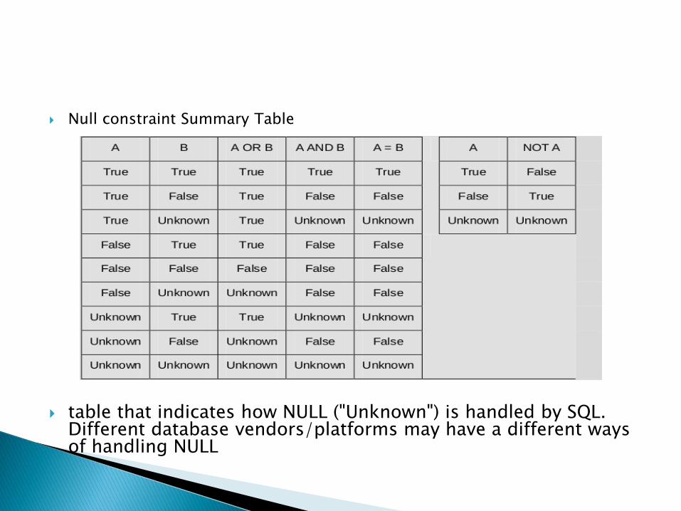
Null constraint Summary Table

table that indicates how NULL ("Unknown") is handled by SQL. Different database vendors/platforms may have a different ways of handling NULL

Unique constraint ◦ attribute values must be different

◦ For example, in the CARS relation the SerialNumber attribute values must be unique, because it is not possible to have two cars and only one engine

◦ A unique constraint is usually specified with an attribute name followed by the word UNIQUE. Note that NULL is a valid unique value

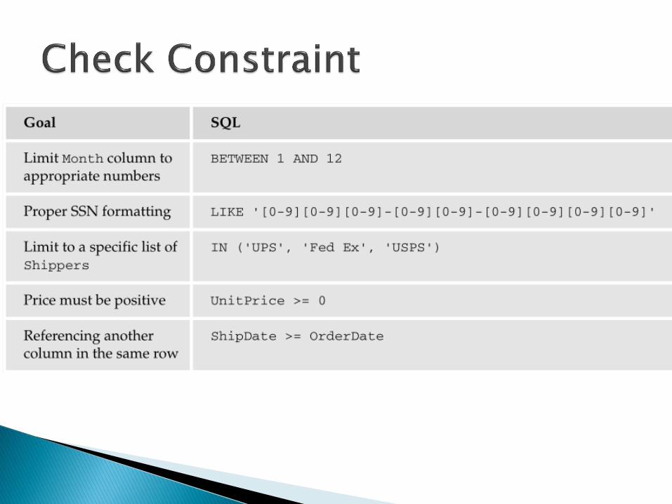
Check constraint ◦ specifies a condition on a relation data, which is always

checked when data is manipulated

predicate states what to check, and optionally what to do if the check fails

◦ When the constraint is executed, the system checks to see whether the current state of the database satisfies the specified constraint. If it does not, the constraint is rejected, otherwise it is accepted and enforced from that time on.

◦ For example, an employee's salary can’t be greater than his manager's salary or a department manager can’t have more that 20 people reporting to him.

a set of operators to manipulate relations

Group ◦ The traditional set operations: union, intersection,

difference and Cartesian product

◦ The special relational operations: select, project, join and divide.

Union U ◦ is the set of all tuples t belonging to either R1 or R2

or both.

◦ Two relations are union-compatible if they have the same degree, and the ith attribute of each is based on the same domain.

◦ UNION operation is associative and commutative

Figure 2.5 provides an example of a UNION operation. The operands are relation R1 and relation R2 and the result is another relation R3 with 5 tuples.

Intersection ∩ ◦ R1 INTERSECT R2, is the set of all tuples t belonging

to both R1 and R2.

◦ INTERSECT operation is associative and commutative.

◦ Figure 2.6 provides an example of an INTERSECT operation. The operands are relation R1 and relation R2 and the result is another relation R3 with only one tuple

Figure 2.6 provides an example of an INTERSECT operation. The operands are relation R1 and relation R2 and the result is another relation R3 with only one tuple

Difference - ◦ R1 MINUS R2 is the set of all tuples t belonging to

R1 and not to R2

◦ DIFFERENCE operation is not associative and commutative.

◦ Figure 2.7 provides an example of a DIFFERECE operation. The operands are relation R1 and relation R2 and the result is another relation R3 with two tuples. As you can see, the result of R1-R2 is different from R2-R1.

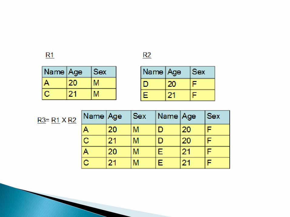
Cartesian product x ◦ R1 TIMES R2, is the set of all tuples t such that t

is the concatenation of a tuple r belonging to R1 and a tuple s belonging to R2

◦ R1 and R2 don’t have to be union-compatible.

◦ If R1 has degree n and cardinality N1 and R2 has degree m and cardinality N2 then the resulting relation R3 has degree (n+m) and cardinality (N1*N2). This is illustrated in Figure 2.8.

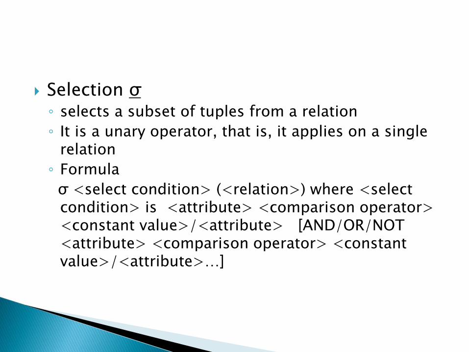
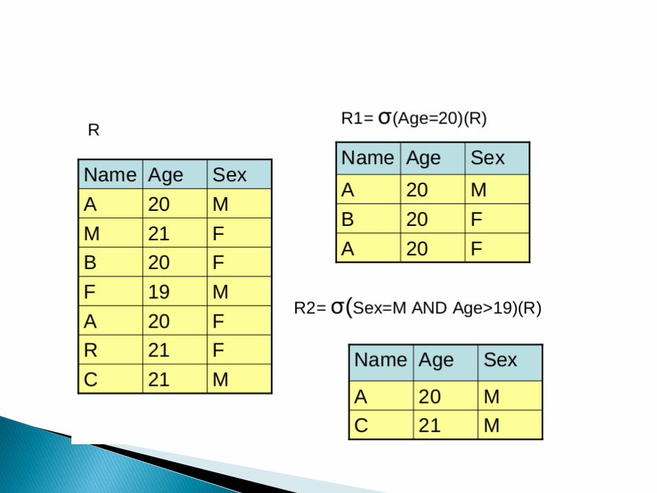
Selection σ ◦ selects a subset of tuples from a relation

◦ It is a unary operator, that is, it applies on a single relation

◦ Formula

σ <select condition> (<relation>) where <select condition> is <attribute> <comparison operator> <constant value>/<attribute> [AND/OR/NOT <attribute> <comparison operator> <constant value>/<attribute>…]

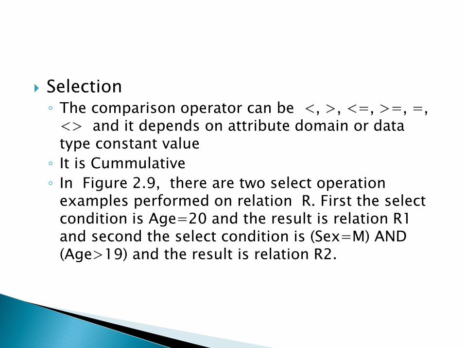
Selection ◦ The comparison operator can be <, >, <=, >=, =,

<> and it depends on attribute domain or data type constant value

◦ It is Cummulative

◦ In Figure 2.9, there are two select operation examples performed on relation R. First the select condition is Age=20 and the result is relation R1 and second the select condition is (Sex=M) AND (Age>19) and the result is relation R2.

Projection π ◦ builds another relation by selecting a subset of

attributes of an existing relation

◦ Duplicate tuples from the resulting relation are eliminated. It is also a unary operator

◦ Formula

π<attribute list> (<relation>) where <attribute list>

◦ The result relation degree is equal with the number of attributes from <attribute list> because only those attributes will appear

In Figure 2.10 there are two project operation examples performed on relation R. First the projection is made on attributes Name and Sex and the result is relation R1 and second the projection is made on attributes Age and Sex and the result is relation R2.

project_{beer} ( ((\project_{name} // all drinkers Drinker)

\diff (\rename_{name} // rename so we can diff \project_{drinker} // drinkers who frequent JJP

\select_{bar = 'James Joyce Pub'} Frequents)) \join_{drinker = name} /* join with Likes to find beers */

Join ►◄ ◦ concatenates two relations based on a joining

condition or predicate. It must have at least one common attribute with the same underlying domain to specify a joining condition

◦ Formula where <join condition> is <attribute from R>

<comparison operator> < <attribute from S>

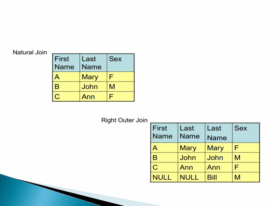
In Figure 2.11 there are two relations R1 and R2 joined on a join condition where LastName from relation R1 is equal with LastName from relation R2. The resulting relation is R3.

Type of join ◦ theta-join – the result of a join must include two

identical attributes from the point of view of their values

If the result is another relation T that contains all the tuples t such that t is the concatenation of a tuple r belonging to R and a tuple s belonging to S if the join condition is true

natural join - one of two attributes is eliminated

Equijoin - most often used, It means that the comparison operator is =.

Type of join ◦ outer join

when not all the tuples from relation R have a corresponding tuple in relation S. The tuples won’t appear in the result of a join operation between R and S. In this case it is necessary to have all tuples in the result

3 forms of outer join

left outer join - where all tuples from R will be in the result

right outer join - where all tuples from S will be in the Result

full outer join - all tuples from R and S will be in the result

Figure 2.11 there are two relations R1 and R2 joined on a join condition where LastName from relation R1 is equal with LastName from relation R2. The resulting relation is R3

Division ÷ ◦ The division operator divides a relation R1 of

degree (n+m) by a relation R2 of degree m and produces a relation of degree n

◦ The result between R1 and R2 is another relation, which contains all the tuples that concatenated with all R2 tuples are belonging to R1 relation.

◦ Figure 2.13 provides an example of a division operation between relation R1 and R2.

represents an alternative to relational algebra as a candidate for the manipulative part of the relational data model

Difference ◦ Algebra provides a collection of explicit operations

that can be actually used to build some desired relation from the given relations in the database.

◦ Calculus provides a notation for formulating the definition of that desired relation in terms of those given relations

Example

Consider the query “Get owners’ complete names and cities for owners who own a red car.” ◦ algebraic version

Join relation OWNERS with relation CARS on IdentificationNumber attributes

Select from the resulting relation only those tuples with car Colour = ”RED”

Project the result of that restriction on owner FirstName, LastName and City

◦ calculus formulation

Get FirstName, LastName and City for cars owners such that there exists a car with the same IdentificationNumber and with RED color.

◦ Two types of relational calculus:

Tuple-oriented relational calculus – based on tuple variable concept

Domain-oriented relational calculus – based on domain variable concept

Tuple-oriented relational calculus ◦ A tuple variable is a variable that ranges over some

relation. A variable whose only permitted values are tuples of that relation

◦ if tuple variable T ranges over relation R, then, at any given time, T represents some tuple t of R.

◦ Example, the query “Get FirstName, LastName and City for cars owners such that there exists a car with the same identificationNumber and with RED color” can be expressed as follows: RANGE OF OWNERS IS OWNERS.FirstName,

OWNERS.LastName, OWNERS.City WHERE ∃ CARS(CARS.IdentificationNumber=OWNERS.IdentificationNumber AND CARS.Color=’RED’)

◦ The tuple calculus is formally equivalent to the relational algebra.

◦ The QUEL language from INGRES is based on tuple-oriented relational calculus.

Domain-oriented relational calculus ◦ tuple variables are replaced by domain variables.

A domain variable is a variable that ranges over a domain instead of a relation

◦ Each occurrence of a domain variable can be also free or bound. A bound domain variable occurs as the variable immediately following one of the quantifiers: the existential quantifier ∃ or the universal quantifier ∀. In all other cases, the variable is called a free variable.

For example, the query “Get FirstName, LastName and City for cars owners such that there exists a car with the same IdentificationNumber and with RED color” can be expressed as follows: ◦ FirstNameX, LastNameX, CityX WHERE ∃

IdentificationNumberX (OWNERS (IdentificationNumber:IdentificationNumberX,

◦ FirstName:FirstNameX, LastName:LastNameX, City:CityX) AND CARS(IdentificationNumber:IdentificationNumberX, Color:’RED’)