![i .] APPROXIMATING HARMONIC FUNCTIONS 499€¦ · APPROXIMATING HARMONIC FUNCTIONS 499 THE APPROXIMATION OF HARMONIC FUNCTIONS BY HARMONIC POLYNOMIALS AND BY HARMONIC RATIONAL FUNCTIONS*](https://static.fdocuments.us/doc/165x107/5f0873ba7e708231d42214c2/i-approximating-harmonic-functions-499-approximating-harmonic-functions-499-the.jpg)
Introduction to Harmonic Analysis - Peoplepeople.math.gatech.edu/~heil/handouts/chap1.pdf ·...
93
Christopher Heil Introduction to Harmonic Analysis November 12, 2010 Springer Berlin Heidelberg NewYork Hong Kong London Milan Paris Tokyo
Transcript of Introduction to Harmonic Analysis - Peoplepeople.math.gatech.edu/~heil/handouts/chap1.pdf ·...
Christopher Heil
Introduction to Harmonic
Analysis
November 12, 2010
Springer
Berlin Heidelberg NewYork
HongKong London
Milan Paris Tokyo

Contents
General Notation . . . . . . . . . . . . . . . . . . . . . . . . . . . . . . . . . . . . . . . . . . . . . . xi
1 The Fourier Transform on L1(R) . . . . . . . . . . . . . . . . . . . . . . . . . . . 1
1.1 Definition and Basic Properties . . . . . . . . . . . . . . . . . . . . . . . . . . . 11.1.1 The Fourier Transform on L1(R) . . . . . . . . . . . . . . . . . . . . 11.1.2 Motivation . . . . . . . . . . . . . . . . . . . . . . . . . . . . . . . . . . . . . . . 5
1.2 Translation, Modulation, Dilation, and Involution . . . . . . . . . . . 101.2.1 Four Fundamental Operators . . . . . . . . . . . . . . . . . . . . . . . 111.2.2 The Riemann–Lebesgue Lemma . . . . . . . . . . . . . . . . . . . . . 131.2.3 Position and Momentum . . . . . . . . . . . . . . . . . . . . . . . . . . . 141.2.4 The HRT Conjecture . . . . . . . . . . . . . . . . . . . . . . . . . . . . . . 15
1.3 Convolution . . . . . . . . . . . . . . . . . . . . . . . . . . . . . . . . . . . . . . . . . . . . 161.3.1 Some Notational Conventions . . . . . . . . . . . . . . . . . . . . . . . 171.3.2 Definition and Basic Properties of Convolution . . . . . . . . 181.3.3 Young’s Inequality . . . . . . . . . . . . . . . . . . . . . . . . . . . . . . . . . 201.3.4 Convolution as Filtering; Lack of an Identity . . . . . . . . . . 211.3.5 Convolution as Averaging; Introduction to
Approximate Identities . . . . . . . . . . . . . . . . . . . . . . . . . . . . . 221.3.6 Convolution as an Inner Product . . . . . . . . . . . . . . . . . . . . 251.3.7 Convolution and Smoothing . . . . . . . . . . . . . . . . . . . . . . . . 261.3.8 Convolution and Differentiation . . . . . . . . . . . . . . . . . . . . . 281.3.9 Convolution and Banach Algebras . . . . . . . . . . . . . . . . . . . 291.3.10 Convolution on General Domains . . . . . . . . . . . . . . . . . . . . 32
1.4 The Duality Between Smoothness and Decay . . . . . . . . . . . . . . . . 361.4.1 Decay in Time Implies Smoothness in Frequency . . . . . . 361.4.2 A Primer on Absolute Continuity . . . . . . . . . . . . . . . . . . . . 381.4.3 Smoothness in Time Implies Decay in Frequency . . . . . . 411.4.4 The Riemann–Lebesgue Lemma Revisited . . . . . . . . . . . . 42
1.5 Approximate Identities . . . . . . . . . . . . . . . . . . . . . . . . . . . . . . . . . . . 461.5.1 Definition and Existence of Approximate Identities . . . . 461.5.2 Approximation in Lp(R) by an Approximate Identity . . 48

vi Contents
1.5.3 Uniform Convergence . . . . . . . . . . . . . . . . . . . . . . . . . . . . . . 521.5.4 Pointwise Convergence . . . . . . . . . . . . . . . . . . . . . . . . . . . . . 531.5.5 Dense Sets of Nice Functions . . . . . . . . . . . . . . . . . . . . . . . . 541.5.6 The C∞ Urysohn Lemma . . . . . . . . . . . . . . . . . . . . . . . . . . 551.5.7 Gibbs’s Phenomenon. . . . . . . . . . . . . . . . . . . . . . . . . . . . . . . 561.5.8 Translation-Invariant Subspaces of L1(R) . . . . . . . . . . . . . 57
1.6 The Inversion Formula . . . . . . . . . . . . . . . . . . . . . . . . . . . . . . . . . . . 601.6.1 The Fejer Kernel . . . . . . . . . . . . . . . . . . . . . . . . . . . . . . . . . . 601.6.2 Proof of the Inversion Formula . . . . . . . . . . . . . . . . . . . . . . 621.6.3 Summability . . . . . . . . . . . . . . . . . . . . . . . . . . . . . . . . . . . . . . 651.6.4 Pointwise Inversion . . . . . . . . . . . . . . . . . . . . . . . . . . . . . . . . 671.6.5 Decay and Smoothness Revisited . . . . . . . . . . . . . . . . . . . . 69
1.7 The Range of the Fourier Transform . . . . . . . . . . . . . . . . . . . . . . . 721.8 Some Special Kernels . . . . . . . . . . . . . . . . . . . . . . . . . . . . . . . . . . . . 741.9 The Schwartz Space . . . . . . . . . . . . . . . . . . . . . . . . . . . . . . . . . . . . . 79
1.9.1 Definition and Basic Properties . . . . . . . . . . . . . . . . . . . . . 801.9.2 Topology and Convergence in the Schwartz Space . . . . . 801.9.3 Invariance of the Schwartz Space . . . . . . . . . . . . . . . . . . . . 81
2 Fourier Series and the Abstract Fourier Transform . . . . . . . . 852.1 The Abstract Fourier Transform . . . . . . . . . . . . . . . . . . . . . . . . . . . 85
2.1.1 Examples of Locally Compact Abelian Groups . . . . . . . . 852.1.2 Characters and the Fourier Transform . . . . . . . . . . . . . . . 872.1.3 The Fourier Transform on LCA Groups . . . . . . . . . . . . . . 90
2.2 Fourier Series and Approximate Identities on the Torus . . . . . . 922.2.1 Partial Sums and the Dirichlet and Fejer Kernels . . . . . . 962.2.2 Approximate Identities . . . . . . . . . . . . . . . . . . . . . . . . . . . . . 992.2.3 Cesaro Summability and the Inversion Formula . . . . . . . 101
2.3 Completeness and the L2-Theory . . . . . . . . . . . . . . . . . . . . . . . . . . 1062.3.1 Completeness . . . . . . . . . . . . . . . . . . . . . . . . . . . . . . . . . . . . . 1062.3.2 The L2 Theory . . . . . . . . . . . . . . . . . . . . . . . . . . . . . . . . . . . . 1072.3.3 Minimality . . . . . . . . . . . . . . . . . . . . . . . . . . . . . . . . . . . . . . . 108
2.4 Weyl’s Equidistribution Theorem . . . . . . . . . . . . . . . . . . . . . . . . . . 1122.5 Basis Properties of the Trignometric System . . . . . . . . . . . . . . . . 115
2.5.1 Schauder Bases and the Partial Sum Operators . . . . . . . 1162.5.2 The Symmetric Partial Sum Operators and Their
Relatives . . . . . . . . . . . . . . . . . . . . . . . . . . . . . . . . . . . . . . . . . 1182.6 The Conjugate Function and Norm Convergence of Fourier
Series . . . . . . . . . . . . . . . . . . . . . . . . . . . . . . . . . . . . . . . . . . . . . . . . . . 1222.7 Pointwise Convergence . . . . . . . . . . . . . . . . . . . . . . . . . . . . . . . . . . . 1272.8 The Poisson Summation Formula . . . . . . . . . . . . . . . . . . . . . . . . . . 1362.9 Wiener’s Lemma . . . . . . . . . . . . . . . . . . . . . . . . . . . . . . . . . . . . . . . . 1382.10 Wiener’s Tauberian Theorem . . . . . . . . . . . . . . . . . . . . . . . . . . . . . 1412.11 Ideals . . . . . . . . . . . . . . . . . . . . . . . . . . . . . . . . . . . . . . . . . . . . . . . . . . 144
Contents vii
3 The Fourier Transform on L2(R) . . . . . . . . . . . . . . . . . . . . . . . . . . . 149
3.1 Definition and Basic Properties of the Fourier Transform onL2(R) . . . . . . . . . . . . . . . . . . . . . . . . . . . . . . . . . . . . . . . . . . . . . . . . . . 149
3.2 The Hermite Functions . . . . . . . . . . . . . . . . . . . . . . . . . . . . . . . . . . . 1563.2.1 Construction of the Hermite Functions . . . . . . . . . . . . . . . 1563.2.2 Wiener’s Definition of the Fourier Transform on L2(R) . 159
3.3 The Fourier Transform on Lp(R) . . . . . . . . . . . . . . . . . . . . . . . . . . 1613.4 The Classical Uncertainty Principle . . . . . . . . . . . . . . . . . . . . . . . . 165
3.4.1 Concentration and the Statement of the ClassicalUncertainty Principle . . . . . . . . . . . . . . . . . . . . . . . . . . . . . . 165
3.4.2 Simultaneous Approximation and Smoothness versusDecay . . . . . . . . . . . . . . . . . . . . . . . . . . . . . . . . . . . . . . . . . . . . 168
3.4.3 Proof of the Classical Uncertainty Principle . . . . . . . . . . . 1713.4.4 Additive Form of the Uncertainty Principle . . . . . . . . . . . 1723.4.5 Operator-Theoretic Proof of the Uncertainty Principle . 1743.4.6 Hermite Function Proof of the Uncertainty Principle . . . 1743.4.7 A Local Uncertainty Principle . . . . . . . . . . . . . . . . . . . . . . 175
3.5 The Paley–Wiener Theorem . . . . . . . . . . . . . . . . . . . . . . . . . . . . . . 1763.5.1 Motivation . . . . . . . . . . . . . . . . . . . . . . . . . . . . . . . . . . . . . . . 177
3.6 A Primer on Hilbert–Schmidt Operators . . . . . . . . . . . . . . . . . . . . 1823.7 The Donoho–Stark Uncertainty Principle . . . . . . . . . . . . . . . . . . . 183
3.7.1 Concentration and Essential Support . . . . . . . . . . . . . . . . 1843.7.2 Products of Time- and Frequency-Limiting Operators . . 1853.7.3 The Donoho–Stark Uncertainty Principle . . . . . . . . . . . . . 1863.7.4 Size of the Supports . . . . . . . . . . . . . . . . . . . . . . . . . . . . . . . 187
3.8 Energy Concentration . . . . . . . . . . . . . . . . . . . . . . . . . . . . . . . . . . . . 1893.8.1 Time-Frequency Limiting Operators . . . . . . . . . . . . . . . . . 1893.8.2 Restatement of the Problem . . . . . . . . . . . . . . . . . . . . . . . . 1913.8.3 Time-Frequency Limiting Operators and the Spectral
Theorem . . . . . . . . . . . . . . . . . . . . . . . . . . . . . . . . . . . . . . . . . 1923.8.4 Double Orthogonality . . . . . . . . . . . . . . . . . . . . . . . . . . . . . . 1933.8.5 Prolate Spheroidal Wave Functions . . . . . . . . . . . . . . . . . . 1943.8.6 Behavior of the Eigenvalues . . . . . . . . . . . . . . . . . . . . . . . . . 1953.8.7 The Space of Band- and Time-Limited Functions . . . . . . 1973.8.8 The Range of Time-Frequency Concentrations . . . . . . . . 199
4 Distributions . . . . . . . . . . . . . . . . . . . . . . . . . . . . . . . . . . . . . . . . . . . . . . 2054.1 Motivation and Notation . . . . . . . . . . . . . . . . . . . . . . . . . . . . . . . . . 206
4.1.1 Notation for Functionals . . . . . . . . . . . . . . . . . . . . . . . . . . . 2074.2 Convergence and Continuity . . . . . . . . . . . . . . . . . . . . . . . . . . . . . . 209
4.2.1 Examples of Spaces Defined by Seminorms . . . . . . . . . . . 2094.2.2 Convergence . . . . . . . . . . . . . . . . . . . . . . . . . . . . . . . . . . . . . . 2124.2.3 From Convergence to a Metric . . . . . . . . . . . . . . . . . . . . . . 2134.2.4 Continuity Equals Boundedness . . . . . . . . . . . . . . . . . . . . . 214
4.3 Distributions of Various Sorts . . . . . . . . . . . . . . . . . . . . . . . . . . . . . 216
viii Contents
4.3.1 The Schwartz Class and the Space of TemperedDistributions . . . . . . . . . . . . . . . . . . . . . . . . . . . . . . . . . . . . . 216
4.3.2 C∞(R) and the Space of Compactly SupportedDistributions . . . . . . . . . . . . . . . . . . . . . . . . . . . . . . . . . . . . . 218
4.3.3 Convergence in C∞c (R) . . . . . . . . . . . . . . . . . . . . . . . . . . . . . 219
4.3.4 The Space of Distributions . . . . . . . . . . . . . . . . . . . . . . . . . 2204.3.5 Inclusions . . . . . . . . . . . . . . . . . . . . . . . . . . . . . . . . . . . . . . . . 2234.3.6 Convergence of Distributions . . . . . . . . . . . . . . . . . . . . . . . . 224
4.4 Functions as Distributions . . . . . . . . . . . . . . . . . . . . . . . . . . . . . . . . 2274.4.1 Locally Integrable Functions . . . . . . . . . . . . . . . . . . . . . . . . 2284.4.2 Functions with Polynomial Growth . . . . . . . . . . . . . . . . . . 2304.4.3 Compactly Supported Functions . . . . . . . . . . . . . . . . . . . . . 232
4.5 Operations on Distributions . . . . . . . . . . . . . . . . . . . . . . . . . . . . . . 2334.5.1 Translation, Modulation, Dilation, Conjugation, and
Involution . . . . . . . . . . . . . . . . . . . . . . . . . . . . . . . . . . . . . . . . 2334.5.2 Products of Distributions with Smooth Functions . . . . . . 2364.5.3 Convolution of Distributions with Smooth Functions . . . 2364.5.4 Convolution and Translation-Invariant Operators . . . . . . 241
4.6 Support . . . . . . . . . . . . . . . . . . . . . . . . . . . . . . . . . . . . . . . . . . . . . . . . 2444.6.1 Definition and Basic Properties . . . . . . . . . . . . . . . . . . . . . 2444.6.2 Compactly Supported Distributions . . . . . . . . . . . . . . . . . . 2464.6.3 Convolution of Distributions . . . . . . . . . . . . . . . . . . . . . . . . 248
4.7 Differentiation . . . . . . . . . . . . . . . . . . . . . . . . . . . . . . . . . . . . . . . . . . 2494.7.1 Definition and Basic Properties . . . . . . . . . . . . . . . . . . . . . 2494.7.2 A Relation between Classical and Distributional
Differentiation . . . . . . . . . . . . . . . . . . . . . . . . . . . . . . . . . . . . 2514.7.3 Distributions and Derivatives of Continuous Functions . 2554.7.4 Distributions Supported at a Point . . . . . . . . . . . . . . . . . . 256
4.8 The Fourier Transform of Tempered Distributions . . . . . . . . . . . 2594.8.1 Definition of the Distributional Fourier Transform . . . . . 2604.8.2 Basic Properties of the Fourier Transform . . . . . . . . . . . . 2614.8.3 The Paley–Wiener Theorem for Tempered Distributions 2624.8.4 The Distributional Poisson Summation Formula . . . . . . . 2644.8.5 The Hilbert Transform . . . . . . . . . . . . . . . . . . . . . . . . . . . . . 265
4.9 Sobolev Spaces . . . . . . . . . . . . . . . . . . . . . . . . . . . . . . . . . . . . . . . . . . 2704.9.1 Definition and Basic Properties . . . . . . . . . . . . . . . . . . . . . 2704.9.2 Sobolev Spaces and Distributional Derivatives . . . . . . . . . 2724.9.3 Duality . . . . . . . . . . . . . . . . . . . . . . . . . . . . . . . . . . . . . . . . . . 2734.9.4 The Sobolev Embedding Theorem . . . . . . . . . . . . . . . . . . . 274
5 Measures . . . . . . . . . . . . . . . . . . . . . . . . . . . . . . . . . . . . . . . . . . . . . . . . . . 2775.1 Borel and Radon Measures on R . . . . . . . . . . . . . . . . . . . . . . . . . . 277
5.1.1 Convolution and Linear Time-Invariant Systems . . . . . . . 277

Contents ix
A Lebesgue Measure and Integration . . . . . . . . . . . . . . . . . . . . . . . . . 281A.1 Exterior Lebesgue Measure . . . . . . . . . . . . . . . . . . . . . . . . . . . . . . . 281A.2 Lebesgue Measure . . . . . . . . . . . . . . . . . . . . . . . . . . . . . . . . . . . . . . . 282A.3 Measurable Functions . . . . . . . . . . . . . . . . . . . . . . . . . . . . . . . . . . . . 284A.4 The Lebesgue Integral . . . . . . . . . . . . . . . . . . . . . . . . . . . . . . . . . . . 286A.5 The Dominated Convergence Theorem . . . . . . . . . . . . . . . . . . . . . 289A.6 The Lebesgue Differentiation Theorem . . . . . . . . . . . . . . . . . . . . . 290A.7 Repeated Integration . . . . . . . . . . . . . . . . . . . . . . . . . . . . . . . . . . . . 290
B Spaces and Operators . . . . . . . . . . . . . . . . . . . . . . . . . . . . . . . . . . . . . . 293B.1 Metrics and Convergence . . . . . . . . . . . . . . . . . . . . . . . . . . . . . . . . . 293B.2 Norms and Seminorms . . . . . . . . . . . . . . . . . . . . . . . . . . . . . . . . . . . 294B.3 Examples of Banach Spaces . . . . . . . . . . . . . . . . . . . . . . . . . . . . . . . 296
B.3.1 The ℓp Spaces . . . . . . . . . . . . . . . . . . . . . . . . . . . . . . . . . . . . . 296B.3.2 More Sequence Spaces . . . . . . . . . . . . . . . . . . . . . . . . . . . . . 297B.3.3 The Lp spaces . . . . . . . . . . . . . . . . . . . . . . . . . . . . . . . . . . . . 298B.3.4 Some Spaces of Continuous Functions . . . . . . . . . . . . . . . . 300
B.4 Inner Products . . . . . . . . . . . . . . . . . . . . . . . . . . . . . . . . . . . . . . . . . . 301B.5 Orthogonality . . . . . . . . . . . . . . . . . . . . . . . . . . . . . . . . . . . . . . . . . . . 303B.6 Linear Operators on Normed Spaces . . . . . . . . . . . . . . . . . . . . . . . 304
B.6.1 Equivalence of Boundedness and Continuity . . . . . . . . . . 305B.6.2 Isometries and Isomorphisms . . . . . . . . . . . . . . . . . . . . . . . 306B.6.3 Orthogonal Projections . . . . . . . . . . . . . . . . . . . . . . . . . . . . 307B.6.4 The Space B(X, Y ) . . . . . . . . . . . . . . . . . . . . . . . . . . . . . . . . 307
B.7 The Dual of a Hilbert Space and Notation for Functionals . . . . 308B.8 The Dual of Lp(E) . . . . . . . . . . . . . . . . . . . . . . . . . . . . . . . . . . . . . . 309B.9 Adjoints for Operators on Hilbert Spaces . . . . . . . . . . . . . . . . . . . 310B.10 Self-Adjoint Operators . . . . . . . . . . . . . . . . . . . . . . . . . . . . . . . . . . . 311
C Functional Analysis on Banach Spaces . . . . . . . . . . . . . . . . . . . . . 313C.1 The Hahn–Banach Theorem . . . . . . . . . . . . . . . . . . . . . . . . . . . . . . 313C.2 Reflexivity . . . . . . . . . . . . . . . . . . . . . . . . . . . . . . . . . . . . . . . . . . . . . . 315C.3 Adjoints of Operators on Banach Spaces . . . . . . . . . . . . . . . . . . . . 316C.4 The Baire Category Theorem . . . . . . . . . . . . . . . . . . . . . . . . . . . . . 317C.5 The Uniform Boundedness Principle . . . . . . . . . . . . . . . . . . . . . . . 318C.6 The Open Mapping Theorem . . . . . . . . . . . . . . . . . . . . . . . . . . . . . 319C.7 The Closed Graph Theorem . . . . . . . . . . . . . . . . . . . . . . . . . . . . . . 321C.8 Weak and Weak* Convergence . . . . . . . . . . . . . . . . . . . . . . . . . . . . 321
D Convergence, Completeness, and Schauder Bases . . . . . . . . . . 323D.1 Convergent Series . . . . . . . . . . . . . . . . . . . . . . . . . . . . . . . . . . . . . . . 323D.2 Unconditional Convergence . . . . . . . . . . . . . . . . . . . . . . . . . . . . . . . 324D.3 Span and Closed Span . . . . . . . . . . . . . . . . . . . . . . . . . . . . . . . . . . . 327D.4 Orthonormal Sequences in Hilbert Spaces . . . . . . . . . . . . . . . . . . . 328D.5 Hamel Bases . . . . . . . . . . . . . . . . . . . . . . . . . . . . . . . . . . . . . . . . . . . . 329

x Contents
D.6 Schauder Bases . . . . . . . . . . . . . . . . . . . . . . . . . . . . . . . . . . . . . . . . . 330D.7 Continuity of the Coefficient Functionals . . . . . . . . . . . . . . . . . . . 331D.8 Minimal and Exact Sequences . . . . . . . . . . . . . . . . . . . . . . . . . . . . . 333D.9 Unconditional Bases . . . . . . . . . . . . . . . . . . . . . . . . . . . . . . . . . . . . . 335
E Integral Operators and Hilbert–Schmidt Operators . . . . . . . . 337E.1 Compact Operators . . . . . . . . . . . . . . . . . . . . . . . . . . . . . . . . . . . . . . 337E.2 The Spectral Theorem . . . . . . . . . . . . . . . . . . . . . . . . . . . . . . . . . . . 339E.3 Hilbert–Schmidt Operators . . . . . . . . . . . . . . . . . . . . . . . . . . . . . . . 341E.4 Singular Numbers . . . . . . . . . . . . . . . . . . . . . . . . . . . . . . . . . . . . . . . 341E.5 Integral Operators . . . . . . . . . . . . . . . . . . . . . . . . . . . . . . . . . . . . . . . 343E.6 The Hilbert–Schmidt Kernel Theorem . . . . . . . . . . . . . . . . . . . . . . 345
F Complex Analysis and Interpolation . . . . . . . . . . . . . . . . . . . . . . . 347F.1 Analytic Functions . . . . . . . . . . . . . . . . . . . . . . . . . . . . . . . . . . . . . . 347F.2 Power Series and Taylor Series . . . . . . . . . . . . . . . . . . . . . . . . . . . . 348F.3 Dirichlet Series . . . . . . . . . . . . . . . . . . . . . . . . . . . . . . . . . . . . . . . . . . 349F.4 Trigonometric Polynomials . . . . . . . . . . . . . . . . . . . . . . . . . . . . . . . 350F.5 Interpolation . . . . . . . . . . . . . . . . . . . . . . . . . . . . . . . . . . . . . . . . . . . . 350
Hints for Exercises and Additional Problems . . . . . . . . . . . . . . . . . . 355
References . . . . . . . . . . . . . . . . . . . . . . . . . . . . . . . . . . . . . . . . . . . . . . . . . . . . . 373
Index of Symbols . . . . . . . . . . . . . . . . . . . . . . . . . . . . . . . . . . . . . . . . . . . . . . 379
Index . . . . . . . . . . . . . . . . . . . . . . . . . . . . . . . . . . . . . . . . . . . . . . . . . . . . . . . . . . 385
Detailed Solutions to Exercises and Additional Problems . . . . . . 395

General Notation
We review some of the notational conventions that will be used throughoutthis volume.
We use the symbol ⊓⊔ to denote the end of a proof, and the symbol ♦ todenote the end of a definition, remark, example, or exercise, or the end of thestatement of a theorem whose proof will be omitted.
Unless otherwise specified, all vector spaces are taken over the complexfield C. In particular, functions whose domain is Rd (or a subset of Rd) aregenerally allowed to take values in the complex plane C.
If S is a subspace of a vector space V, then the finite linear span of S isdenoted by span(S). If V is also a metric space, then the closed linear spanspan(V ) is defined to be the closure of span(S) in V. We say that S is completeif span(S) = V.
The extended real line is R∪−∞,∞ = [−∞,∞]. We use the conventionsthat 1/0 = ∞, 1/∞ = 0, and 0 · ∞ = 0.
Given a set X, the characteristic function of a subset A ⊆ X is the functionχA : X → R defined by
χA(x) =
1, if x ∈ A,
0, if x /∈ A.
The Kronecker delta is
δij =
1, i = j,
0, i 6= j.
If 1 ≤ p ≤ ∞ is given, then its dual index or dual exponent is the extendedreal number p′ that satisfies
1
p+
1
p′= 1.
Explicitly,
xii General Notation
p′ =p
p − 1.
The dual index lies in the range 1 ≤ p′ ≤ ∞, and we have 1′ = ∞, 2′ = 2,and ∞′ = 1.
Integrals with unspecified limits are taken over either the real line or Rd,according to context. In particular, if f : R → C, then we take
∫f(x) dx =
∫ ∞
−∞
f(x) dx.
Unless otherwise specified, statements about measure and integration refer toLebesgue measure and Lebesgue integration.
Given f ∈ Lp(R) and g ∈ Lp′
(R) we use an inner-product-like notation todenote the following integral:
〈f, g〉 =
∫f(x) g(x) dx.
Note that the notation 〈f, g〉 is linear as a function of f, but is antilinear as afunction of g. If p = 2 then p′ = 2 and 〈·, ·〉 is the ordinary inner product onL2(R).
The dual space of a Banach space X is denoted by X∗. Given a continuouslinear functional µ ∈ X∗, we denote its action on f ∈ X by either
µ(f) or 〈f, µ〉.
The latter notation is especially convenient when dealing with X = Lp(R) andwith distributions. In particular, if 1 ≤ p < ∞ then the dual space Lp(R)∗ is
isomorphic to Lp′
(R) in the sense that given any µ ∈ Lp(R)∗ there exists aunique function g ∈ Lp′
(R) such that
〈f, µ〉 =
∫f(x) g(x) dx = 〈f, g〉, f ∈ Lp(R).
The notation µ(f) is taken to be linear both as a function of f and as a functionof µ, while the notation 〈f, µ〉 is linear as a function of f but antilinear as afunction of µ.
1
The Fourier Transform on L1(R)
Harmonic analysis revolves around the Fourier transform. As we will discussin Section 2.1, the Fourier transform can be defined on any locally compactabelian (LCA) group. However, for most of this volume we will concentrate onthe setting of the real line R. In many ways, the real line is among the most“complex” of the LCA groups, as it is neither compact nor discrete. Once weunderstand the Fourier transform on R, it is easy to move to other settings,as we do in Chapter 2.
Even when we restrict our attention to a single underlying group such asthe real line, there are many domains on which we can define the Fouriertransform. In this chapter we focus on what is perhaps the most concretedomain, L1(R). In Chapter 3 we will see how the Fourier transform extends toL2(R). Chapter 4 takes us far beyond transformations of functions by definingthe Fourier transform on the extraordinarily broad domain of the tempereddistributions. We bring a little more concreteness back into the picture inChapter 5 by considering the Fourier transform of bounded Radon measures.
Some basic notation was laid out in the General Notation section. Most ofthe other terminology that we will use in this chapter, such as the definitions ofthe spaces L1(R), C0(R), Cb(R), C∞
c (R) and so forth, are given in Appendix B,which briefly reviews definitions and major results from real analysis, operatortheory, and functional analysis.
1.1 Definition and Basic Properties
1.1.1 The Fourier Transform on L1(R)
We define the Fourier transform on L1(R) as follows.
Definition 1.1 (Fourier Transform on L1(R)). The Fourier transform of
f ∈ L1(R) is the function f : R → C defined by
2 1 The Fourier Transform on L1(R)
f(ξ) =
∫f(x) e−2πiξx dx =
∫ ∞
−∞
f(x) e−2πiξx dx, ξ ∈ R. ♦ (1.1)
Note that even though f is only defined almost everywhere, f(ξ) is a well-defined complex scalar for every ξ ∈ R since
∫|f(x) e−2πiξx| dx =
∫|f(x)| dx = ‖f‖1 < ∞.
In fact, we will soon see that f is a continuous function on R. We want tounderstand the properties of this function f , and the relation between f and f .When we wish to emphasize the role of the Fourier transform as an operatormapping f to f , we will write
Ff = f .
To avoid notionally ugly formulations, we sometimes write f∧
or (f)∧
instead
of f .Now we examine some of the properties of the Fourier transform, and
explain why we are so interested in it.
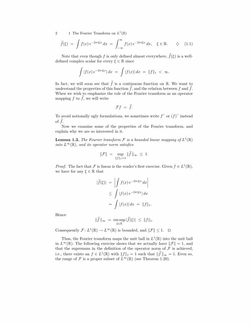
Lemma 1.2. The Fourier transform F is a bounded linear mapping of L1(R)into L∞(R), and its operator norm satisfies
‖F‖ = sup‖f‖1=1
‖f ‖∞ ≤ 1.
Proof. The fact that F is linear is the reader’s first exercise. Given f ∈ L1(R),we have for any ξ ∈ R that
|f(ξ)| =
∣∣∣∣∫
f(x) e−2πiξx dx
∣∣∣∣
≤∫
|f(x) e−2πiξx| dx
=
∫|f(x)| dx = ‖f‖1.
Hence‖f ‖∞ = ess sup
ξ∈R
|f(ξ)| ≤ ‖f‖1.
Consequently F : L1(R) → L∞(R) is bounded, and ‖F‖ ≤ 1. ⊓⊔
Thus, the Fourier transform maps the unit ball in L1(R) into the unit ballin L∞(R). The following exercise shows that we actually have ‖F‖ = 1, andthat the supremum in the definition of the operator norm of F is achieved,
i.e., there exists an f ∈ L1(R) with ‖f‖1 = 1 such that ‖f ‖∞ = 1. Even so,the range of F is a proper subset of L∞(R) (see Theorem 1.20).
1.1 Definition and Basic Properties 3
Exercise 1.3. Show that if f ∈ L1(R) then we have the useful fact that
f(0) =
∫f(x) dx.
Assume for now that f is continuous (we will prove this in Exercise 1.8), and
use this equality to show that if f ≥ 0 a.e., then ‖f ‖∞ = ‖f‖1. Conclude that‖F‖ = 1. ♦
Remark 1.4. There are many other standard normalizations for the Fouriertransform. For example, each of
∫f(x) e2πiξx dx,
∫f(x) e−iξx dx,
1√2π
∫f(x) e−iξx dx,
is a common choice. Each normalization makes certain formulas notationallynicer and other formulas more notationally complicated. ♦
We introduce a convenient notation for the dilation of a function.
Notation 1.5 (Dilation). Given a function f : R → C and given r > 0, wedefine the L1-normalized dilation of f by r to be the function fr : R → C
given byfr(x) = rf(rx). ♦
The dilation fr is L1-normalized in the sense that it preserves the L1
norm, i.e., ‖fr‖1 = ‖f‖1. When r < 1, the function fr is a “stretched out”version of f, while when r > 1, the function fr is a “shrunken” version of f,both with a vertical scaling that ensure that the L1-norm is preserved. Whenr > 1, it may be more descriptive to refer to fr as a compression of f, but itis customary to use the term dilation to refer to fr for all values of r.
Although there is the possibility of ambiguity between the notation forthe dilation fr of a function f and an element fn of a sequence of functionsfnn∈N, the meaning will usually be clear from context.
It is about time that we see a specific example of a Fourier transform.
Definition 1.6 (Dirichlet and Sinc Functions). The Dirichlet function is
d(ξ) =sin ξ
πξ
(implicitly defined at the origin so as to be continuous on R). The sinc functionis
sinc(ξ) =sin πξ
πξ= πd(πξ) = dπ(ξ). ♦
4 1 The Fourier Transform on L1(R)
-6 -4 -2 2 4 6-0.2
0.2
0.4
0.6
0.8
1.0
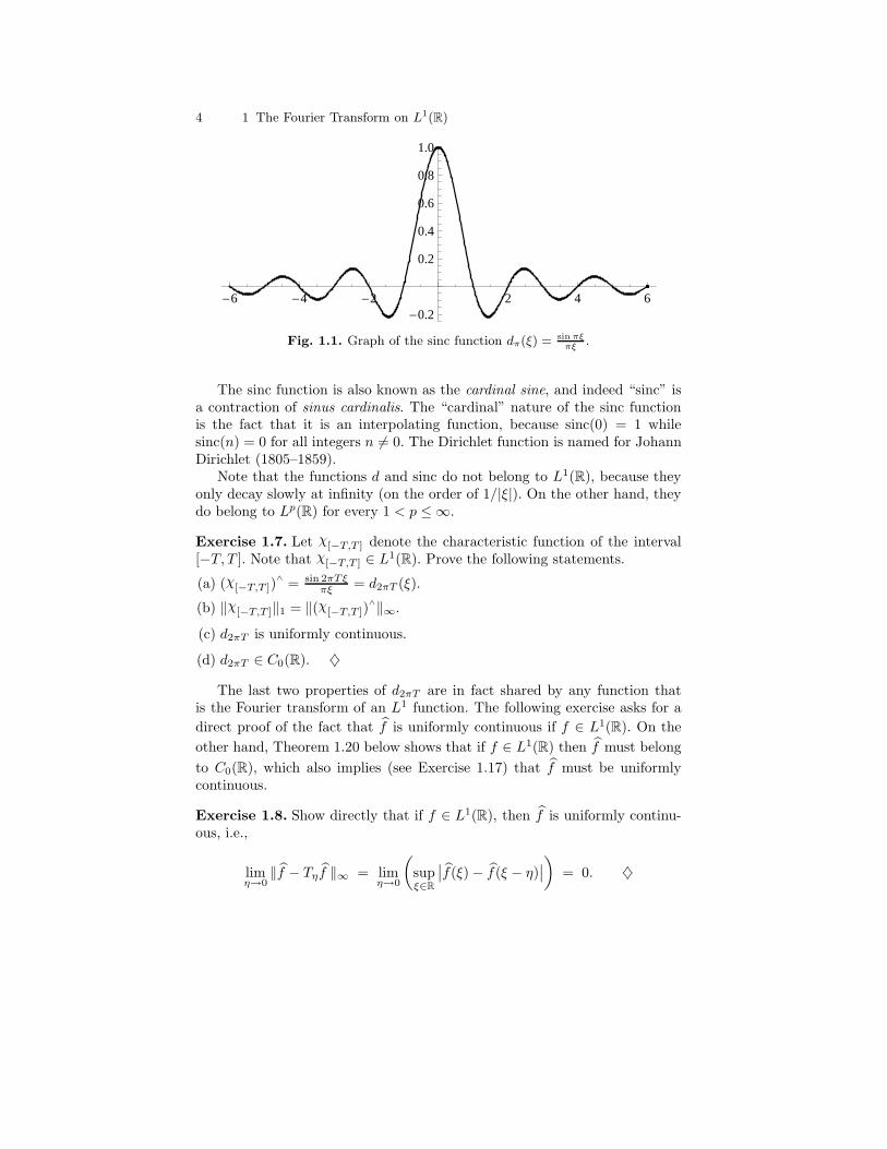
Fig. 1.1. Graph of the sinc function dπ(ξ) = sin πξ
πξ.
The sinc function is also known as the cardinal sine, and indeed “sinc” isa contraction of sinus cardinalis. The “cardinal” nature of the sinc functionis the fact that it is an interpolating function, because sinc(0) = 1 whilesinc(n) = 0 for all integers n 6= 0. The Dirichlet function is named for JohannDirichlet (1805–1859).
Note that the functions d and sinc do not belong to L1(R), because theyonly decay slowly at infinity (on the order of 1/|ξ|). On the other hand, theydo belong to Lp(R) for every 1 < p ≤ ∞.
Exercise 1.7. Let χ[−T,T ] denote the characteristic function of the interval[−T, T ]. Note that χ[−T,T ] ∈ L1(R). Prove the following statements.
(a) (χ[−T,T ])∧
= sin 2πTξπξ = d2πT (ξ).
(b) ‖χ[−T,T ]‖1 = ‖(χ[−T,T ])∧‖∞.
(c) d2πT is uniformly continuous.
(d) d2πT ∈ C0(R). ♦
The last two properties of d2πT are in fact shared by any function thatis the Fourier transform of an L1 function. The following exercise asks for a
direct proof of the fact that f is uniformly continuous if f ∈ L1(R). On the
other hand, Theorem 1.20 below shows that if f ∈ L1(R) then f must belong
to C0(R), which also implies (see Exercise 1.17) that f must be uniformlycontinuous.
Exercise 1.8. Show directly that if f ∈ L1(R), then f is uniformly continu-ous, i.e.,
limη→0
‖f − Tηf ‖∞ = limη→0
(supξ∈R
∣∣f(ξ) − f(ξ − η)∣∣)
= 0. ♦
1.1 Definition and Basic Properties 5
0
1
2
3
4
1
0
-1
0
1
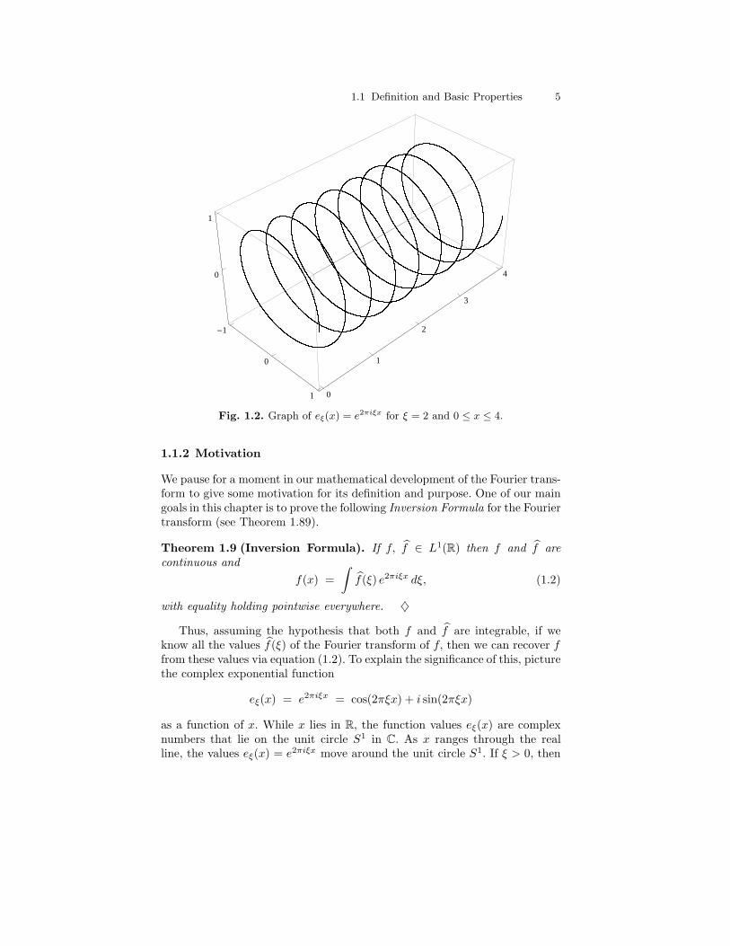
Fig. 1.2. Graph of eξ(x) = e2πiξx for ξ = 2 and 0 ≤ x ≤ 4.
1.1.2 Motivation
We pause for a moment in our mathematical development of the Fourier trans-form to give some motivation for its definition and purpose. One of our maingoals in this chapter is to prove the following Inversion Formula for the Fouriertransform (see Theorem 1.89).
Theorem 1.9 (Inversion Formula). If f, f ∈ L1(R) then f and f arecontinuous and
f(x) =
∫f(ξ) e2πiξx dξ, (1.2)
with equality holding pointwise everywhere. ♦
Thus, assuming the hypothesis that both f and f are integrable, if weknow all the values f(ξ) of the Fourier transform of f, then we can recover ffrom these values via equation (1.2). To explain the significance of this, picturethe complex exponential function
eξ(x) = e2πiξx = cos(2πξx) + i sin(2πξx)
as a function of x. While x lies in R, the function values eξ(x) are complexnumbers that lie on the unit circle S1 in C. As x ranges through the realline, the values eξ(x) = e2πiξx move around the unit circle S1. If ξ > 0, then

6 1 The Fourier Transform on L1(R)
as x increases through an interval of length 1/ξ, the values eξ(x) = e2πiξx
move once around S1 in the counter-clockwise direction. Thus eξ is periodicwith period 1/ξ. If ξ is negative, the same is true except that the valueseξ(x) = e2πiξx circle around S1 in the opposite direction. The graph of eξ is
Γξ =(x, e2πiξx) : x ∈ R
⊆ R × C.
Identifying R × C with R × R2 = R3, the graph Γξ is a helix in R3 coilingaround the x-axis, which runs down the center of the helix (see Figure 1.2).The function eξ is periodic with period 1/ξ, and we therefore say that it hasfrequency ξ, i.e., the frequency is the reciprocal of the period. The function eξ
is a “pure tone” or a “pure frequency” in some sense. Its real part is cos(2πξx),a cosine of period 1/ξ and frequency ξ. Its imaginary part is sin(2πξx), a sineof period 1/ξ and frequency ξ.
We turn to music for illustration. Restricting our attention for the mo-ment to real-valued functions, imagine that the function f(x) represents thedisplacement of the center of an ideal vibrating string, or the end of an idealtuning fork, or the center of your stereo speaker, from its rest position. Thevibrating string, tuning fork, or speaker creates a pressure wave in the air,which causes your eardrum to vibrate and your brain to perceive sound. Forthe function cos(2πξx), the sound that you would hear is a “pure tone” of fre-quency ξ. Real strings are of course much more complicated—a piano stringor a violin string each vibrates in a very complicated way, resulting in theirdifferent sounds. But an ideal string or tuning fork whose displacement is ex-actly given by the function cos(2πξx) would be a pure tone, with no overtonesor other complications (see the illustration in Figure 1.3). The function e2πiξx
is a complex version of this pure tone.
0.2 0.4 0.6 0.8 1.0
-1.0
-0.5
0.5
1.0
Fig. 1.3. Graph of ϕ(x) = cos(2π√
7x).
For a given fixed ξ, the function f(ξ) e2πiξx is a pure tone whose amplitude
is the scalar f(ξ). The larger f(ξ) is, the larger the vibrations of our string ortuning fork, and the louder the perceived sound.
1.1 Definition and Basic Properties 7
0.2 0.4 0.6 0.8 1.0
-3
-2
-1
1
2
3
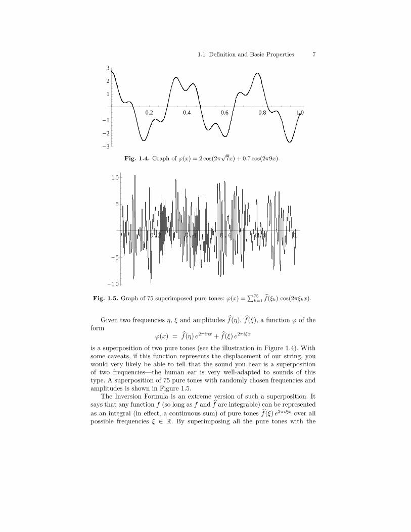
Fig. 1.4. Graph of ϕ(x) = 2 cos(2π√
7x) + 0.7 cos(2π9x).
0.2 0.4 0.6 0.8 1
-10
-5
5
10
Fig. 1.5. Graph of 75 superimposed pure tones: ϕ(x) =P75
k=1bf(ξk) cos(2πξkx).
Given two frequencies η, ξ and amplitudes f(η), f(ξ), a function ϕ of theform
ϕ(x) = f(η) e2πiηx + f(ξ) e2πiξx
is a superposition of two pure tones (see the illustration in Figure 1.4). Withsome caveats, if this function represents the displacement of our string, youwould very likely be able to tell that the sound you hear is a superpositionof two frequencies—the human ear is very well-adapted to sounds of thistype. A superposition of 75 pure tones with randomly chosen frequencies andamplitudes is shown in Figure 1.5.
The Inversion Formula is an extreme version of such a superposition. Itsays that any function f (so long as f and f are integrable) can be represented
as an integral (in effect, a continuous sum) of pure tones f(ξ) e2πiξx over allpossible frequencies ξ ∈ R. By superimposing all the pure tones with the

8 1 The Fourier Transform on L1(R)
correct amplitudes, we create any sound that we like. The pure tones are oursimple “building blocks,” and by combining them we can create any sound(or signal, or function). Of course, the “superposition” is an integral, not afinite sum, but still we are combining our very simple special functions eξ tocreate very complicated functions f via the Inversion Formula.
Once we have a representation of f in terms of our pure tones, we canact on it. For example, assume that we measure time in seconds, in whichcase frequency is usually called hertz. If we don’t like the annoying buzz inour signal f that is due to our 60 hertz overhead fluorescent lights, we mightdecide to modify f by creating a new function h whose Fourier transform isidentical to f except that h(60) = 0 (and most likely with some correspondingsmooth modifications of the frequencies close to ξ = 60 as well). Once we
know what we want h to be, the function h that does this is given by theInversion Formula as h(x) =
∫h(ξ) e2πiξx dξ. In engineering jargon, we filter f
to obtain h. We will see later that h can be obtained from f through theoperation of convolution (see Section 1.3.4).
In light of the Inversion Formula, we make the following definition.
Definition 1.10 (Inverse Fourier Transform). The inverse Fourier trans-form of f ∈ L1(R) is
∨
f (ξ) =
∫f(x) e2πiξx dx.
When we wish to denote the inverse Fourier transform as an operator acting
on f, we write F−1(f) =∨
f . ♦
Using this notation, the Inversion Formula says that if f, f ∈ L1(R) then
f =(f
)∨, and likewise f =
( ∨
f)∧
will hold under the same hypotheses.
Remark 1.11. If f ∈ L1(R) then∧
f (ξ) =∨
f (−ξ). Therefore, every result thatwe prove about the Fourier transform has an analogue for the inverse Fouriertransform, simply by making a change of variables. We usually only stateresults for the Fourier transform, but it is a good idea for the reader to workout the corresponding formulas for the inverse Fourier transform (usually, asign simply has to be moved from one place to another). Note, for example,
that if f, f ∈ L1(R), then the Inversion Formula tells us that
f∧∧
(ξ) =(f
)∨(−ξ) = f(−ξ). ♦
The musical discussion above may explain some terminology. In our ex-ample, the function f(x) represented a displacement (of a string or speaker)that changed with time. Time is represented by the variable x, and thus weoften speak of x as the time variable, and we say that values f(x) describe
the function f in the time domain. On the other hand, f(ξ) represents the“amount” of frequency ξ present in f, and therefore we often refer to ξ asthe frequency variable, and say that values f(ξ) describe the function f in the
1.1 Definition and Basic Properties 9
frequency domain. We use this terminology even if x represents somethingother than time and ξ something other than frequency. For example, we oftenuse this same terminology when we move to higher dimensions, i.e., even if fis defined on R2 instead of R, we might refer to R2 as the “time domain.” Or,if x is representing a spatial quantity, we may refer to R2 as the “spatial do-main.” There is no single perfect terminology since there are so many differentcontexts in which the Fourier transform can arise.
Additional Problems
1.1. Show that the Fourier transform of the one-sided exponential f(x) =e−x χ[0,∞)(x) is
f(ξ) =1
2πiξ + 1, ξ ∈ R,
and the Fourier transform of the two-sided exponential g(x) = e−|x| is
g(ξ) =2
4π2ξ2 + 1, ξ ∈ R.
1.2. Prove that if f ∈ L1(R) is even, then f is even, and if f ∈ L1(R) is
odd, then f is odd. The converse is also true, but is not as easy to prove, seeProblem 1.46.
1.3. Prove that if f ∈ L1(R) is real-valued, then f(ξ) = f(−ξ). Conclude that
if f is both real and even, then f is both real and even as well.
1.4. Show that if f ∈ L1(R) is nonnegative almost everywhere (and is not the
zero function), then |f(ξ)| < f(0) for all ξ 6= 0.
1.5. (a) The Gamma function for complex numbers z satisfying Re(z) > 0 is
Γ(z) =
∫ ∞
0
tz−1 e−t dt.
Show that this is well-defined, i.e., tz−1 e−t ∈ L1(0,∞) whenever Re(z) > 0.Remark: The Gamma function is analytic on Re(z) > 0, and has an ana-
lytic continuation to C \ 0,−1,−2, . . .. Also, Γ(n + 1) = n! for n ∈ N.
(b) Show that f(x) = e−ex
ex ∈ L1(R), and f(ξ) = Γ(1 − 2πiξ).Remark: It can be shown that Γ(z) 6= 0 for every z where it is defined, so
for this f we have f(ξ) 6= 0 for every ξ ∈ R.
1.6. The Riemann zeta function for complex numbers s with Re(s) > 1 is
ζ(s) =
∞∑
n=1
1
ns.

10 1 The Fourier Transform on L1(R)
The Riemann zeta function is analytic on Re(s) > 1, and has an analyticcontinuation to C \ 1. The Riemann hypothesis, whose validity is one of thegreat open problems in mathematics, states that if ζ(s) = 0 and Re(s) > 0then Re(s) = 1/2.
(a) Show that
(1 − 21−s) ζ(s) =
∞∑
n=1
(−1)n+1
ns, Re(s) > 1. (1.3)
(b) The right-hand side of equation (1.3) is an example of a Dirichletseries, and it converges and defines an analytic function on Re(s) > 0 (seeTheorem F.6). The left-hand side of equation (1.3) is analytic on Re(s) > 0except for s = 1, and can be defined so that it is analytic at s = 1 as well.Since both sides are analytic on Re(s) > 0 and are equal on Re(s) > 1, itfollows from the properties of analytic functions that equation (1.3) holds forall s with Re(s) > 0. For s = 1 we need to define the left-hand side to take
the value∑ (−1)n+1
n = ln 2. Assuming these facts, show that
Γ(s) (1 − 21−s) ζ(s) =
∞∑
n=1
(−1)n+1
∫ ∞
0
xs−1 e−nx dx, Re(s) > 0. (1.4)
It is helpful to note that, by a change of variables, Γ(s) = ns∫ ∞
0 xs−1 e−nx dxfor Re(s) > 0.
(c) Justify interchanging the summation and integral in equation (1.4) toobtain
Γ(s) (1 − 21−s) ζ(s) =
∫ ∞
0
xs−1 1
ex + 1dx, Re(s) > 0.
(d) Given t > 0, define
ft(x) =etx
eex + 1.
Show that ft ∈ L1(R). Given ξ ∈ R, let s = t − 2πiξ and show that
ft(ξ) = Γ(s) (1 − 21−s) ζ(s).
1.2 Translation, Modulation, Dilation, and Involution
A common theme of many of the issues that we will consider in this chapterconcerns the dualities that occur between properties of f and those of f . Inthis section we examine the dualities that occur among several basic operatorsunder the Fourier transform.

1.2 Translation, Modulation, Dilation, and Involution 11
1.2.1 Four Fundamental Operators
Here are four operators that will pervade our study of the Fourier transform.
Definition 1.12. We define the following operators on functions f : R → C.
Translation: (Taf)(x) = f(x − a), a ∈ R.
Modulation: (Mθf)(x) = e2πiθxf(x), θ ∈ R.
Dilation: fλ(x) = λf(λx), λ > 0.
Involution: f(x) = f(−x). ♦
The scaling factor in the definition of dilation has been chosen so that di-lation preserves the L1-norm of a function. Translation, modulation, dilation,and involution are all isometries mapping L1(R) onto itself.
Exercise 1.13. Prove the following algebraic properties of the Fourier trans-form of f ∈ L1(R).
(a) (Taf)∧
(ξ) = (M−af )(ξ) = e−2πiaξ f(ξ), for a ∈ R.
(b) (Mηf)∧
(ξ) = (Tηf )(ξ) = f(ξ − η), for η ∈ R.
(c) (fλ)∧
(ξ) = λ (f )1/λ(ξ) = f(ξ/λ), for λ > 0.
(d) (f )∧
(ξ) = (f )∼(ξ) = f(−ξ).
(e) (f )∧
(ξ) = f(ξ).
Also derive analogous formulas relating the inverse Fourier transform to trans-lation, modulation, dilation, and involution. ♦
In this sense, Ta is dual to M−a under the Fourier transform, and likewiseMη is dual to Tη. Additionally, except for the normalizing scaling factor (whichwill be very important to us in Section 1.5!), dilation by λ is dual to dilationby 1/λ under the Fourier transform.
In order to derive some of the properties of the family of translation op-erators, it is helpful to know that Cc(R) is dense in Lp(R) when p is finite.We will prove this using standard real analysis techniques. By making use ofconvolutions, we will greatly refine this result in Section 1.5. For example, wewill see that the seemingly “tiny” space C∞
c (R) is dense in Lp(R) for each1 ≤ p < ∞, and is dense in C0(R) with respect to the L∞-norm.
The tool that we need for this proof is Urysohn’s Lemma, a general topolog-ical result which states that if A and B are disjoint closed subsets of a normaltopological space X then there exists a continuous function f : X → [0, 1] thatis identically 0 on A and identically 1 on B. We will prove Urysohn’s Lemmafor subsets of Rd (although the same simple proof can be used in any metricspace). The key is the following lemma.
12 1 The Fourier Transform on L1(R)
Lemma 1.14. If E ⊆ Rd is nonempty, then
f(x) = dist(x, E) = inf|x − z| : z ∈ E
is uniformly continuous on Rd.
Proof. Fix ε > 0. Choose any x, y ∈ Rd with |x−y| < ε/2. By definition, thereexist a, b ∈ E such that |x−a| < dist(x, E)+ε/2 and |y−b| < dist(y, E)+ε/2.Hence
f(y) = dist(y, A) ≤ |y − a|
≤ |y − x| + |x − a|
<ε
2+ dist(x, E) +
ε
2
= f(x) + ε.
Similarly f(x) < f(y) + ε, so |f(x) − f(y)| < ε whenever |x − y| < ε/2. ⊓⊔
Theorem 1.15 (Urysohn’s Lemma). If E, F are disjoint closed subsets ofRd, then there exists a continuous function θ : Rd → R such that
(a) 0 ≤ θ ≤ 1,
(b) θ = 0 on E, and
(c) θ = 1 on F.
Proof. Because E is closed, if x /∈ E then dist(x, E) > 0. Also, by Lemma 1.14,dist(x, E) and dist(x, F ) are each continuous functions of x. Therefore thefunction
θ(x) =dist(x, E)
dist(x, E) + dist(x, F )
has the required properties. ⊓⊔
Theorem 1.16. Cc(Rd) is dense in Lp(Rd) for each 1 ≤ p < ∞.
Proof. First consider the function f = χE where E ⊆ Rd is bounded. If we fixε > 0, then there exists a bounded open set U ⊇ E such that |U\E| < εand a compact set K ⊆ E such that |E\K| < ε. By Urysohn’s Lemma(Theorem 1.15), we can find a continuous function θ : Rd → R such that0 ≤ θ ≤ 1, θ = 1 on K, and θ = 0 on Rd\U. Then θ ∈ Cc(R
d), and we have
‖χE − θ‖pp =
∫|χE − θ|p =
∫
U\K
|χE − θ|p ≤ |U\K| < 2ε.
Hence χE can be approximated arbitrarily closely in Lp-norm by elementsof Cc(R
d). By forming finite linear combinations, it follows that every simplefunction in Lp(Rd) that has compact support can be approximated as well aswe like by functions in Cc(R
d). Since the set of compactly supported simplefunctions is dense in Lp(Rd), we conclude that Cc(R
d) is dense as well. ⊓⊔
1.2 Translation, Modulation, Dilation, and Involution 13
Now we establish some properties of the translation operator Ta. The“easy” way to prove part (c) of the next exercise is to first prove that it holdsfor functions in Cc(R), and then use the fact that Cc(R) is dense to extend toLp(R).
Exercise 1.17. (a) Prove that if f ∈ C0(R) then f is uniformly continuous,and show that this is equivalent to the statement
lima→0
‖Taf − f‖∞ = 0. (1.5)
(b) Show that (1.5) can fail if we only assume that f ∈ Cb(R).
(c) Show that if 1 ≤ p < ∞ and f ∈ Lp(R), then
lima→0
‖Taf − f‖p = 0. ♦
The function ωp(a) = ‖Taf − f‖p is often called the Lp-modulus of conti-nuity of f.
Remark 1.18. If we consider the linear mapping τ : R → B(Lp(R)) defined byτ(a) = Ta, then Exercise 1.17 implies that for each 1 ≤ p < ∞ we have
∀ f ∈ Lp(R), limt→s
‖τ(t)f − τ(s)f‖p = 0.
In another terminology, this says that τ(t) → τ(s) in the strong operatortopology as t → s. For 1 ≤ p < ∞, we therefore say that Taa∈R is a stronglycontinuous one-parameter family of operators on Lp(R). The same is true ofTaa∈R on C0(R) when p = ∞. ♦
Exercise 1.19. Prove that the family Mηη∈R of modulation operators is astrongly continuous family of operators on Lp(R) for 1 ≤ p < ∞. For p = ∞,show that Mηη∈R is a strongly continuous family on C0(R), but not onL∞(R). ♦
1.2.2 The Riemann–Lebesgue Lemma
We now use the strong continuity of the family of translation operators toprove that if f ∈ L1(R), then not only is f continuous, but we also have decay
of f at infinity.
Theorem 1.20 (Riemann–Lebesgue Lemma). If f ∈ L1(R), then f ∈C0(R).
Proof. Choose any f ∈ L1(R). We already know that f is continuous, so wejust have to show that it decays at infinity. Since e−πi = −1, we have for ξ 6= 0that
14 1 The Fourier Transform on L1(R)
f(ξ) =
∫f(x) e−2πiξx dx (1.6)
= −∫
f(x) e−2πiξx e−2πiξ( 12ξ
) dx
= −∫
f(x) e−2πiξ(x+ 12ξ
) dx
= −∫
f(x − 1
2ξ
)e−2πiξx dx. (1.7)
Averaging equalities (1.6) and (1.7), we obtain
f(ξ) =1
2
∫ (f(x) − f
(x − 1
2ξ
))e−2πiξx dx.
The fact that translation is strongly continuous on L1(R) therefore impliesthat
|f(ξ)| ≤ 1
2
∫ ∣∣∣f(x) − f(x − 1
2ξ
)∣∣∣ dx =1
2‖f − T 1
2ξf‖1 → 0
as |ξ| → ∞. ⊓⊔While certainly elegant, and yielding the nice L1-modulus of continuity
estimate
|f(ξ)| ≤ 1
2w1
( 1
2ξ
),
the preceding proof does have a less-than-satisfying “magical” feel to it. Adifferent proof of the Riemann–Lebesgue Lemma is given in Problem 1.8, anda third proof appears in Section 1.4.
1.2.3 Position and Momentum
Two addition operators that play central roles in harmonic analysis are themathematical versions of the position and momentum operators from quan-tum mechanics. These are defined as follows.
Definition 1.21 (Position and Momentum). The position and momen-tum operators P and M are
Pf(x) = xf(x), and Mf =1
2πif ′. ♦ (1.8)
The position operator is defined on all functions f : R → C. The momen-tum operator is defined on all differentiable functions f, although often weonly require that Mf be defined almost everywhere and hence only need toassume that f is differentiable at almost every point.
Unlike the translation, modulation, dilation, and involution operators, theposition and momentum operators do not map Lp(T) boundedly into itself,even if we restrict to domains where they are well-defined (see Problem 1.9).Even so, Problems 1.11 and 1.12 show that position and momentum are fun-damentally tied to modulation and translation.
1.2 Translation, Modulation, Dilation, and Involution 15
1.2.4 The HRT Conjecture
We close or discussion of translation and modulation by briefly discussing oneof our favorite open mathematical problems.
Conjecture 1.22 (The HRT Conjecture). If g ∈ L2(R) is not the zerofunction and Λ = (pk, qk)N
k=1 is any set of finitely many distinct points inR2, then
G(g, Λ) =Mqk
TpkgN
k=1
is a linearly independent set of functions in L2(R). ♦
Conjecture 1.22 was first made in [HRT96]. While many partial resultsrelated to this conjecture are known, as of the time of writing it is not knownwhether Conjecture 1.22 holds in the generality stated. For more details andbackground on this conjecture, we refer to the survey paper [Heil06] or Section11.9 in the author’s text [Heil11a].
Additional Problems
1.7. Let f : R → C be Lebesgue measurable. Prove that Tafm→ f (convergence
in measure) as a → 0 on any compact set, i.e.,
∀ compact K ⊆ R, ∀ ε > 0, lima→0
∣∣x ∈ K : |f(x) − Taf(x)| > ε∣∣ = 0.
1.8. This problem provides an alternative proof to Theorem 1.20.
(a) Show that f ∈ C0(R) for every f ∈ S = spanχ[a,b] : a < b ∈ R.(b) Show that S is dense in L1(R) and use this to prove that f ∈ C0(R)
for every f ∈ L1(R).
1.9. Let P, M be the position and momentum operators defined in equation(1.8), and fix 1 ≤ p < ∞. These operators are not defined on all of Lp(R).Instead, define domains
DP = f ∈ Lp(R) : xf(x) ∈ Lp(R),DM = f ∈ Lp(R) : f is differentiable and f ′ ∈ Lp(R),
which are dense subspaces of Lp(R). Restricted to these domains, P maps DP
into Lp(R) and M maps DM into Lp(R). Show that P and M are unboundedeven when restricted to these domains, i.e.,
supf∈DP ,‖f‖p=1
‖Pf‖p = ∞ = supf∈DM ,‖f‖p=1
‖Mf‖p.

16 1 The Fourier Transform on L1(R)
1.10. Let X be a Banach space, and fix A ∈ B(X). For n > 0 let An denotethe usual nth power of A (An = A · · ·A, n times), and define A0 = I (theidentity map on X).
(a) Given x ∈ X, show that the series eA(x) =∑∞
k=0Akxk! converges abso-
lutely in X, and show that eA is a linear operator on X.
(b) Prove that the series∑∞
k=0Ak
k! converges absolutely in B(X), andequals the operator eA defined in part (a). Conclude that eA ∈ B(X) and
‖eA‖ ≤ e‖A‖.
(c) Prove that if A, B ∈ B(X) and AB = BA, then eAeB = eA+B = eBeA.
(d) Let H be a Hilbert space. Show that if A ∈ B(H) is self-adjoint, theneiA is unitary.
1.11. Show that for an appropriate dense subset of functions f ∈ L1(R) wehave
Mξf = e2πiξP f =
∞∑
k=0
(2πiξP )kf
k!,
and similarly there is a set of f ∈ L1(R) such that
Taf = e−2πiaMf =
∞∑
k=0
(−2πiaM)kf
k!,
where these series converge absolutely both in the pointwise sense and in L1-norm. In contrast to Problem 1.10, note that the operators P and M areunbounded on L1(R).
1.12. Show that for an appropriate dense subset functions f ∈ L1(R) we have
2πiMf = lima→0
f − Taf
aand − 2πiPf = lim
ξ→0
f − Mξf
ξ, (1.9)
where these limits converge both in the pointwise sense and in L1-norm.
Remark: Equation (1.9) says that 2πiM is the infinitesimal generator ofthe strongly continuous family of operators Taa∈R, and −2πiP is the in-finitesimal generator of the family Mξξ∈R.
1.3 Convolution
Since L1(R) is a Banach space, we know that it has many useful properties. Inparticular the operations of addition and scalar multiplication are continuous.However, there are many other operations on L1(R) that we could consider.One natural operation is multiplication of functions, but unfortunately L1(R)is not closed under pointwise multiplication.

1.3 Convolution 17
Exercise 1.23. Show that f, g ∈ L1(R) does not imply fg ∈ L1(R). ♦
In this section we will define a different “multiplication-like” operationunder which L1(R) is closed. This operation, convolution of functions, willbe one of the most important tools in our further development of harmonicanalysis. Therefore, in this section we set aside the Fourier transform for themoment, and concentrate on developing the machinery of convolution.
1.3.1 Some Notational Conventions
Before proceeding, there are some technical issues related to the definition ofelements of Lp(R) that we need to clarify.
The basic source of difficulty is that an element f of Lp(R) is not a func-tion but rather denotes an equivalence class of functions that are equal almosteverywhere. Therefore we cannot speak of the “value of f ∈ Lp(R) at a pointx ∈ R,” and consequently concepts such as continuity or support do not ap-ply in a literal sense to elements of Lp(R). For example, the zero function0 and the function χ
Q both belong to the zero element of Lp(R), which isthe equivalence class of functions that are zero a.e., yet 0 is continuous andcompactly supported while χ
Q is discontinuous and its support is R. Even so,it is often essential to consider smoothness or support properties of functions,and we therefore adopt the following conventions when discussing the smooth-ness or support of elements of Lp(R). More generally, these same issues andconventions apply to elements of
L1loc(R) =
f : R → C : f · χK ∈ L1(R) for every compact K ⊆ R
,
which is the space of locally integrable functions on R. Note that Lp(R) ⊆L1
loc(R) for every 1 ≤ p ≤ ∞.
Notation 1.24 (Continuity for Elements of L1loc(R)). We will say that
f ∈ L1loc(R) is continuous if there is a representative of f that is continuous,
i.e., there exists some continuous function f0 such that f is the equivalenceclass of all functions that equal f0 almost everywhere.
Conversely, if g is a continuous function such that∫
K|g(x)| dx < ∞ for
every compact K ⊆ R, then we write g ∈ L1loc(R) with understanding that this
means that the equivalence class of functions that equal g a.e. is an elementof L1
loc(R). In this sense we write statements such as Cc(R) ⊆ Lp(R) eventhough Cc(R) is a set of functions while Lp(R) is a set of equivalence classesof functions. ♦
Notation 1.25 (Support of Elements of L1loc(R)). We will say that f ∈
L1loc(R) has compact support if there is a representative of f that has compact
support. Thus f has compact support if there exists an N > 0 such thatf(x) = 0 for a.e. |x| > N.

18 1 The Fourier Transform on L1(R)
In many situations, this definition of compact support is all that we need,but in some circumstances it is important to discuss the support of f ∈ L1
loc(R)explicitly. We define the support of f ∈ L1
loc(R) to be
supp(f) =⋂
F ⊆ R : F is closed and f(x) = 0 for a.e. x /∈ F.
In particular, if F is a closed subset of R, then
supp(f) ⊆ F ⇐⇒ f(x) = 0 for a.e. x /∈ F.
However, if T is a generic subset of R, then the statements supp(f) ⊆ T andf(x) = 0 for a.e. x /∈ T need not be equivalent.
In the language of Chapter 4, we are taking the support of f ∈ L1loc(R)
to be the support of the distribution in D′(R) that is determined by f, seeSection 4.6. ♦
The reader should verify that if f ∈ L1loc(R) is continuous (in the sense
given in Notation 1.24), then the support of f in the sense of Notation 1.25coincides with the usual definition of the support of f as the closure in R ofthe set x ∈ R : f(x) 6= 0.
1.3.2 Definition and Basic Properties of Convolution
Now we can define convolution of functions.
Definition 1.26 (Convolution). Let f : R → C and g : R → C be Lebesguemeasurable functions. Then the convolution of f with g is the function f ∗ ggiven by
(f ∗ g)(x) =
∫f(y) g(x − y) dy, (1.10)
whenever this integral is well-defined. ♦
For example, suppose that 1 ≤ p ≤ ∞ and let p′ be the dual index to p.If f ∈ Lp(R) and g ∈ Lp′
(R), then (as functions of y), f(y) and g(x − y)belong to dual spaces, and hence by Holder’s Inequality the integral defining(f ∗ g)(x) in equation (1.10) exists for every x, and furthermore is boundedas a function of x.
Exercise 1.27. Show that if 1 ≤ p ≤ ∞, f ∈ Lp(R), and g ∈ Lp′
(R), thenf ∗ g ∈ L∞(R), and we have
‖f ∗ g‖∞ ≤ ‖f‖p ‖g‖p′. (1.11)
We will improve on this exercise (in several ways) below. In particular,Exercise 1.27 does not give the only hypotheses on f and g which implythat f ∗ g exists—we will shortly see Young’s Inequality, which is a powerfulresult that tells us that f ∗ g will belong to a particular Lebesgue space Lr(R)

1.3 Convolution 19
whenever f ∈ Lp(R), g ∈ Lq(R), and we have the proper relationship amongp, q, and r (specifically, 1
p + 1q = 1 + 1
r ). Before turning to that general case,
we prove the fundamental fact that L1(R) is closed under convolution, andthat the Fourier transform interchanges convolution with multiplication.
Theorem 1.28. If f, g ∈ L1(R) are given, then the following statements hold.
(a) f(y) g(x − y) is Lebesgue measurable on R2.
(b) For almost every x ∈ R, f(y) g(x − y) is a measurable and integrablefunction of y, and hence (f ∗ g)(x) is defined for a.e. x ∈ R.
(c) f ∗ g ∈ L1(R), and‖f ∗ g‖1 ≤ ‖f‖1 ‖g‖1.
(d) The Fourier transform of f ∗ g is the product of the Fourier transformsof f and g:
(f ∗ g)∧
(ξ) = f(ξ) g(ξ), ξ ∈ R.
Proof. (a) If we set h(x, y) = f(x), then
h−1(a,∞) = (x, y) : h(x, y) > a = (x, y) : f(x) > a = f−1(a,∞) × R,
which is a measurable subset of R2 since f−1(a,∞) and R are measurablesubsets of R. Likewise k(x, y) = g(y) is measurable. Since the product ofmeasurable functions is measurable, we conclude that F (x, y) = f(x)g(y)is measurable. Further, T (x, y) = (y, x − y) is a linear transformation, soH(x, y) = (F T )(x, y) = F (y, x − y) = f(y) g(x − y) is measurable.
(b) Using the same notation as in part (a), we have∫∫
|H(x, y)| dx dy =
∫ (∫|g(x − y)| dx
)|f(y)| dy
=
∫‖g‖1 |f(y)| dy = ‖g‖1 ‖f‖1.
Therefore H(x, y) = f(y) g(x−y) ∈ L1(R2), so Fubini’s Theorem implies thatthe function (f ∗ g)(x) =
∫f(y) g(x − y) dy exists for almost every x and is
an integrable function of x.
(c) Using part (b),
‖f ∗ g‖1 =
∫|(f ∗ g)(x)| dx ≤
∫∫|f(y) g(x − y)| dy dx = ‖f‖1 ‖g‖1.
(d) Fubini’s Theorem (exercise: justify its use) allows us to interchangeintegrals in the following calculation:
(f ∗ g)∧
(ξ) =
∫(f ∗ g)(x) e−2πiξx dx
=
∫∫f(y) g(x − y) e−2πiξx dy dx
20 1 The Fourier Transform on L1(R)
=
∫f(y) e−2πiξy
(∫g(x − y) e−2πiξ(x−y) dx
)dy
=
∫f(y) e−2πiξy
(∫g(x) e−2πiξx dx
)dy
=
∫f(y) e−2πiξy g(ξ) dy
= f(ξ) g(ξ). ⊓⊔
In the proof of Theorem 1.28, we carefully addressed the measurability off ∗ g. We will usually take issues of measurability for granted from now on,but it is a good idea for the reader to consider wherever appropriate why themeasurability of the functions we encounter is ensured.
Exercise 1.29. Establish the following basic properties of convolution. Givenf, g, h ∈ L1(R), prove the following.
(a) Commutativity: f ∗ g = g ∗ f.
(b) Associativity: (f ∗ g) ∗ h = f ∗ (g ∗ h).
(c) Distributive laws: f ∗ (g + h) = f ∗ g + f ∗ h.
(d) Commutativity with translations: f ∗ (Tag) = (Taf) ∗ g = Ta(f ∗ g) fora ∈ R.
(e) Behavior under involution: (f ∗ g)∼ = f ∗ g. ♦
1.3.3 Young’s Inequality
As we have seen, L1(R) is closed under convolution, which we write in shortas
L1(R) ∗ L1(R) ⊆ L1(R).
It is not true that Lp(R) is closed under convolution for p > 1. Instead wehave the following fundamental result, known as Young’s Inequality (although,since Young proved many inequalities, it may be advisable to refer to this asYoung’s Convolution Inequality).
Exercise 1.30 (Young’s Inequality). Prove the following statements.
(a) If 1 ≤ p ≤ ∞ then Lp(R) ∗ L1(R) ⊆ Lp(R), and we have
∀ f ∈ Lp(R), ∀ g ∈ L1(R), ‖f ∗ g‖p ≤ ‖f‖p ‖g‖1. (1.12)
(b) If 1 ≤ p, q, r ≤ ∞ and 1r = 1
p + 1q − 1 then Lp(R) ∗ Lq(R) ⊆ Lr(R), and
we have
∀ f ∈ Lp(R), ∀ g ∈ Lq(R), ‖f ∗ g‖r ≤ ‖f‖p ‖g‖q. ♦ (1.13)
1.3 Convolution 21
Of course, statement (a) in Young’s Inequality is a special case of state-ment (b), but it is so useful that it is worth stating separately. It is alsoinstructive on first try to attempt to prove statement (a) rather than themore general statement (b) in order to see the appropriate technique needed.There are many ways to prove Young’s Inequality, e.g., via Holder’s Inequalityor Minkowski’s Integral Inequality (which is stated in Problem 1.25).
Remark 1.31. If q = p′ (in which case r = ∞), then Young’s Inequality tellsus that the convolution of f ∈ Lp(R) with g ∈ Lp′
(R) belongs to L∞(R). Infact, it follows from our later Exercise 1.39 that f ∗g is continuous in this case,and therefore (f ∗ g)(x) is defined for every x. However, for general values ofp, q, r satisfying the hypotheses of Young’s Inequality, we are only able toconclude that f ∗ g ∈ Lr(R), and hence we usually only have that f ∗ g isdefined pointwise almost everywhere. ♦
The inequalities given in Exercise 1.30 are in the form that we will mostoften need in practice, but it is very interesting to note that the implicitconstant 1 on the right-hand side of equation (1.13) is not the optimal constantin general. Instead, if we define the Babenko–Beckner constant Ap by
Ap =
(p1/p
p′1/p′
)1/2
, (1.14)
where we take A1 = A∞ = 1, then the optimal version of equation (1.13) is
∀ f ∈ Lp(R), ∀ g ∈ Lq(R), ‖f ∗ g‖r ≤ (ApAqAr′) ‖f‖p ‖g‖p, (1.15)
and the constant ApAqAr′ is typically not 1. The proof that ApAqAr′ is thebest constant in equation (1.15) is due to Beckner [Bec75] and Brascampand Lieb [BrL76]. The Babenko–Beckner constant will make an appearanceagain when we consider the Hausdorff–Young Theorem in Chapter 3 (seeTheorem 3.23).
1.3.4 Convolution as Filtering; Lack of an Identity
Theorem 1.28 gives us another way to view filtering (which was discussedin Section 1.1.2). Given f ∈ L1(R), we filter f by modifying its frequencycontent. That is, we create a new function h from f whose Fourier transformis
h(ξ) = f(ξ) g(ξ).
The Fourier transform of the function g tells us how to modify the frequencycontent of f. Assuming that the Inversion Formula applies, we can recover hby the formula
h(x) =
∫f(ξ) g(ξ) e2πiξx dξ,
22 1 The Fourier Transform on L1(R)
which is a superposition of the “pure tones” e2πiξx with the modified ampli-
tudes f(ξ) g(ξ). Assuming that g ∈ L1(R), Theorem 1.28 tells us that we canalso obtain h by convolution: we have h = f ∗ g. Filtering is convolution.
Obviously, there are many details that we are glossing over by assumingall of the formulas are applicable. Some of these we will address later, e.g.,is it true that a function h ∈ L1(R) is uniquely determined by its Fourier
transform h? (Yes, we will show that f 7→ f is an injective map of L1(R) intoC0(R), see Theorem 1.92.) Others we will leave for a course on digital signalprocessing. (For example, how do results for L1(R) relate to the processing ofreal-life digital signals whose domain is 1, . . . , n instead of R?) In any case,keeping our attention on the real line, let us ask one interesting question. Ifour goal is to filter f, then one of the possible filterings should be the identityoperation, i.e., do nothing to the frequency content of f. Is there a g ∈ L1(R)such that f 7→ f ∗ g is the identity operation on L1(R)?
Exercise 1.32. Suppose that there existed a function δ ∈ L1(R) such that
∀ f ∈ L1(R), f ∗ δ = f.
Show that δ would satisfy δ(ξ) = 1 for all ξ, which contradicts the Riemann–Lebesgue Lemma. ♦
Consequently, there is no identity element for convolution in L1(R). Thisis problematic, and we will see several alternative ways of addressing thisproblem. In Section 1.5, we will construct functions which “approximate” anidentity for convolution as closely as we like, according to a variety of meaningsof approximation. In Chapter 4, we will create a distribution (or “generalizedfunction”) δ that is not itself a function but instead acts on functions andis an identity with respect to convolution. In Chapter 5, we will see thatthis distribution δ can also be regarded as a bounded measure on the realline. Thus, while there is no function δ that is an identity for convolution, anidentity δ does exist in several generalized senses.
1.3.5 Convolution as Averaging; Introduction to ApproximateIdentities
Convolution can also be regarded as a kind of weighted averaging operator.For example, consider
χT =1
2Tχ[−T,T ], T > 0.
Given f ∈ L1(R), we have that
(f ∗ χT )(x) =
∫f(y)χT (x − y) dy =
1
2T
∫ x+T
x−T
f(y) dy = AvgT f(x),

1.3 Convolution 23
T
x - T x T + x
Avg f HxL
Fig. 1.6. The area of the dashed box equalsR x+T
x−Tf(y) dy, which is the area under
the graph of f between x − T and x + T.
where AvgT f(x) is the average of f on the interval [x − T, x + T ] (see Fig-ure 1.6).
For a general function g, the mapping f 7→ f ∗ g can be regarded as a kindof weighted averaging of f, with g weighting some parts of the real line morethan others. There is one technical point to observe in this viewpoint: whilethe function χT (x) = 1
2Tχ[−T,T ] used in the preceding illustration is even,
this will not be the case in general. Instead, in thinking of convolution as aweighted averaging, it is perhaps better to set g∗(x) = g(−x) and write
(f ∗ g)(x) =
∫f(y) g∗(y − x) dy = Avgg∗f(x),
the average of f around the point x corresponding to the weighting of thereal line by g∗(x) = g(−x). Alternatively, since convolution is commutative,we can equally view it as an averaging of g using the weighting correspondingto f∗(x) = f(−x).
Looking ahead to Section 1.5, let us consider what happens to the convo-lution f ∗ χT = AvgT f as T → 0. The function χT = 1
2Tχ[−T,T ] becomes a
taller and taller “spike” centered at the origin, with the height of the spikebeing chosen so that the integral of χT is always 1. Intuitively, averaging oversmaller and smaller intervals should give values (f ∗χT )(x) that are closer andcloser to the original value f(x). This intuition is made precise in Lebesgue’sDifferentiation Theorem (Theorem A.30), which implies that if f ∈ L1(R)then for almost every x (including all those in the Lebesgue set of f) we willhave
f(x) = limT→0
(f ∗ χT )(x) = limT→0
AvgT f(x).
Thus f ≈ f ∗ χT when T is small. In this sense, while there is no identityelement for convolution in L1(R), the function χT is approximately an iden-tity for convolution, and the approximation becomes better and better thesmaller T becomes.
Moreover, a similar phenomenon happens for the more general averagingoperators f 7→ f ∗g = Avgg∗f. We can take any particular function g ∈ L1(R)
24 1 The Fourier Transform on L1(R)
and dilate it so that it becomes more and more compressed towards the origin,yet always keeping the total integral the same, by setting
gλ(x) = λg(λx), λ > 0,
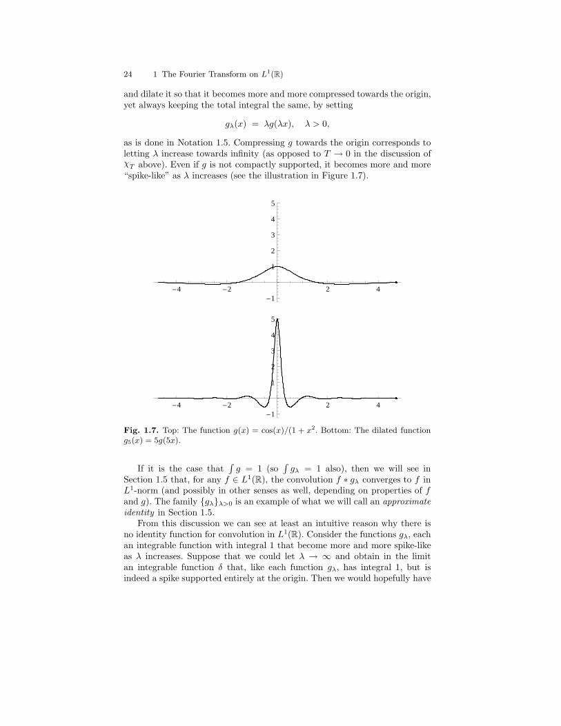
as is done in Notation 1.5. Compressing g towards the origin corresponds toletting λ increase towards infinity (as opposed to T → 0 in the discussion ofχT above). Even if g is not compactly supported, it becomes more and more“spike-like” as λ increases (see the illustration in Figure 1.7).
-4 -2 2 4-1
1
2
3
4
5
-4 -2 2 4-1
1
2
3
4
5
Fig. 1.7. Top: The function g(x) = cos(x)/(1 + x2. Bottom: The dilated functiong5(x) = 5g(5x).
If it is the case that∫
g = 1 (so∫
gλ = 1 also), then we will see inSection 1.5 that, for any f ∈ L1(R), the convolution f ∗ gλ converges to f inL1-norm (and possibly in other senses as well, depending on properties of fand g). The family gλλ>0 is an example of what we will call an approximateidentity in Section 1.5.
From this discussion we can see at least an intuitive reason why there isno identity function for convolution in L1(R). Consider the functions gλ, eachan integrable function with integral 1 that become more and more spike-likeas λ increases. Suppose that we could let λ → ∞ and obtain in the limitan integrable function δ that, like each function gλ, has integral 1, but isindeed a spike supported entirely at the origin. Then we would hopefully have

1.3 Convolution 25
that f ∗ δ = limλ→∞ f ∗ gλ = f, and so δ would be an identity function forconvolution. And indeed, it is not uncommon to see informal wording similarto the following.
“Let δ be the function on R that has the property that δ(x) = 0 forall x 6= 0 and
∫δ(x) dx = 1. Then
∫f(y) δ(x − y) dy = f(x).” (1.16)
However, there is no such function δ. Any function that is zero for all x 6= 0is zero almost everywhere, and hence is the zero element of L1(R). If δ(x) = 0for x 6= 0, then the Lebesgue integral of δ is
∫δ(x) dx = 0, not 1, even if we
define δ(0) = ∞. Thus f ∗ δ = 0, not f.We cannot construct a function δ that has the property that f∗δ = f for all
f ∈ L1(R). However, we can construct families gλλ>0 that have the propertythat f ∗ gλ converges to f in various senses, and these are the approximateidentities of Section 1.5. We can also construct objects that are not functionsbut which are identities for convolution—we will see the δ-distribution inChapter 4 and the δ-measure in Chapter 5. In effect, the integral appearingin equation (1.16) is not a Lebesgue integral but rather is simply a shorthandfor something else, namely, the action of the distribution or measure δ on thefunction f.
1.3.6 Convolution as an Inner Product
It is often useful to write a convolution in one of the following forms (the
involution g(x) = g(−x) was introduced in Definition 1.12):
(f ∗ g)(x) =
∫f(y) g(x − y) dy
=
∫f(y) g(y − x) dy
=
∫f(y)Txg(y) dy = 〈f, Txg 〉. (1.17)
Thus we can view the convolution of f with g at the point x as the innerproduct of f with the function g translated by x.
Notation 1.33. In equation (1.17), we have used the notation 〈·, ·〉, which inthe context of functions usually denotes the inner product on L2(R). However,neither f nor Txg need belong to L2(R), so we are certainly taking somepoetic license in speaking of 〈f, Txg 〉 as an inner product of f and Txg. Wedo this because in this volume we so often encounter integrals of the form∫
f(x) g(x) dx and direct generalizations of these integrals that it is extremely

26 1 The Fourier Transform on L1(R)
convenient for us to retain the notation 〈f, g〉 for such an integral whenever itmakes sense. Specifically, if f and g are any measurable functions on R, thenwe will write
〈f, g〉 =
∫f(x) g(x) dx
whenever this integral exists. In another language, 〈·, ·〉 is a sesquilinear form(linear in the first variable, antilinear in the second) that extends the innerproduct on L2(R). Although it is technically an abuse of terminology, we willoften refer to 〈f, g〉 as the inner product of f with g even when f and g arenot in L2(R) or another Hilbert space. ♦
In this volume we will encounter sesquilinear forms much more often thanbilinear forms. A sesquilinear form is a function of two variables that is linearin the first variable but antilinear in the second, while a bilinear form is linearin both variables. The prefix “sesqui-” means “one and a half.”
Note that in the calculation in equation (1.17), all that we know is that fand Txg each belong to L1(R). Since the product of L1 functions does not be-long to L1 in general, the integral appearing in equation (1.17) is not going toexist for every f, g, and x. Yet Theorem 1.28 implies the following unexpectedfact.
Exercise 1.34. Show that
f, g ∈ L1(R) =⇒ f · Txg ∈ L1(R) for a.e. x. ♦
Thus (thanks to Fubini and his theorem), even if we only assume that fand g are integrable, the “inner product” (f ∗ g)(x) = 〈f, Txg 〉 exists foralmost every x.
1.3.7 Convolution and Smoothing
Since convolution is a type of averaging, it tends to be a smoothing operation.Generally speaking, a convolution f ∗g inherits the “best” properties of both fand g. The following theorems and exercises will give several illustrations ofthis. We begin with an easy but very useful exercise.
Exercise 1.35. Show that
f ∈ Cc(R), g ∈ Cc(R) =⇒ f ∗ g ∈ Cc(R),
and in this case we have
supp(f∗g) ⊆ supp(f)+supp(g) =x+y : x ∈ supp(f), y ∈ supp(g)
. ♦
Next we see an example of how a convolution f ∗ g can inherit smoothnessfrom either f or g. This proof of this result uses a standard “extension bydensity” argument, which is a very useful technique for solving many of theexercises in this and other sections.

1.3 Convolution 27
Theorem 1.36. We have
f ∈ L1(R), g ∈ C0(R) =⇒ f ∗ g ∈ C0(R).
Proof. Note that if f ∈ L1(R) and g ∈ C0(R), then Exercise 1.27 implies thatf ∗g exists and is bounded. Also, since g ∈ C0(R), we know that g is uniformlycontinuous. Therefore, for x, h ∈ R,
∣∣(f ∗ g)(x) − (f ∗ g)(x − h)∣∣
=
∣∣∣∣∫
f(y) g(x − y) dy −∫
f(y) g(x − h − y) dy
∣∣∣∣
≤∫
|f(y)| |g(x − y) − g(x − h − y)| dy
≤(
supu∈R
|g(u) − g(u − h)|) ∫
|f(y)| dy
= ‖g − Thg‖∞ ‖f‖1 → 0 as h → 0,
where the convergence follows from the fact that g is uniformly continuous.Thus f ∗ g ∈ Cb(R), and in fact f ∗ g is uniformly continuous. Actually, wecan make this argument much more succinct by making use of the fact thatconvolution commutes with translation (Exercise 1.29). We need only write:
‖f ∗ g − Th(f ∗ g)‖∞ = ‖f ∗ g − f ∗ (Thg)‖∞= ‖f ∗ (g − Thg)‖∞≤ ‖f‖1 ‖g − Thg‖∞ → 0 as h → 0.
To show that f ∗ g ∈ C0(R), consider first the case where g ∈ Cc(R). Thensupp(g) ⊆ [−N, N ] for some N > 0. Hence
|(f ∗ g)(x)| ≤∫ x+N
x−N
|f(y)| |g(x − y)| dy
≤ ‖g‖∞∫ x+N
x−N
|f(y)| dy → 0 as |x| → ∞.
This shows that f ∗ g ∈ C0(R) whenever g ∈ Cc(R).Now we extend by density to all of C0(R). Choose an arbitrary g ∈ C0(R).
Since Cc(R) is dense in C0(R), we can find functions gn ∈ Cc(R) such thatgn → g in L∞-norm. By our previous work we know that f ∗ gn ∈ C0(R) forevery n, and, by equation (1.11),
‖f ∗ g − f ∗ gn‖∞ ≤ ‖f‖1 ‖g − gn‖∞ → 0 as n → ∞.
Thus f ∗ gn → f ∗ g in L∞-norm. Since f ∗ gn ∈ C0(R) for every n and sinceC0(R) is a closed subspace of L∞(R), we conclude that f ∗ g ∈ C0(R). ⊓⊔

28 1 The Fourier Transform on L1(R)
Remark 1.37. It is important to observe that the function f ∈ L1(R) in thestatement of Theorem 1.36 is really an equivalence class of functions thatare equal almost everywhere. In this sense f is only defined a.e., yet theconvolution f ∗ g is a continuous function that is defined everywhere. Inparticular, changing f on a set of measure zero has no effect on the values(f ∗ g)(x) =
∫f(y) g(x − y) dy for x ∈ R. ♦
There are other ways to go about proving Theorem 1.36. For example,the next exercise suggests a slightly different way of giving an extension bydensity argument.
Exercise 1.38. Let fn, gn ∈ Cc(R) be such that fn → f in L1-norm whilegn → g in L∞-norm, and show that fn ∗ gn → f ∗ g in L∞-norm. Sincefn ∗ gn ∈ Cc(R) by Exercise 1.35, and since C0(R) is closed in L∞-norm, itfollows that f ∗ g ∈ C0(R). ♦
The following exercise extends the pairing (L1, C0) considered in Theo-rem 1.36 to pairings (Lp, Lp′
) where 1 < p < ∞ (and in so doing improveson Exercise 1.27). A weaker conclusion also holds for the pairing (L1, L∞).An extension by density argument similar to that of either Theorem 1.36 orExercise 1.38 is useful in proving this next exercise.
Exercise 1.39. (a) Show that if 1 < p < ∞, then
f ∈ Lp(R), g ∈ Lp′
(R) =⇒ f ∗ g ∈ C0(R).
(b) For (p, p′) = (1,∞) or (p, p′) = (∞, 1), show that
f ∈ L1(R), g ∈ L∞(R) =⇒ f ∗ g ∈ Cb(R),
and f ∗ g is uniformly continuous. Show further that if g is compactlysupported then f ∗ g ∈ C0(R). However, give an example that shows thatif g is not compactly supported then we need not have f ∗g ∈ C0(R), evenif f is compactly supported. ♦
1.3.8 Convolution and Differentiation
Not only is convolution well-behaved with respect to continuity, but we canextend to higher derivatives.
Exercise 1.40. Given 1 ≤ p < ∞ and m ≥ 0, show that
f ∈ Lp(R), g ∈ Cmc (R) =⇒ f ∗ g ∈ Cm
0 (R),
andf ∈ L∞(R), g ∈ Cm
c (R) =⇒ f ∗ g ∈ Cmb (R).
Further, writing Djg = g(j) for the jth derivative, show that differentiationcommutes with convolution, i.e.,
Dj(f ∗ g) = f ∗ Djg, j = 0, . . . , m. ♦
1.3 Convolution 29
In particular, for any 1 ≤ p ≤ ∞, if f ∈ Lp(R) is compactly supportedand g ∈ Cm
c (R), then f ∗ g ∈ Cmc (R). This gives us an easy mechanism
for generating new elements of Cmc (R) given any one particular element g.
Moreover, if g is infinitely differentiable, then we can apply Exercise 1.40 forevery m, and as a consequence obtain the following corollary.
Corollary 1.41. If 1 ≤ p < ∞, then
f ∈ Lp(R), g ∈ C∞c (R) =⇒ f ∗ g ∈ C∞
0 (R),
andf ∈ L∞(R), g ∈ C∞
c (R) =⇒ f ∗ g ∈ C∞b (R).
Moreover, in either case, if f is also compactly supported then we have f ∗g ∈C∞
c (R). ♦
So from one function in C∞c (R) we can generate many others. But this begs
the question: Are there any functions that are both compactly supported andinfinitely differentiable? It is not at all obvious at first glance whether thereexist any functions with such extreme properties, but the following exerciseconstructs some examples (see also Problem 1.20).
Exercise 1.42. Define f(x) = e−1/x2 χ(0,∞)(x).
(a) Show that for every n ∈ N, there exists a polynomial pn of degree 3n suchthat
f (n)(x) = pn(x−1) e−x−2
χ(0,∞)(x).
Conclude that f ∈ C∞b (R), and, in particular, f (n)(0) = 0 for every n ≥ 0.
Note that supp(f) = [0,∞).
(b) Show that if a < b, then g(x) = f(x − a) f(b − x) belongs to C∞c (R) and
satisfies supp(g) = [a, b] and g(x) > 0 on (a, b). ♦
1.3.9 Convolution and Banach Algebras
A Banach algebra is a Banach space that is closed under an additional“multiplication-like” operation. Here is the precise abstract definition.
Definition 1.43 (Algebra). An algebra is a vector space A such that foreach f, g ∈ A there exists a unique product fg ∈ A that satisfies the followingconditions for all f, g, h ∈ A and α ∈ C:
(a) (fg)h = f(gh),
(b) f(g + h) = fg + fh and (f + g)h = fh + gh, and
(c) α(fg) = (αf)g = f(αg).
If fg = gf for all f, g ∈ A then A is commutative. If there exists anelement e ∈ A such that ef = fe = f for every f ∈ A then A is an algebrawith identity. ♦

30 1 The Fourier Transform on L1(R)
Definition 1.44 (Banach Algebra). A normed algebra is a normed linearspace A that is an algebra and also satisfies
∀ f, g ∈ A, ‖fg‖ ≤ ‖f‖ ‖g‖.
A Banach algebra is a normed algebra that is a Banach space, i.e., it is acomplete normed algebra. ♦
Since ‖f ∗ g‖1 ≤ ‖f‖1 ‖g‖1 and convolution is commutative, L1(R) is acommutative Banach algebra with respect to the operation of convolution.However, by Exercise 1.32 it has no identity element: There is no functionδ ∈ L1(R) that satisfies f ∗ δ = f for all f ∈ L1(R). Here are some otherexamples of Banach algebras.
Example 1.45. (a) Cb(R) is a commutative Banach algebra with identity underthe operation of pointwise products of functions, (fg)(x) = f(x)g(x).
(b) C0(R) is a commutative Banach algebra without identity with respectto pointwise products.
(c) Since the operator norm is submultiplicative, if X is a Banach spacethen the space B(X) of all bounded linear operators mapping X into itself isa noncommutative Banach algebra with identity with respect to compositionof operators. ♦
We will explore some aspects of the Banach algebra structure of L1(R) andits relatives next. First we create another Banach algebra that isometricallyinherits its structure from L1(R) via the Fourier transform.
Exercise 1.46. Define
A(R) =f : f ∈ L1(R)
,
and set ‖f ‖A = ‖f‖1 for f ∈ L1(R). If we assume that the Fourier transform
is injective on L1(R), which we prove later in Theorem 1.92, then ‖·‖A is well-defined. Given this, prove that ‖·‖A is a norm and that A(R) is a Banach spacewith respect to this norm. Prove also that A(R) is a commutative Banachalgebra without identity with respect to the operation of pointwise productsof functions. ♦
The space A(R) is known by a variety of names, including both the Fourieralgebra and the Wiener algebra, although it should be noted that both of theseterms are sometimes used to refer to other spaces.
Our definition of A(R) is implicit—it is the set of all Fourier transformsof L1 functions, and in fact is isometrically isomorphic to L1(R). However,we can ask whether there is an explicit description of A(R)—is it possibleto say that F ∈ A(R) based directly on properties of F? For example, weknow that A(R) ⊆ C0(R) by the Riemann–Lebesgue Lemma (Theorem 1.20),
1.3 Convolution 31
so continuity and decay at infinity of F are necessary conditions for F tobelong to A(R), but are there further conditions that we can place on F thatare both necessary and sufficient for membership in A(R)? No such explicitcharacterization is known. We will see later both implicit and explicit proofsthat A(R) is a dense but proper subset of C0(R), see Exercises 1.100–1.102.
As in abstract ring theory, the concept of an ideal plays an important rolein the theory of Banach algebras. Ideals are the black holes of the algebra,sucking any product of an algebra element with an ideal element into the ideal.Since we are mostly interested in the algebra L1(R) we state the definitionfor commutative Banach algebras; in a noncommutative Banach algebra wewould need to distinguish between left and right ideals.
Definition 1.47 (Ideals). A subspace I of a commutative Banach algebraA is an ideal in A if
x ∈ A, y ∈ I =⇒ xy ∈ I. ♦
In particular, a subspace I of L1(R) is an ideal in L1(R) if f ∗ g ∈ Iwhenever f ∈ L1(R) and g ∈ I.
Exercise 1.48. Suppose that g ∈ L1(R).
(a) Show that g ∗L1(R) = g ∗ f : f ∈ L1(R) is an ideal in L1(R), called theideal generated by g. Give an example that shows that g need not belongto g ∗ L1(R).
(b) Show thatI(g) = g ∗ L1(R)
is a closed ideal in L1(R), called the closed ideal generated by g. Prob-lem 1.39 will later show that g always belongs to I(g). Assuming this factfor now, prove that I(g) is the smallest closed ideal that contains g. ♦
An ideal of the form I(g) is also called a principal ideal in L1(R). Isevery closed ideal in L1(R) a principal ideal? Atzmon [Atz72] answered thislongstanding question in 1972, showing that there exist closed ideals in L1(R)that are not of the form I(g).
Some Banach algebras also have an additional operation that has proper-ties similar to that of conjugation of complex numbers.
Definition 1.49 (Involution). An involution on a Banach algebra A is amapping x 7→ x∗ of A into itself that satisfies the following for all x, y ∈ Aand all scalars α ∈ C:
(a) (x∗)∗ = x,
(b) (xy)∗ = y∗x∗,
(c) (x + y)∗ = x∗ + y∗, and
(d) (αx)∗ = αx∗. ♦

32 1 The Fourier Transform on L1(R)
For example, if H is a Hilbert space then the adjoint operation is aninvolution on B(H), since we (AB)∗ = B∗A∗ for all A, B ∈ B(H). In thelanguage of operator theory, because this involution satisfies ‖A∗A‖ = ‖A‖2
we say that B(H) is a C∗-algebra.There is also an involution on L1(R).
Exercise 1.50. Given f ∈ L1(R), define f(x) = f(−x). Show that f 7→ fdefines an involution on L1(R) with respect to convolution. ♦
1.3.10 Convolution on General Domains
Convolution can be defined for functions with domains other than the realline. We give two specific examples.
First, consider the discrete analogue of functions, i.e., sequences.
Definition 1.51 (Convolution of Sequences). Let a = (ak)k∈Z and b =(bk)k∈Z be sequences of complex scalars. Then the convolution of a with b isthe sequence a ∗ b =
((a ∗ b)k
)k∈Z
given by
(a ∗ b)k =∑
j∈Z
aj bk−j , (1.18)
whenever this series converges. ♦Exercise 1.52. Wherever it makes sense, derive analogues of the theorems ofthis section for convolution of sequences. For example, results dealing with thecontinuity or differentiability of convolution of functions will have no analoguefor sequences, but results dealing with integrability will have an analogue interms of summability. In particular, prove analogues of Young’s Inequality forsequences. Show that, unlike L1(R), there does exist an element δ ∈ ℓ1(Z)that is an identity for convolution, and we have
∀ 1 ≤ p ≤ ∞, ∀ f ∈ ℓp(Z), f ∗ δ = f. ♦
For a second example, consider periodic functions on the real line. To beprecise, we say that a function f : R → C is 1-periodic if
∀x ∈ R, f(x + 1) = f(x).
We defineLp(T) =
f : f is 1-periodic and f ∈ Lp[0, 1)
.
Definition 1.53 (Convolution of Periodic Functions). Let f : R → C
and g : R → C be 1-periodic measurable functions. Then the convolution of fwith g is the function f ∗ g given by
(f ∗ g)(x) =
∫ 1
0
f(y) g(x − y) dy, (1.19)
whenever this integral is well-defined. ♦
1.3 Convolution 33
Note that f ∗ g, if it exists, will be a 1-periodic function.
Exercise 1.54. Wherever it makes sense, derive analogues of the theoremsof this section for convolution of periodic functions. In particular, prove ana-logues of Young’s Inequality for periodic functions. Show that there is nofunction δ ∈ L1(T) that is an identity for convolution. ♦
There is another way to view 1-periodic functions. If we define T = [0, 1),then T is an abelian group under the operation ⊕ of addition modulo 1,
x ⊕ y = x + y mod 1,
where a mod 1 is the fractional part of a. Topologically, T is homeomorphic tothe unit circle in R2 or C (thus, “T” for “torus”, though only a 1-dimensionaltorus in our setting). Hence we can identify 1-periodic functions on R withfunctions on the group T. Writing + for the operation on T instead of ⊕,convolution of functions on the domain T is again defined by equation (1.19).
Clearly, there must be a broader context here. The three domains for con-volution that we have considered, namely, R, Z, and T, are all locally compactabelian groups. That is, not only are they abelian groups, but they are alsoendowed with a topology that is locally compact (every point has a neigh-borhood that is compact). But convolution seems to involve more—we needthe existence of Lebesgue measure on R and T in order to define the integralin the definition of convolution of functions, and we implicitly need countingmeasure on Z to define the series in the definition of the convolution of se-quences. It is an amazing fact that every locally compact abelian group G hasa positive, regular, translation-invariant Borel measure µ, and this measure isunique up to scaling by positive constants. This measure µ is called the Haarmeasure on G, see [Nac65] or [Fol99]. For R and T this is Lebesgue measure,and for Z it is counting measure. We are not going to define terms preciselyhere; we simply observe that convolution is part of a much broader universe.
Indeed, this is true of this entire volume: Much of what we do for theFourier transform on R has analogues that hold for the setting of locallycompact abelian groups. There is a general abstract theory of the Fouriertransform on locally compact abelian groups, but not every result for theFourier transform on R has an analogue in that general setting. We explorethis briefly in Sections 2.1 and 2.2. In some ways, our chosen setting of thereal line is among the most “complex” of the locally compact abelian groups,as R is neither compact (like T) nor discrete (like Z).
And the story does not end with abelian groups. If G is a locally com-pact group that is not abelian then we have to distinguish between left andright translations, but still G will have a unique left Haar measure µL (uniqueup to scale, left-translation invariant), and a unique right Haar measure µR
(unique up to scale, right-translation invariant). The reader can consider howto define convolution in this setting, and what properties that convolutionwill possess—there will be a difference between “left” and “right” convolu-tion. Still, convolution carries over without too many complications. On the

34 1 The Fourier Transform on L1(R)
other hand, the analogue of the Fourier transform becomes a very difficult(and interesting) object to define and study on nonabelian groups, and thisis the topic of the representation theory of locally compact groups. For thesegeneralizations we direct the reader to texts such as those by Folland [Fol95],Rudin [Rud62], or Hewitt and Ross [HR79].
Additional Problems
1.13. Let f(x) = e−|x|, g(x) = e−x2
, and h(x) = xe−x2
. Show that
(f ∗ f)(x) = (1 + |x|) e−|x|,
(g ∗ g)(x) =
(π
2
)1/2
e−x2/2,
(h ∗ h)(x) =1
4
(π
2
)1/2
(x2 − 1) e−x2/2.
1.14. Show that if f, g ∈ L1(R) and f, g ≥ 0 a.e., then ‖f ∗ g‖1 = ‖f‖1 ‖g‖1.
Find a function h ∈ L1(R) such that ‖h ∗ h‖1 < ‖h‖21.
1.15. If f, g ∈ L1(R), then
supp(f ∗ g) ⊆ supp(f) + supp(g)
(see Notation 1.25). Further, if f and g are both compactly supported thenso is f ∗ g and, in this case, supp(f ∗ g) ⊆ supp(f) + supp(g).
1.16. Let Ap be the Babenko–Beckner constant defined in equation (1.14),and prove the following facts.
(a) Ap < 1 for 1 < p < 2.
(b) Ap > 1 for 2 < p < ∞.
(c) A2 = limp→1+
Ap = limp→∞
Ap = 1.
1.17. Give an example of f ∈ Lp(R) with 1 < p < ∞ and g ∈ C0(R) such thatf ∗ g is not defined. Compare this to Theorem 1.36 and Exercise 1.40, whichshow that f ∗ g ∈ C0(R) if either f ∈ L1(R) and g ∈ C0(R), or if f ∈ Lp(R)and g ∈ Cc(R).
1.18. Prove the following variation on Exercise 1.40: If f ∈ L1(R) and g ∈Cm
b (R), then f ∗ g ∈ Cmb (R).
1.19. Let 1 ≤ p ≤ ∞ and f ∈ Lp(R) be given. If there exists an h ∈ Lp(R)such that
lima→0
∥∥∥h − f − Taf
a
∥∥∥p
= 0

1.3 Convolution 35
then we call h a strong Lp derivative of f and denote it by h = ∂pf. Show that,
in this case, if g ∈ Lp′
(R) then f ∗ g is differentiable pointwise everywhere,
and (f ∗ g)′ = ∂pf ∗ g.
1.20. Set f(x) = e−1/x χ[0,∞)(x).
(a) Show that there exists a polynomial pn of degree 2n such that f (n)(x) =pn(x−1) e−1/x χ[0,∞)(x).
(b) Let g(x) = f(1 − |x|2), and show that g ∈ C∞c (R) with supp(g) =
[−1, 1].
1.21. Create explicit examples of functions f ∈ C∞c (R) supported in the
interval [−1, 1] that have the following properties.
(a) 0 ≤ f(x) ≤ 1 and f(0) = 1.
(b)∫
f(x) dx = 0.
(c)∫
f(x) dx = 1.
(d)∫
f(x) dx = 1,∫
xf(x) dx = 0.
1.22. Let E ⊆ R be measurable, and show that
I(E) = f ∈ L1(R) : supp(f ) ⊆ E
is a closed ideal in L1(R) (under the operation of convolution).
1.23. Define Ac(R) = F ∈ A(R) : supp(F ) is compact. Show that Ac(R) isan ideal in A(R) (under the operation of pointwise multiplication). CompareProblem 1.56, which shows that Ac(R) is dense in A(R), and hence is not aclosed ideal in A(R).
1.24. (a) Let E ⊆ R be measurable with 0 < |E| < ∞. By consideringχE ∗ χ−E , show that E − E = x − y : x, y ∈ E contains an open interval(−ε, ε) for some ε > 0.
(b) Consider the equivalence relation x ∼ y ⇐⇒ x − y ∈ Q on R. Bythe Axiom of Choice, there exists a set E that contains exactly one elementof each of the equivalence classes of ∼ . Use part (a) to show that E is notmeasurable.
(c) Show that every subset of R that has positive exterior Lebesgue mea-sure contains a nonmeasurable subset.
1.25. Let f(x, y) be a measurable function on Rm+n = Rm × Rn, and fix1 ≤ p < ∞. Prove Minkowski’s Integral Inequality:
(∫ (∫|f(x, y)| dy
)p
dx
)1/p
≤∫ (∫
|f(x, y)|p dx
)1/p
dy. (1.20)
Remark: This equation may be more revealing if we rewrite it as
36 1 The Fourier Transform on L1(R)
∥∥∥∥∫
|f(·, y)| dy
∥∥∥∥p
≤∫
‖f(·, y)‖p dy.
Thus, Minkowski’s Integral Inequality is an integral version of the TriangleInequality (also known as Minkowski’s Inequality) on Lp(Rm).
1.4 The Duality Between Smoothness and Decay
A fundamental duality under the Fourier transform is the interchange betweensmoothness and decay. We explore this duality in this section.
1.4.1 Decay in Time Implies Smoothness in Frequency
To begin, we show that if f has sufficient decay, then f must have a cor-responding amount of smoothness. Although it is an abuse of notation, we
will write((−2πix)kf(x)
)∧
to denote the Fourier transform of the function
g(x) = (−2πix)kf(x).
Theorem 1.55 (Smoothness and Decay I). Let f ∈ L1(R) and m ∈ N begiven. Then
xmf(x) ∈ L1(R) =⇒ f ∈ Cm0 (R),
i.e., f is m-times differentiable and f , f ′, . . . , f (m) ∈ C0(R). Furthermore, inthis case we have that xkf(x) ∈ L1(R) for k = 0, . . . , m, and the kth derivative
of f is the Fourier transform of (−2πix)kf(x):
f (k) =dk
dξkf =
((−2πix)kf(x)
)∧
, k = 0, . . . , m. ♦ (1.21)
Before proving Theorem 1.55, we remark that the hypothesis xmf(x) ∈L1(R) is a kind of “average decay” condition. As x increases, the value of|xmf(x)| becomes increasing large compared to the value of |f(x)| (except atpoints where f(x) = 0), yet still the area under the graph of |xmf(x)| mustremain finite. However, this does not imply that f decays pointwise at infinity.
Exercise 1.56. Let m ∈ N be fixed. Give an example of a continuous func-tion f ∈ L1(R) such that xmf(x) ∈ L1(R) but limx→±∞ f(x) does not ex-ist. Show that we can even construct examples where f is continuous andunbounded. On the other hand, show that for any h > 0 we will have
limR→±∞
∫ R+h
R |xmf(x)| dx = 0. ♦
Equation (1.21) does not come out of the blue. We can guess the correctequation by formally exchanging a derivative and an integral:

1.4 The Duality Between Smoothness and Decay 37
d
dξf(ξ) =
d
dξ
∫f(x) e−2πiξx dx
=
∫f(x)
d
dξe−2πiξx dx
=
∫f(x) (−2πix) e−2πiξx dx
= (−2πixf(x))∧
(ξ).
Essentially, the proof of Theorem 1.55 is the justification of this interchange.
Proof (of Theorem 1.55). Consider the case m = 1. Assume that f(x),xf(x) ∈ L1(R). We must show that the limit
f′(ξ) = lim
η→0
f(ξ + η) − f(ξ)
η
= limη→0
∫f(x)
e−2πi(ξ+η)x − e−2πiξx
ηdx (1.22)
exists. We do this by applying the Lebesgue Dominated Convergence Theo-rem. Define ex(ξ) = e−2πiξx. Then the integrand in equation (1.22) convergespointwise for almost every x, because
limη→0
f(x)ex(ξ + η) − ex(ξ)
η= f(x) e′x(ξ) = f(x) (−2πix) e−2πiξx.
ei Θ
1
Fig. 1.8. The distance |eiθ − 1| from eiθ to 1 is smaller than the arclength θ alongthe unit circle from eiθ to 1.
Further, since we always have |eiθ − 1| ≤ |θ| (see the “proof by picture” inFigure 1.8 for the case 0 ≤ θ ≤ π
2 ), we have

38 1 The Fourier Transform on L1(R)
∣∣∣∣f(x)e−2πi(ξ+η)x − e−2πiξx
η
∣∣∣∣ = |f(x)| |e−2πiξx|∣∣∣∣e−2πiηx − 1
η
∣∣∣∣
≤ 2π|xf(x)| ∈ L1(R).
Hence the Lebesgue Dominated Convergence Theorem implies that the limitin equation (1.22) exists, and
f′(ξ) =
∫limη→0
f(x)e−2πi(ξ+η)x − e−2πiξx
ηdx
=
∫f(x) (−2πix) e−2πiξx dx
=((−2πix)f(x)
)∧
(ξ).
Technically, the Dominated Convergence Theorem applies to sequences in-dexed by the natural numbers, whereas above we need to let the continuousvariable η converge to zero. However, this can be justified by consideringall possible sequences ηk → 0 (see Problem 1.29). In any case, we conclude
that f is differentiable. Further, since f ′ is the Fourier transform of the in-tegrable function (−2πix)f(x), the Riemann–Lebesgue Lemma implies that
f ′ ∈ C0(R). Since we also have f ∈ C0(R), we have shown that f ∈ C10 (R).
Exercise: Apply induction to extend to all m > 1. ⊓⊔
In operator notation, if we recall the position and momentum operators Pand M defined by
Pg(x) = xg(x), and Mg =1
2πig′,
then Theorem 1.55 says that if f, Pf ∈ L1(R) then we have
Mf = (−Pf)∧
.
In other words, MF = −FP, and we will shortly see that PF = FM as well.Thus P and M are dual under the Fourier transform.
1.4.2 A Primer on Absolute Continuity
In order to prove our next main result, we will need to apply both the Fun-damental Theorem of Calculus and the technique of integration by parts onan interval [a, b]. Of course, if f is differentiable and f ′ is continuous on [a, b],then these results can certainly be applied. However, the Fundamental The-orem of Calculus and integration by parts hold more generally; in fact, theyapply as long as f is an absolutely continuous function. Therefore we pauseto briefly review the definition and basic properties of absolute continuity.

1.4 The Duality Between Smoothness and Decay 39
Definition 1.57 (Absolute Continuity). A function f : [a, b] → C is abso-lutely continuous on [a, b] if for every ε > 0 there exists a δ > 0 such thatfor any finite or countably infinite collection of nonoverlapping subintervals[aj , bj ]
j
of [a, b], we have
∑
j
(bj − aj) < δ =⇒∑
j
|f(bj) − f(aj)| < ε.
We denote the class of absolutely continuous functions on [a, b] by AC[a, b].The space of locally absolutely continuous functions on R is
ACloc(R) =f : R → C : f ∈ AC[a, b] for every a < b
. ♦
The next exercise shows that the antiderivative of an integrable functionis absolutely continuous.
Exercise 1.58. Show that if f ∈ L1[a, b], then g(x) =∫ x
af(t) dt belongs to
AC[a, b], and furthermore g′ = f a.e. ♦In fact, much more holds. We refer to texts such as [BBT97], [Fol99],
[WZ77] for proof of the next result.
Theorem 1.59 (Fundamental Theorem of Calculus). If g : [a, b] → C,then the following statements are equivalent.
(a) g ∈ AC[a, b].
(b) There exists f ∈ L1[a, b] such that
g(x) − g(a) =
∫ x
a
f(t) dt, x ∈ [a, b].
(c) g is differentiable at almost every x ∈ [a, b], g′ ∈ L1[a, b], and
g(x) − g(a) =
∫ x
a
g′(t) dt, x ∈ [a, b]. ♦
Some basic properties of absolutely continuous functions are given in Prob-lem 1.32. In particular, every Lipschitz function on [a, b] is absolutely contin-uous. A function f that is differentiable at every point and has a boundedderivative f ′ is Lipschitz and hence absolutely continuous, even if f ′ is notcontinuous.
It is a more subtle fact that if f is differentiable at every point on [a, b]and f ′ is merely integrable on [a, b] then f is absolutely continuous. The mainsteps needed to prove this are the following two results, which we state withoutproof.
First we need a lemma that relates the size of f(E) to the integral of |f ′|on E. Since a measurable function need not map measurable sets to measur-able sets, this result must be worded in terms of the exterior Lebesgue measureof f(E). This subtlety of this result is that E is an arbitrary measurable set,not just an interval (for proof, see [BBT97, Lem. 7.10]).

40 1 The Fourier Transform on L1(R)
Lemma 1.60. Let f : [a, b] → R be measurable. If E ⊆ [a, b] is measurableand f is differentiable at every point of E, then the exterior Lebesgue measureof f(E) satisfies the bound
|f(E)|e ≤∫
E
|f ′|. ♦
The next fact that we need is the Banach–Zarecki Theorem, which givescharacterization of absolutely continuous functions (see [BBT97, Thm. 7.11]for proof). Bounded variation is defined in Problem 1.30.
Theorem 1.61 (Banach–Zarecki Theorem). Given f : [a, b] → C, the fol-lowing statements are equivalent.
(a) f ∈ AC[a, b].
(b) f is continuous, f ∈ BV[a, b], and |f(A)| = 0 for every A ⊆ [a, b] with|A| = 0.
(c) f is continuous and is differentiable a.e., f ′ ∈ L1[a, b], and |f(A)| = 0 forevery A ⊆ [a, b] with |A| = 0. ♦Combining these two results, we obtain a useful sufficient condition for
absolute continuity.
Theorem 1.62. If f : [a, b] → C is everywhere differentiable and f ′ ∈ L1[a, b],then f ∈ AC[a, b]. ♦Proof. By splitting into real and imaginary parts, we may assume that f isreal-valued. Suppose that A ⊆ [a, b] and |A| = 0. Then since f is differentiableat every point of A, we have by Lemma 1.60 that |f(A)|e ≤
∫A |f ′| = 0.
Theorem 1.61 therefore implies that f is absolutely continuous. ⊓⊔The hypotheses of Theorem 1.62 can be relaxed somewhat. For example,
if f is differentiable at all but countably many points and f ′ ∈ L1[a, b], thenf will be absolutely continuous (see [Ben76]). However, the assumptions thatf is differentiable a.e. and f ′ ∈ L1[a, b] are by themselves not sufficient toensure that f is absolutely continuous (the Cantor–Lebesgue function is acounterexample, see Problem 1.33).
As we can see from Theorem 1.61 (and it is easy to prove directly), everyabsolutely continuous function has bounded variation. Although we will notneed to use it, we state a fundamental decomposition for functions of boundedvariation.
Definition 1.63 (Singular Function). A function h is singular if h is dif-ferentiable at almost every point in its domain and h′ = 0 a.e. ♦Theorem 1.64. If f ∈ BV[a, b], then f = g + h where g ∈ AC[a, b] and h issingular on [a, b]. Moreover, g and h are unique up to additive constants, andwe can take
g(x) =
∫ x
a
f ′, x ∈ [a, b]. ♦ (1.23)

1.4 The Duality Between Smoothness and Decay 41
1.4.3 Smoothness in Time Implies Decay in Frequency
Now we show how the Fourier transform converts smoothness into decay.
Theorem 1.65 (Smoothness and Decay II). Let f ∈ L1(R) and m ∈ N begiven. If f is everywhere m-times differentiable and f, f ′, . . . , f (m) ∈ L1(R),then
(f (k))∧
(ξ) = (2πiξ)k f(ξ), k = 0, . . . , m.
Consequently,
|f(ξ)| ≤ ‖f (m)‖1
|2πξ|m , ξ 6= 0. (1.24)
Proof. Consider the case m = 1. Assume that f is everywhere differentiableand that f, f ′ ∈ L1(R). Then f ∈ ACloc(R) by Theorem 1.62, so f is abso-lutely continuous on every interval [a, b] in R. Consequently the FundamentalTheorem of Calculus (Theorem 1.59) holds for f, so
f(x) − f(0) =
∫ x
0
f ′(t) dt, x ∈ R.
Since f ′ is integrable, it follows that
limx→∞
f(x) = f(0) + limx→∞
∫ x
0
f ′(t) dt = f(0) +
∫ ∞
0
f ′(t) dt
exists. Since f is continuous and integrable, this limit has to be zero:limx→∞ f(x) = 0. Similarly limx→−∞ f(x) = 0, so we conclude that f ∈C0(R).
Integration by parts is valid for absolutely continuous functions (Prob-lem 1.32), so for every a < b we have
∫ b
a
f ′(x) e−2πiξx dx = e−2πiξbf(b) − e−2πiξaf(a) + 2πiξ
∫ b
a
f(x) e−2πiξx dx.
Consequently, since f ′ is integrable,
f ′ (ξ) =
∫ ∞
−∞
f ′(x) e−2πiξx dx
= lima→−∞b→∞
∫ b
a
f ′(x) e−2πiξx dx
= lima→−∞b→∞
(e−2πiξbf(b) − e−2πiξaf(a) + 2πiξ
∫ b
a
f(x) e−2πiξx dx
)
= 2πiξ
∫ ∞
−∞
f(x) e−2πiξx dx
= 2πiξ f(ξ).

42 1 The Fourier Transform on L1(R)
Finally, for ξ 6= 0 we have
|f(ξ)| =|f ′ (ξ)||2πiξ| ≤ ‖f ′ ‖∞
|2πξ| ≤ ‖f ′‖1
|2πξ| .
Exercise: Use induction to extend to all m > 1. ⊓⊔
We extract and reformulate one useful fact that played a role in the proofof Theorem 1.65.
Exercise 1.66. If g ∈ L1(R) and its antiderivative f(x) =∫ x
−∞ g(t) dt also
belongs to L1(R), then∫
g = 0 and f ∈ C0(R). ♦
The essential property used in the proof of Theorem 1.65 is absolute con-tinuity. For example, if we consider m = 1, the assumption in Theorem 1.65that f is everywhere differentiable and f, f ′ are integrable is made solely sothat we will know that f is absolutely continuous. Absolute continuity is cer-tainly necessary, as is shown by the example of the reflected Cantor–Lebesguefunction (see Problem 1.33). That particular function f is continuous and com-pactly supported, is differentiable a.e., and both f and f ′ belong to L1(R).
However, f is singular so f ′ = 0 a.e., and hence f ′ is identically zero while
(2πiξ) f(ξ) is not.On the other hand, as long as f is absolutely continuous and both f, f ′ are
integrable, the proof of Theorem 1.65 can be carried over, and so we obtainthe following result.
Theorem 1.67. Suppose f ∈ L1(R) ∩ ACloc(R), which implies in particular
that f is differentiable a.e. If f ′ ∈ L1(R), then f ′ (ξ) = 2πiξ f(ξ) for everyξ ∈ R. ♦
This implies the following variation on Theorem 1.65, dealing with theFourier transform of an antiderivative of an integrable function.
Corollary 1.68. If g ∈ L1(R) and f(x) =∫ x
−∞ g(t) dt also belongs to L1(R),
then g(ξ) = 2πiξ f(ξ) for ξ ∈ R. ♦
1.4.4 The Riemann–Lebesgue Lemma Revisited
By Theorem 1.65, if g is an everywhere differentiable function such that gand g′ are both integrable, then
|g(ξ)| ≤ ‖g′‖1
2π|ξ| → 0 as |ξ| → ∞.
Hence the Riemann–Lebesgue Lemma (Theorem 1.20) holds for these par-ticular functions g. A consequence of Exercise 1.78, which comes later inSection 1.5, is that the set

1.4 The Duality Between Smoothness and Decay 43
g ∈ L1(R) : g is everywhere differentiable and g′ ∈ L1(R)
is a dense subset of L1(R). Assuming this fact for the moment, we can usean extension by density argument to give another proof that the Riemann–Lebesgue Lemma is valid for all f ∈ L1(R).
Proof (of Theorem 1.20). Choose any f ∈ L1(R) and ε > 0. Then there existsa differentiable function g with both g, g′ ∈ L1(R) such that ‖f − g‖1 < ε. ByTheorem 1.65, and equation (1.24) in particular, we have g ∈ C0(R), so thereexists an R > 0 such that |g(ξ)| < ε for all |ξ| > R. Now, for every ξ ∈ R wehave
|f(ξ) − g(ξ)| ≤ ‖f − g ‖∞ ≤ ‖f − g‖1 < ε,
so |f(ξ)| < 2ε for all |ξ| > R. Hence f ∈ C0(R) as well. ⊓⊔
Additional Problems
1.26. Illustrate the connection between smoothness and decay given in Theo-rem 1.65 by computing the following Fourier transforms explicitly. Then makethe same comparisons for the functions given in Problem 1.1.
(a) Show that if f(x) = (cos 6πx)χ[−1/2,1/2](x), then
f(ξ) =ξ sinπξ
π (9 − ξ2).
Observe that f is discontinuous, which is reflected in the fact that f decaysslowly at infinity, on the order of 1/|ξ|.
(b) Show that if g(x) = (sin 6πx)χ[−1/2,1/2](x), then
g(ξ) =3i sin πξ
π (ξ2 − 9).
The function g is continuous, and g decays on the order of 1/|ξ|2.
1.27. Let f(x) = xe−xχ[0,∞)(x). Show both directly and by using Theo-
rem 1.65 that f(ξ) = (1 + 2πiξ)−2.
1.28. Assuming the hypotheses of Theorem 1.65, improve the conclusion givenin equation (1.24) by showing that lim|ξ|→∞ |ξm f(ξ)| = 0.
1.29. Let X be a normed space, and let ftt∈R be a sequence in X indexedby a real parameter. Show that ft → f as t → 0 if and only if ftk
→ f forevery sequence of real numbers tkk∈N such that tk → 0.

44 1 The Fourier Transform on L1(R)
1.30. Fix f : [a, b] → C. Let Γ = a = x0 < · · · < xn = b denote a finitepartition of [a, b]. Set
SΓ =
n∑
j=1
|f(xj) − f(xj−1)| and V [f ; a, b] = supΓ
SΓ ,
where the supremum is taken over all partitions Γ of [a, b]. We call V [f ; a, b]the variation of f over [a, b] and say that f has bounded variation on [a, b]if V [f ; a, b] < ∞. The set of functions with bounded variation on [a, b] isBV[a, b]. Prove the following statements.
(a) If f, g ∈ BV[a, b], then αf + βg ∈ BV[a, b] and fg ∈ BV[a, b]. If|g(x)| ≥ ε > 0 for all x ∈ [a, b] then f/g ∈ BV[a, b].
(b) Set f(x) = x2 sin(1/x) and g(x) = x2 sin(1/x2) for x 6= 0, and f(0) =g(0) = 0. Then f and g are differentiable everywhere, f ∈ BV[−1, 1], andg /∈ BV[−1, 1].
(c) For y ∈ R set y+ = maxy, 0 and y− = max−y, 0, so y+ − y− = yand y+ + y− = |y|.
Given a real-valued f ∈ BV[a, b], define
S+Γ =
n∑
i=1
[f(xi) − f(xi−1)
]+and V +[f ; a, b] = sup
ΓS+
Γ ,
and similarly define S−Γ and V −[f ; a, b]. Prove that
V +[f ; a, x] + V −[f ; a, x] = V [f ; a, x], x ∈ [a, b],
andV +[f ; a, x] − V −[f ; a, x] = f(x) − f(a), x ∈ [a, b].
(d) Prove the Jordan Decomposition: If f ∈ BV[a, b] is real-valued thenf = g−h where g, h are monotone increasing on [a, b]. Conclude that the left-and right-hand limits f(x+) = limyցx f(y) and f(x−) = limyրx f(y) existfor all x ∈ (a, b), as do f(a+) and f(b−).
1.31. A function f : [a, b] → C is Lipschitz on [a, b] if there exists a constantC > 0 such that
|f(x) − f(y)| ≤ C |x − y|, x, y ∈ [a, b].
The class of Lipschitz functions on [a, b] is denoted by Lip[a, b].
(a) Show that if f is Lipschitz on [a, b] then f is uniformly continuous, hasbounded variation, and V [f ; a, b] ≤ C (b − a).
(b) Exhibit a Lipschitz function that is not differentiable at every pointof [a, b].
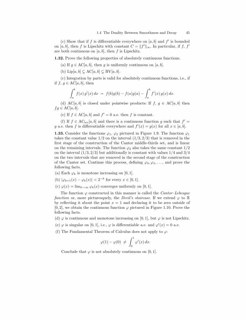
1.4 The Duality Between Smoothness and Decay 45
(c) Show that if f is differentiable everywhere on [a, b] and f ′ is boundedon [a, b], then f is Lipschitz with constant C = ‖f ′‖∞. In particular, if f, f ′
are both continuous on [a, b], then f is Lipschitz.
1.32. Prove the following properties of absolutely continuous functions.
(a) If g ∈ AC[a, b], then g is uniformly continuous on [a, b].
(b) Lip[a, b] ( AC[a, b] ( BV[a, b].
(c) Integration by parts is valid for absolutely continuous functions, i.e., ifif f, g ∈ AC[a, b], then
∫ b
a
f(x) g′(x) dx = f(b)g(b) − f(a)g(a) −∫ b
a
f ′(x) g(x) dx.
(d) AC[a, b] is closed under pointwise products: If f, g ∈ AC[a, b] thenfg ∈ AC[a, b].
(e) If f ∈ AC[a, b] and f ′ = 0 a.e. then f is constant.
(f) If f ∈ ACloc[a, b] and there is a continuous function g such that f ′ =g a.e. then f is differentiable everywhere and f ′(x) = g(x) for all x ∈ [a, b].
1.33. Consider the functions ϕ1, ϕ2 pictured in Figure 1.9. The function ϕ1
takes the constant value 1/2 on the interval (1/3, 2/3) that is removed in thefirst stage of the construction of the Cantor middle-thirds set, and is linearon the remaining intervals. The function ϕ2 also takes the same constant 1/2on the interval (1/3, 2/3) but additionally is constant with values 1/4 and 3/4on the two intervals that are removed in the second stage of the constructionof the Cantor set. Continue this process, defining ϕ3, ϕ4, . . . , and prove thefollowing facts.
(a) Each ϕk is monotone increasing on [0, 1].
(b) |ϕk+1(x) − ϕk(x)| < 2−k for every x ∈ [0, 1].
(c) ϕ(x) = limk→∞ ϕk(x) converges uniformly on [0, 1].
The function ϕ constructed in this manner is called the Cantor–Lebesguefunction or, more picturesquely, the Devil’s staircase. If we extend ϕ to R
by reflecting it about the point x = 1 and declaring it to be zero outside of[0, 2], we obtain the continuous function ϕ pictured in Figure 1.10. Prove thefollowing facts.
(d) ϕ is continuous and monotone increasing on [0, 1], but ϕ is not Lipschitz.
(e) ϕ is singular on [0, 1], i.e., ϕ is differentiable a.e. and ϕ′(x) = 0 a.e.
(f) The Fundamental Theorem of Calculus does not apply to ϕ:
ϕ(1) − ϕ(0) 6=∫ 1
0
ϕ′(x) dx.
Conclude that ϕ is not absolutely continuous on [0, 1].
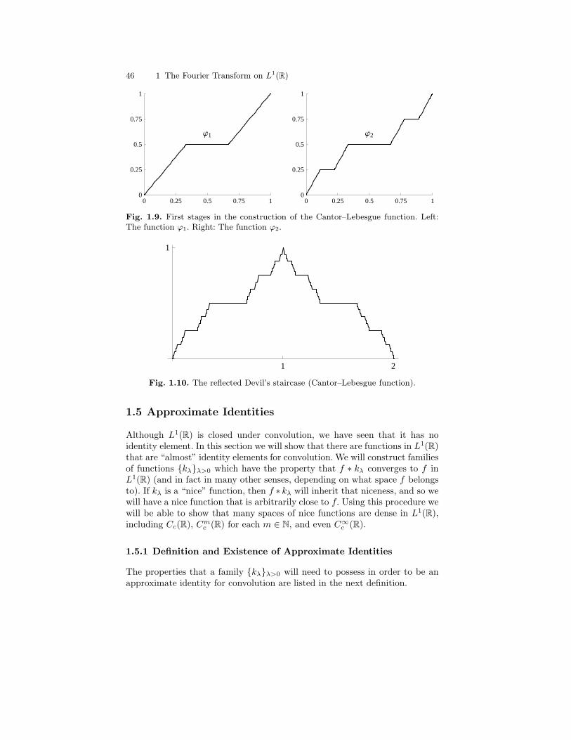
46 1 The Fourier Transform on L1(R)
j1
0 0.25 0.5 0.75 10
0.25
0.5
0.75
1
j2
0 0.25 0.5 0.75 10
0.25
0.5
0.75
1
Fig. 1.9. First stages in the construction of the Cantor–Lebesgue function. Left:The function ϕ1. Right: The function ϕ2.
1 2
1
Fig. 1.10. The reflected Devil’s staircase (Cantor–Lebesgue function).
1.5 Approximate Identities
Although L1(R) is closed under convolution, we have seen that it has noidentity element. In this section we will show that there are functions in L1(R)that are “almost” identity elements for convolution. We will construct familiesof functions kλλ>0 which have the property that f ∗ kλ converges to f inL1(R) (and in fact in many other senses, depending on what space f belongsto). If kλ is a “nice” function, then f ∗ kλ will inherit that niceness, and so wewill have a nice function that is arbitrarily close to f. Using this procedure wewill be able to show that many spaces of nice functions are dense in L1(R),including Cc(R), Cm
c (R) for each m ∈ N, and even C∞c (R).
1.5.1 Definition and Existence of Approximate Identities
The properties that a family kλλ>0 will need to possess in order to be anapproximate identity for convolution are listed in the next definition.

1.5 Approximate Identities 47
Definition 1.69. An approximate identity or a summability kernel is a familykλλ>0 of functions in L1(R) satisfying
(a) Normalization:∫
kλ(x) dx = 1 for every λ > 0,
(b) L1-boundedness : supλ ‖kλ‖1 < ∞, and
(c) L1-concentration: For every δ > 0,
limλ→∞
∫
|x|≥δ
|kλ(x)| dx = 0. ♦
By definition, an approximate identity is a family of integrable functions.If it is the case that kλ ≥ 0 for each λ, then requirement (b) in Definition 1.69follows from requirement (a). However, in general the elements of an approx-imate identity need not be nonnegative functions.
The “easy” way to create an approximate identity is through dilation of asingle function.
Exercise 1.70. Let k ∈ L1(R) be any function that satisfies
∫k(x) dx = 1.
Define kλ by an L1-normalized dilation:
kλ(x) = λk(λx), λ > 0,
and show that the family kλλ>0 forms an approximate identity. ♦
Note that there is an inherent ambiguity in our notation: We may usekλλ>0 to indicate a generic family of functions indexed by λ, or, as intro-duced in Notation 1.5, we may use kλ to denote the L1-normalized dilationof a function k. The intended meaning is usually clear from context.
In any case, if we define kλ by dilation, then, as λ increases, kλ becomesmore and more similar to our intuition of what a “δ-function” (a function thatis an identity for convolution) would look like (see the illustration in Figure 1.7and the related discussion in Section 1.3.5). While there is no such identity forconvolution in L1(R), the collection of functions kλλ>0 in some sense formsan approximation to this nonexistent δ-function, for requirement (c) impliesthat kλ becomes more and more concentrated near the origin as λ increases,with
∫kλ = 1 for every λ.
Consider also the appearance of kλ(x) = λk(λx) in the frequency domain.By Exercise 1.13, we have
kλ(ξ) = k
(ξ
λ
).
Since k is integrable with∫
k = 1, we know that k is continuous, and

48 1 The Fourier Transform on L1(R)
k(0) =
∫k = 1.
The continuity of k therefore implies that for each ξ ∈ R we have
limλ→∞
kλ(ξ) = limλ→∞
k
(ξ
λ
)= k(0) = 1 (1.25)
(see the illustration in Figure 1.11 using the Gaussian function g(x) = e−πx2
,
which by Exercise 1.109 has the interesting property that g(ξ) = e−πξ2
). Thus
kλ converges pointwise everywhere to the constant function 1. This againmatches our intuition for what the Fourier transform of a “δ-function” wouldbe if there was one, for if there was a function δ that satisfied both δ(x) = 0
for x 6= 0 and∫
δ = 1, then δ would be identically constant:
δ(ξ) =
∫δ(x) e−2πiξx dx =
∫δ(x) dx = 1.
This contradicts the Riemann–Lebesgue Lemma, so no such function δ canexist. However, when we define δ not as a function but rather as a distributionin Chapter 4 or as a measure in Chapter 5, we will see that δ does exist andis precisely the constant function.
In any case, given any f ∈ L1(R) and an approximate identity kλλ>0 ofthe form kλ(x) = λk(λx), we have that
(f ∗ kλ)∧
(ξ) = f(ξ) kλ(ξ) → f(ξ), ξ ∈ R.
So, we at least have that (f ∗ kλ)∧
(ξ) converges pointwise to f(ξ), and thisgives us hope that f ∗ kλ should converge to f in other senses as well. Ourgoal in this section is understand in what sense this hope holds true.
1.5.2 Approximation in Lp(R) by an Approximate Identity
We begin by quantifying the notion that an approximate identity is approxi-mately an identity for convolution in L1(R). The proof of this theorem illus-trates the “standard trick” of introducing kλ into an equation by virtue ofthe fact that
∫kλ = 1, and also the division of the integral into small and
large parts in order to make use of the defining properties of an approximateidentity.
Theorem 1.71. Let kλλ>0 be an approximate identity. Then
∀ f ∈ L1(R), limλ→∞
‖f − f ∗ kλ‖1 = 0.
That is, f ∗ kλ → f in L1-norm as λ → ∞.

1.5 Approximate Identities 49
-5 -4 -3 -2 -1 0 1 2 3 4 5
1
-5 -4 -3 -2 -1 0 1 2 3 4 5
1
-5 -4 -3 -2 -1 0 1 2 3 4 5
1
Fig. 1.11. Top: The Fourier transform bg(ξ) = e−πξ2
of the function g(x) = e−πx2
.Middle: The Fourier transform bg5(ξ) = bg(ξ/5) of the dilated function g5(x) = 5g(5x).Bottom: The Fourier transform cg15(ξ) = bg(ξ/15) of the dilated function g15(x) =15g(15x).
Proof. Fix any f ∈ L1(R). Since kλ ∈ L1(R), we know that f ∗ kλ ∈ L1(R),and we wish to show that it approximates f well in L1-norm. Using the factthat
∫kλ = 1, we compute that
50 1 The Fourier Transform on L1(R)
‖f − f ∗ kλ‖1 =
∫|f(x) − (f ∗ kλ)(x)| dx
=
∫ ∣∣∣∣f(x)
∫kλ(t) dt −
∫f(x − t) kλ(t) dt
∣∣∣∣ dx
≤∫∫
|f(x) − f(x − t)| |kλ(t)| dt dx
=
∫∫|f(x) − f(x − t)| |kλ(t)| dx dt
=
∫|kλ(t)|
∫|f(x) − Ttf(x)| dx dt
=
∫|kλ(t)| ‖f − Ttf‖1 dt, (1.26)
where the interchange in the order of integration is permitted by Tonelli’sTheorem since the integrands are nonnegative. We want to show that thequantity in equation (1.26) is small when λ is large.
Choose any ε > 0. Since translation is strongly continuous on L1(R), thereexists a δ > 0 such that
|t| < δ =⇒ ‖f − Ttf‖1 < ε.
Also, by definition of approximate identity, we know that
K = supλ
‖kλ‖1 < ∞,
and that there exists some λ0 such that
λ > λ0 =⇒∫
|t|≥δ
|kλ(t)| dt < ε.
Therefore, for λ > λ0 we can continue equation (1.26) as follows:
(1.26) =
∫
|t|<δ
|kλ(t)| ‖f − Ttf‖1 dt +
∫
|t|≥δ
|kλ(t)| ‖f − Ttf‖1 dt
≤∫
|t|<δ
|kλ(t)| ε dt +
∫
|t|≥δ
|kλ(t)|(‖f‖1 + ‖Ttf‖1
)dt
≤ ε
∫|kλ(t)| + 2‖f‖1
∫
|t|≥δ
|kλ(t)| dt
≤ εK + 2‖f‖1 ε.
Thus ‖f − f ∗ kλ‖1 → 0 as λ → ∞. ⊓⊔
To illustrate the convergence proved in the preceding theorem, considerthe particular function χ = χ[0,1] and a particular approximate identity that

1.5 Approximate Identities 51
will be of considerable use to us later. This is the Fejer kernel wλλ>0,
which is produced by dilating the Fejer function w(x) =(
sin πxπx
)2depicted in
Figure 1.14. In Figure 1.12, we see the convolutions χ∗w, χ∗w5, and χ∗w25. Inaddition to the convergence apparent in these figures, note that the convolvedfunctions appear to be continuous, while χ is discontinuous. This is due tothe smoothing effect of convolution, which was discussed in Section 1.3.7.
-1.0 -0.5 0.5 1.0 1.5 2.0-0.2
0.2
0.4
0.6
0.8
1.0
-1.0 -0.5 0.5 1.0 1.5 2.0-0.2
0.2
0.4
0.6
0.8
1.0
-1.0 -0.5 0.5 1.0 1.5 2.0-0.2
0.2
0.4
0.6
0.8
1.0
Fig. 1.12. Convolution with an approximate identity. Top: χ ∗ w. Middle: χ ∗ w5.Bottom: χ ∗ w25.
There are many variations on the theme of Theorem 1.71. To begin, sinceLp ∗ L1 ⊆ Lp, we expect that we may be able to extend to other values of p,and indeed for p finite we have the following result.

52 1 The Fourier Transform on L1(R)
Exercise 1.72. Let kλλ>0 be an approximate identity. Prove that if 1 ≤p < ∞, then
∀ f ∈ Lp(R), limλ→∞
‖f − f ∗ kλ‖p = 0.
That is, f ∗ kλ → f in Lp-norm as λ → ∞. ♦
As usual, we do need to be careful when p = ∞, and we consider this issuenext.
1.5.3 Uniform Convergence
Now we turn to approximation by approximate identities in spaces such asL∞(R), C0(R), and Cb(R). Considering that the elements kλ of an approx-imate identity are integrable functions, if f belongs to L∞(R) then f ∗ kλ
belongs to Cb(R) by Exercise 1.39. Hence it is simply too much to expectthat f ∗ kλ will converge to f in L∞-norm for all f ∈ L∞(R). However, if weimpose some smoothness on f, then we can obtain convergence in senses thatare appropriate to f.
If we assume that f belongs to C0(R), then f ∗ kλ also belongs to C0(R)by Theorem 1.36. By replacing L∞(R) with C0(R), we therefore obtain forp = ∞ an exact analogue of the convergence result of Exercise 1.72.
Exercise 1.73. Let kλλ>0 be an approximate identity. Prove that
∀ f ∈ C0(R), limλ→∞
‖f − f ∗ kλ‖∞ = 0.
That is, f ∗ kλ converges uniformly to f as λ → ∞. ♦
Suppose that we relax the decay hypothesis on f in Exercise 1.73, andassume only that f ∈ Cb(R) instead of in C0(R). In this case we do have thatf ∗ kλ ∈ Cb(R) by Exercise 1.39, so we can hope that f ∗ kλ will still convergeto f. This is true, but in general the convergence will be uniform only whenrestricted to compact sets.
Exercise 1.74. Let kλλ>0 be an approximate identity. Prove that if f ∈Cb(R), then f ∗ kλ converges uniformly to f on compact sets, i.e.,
∀ compact K ⊆ R, limλ→∞
∥∥(f − f ∗ kλ)χK
∥∥∞
= 0.
Give an example of f ∈ Cb(R) such that f ∗ kλ does not converge uniformlyto f on R. ♦
On the other hand, if we impose even a slight amount of “extra smooth-ness” on f ∈ Cb(R), then we can restore the uniform convergence of f ∗ kλ
to f on the entire real line. We can quantify this extra smoothness in termsof Holder continuity, which is a generalization of Lipschitz continuity.
1.5 Approximate Identities 53
Definition 1.75. (a) A function f : R → C is Holder continuous with expo-nent α > 0 at a point x if there exists a constant K > 0 such that
∀ y ∈ R, |f(x) − f(y)| ≤ K |x − y|α.
(b) f is Holder continuous with exponent α > 0 if there exists a constantK > 0 such that
∀x, y ∈ R, |f(x) − f(y)| ≤ K |x − y|α.
(c) Given 0 < α < 1, we set
Cα(R) =f ∈ C(R) : f is Holder continuous with exponent α
. ♦
The reader should verify that the only functions that are Holder contin-uous with exponent α > 1 are the constant functions. Lipschitz continuityis Holder continuity with α = 1. Every differentiable function f such thatf ′ is bounded is Lipschitz, but a Lipschitz function need not be differentiableeverywhere (consider f(x) = |x|). Hence C1(R), the space of function that aredifferentiable with a continuous derivative, is a proper subspace of the spaceof Lipschitz functions. A Lipschitz function f has bounded variation on anyfinite interval, and consequently f is differentiable at almost every point andf ′ is integrable on any finite interval.
The graph of a function that is Holder continuous with exponent α < 1typically has a “fractal” appearance. The smaller that we must take α, themore “jagged” the graph of the function appears. For example, the Cantor–Lebesgue function is Holder continuous but not Lipschitz (Problem 1.42).
Exercise 1.76. Let kλλ>0 be an approximate identity. Prove that if f ∈Cb(R) is Holder continuous for some exponent 0 < α ≤ 1, then f ∗kλ convergesuniformly to f on R, i.e.,
limλ→∞
‖f − f ∗ kλ‖∞ = 0. ♦
1.5.4 Pointwise Convergence
If f is a locally integrable function, then x ∈ R is a Lebesgue point of f if
limh→0
1
2h
∫ x+h
x−h
|f(y) − f(x)| dy = 0,
and the set of Lebesgue points is called the Lebesgue set of f. Every pointof continuity is a Lebesgue point of f. More interestingly, the Lebesgue Dif-ferentiation Theorem implies that almost every x ∈ R is a Lebesgue point(Theorem A.30).
Now, we have seen that if f belongs to Lp(R) with p finite then f ∗kλ → fin Lp-norm. If we impose some restrictions on k, then we can also show thatwe have pointwise convergence of (f ∗kλ)(x) to f(x) at each Lebesgue point xof f.

54 1 The Fourier Transform on L1(R)
Theorem 1.77. Let k be a bounded, compactly supported function such that∫k = 1, and define kλ(x) = λk(λx). If f ∈ L1(R), then (f ∗ kλ)(x) → f(x)
as λ → ∞ for each point x in the Lebesgue set of f. In particular, f ∗ kλ
converges to f pointwise a.e.
Proof. By hypothesis, supp(k) ⊆ [−R, R] for some R. If x is a Lebesgue pointof f, then
limλ→∞
|f(x) − (f ∗ kλ)(x)|
= limλ→∞
∣∣∣∣f(x)
∫kλ(x − t) dt −
∫f(t) kλ(x − t) dt
∣∣∣∣
≤ limλ→∞
λ
∫|f(x) − f(t)| |k(λ(x − t))| dt
= limλ→∞
2Rλ
2R
∫ x+(R/λ)
x−(R/λ)
|f(x) − f(t)| |k(λ(x − t))| dt
≤ 2R ‖k‖∞ limh→0
1
2h
∫ x+h
x−h
|f(x) − f(t)| dt
= 0,
where the limit is zero by definition of Lebesgue point. Finally, since almostevery x is a Lebesgue point of f, we conclude that f ∗ kλ converges to fpointwise a.e. ⊓⊔
The hypotheses on k in Theorem 1.77 can be relaxed. In particular, com-pact support of k is not required. For example, Stein and Weiss [SW71, p. 13]give a more intricate argument that shows that if k ∈ L1(R) satisfies
∫k = 1
and there exists an even function φ ∈ L1(R) that is decreasing and differen-tiable on (0,∞) that dominates k in the sense that |k(x)| ≤ φ(x) for all x,then (f ∗ kλ)(x) → f(x) for every x in the Lebesgue set of f.
1.5.5 Dense Sets of Nice Functions
Theorem 1.16 gave us a proof, based on Urysohn’s Lemma, that the spaceCc(R) is dense in L1(R). It almost seems that we should be able to give a“simple” proof of this fact by using approximate identities and arguing asfollows. Choose any f ∈ L1(R). Then we can find a compactly supported g ∈L1(R) that is close to f, e.g., if we take R large enough and set g = f χ[−R,R]
then we will have ‖f − g‖1 < ε. If we convolve g with an element kλ of anapproximate identity, then g ∗ kλ will be close to g if λ is large enough, say‖g− g ∗ kλ‖1 < ε. Further, if we choose our approximate identity so that kλ isa “nice” function then g ∗ kλ will inherit this “niceness” as well. For example,if kλ ∈ Cc(R) then g ∗ kλ ∈ Cc(R), and so we have found an element of Cc(R)that lies within 2ε of f in L1-norm.

1.5 Approximate Identities 55
The flaw in this reasoning is that our proof in Theorem 1.71 that g∗kλ → gin L1-norm relies on the fact that translation is a strongly continuous familyof operators in L1(R). The proof of this strong continuity of translation isthe content of Exercise 1.17. However, the proof of that exercise (at least theproof we suggest in the hints) requires us to already know that Cc(R) is densein L1(R). Hence the reasoning of the preceding paragraph is circular.
We could take a different approach, e.g., by first arguing that simple func-tions are dense in L1(R) and trying to proceed from there to show that Cc(R)is dense. But it doesn’t really matter, one way or the other we essentiallyhave to “get our hands dirty” and show that some particular special subset isdense. The power of approximate identities comes at the next step—once weknow that one particular set is dense, we can use the spirit of the argumentabove (convolution with a “nice” approximate identity) to easily show that“much nicer” spaces are also dense. We even obtain results that almost seemtoo good to be true. For example, we will see that the space C∞
c (R) consistingof infinitely differentiable, compactly supported functions is dense in Lp(R) forevery 1 ≤ p < ∞! This fact is not just an abstract surprise, but will be ofgreat utility to us throughout the remainder of this volume, especially whenwe turn to distribution theory in Chapter 4.
Exercise 1.78. (a) Show that Cmc (R) is dense in Lp(R) for each m ≥ 0 and
1 ≤ p < ∞, and also is dense in C0(R) in L∞-norm.
(b) Show that C∞c (R) is dense in Lp(R) for each 1 ≤ p < ∞, and also is
dense in C0(R) in L∞-norm. ♦
After proving the Inversion Formula in Section 1.6, we will also be ableto show that many spaces of functions with nice Fourier transforms are alsodense. For example, in Problem 1.66 we will see that
f ∈ L1(R) : f ∈
C∞c (R)
is dense in Lp(R) for 1 ≤ p < ∞.
1.5.6 The C∞ Urysohn Lemma
We proved Urysohn’s Lemma for the setting of the real line in Theorem 1.15.By using approximate identities, we now prove a much more refined C∞-version of Urysohn’s Lemma for subsets of R.
Theorem 1.79 (C∞ Urysohn Lemma). Let K ⊆ R be compact, and letU ⊇ K be an open set. Then there exists f ∈ C∞
c (R) such that 0 ≤ f ≤ 1,f = 1 on K, and supp(f) ⊆ U.
Proof. Since K is compact and R\U is closed, the distance between these setsis positive, i.e.,
d = dist(K, R\U) = inf|x − y| : x ∈ K, y /∈ U
> 0.
Let
56 1 The Fourier Transform on L1(R)
V =y ∈ R : dist(y, K) <
d
3
,
and let k be any function in C∞c (R) such that k ≥ 0,
∫k = 1, and supp(k) ⊆
[− d3 , d
3 ] (for example, dilate the function constructed in Exercise 1.42). Set
f = k ∗ χV . Since k and χV are both compactly supported, their convolutionis also compactly supported, and hence it follows from Corollary 1.41 thatf ∈ C∞
c (R). Since
f(x) =
∫
V
k(x − y) dy ≤∫
k = 1,
we have 0 ≤ f ≤ 1 everywhere. Also, if x ∈ K and y /∈ V then |x − y| ≥ d3
and so k(x − y) = 0. Therefore for x ∈ K we have
f(x) =
∫
V
k(x − y) dy =
∫k(x − y) dy = 1.
Similarly if x /∈ U then it follows that f(x) = 0. ⊓⊔
1.5.7 Gibbs’s Phenomenon
Gibbs’s phenomenon refers to the behavior of the partial sums of the Fourierseries of a periodic function near a jump discontinuity. Although this chapterfocuses on the Fourier transform on R rather than Fourier series on T, thereis an analogous phenomenon for the Fourier transform that we will discuss.For the formulation and proof of Gibbs’s phenomenon on the torus, we referto [DM72].
To illustrate this, let H = χ[0,∞) be the Heaviside function. AlthoughH does not belong to L1(R), the important fact for this example is that Hhas a jump discontinuity at x = 0. Pointwise convergence of Fourier seriescorresponds to convolution with the Dirichlet kernel on the torus (see Sec-tion 2.2.1, and equation (2.9) in particular). The Dirichlet kernel on the realline is dλλ>0, which is obtained by dilating the Dirichlet function
d(ξ) =sin ξ
πξ.
Since d /∈ L1(R), the Dirichlet kernel does not form an approximate identity,but even so let us consider the pointwise behavior of H ∗ dλ as λ → ∞.
Using the fact that, as an improper Riemann integral,∫ ∞
0sin x
x dx = π2 (see
Problem 1.43), we have
(H ∗ dλ)(x) =
∫ ∞
0
sinλ(x − y)
π(x − y)dy
=
∫ λx
−∞
sin y
πydy

1.5 Approximate Identities 57
=1
2+
∫ λx
0
sin y
πydy.
Since sin yπy > 0 for 0 < y < π, H ∗ dλ is increasing on (0, π/λ). Then it
decreases on (π/λ, 2π/λ), then increases on (2π/λ, 3π/λ)—but never back tothe value it had at π/λ. Continuing in this way we see that H ∗ dλ achievesits maximum at x = π/λ, and this maximum is
(H ∗ dλ)(π
λ
)=
1
2+
∫ π
0
sin y
πydy ≈ 1.089 . . . .
Note that this maximum is independent of λ. Although (H ∗ dλ)(x) convergespointwise to H(x) as λ → ∞ for all x 6= 0, this convergence is not uniform.In particular, the maximum distance between (H ∗dλ)(x) and H(x) for x > 0is a constant (approximately 0.089. . . ) that is independent of λ, although itslocation at x = π/λ decreases with λ. Figure 1.13 displays a plot of H ∗ dλ
for λ = 16π.
-0.4 -0.2 0.2 0.4
0.2
0.4
0.6
0.8
1.0
Fig. 1.13. Graph of H ∗ dλ for λ = 16π.
1.5.8 Translation-Invariant Subspaces of L1(R)
The following characterization of the closed, translation-invariant subspacesof L1(R) is due to Norbert Wiener (1894–1964); compare this to the char-acterization of the closed, translation-invariant subspaces of L2(R) given inProblem 3.10.
Definition 1.80 (Translation-Invariant Subspaces). We say that a sub-set J of L1(R) is translation-invariant if J is closed under all translations,i.e., if
f ∈ J, a ∈ R =⇒ Taf ∈ J. ♦
58 1 The Fourier Transform on L1(R)
Remark 1.81. A shift-invariant space V is one that is closed under integertranslations, i.e., if f ∈ V then Tkf ∈ V for all integer k. These spaces playimportant roles in sampling theory and wavelet theory, see [Dau92]. ♦
Exercise 1.82. Let J be a closed subspace of L1(R), and prove that thefollowing statements are equivalent.
(a) J is translation-invariant.
(b) J is an ideal in L1(R) under convolution. ♦
Note that closedness is important here. For example, Cc(R) is a translation-invariant subspace of L1(R), but it is not an ideal with respect to convolution.
By using Exercise 1.82, we can give another characterization of the princi-
pal ideal I(g) = g ∗ L1(R) generated by a function g ∈ L1(R). By Exercise 1.48and Problem 1.39, I(g) is the smallest closed ideal in L1(R) that contains g.
Exercise 1.83. Given g ∈ L1(R), show that I(g) is the closure of the finitelinear span of the translations of g:
I(g) = span(Taga∈R
). ♦
Thus, the smallest closed ideal that contains g is precisely the smallestclosed subspace that contains all translates of g.
Recall that a set S ⊆ L1(R) is complete in L1(R) if span(S) is dense inL1(R). It therefore follows from Exercise 1.83 that Taga∈R is complete inL1(R) if and only if I(g) = L1(R). But when does this happen? The nextexercise gives a necessary condition.
Exercise 1.84. Given g ∈ L1(R), show that
Taga∈R is complete in L1(R) =⇒ g(ξ) 6= 0 for all ξ ∈ R. ♦
The converse of Exercise 1.84 is also true, but is a much deeper fact thatis part of Wiener’s Tauberian Theorem, which we discuss in Section 2.10. Incontrast, the analogous question in L2(R) is much simpler, see Problem 3.9.
Additional Problems
1.34. This problem constructs an example of an approximate identity kλλ>0
where kλ need not be a dilation of a single function k. For each λ > 0,let kλ ∈ L1(R) be any function satisfying kλ ≥ 0, ‖kλ‖1 =
∫kλ = 1, and
supp(kλ) ⊆ [− 1λ , 1
λ ]. Show that kλλ>0 is an approximate identity.
1.35. Show that if kλλ>0 is an approximate identity then kλ(ξ) → 1 point-wise as λ → ∞.
1.36. Let kλλ>0 be an approximate identity and fix f ∈ L1(R) ∩ L∞(R).Show that if f is continuous at some point x ∈ R, then (f ∗ kλ)(x) → f(x) asλ → ∞.
1.5 Approximate Identities 59
1.37. Fix g ∈ L1(R) and define Lg : L1(R) → L1(R) by Lg(f) = f ∗ g. Showthat the operator norm of Lg is ‖Lg‖ = ‖g‖1. This gives the best constant inequation (1.15) for the case p = q = r = 1.
1.38. Assume k ∈ L1(R) is given and we set r =∫
k and kλ(x) = λk(λx).Prove that if 1 ≤ p < ∞, then for each f ∈ Lp(R) we have that f ∗ kλ → rfin Lp-norm as λ → ∞. Note that this includes the possibility that r may becomplex or zero.
1.39. Fix g ∈ L1(R), and consider the ideals g ∗ L1(R) and I(g) introducedin Exercise 1.48. Show that we need not have g ∈ g ∗ L1(R), but we alwayshave g ∈ I(g).
1.40. Let k ∈ L1(R) be any function such that∫
k = 1 and xk(x) ∈ L1(R),and define an approximate identity by setting kλ(x) = λk(λx). Fix 1 ≤ p < ∞.
(a) Show that ‖Pkλ‖1 → 0 as λ → ∞, where P is the position operator.
(b) Show that if f ∈ Lp(R) then f ∗ Pkλ → 0 in Lp-norm. Further, if we alsohave xf(x) ∈ Lp(R), then P (f ∗ kλ) → Pf in Lp-norm.
1.41. Given 0 < α < 1, let Cα(R) be the space of Holder continuous functionsgiven in Definition 1.75. Show that
‖f‖Cα = |f(0)| + supx 6=y
f(x) − f(y)
|x − y|α
is a norm on Cα(R), and Cα(R) is complete with respect to this norm.
1.42. Show that the Cantor–Lebesgue function is Holder continuous preciselyfor exponents α in the range 0 < α ≤ log3 2 ≈ 0.6309 . . . .
1.43. (a) Show that∫ ∞
0
∣∣ sin xx
∣∣ dx = ∞.
(b) If x > 0, then∫ ∞
0 e−tx dt = 1x . Combine this with Fubini’s Theorem to
evaluate∫ a
0sin x
x dx. Then apply the Lebesgue Dominated Convergence The-
orem to show that lima→∞
∫ a
0sin x
x dx = π2 .
Thus, even though sin xx is not integrable, the improper Riemann integral∫ ∞
0sin x
x dx exists and equals π2 (this integral can also be evaluated by using
contour integration).
(c) Show that supa<b
∣∣∫ b
asin x
x dx∣∣ < ∞.
1.44. This problem will illustrate one of the many different possible gener-alizations of the results of this section by considering particular weighted Lp
spaces. Given s ∈ R let vs(x) = (1+|x|)s; we refer to vs as a polynomial weight(since it has polynomial-like growth if s ≥ 0, or decays like the reciprocal ofa polynomial if s ≤ 0). For this problem fix 1 ≤ p < ∞ and s ∈ R. Then wedefine Lp
s(R) to be the space of all measurable functions f : R → C such that
60 1 The Fourier Transform on L1(R)
‖f‖p,s = ‖f vs‖p =
(∫|f(x)|p (1 + |x|)ps dx
)1/p
< ∞.
If we identify functions that are equal a.e. then Lps(R) is a Banach space.
Prove the following statements.
(a) If s ≥ 0 then vs is submultiplicative, i.e., vs(x + y) ≤ vs(x) vs(y) forx, y ∈ R. If s ≤ 0 then vs is v−s-moderate, i.e., vs(x + y) ≤ vs(x) v−s(y) forx, y ∈ R.
(b) For each a ∈ R, the translation operator Ta is a continuous map ofLp
s(R) into itself, with operator norm ‖Ta‖Lps→Lp
s≤ v|s|(a) = (1 + |a|)|s|.
(c) Translation is strongly continuous on Lps(R), i.e., for each f ∈ Lp
s(R)we have lima→0 ‖f − Taf‖p,s = 0.
(d) If kλλ>0 is an approximate identity, then for each f ∈ Lps(R) we
have limλ→∞ ‖f − f ∗ kλ‖p,s = 0.
(e) C∞c (R) is dense in Lp
s(R).
(f) Do parts (b)–(d) still hold if we replace vs by an arbitrary weightw : R → (0,∞)? What properties do we need w to possess?
1.6 The Inversion Formula
In this section we will prove Theorem 1.9, the Inversion Formula for the Fouriertransform on L1(R), which states that if f and f both belong to L1(R), then
f =(f
)∨=
( ∨
f)∧
.Unfortunately, the Inversion Formula does not apply to every function in
L1(R). For example, by Exercise 1.7 we have that χ = χ[−1/2,1/2] belongs to
L1(R) but χ(ξ) = dπ(ξ) = sin πξπξ is not integrable. Another example is given
in Problem 1.1: The one-sided exponential function f(x) = e−x χ[0,∞)(x) is
integrable, but its Fourier transform f(ξ) = 12πiξ+1 is not.
1.6.1 The Fejer Kernel
To prove the Inversion Formula, we will use the machinery of approximateidentities that we developed in Section 1.5. Specifically, we will use a particularapproximate identity, named after Lipot Fejer (1880–1959), that has someuseful special properties.
Definition 1.85 (Fejer Kernel). The Fejer function is the square of thesinc function dπ:
w(x) =
(sinπx
πx
)2
= dπ(x)2.
The Fejer kernel is wλλ>0 where wλ(x) = λw(λx). ♦

1.6 The Inversion Formula 61
-4 -2 2 4-0.2
0.2
0.4
0.6
0.8
1.0
Fig. 1.14. Graph of the Fejer function w.
The letter “w” is for “Weiss,” which was Fejer’s surname at birth.In order to conclude that the Fejer kernel is an approximate identity, we
need to know that the integral of w is 1.
Exercise 1.86. Show that w ∈ L1(R) and∫
w = 1. ♦
Let χ = χ[−1/2,1/2]. Then we know from Exercise 1.7 that χ(ξ) = sin πξπξ =
dπ(ξ). Hence if we letW = χ ∗ χ,
then we haveW = χ 2
= d 2π = w. (1.27)
Also∨
W = w since W is even. Since both W and W = w belong to L1(R), ifwe had already proved that the Inversion Formula holds, then we could applyit to W to conclude that w’s Fourier transform is W, i.e.,
w = (∨
W )∧
= W and∨
w = (W)∨
= W. (1.28)
We will see eventually that this is true, but first we must prove the InversionFormula. And we will prove the Inversion Formula by making use of the Fejerkernel, although we will not need equation (1.28) to do this. Obviously, thisis a good thing, since otherwise the argument would be circular.
It is not so much the Fejer kernel itself that will be important to us, butrather some of the properties that it happens to have, including:
(a) w, W ≥ 0,
(b) w(0) = 1,
(c) W, W ∈ L1(R),
(d)∫
W = W(0) = 1.
Even these are not all essential, and the reader can consider what other kernelswe might use instead to prove the Inversion Formula.

62 1 The Fourier Transform on L1(R)
-1.5 -1.0 -0.5 0.0 0.5 1.0 1.5
0.2
0.4
0.6
0.8
1.0
Fig. 1.15. Graph of the hat function W.
Exercise 1.87. Prove that W is the hat function or tent function on theinterval [−1, 1] defined by
W (ξ) = max1 − |ξ|, 0. ♦
Consequently,
W (ξ/λ) = max1 − |ξ|
λ, 0
(1.29)
is the dilated hat function with height 1 supported on [−λ, λ]. In particular,W (ξ/λ) → 1 pointwise as λ → ∞.
1.6.2 Proof of the Inversion Formula
To motivate our first step towards the proof of the Inversion Formula, chooseany f ∈ L1(R). Then f ∗ wλ ∈ L1(R) and also (f ∗ wλ)
∧
= f wλ. We don’tknow this yet, but we will show that wλ(ξ) = W (ξ/λ) ∈ L1(R). Once we
establish this, it follows (since f is bounded) that
(f ∗ wλ)∧
= f wλ ∈ L1(R).
Hence, if only we already knew that the Inversion Formula was valid, we couldcompute that
(f ∗ wλ)(x) =((f ∗ wλ)
∧)∨
(x) = (f wλ)∨
(x) =
∫f(ξ)W (ξ/λ) e2πiξx dξ.
Unfortunately, these calculations are not yet justified since, among otherthings, they rely on the Inversion Formula, which has not yet been proved.However, instead of trying to justify the full Inversion Formula right now, webegin with a much smaller step: We show directly that the specific equality(f ∗ wλ)(x) =
∫f(ξ)W (ξ/λ) e2πiξx dξ holds when f ∈ L1(R).
Theorem 1.88. If f ∈ L1(R), then for each λ > 0 we have
1.6 The Inversion Formula 63
(f ∗ wλ)(x) =
∫f(ξ)W (ξ/λ) e2πiξx dξ
=
∫ λ
−λ
f(ξ)(1 − |ξ|
λ
)e2πiξx dξ. (1.30)
Proof. We already know that
w(x) =∨
W (x) =
∫W (ξ) e2πiξx dξ,
and therefore by making a change of variables it follows that
wλ(x) = λw(λx) =
∫W (ξ/λ) e2πiξx dξ.
Suppose that f ∈ L1(R) is given. Assuming for the moment that the use ofFubini’s Theorem in the following calculation is justified, we have that
(f ∗ wλ)(x) =
∫f(y)wλ(x − y) dy
=
∫f(y)
∫W (ξ/λ) e2πiξ(x−y) dξ dy
=
∫ ∫ λ
−λ
f(y)(1 − |ξ|
λ
)e2πiξ(x−y) dξ dy
=
∫ λ
−λ
(∫f(y) e2πiξ(x−y) dy
)(1 − |ξ|
λ
)dξ
=
∫ λ
−λ
f(ξ)(1 − |ξ|
λ
)e2πiξx dξ.
Of course, the applicability of Fubini’s Theorem does have to be justified, andwe assign this task to the reader as an exercise. ⊓⊔
Now we obtain the Inversion Formula by taking the limit in equation(1.30).
Theorem 1.89 (Inversion Formula). If f, f ∈ L1(R), then f and f arecontinuous, and
f(x) =(f
)∨(x) =
∫f(ξ) e2πiξx dξ, (1.31)
with equality holding pointwise everywhere, and similarly
f(x) =( ∨
f)∧
(x) =
∫∨
f (ξ) e−2πiξx dξ
for every x.

64 1 The Fourier Transform on L1(R)
Proof. Since f ∈ L1(R), we know that f is a continuous function on R. There-fore, for any fixed x, we have the pointwise limit
∀ ξ ∈ R, limλ→∞
f(ξ)W (ξ/λ) e2πiξx = f(ξ) e2πiξx.
Further, since 0 ≤ W ≤ 1,
|f(ξ)W (ξ/λ) e2πiξx| ≤ |f(ξ)| ∈ L1(R).
Since f ∗wλ is continuous by Theorem 1.36, it is defined pointwise everywhere.By Theorem 1.88 and the Lebesgue Dominated Convergence Theorem, wetherefore have for each x that
limλ→∞
(f ∗ wλ)(x) = limλ→∞
∫f(ξ)W (ξ/λ) e2πiξx dξ
=
∫f(ξ) e2πiξx dξ =
(f
)∨(x).
On the other hand, f ∗ wλ → f in L1-norm, so there is a subsequence such
that (f ∗ wλk)(x) → f(x) for almost every x. Therefore
(f
)∨(x) = f(x) a.e.
Since(f
)∨is continuous, by redefining f on a set of measure zero we can
assume that equality holds pointwise everywhere. ⊓⊔
Observe that the hypothesis f, f ∈ L1(R) can be equivalently restated as
f, f ∈ L1(R) ⇐⇒ f ∈ L1(R) ∩ A(R).
Corollary 1.90. If f, f ∈ L1(R), then f, f ∈ C0(R). ♦
One consequence of the Inversion Formula is that we can now justify ourhope, presented in equation (1.28), that w = W. Note that since w and W areeven, their Fourier and inverse Fourier transforms coincide.
Corollary 1.91. w = (∨
W )∧
= W = (W)∨
=∨
w.
Proof. This follows from the Inversion Formula, the fact that w and W both
belong to L1(R), and our proof in equation (1.27) that W = w. ⊓⊔
An additional consequence is that the Fourier transform is an injectivemap on L1(R).
Theorem 1.92 (Uniqueness Theorem). If f, g ∈ L1(R), then
f = g a.e. ⇐⇒ f = g a.e.
In particular,f = 0 a.e. ⇐⇒ f = 0 a.e.
1.6 The Inversion Formula 65
Proof. Since the Fourier transform is linear, the first equivalence is a con-
sequence of the second. If f = 0 a.e., then f = 0 everywhere by defini-
tion of the Fourier transform. On the other hand, if f = 0 a.e., then we
have both f, f ∈ L1(R), so the Inversion Formula applies, and we obtain
f =(f
)∨=
∨
0 = 0. ⊓⊔Note that we could also appeal to Theorem 1.88 to give another proof of
the Uniqueness Theorem.
1.6.3 Summability
If f /∈ L1(R) then the Inversion Formula need not hold. However, as animmediate consequence of Theorem 1.88, we have the following approximation
formula for f in terms of f that is valid for all f ∈ L1(R), even if f is notintegrable.
Theorem 1.93. If f ∈ L1(R), then
∫ λ
−λ
f(ξ)(1 − |ξ|
λ
)e2πiξx dξ → f in L1-norm as λ → ∞. (1.32)
Proof. Simply note that, by Theorem 1.88, the left-hand side of equation(1.32) is f ∗ wλ. ⊓⊔
Thus, even if f /∈ L1(R), we have an “approximate” interpretation of the
formula f =(f
)∨in the sense that equation (1.32) will hold. This is analogous
to using summability conditions for evaluating divergent series. For example,consider a formal1 bi-infinite series of the form
∑∞k=−∞ ak. Let us say that
this series converges and equals L if the symmetric partial sums
sN =
N∑
k=−N
ak
converge to L. The Cesaro means or arithmetic means of these partial sumsare
σN =s0 + s1 + · · · + sN
N + 1.
If the series∑∞
k=−∞ ak converges (for example, if a = (ak)k∈Z is a summablesequence), then the Cesaro means will converge to the same limit. However,the Cesaro means may converge even when the partial sums do not; if theCesaro means converge then we say that
∑∞k=−∞ ak is Cesaro summable.
Further, the form of the Cesaro means given in the next exercise suggests aninteresting analogy with Theorem 1.93.
1It is an amusing linguistic footnote that a formal statement in mathematicsmeans that the statement is entirely informal. In particular, we use the term “for-mal” at this point because the symbols
P∞
k=−∞ak denote a completely arbitrary
series, without any requirement that it converge in any sense whatsoever.

66 1 The Fourier Transform on L1(R)
Exercise 1.94. Given a sequence of scalars a = (ak)k∈Z, let the partial sumssN and Cesaro means σN be as above.
(a) Show that
σN =
N∑
k=−N
(1 − |k|
N + 1
)ak.
(b) Show that if the partial sums sN converge, then the Cesaro means σN
converge to the same limit, i.e.,
limN→∞
N∑
k=−N
(1 − |k|
N + 1
)ak = lim
N→∞sN =
∞∑
k=−∞
ak. (1.33)
(c) Set ak = (−1)k for k ≥ 0 and ak = 0 for k < 0. Show that the series∑
ak
is Cesaro summable even though the partial sums do not converge, andfind the limit of the Cesaro means.
(d) Show that if ak ≥ 0 for every k then σN converges if and only if sN
converges. ♦
Comparing Theorem 1.93 to equation (1.33), we see that Theorem 1.93 isa continuous version of Cesaro summability. Essentially, Theorem 1.93 saysthat if f ∈ L1(R), then the formal integral
(f
)∨(x) =
∫ ∞
−∞
f(ξ) e2πiξx dξ
is Cesaro summable to f even if f is not integrable.It is possible to make this analogy even more precise. Just as the integral
in equation (1.32) is related to the convolution of f with the Fejer kernel,specifically,
(f ∗ wλ)(x) = (f wλ)∨
(x) =
∫ λ
−λ
f(ξ)(1 − |ξ|
λ
)e2πiξx dξ,
it is also true that Cesaro means of an infinite series are related to a discreteversion of the Fejer kernel. Indeed, when comparing the Fourier transform toFourier series, the two Fejer kernels play entirely analogous roles. We expandon this in Section 2.2.
As an application, we use Theorem 1.93 to obtain useful results regard-ing functions with compactly supported Fourier transforms. Such functionsappear in a variety of contexts. For example, we will see them again in Chap-ter 3 when we prove the Paley–Wiener Theorem (Section 3.5) and the energyconcentration theorems (Section 3.8).
Definition 1.95 (Bandlimited Function). We say that a function f is
bandlimited if supp(f ) is compact. ♦
1.6 The Inversion Formula 67
Exercise 1.96. (a) Show that the space of bandlimited functions in L1(R),
f ∈ L1(R) : supp(f ) is compact,
is dense in L1(R).
(b) Show that if Ω is fixed, then the space of functions in L1(R) bandlim-ited to [−Ω, Ω],
f ∈ L1(R) : supp(f ) ⊆ [−Ω, Ω],is a closed proper subspace of L1(R). ♦
1.6.4 Pointwise Inversion
As we have seen, the Cesaro means σN of a formal infinite series may convergeeven when the partial sums sN do not. For the Fourier transform, the analogueof the Cesaro means are convolutions with the Fejer kernel:
(f ∗ wλ)(x) =
∫ λ
−λ
f(ξ)(1 − |ξ|
λ
)e2πiξx dξ.
We always have f ∗ wλ → f in L1-norm when f ∈ L1(R).Similarly, the analogue of the partial sums for the Fourier transform are
convolutions with the Dirichlet kernel. To see this, write χλ = χ[−λ,λ]. Then∨
χλ = d2πλ, so
(f ∗ d2πλ)(x) =
∫f(y)
∨
χλ(x − y) dy
=
∫f(y)
∫ λ
−λ
e2πiξ(x−y) dξ dy
=
∫ λ
−λ
(∫f(y) e2πiξy dy
)e2πiξx dξ
=
∫ λ
−λ
f(ξ) e2πiξy dy.
The interchange in the order of integration in this computation is justified byFubini’s Theorem, since f(y) e2πiξy χλ(ξ) ∈ L1(R × [−λ, λ]).
Unfortunately, the Dirichlet kernel is not an approximate identity, and thequestion of convergence of f ∗d2πλ is much more delicate than the convergenceof f ∗ wλ. In general, if we know only that f ∈ L1(R) then f ∗ d2πλ need notconverge to f in L1-norm. However, we will show that if we impose a modestamount of local regularity on f near a given point x then (f ∗ d2πλ)(x) willconverge to f(x) for that x.
The “local regularity” that we need is bounded variation on an intervalaround x, and the main part of the argument is contained in the following

68 1 The Fourier Transform on L1(R)
lemma. The proof of this lemma uses the Second Mean Value Theorem forintegrals. Problem 1.55 gives a short proof of a special case of the SecondMean Value Theorem, and for the proof of the general case we refer to [Fol99,Lem. 8.4.1].
Lemma 1.97. If g ∈ BV[0, δ], then
limλ→∞
∫ δ
0
g(x) d2πλ(x) dx =g(0+)
2.
Proof. The Jordan Decomposition Theorem (Problem 1.30) tells us that anyfunction g ∈ BV[0, δ] can be written as g = g1 − g2 where g1, g2 are increas-ing on [0, δ]. Therefore it suffices to assume that g is increasing. Further, byreplacing g(x) with g(x) − g(0+), we may also assume that g(0+) = 0.
By Problem 1.43,
C = supa<b
∣∣∣∣∫ b
a
sin x
xdx
∣∣∣∣ < ∞.
Fix ε > 0. Then there exists an η > 0 such that |g(x)| < ε for all 0 < x < η.Since g is continuous and d2πλ is continuous, the Second Mean-Value Theoremfor Integrals tells us that there exists some point c ∈ [0, η] such that
∫ η
0
g(x) d2πλ(x) dx = g(0+)
∫ c
0
d2πλ(x) dx + g(c−)
∫ η
c
d2πλ(x) dx.
Since g(0+) = 0, this implies that∣∣∣∣∫ η
0
g(x) d2πλ(x) dx
∣∣∣∣ =
∣∣∣∣g(c−)
∫ η
c
sin 2πλx
πxdx
∣∣∣∣
= |g(c−)|∣∣∣∣∫ 2πλη
2πλc
sinx
πxdx
∣∣∣∣
≤ εC
π. (1.34)
Since η > 0, the function f(x) = g(x)2πix
χ[η,δ](x) is integrable on R. Applyingthe Riemann–Lebesgue Lemma, we therefore have
limλ→∞
∫ δ
η
g(x) d2πλ(x) dx = limλ→∞
∫ δ
η
g(x)
2πix(e2πiλx − e−2πiλx) dx
= limλ→∞
(f(λ) − f(−λ)
)= 0. (1.35)
Combining equations (1.34) and (1.35), we see that
lim supλ→∞
∣∣∣∣∫ δ
0
g(x) d2πλ(x) dx
∣∣∣∣ ≤ Cε
π.
Since ε is arbitrary, the result follows. ⊓⊔

1.6 The Inversion Formula 69
Now we can prove Jordan’s Theorem on the pointwise convergence of the“partial sums” f ∗ d2πλ. In the statement of this result we are perform acommon abuse of notation by combining an almost everywhere requirement(f ∈ L1(R)) with a pointwise everywhere requirement (bounded variation on[x−δ, x+δ]). As usual, this means that there is function g defined everywheresuch that f = g a.e. and g ∈ BV[x − δ, x + δ].
Theorem 1.98 (Jordan’s Theorem). If f ∈ L1(R) and f ∈ BV[x−δ, x+δ],then
limλ→∞
(f ∗ d2πλ)(x) =f(x+) − f(x−)
2.
Proof. Noting that x is fixed, define
g(t) = f(x − t) + f(x + t) and h(t) =g(t)
2πitχ[δ,∞)(t).
The hypotheses imply that g ∈ BV[0, δ] and h ∈ L1(R). Applying Lemma 1.97and the Riemann–Lebesgue Lemma, we obtain
limλ→∞
(f ∗ d2πλ)(x)
= limλ→∞
∫f(x − t) d2πλ(t) dt
= limλ→∞
∫ ∞
0
(f(x − t) + f(x − t)
)d2πλ(t) dt
= limλ→∞
∫ δ
0
g(t) d2πλ(t) dt + limλ→∞
∫ ∞
δ
g(t)
2πit(e2πiλt − e−2πiλt) dt
=g(0+)
2+ lim
λ→∞
(h(λ) − h(−λ)
)
=f(x+) − f(x−)
2. ⊓⊔
1.6.5 Decay and Smoothness Revisited
There are many variations on the theme of duality between smoothness anddecay under the Fourier transform. Some of these were presented in Sec-tion 1.4. As an application of the Inversion Formula, we now prove anotherversion, relating decay in frequency to smoothness in time.
Recall that A(R) =f : f ∈ L1(R)
. Hence if f ∈ L1(R) then f ∈ A(R) by
definition, and to say that 2πiξ f(ξ) belongs to A(R) means that there exists
a function g ∈ L1(R) whose Fourier transform is g(ξ) = 2πiξ f(ξ). Note that
this is more than just a decay requirement on f , for not only must we have
2πiξ f(ξ) ∈ C0(R), but we must have that 2πiξ f(ξ) belongs to the smallerspace A(R).
70 1 The Fourier Transform on L1(R)
Theorem 1.99. If f ∈ L1(R) and 2πiξf(ξ) ∈ A(R), then f is differen-
tiable a.e. and f ′ = g a.e. where g ∈ L1(R) is the function that satisfies
g(ξ) = 2πiξ f(ξ).
Proof. First consider the case where we have the additional hypothesis that
g ∈ L1(R). Since 2πiξ f(ξ) = g(ξ) ∈ L1(R) and f is continuous, it follows that
f ∈ L1(R). Therefore we can apply the inverse Fourier transform analogue
of Theorem 1.55 to the function f and conclude that(f
)∨∈ C1
0 (R). Since
the Inversion Formula applies to f, we know that f =(f
)∨is differentiable
everywhere and f ′ ∈ C0(R). Furthermore,
f ′ = (f∧∨
)′ =(2πiξ f(ξ)
)∨=
(g
)∨= g,
with equality holding everywhere.Now consider the general case, i.e., f, g ∈ L1(R) and g(ξ) = 2πiξ f(ξ).
Let k be any function in C2c (R) that satisfies
∫k = 1. By Theorem 1.65 (and
equation (1.24) in particular), we have k ∈ L1(R). Define kλ(x) = λk(λx), so
kλλ>0 is an approximate identity. We have f ∗ kλ, g ∗ kλ ∈ L1(R), and also,
since k is integrable and g is bounded, (g ∗ kλ)∧ ∈ L1(R). Further,
(g ∗ kλ)∧
(ξ) = g(ξ) kλ(ξ) = 2πiξ f(ξ) kλ(ξ) = 2πiξ (f ∗ kλ)∧
(ξ).
The previous case therefore implies that f ∗ kλ is differentiable everywhereand (f ∗ kλ)′ = g ∗ kλ. Since g ∗ kλ ∈ L1(R), we conclude that f ∗ kλ is ab-solutely continuous on every interval [a, b] (see Theorem 1.62). Consequently,the Fundamental Theorem of Calculus applies, so we have for any a < b that
(f ∗ kλ)(b) − (f ∗ kλ)(a) =
∫ b
a
(g ∗ kλ)(t) dt →∫ b
a
g(t) dt,
the convergence following from the fact that g ∗ kλ → g in L1(R) as λ → ∞.On the other hand, by Theorem 1.77,
(f ∗ kλ)(x) → f(x) for a.e. x.
Hence we have for almost every a < b that
f(b) − f(a) =
∫ b
a
g(t) dt. (1.36)
By redefining f on a set of measure zero, we can assume that equation (1.36)holds for all a < b. Therefore f is absolutely continuous on every interval[a, b], f is differentiable a.e., and f ′ = g a.e. (see Theorem 1.59). ⊓⊔
1.6 The Inversion Formula 71
Additional Problems
1.45. Show that if f, f ∈ L1(R), then f ∈ Lp(R) for every 1 ≤ p ≤ ∞.
1.46. Suppose that f ∈ L1(R). Show that if f is even then f is even, and if fis odd then f is odd. Compare Problem 1.2.
1.47. Show that if g ∈ L1(R) and f, f ∈ L1(R), then (fg)∧
= f g.
1.48. Show that ∫sin πx
xe−2π|x|+πix dx =
π
4.
1.49. Show that the only function in L1(R) that satisfies f = f ∗f is f = 0 a.e.(compare Problem 3.5).
1.50. Show that if g ∈ L1(R), g 6= 0, then Taga∈R is finitely linearly inde-pendent, i.e., every finite subset is linearly independent.
1.51. Prove the following variation on the theme “decay in frequency impliessmoothness in time”: If f ∈ L1(R) and there exists C > 0 and 0 < α < 1 suchthat
∀ ξ ∈ R, |f(ξ)| ≤ C
|ξ|1+α,
then f is Holder continuous with exponent α (see Definition 1.75).
1.52. Show that the Fourier transform maps L1(R) ∩ A(R) bijectively ontoitself, and that L1(R) ∩ A(R) ⊆ C0(R).
1.53. For x, ξ ∈ R, define
mx = inf‖f‖1 + ‖f ‖1 : f ∈ L1(R) ∩ A(R) and f(x) = 1
,
mξ = inf‖f‖1 + ‖f ‖1 : f ∈ L1(R) ∩ A(R) and f(ξ) = 1
.
Show that mx = mξ = 1 for every x and ξ.
1.54. Let B0 = χ[0,1], and recursively define the nth B-spline Bn by
Bn = Bn−1 ∗ χ[0,1].
B-splines and more general splines have applications in numerical analysis,computer graphics, and many other areas.
(a) Find explicit formulas for B1, B2, and B′2. Find an explicit formula for
Bn, and show that Bn ∈ L1(R) for all n > 0.
(b) Prove that B′n = T1Bn−1−Bn−1 for n > 1 (T1 is the translation operator).
(c) Show that Bn ∈ Cn−1c (R) for n > 0, and that B
(n−1)n is piecewise linear.
72 1 The Fourier Transform on L1(R)
(d) Prove that there exist scalars ckn such that Bn satisfies the refinementequation
Bn(x) =
n+1∑
k=0
ckn Bn(2x − k).
(e) Prove that there exists a 1-periodic function m0 (in fact, a trigonometric
polynomial) such that Bn(ξ) = m0(ξ/2) Bn(ξ/2).
1.55. This problem will prove a special case of the Second Mean Value Theo-rem for Integrals. Assume that h is both continuous and nonnegative on [a, b]and g is monotone increasing on [a, b] with g(a+) ≥ 0. Define
G(x) = g(a+)
∫ x
a
h(t) dt + g(b−)
∫ b
x
h(t) dt,
and show that G(b) ≤∫ b
a g(t)h(t) dt ≤ G(a). Apply the Intermediate ValueTheorem to show there exists a point c ∈ [a, b] such that
∫ b
a
g(t)h(t) dt = G(c) = g(a+)
∫ c
a
h(t) dt + g(b−)
∫ b
c
h(t) dt.
1.7 The Range of the Fourier Transform
We know that A(R), the range of the Fourier transform acting on L1(R), is asubspace of C0(R). We will show that it is a dense, but proper, subspace ofC0(R).
To begin, the fact that A(R) is dense is a consequence of the smoothnessversus decay dualities of the Fourier transform combined with the InversionFormula—any sufficiently smooth function f ∈ L1(R) will have a Fourier
transform f that decays quickly enough that we must have f ∈ L1(R).
Exercise 1.100. Show that if f ∈ C2c (R) then f ∈ L1(R). Conclude that
C2c (R) ⊆ A(R), and that A(R) is dense in C0(R). ♦
The next exercise (taken from [Fol99]) shows that A(R) is a proper subsetof C0(R), although the argument is implicit in the sense that it does notconstruct a specific example of a function in C0(R)\A(R). The main point isthat if the Fourier transform F was a bounded map of L1(R) onto C0(R),then, since both of these are Banach spaces, the Inverse Mapping Theorem(Theorem C.14) would imply that F had a bounded inverse. However, theexercise shows that F−1 is not a bounded map of A(R) (under the L∞-norm)back to L1(R).
Exercise 1.101. Define fk = χ[−1,1] ∗ χ[−k,k] for k ∈ N.
1.7 The Range of the Fourier Transform 73
(a) Find an explicit formula for fk and show that ‖fk‖∞ = 2.
(b) Show that limk→∞ ‖fk‖1 = ∞.
(c) Show that F−1 : (A(R), ‖ · ‖∞) → L1(R) is unbounded, and conclude thatA(R) ( C0(R). ♦While we now know that A(R) is a proper subset of C0(R), we do not
yet have any explicit examples of functions in C0(R)\A(R). The next exercisewill construct such an example (this construction is based on Goldberg’s text[Gol61, p. 8]).
Exercise 1.102. (a) Show that if f ∈ L1(R) and f is odd, then
supb≥1
∣∣∣∣∫ b
1
f(ξ)
ξdξ
∣∣∣∣ < ∞.
(b) Show that if f ∈ L1(R) is odd, f is differentiable at ξ = 0, and f ≥ 0
on (0,∞), then f(ξ)/ξ ∈ L1(R).
(c) Define
F (ξ) =
1/ ln ξ, ξ > e,
ξ/e, −e ≤ ξ ≤ e,
−1/ ln ξ, ξ < −e,
and show that F ∈ C0(R)\A(R). ♦In fact, there exist compactly supported functions in C0(R) that do not
belong to A(R). An example is constructed in [Her85], where it is shown that
B(ξ) =
1n sin(2π4nξ), 1
2n+1 ≤ |ξ| ≤ 12n ,
0, ξ ≤ 0 or |ξ| > 12 ,
(B for “butterfly”) belongs to Cc(R)\A(R).Although it is dense in C0(R), in a topological sense A(R) is only a “small”
part of C0(R). One consequence of the Open Mapping Theorem is that ifT : X → Y is a bounded linear map on a Banach space X and its range T (X)is a dense but proper subspace of a Banach space Y, then T (X) is a meageror first category subset of Y (Problem 1.57). Applying this to the mappingF : L1(R) → C0(R), we conclude that A(R) is only a meager subset of C0(R).
Additional Problems
1.56. Define Ac(R) = F ∈ A(R) : supp(F ) is compact. Show that Ac(R) isa dense subspace of A(R) in the norm of A(R). Compare Problem 1.23, whichshows that Ac(R) is an ideal in A(R).
1.57. Let X and Y be Banach spaces. Show that T ∈ B(X, Y ) is surjective ifand only if range(T ) is not meager in Y.
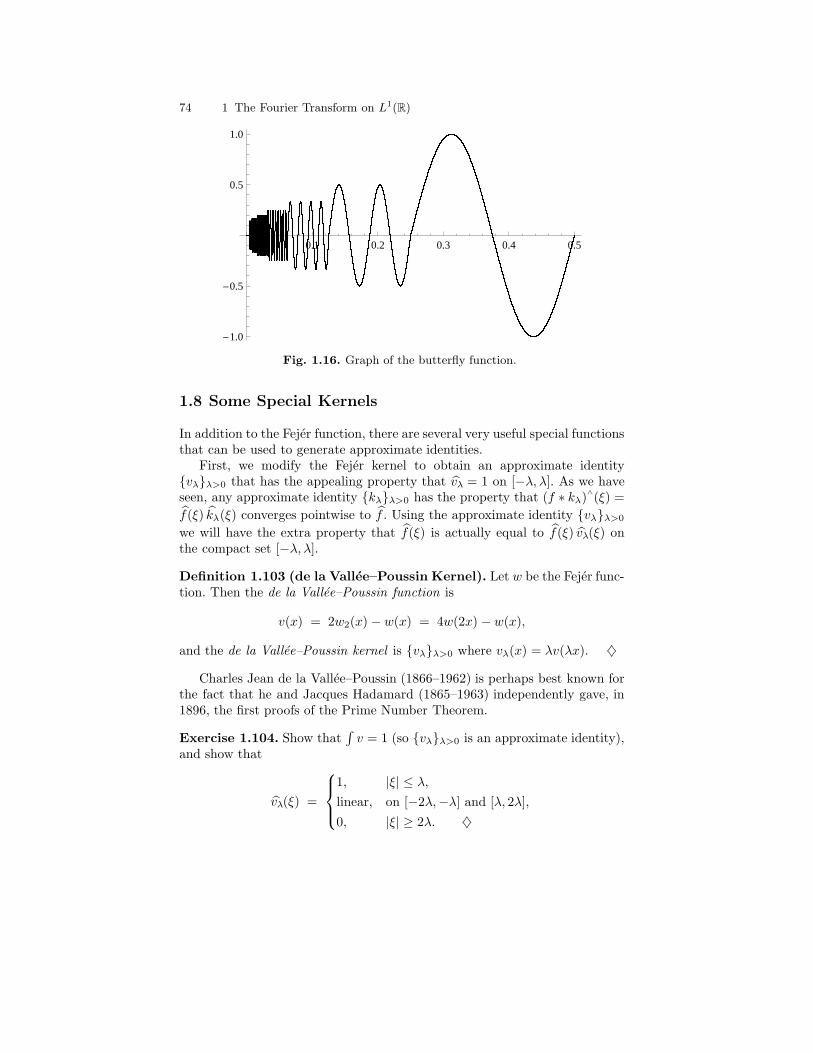
74 1 The Fourier Transform on L1(R)
0.1 0.2 0.3 0.4 0.5
-1.0
-0.5
0.5
1.0
Fig. 1.16. Graph of the butterfly function.
1.8 Some Special Kernels
In addition to the Fejer function, there are several very useful special functionsthat can be used to generate approximate identities.
First, we modify the Fejer kernel to obtain an approximate identityvλλ>0 that has the appealing property that vλ = 1 on [−λ, λ]. As we haveseen, any approximate identity kλλ>0 has the property that (f ∗ kλ)
∧
(ξ) =
f(ξ) kλ(ξ) converges pointwise to f . Using the approximate identity vλλ>0
we will have the extra property that f(ξ) is actually equal to f(ξ) vλ(ξ) onthe compact set [−λ, λ].
Definition 1.103 (de la Vallee–Poussin Kernel). Let w be the Fejer func-tion. Then the de la Vallee–Poussin function is
v(x) = 2w2(x) − w(x) = 4w(2x) − w(x),
and the de la Vallee–Poussin kernel is vλλ>0 where vλ(x) = λv(λx). ♦
Charles Jean de la Vallee–Poussin (1866–1962) is perhaps best known forthe fact that he and Jacques Hadamard (1865–1963) independently gave, in1896, the first proofs of the Prime Number Theorem.
Exercise 1.104. Show that∫
v = 1 (so vλλ>0 is an approximate identity),and show that
vλ(ξ) =
1, |ξ| ≤ λ,
linear, on [−2λ,−λ] and [λ, 2λ],
0, |ξ| ≥ 2λ. ♦
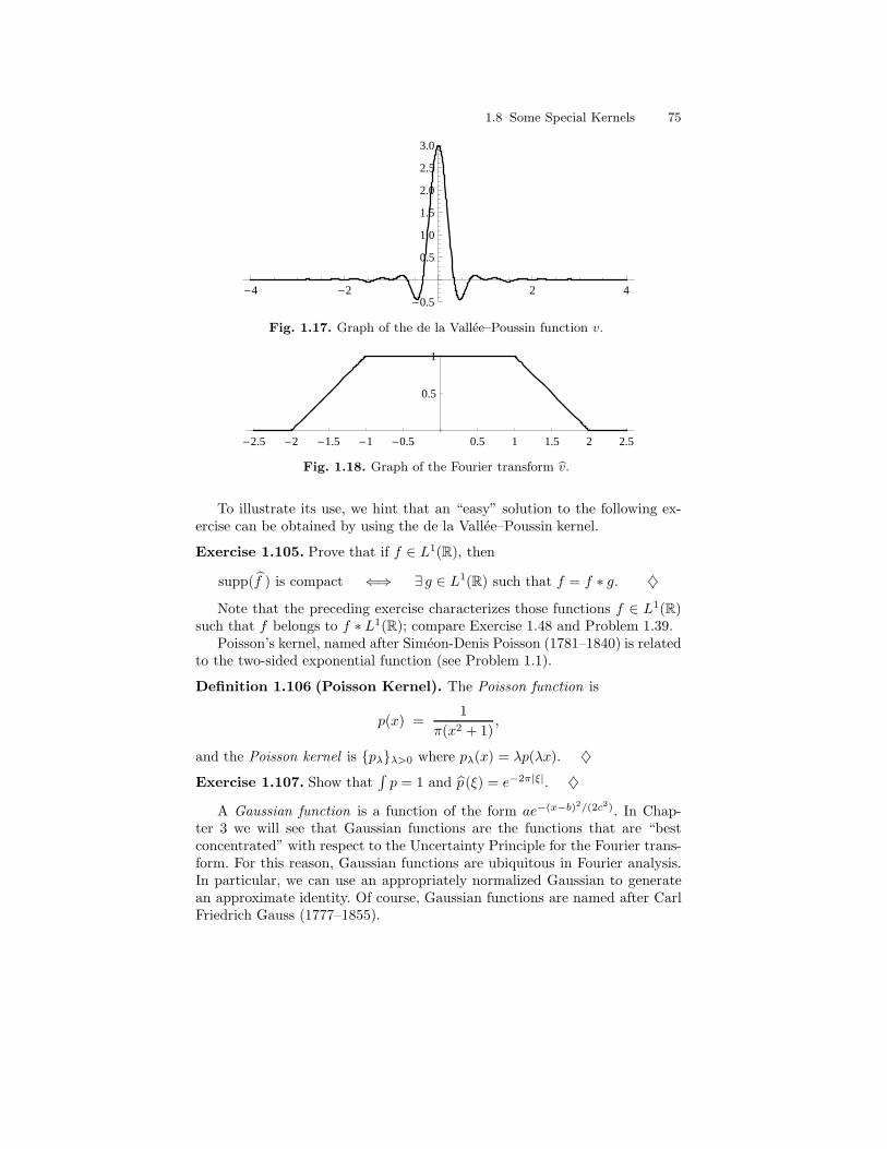
1.8 Some Special Kernels 75
-4 -2 2 4-0.5
0.5
1.0
1.5
2.0
2.5
3.0
Fig. 1.17. Graph of the de la Vallee–Poussin function v.
-2.5 -2 -1.5 -1 -0.5 0.5 1 1.5 2 2.5
0.5
1
Fig. 1.18. Graph of the Fourier transform bv.
To illustrate its use, we hint that an “easy” solution to the following ex-ercise can be obtained by using the de la Vallee–Poussin kernel.
Exercise 1.105. Prove that if f ∈ L1(R), then
supp(f ) is compact ⇐⇒ ∃ g ∈ L1(R) such that f = f ∗ g. ♦
Note that the preceding exercise characterizes those functions f ∈ L1(R)such that f belongs to f ∗ L1(R); compare Exercise 1.48 and Problem 1.39.
Poisson’s kernel, named after Simeon-Denis Poisson (1781–1840) is relatedto the two-sided exponential function (see Problem 1.1).
Definition 1.106 (Poisson Kernel). The Poisson function is
p(x) =1
π(x2 + 1),
and the Poisson kernel is pλλ>0 where pλ(x) = λp(λx). ♦Exercise 1.107. Show that
∫p = 1 and p(ξ) = e−2π|ξ|. ♦
A Gaussian function is a function of the form ae−(x−b)2/(2c2). In Chap-ter 3 we will see that Gaussian functions are the functions that are “bestconcentrated” with respect to the Uncertainty Principle for the Fourier trans-form. For this reason, Gaussian functions are ubiquitous in Fourier analysis.In particular, we can use an appropriately normalized Gaussian to generatean approximate identity. Of course, Gaussian functions are named after CarlFriedrich Gauss (1777–1855).
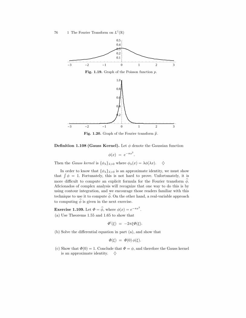
76 1 The Fourier Transform on L1(R)
-3 -2 -1 0 1 2 3
0.10.20.30.40.5
Fig. 1.19. Graph of the Poisson function p.
-3 -2 -1 0 1 2 3
0.2
0.4
0.6
0.8
1.0
Fig. 1.20. Graph of the Fourier transform bp.
Definition 1.108 (Gauss Kernel). Let φ denote the Gaussian function
φ(x) = e−πx2
.
Then the Gauss kernel is φλλ>0 where φλ(x) = λφ(λx). ♦
In order to know that φλλ>0 is an approximate identity, we must showthat
∫φ = 1. Fortunately, this is not hard to prove. Unfortunately, it is
more difficult to compute an explicit formula for the Fourier transform φ.Aficionados of complex analysis will recognize that one way to do this is byusing contour integration, and we encourage those readers familiar with this
technique to use it to compute φ. On the other hand, a real-variable approach
to computing φ is given in the next exercise.
Exercise 1.109. Let Φ = φ, where φ(x) = e−πx2
.
(a) Use Theorems 1.55 and 1.65 to show that
Φ′(ξ) = −2πξΦ(ξ).
(b) Solve the differential equation in part (a), and show that
Φ(ξ) = Φ(0)φ(ξ).
(c) Show that Φ(0) = 1. Conclude that Φ = φ, and therefore the Gauss kernelis an approximate identity. ♦
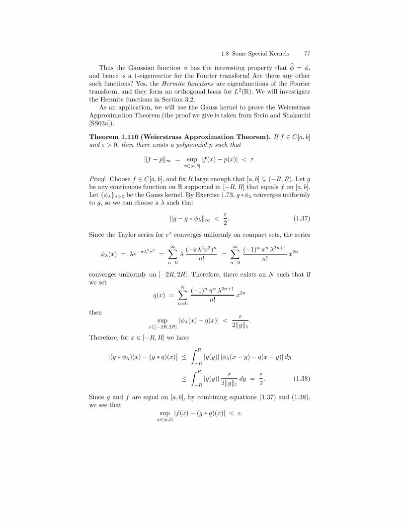
1.8 Some Special Kernels 77
Thus the Gaussian function φ has the interesting property that φ = φ,and hence is a 1-eigenvector for the Fourier transform! Are there any othersuch functions? Yes, the Hermite functions are eigenfunctions of the Fouriertransform, and they form an orthogonal basis for L2(R). We will investigatethe Hermite functions in Section 3.2.
As an application, we will use the Gauss kernel to prove the WeierstrassApproximation Theorem (the proof we give is taken from Stein and Shakarchi[SS03a]).
Theorem 1.110 (Weierstrass Approximation Theorem). If f ∈ C[a, b]and ε > 0, then there exists a polynomial p such that
‖f − p‖∞ = supx∈[a,b]
|f(x) − p(x)| < ε.
Proof. Choose f ∈ C[a, b], and fix R large enough that [a, b] ⊆ (−R, R). Let gbe any continuous function on R supported in [−R, R] that equals f on [a, b].Let φλλ>0 be the Gauss kernel. By Exercise 1.73, g∗φλ converges uniformlyto g, so we can choose a λ such that
‖g − g ∗ φλ‖∞ <ε
2. (1.37)
Since the Taylor series for ex converges uniformly on compact sets, the series
φλ(x) = λe−πλ2x2
=
∞∑
n=0
λ(−πλ2x2)n
n!=
∞∑
n=0
(−1)n πn λ2n+1
n!x2n
converges uniformly on [−2R, 2R]. Therefore, there exists an N such that ifwe set
q(x) =
N∑
n=0
(−1)n πn λ2n+1
n!x2n
thensup
x∈[−2R,2R]
|φλ(x) − q(x)| <ε
2‖g‖1.
Therefore, for x ∈ [−R, R] we have
∣∣(g ∗ φλ)(x) − (g ∗ q)(x)∣∣ ≤
∫ R
−R
|g(y)| |φλ(x − y) − q(x − y)| dy
≤∫ R
−R
|g(y)| ε
2‖g‖1dy =
ε
2. (1.38)
Since g and f are equal on [a, b], by combining equations (1.37) and (1.38),we see that
supx∈[a,b]
|f(x) − (g ∗ q)(x)| < ε.
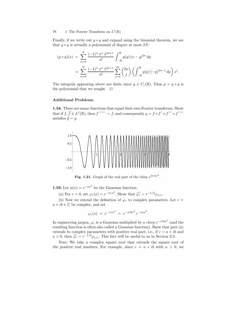
78 1 The Fourier Transform on L1(R)
Finally, if we write out g ∗ q and expand using the binomial theorem, we seethat g ∗ q is actually a polynomial of degree at most 2N :
(g ∗ q)(x) =
N∑
n=0
(−1)n πn λ2n+1
n!
∫ R
−R
g(y) (x − y)2n dy
=
N∑
n=0
(−1)n πn λ2n+1
n!
2n∑
j=0
(2n
j
) (∫ R
−R
g(y) (−y)2n−j dy
)xj .
The integrals appearing above are finite since g ∈ Cc(R). Thus p = g ∗ q isthe polynomial that we sought. ⊓⊔
Additional Problems
1.58. There are many functions that equal their own Fourier transforms. Show
that if f, f ∈ L1(R), then f∧∧∧∧
= f, and consequently g = f+f∧
+f∧∧
+f∧∧∧
satisfies g = g.
1 2 3 4
-1.0
-0.5
0.5
1.0
Fig. 1.21. Graph of the real part of the chirp e2πi2x2
.
1.59. Let φ(x) = e−πx2
be the Gaussian function.
(a) For r > 0, set ϕr(x) = e−πrx2
. Show that ϕr = r−1/2ϕ1/r.
(b) Now we extend the definition of ϕr to complex parameters. Let c =a + ib ∈ C be complex, and set
ϕc(x) = e−πcx2
= e−πibx2
e−πax2
.
In engineering jargon, ϕc is a Gaussian multiplied by a chirp e−πibx2
(and theresulting function is often also called a Gaussian function). Show that part (a)extends to complex parameters with positive real part, i.e., if c = a + ib anda > 0, then ϕc = c−1/2ϕ1/c. This fact will be useful to us in Section 3.3.
Note: We take a complex square root that extends the square root ofthe positive real numbers. For example, since c = a + ib with a > 0, we
1.9 The Schwartz Space 79
can write c = reiθ with −π/2 < θ < π/2. We take c1/2 = r1/2eiθ/2 andc−1/2 = r−1/2e−iθ/2.
Remark: If we regard e2πiξx as a “pure tone” of constant frequency, thenwe can think of e2πiξx2
as a function whose frequency increases with time, seethe illustration in Figure 1.21. If played through a speaker, such a functionsounds something like a bird’s chirp.
1.60. Suppose that f ∈ L1(R)∩L∞(R) has a jump discontinuity at the origin,i.e.,
f(0+) = limt→0+
f(t), f(0−) = limt→0−
f(t)
both exist, but f(0−) 6= f(0+). Let φλλ>0 be the Gauss kernel. Prove that
limλ→∞
(f ∗ φλ)(0) =f(0+) + f(0−)
2.
Can other kernels be used to obtain the same result?
1.61. Let f ∈ L1(R) be given. Show that if there exist δ, R > 0 such that f
is bounded on [−δ, δ] and f(ξ) ≥ 0 for |ξ| > R, then f ∈ L1(R).
1.62. Suppose that f ∈ L1(R)∩L∞(R) is real and even (so f is real and even
as well). Show that if f is not continuous, then f must change sign infinitelyoften. Thus, a “local” (jump) discontinuity of f forces a global “reaction”
in f .On the other hand, show that g(x) = ie−|x|
(χ[0,∞)−χ(−∞,0)
)has a single
jump discontinuity and that g is real and changes sign only once. Still, thefact that g has a discontinuity implies that g decays slowly.
1.63. Prove the following version of Bernstein’s Inequality. Suppose that f ∈L1(R) is differentiable and supp(f ) ⊆ [−R, R]. Show that ‖f ′‖p ≤ CR ‖f‖p
for each 1 ≤ p ≤ ∞, where C is a fixed constant independent of f, R, or p.
1.9 The Schwartz Space
The Schwartz space will play an important role throughout the rest of thisvolume. In this section, after giving its definition and basic properties, we willdiscuss its special place in harmonic analysis.
The Schwartz space is a space of infinitely differentiable functions that,together with all their derivatives, “decay rapidly” at infinity. It is namedin honor of Laurent Schwartz (1915–2002), because of its role in the theoryof distributions, which he developed. Distributions will be the focus of ourattention in Chapter 4.
80 1 The Fourier Transform on L1(R)
1.9.1 Definition and Basic Properties
The precise definition of the Schwartz space is as follows.
Definition 1.111 (The Schwartz Space). The Schwartz space is
S(R) =f ∈ C∞(R) : xmf (n)(x) ∈ L∞(R) for all m, n ≥ 0
.
An element of S(R) is called a Schwartz-class function. ♦
Thus, “rapid decay” means decay faster than the reciprocal of any poly-nomial: For each m, n ≥ 0 there exists a constant Cmn such that
|f (n)(x)| ≤ Cmn
|xm| , x ∈ R.
The constants Cmn need not be uniformly bounded in m and n.A consequence of rapid decay is that f and every derivative of f is inte-
grable.
Exercise 1.112. Show that if f ∈ S(R) then for every m, n ≥ 0 we havexmf (n)(x) ∈ L1(R) ∩ C0(R), with
‖xmf (n)(x)‖1 ≤ 2 ‖xmf (n)(x)‖∞ + 2 ‖xm+2f (n)(x)‖∞. ♦
Since C∞c (R) ⊆ S(R), we know that S(R) is dense in Lp(R) for every
1 ≤ p < ∞, and also is dense in C0(R) in L∞-norm. The Gaussian function
e−x2
is an example of a function in S(R) that is not compactly supported.On the other hand, while the two-sided exponential e−|x| has rapid decay, itis not a Schwartz-class function since it is not differentiable at the origin.
1.9.2 Topology and Convergence in the Schwartz Space
The Schwartz space is a topological vector space but not a normed vectorspace. Instead of being determined by a single norm, the topology on S(R) isdetermined by the infinite collection of seminorms
ρmn(f) = ‖xmf (n)(x)‖∞, m, n ≥ 0.
The Schwartz space and related spaces determined by families of seminormswill be discussed in more detail in Section 4.2. For us, the meaning of con-vergence in S(R) is more important than the associated topology, and con-vergence simply means simultaneous convergence with respect to each of theseminorms ρmn.
Definition 1.113 (Convergence in S(R)). Given fk, f ∈ S(R), we say thatfk converges to f in S(R) if

1.9 The Schwartz Space 81
∀m, n ≥ 0, limk→∞
ρmn(f − fk) = 0,
Writing out the seminorms explicitly, convergence in S(R) means that
∀m, n ≥ 0, limk→∞
‖xmf (n)(x) − xmf(n)k (x)‖∞ = 0.
We write fk → f in S(R) to denote that fk converges to f in S(R). ♦Because S(R) is determined by only countably many seminorms, it is pos-
sible to create a metric on S(R) that determines the convergence criterion. Inparticular, if we define
d(f, g) =∑
m,n≥0
1
2m+n
ρmn(f − g)
1 + ρmn(f − g),
then fk → f in S(R) if and only if d(f, fk) → 0 (see Exercise 4.12). Unfortu-nately, there is no norm that induces this metric on S(R), but the fact thatthere is an underlying metric means that we can define convergence in termsof ordinary sequences indexed by the natural numbers instead of having touse abstract nets, as is required in generic topological spaces (see [Heil11b,Chap. 1] for details).
Since we have a metric, we can ask whether S(R) is complete with respectto this metric. The answer is yes, every Cauchy sequence in S(R) convergesin S(R) (see Exercise 4.14). Thus S(R) is a vector space whose topology isgenerated by a metric, and it is complete with respect to that metric. Such aspace is called a Frechet space.
Since we have defined convergence in S(R), we also have a notion of conti-nuity. For example, a functional µ : S(R) → C is continuous if fk → f in S(R)implies that 〈fk, µ〉 → 〈f, µ〉, where 〈f, µ〉 denotes the action of the functionalµ on the vector f. The space of all continuous linear functionals on S(R), i.e.,the dual space of S(R), is the space of tempered distributions, denoted S ′(R).It will be a major center of attention in Chapter 4.
1.9.3 Invariance of the Schwartz Space
Now that we have introduced the Schwartz space, let us explain why it isso interesting to us. The definition of the Schwartz space incorporates bothsmoothness and decay—an element f of S(R) is both infinitely smooth anddecays rapidly at infinity (as do all of its derivatives). The Fourier transforminterchanges smoothness and decay. Thus, since f ∈ S(R) has both smooth-
ness and decay, f has both decay and smoothness, suggesting that we mayhave f ∈ S(R). And in fact this is true: The Schwartz space is invariant underthe Fourier transform. In order to prove this, we first need the reader to verifythat an application of Theorems 1.55 and 1.65 implies the following relationbetween derivatives and products. To simplify notation, we let D denote thedifferentiation operator:
Df(x) = f ′(x). (1.39)
82 1 The Fourier Transform on L1(R)
Exercise 1.114. Show that if xjf (k)(x) ∈ L1(R) for j = 0, . . . , m and k =0, . . . , n, then
(Dn
((−2πix)mf(x)
))∧
(ξ) = (2πiξ)n Dmf(ξ). ♦
Theorem 1.115 (Invariance of the Schwartz Space). The Fourier trans-form is a bijection of S(R) onto itself.
Proof. Suppose that f ∈ S(R). Then, by the product rule, we have for anym, n ≥ 0 that
Dn((−2πix)mf(x)
)=
n∑
j=0
(n
j
)Dj(−2πix)m f (n−j)(x) ∈ L1(R).
Hence,
(2πiξ)n Dmf(ξ) =(Dn
((−2πix)mf(x)
))∧
(ξ) ∈ L∞(R).
Since this is true for every m and n, we conclude that f ∈ S(R). Thus theFourier transform maps S(R) into itself, and we know that it is injective bythe Uniqueness Theorem.
On the other hand, we also have∨
f ∈ S(R), and therefore (∨
f )∧ ∈ S(R).
Hence f = (∨
f )∧
by the Inversion Formula, so the Fourier transform is surjec-tive. ⊓⊔
Not only is the Fourier transform a bijection, but it is a topological iso-morphism (or homeomorphism) of S(R) onto itself, i.e., both F and F−1 arecontinuous with respect to the topology of the Schwartz space.
Exercise 1.116 (Continuity of the Fourier Transform on S(R)). Givenany m, n ≥ 0, show that there exist constants Cjℓ > 0 such that
‖ξnf (m)(ξ)‖∞ ≤m∑
j=0
n∑
ℓ=0
Cjℓ ‖xjf (ℓ)(x)‖1.
Use this to show that F : S(R) → S(R) is continuous, i.e.,
fk → f in S(R) =⇒ fk → f in S(R),
and similarly F−1 : S(R) → S(R) is continuous. ♦
As a final remark, we note that since C∞c (R) ⊆ S(R), the Fourier transform
maps C∞c (R) into S(R):
f ∈ C∞c (R) =⇒ f ∈ S(R).

1.9 The Schwartz Space 83
However, we will later see the Paley–Wiener Theorem (Theorem 3.49), which
implies that f and f cannot both be compactly supported (unless f = 0).Hence the Fourier transform does not map C∞
c (R) into itself:
F(C∞
c (R))
⊆ S(R) but F(C∞
c (R))∩ C∞
c (R) = 0.
Similarly, if f ∈ L1(R) and f ∈ C∞c (R), then f ∈ S(R), so we know that
f ∈ S(R), but f cannot be compactly supported.
Additional Problems
1.64. Show that if f ∈ S(R) and g ∈ C∞b (R), then fg ∈ S(R). In particular,
S(R) is closed under pointwise products.
1.65. Show that if f ∈ S(R) and xmg(x) ∈ L1(R) for every m ≥ 0, thenf ∗ g ∈ S(R). In particular, S(R) is closed under convolution.
1.66. Show thatf ∈ L1(R) : f ∈ C∞
c (R)
is dense in Lp(R) for each 1 ≤p < ∞.
1.67. Construct a function f ∈ S(R) that satisfies limn→∞ |f (n)(n)| = ∞.


![[John Heil, Alfred Mele] Mental Causation](https://static.fdocuments.us/doc/165x107/55cf9a9f550346d033a29fa7/john-heil-alfred-mele-mental-causation.jpg)


![Kantharos [Elliger, Fink, Heil, Meyer]](https://static.fdocuments.us/doc/165x107/5695d2a01a28ab9b029b2606/kantharos-elliger-fink-heil-meyer.jpg)


