Genetics: Fundamentals of Mendelian Genetics Classical Genetics.

Introduction to Genetics
Bruce Walsh lecture notesUppsala EQG courseversion 28 Jan 2012

Topics• Darwin and Mendel
• Mendel genetics– Mendel's experiments
– Mendel's laws
• Genes and chromosomes– Linkage
– Prior probability of linkage
• Genes and DNA– Basics of DNA structure
– Types of Genetic markers

Darwin & Mendel• Darwin (1859) Origin of Species
– Instant Classic, major immediate impact
– Problem: Model of Inheritance• Darwin assumed Blending inheritance
• Offspring = average of both parents
• zo = (zm + zf)/2
• Fleming Jenkin (1867) pointed out problem
– Var(zo) = Var[(zm + zf)/2] = (1/2) Var(parents)
– Hence, under blending inheritance, half the variation isremoved each generation and this must somehow bereplenished by mutation.

Mendel

Mendel• Mendel (1865), Experiments in Plant Hybridization
• No impact, paper essentially ignored– Ironically, Darwin had an apparently unread copy in his
library
– Why ignored? Perhaps too mathematical for 19thcentury biologists
• The rediscovery in 1900 (by three independentgroups)
• Mendel’s key idea: Genes are discrete particlespassed on intact from parent to offspring

Mendel’s experiments with the Garden Pea
7 traits examined

Mendel crossed a pure-breeding yellow pea linewith a pure-breeding green line.
Let P1 denote the pure-breeding yellow (parental line 1)P2 the pure-breed green (parental line 2)
The F1, or first filial, generation is the cross ofP1 x P2 (yellow x green).
All resulting F1 were yellow
The F2, or second filial, generation is a cross of two F1’s
In F2, 1/4 are green, 3/4 are yellow
This outbreak of variation blows the theory of blending inheritance right out of the water.

Mendel also observed that the P1, F1 and F2 Yellow lines behaved differently when crossed to pure green
P1 yellow x P2 (pure green) --> all yellow
F1 yellow x P2 (pure green) --> 1/2 yellow, 1/2 green
F2 yellow x P2 (pure green) --> 2/3 yellow, 1/3 green
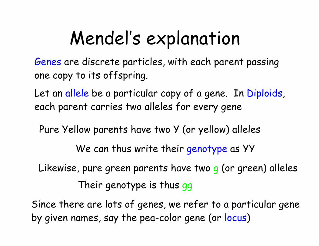
Mendel’s explanationGenes are discrete particles, with each parent passingone copy to its offspring.
Let an allele be a particular copy of a gene. In Diploids,each parent carries two alleles for every gene
Pure Yellow parents have two Y (or yellow) alleles
We can thus write their genotype as YY
Likewise, pure green parents have two g (or green) alleles
Their genotype is thus gg
Since there are lots of genes, we refer to a particular geneby given names, say the pea-color gene (or locus)
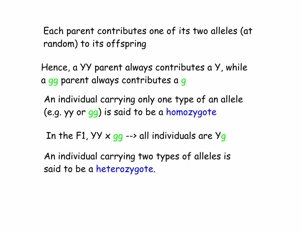
Each parent contributes one of its two alleles (atrandom) to its offspring
Hence, a YY parent always contributes a Y, whilea gg parent always contributes a g
In the F1, YY x gg --> all individuals are Yg
An individual carrying only one type of an allele(e.g. yy or gg) is said to be a homozygote
An individual carrying two types of alleles issaid to be a heterozygote.

The phenotype of an individual is the trait value weobserve
For this particular gene, the map from genotype tophenotype is as follows:
YY --> yellow
Yg --> yellow
gg --> green
Since the Yg heterozygote has the same phenotypicvalue as the YY homozygote, we say (equivalently)
Y is dominant to g, or
g is recessive to Y

Explaining the crosses
F1 x F1 -> Yg x Yg
Prob(YY) = yellow(dad)*yellow(mom) = (1/2)*(1/2)
Prob(gg) = green(dad)*green(mom) = (1/2)*(1/2)
Prob(Yg) = 1-Pr(YY) - Pr(gg) = 1/2
Prob(Yg) = yellow(dad)*green(mom) + green(dad)*yellow(mom)
Hence, Prob(Yellow phenotype) = Pr(YY) + Pr(Yg) = 3/4
Prob(green phenotype) = Pr(gg) = 1/4

Review of terms (so far)
• Gene
• Locus
• Allele
• Homozygote
• Heterozygote
• Dominant
• Recessive
• Genotype
• Phenotype

In class problem (5 minutes)Explain why F2 yellow x P2 (pure green) - -> 2/3 yellow, 1/3 green
F2 yellows are a mix, being either Yg or YY
Prob(F2 yellow is Yg) = Pr(yellow | Yg)*Pr(Yg in F2)
Pr(Yellow)
= (1* 1/2)/(3/4) = 2/3
2/3 of crosses are Yg x gg -> 1/2 Yg (yellow), 1/2 gg (green)
1/3 of crosses are YY x gg -> all Yg (yellow)
Pr(yellow) = (2/3)*(1/2) + (1/3) = 2/3

Dealing with two (or more) genes
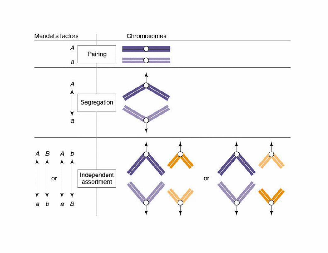
For his 7 traits, Mendel observed Independent Assortment
The genotype at one locus is independent of the second
RR, Rr - round seeds, rr - wrinkled seeds
Pure round, green (RRgg) x pure wrinkled yellow (rrYY)
F1 --> RrYg = round, yellow
What about the F2?

Let R- denote RR and Rr. R- are round. Note in F2,Pr(R-) = 1/2 + 1/4 = 3/4
Likewise, Y- are YY or Yg, and are yellow
(1/4)*(1/4) = 1/16ggrrGreen, wrinkled
(1/4)*(3/4) = 3/16ggR-Green, round
(3/4)*(1/4) = 3/16Y-rrYellow, wrinkled
(3/4)*(3/4) = 9/16Y-R-Yellow, round
FrequencyGenotypePhenotype
Or a 9:3:3:1 ratio

Probabilities for more complex genotypes
Cross AaBBCcDD X aaBbCcDd
What is Pr(aaBBCCDD)?
Under independent assortment, = Pr(aa)*Pr(BB)*Pr(CC)*Pr(DD) = (1/2*1)*(1*1/2)*(1/2*1/2)*(1*1/2) = 1/25
What is Pr(AaBbCc)?
= Pr(Aa)*Pr(Bb)*Pr(Cc) = (1/2)*(1/2)*(1/2) = 1/8

Mendel was wrong: Linkage
2455ppllRed round
7121ppL-Red long
7121P-llPurple round
215284P-L-Purple long
ExpectedObservedGenotypePhenotype
Bateson and Punnet looked at flower color: P (purple) dominant over p (red )
pollen shape: L (long) dominant over l (round)
Excess of PL, pl gametes over Pl, pL
Departure from independent assortment

Interlude: Chromosomal theory ofinheritance
It was soon postulated that Genes are carried on chromosomes, because chromosomes behaved in afashion that would generate Mendel’s laws.
Early light microscope work on dividing cells revealedsmall (usually) rod-shaped structures that appear topair during cell division. These are chromosomes.
We now know that each chromosome consists of asingle double-stranded DNA molecule (covered withproteins), and it is this DNA that codes for the genes.

Humans have 23 pairs of chromosomes (for a total of 46)
22 pairs of autosomes (chromosomes 1 to 22)
1 pair of sex chromosomes -- XX in females, XY in males
Humans also have another type of DNA molecule, namelythe mitochondrial DNA genome that exists in tens to thousands of copies in the mitochondria present in all ourcells
mtDNA is usual in that it is strictly maternally inherited.Offspring get only their mother’s mtDNA.

Linkage
If genes are located on different chromosomes they(with very few exceptions) show independent assortment.
Indeed, peas have only 7 chromosomes, so was Mendel luckyin choosing seven traits at random that happen to allbe on different chromosomes? Exercise: compute this probability.
However, genes on the same chromosome, especially ifthey are close to each other, tend to be passed ontotheir offspring in the same configuration as on theparental chromosomes.
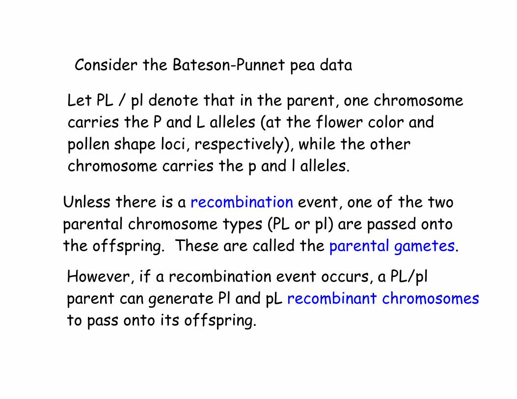
Consider the Bateson-Punnet pea data
Let PL / pl denote that in the parent, one chromosomecarries the P and L alleles (at the flower color andpollen shape loci, respectively), while the other chromosome carries the p and l alleles.
Unless there is a recombination event, one of the twoparental chromosome types (PL or pl) are passed ontothe offspring. These are called the parental gametes.
However, if a recombination event occurs, a PL/pl parent can generate Pl and pL recombinant chromosomesto pass onto its offspring.

Let c denote the recombination frequency --- theprobability that a randomly-chosen gamete from theparent is of the recombinant type (i.e., it is not aparental gamete).
For a PL/pl parent, the gamete frequencies are
1/4c/2Pl
1/4c/2pL
1/4(1-c)/2pl
1/4(1-c)/2PL
Expectation under
independent assortment
FrequencyGamete type

1/4c/2Pl
1/4c/2pL
1/4(1-c)/2pl
1/4(1-c)/2PL
Expectation under
independent assortment
FrequencyGamete type
Parental gametes in excess, as (1-c)/2 > 1/4 for c < 1/2
Recombinant gametes in deficiency, as c/2 < 1/4 for c < 1/2

Expected genotype frequencies under linkage
Suppose we cross PL/pl X PL/pl parents
What are the expected frequencies in their offspring?
Pr(PPLL) = Pr(PL|father)*Pr(PL|mother) = [(1-c)/2]*[(1-c)/2] = (1-c)2/4
Recall from previous data that freq(ppll) = 55/381 =0.144
Hence, (1-c)2/4 = 0.144, or c = 0.24
Likewise, Pr(ppll) = (1-c)2/4

A (slightly) more complicated case
Again, assume the parents are both PL/pl. Compute Pr(PpLl)
Two situations, as PpLl could be PL/pl or Pl/pL
Pr(PL/pl) = Pr(PL|dad)*Pr(pl|mom) + Pr(PL|mom)*Pr(pl|dad) = [(1-c)/2]*[(1-c)/2] + [(1-c)/2]*[(1-c)/2]
Pr(Pl/pL) = Pr(Pl|dad)*Pr(pL|mom) + Pr(Pl|mom)*Pr(pl|dad) = (c/2)*(c/2) + (c/2)*(c/2)
Thus, Pr(PpLl) = (1-c)2/2 + c2 /2

Generally, to compute the expected genotypeprobabilities, need to consider the frequenciesof gametes produced by both parents.
Suppose dad = Pl/pL, mom = PL/pl
Pr(PPLL) = Pr(PL|dad)*Pr(PL|mom) = [c/2]*[(1-c)/2]
Notation: when PL/pl, we say that alleles P and Lare in coupling
When parent is Pl/pL, we say that P and L are in repulsion

Genetic Maps and Mapping Functions
The unit of genetic distance between two markers isthe recombination frequency, c (also called !)
If the phase of a parent is AB/ab, then 1-c is thefrequency of “parental” gametes (e.g., AB and ab),while c is the frequency of “nonparental” gametes(e.g.. Ab and aB).
A parental gamete results from an EVEN number ofcrossovers, e.g., 0, 2, 4, etc.
For a nonparental (also called a recombinant) gamete,need an ODD number of crossovers between A & be.g., 1, 3, 5, etc.
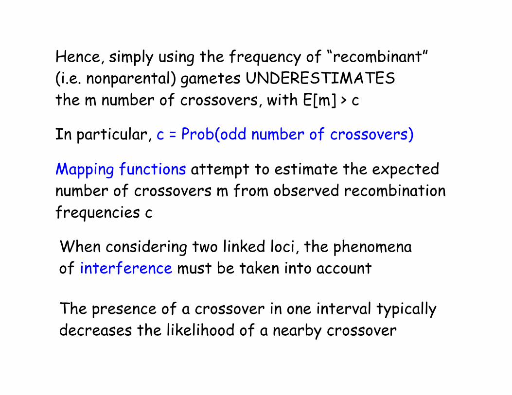
Hence, simply using the frequency of “recombinant”(i.e. nonparental) gametes UNDERESTIMATESthe m number of crossovers, with E[m] > c
Mapping functions attempt to estimate the expectednumber of crossovers m from observed recombinationfrequencies c
When considering two linked loci, the phenomenaof interference must be taken into account
The presence of a crossover in one interval typicallydecreases the likelihood of a nearby crossover
In particular, c = Prob(odd number of crossovers)

cAC = cAB (1 − cBC) + (1 − cAB) cBC = cAB + cBC −2cAB cBC
Suppose the order of the genes is A-B-C.
If there is no interference (i.e., crossovers occurindependently of each other) then
Probability(odd number of crossovers btw A and C)
Even number of crossovers btw A & B, Odd number between B & C
odd number in A-B, even number in B-C

cAC = cAB + cBC − 2(1− δ)cAB cBC
We need to assume independence of crossovers inorder to multiply these two probabilities
When interference is present, we can write this as
Interference parameter
" = 1 --> complete interference: The presence of a crossover eliminates nearby crossovers
" = 0 --> No interference. Crossovers occur independently of each other

Mapping functions. Moving from c to m
Haldane’s mapping function (gives Haldane mapdistances)
Assume the number k of crossovers in a regionfollows a Poisson distribution with parameter m
This makes the assumption of NO INTERFERENCE
Pr(Poisson = k) = #k Exp[-#]/k! # = expected number of successes
c =∞∑
k=0
p(m, 2k + 1) = e−m∞∑
k=0
m2k+1
(2k + 1)!=
1− e−2m
2

Prob(Odd number of crossovers)
Odd number
Usually reported in units of Morgans or Centimorgans (Cm)
One morgan --> m = 1.0. One cM --> m = 0.01
c =∞∑
k=0
p(m, 2k + 1) = e−m∞∑
k=0
m2k+1
(2k + 1)!=
1− e−2m
2
m = −ln(1−2c)2
This gives the estimated Haldane distance as
Relates recombination fraction c to expected numberof crossovers m
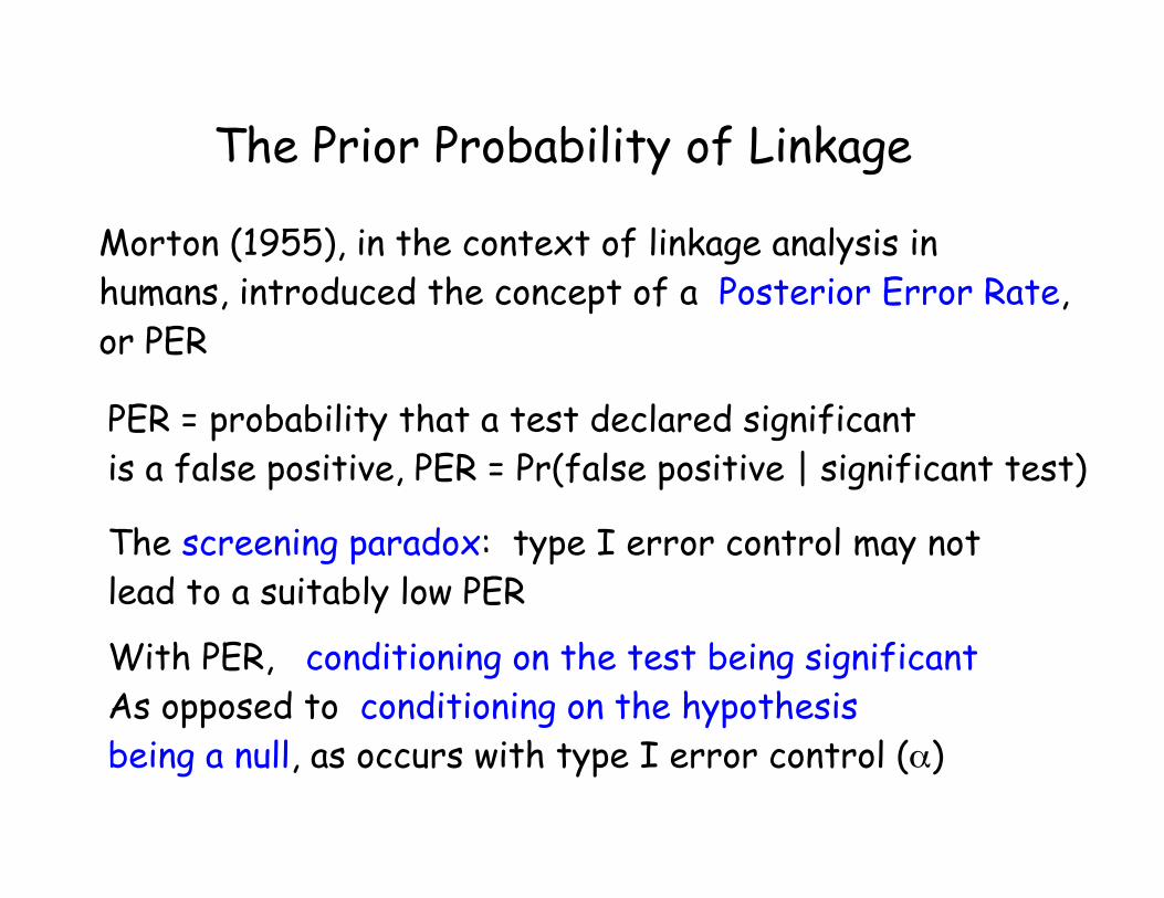
The Prior Probability of Linkage
Morton (1955), in the context of linkage analysis inhumans, introduced the concept of a Posterior Error Rate,or PER
PER = probability that a test declared significantis a false positive, PER = Pr(false positive | significant test)
The screening paradox: type I error control may notlead to a suitably low PER
With PER, conditioning on the test being significant,As opposed to !conditioning on the hypothesisbeing a null, as occurs with type I error control ($)

Let $ be the Type 1 error, % the type 2 error (1- % = power)And & be the fraction of null hypothesis, then from Bayes’ theorem
PER = Pr(false positive | significant)
Pr(false positive | null True )* Pr(null)
Pr(significant test)PER =
Since there are !23 pairs of human chromosomes, Morton argued that two randomly-chosen genes had a 1/23 (roughly 5%) prior probability of linkage, i.e. & = 0.95

This is because most of the hypotheses are expected to null.If we draw 1000 random pairs of loci, 950 !are expected to be unlinked, and we expect !950 * 0.05 = 47.5 of these to show a false-positive. Conversely, only 50 are expected to be linked, and we would declare 50 * 0.80 = 40 of these to be significant, so that 47.5/87.5 of the significant results are due to false-positives.
Assuming $ type I error of a = 0.05 and 80% power(% = 0.2), the expected PER is
0.05*0.95
0.05*0.95 + 0.8*0.05= 0.54
Hence, even with a 5% type-I error control, a randomsignificant test has a 54% chance of being a false-positive.

Molecular MarkersYou and your neighbor differ at roughly 22,000,000 nucleotides (base pairs) out of the roughly 3 billionbp that comprises the human genome
Hence, LOTS of molecular variation to exploit
SNP -- single nucleotide polymorphism. A particularposition on the DNA (say base 123,321 on chromosome 1)that has two different nucleotides (say G or A) segregating
STR -- simple tandem arrays. An STR locus consists ofa number of short repeats, with alleles defined bythe number of repeats. For example, you might have6 and 4 copies of the repeat on your two chromosome 7s

SNPs vs STRsSNPs
Cons: Less polymorphic (at most 2 alleles)
Pros: Low mutation rates, alleles very stable
Excellent for looking at historical long-termassociations (association mapping)
STRs
Cons: High mutation rate
Pros: Very highly polymorphic
Excellent for linkage studies within an extended Pedigree (QTL mapping in families or pedigrees)